EP2843184A2 - Verfahren zur Durchführung einer Stimulationsoperation mit Stützmittelplatzierung an einem Bohrplatz - Google Patents
Verfahren zur Durchführung einer Stimulationsoperation mit Stützmittelplatzierung an einem Bohrplatz Download PDFInfo
- Publication number
- EP2843184A2 EP2843184A2 EP14182269.2A EP14182269A EP2843184A2 EP 2843184 A2 EP2843184 A2 EP 2843184A2 EP 14182269 A EP14182269 A EP 14182269A EP 2843184 A2 EP2843184 A2 EP 2843184A2
- Authority
- EP
- European Patent Office
- Prior art keywords
- fracture
- proppant
- asperity
- fractures
- conductivity
- Prior art date
- Legal status (The legal status is an assumption and is not a legal conclusion. Google has not performed a legal analysis and makes no representation as to the accuracy of the status listed.)
- Withdrawn
Links
Images


Classifications
-
- E—FIXED CONSTRUCTIONS
- E21—EARTH OR ROCK DRILLING; MINING
- E21B—EARTH OR ROCK DRILLING; OBTAINING OIL, GAS, WATER, SOLUBLE OR MELTABLE MATERIALS OR A SLURRY OF MINERALS FROM WELLS
- E21B43/00—Methods or apparatus for obtaining oil, gas, water, soluble or meltable materials or a slurry of minerals from wells
- E21B43/25—Methods for stimulating production
- E21B43/26—Methods for stimulating production by forming crevices or fractures
- E21B43/267—Methods for stimulating production by forming crevices or fractures reinforcing fractures by propping
-
- G—PHYSICS
- G06—COMPUTING OR CALCULATING; COUNTING
- G06F—ELECTRIC DIGITAL DATA PROCESSING
- G06F30/00—Computer-aided design [CAD]
- G06F30/20—Design optimisation, verification or simulation
Definitions
- At least one embodiment relates to techniques for performing oilfield operations. More particularly, at least one embodiment of the present disclosure relates to techniques for performing stimulation operations, such as perforating, injecting, and/or fracturing, a subterranean formation having at least one reservoir therein.
- Hydraulic fracturing may be used to create cracks in subsurface formations to allow oil or gas to move toward the well.
- a formation is fractured by introducing a specially engineered fluid (referred to as "fracturing fluid”, “treatment fluid”, or “fracturing slurry” herein) at high pressure and high flow rates into the formation through one or more wellbores.
- Hydraulic fractures may extend away from the wellbore hundreds of feet in opposing directions according to the natural stresses within the formation. Under certain circumstances, they may form a complex fracture network.
- Complex fracture networks may include induced hydraulic fractures and natural fractures, which may or may not intersect, along multiple azimuths, in multiple planes and directions, and in multiple regions.
- Patterns of hydraulic fractures created by the fracturing stimulation may be complex and may form a fracture network as indicated by a distribution of associated microseismic events.
- Complex hydraulic fracture networks have been developed to represent the created hydraulic fractures. Examples of fracture models and fracture simulators are provided in US Patent/Application Nos. 6101447 , 7363162 , 7788074 , 8412500 , 20120179444 , 20080133186 , 20100138196 , 20100250215 , 6776235 , 8584755 , and 8066068 , the entire contents of which are hereby incorporated by reference herein.
- Fracturing fluids may be injected into the wellbore in a manner that provides the desired fractures.
- the fracturing fluids may include proppants to prop fractures open and facilitate fluid flow to the wellbore. Examples of fracturing and/or proppant techniques are provided in US Patent/Application Nos. 6776235 , 8066068 , 8490700 , 8584755 , 7581590 , and 7451812 , the entire contents of which are hereby incorporated by reference herein.
- the present disclosure relates to a method for performing a stimulation operation at a wellsite.
- the wellsite has a wellbore penetrating a formation having fractures therein.
- the method involves predicting placement of proppant in the fractures based on wellsite data (including geometry of the fractures), generating an asperity model based on the predicted placement, predicting aperture change for a prescribed closure stress using the asperity model, determining fracture conductivity based on the predicted aperture change, and placing proppant into the fractures with a stimulation fluid by injecting the stimulation fluid having the proppant therein into the formation based on the determined fracture conductivity.
- the disclosure relates to a method for performing a stimulation operation at a wellsite.
- the wellsite has a wellbore penetrating a formation having fractures therein.
- the method involves determining proppant parameters of the fractures by predicting placement of proppant in the fractures based on wellsite data using a plurality of simulations (the wellsite data comprising geometry of the fractures), generating an asperity model based on the predicted placement, predicting aperture change for a prescribed closure stress using the asperity model, determining fracture conductivity based on the predicted aperture change, and validating the predicted placement by comparing the plurality of simulations, and placing proppant into the fractures with a stimulation fluid by injecting the stimulation fluid having the proppant therein into the formation based on the validated fracture conductivity.
- the disclosure relates to a method for stimulating a wellbore at a wellsite.
- the wellsite has a wellbore penetrating a formation having fractures therein.
- the method involves determining proppant parameters of the fractures by predicting placement of proppant in the fractures based on wellsite data, the wellsite data comprising geometry of the fractures, generating an asperity model based on the predicted placement, predicting aperture change for a prescribed closure stress using the asperity model, and determining fracture conductivity based on the predicted aperture change, and placing proppant into the fractures with a stimulation fluid by injecting the stimulation fluid having the proppant therein into the formation based on the validated fracture conductivity, and producing fluid from the reservoirs and into the wellbore through the propped fractures.
- the present disclosure provides a method for performing a stimulation operation at a wellsite.
- the stimulating involves generating proppant parameters by predicting placement of proppant in fractures, generating an asperity model (sometimes referred to as an asperity-based model) based on the prediction, predicting aperture change for a given closure stress using the asperity model, and determining fracture conductivity based on the closure stress.
- the proppant may then be placed into the fractures by injecting a stimulation fluid with the proppant therein into the formation based on the determined fracture conductivity. Reservoir fluids may then be produced through the propped fractures.
- the predicting may optionally be validated by comparison with other predictions and/or measurements. Placement of proppant and the resultant conductivity within a rough fracture may be predicted under any prescribed closure stress.
- the rough fracture may be represented by a collection of asperities, which may be arranged upon a regular grid attached to two deformable half-spaces.
- the deformation characteristics of the deformable half-spaces may be pre-calculated, allowing for efficient prediction of the deformation of the formation on either side of the fracture.
- the present disclosure provides a method for automatically detecting additional contact as the fracture closes during increasing closure stress (such as during flow-back and production).
- the asperity mechanical response can be modified to account for a combined mechanical response of the rough fracture surface and proppant that may be present in the fracture at that location. In this way, the deformation of any combination of fracture roughness and heterogeneous arrangement of proppant in the fracture may be evaluated.
- Another approach approximates detailed asperities with a more coarse collection of cylinders for the mechanical calculation.
- the deformed state is then converted into a pore network model which calculates the conductivity of the fracture during flow-back and subsequent production.
- This alternative approach may be faster than the first approach and may have reduced accuracy.
- the approaches may be compared for validation and/or to detect issues, such as water injection and multiple fluid interactions.
- the methods for predicting proppant placement may involve consideration of the interplay between fracture roughness, generalized heterogeneous proppant geometry and proppant compliance. Such placement may be intended to efficiently simulate detailed, arbitrary proppant arrangements, including the natural roughness of real fractures in detail and capturing nonlinear stiffening behavior of the fracture as it closes.
- Placement may utilize accelerated solutions by pre-calculating the mechanical response of the formation on the grid of consideration. Such placement may take into account the following mechanisms: arbitrary distribution of proppant within the fracture; mechanical deformation of both the proppant and host rock; roughness of the fracture surface in detail; feedback of stress redistribution as fracture surfaces make additional contact; and flow between the deformed fracture surfaces and within the heterogeneously placed proppant within the gap between the surfaces.
- Proppant placement may be used to uniformly fill a fracture with proppant in order to maintain adequate fracture aperture. By uniformly filling fractures, reservoir fluids may then be produced back through the proppant.
- Heterogeneous Proppant Placement (HPP) strategies seek to increase propped fracture conductivity by selectively placing the proppant such that the fracture is held open at discrete locations and the reservoir fluids can be transported through open channels between the proppant.
- HPP An example of HPP technology is HiWAYTM, commercially available from SCHLUMBERGERTM, Ltd. Of Houston, TX (see: www.slb.com). Additional descriptions of proppant technology are provided, for example, in US6776235 , US8066068 , and US8584755 , previously incorporated by reference herein.
- HPP may be used to introduce proppant into the fractures in discrete slugs. Mixing of the proppant slugs with clean slugs may be limited by the presence of fibers.
- the slugs may be transported down the wellbore and into the fractures with the goal of creating isolated pillars which support the fracture against closure stress, while preserving pristine flow channels in the space between.
- tools may be developed for predicting conductivity of the heterogeneously propped fractures during the increase in closure stress resulting from flow-back and subsequent production.
- the wellsite 100 has a wellbore 104 extending from a wellhead 108 at a surface location and through a subterranean formation 102 therebelow.
- a fracture network 106 extends about the wellbore 104.
- a pump system 129 is positioned about the wellhead 108 for passing fluid through tubing 142.
- the pump system 129 is depicted as being operated by a field operator 127 for recording maintenance and operational data and/or performing the operation in accordance with a prescribed pumping schedule.
- the pumping system 129 pumps fluid from the surface to the wellbore 104 during the fracture operation.
- the pump system 129 may include a water source, such as a plurality of water tanks 131, which feed water to a gel hydration unit 133.
- the gel hydration unit 133 combines water from the tanks 131 with a gelling agent to form a gel.
- the gel is then sent to a blender 135 where it is mixed with a proppant from a proppant transport 137 to form a fracturing fluid.
- the gelling agent may be used to increase the viscosity of the fracturing fluid, and to allow the proppant to be suspended in the fracturing fluid. It may also act as a friction reducing agent to allow higher pump rates with less frictional pressure.
- the fracturing fluid is then pumped from the blender 135 to the treatment trucks 120 with plunger pumps as shown by solid lines 143.
- Each treatment truck 120 receives the fracturing fluid at a low pressure and discharges it to a common manifold 139 (sometimes called a missile trailer or missile) at a high pressure as shown by dashed lines 141.
- the missile 139 then directs the fracturing fluid from the treatment trucks 120 to the wellbore 104 as shown by solid line 115.
- One or more treatment trucks 120 may be used to supply fracturing fluid at a desired rate.
- Each treatment truck 120 may be normally operated at any rate, such as well under its maximum operating capacity. Operating the treatment trucks 120 under their operating capacity may allow for one to fail and the remaining to be run at a higher speed in order to make up for the absence of the failed pump.
- a computerized control system 149 may be employed to direct the entire pump system 129 during the fracturing operation.
- fracturing fluids such as conventional stimulation fluids with proppants, may be used to create fractures.
- Other fluids such as viscous gels, "slick water” (which may have a friction reducer (polymer) and water) may also be used to hydraulically fracture shale gas wells.
- Such "slick water” may be in the form of a thin fluid (e.g., nearly the same viscosity as water) and may be used to create more complex fractures, such as multiple micro-seismic fractures detectable by monitoring.
- the fracture network includes fractures located at various positions around the wellbore 104.
- the various fractures may be natural fractures 144 present before injection of the fluids, or hydraulic fractures 146 generated about the formation 102 during injection.
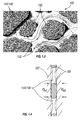
- Figure 1.2 depicts a portion 1.2 of the wellbore 104 of Figure 1.1 showing the proppant 148 placement in the formation 102.
- the proppant 148 may be pumped into the formation 102 and dispersed throughout the fracture network 106.
- the proppant 148 may be dispersed in clusters (or slugs) 150 defining channels 152 therebetween in the fractures 144/146.
- the clusters 150 may be passed into the fracture network 106 such that portions of the fractures 144/146 are propped open with the proppant 148 and portions of the fractures 144/146 remain open to transport flow to the wellbore 102 ( Figure 1.2 ) for producing fluids as schematically depicted by arrows 152 in Figure 1.3 .
- formation stresses may be applied to the proppant clusters 150 within the fractures 144/146.
- Changes in stresses ( ⁇ eff ) may affect the flow of fluid through the fractures 144/146.
- Such flow referred to as conductivity, describes the ease with which fluid move through the fractures 144/146 and may depend on permeability of the formation, saturation of the formation, and/or density and viscosity of the fluid.
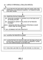
- Figure 2 is a flow chart depicting a method 200 of performing a stimulation operation.
- the method 200 may be used to determine conductivity and perform operations based on the determined conductivity.
- the method 200 involves collecting 254 wellsite data.
- the wellsite data may be from a wellsite having a wellbore penetrating a subterranean formation having fractures therein as shown in Figures 1.1-1.4 .
- the wellsite data may be, for example, wellbore sonic data, microseismic event data, wellsite equipment information, operational parameters, or other data.
- the method 200 may also involve generating 256 proppant parameters.
- the proppant parameters may be determined from the wellsite data 254.
- the predicting 256 may involve predicting 260 placement of proppant in the fractures based on the wellsite data, generating 262 an asperity model based on the proppant prediction, predicting 264 aperture change for a prescribed closure stress using the asperity model, and determining 266 fracture conductivity based on the aperture change.
- the predicting 264 and determining 266 may be repeated 268 for various closure stresses.
- the method 200 may also involve 269 validating the placement prediction, placing 270 the proppant into the fractures with a stimulation fluid, and producing 272 fluid from the formation through the fractures.
- the method may be performed at the wellsite 100 (see, e.g., Figures 1.1-1.4 ) using the equipment depicted therein. Portions of the method may be performed using, for example, the pumping system 129 to perform stimulation and the control system 149 to perform the proppant placement. Portions of the present disclosure may be performed using a processor of a computer system.
- Fracture conductivity 266 may be used to determine how to inject and/or place proppant for optimized production.
- the placing 270 may be performed by injecting the stimulation fluid having the proppant therein into the formation based on the determined fracture conductivity 266, and producing 272 fluid from the formation through the fractures.
- the method may also involve, adjusting the injecting based on new information, and other methods as desired.
- the method 200 may be performed in any order and repeated as desired.
- Figures 3-6 depict various portions of the method 200 shown in greater detail.
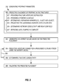
- Figure 3 depicts another view of the generating 256 proppant parameters of Figure 2 showing the predicting placement of proppant 260 in greater detail.
- the predicting 260 may involve a prediction of the placement of the proppant and other placed fluids within the rough fracture, such as the rough fracture of Figure 1.3 .
- the method of Figure 3 may also provide a detailed workflow for placement prediction within the overall fracture conductivity workflow.
- the predicting 260 may include providing 357 fracture aperture distribution and 359 a pumping schedule.
- the fracture aperture distribution 357 and pumping schedule 359 may be information provided as part of the wellsite data collected (e.g., 254 of Fig. 2 ), or may be input separately.
- the predicting 260 may also include determining the trajectory and location of 361 Lagrangian markers, projecting 363 the Lagrangian markers onto the flow grid, and determining 365 network conductivity and a flow field. The determining 361 may be based on the fracture aperture distribution 357 and the pumping schedule 359.
- the network conductivity and new flow field may be determined 365.
- the determining 361, projecting 363, and determining 365 may be repeated 367 until pumping is complete. Once complete, the remainder of the predicting 260 (e.g., 262-268) and/or method 200 (e.g., 270, 272) may be performed.
- Providing fracture aperture distribution 357 may be obtained from real or synthetic methods.
- the fracture surface geometry either measurements of real fractures can be used to dictate the surface geometry or a synthetic algorithm can be employed.
- the present disclosure utilizes a synthetic fracture generation algorithm.
- a square matrix with the same number of cells as the desired fracture is initialized with Gaussian distributed random numbers.
- a Fourier transform is performed on the matrix and this transform is then modified using a power-law, high-wave-numbers filter.
- the aperture distribution is then obtained by taking the inverse Fourier transform of the filtered spectrum.
- a digitized representation of the fracture surfaces can be obtained. Regardless of the source of data, the fracture surfaces may be approximated by a regular grid of points at which the aperture is known, bij.
- the pumping schedule may be provided 359, for example, based on the well plan for the wellsite.
- the pumping schedule may be pre-existing data provided as an input from external sources.
- the proppant parameters within the fracture may be calculated using particle placement methods, such as a Lagrangian marker of particles placed throughout the computational domain.
- the method may be performed using aspects of a Particle-in-Cell (PIC) method developed by Harlow, F.H., "A Machine Calculation Method for Hydrodynamic Problems", Los Alamos Scientific Laboratory report LAMS-1956 (1955 ), the entire contents of which are hereby incorporated by reference herein.
- PIC Particle-in-Cell
- Lagrangian markers (and/or their locations) may be determined 361 through injection and advection.
- the particles may carry information, such as the mass of gas, gel, water and proppant at that given location.
- source terms are introduced into the flow equations and Lagrangian marker particles are injected with the appropriate volume fractions of the components being injected at that time.
- the updated Lagrangian particle states may be projected 363 onto a flow grid.
- the Lagrangian particles contribute to the volume fractions of the various components within the Cartesian cell they are located within.
- the grid properties so obtained may then be used to determine local conductivities 365 using the expression for the flow of fluid between parallel plates.
- ⁇ 0 is the yield-stress of the fluid
- k is the consistency coefficient
- n is the power-law exponent
- H half the aperture of the element
- ⁇ y is the side-length of an element in the direction perpendicular to flow.
- the network conductivity and new flow field can then be determined 365 for all locations within the fracture using the approach described in Section 1.4 (Fracture Conductivity Calculation, below). If pumping is not complete the process may be repeated (367) and the new flow field can then be used to update the velocities of all Lagrangian particles within the fracture used by Equations (2) and (3) to advect the particles 361.
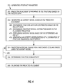
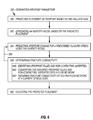
- Figure 4 depicts another portion of the predicting 256 of Figure 2 .
- the generating 262 an asperity model is shown in greater detail.
- the method of Figure 4 provides a detailed view of generation of the asperity model within the overall fracture conductivity method 256.
- the generating 262 involves developing an asperity-based representation of the combination of fracture roughness and placed proppant as obtained either from the proppant parameters 256 as described in Section 1, above or from some other independent source.
- the generating 262 involves determining 469 fracture aperture distribution, determining 471 proppant spatial distribution, performing 473 material mixing, and generating 475 an asperity representation of a combination of fracture roughness and proppant.
- System geometry such as fracture aperture distribution, may be determined 469 by the geometry of the fracture surfaces in combination with the arrangement of proppant 471 between the fracture surfaces. Mechanically, the fracture is then represented by two elastic half-spaces separated by a forest of asperities of lengths, L ij R , using the same discretization as was used in the generating 256 of Section 1.1 above.
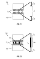
- Figure 7.1 is a schematic diagram depicting an unpropped rough natural fracture 744.
- Figure 7.2 provides a cross-section through the asperity model for the rough fracture 744 containing proppant 745. These diagrams depict a cross-section through the asperity model for the unpropped rough natural fracture 744.
- the above description along with the figures, provides a representation of the geometry and local mechanical properties of a fracture containing a heterogeneous arrangement of the proppant 475.
- Asperity lengths Lij are defined along the fracture 744.
- the present disclosure next considers the introduction of the proppant 745 into the fracture 744, filling the gaps between the rock surfaces as schematically depicted in Figure 7.2 .
- the present disclosure presumes the geometry of the proppant distribution is obtained via the predicted placement 260 and can be approximated by additional asperity lengths, L ij P , throughout the fracture.
- the present disclosure assumes that the deformation of the proppant is uniaxial (i.e.
- At least one embodiment of the present disclosure provides for approaches for predicting 264 the change in aperture due to prescribed closure stress.
- a first approach shown in Figure 5.1 , relates to "Cartesian Prediction of Aperture Change For Prescribed Closure Stress” (a Cartesian method) and uses a grid-based approach to solve the mechanical equations efficiently on the same grid as the flow using pre-calculated influence functions.
- a second approach shown in Figure 5.2 , relates to a "Cylinder-Based Prediction of Aperture Change For Prescribed Closure Stress” (a nonlinear cylinder method) which approximates the asperity grid with large cylindrical asperities for a rapid mechanical solution that is then projected back upon the original asperity grid.
- the heterogeneously propped fracture is treated as two elastic half-spaces of material, separated by asperities whose mechanical properties are obtained via generation of asperity model 262.
- asperity model 262 As described in Figure 5.1 , a method for Cartesian prediction of aperture change for a prescribed closure stress within the overall fracture conductivity workflow is provided.
- the predicting 264 involves predetermining 581 asperity-to-asperity influence (interaction) tables, adjusting 583 far-field displacement, 585 generating asperity and half-space deformation interaction based on the asperity-to-asperity influence tables, adding 587 new contacts, determining 589 if fracture is within tolerance of a target stress, and determining 591 aperture distribution from the determined asperity and half-space deformation.
- a decision may be made whether to add or delete new contacts 587. If so, the generating 585 may be repeated with the addition of new contacts. If not, the generating 264 may continue to the determining 589 and 591. The adjusting 583 may be repeated after the determining 589 and the generating 585 may be repeated when contacts are added 587.
- the predetermining of asperity-to-asperity tables 581 can be achieved by recognizing that, given an asperity, I, in contact with the half-spaces it is possible to calculate the radial dependence of the deflection of the half-space due to the asperity loading analytically or numerically.
- the analytic function or numerical result may be pre-calculated on a grid 581 upon initialization.
- the present disclosure assumes a function, ⁇ ( x',y' ), which gives the increase in aperture per unit load between the half-spaces at displacement x', y' relative to a loaded asperity.
- the present disclosure pre-determines (or pre-calculates) 581 the ⁇ IJ of equation (12) once upon initialization of the aperture change stage.
- the present disclosure obtains the stress distribution within asperities and the associated deformation of surrounding material by enforcing compatibility between the asperity stresses and associated deformation. Specifically, at any location where an asperity is in contact, the change in asperity length and the additional half-space opening at that location should be consistent.
- the far-field displacement D can be adjusted 583 to approach a requested stress state in the generation of asperity and half-space deformation interaction 585.
- the solution of this system provides the deformed state of the fracture 585. Once this deformed state is obtained, the present disclosure checks for new contact between the two surfaces due to the deformation and selects new candidate asperities for contact 587. The deformed state is then recalculated and the process is repeated until all additional points of contact have been identified.
- Figure 5.2 provides a detailed view of the predicting 264 for a cylinder-based prediction of aperture change for a prescribed closure stress within the generating 256.
- the predicting 264 involves approximating 580 an asperity grid with coarse cylinders, determining 582 for cylinder and half-space deformation consistent with applied stress, adding 584 pinch-points, and projecting 587 aperture change due to cylinders back onto the asperity grid. After the solving 582, a decision may be made whether to add or delete new pinch-points 584. If so, the solving 582 may be repeated. If not, the projecting 587 may be performed.
- Figures 8.1-8.3 are schematic views depicting proppant placement in three stages (I), (II), and (III), respectively. These figures depict conversion of (I) detailed asperity model ( Figure 8.1 - two circles and an ellipse) into (II) coarse cylinder representation ( Figure 8.2 ), and then projection back to (III) deformed detailed asperity model as part of the cylinder-based fracture deformation workflow ( Figure 8.3 ).
- Figure 8.1 shows an example of a simple prescribed, asperity-based Cartesian grid of proppant 848 distributed within a fracture 844. With the cylinder-based approach, this grid is approximated by a collection of cylinders that are much larger than the individual asperities.
- Figure 8.2 shows the coarse, cylinder-based approximation to this distribution with the proppant 848' grouped into clusters 850. The deformation and interaction among the coarse cylinders can then be calculated 582 using analytic expressions, such as the far-field approximations to the deformation of a half-space.
- the change in aperture, w IJ 2 ⁇ 1 - ⁇ 2 ⁇ Er IJ ⁇ f J
- E and ⁇ are the Young's modulus and Poisson ratio of the half-spaces
- r IJ is the distance between the two asperities.
- the determining of cylinder and half-space deformation consistent with applied stress 582 can be achieved by assembling a system of linear equations for displacement compatibility.
- the number of equations may be reduced by an order of magnitude or more compared with the Cartesian-based mechanical solution to increase efficiency.
- the coarse approximation may introduce artificial blockages or channels into the domain.
- the open channel across the top of the domain was closed by the coarse cylinder approximation.
- the change in aperture 587 may be projected back upon the original asperity grid (see Figure 8.3 ).
- Figure 8.3 shows the change in aperture for a stressed proppant pillar 848" within the fracture 844.
- artifacts such as blocked channels or new openings introduced by the coarse cylinder approximation, may be prevented from propagating back to the grid used for the conductivity calculation, and the change in aperture due to stress may be included.
- Figure 6 provides a detailed method for determining 266 fracture conductivity calculation within the generating 256.
- the determining 266 fracture conductivity involves identifying 688 proppant filled and non-contacting asperities, converting 690 the identified proppant filled and non-contacting asperities into a flow network, and obtaining 692 fracture conductivity by solving flow network at a current stress level.
- the converting 690 may involve converting cells into a flow network.
- the converting 690 may vary depending upon the state of each cell.
- the method for determining c IJ depends on whether or not the cell is proppant-filled.
- the converting of cells into a flow network 690 in the proppant-free regions of the fracture may be calculated using a network model. See, e.g., Yang. G., Cook, N.H.W., Myer, L.R., Network Modeling Of Flow In Natural Fractures, Rock Mechanics as a Guide for Efficient Utilization of Natural Resources, p. 57-64 (1989 ), the entire contents of which is hereby incorporated by reference herein.
- the fracture may be represented locally by conductive pipes where the conductivity of the pipes is calculated using the solution for flow between two parallel plates.
- the present disclosure If conductivity of the fracture at an additional closure stress is sought, the present disclosure now returns to 264 prediction of aperture change for prescribed closure stress as shown in Figure 6 . In this manner, the present disclosure obtains the conductivity of a natural, rough fracture under stress in the presence of arbitrary distributions of proppant.
- This example provides an application involving a range of fractures and proppant geometries in accordance with at least one embodiment of the present disclosure.
- the rockmass was assumed to have a Young's modulus of 20 GPa and Poisson ratio of 0.22.
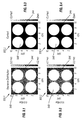
- Figures 9.1-9.4 shows results predicted by the present disclosure when applied to a fracture measuring 10 m square, with an aperture of 5 mm, containing circular proppant pillars of radius 2 m. These figures depict aperture distribution and contact distribution for the case of circular pillars of heterogeneous proppant between flat rock surfaces as predicted by the present disclosure at 0 MPa and 10 MPa closure stress.
- Figures 9.1-9.4 are graphs 900.1-900.4 depicting distributions 948,948' along an x-axis (m) and a y-axis (m) in a fracture 944 between two flat rock surfaces.
- Figures 9.1 and 9.2 shows aperture distribution 948 at 0.0 MPa and 10.0 MPa, respectively.
- Figures 9.3 and 9.4 shows contact distribution 948' at 0.0 MPa and 10.0 MPa, respectively.
- This heterogeneously propped fracture was loaded up to a closure stress of 10 MPa and fracture stiffness and fracture conductivity were calculated via application of the present disclosure. This process was then repeated for a series of fractures with different aperture geometries and proppant distributions.
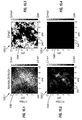
- Figures 10.1-10.4 depict aperture distribution and contact for a rough, natural fracture 944, as predicted by the present disclosure at 0 MPa and 10 MPa closure stress.
- Figures 10.1-10.4 are graphs 1000.1-1000.4 depicting distributions 1048,1048' along an x-axis (m) and a y-axis (m) in a fracture 944.
- Figures 10.1 and 10.2 shows aperture distribution 1048 at 0.0 MPa and 10.0 MPa, respectively.
- Figures 10.3 and 10.4 shows contact distribution 1048' at 0.0 MPa and 10.0 MPa, respectively.
- Figures 11.1-11.4 show the fracture 944 propped with a complicated, heterogeneous arrangement ofproppant.
- Figures 11.1-11.4 depict aperture distribution 1148 and contact distribution 1148' for an arbitrary, heterogeneous distribution within a rough, natural fracture 944 as predicted by the present disclosure for 0 MPa and 10 MPa closure stress.
- Figures 11.1-11.4 are graphs 1100.1-1100.4 depicting distributions 1148,1148' along an x-axis (m) and a y-axis (m) in a fracture 944.
- Figures 11.1 and 11.2 shows aperture distribution 1148 at 0.0 MPa and 10.0 MPa, respectively.
- Figures 11.3 and 11.4 shows contact distribution 1148' at 0.0 MPa and 10.0 MPa, respectively.
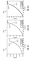
- Figures 12.1 and 12.2 are graphs 1200.1, 1200.2 showing stress versus displacement and conductivity versus stress responses, respectively, predicted for each fracture by the present disclosure.
- Figure 12.1 provides a comparison of a relationship between normal closure ( ⁇ n ) and closure stress ( ⁇ n ) for the range of proppant-fracture geometries considered.
- Graph 1200.1 depicts normal closure ( ⁇ n ) (m) (x-axis) and closure stress ( ⁇ n ) (Pa) (y-axis) for various fracture dimensions, including circular (1294.2), uniformly filled (1294.1), unpropped natural (1294.4), and heterogeneous natural (1294.3), respectively.
- Figure 12.2 provides a comparison of the evolution of fracture conductivity under closure stress for the combinations of proppant and fracture geometry considered.
- Graph 1200.2 depicts conductivity (FC) (Darcy-m)) (y-axis) and stress response ( ⁇ n ) (Pa) (x-axis) for various fracture dimensions, including circular (1294.1'), uniformly filled (1294.2'), unpropped natural (1294.3'), and heterogeneous natural (1294.4'), respectively.
- the unpropped fracture of this example exhibits the greatest closure under 10 MPa of closure stress.
- the uniformly packed smooth fracture shows the least closure with the heterogeneously packed fractures exhibiting an intermediate response.
- the conductivity of the unpropped rough fracture decreases rapidly with increasing closure stress.
- the heterogeneously propped fractures (both smooth and rough-walled) exhibit high conductivity over a wide range of closure stresses.
- Figures 13-19.3 describe additional methods relating to the predicting 256 of placement of proppant in the fractures, and for 269 validating (or verifying) the predicting 256. These methods are performed for proppant placement and pumped fluids within a rough fracture, such as those schematically depicted in Figures 7.1 and 7.2 .
- the methods may be used as part of the 260 predicting placement of proppant as described, for example, with respect to Figure 3 .
- the methods may involve analytical, 1-D, 2-D and/or 3-D simulations. Comparisons of the various methods may be used for validating 269.
- Analytical solutions such as the Herschel Bulkley solution for the flow of fluid between infinite plates, may be used as a basis for analysis of fluid flow between plates.
- the Herschel-Bulkley fluid is a generalized model of a non-Newtonian fluid, in which the strain experienced by the fluid is related to the stress in a complicated, nonlinear way. It may be assumed that the flow is fully developed locally. "Fully-developed flow” means a flow which has had sufficient distance to develop such that the local fluid velocity distribution across the aperture of the fracture depends upon the local flux, and excludes details of an upstream velocity field.
- a derivation of the Herschel-Bulkley solution may be extended using analytical solutions for power-law and Bingham fluids.
- Figure 13 depicts balance of pressure and viscous shear stress upon a rectangular region within laminar flow between parallel plates.
- ⁇ x is the length of the rectangle along axis X
- ⁇ y is the length of the rectangle along axis Y
- z is 1 ⁇ 2 the width along axis Z
- ⁇ is fluid density
- p pressure
- ⁇ zx is the shear stress.
- v x velocity
- Equation (37) may be rewritten as follows:
- Q x HB - 2 ⁇ ⁇ y ⁇ n n + 1 ⁇ P x ⁇ H - ⁇ 0 n + 1 n k 1 / n ⁇ P x 2 ⁇ 0 + n + 1 2 ⁇ n + 1 ⁇ P x ⁇ H - ⁇ 0
- Q x HB - 2 ⁇ ⁇ y ⁇ n n + 1 ⁇ P x ⁇ h / 2 - ⁇ 0 n + 1 n k 1 / n ⁇ P x 2 ⁇ 0 + n + 1 2 ⁇ n + 1 ⁇ P x ⁇ h - ⁇ 0
- This result corresponds to the case of P x > 0.
- Equation (39) may be generalized to consider an arbitrary sign of P x as follows:
- Q x HB - sgn P x ⁇ 2 ⁇ ⁇ y ⁇ n n + 1 ⁇ P x ⁇ H - ⁇ 0 n + 1 n k 1 n ⁇ P x 2 * ⁇ 0 + n + 1 2 ⁇ n + 1 ⁇ P x ⁇ H - ⁇ 0 for P x ⁇ H - ⁇ 0 > 0
- Equation (40) recovers the various sub-classes of fluid rheology in appropriate limits, such as Newtonian, power-law, and Bingham limiting cases.
- Equation (40) the solution for a Power-Law fluid limiting case is provided as follows:
- the flow of multiple non-Newtonian fluids within a variable aperture fracture may be simulated. This includes a Lagrangian particle-based approach for tracking the different phases within the fracture.
- the resultant simulation may be verified through comparison with other simulations for multiphase flow in fractures of different geometries. Agreement for a wide range of injected fluids with viscosity contrasts spanning many orders of magnitude may be obtained.
- Equation (40) a relationship between pressure drop and flux that, combined with local flux conservation, leads to a set of nonlinear simultaneous equations for the unknown p i .
- Equation (40) The solution may be obtained by iteratively solving a linearized form of Equation (40). Note that in the limit of small ⁇ 0 and n ⁇ 1, the term P x ⁇ H - ⁇ 0 n + 1 n / P x 2 in Equation (40) is weakly dependent upon P x .
- Q x HB - sgn ⁇ P x m - 1 ⁇ 2 ⁇ ⁇ y ⁇ n n + 1 ⁇ P x m - 1 ⁇ H - ⁇ 0 n + 1 n k 1 n ⁇ P x m - 1 2 * 1 - n + 1 2 ⁇ n + 1 ⁇ ⁇ 0 - 2 ⁇ ⁇ y ⁇ n n + 1 ⁇ P x m - 1 ⁇ H - ⁇ 0 n + 1 n k 1 / n ⁇ P x m - 1 2 ⁇ HP x m
- the superscript m on P x refers to the iteration of the pressure solution.
- Equation (45) does not depend upon P x m and will become a term in the right hand side of the assembled linear system. Consequently, a linear system using coefficients and a right hand side vector based upon the solution to the previous iteration, P x m-1 may be assembled and the current iteration, P x m solved for.
- Equation (46) Computational challenges associated with solving a system of equations such as Equation (46) may be considered.
- Equation (46) is only applied between two cells when
- a negligible, finite conductivity in parallel with the Herschel-Bulkley term may be introduced. This serves both for regularization and for ensuring that a local estimate of the pressure gradient may be available at all times.
- the iterative procedure presumes the existence of an initial estimate of P x within each cell of the calculation.
- an initial guess for each time step can be taken from the previous time step.
- an initial guess at the pressure field by substituting a Newtonian fluid within the fracture may be made.
- one iteration may be used to obtain a solution at a minimal, incremental computational cost.
- the maximum change in pressure from one iteration to the next may be a small fraction of the maximum pressure in the fracture.
- the inlet and outlet flow rates may agree within a user-selected tolerance.
- the nonlinear extension model may be verified (or validated) against analytic and numerical solutions for various geometries.
- the local flow velocity (v) increases toward the outlet h o due to fluid conservation, presenting potential issues for the fluid-front tracking algorithm as the interface between the phases accelerates.
- the inlet pressure, p inlet can change by many orders of magnitude as the second fluid is injected.
- the interface advection and pressure solver within this idealized variable aperture fracture may be verified.
- a 1-D finite difference simulation may be used to predict the inlet pressure for comparison with the 2-D model. With the 1-D simulation, the injected volume may be calculated and the location of the fluid front that satisfies that injected volume may be found for a given time.
- Table 1 depicts fluid properties for an initial saturating fluid ("Fluid 0") and various injected fluids (Fluids 0 - 3) as follows: TABLE 1 Property Fluid 0 Fluid 1 Fluid 2 Fluid 3 ⁇ (Pa) 0 0 0 13.8 n (-) 1 1 0.37 0.83 k ( Pa ⁇ s n ) 5.56 ⁇ 10 -4 0.01 19.0 1.63
- Fluid 1 is a highly viscous, Newtonian fluid
- Fluid 2 is a power-law fluid
- Fluid 3 is a Herschel-Bulkley fluid.
- the injection rate was 0.172 barrels per minute per 10 foot (0.30 m) of fracture.
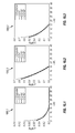
- Figures 15.1-15.3 are graphs 1500.1-1500.3 depicting pressure (p) (y-axis) versus time (t) (x-axis) for Fluids 1-3 of Table 1, respectively. These graphs show a comparison between the 2-D model and the 1-D numerical solution for injection of the various fluids listed in Table 1.
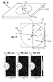
- FIG. 16 is a schematic diagram 1600 depicting parallel plates 1612 having an inlet 1614 therethrough.
- the computational grid or mesh
- Equation (49) the computational grid is not radially symmetric and may induce anisotropy despite attempts to ensure that fluid properties are isotropic (see Equation (49)).
- FIG. 17 is a schematic diagram 1700 depicting a 2-D computational domain simulating one symmetric half ( x > 0) of the full fracture domain of inlet 1614' bisected along a plane of symmetry P s and with injection at centerline C 0 .
- Lx radius r of the circular inlet 1714'.
- a low viscosity Newtonian fluid e.g., Fluid 0 in Table 1
- various Newtonian and non-Newtonian fluids e.g., Fluids 1 - 3 in Table 1 were injected at the center C 0 of left edge at a rate of 5 barrels per minute (corresponding to 10 barrels per minute in the full fracture).
- the fluid was injected into a region of the mesh 3 cells across.
- Figures 18.1-18.3 depict three graphs 1800.1-1800.3 showing simulations for each of the Fluids 1-3, respectively, passing through the bisected inlet 1614' of Figure 17 .
- Each of the three Fluids 1-3 were run out to 200 seconds and the resulting fluid fronts show excellent symmetry as shown in Figures 18.1-18.3 .
- These figures show 2-D simulation results at 200 seconds for injection of Fluids of Table 1.
- FIG. 19.1-19.3 depict graphs 1900.1-1900.3 of pressure p (y-axis) versus radius r (x-axis). These graphs 1900.1-1900.3 plot lines showing a comparison of the results of the 1-D with the 2-D simulations for injection of the Fluids 1-3 of Table 1 along the 0°, 45° and 90° directions (see Figure 17 ), respectively. As the simulations approach the injector, the simulations capture a singular behavior of the pressure field to differing degrees. In addition, there are minimal differences between pressure fields reported along the three different lines from the injector.
- This Section III provides another version 2056 of the method of generating proppant parameters 256.
- the method 2056 involves the same features 260, 262, 266, 268 and 269 as previously described.
- the predicting 264 aperture change for a prescribed closure stress using the linear asperity model has been modified to predict 2064 aperture change using nonlinear deformation.
- the method 2064 may involve predicting aperture change and conductivity using nonlinear deformation and may be performed using a numerical prediction and/or an analytical approach.
- Numerical predictions may be made using numerical models including spatial distribution of variations in aperture. Such predictions may be used to predict the evolution of fracture closure and hydraulic conductivity under stress. Analytic predictions may also be made by holding open deformation and conductivity of fractures by either natural (roughness) or artificial (e.g., proppant) mechanisms.
- the analytic approach seeks to honor the geometry of connectivity of the channels within the fracture while providing an efficient solution for fracture closure and fracture conductivity.
- the analytic approach seeks to captures nonlinear effects due to stiffening of the material holding the fracture open as well as the development of additional contact points within the channels.
- Fracture conductivity may be determined 266 as previously described, and/or as described further below in Section IV below.
- the method may be validated (verified) 269 as previously described, or as further described in Section V below.
- Validation 269 may involve, for example, comparison with numerical and analytic solutions to demonstrate good multi-threaded performance.
- nonlinear stiffening of the asperities may be considered using computational framework for pillars and channels between two half-spaces.
- the deformation model predicts both the reduction of fracture aperture and the nonlinear redistribution of stress due to pinch-points developing in the channels between pillars.
- the deformation model achieves a rapid solution through simplifications to the fracture geometry and through application of a preconditioner that reduces the number of iterations required.
- Fracture conductivity may be calculated on a Cartesian grid using the original distribution of aperture with changes in aperture prescribed according to the results of the mechanical model.
- Examples indicate verification of the behavior of the code against both analytic results and another simulator.
- the performance of the method may permit simulation of many hundreds of pillars/channels within many fractures in seconds. Comparisons with the higher fidelity model indicate the nonlinear extension model predicts the average aperture to within 5-10% and conductivity to within a factor of 2-4.
- the nonlinear extension model may be used to provide efficiency, and to facilitate more extensive parameter studies. Nonlinearity in the constitutive model of the pillars within a fracture including potential pillar spreading may also be provided. Future applications of the method may consider nonlinearity due to spreading and compaction of weak proppant pillars and embedment of proppant in weak formations.
- the hydraulic conductivity of fractures under stress may be of interest for a range of applications.
- the deformed state and associated hydraulic conductivity of natural and hydraulically-induced fractures at depth may be predicted. Examples of prediction are provided by R. Jung, Goodbye or Back to The Future, in Effective And Sustainable Hydraulic Fracturing, Proceedings of the International Conference For Effective and Sustainable Hydraulic Fracturing (HF2013), InTech, pp. 95-121, Brisbane, Australia, May 20-22 (2013 ), the entire contents of which is hereby incorporated by reference herein.
- artificial components such as proppant
- proppant may be introduced into hydraulic fractures in order to maintain conductivity under stress.
- artificial components such as proppant
- L. R. Kern T. K. Perkins, R. E. Wyant, The Mechanics Of Sand Movement In Fracturing, Transactions of the American Institute of Mining and Metallurgical Engineers 216 403-405 (1959 ); and C. Montgomery, Fracturing Fluids, Proceedings Of The Int'l Conf. For Effective And Sustainable Hydraulic Fracturing (HF2013), InTech, pp. 3-24, Brisbane, Australia, May 20-22 (2013 ), the entire contents of which are hereby incorporated by reference herein.
- some classes of proppant placement technology may involve attempting to induce heterogeneity in the arrangement of the proppant in order to create open flow channels within the propped fracture (heterogeneous proppant placement).
- heterogeneous proppant placement See, e.g., A. Medvedev, K. Yudina, M. K. Panga, C. C. Kraemer, A. Pena, On The Mechanisms Of Channel Fracturing, SPE 163836 ; and J. P. Morris, N. Chugunov, G. Meouchy, Understanding Heterogeneously Propped Hydraulic Fractures Through Combined Fluid Mechanics, Geomechanics, And Statistical Analysis, 48th U.S. Rock Mechanics/Geomechanics Symposium, Minneapolis, pp. 2014-7408, June 1-4, (2014 ) (referred to herein as "Morris (2014)”), the entire contents of which are hereby incorporated by reference herein.
- the fracture conductivity may be dominated by induced channelization within the fracture either due to the spatial distribution of aperture (in the case of natural fractures) or heterogeneity in the distribution of proppant (in the case of proppant placement during hydraulic fracturing).
- aperture in the case of natural fractures
- proppant in the case of proppant placement during hydraulic fracturing
- both experimental and modeling studies indicate that individual natural fractures exhibit an evolving network of channels under stress. See: L. J. Pyrak-Nolte, L. R. Myer, N. G. W. Cook, P. A. Witherspoon, Hydraulic And Mechanical Properties Of Natural Fractures In Low Permeability Rock, G. Herget, S.
- Solutions may be developed for the detailed deformation of fractures taking into account the spatial distribution of material within the fracture.
- a fracture with two parallel half-spaces separated by a spatial distribution of contacting points may be considered. See, e.g., J. A. Greenwood, J. B. P. Williamson, Contact Of Nominally Flat Surfaces, Proceedings of the Royal Society of London. Series A, Mathematical and Physical Sciences 295 (1442) (1966) 300-319 ; and S. Brown, C. Scholz, Closure Of Random Elastic Surfaces In Contact, Jnl. Of Geophysical Research-Solid Earth And Planets 90 5531-5545 (1985 ), the entire contents of which is hereby incorporated by reference herein.
- the contact regions as deformable pillars and including the interaction between the pillars may be treated by allowing each of the half-spaces to deform about the pillars.
- D. L. Hopkins The Effect Of Surface Roughness on Joint Stiffness, Aperture, And Acoustic Wave Propagation, Ph.D. Thesis, University of California at Berkeley (1990 ) (referred to herein as "Hopkins (1990)"), the entire contents of which is hereby incorporated by reference herein.
- the solutions may also involve considering a regular grid of small contact elements (referred to as asperities) and exploiting fast multipole methods. See, e.g., Purak-Nolte (2000).
- a combination of boundary elements may be used to simulate the rock matrix deformation with an asperity mechanical model to capture the detailed geometry and mechanical response of an arbitrary combination of pillars and channels. See, e.g., Purak-Nolte (2000) and Morris (2011).
- the deformation of mineralized pillars see, e.g., Morris (2011)
- heterogeneous arrangements ofproppant within a fracture may also be considered.
- Deformation of natural channels within a variable aperture fracture may be predicted using an asperity model. See, e.g., Pyrak-Nolte (2000).
- simulations may involve extensive computational requirements when considering highly subdiscretized pillars/channels.
- simulations may be provided with increased computational efficiency where the number of pillars and associated channels remains small. See, e.g., Hopkins (1990). Additional computational burden may be imposed in methods involving the use of a large number of asperities to sub-discretize the individual physical pillars and channels. More pillars and channels may lead to increased reliability of the model.
- the connectivity of the flow field may be altered by the incidental introduction of numerical artifacts that either create or remove channels from the model. Because the presence or absence of channels may affect hydraulic conductivity, changes in flow geometry may affect the predicted flow field within the fracture.
- a nonlinear extension approach may be used. As the resolution is increased, geomechanical calculations may use a majority of computational effort and the increased resolution may be needed for an accurate conductivity calculation.
- the hybrid approach involves solving the geomechanical deformation on a relatively coarse grid, while conductivity is calculated using a more refined discretization.
- the hybrid approach seeks to respect the geometry and connectivity of channels within the fracture (either natural or artificial), while changes in aperture due to stress are also included such that, for the same amount of computational effort, many more channels can be included within a single computation.
- Asperity models may be used involving a linear elastic constitutive response for the asperities. See, e.g., Pyrak-Nolte (2000), Morris (2011), and Morris (2014). Extensions to the models may be provided to allow for elastic, perfectly plastic behavior and/or to address material failure. See: P. Ameli, J. E. Elkhoury, J. P. Morris, R. L. Detwiler, Fracture Permeability Alteration Due to Chemical And Mechanical Processes: a Coupled Highresolution Model, Rock Mech Rock Eng., DOI 10.1007/s00603-014-0575-z (2014 ); and E. A. Ejofodomi, G. Cavazzoli, J. Morris, R.
- This nonlinear extension method may be similar to the nonlinear method of Figure 5.2 , except that the method of Figure 20 provides further detail on nonlinear deformation.
- the 2064 predicting aperture change and conductivity using nonlinear deformation involves converting 2066 the pillar/channel geometry into a simplified approximation, such as a cylindrical pillars or cylindrical representation (see Section 4.3), and determining 2068 deformation of the fracture (see Section 4.4).
- the converting 2066 may be performed using a mechanical approach involving pillar geometry, or using an analytical approach involving a cylinder approximation projection onto a Cartesian grid.
- the determining 2068 may be performed by generating deformation 2068.1 based on the cylindrical pillars (see Section 3.4.1), linearizing 2068.2 portions of the deformation of cylindrical pillars (see Section 3.4.2), assembling 2068.3 a linear system of responses of the cylindrical pillars (see Section 3.4.3), and considering 2068.4 pinch-points (see Section 3.4.4).
- the fracture conductivity 266 may then be determined (see Section IV). For additional pinch-points, the linearizing 2068.2, assembling 2068.3, and solving 2068.4 may be repeated.
- the method proceeds by progressively adding stress to the fracture in order to smoothly approach the requested stress level.
- the estimate represented by a nonlinear system of equations, is linearized (see Section 3.4.2) to obtain an iterative solution to the linear system, and to identify points of contact ("pinch-points") (see Section 3.4.4 below).
- the final fracture aperture and conductivity is calculated (see Section IV below).
- the accuracy of the conductivity prediction depends on the presence or absence of channels within the heterogeneous distribution ofproppant or natural roughness.
- To accelerate the geomechanical calculation relatively few, simple computational elements (cylindrical pillars) are used. In the process of approximating the channel geometry with coarser pillars, spurious channels may be introduced or removed.
- Figures 21 and 22 are schematic diagrams depicting models 2100.1, 2100.2 lacking a channel and adding a channel, respectively. These figures present two scenarios where the conversion to cylinders may introduce errors into the conductivity estimation.
- the initial pillar geometry includes pillars 2102.1 containing a narrow channel 2104.1 that is removed in the conversion to a cylindrical representation 2102.1'.
- the initial pillar geometry includes two neighboring pillars 2102.1 with a neck of material 2104.2 spanning the gap between them.
- the conversion to cylindrical approximation 2102.2' removes the material 2104.2 from the gap, creating a spurious channel.
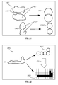
- Figure 22 is a schematic diagram depicting a model using multiple internal representations of pillars/channels.
- a true (arbitrary) proppant pillar shape 2206 is provided.
- An approximation with cylinders 2208.1 and a projection onto a Cartesian (flow) grid 2208.2 are generated.
- the cylinder approximation 2208.1 may be a fast geomechanical representation.
- the projection 2208.2 may be a conductivity representation that honors geometry and/or channels.
- the multiple internal representations include a mechanical representation that makes simplifying assumptions regarding the pillar/channel geometry (i.e.: cylinders) in order to achieve a rapid solution, and an analytical representation using a Cartesian grid to capture the pillar/channel geometry as accurately as possible for the conductivity calculation.
- the mechanical representation may involve making simplifying assumptions regarding the spatial distribution of the pillars and their geometry in order to achieve a rapid solution.
- the analytical representation may use a more detailed grid to capture the channel geometry as accurately as possible for the conductivity calculation.
- changes in aperture may be communicated from the geomechanical representation 2208.1 to the Cartesian grid 2208.2.
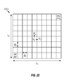
- Changes in aperture predicted by the geomechanical calculation may be communicated to the Cartesian grid as shown in the schematic diagram of Figure 23 .
- the Cartesian grid 2202 defines a plurality of rectangles (called cells), each having a width ⁇ x and a length ⁇ y.
- the overall dimensions of the grid are L x by L y and with each cell having a pressure p ij with fluxes q ij x and q ij y .
- the Cartesian grid 2208.2 may be used for calculating fluid flow. Pressures p ij are cell-centered, while fluxes q ij x and q ij y are face-centered. In this way, the mechanical deformation may be predicted without introducing changes to the channel connectivity.
- Fracture deformation 2068 may be performed using the techniques described with respect to the method of Figure 5.2 .
- the fracture deformation 2068 may be involve determining 582 cylinder and half-space deformation consistent with applied stress, and/or an extension thereof.
- the surrounding formation may be modeled with two half-spaces. It is also assumed that both the pillars and formation can deform nonlinearly to capture combinations of elastic and plastic effects. To simplify the calculation, that nonlinear effects in the formation are assumed to be localized to a zone that is comparable to the initial aperture of the fracture. Consequently, the far-field interactions between the pillars may be taken to be linearly elastic. The localized nonlinear deformation of the formation at pillar I and the deformation of pillar I itself are lumped into a deformed height of pillar l I .
- the average deformed height of each individual pillar, l I may be consistent with an average aperture of the fracture at the location of the pillar.
- the local aperture is the sum of the unperturbed half-space gap, D, and the contributions to the local deformation due to forcing from all pillars.
- the quantity D is the separation of the elastic half-spaces in the absence of any pillars to hold them apart. As D is decreased, the forces induced upon the pillars increase. The value of D that induces the prescribed level of stress within the fracture is to be found.
- C lI is a constant that captures the linear dependence of pillar width change with stress and the superscript 0 indicates some reference state.
- C faI is a constant that can be obtained through expansion of f I / a I using the initial slope of a I .
- Equation (66) may be rewritten as follows: ⁇ ⁇ D + ⁇ J ⁇ I W IJ ⁇ ⁇ ⁇ f J + ⁇ ⁇ 1 - ⁇ 2
- ⁇ nI M I ⁇ ⁇ nI
- ⁇ n I f I ⁇ ⁇ a I 2
- nI l I 0 - l I l I 0
- M I l I 0 M I ⁇ ⁇ a I 2 ⁇ f I
- C lI - l I 0 M I ⁇ ⁇ ⁇ a I 2 specifically for the case of a linear elastic pillar.
- the method provided herein remains general and considers the nonlinear case.
- Equation (76) an iterative solution is provided utilizing solutions from the previous nonlinear step as the initial guess for the solution of each subsequent iteration.
- the system of equations described by Equation (76) may be considered dense and with reduced conditioning.
- Pinch-points may be added using the techniques described with respect to Figure 5.2 and/or as further described in this section. For each additional pinch-point detected, portions of the methods 256 of Figure 5.2 and/or 2056 of Figure 20 may be repeated.
- pinch-points As the stress applied to the channels within the fracture is increased, it is possible for fracture surfaces within the open channels to make contact at "pinch-points." The presence of such pinch-points may reduce the conductivity within the fracture. Such pinch-points may also carry stress, leading to nonlinearity. If the stress carried by the pinch-points is neglected, the pillars alone carry the load, and the channels may close prematurely. At high stress levels, fractions of the total load may be taken up by such pinch-points. As a consequence, methods that neglect pinch-point mechanics may underestimate the conductivity of the stressed fracture.
- Pinch-point mechanics may be accommodated by treatment as virtual pillars that are introduced into the stress calculation if contact is detected at their location.
- a list of potential pinch-points to be monitored on a regular grid may be identified.
- the spacing of the pinch-points may be chosen automatically based upon the size of the pillars (e.g., sized such that 5 pinch-points span the average pillar size). Any candidate pinch-points that happen to fall within an existing pillar may be deleted from the list.
- the pinch-point mechanics may involve creating a list of pinch-points, incrementally providing stress, determining deformation 2068 with the list of pinch-points, adjusting (e.g., adding/removing) pinch-points, remove any pinch-points found to be in tension, sorting a list of points of overlap from largest to smallest, adding a portion of locations at the points of overlap to the list of pinch-points in order of greatest overlap to smallest overlap, repeating the incrementally providing stress until the target stress level is reached.
- the pinch-point mechanics proceeds by repeating the 2068.2 linearizing, 2068.3 assembling, and 2068.4 solving (see, e.g., Section 3.4.2 above) for each pinch-point.
- the fracture conductivity may be determined 266 as described with respect to Figures 2-6 . These approaches involve obtaining the deformed pillar states ( l I , a I , f I ) and the resultant deformed fracture aperture at a set of arbitrary points within the fracture. A means for determining 266 the hydraulic conductivity of the deformed fracture ( Figure 20 ) may also involve solving flow in the fracture using fully 3-D numerical techniques. In cases where reduced computational cost is needed, a lubrication approximation within the fracture and reduce the dimensionality of the numerical solution to 2-D may be performed. See, e.g., Pyrak-Nolte (2000) and Section 3.4.3 above.
- the right-going and up-going volumetric fluxes (units of volume per unit time) from cell i, j are defined on the faces of the cells (see Figure 23 ) and are denoted by q ij x and q ij y , respectively.
- a solution for the pore pressure field can be obtained by requiring conservation of fluid mass within the fracture while flow is induced between an inlet and outlet pressure boundary condition.
- q ij y c ij y ⁇ p ij - p ij + 1 where the conductivities, c x ij and c y ij depend upon what occupies the cell in question.
- the conductivity is taken to be an approximation for flow between two plates. If the cell is within a proppant pillar, it is treated as a porous medium, and the conductivity is calculated using Darcy's law. If the pillar represents solid rock, the cell is ascribed an arbitrarily low permeability. See, e.g., Morris (2014).
- c ij y ⁇ ⁇ x ⁇ w ij y 3 12 ⁇ ⁇ ⁇ 1 ⁇ ⁇ y
- the face fluxes can be calculated from (100,101) and then the total inlet and outlet fluxes can be calculated. From these total fluxes, fracture conductivity can be inferred.
- Validation may be determined 269 as described with respect to Figures 2-6 . Validation may also be performed using the methods described in Sections III and IV. Validation 269 may be performed to verify the fracture conductivity determined 266. Validation may also be performed to verify the methods used during simulation. Examples of validations are provided.
- Table 4 provides a comparison between the analytic solution for flow between two plates using the discretization described in Table 3. Less than 0.01% error between the code and the analytic solution is observed, suggesting that the implementation is accurate for both non-square domains and non-square flow elements.
- Table 4 below indicates that the results agree to 6 significant figures, suggesting the implementation of flow through a porous pack even for high aspect ratio elements and computational domains: TABLE 4 Numerical (m 3 /s) Analytic (m 3 /s) Rel. Error Qx 3.5082 ⁇ 10 -9 3.5082 ⁇ 10 -9 ⁇ 0.003% Qy 6.35287 ⁇ 10 -10 6.35287 ⁇ 10 -6 ⁇ 0.003% Table 4 provides a comparison between code and analytic solution for flow between two plates propped homogeneously with 300 D permeable material (e.g., proppant) using the discretization described in Table 3.
- 300 D permeable material e.g., proppant
- Figure 24.1 is a schematic diagram depicting a fracture 2412.1 showing the heterogeneous proppant 2414.1 arrangement considered for flow convergence study.
- Table 5 below compares the predicted conductivity for a range of discretizations of the fracture.
- Validations 269 may be performed to compare various methods used herein. Such validations may involve a comparison of one or more of the simulations and/or results provided herein.
- Simulation using the analytical method may be compared against a more detailed "asperity" model that has itself been verified against numerous analytic solutions. See, e.g., Morris (2014) and Pyrak-Nolte (2000).
- the choice of ⁇ may be made to match that assumed internally by the asperity model.
- the asperity model mesh used the grid size of 0.5 m, while our fast-running model used a pillar radius of 0.282095 m to obtain pillars with the same area as the 0.5 m by 0.5 m asperities.
- Table 7 below depicts relative error between an asperity model and the method provided herein for three verification problems 1-3. TABLE 7 Problem Average error Max error 1 0.12% 1.5% 2 0.80% 3.6% 3 0.25% 1.5% The asperity model uses a more precise functional form for the deformation rather than the far-field approximation. Consequently, the greatest errors are at points close to the pillar. Table 7 reports the relative error between the simulations indicating that on average less than 0.1 % error is obtained, and indicates that the maximum error is 1.5 %.
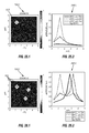
- the asperity model is shown in Figure 25.1 along with the comparison between the two approaches as shown in Figure 25.2 .
- Figure 25.1 is a graph 2500.1 having dimensions y(m) (y-axis) versus x(m) (x-axis) and depicting an asperity-based point 2516 of contact for the first verification problem.
- Figure 25.2 is a graph 2500.2 depicting aperture (mm) (y-axis) versus x(m) (x-axis).
- the asperity model is shown in Figure 26.1 along with the comparison between the two models as shown in Figure 26.2 .
- Figure 26.1 is a graph 2600.1 having dimensions y(m) (y-axis) versus x(m) (x-axis) and depicting an asperity points 2616 of contact for the second verification problem.
- Figure 26.2 is a graph 2600.2 depicting aperture (mm) (y-axis) versus x(m) (x-axis).
- a third verification problem considers the same three pillars with varied their heights to further test the nonlinear extension model.
- the pillars located at ( x,y ) (1.25,3.75), (3.25,3.25), and (2.75,1.75) were given heights of 4 mm, 5 mm, and 5.5 mm, respectively, and were subjected 2 MPa closure stress.
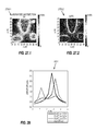
- Figures 27.1 and 27.2 The asperity computational model is shown in Figures 27.1 and 27.2 along with the comparison between the two models.
- Figure 27.1 is a graph 2700.1 having y(m) (y-axis) versus x(m) (x-axis) depicting a comparison between high-resolution asperity simulations having average aperture of 2.07 mm and conductivity of 58.3 D ⁇ m.
- Figure 27.2 is a graph 2700.2 having y(m) (y-axis) versus x(m) (x-axis) depicting the nonlinear extension model predictions of aperture distribution having an average aperture of 1.97 mm and conductivity of 25.9 D ⁇ m) within a fracture with non-trivial pillar geometries.
- the graphs 2700.1, 2700.2 indicate agreement between the two predictions of aperture change within the channel regions.
- the nonlinear extension model shows agreement with the asperity model for the expected portions of the domain and elsewhere the discrepancies are within several percent relative error.
- the asperity-based approach represents the proppant using a Cartesian grid for both flow and conductivity. See, e.g., Pyrak-Nolte (2000).
- the nonlinear extension method using cylinders for geomechanics and grid for flow is compared against a finely meshed asperity simulation for more general pillar geometries. The results of the comparison shown in Figure 28 indicate the two methods are in agreement.
- Figure 28 is a graph 2800 depicting a comparison between the two models of Figures 27.1 and 27.2.
- Figure 28 depicts a comparison between the asperity model and the nonlinear extension model for several different line outs within the domain for verification problem 3.
- Tables 8 and 9 below show simulation parameters, including mechanical and geometrical properties of the fracture, used for general pillar geometry verification problem (Section 5.2.1 above).
- TABLE 8 E 30.0e9 ⁇ 0.25 ⁇ 1.0 L x 40.0 L y 40.0 M I 300 MPa ⁇ n 2.5 MPa
- TABLE 9 Aperture (mm) Conductivity (D ⁇ m) Asperity model 1.1 19 Nonlinear extension model without pinch-points 0.71 0.0012 Nonlinear extension model with pinch-points 0.90 4.6
- the asperity simulation predicted a final average aperture of 2.07 mm, versus our model prediction of 1.97 mm.
- the asperity simulation predicted a conductivity of 58.3 D ⁇ m in contrast with the new fast-running prediction of 25.9 D ⁇ m.
- the average aperture is accurate to within approximately 5% while the conductivity agrees to within about a factor of 2.
- the conductivity calculation is sensitive to slight changes in aperture or geometry, indicating that agreement acceptable.
- Pinch-point mechanics may be accommodated via fine discretization of the fracture surfaces and contact detection. See, Pyrak-Nolte (2000).
- the change in aperture predicted by the nonlinear extension approach with and without pinch-points is compared with the asperity-based approach in Figures 29.1-29.3 for two pillars subjected to stress sufficient to partially close the channels between.
- Figures 29.1-29.3 are graphs 2900.1-2900.3 having y(m) (y-axis) versus x(m) (x-axis) depicting a comparison between high-resolution asperity simulation having average aperture of 2.07 mm and conductivity of 58.3 D ⁇ m.
- Figure 29.1 shows a high-resolution asperity-based simulation (1.1 mm average aperture and 19 D ⁇ m conductivity)
- Figure 29.2 shows a nonlinear extension model without pinch-points (0.71 mm average aperture and 0.0012 D ⁇ m conductivity)
- Figure 29.3 shows a nonlinear extension model with pinch-points (0.9 mm average aperture and 4.6 D ⁇ m conductivity).
- Table 10 shows simulation parameters including mechanical and geometrical properties of the fracture used for a pinch-point verification problem.
- Table 10 shows the numerical results of the calculations. In this example, neglecting pinch-points led to a 5 order reduction in the predicted conductivity compared with the asperity-based approach.
- Table 11 provides a comparison between the asperity model and the nonlinear extension model developed for the pinch-point test. TABLE 11 E 30 GPa ⁇ 0.25 ⁇ 1.0 Lx 100.0 m Ly 30.0 m aI 2.0 m 1I 5 mm MI 230 MPa pillar spacing 3.0 m ⁇ n 1 MPa By including pinch-points within approximately a factor of 4 of the asperity-based prediction, the conductivity calculation may be sensitive to slight changes in aperture or geometry. Consequently, this level of difference may be deemed acceptable.
- Efficiency of the various models may be compared.
- code used in the various simulations may be parallelized via multithreading, such as OpenMP multithreading.
- the model may be applied to many (potentially hundreds) of separate fractures containing tens or hundreds of pillars/channels.
- the calculations for each fracture may be treated separately and implemented in a thread-safe manner.
- Asperity methods may consider entirely arbitrary combinations of pillar geometry with fracture roughness and detailed additional points of contact under stress. See, e.g., Pyrak-Nolte (2000) and Morris (2014). Ten or more asperity elements may be used across a single pillar or channel to capture the mechanical deformation. Models may use more limited internal discretization of the pillars, and may be more efficient than the asperity-based approach for the case of circular pillars.
- the performance of the deformation calculation using the nonlinear extension model of the present disclosure may be compared with an asperity model (see, e.g., Morris (2014)) for a single fracture containing 330 circular pillars. Both models may be run single-threaded to simplify the performance comparison on a 2.4 GHz core.
- the asperity model takes over 40 minutes.
- the cost of the asperity calculation is roughly proportional to the square of the number of elements.
- the nonlinear extension method takes approximately 0.1 s.
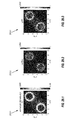
- the nonlinear extension model in single-threaded mode was used to simulate the three HPP geometries shown in Figures 30.1-30.3 .
- These figures provide graphs 3000.1-3000.3 containing 100, 400 and 900 pillars, respectively, within a single fracture.
- Figures 30.1-30.3 depict heterogeneous proppant pillar arrangements considered by the code performance study.
- composition used/disclosed herein can also comprise some components other than those cited.
- each numerical value should be read once as modified by the term "about” (unless already expressly so modified), and then read again as not so modified unless otherwise indicated in context.
- a concentration range listed or described as being useful, suitable, or the like is intended that any and every concentration within the range, including the end points, is to be considered as having been stated.
- a range of from 1 to 10 is to be read as indicating each and every possible number along the continuum between about 1 and about 10.
Landscapes
- Engineering & Computer Science (AREA)
- Geology (AREA)
- Life Sciences & Earth Sciences (AREA)
- Mining & Mineral Resources (AREA)
- Physics & Mathematics (AREA)
- Geochemistry & Mineralogy (AREA)
- Fluid Mechanics (AREA)
- General Life Sciences & Earth Sciences (AREA)
- Environmental & Geological Engineering (AREA)
- Theoretical Computer Science (AREA)
- Computer Hardware Design (AREA)
- Evolutionary Computation (AREA)
- Geometry (AREA)
- General Engineering & Computer Science (AREA)
- General Physics & Mathematics (AREA)
- Management, Administration, Business Operations System, And Electronic Commerce (AREA)
- Investigating Strength Of Materials By Application Of Mechanical Stress (AREA)
Applications Claiming Priority (2)
| Application Number | Priority Date | Filing Date | Title |
|---|---|---|---|
| US201361870901P | 2013-08-28 | 2013-08-28 | |
| US14/460,654 US9677393B2 (en) | 2013-08-28 | 2014-08-15 | Method for performing a stimulation operation with proppant placement at a wellsite |
Publications (2)
| Publication Number | Publication Date |
|---|---|
| EP2843184A2 true EP2843184A2 (de) | 2015-03-04 |
| EP2843184A3 EP2843184A3 (de) | 2016-01-06 |
Family
ID=51392166
Family Applications (1)
| Application Number | Title | Priority Date | Filing Date |
|---|---|---|---|
| EP14182269.2A Withdrawn EP2843184A3 (de) | 2013-08-28 | 2014-08-26 | Verfahren zur Durchführung einer Stimulationsoperation mit Stützmittelplatzierung an einem Bohrplatz |
Country Status (6)
| Country | Link |
|---|---|
| US (1) | US9677393B2 (de) |
| EP (1) | EP2843184A3 (de) |
| CN (1) | CN104695932A (de) |
| AU (1) | AU2014216034B2 (de) |
| CA (1) | CA2860662C (de) |
| RU (1) | RU2658968C2 (de) |
Cited By (2)
| Publication number | Priority date | Publication date | Assignee | Title |
|---|---|---|---|---|
| CN110390152A (zh) * | 2019-07-15 | 2019-10-29 | 中国矿业大学 | 一种模拟巷道围岩裂隙演化的离散元方法 |
| CN112145142A (zh) * | 2020-09-04 | 2020-12-29 | 四机赛瓦石油钻采设备有限公司 | 一种压裂井场三维部署系统 |
Families Citing this family (35)
| Publication number | Priority date | Publication date | Assignee | Title |
|---|---|---|---|---|
| US10001000B2 (en) * | 2013-07-22 | 2018-06-19 | Halliburton Energy Services, Inc. | Simulating well system fluid flow based on a pressure drop boundary condition |
| US9726001B2 (en) | 2013-08-28 | 2017-08-08 | Schlumberger Technology Corporation | Method for adaptive optimizing of heterogeneous proppant placement under uncertainty |
| GB2533847B (en) * | 2014-11-06 | 2017-04-05 | Logined Bv | Local layer geometry engine with work zone generated from buffer defined relative to a wellbore trajectory |
| CA2961562C (en) * | 2014-11-19 | 2018-07-31 | Halliburton Energy Services, Inc. | Formation fracture flow monitoring |
| US9990588B2 (en) * | 2015-03-19 | 2018-06-05 | Hitachi, Ltd. | System for predicting amount of production and method for predicting amount of production |
| US10365200B2 (en) * | 2015-05-22 | 2019-07-30 | Saudi Arabian Oil Company | Method for determining unconventional liquid imbibition in low-permeability materials |
| US10423736B2 (en) * | 2015-08-28 | 2019-09-24 | University Of British Columbia | Methods and systems for simulating hydrodynamics in gas-solid fluidized beds |
| RU2613689C1 (ru) * | 2016-02-24 | 2017-03-21 | Публичное акционерное общество "Татнефть" имени В.Д. Шашина | Способ гидравлического разрыва продуктивного пласта с глинистым прослоем и газоносным горизонтом |
| RU2618545C1 (ru) * | 2016-02-26 | 2017-05-04 | Публичное акционерное общество "Татнефть" имени В.Д. Шашина | Способ гидравлического разрыва пласта |
| RU2618544C1 (ru) * | 2016-03-03 | 2017-05-04 | Публичное акционерное общество "Татнефть" имени В.Д. Шашина | Способ гидравлического разрыва продуктивного пласта с глинистым прослоем и газоносным горизонтом |
| WO2017216594A1 (en) * | 2016-06-15 | 2017-12-21 | Schlumberger Technology Corporation | Induced seismicity |
| WO2018052950A1 (en) * | 2016-09-13 | 2018-03-22 | Proppant Express Solutions, Llc | Proppant tracking system |
| CN106837290B (zh) * | 2017-02-14 | 2019-03-15 | 中国石油大学(北京) | 对称式布缝的分组异井异步注co2采油方法 |
| US10914139B2 (en) * | 2017-02-22 | 2021-02-09 | Weatherford Technology Holdings, Llc | Systems and methods for optimization of the number of diverter injections and the timing of the diverter injections relative to stimulant injection |
| US10612356B2 (en) | 2017-03-01 | 2020-04-07 | Proptester, Inc. | Fracture fluid and proppant transport testing systems and methods of using same |
| US11365626B2 (en) * | 2017-03-01 | 2022-06-21 | Proptester, Inc. | Fluid flow testing apparatus and methods |
| US12228026B2 (en) | 2017-09-14 | 2025-02-18 | Saudi Arabian Oil Company | Modeling reservoir permeability through estimating natural fracture distribution and properties |
| CA3080938C (en) * | 2017-11-01 | 2022-12-13 | Seismos, Inc. | Fracture length and fracture complexity determination using fluid pressure waves |
| CN108397184B (zh) * | 2018-05-18 | 2021-04-20 | 西南石油大学 | 一种自支撑裂缝导流能力的数值计算方法 |
| CN111305806B (zh) * | 2018-11-27 | 2022-06-03 | 中国石油天然气股份有限公司 | 自支撑裂缝导流能力的分析方法及装置 |
| WO2020242615A1 (en) | 2019-05-31 | 2020-12-03 | Exxonmobil Upstream Research Company | Modeling fluid flow in a wellbore for hydraulic fracturing pressure determination |
| CN110306971A (zh) * | 2019-07-01 | 2019-10-08 | 中国石油天然气股份有限公司大港油田分公司 | 一种高含水后期油藏流场分级评价方法 |
| US20230034507A1 (en) * | 2019-12-19 | 2023-02-02 | Schlumberger Technology Corporation | Formation stimulation with acid etching model |
| CN112761609B (zh) * | 2021-02-19 | 2022-02-01 | 西南石油大学 | 一种水力压裂作业中高效铺置支撑剂的优化方法 |
| CN113360984B (zh) * | 2021-06-08 | 2022-03-11 | 西南石油大学 | 一种考虑壁面捕获效应的支撑剂输送数值模拟方法 |
| US11525935B1 (en) | 2021-08-31 | 2022-12-13 | Saudi Arabian Oil Company | Determining hydrogen sulfide (H2S) concentration and distribution in carbonate reservoirs using geomechanical properties |
| US11921250B2 (en) | 2022-03-09 | 2024-03-05 | Saudi Arabian Oil Company | Geo-mechanical based determination of sweet spot intervals for hydraulic fracturing stimulation |
| US12560741B2 (en) | 2022-04-04 | 2026-02-24 | Saudi Arabian Oil Company | System and method to develop naturally fractured hydrocarbon reservoirs using a fracture density index |
| CN114645700B (zh) * | 2022-04-20 | 2023-07-18 | 中国矿业大学 | 一种强塑性材料灌装高压水致裂裂隙岩体的方法 |
| US11867047B2 (en) | 2022-06-08 | 2024-01-09 | Saudi Arabian Oil Company | Workflow to evaluate the time-dependent proppant embedment induced by fracturing fluid penetration |
| CN115199238B (zh) * | 2022-09-15 | 2022-11-25 | 四川省贝特石油技术有限公司 | 一种用于气藏开采的微细暂堵剂投放控制方法及系统 |
| WO2025064746A1 (en) * | 2023-09-20 | 2025-03-27 | University Of Wyoming | Rough-walled fractures, forming proppant-packed assemblies, processes of forming, and uses thereof |
| US12312951B1 (en) | 2024-04-26 | 2025-05-27 | Saudi Arabian Oil Company | Fracture reactivation index (FRI) for seal integrity analysis in carbon capture and storage (CCS) |
| US12493137B1 (en) | 2024-06-11 | 2025-12-09 | Saudi Arabian Oil Company | Building natural fractures model using 3D stacked geological models |
| CN119720609B (zh) * | 2025-02-27 | 2025-04-25 | 西南石油大学 | 一种砾岩油藏凝胶-二氧化碳交替驱替临界压力梯度的确定方法 |
Citations (12)
| Publication number | Priority date | Publication date | Assignee | Title |
|---|---|---|---|---|
| US6101447A (en) | 1998-02-12 | 2000-08-08 | Schlumberger Technology Corporation | Oil and gas reservoir production analysis apparatus and method |
| US6776235B1 (en) | 2002-07-23 | 2004-08-17 | Schlumberger Technology Corporation | Hydraulic fracturing method |
| US7363162B2 (en) | 2003-11-25 | 2008-04-22 | Schlumberger Technology Corporation | Gas reservoir evaluation and assessment tool method and apparatus and program storage device |
| US20080133186A1 (en) | 2006-12-04 | 2008-06-05 | Chevron U.S.A. Inc. | Method, System and Apparatus for Simulating Fluid Flow in a Fractured Reservoir Utilizing A Combination of Discrete Fracture Networks and Homogenization of Small Fractures |
| US7451812B2 (en) | 2006-12-20 | 2008-11-18 | Schlumberger Technology Corporation | Real-time automated heterogeneous proppant placement |
| US7581590B2 (en) | 2006-12-08 | 2009-09-01 | Schlumberger Technology Corporation | Heterogeneous proppant placement in a fracture with removable channelant fill |
| US20100138196A1 (en) | 2008-12-03 | 2010-06-03 | Chevron U.S.A. Inc. | System and method for predicting fluid flow characteristics within fractured subsurface reservoirs |
| US7788074B2 (en) | 2004-08-30 | 2010-08-31 | Institut Francais Du Petrole | Method of modelling the production of an oil reservoir |
| US20100250215A1 (en) | 2009-03-30 | 2010-09-30 | Object Reservoir, Inc. | Methods of modeling flow of gas within a reservoir |
| US20120179444A1 (en) | 2007-01-29 | 2012-07-12 | Utpal Ganguly | System and method for performing downhole stimulation operations |
| US8412500B2 (en) | 2007-01-29 | 2013-04-02 | Schlumberger Technology Corporation | Simulations for hydraulic fracturing treatments and methods of fracturing naturally fractured formation |
| US8584755B2 (en) | 2006-01-27 | 2013-11-19 | Schlumberger Technology Corporation | Method for hydraulic fracturing of subterranean formation |
Family Cites Families (12)
| Publication number | Priority date | Publication date | Assignee | Title |
|---|---|---|---|---|
| US4828028A (en) | 1987-02-09 | 1989-05-09 | Halliburton Company | Method for performing fracturing operations |
| US7496488B2 (en) | 2003-03-06 | 2009-02-24 | Schlumberger Technology Company | Multi-scale finite-volume method for use in subsurface flow simulation |
| US7398829B2 (en) * | 2006-09-18 | 2008-07-15 | Schlumberger Technology Corporation | Methods of limiting leak off and damage in hydraulic fractures |
| JP2008077209A (ja) | 2006-09-19 | 2008-04-03 | Ricoh Co Ltd | 機器管理方法及び機器管理システム |
| US9085727B2 (en) | 2006-12-08 | 2015-07-21 | Schlumberger Technology Corporation | Heterogeneous proppant placement in a fracture with removable extrametrical material fill |
| RU2349740C2 (ru) * | 2007-04-10 | 2009-03-20 | Владимир Александрович Афанасьев | Способ разработки нефтяного месторождения |
| US8014987B2 (en) * | 2007-04-13 | 2011-09-06 | Schlumberger Technology Corp. | Modeling the transient behavior of BHA/drill string while drilling |
| CA2738122C (en) * | 2008-09-19 | 2020-02-11 | Chevron U.S.A. Inc. | Computer-implemented systems and methods for use in modeling a geomechanical reservoir system |
| RU2412454C2 (ru) * | 2009-05-04 | 2011-02-20 | Федеральное государственное унитарное предприятие Сибирский научно-исследовательский институт геологии, геофизики и минерального сырья | Способ обработки сейсмических данных с использованием дискретного вейвлет-преобразования |
| RU2455665C2 (ru) * | 2010-05-21 | 2012-07-10 | Шлюмбергер Текнолоджи Б.В. | Способ диагностики процессов гидроразрыва пласта в режиме реального времени с использованием комбинирования трубных волн и микросейсмического мониторинга |
| US20120156787A1 (en) * | 2010-12-15 | 2012-06-21 | Saudi Arabian Oil Company | Laboratory Testing Procedure to Select Acid or Proppant Fracturing Stimulation Treatment for a Given Carbonate Formation |
| CN102174883B (zh) | 2011-01-13 | 2013-05-29 | 东北石油大学 | 清水压裂自支撑裂缝导流能力测试方法 |
-
2014
- 2014-08-15 US US14/460,654 patent/US9677393B2/en active Active
- 2014-08-22 AU AU2014216034A patent/AU2014216034B2/en active Active
- 2014-08-25 RU RU2014134639A patent/RU2658968C2/ru active
- 2014-08-26 EP EP14182269.2A patent/EP2843184A3/de not_active Withdrawn
- 2014-08-27 CA CA2860662A patent/CA2860662C/en active Active
- 2014-08-28 CN CN201410649142.0A patent/CN104695932A/zh active Pending
Patent Citations (14)
| Publication number | Priority date | Publication date | Assignee | Title |
|---|---|---|---|---|
| US6101447A (en) | 1998-02-12 | 2000-08-08 | Schlumberger Technology Corporation | Oil and gas reservoir production analysis apparatus and method |
| US6776235B1 (en) | 2002-07-23 | 2004-08-17 | Schlumberger Technology Corporation | Hydraulic fracturing method |
| US7363162B2 (en) | 2003-11-25 | 2008-04-22 | Schlumberger Technology Corporation | Gas reservoir evaluation and assessment tool method and apparatus and program storage device |
| US7788074B2 (en) | 2004-08-30 | 2010-08-31 | Institut Francais Du Petrole | Method of modelling the production of an oil reservoir |
| US8584755B2 (en) | 2006-01-27 | 2013-11-19 | Schlumberger Technology Corporation | Method for hydraulic fracturing of subterranean formation |
| US20080133186A1 (en) | 2006-12-04 | 2008-06-05 | Chevron U.S.A. Inc. | Method, System and Apparatus for Simulating Fluid Flow in a Fractured Reservoir Utilizing A Combination of Discrete Fracture Networks and Homogenization of Small Fractures |
| US8066068B2 (en) | 2006-12-08 | 2011-11-29 | Schlumberger Technology Corporation | Heterogeneous proppant placement in a fracture with removable channelant fill |
| US7581590B2 (en) | 2006-12-08 | 2009-09-01 | Schlumberger Technology Corporation | Heterogeneous proppant placement in a fracture with removable channelant fill |
| US8490700B2 (en) | 2006-12-08 | 2013-07-23 | Schlumberger Technology Corporation | Heterogeneous proppant placement in a fracture with removable channelant fill |
| US7451812B2 (en) | 2006-12-20 | 2008-11-18 | Schlumberger Technology Corporation | Real-time automated heterogeneous proppant placement |
| US20120179444A1 (en) | 2007-01-29 | 2012-07-12 | Utpal Ganguly | System and method for performing downhole stimulation operations |
| US8412500B2 (en) | 2007-01-29 | 2013-04-02 | Schlumberger Technology Corporation | Simulations for hydraulic fracturing treatments and methods of fracturing naturally fractured formation |
| US20100138196A1 (en) | 2008-12-03 | 2010-06-03 | Chevron U.S.A. Inc. | System and method for predicting fluid flow characteristics within fractured subsurface reservoirs |
| US20100250215A1 (en) | 2009-03-30 | 2010-09-30 | Object Reservoir, Inc. | Methods of modeling flow of gas within a reservoir |
Non-Patent Citations (20)
| Title |
|---|
| A. MEDVEDEV; K. YUDINA; M. K. PANGA; C. C. KRAEMER; A. PENA: "On The Mechanisms Of Channel Fracturing", SPE 163836 |
| C. MONTGOMERY: "Fracturing Fluids", PROCEEDINGS OF THE INT'L CONF. FOR EFFECTIVE AND SUSTAINABLE HYDRAULIC FRACTURING (HF2013), INTECH, 20 May 2013 (2013-05-20), pages 3 - 24 |
| CHHABRA, R. P.; RICHARDSON, J. F.: "Non-Newtonian Flow And Applied Rheology: Engineering Applications", 2008, ELSEVIER |
| D. L. HOPKINS: "The Effect Of Surface Roughness on Joint Stiffness, Aperture, And Acoustic Wave Propagation", PH.D. THESIS, 1990 |
| DRAZER, G.; J. KOPLIK: "Permeability of Self-Affine Rough Fractures", PHYSICAL REVIEW E, vol. 62, no. 6, 2000, pages 8076 - 8085 |
| E. A. EJOFODOMI; G. CAVAZZOLI; J. MORRIS; R. PRIOUL: "Application Of Channel Fracturing In The Vaca Muerta Shale Formation", SPE LATIN AMERICAN AND CARIBBEAN PETROLEUM ENGR. CONF., 21 May 2014 (2014-05-21) |
| H. A. VAN DER VORST: "Bi-cgstab: A Fast And Smoothly Converging Variant of Bi-Cg For The Solution OfNonsymmetric Linear Systems", SIAM J. SCI. STAT. COMPUT., vol. 13, no. 2, 1992, pages 631644, XP008116935, DOI: doi:10.1137/0913035 |
| HARLOW, F.H.: "A Machine Calculation Method for Hydrodynamic Problems", LOS ALAMOS SCIENTIFIC LABORATORY REPORT LAMS-1956, 1955 |
| J. A. GREENWOOD; J. B. P. WILLIAMSON: "Contact Of Nominally Flat Surfaces", PROCEEDINGS OF THE ROYAL SOCIETY OF LONDON. SERIES A, MATHEMATICAL AND PHYSICAL SCIENCES, vol. 295, no. 1442, 1966, pages 300 - 319 |
| J. P. MORRIS; J. W. JOHNSON: "Predicting The Long-Term Evolution Of Fracture Transport Properties in Co2 Sequestration Systems, US Rock Mechanics/Geomechanics Symposium", ARMA, 26 June 2011 (2011-06-26), pages 11 - 399 |
| J. P. MORRIS; N. CHUGUNOV; G. MEOUCHY: "Understanding Heterogeneously Propped Hydraulic Fractures Through Combined Fluid Mechanics, Geomechanics, And Statistical Analysis", 48TH U.S. ROCK MECHANICS/GEOMECHANICS SYMPOSIUM, 1 June 2014 (2014-06-01), pages 2014 - 7408 |
| K. JOHNSON: "Contact Mechanics", 1985, CAMBRIDGE UNIVERSITY PRESS |
| L. J. PYRAK-NOLTE; L. R. MYER; N. G. W. COOK; P. A. WITHERSPOON: "Proceedings of the Sixth International Congress on Rock Mechanics", August 1987, article "Hydraulic And Mechanical Properties Of Natural Fractures In Low Permeability Rock", pages: 225 - 231 |
| L. PYRAK-NOLTE; J. MORRIS: "Single fractures under normal stress: The relation between fracture specific stiffness and fluid flow", INT'L JNL. OF ROCK MECHANICS AND MINING SCIENCES, vol. 37, 2000, pages 245 - 262 |
| L. R. KEM; T. K. PERKINS; R. E. WYANT: "The Mechanics Of Sand Movement In Fracturing", TRANSACTIONS OF THE AMERICAN INSTITUTE OF MINING AND METALLURGICAL ENGINEERS, vol. 216, 1959, pages 403 - 405 |
| P. AMELI; J. E. ELKHOURY; J. P. MORRIS; R. L. DETWILER: "Fracture Permeability Alteration Due to Chemical And Mechanical Processes: a Coupled Highresolution Model", ROCK MECH ROCK ENG., 2014 |
| R. JUNG: "Goodbye or Back to The Future, in Effective And Sustainable Hydraulic Fracturing", PROCEEDINGS OF THE INTERNATIONAL CONFERENCE FOR EFFECTIVE AND SUSTAINABLE HYDRAULIC FRACTURING (HF2013), INTECH, 20 May 2013 (2013-05-20), pages 95 - 121 |
| R. L. DETWILER; R. J. GLASS; W. L. BOURCIER: "Experimental Observations Of Fracture Dissolution: The Role Of Peclet Number On Evolving Aperture Variability", GEOPHYS. RES. LETT, vol. 30, no. 12, 2003, pages 1648 |
| S. BROWN; C. SCHOLZ: "Closure Of Random Elastic Surfaces In Contact", JNL. OF GEOPHYSICAL RESEARCH-SOLID EARTH AND PLANETS, vol. 90, 1985, pages 5531 - 5545 |
| YANG. G.; COOK, N.H.W.; MYER, L.R.: "Rock Mechanics as a Guide for Efficient Utilization of Natural Resources", NETWORK MODELING OF FLOW IN NATURAL FRACTURES, 1989, pages 57 - 64 |
Cited By (2)
| Publication number | Priority date | Publication date | Assignee | Title |
|---|---|---|---|---|
| CN110390152A (zh) * | 2019-07-15 | 2019-10-29 | 中国矿业大学 | 一种模拟巷道围岩裂隙演化的离散元方法 |
| CN112145142A (zh) * | 2020-09-04 | 2020-12-29 | 四机赛瓦石油钻采设备有限公司 | 一种压裂井场三维部署系统 |
Also Published As
| Publication number | Publication date |
|---|---|
| AU2014216034A1 (en) | 2015-03-19 |
| EP2843184A3 (de) | 2016-01-06 |
| RU2014134639A (ru) | 2016-03-20 |
| AU2014216034B2 (en) | 2016-02-11 |
| CA2860662A1 (en) | 2015-02-28 |
| US20150060058A1 (en) | 2015-03-05 |
| US9677393B2 (en) | 2017-06-13 |
| CN104695932A (zh) | 2015-06-10 |
| CA2860662C (en) | 2020-09-15 |
| RU2658968C2 (ru) | 2018-06-26 |
Similar Documents
| Publication | Publication Date | Title |
|---|---|---|
| US9677393B2 (en) | Method for performing a stimulation operation with proppant placement at a wellsite | |
| Guo et al. | Numerical investigation of effects of subsequent parent-well injection on interwell fracturing interference using reservoir-geomechanics-fracturing modeling | |
| Yu et al. | A semianalytical model for production simulation from nonplanar hydraulic-fracture geometry in tight oil reservoirs | |
| Weng et al. | Applying complex fracture model and integrated workflow in unconventional reservoirs | |
| AU2015210410B2 (en) | Simulating subterranean fracture propagation | |
| Weng et al. | Modeling of hydraulic-fracture-network propagation in a naturally fractured formation | |
| Rutqvist et al. | Linked multicontinuum and crack tensor approach for modeling of coupled geomechanics, fluid flow and transport in fractured rock | |
| US8392165B2 (en) | Probabilistic earth model for subterranean fracture simulation | |
| US9176245B2 (en) | Refining information on subterranean fractures | |
| AU2010322928B2 (en) | Probabilistic simulation of subterranean fracture propagation | |
| US9058445B2 (en) | Method and system for reservoir modeling | |
| US8886502B2 (en) | Simulating injection treatments from multiple wells | |
| Farah et al. | Simulation of the impact of fracturing-fluid-induced formation damage in shale gas reservoirs | |
| Wu et al. | A model for the conductivity and compliance of unpropped and natural fractures | |
| Wang | MRST-shale: An open-source framework for generic numerical modeling of unconventional shale and tight gas reservoirs | |
| Jiang et al. | Characterization of Wormhole Growth and Propagation Dynamics During Cold Heavy Oil Production with Sand (CHOPS) Processes by Integrating Rate Transient Analysis and a Pressure-Gradient-Based Sand Failure Criterion | |
| Zhang et al. | Effects of discrete fracture networks on simulating hydraulic fracturing, induced seismicity and trending transition of relative modulus in coal seams | |
| Stalgorova et al. | Field-scale modeling of tracer injection in naturally fractured reservoirs using the random-walk particle-tracking simulation | |
| Jammoul et al. | A phase-field-based approach for modeling flow and geomechanics in fractured reservoirs | |
| Gao et al. | Poroelastic Effects in Analysis of Pore Pressure and Strain Around a 3D Propagating Hydraulic Fracture | |
| Khmelenko et al. | Proppant packing near the fracture tip during tip screenout: Asymptotic models for pressure buildup calibrated on field data and verified with two-continua simulations | |
| Wu et al. | A model for the conductivity and compliance of unpropped fractures | |
| Li et al. | Effects of heterogeneous fracture aperture on multiphase production from shale reservoirs | |
| Molina | Application of computational fluid dynamics to near-wellbore modeling of a gas well | |
| Jeffrey et al. | Stimulation for methane-gas recovery from coal |
Legal Events
| Date | Code | Title | Description |
|---|---|---|---|
| 17P | Request for examination filed |
Effective date: 20140826 |
|
| AK | Designated contracting states |
Kind code of ref document: A2 Designated state(s): AL AT BE BG CH CY CZ DE DK EE ES FI FR GB GR HR HU IE IS IT LI LT LU LV MC MK MT NL NO PL PT RO RS SE SI SK SM TR |
|
| AX | Request for extension of the european patent |
Extension state: BA ME |
|
| PUAI | Public reference made under article 153(3) epc to a published international application that has entered the european phase |
Free format text: ORIGINAL CODE: 0009012 |
|
| PUAL | Search report despatched |
Free format text: ORIGINAL CODE: 0009013 |
|
| AK | Designated contracting states |
Kind code of ref document: A3 Designated state(s): AL AT BE BG CH CY CZ DE DK EE ES FI FR GB GR HR HU IE IS IT LI LT LU LV MC MK MT NL NO PL PT RO RS SE SI SK SM TR |
|
| AX | Request for extension of the european patent |
Extension state: BA ME |
|
| RIC1 | Information provided on ipc code assigned before grant |
Ipc: E21B 43/267 20060101ALI20151130BHEP Ipc: E21B 43/26 20060101AFI20151130BHEP |
|
| GRAP | Despatch of communication of intention to grant a patent |
Free format text: ORIGINAL CODE: EPIDOSNIGR1 |
|
| INTG | Intention to grant announced |
Effective date: 20200323 |
|
| STAA | Information on the status of an ep patent application or granted ep patent |
Free format text: STATUS: THE APPLICATION IS DEEMED TO BE WITHDRAWN |
|
| 18D | Application deemed to be withdrawn |
Effective date: 20200804 |