EP2620957A1 - Confined field magnet system and method - Google Patents
Confined field magnet system and method Download PDFInfo
- Publication number
- EP2620957A1 EP2620957A1 EP13162604.6A EP13162604A EP2620957A1 EP 2620957 A1 EP2620957 A1 EP 2620957A1 EP 13162604 A EP13162604 A EP 13162604A EP 2620957 A1 EP2620957 A1 EP 2620957A1
- Authority
- EP
- European Patent Office
- Prior art keywords
- longitudinal
- pole
- magnetic
- field
- lateral
- Prior art date
- Legal status (The legal status is an assumption and is not a legal conclusion. Google has not performed a legal analysis and makes no representation as to the accuracy of the status listed.)
- Withdrawn
Links
- 238000000034 method Methods 0.000 title claims abstract description 67
- 238000004804 winding Methods 0.000 claims description 22
- 238000012360 testing method Methods 0.000 claims description 18
- 239000000696 magnetic material Substances 0.000 claims description 15
- 239000004020 conductor Substances 0.000 claims description 13
- 230000035699 permeability Effects 0.000 claims description 9
- 230000004913 activation Effects 0.000 claims description 7
- 230000008878 coupling Effects 0.000 claims description 4
- 238000010168 coupling process Methods 0.000 claims description 4
- 238000005859 coupling reaction Methods 0.000 claims description 4
- 238000010586 diagram Methods 0.000 description 23
- 238000013461 design Methods 0.000 description 19
- 238000004519 manufacturing process Methods 0.000 description 5
- 239000000463 material Substances 0.000 description 4
- 239000007787 solid Substances 0.000 description 4
- 238000013459 approach Methods 0.000 description 3
- 230000008859 change Effects 0.000 description 3
- 230000003213 activating effect Effects 0.000 description 2
- 230000002411 adverse Effects 0.000 description 2
- 238000010276 construction Methods 0.000 description 2
- 230000009977 dual effect Effects 0.000 description 2
- 238000005516 engineering process Methods 0.000 description 2
- 230000004907 flux Effects 0.000 description 2
- 230000005415 magnetization Effects 0.000 description 2
- 238000005259 measurement Methods 0.000 description 2
- 230000007246 mechanism Effects 0.000 description 2
- 230000004048 modification Effects 0.000 description 2
- 238000012986 modification Methods 0.000 description 2
- 230000004044 response Effects 0.000 description 2
- 238000007493 shaping process Methods 0.000 description 2
- 238000005452 bending Methods 0.000 description 1
- 230000008901 benefit Effects 0.000 description 1
- 230000015556 catabolic process Effects 0.000 description 1
- 238000006731 degradation reaction Methods 0.000 description 1
- 230000002939 deleterious effect Effects 0.000 description 1
- 238000001514 detection method Methods 0.000 description 1
- 238000009826 distribution Methods 0.000 description 1
- 230000000694 effects Effects 0.000 description 1
- 230000005672 electromagnetic field Effects 0.000 description 1
- 230000001747 exhibiting effect Effects 0.000 description 1
- 230000001771 impaired effect Effects 0.000 description 1
- 238000003780 insertion Methods 0.000 description 1
- 230000037431 insertion Effects 0.000 description 1
- 238000012423 maintenance Methods 0.000 description 1
- 230000008569 process Effects 0.000 description 1
- 230000000717 retained effect Effects 0.000 description 1
- 238000000926 separation method Methods 0.000 description 1
- 230000007480 spreading Effects 0.000 description 1
- 238000003892 spreading Methods 0.000 description 1
- 239000000758 substrate Substances 0.000 description 1
Images





Classifications
-
- G—PHYSICS
- G01—MEASURING; TESTING
- G01R—MEASURING ELECTRIC VARIABLES; MEASURING MAGNETIC VARIABLES
- G01R33/00—Arrangements or instruments for measuring magnetic variables
- G01R33/20—Arrangements or instruments for measuring magnetic variables involving magnetic resonance
- G01R33/28—Details of apparatus provided for in groups G01R33/44 - G01R33/64
- G01R33/38—Systems for generation, homogenisation or stabilisation of the main or gradient magnetic field
- G01R33/383—Systems for generation, homogenisation or stabilisation of the main or gradient magnetic field using permanent magnets
-
- H—ELECTRICITY
- H01—ELECTRIC ELEMENTS
- H01F—MAGNETS; INDUCTANCES; TRANSFORMERS; SELECTION OF MATERIALS FOR THEIR MAGNETIC PROPERTIES
- H01F7/00—Magnets
- H01F7/06—Electromagnets; Actuators including electromagnets
- H01F7/20—Electromagnets; Actuators including electromagnets without armatures
-
- H—ELECTRICITY
- H01—ELECTRIC ELEMENTS
- H01F—MAGNETS; INDUCTANCES; TRANSFORMERS; SELECTION OF MATERIALS FOR THEIR MAGNETIC PROPERTIES
- H01F7/00—Magnets
- H01F7/02—Permanent magnets [PM]
- H01F7/0273—Magnetic circuits with PM for magnetic field generation
- H01F7/0278—Magnetic circuits with PM for magnetic field generation for generating uniform fields, focusing, deflecting electrically charged particles
Definitions
- aspects of the present invention relate generally to generation and maintenance of electromagnetic fields, and more particularly to a system and method of generating and confining magnetic fields that are uniform and controllable in magnitude and direction.
- a uniform magnetic field over some region of space, for example, to perform certain tests or to obtain measurements with respect to operation of an electronic device containing a magnetic component.
- a common requirement for systems employing magnetic fields for testing or measuring purposes is that the applied field be uniform in magnitude and direction over the entire expanse of the working region; in many applications, it may be desirable that the field also be controllable in magnitude and direction. In some instances, it is desirable that the magnetic field be nonexistent outside the working region, i.e ., the boundaries of the working region define the extent of the magnetic field.
- Conventional systems generally fail to satisfy these and other requirements.
- Magnetic fields may be generated, for example, using current conducting coils.
- Some traditional attempts at generating nearly uniform magnetic fields have employed so-called "Helmholtz coils,” which are operative to superpose the fields from a pair of picture-frame coils.
- field uniformity at the center is best when the coils are separated by a distance approximately equal to the coil radius.
- Helmholtz coils a reasonably uniform field may be approximated within a central region of the coil pair; the attainable field strength is typically less than 100 Oe.
- Helmholtz coils are useful only for generating fields of low magnitude within an unobstructed environment.
- Bi-axial fields which also allow for control of field direction, may be generated using two orthogonal pairs of Helmholtz coils.
- Helmholtz systems can provide only relatively low field magnitudes as noted above.
- FIG. 1A is a simplified diagram illustrating a magnetic field generated by a prior art uni-axial electromagnet system
- FIG. 1B is a simplified diagram illustrating a magnetic field generated by a prior art bi-axial electromagnet system.
- the illustrations in FIGS. 1A and 1B depict, for each system, the directional configuration of a magnetic field generated between pole pieces of the respective magnet system, as well as the associated distribution of field magnitude.
- the illustrations also indicate a "working region" in which field magnitude and direction are sufficiently uniform to satisfy typical testing or measurement applications performed by such systems.
- FIG 1A illustrates characteristic degradation of field uniformity in a uni-axial electromagnet as caused by the field bulging from a (central) longitudinal x-axis between a pair of pole pieces 110 and 120.
- the lack of field uniformity generally limits the useable working region to be substantially smaller than the space between pole pieces 110, 120. This adversely affects size, power consumption, frequency of operation, and manufacturing cost of the system employed to generate the field.
- bi-axial fields may be generated with electromagnets by orthogonally superposing the fields from two uni-axial arrangements.
- This illustration shows the configuration of a magnetic field generated along the x-axis by a first uni-axial arrangement; a second, substantially identical uni-axial arrangement rotated by 90 degrees relative to the first arrangement, generates a second magnetic field component along the y-axis.
- magnetic flux is channeled through a low-reluctance yoke to a pair of pole pieces (110A and 120A, on the one hand, and 110B and 120B, on the other hand).
- Embodiments of the present invention overcome the above-mentioned and various other shortcomings of conventional technology, providing a system and method of generating a magnetic field that is uniform in magnitude and direction by restricting the field from expanding away from a longitudinal axis.
- a magnetic field may be controllable in magnitude and direction.
- a generated magnetic field may be selectively confined to a predetermined three-dimensional space.
- embodiments of the invention may facilitate generation of magnetic fields that are uniform in magnitude and direction.
- bi-axial embodiments of the invention may facilitate generation of magnetic fields that are controllable in magnitude and direction while exhibiting substantial uniformity.
- embodiments of the invention may provide a field space having a cross-section that is an arbitrary design choice.
- embodiments of the invention may facilitate generation of uniform fields that extend only over a defined field space; in some implementations, the shape of the field may be manipulated in accordance with an application with which the field is used.
- embodiments of the invention may generate uniform magnetic fields with improved efficiency.
- embodiments of the invention generally comprise an electromagnet that produces a magnetic field within an enclosed space (i.e ., the field may be confined to a predetermined three-dimensional space). Confinement may be achieved by controlling the values of magnetostatic potential supplied to a collection of pole faces.
- a method of generating a collection of magnetostatic potential values to supply to the pole faces may generally comprise connecting the pole faces to a common yoke that carries a segmented drive coil. While this approach may have particular utility in some applications, and may exhibit superior efficiency characteristics in some instances, it will be appreciated that other configurations may also be employed as a matter of design choice or otherwise taking into consideration performance, cost, and manufacturing practicalities.
- a uni-axial implementation may produce a magnetic field that is substantially uniform within a region enclosed by boundaries defining the field space.
- a bi-axial implementation may produce a magnetic field that is both substantially uniform as well as controllable in magnitude and direction within a region enclosed by boundaries as set forth herein.
- a suitable method or mechanism of confinement is generally desirable.
- such confinement may be achieved utilizing a "field fence" comprising a plurality of pole faces, each at an assigned, predetermined, or dynamically adjusted magnetostatic potential.
- a field fence may be employed to provide either full or partial enclosure of the field space.
- a collection of pole faces may be selectively distributed along the course of a boundary (like fence posts), creating a boundary surface of the field space.
- Each respective pole face may be supplied with a controlled magnetostatic potential.
- the value of a respective magnetostatic potential that is provided to a respective pole face may be selected to be identical to that which would exist at the location of that respective pole face if a uniform field extended over all space (i.e ., a theoretical value based upon the location of the respective pole face relative to other pole faces and assuming a perfectly uniform field).
- Selectively or controllably supplying such magnetostatic potentials to each respective one of a plurality of pole faces may facilitate creating the boundary condition for a uniform field existing within a confined space defined by the pole faces. It is noted that imposing conditions at discrete locations may generally only approximate the continuously varying potential along a uniform field. Distortions of field uniformity as a result of this approximation may depend on the number and relative locations of pole faces along the boundary, as well as on the values of the magnetostatic potentials supplied to each, or a combination of these and other factors. In many implementations, distortions in field uniformity resulting from use of a plurality of discrete pole faces are surprisingly small, and are generally noticeable only at areas within the field space close to the pole faces.
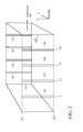
- FIG. 2 is a simplified conceptual diagram illustrating one embodiment of a uniaxial magnet configured to provide a partially enclosed field space
- FIG. 3 is a simplified conceptual diagram illustrating one embodiment of a uni-axial magnet configured to provide a fully enclosed field space.
- FIGS. 2 and 3 illustrate a uni-axial field space defined by substantially planar longitudinal boundaries, i.e ., two opposed longitudinal pole faces 110 and 120, each of which may be oriented substantially normal to the longitudinal axis.
- longitudinal pole faces 110 and 120 do not define substantially planar boundary surfaces.
- Lateral boundaries of the field space may be defined by surfaces aligned parallel to the longitudinal axis. These boundary surfaces are generally coincident with a plurality of lateral pole faces 130, each respective one of which may have a profile in a respective plane that is normal to the longitudinal axis; this respective plane also marks the longitudinal position (denoted x1, x2, ... x4 in FIG. 2 ) of the respective lateral pole face.
- each respective lateral pole face 130 may be shaped with a given profile; in this context, the term "profile" generally refers to the line of intersection between a lateral pole face 130 and the plane marking its longitudinal position.
- the profiles for all respective lateral pole faces 130 generally circumscribe the lateral cross-section of the field space. In accordance with some embodiments, these profiles may be selected to align with a contour associated with the boundary surfaces defined by longitudinal pole faces 110 and 120.
- a "contour” generally refers to a two dimensional (in the y and z dimensions) shape of longitudinal pole faces, which are oriented substantially normal to the longitudinal axis.
- FIG. 2 shows a field space that is only partially enclosed.
- longitudinal boundaries may be defined by longitudinal pole faces 110 and 120, and lateral boundaries may be defined by two series of lateral pole faces 130.
- lateral pole faces 130 are illustrated as having a straight profile, though this is not a requirement.
- the FIG. 2 embodiment generally defines a rectangular enclosure in the x-y plane, leaving the field unconfined in the z dimension. Based upon the dimensions of pole faces 110, 120, and 130, the extent of the generated field in the z dimension may be designated as h.
- a field cage i.e ., a field fence that fully encloses the field space.
- One way to accomplish this is to employ lateral boundary surfaces that have the profile of a closed loop.
- one such embodiment may employ lateral pole faces 130 having a rectangular profile.
- the shape a the profile for lateral pole faces 130 may be arbitrary, and is generally a matter of design choice.
- Various profile shapes for lateral pole faces 130 may be readily adopted to suit the use of the field space, and hence may be application specific.
- FIG. 4 is a simplified diagram illustrating components of one embodiment of an apparatus for producing a uniform magnetic field within a fully enclosed field space as depicted in FIG. 3 .
- FIG. 4 depicts one design of a drive system 400 that may facilitate supplying controlled potentials to pole faces 110, 120, and 130.
- a magnetic field is generated between longitudinal pole faces 110 and 120 of magnetic pole pieces 111 and 121, respectively.
- lateral confinement may be provided by an arbitrary number, n, of lateral pole faces 130 of magnetic pole pieces 131 (only two lateral pole pieces 131 are illustrated in FIG. 4 for clarity).
- the pole faces of pole pieces are, physically, the end of a magnetic conduit; in the FIG. 4 embodiment the end of this conduit is a surface (pole faces 110, 120, and 130) that is contiguous with the boundary surface of the field space.
- the conduits leading to the pole faces are conventionally referred to as pole pieces (111, 121, and 131).
- the term "field frame" generally refers to a pole piece 131 of a closed-loop lateral pole face 130.
- pole pieces 111, 121, and 131 are disposed outside of the field space, with their respective pole faces 110, 120, and 130 generally defining the boundary surfaces of the field space.
- a plurality of lateral pole pieces 131 are disposed at respective lateral boundary planes spaced along the longitudinal axis intermediate longitudinal pole pieces 111 and 121.
- the profiles of lateral pole faces 130 generally define a lateral boundary surface parallel to the longitudinal axis.
- drive system 400 generally comprises a magnetic yoke 410, a plurality of yoke extensions 420 coupling pole pieces 111, 121, and 131 to yoke 410, and a plurality of drive coils 430 comprising coil windings wound around yoke 410 between adjacent extensions 420.
- Yoke 410, extensions 420, and pole pieces 111, 121, and 131 represent magnetic conduits operative to supply controlled magnetostatic potentials to pole faces 110, 120, and 130.
- yoke 410 may provide (in cooperation with extensions 420) a low reluctance magnetic connection between pole pieces 111, 121, and 131.
- Factors influencing the magnitude of a respective magnetostatic potential to a respective pole face 110, 120, or 130 include, but are not limited to, the number of windings in drive coils 430 and the instantaneous or average current passing through drive coils; further, magnetostatic potentials may be affected by the material employed to construct the various components, or by a combination of the foregoing and other factors.
- one longitudinal pole piece 111 is magnetically coupled (via an extension 420) to one end of yoke 410, while another longitudinal pole piece 121 is magnetically coupled (also via an extension 420) to the other end of yoke 410; lateral pole pieces 131 are magnetically couple to yoke 410 intermediate the ends via a respective extension 420.
- yoke 410, extensions 420, and pole pieces 111, 121, and 131 are constructed of or comprise a soft magnetic material and are dimensioned in accordance with a magnetic permeability value and a saturation magnetization value associated with the soft magnetic material. This structural arrangement may facilitate providing a low reluctance magnetic connection between the elements.
- drive system 400 provides a plurality of magnetomotive force generators comprising drive coils 430, each of which is coupled to yoke 410 and disposed between longitudinally adjacent pole pieces 111, 112, and 113.
- FIG. 4 embodiment employs a drive coil 430 wound around yoke 410 between each pair of adjacent extensions 420.
- Each drive coil 430 is a coil winding of current carrying conductor wound around yoke 410.
- the length of extensions 420, as well as the distance between them may determine or influence the available winding space for each drive coil 430.
- a drive current passing through each drive coil 430 produces a magnetomotive force [F] that equals the difference in potential between longitudinally adjacent extensions 420.
- drive coils 430 may be electrically connected in series, although this is not necessary, and may not be desirable in certain applications.
- FIG. 5 is a simplified schematic representation illustrating one example of a design protocol for a confined field uni-axial magnet employing a single yoke. It is noted that FIG. 5 is a longitudinal cross section of the apparatus illustrated in FIG. 4 .
- drive system 400 generally comprises yoke 410 carrying drive coils 431-436 disposed between yoke extensions 420.
- the field space is defined by longitudinal pole faces 110 and 120 (labeled L a and L b in FIG. 5 ), and lateral (or transverse) pole faces 130 (labeled T 1 , T 2 ... T 5 in FIG. 5 ).
- the respective potentials on longitudinal pole faces 110 and 120 will be denoted P(L a ) and P(L b ), whereas on lateral pole faces 130, the respective potentials will be denoted P(T 1 ) . .. P(T 5 ).
- the longitudinal distance between each pair of longitudinally adjacent pole faces is given as s1, s2 ... s6.
- the i th field frame, T i has a potential P(T i ) and is separated from L a by a distance sa i and from L b by a distance sb i .
- magnetomotive force generators may be employed to provide respective magnetostatic potentials to respective poles faces (110, 120, and 130) of longitudinally adjacent pole pieces (111, 121, and 131) in accordance with positions of the pole faces (110, 120, and 130) along the longitudinal axis.
- magnetomotive force generators comprising drive coils 430 may be configured and operative to produce a magnetomotive force having a value that is proportional to a distance between respective longitudinally adjacent pole faces.
- a uni-axial confined field magnet comprising (n-2) field frames (i.e ., lateral pole pieces 131) generally requires (n-1) drive coils 430 to produce (n) P values for (n) pole faces (both longitudinal and lateral).
- the difference in potential between longitudinal pole faces 110 and 120 equals the sum of the magnetic forces produced by drive coils 430.
- the confined field magnet apparatus illustrated in FIGS. 4 and 5 has no additional coil windings as compared to traditional approaches; the embodiments simply employs a segmented coil instead of the single one.
- FIG. 6 is a simplified schematic representation illustrating one example of a design protocol for a confined field uni-axial magnet employing parallel drive systems.
- the schematic shown in FIG. 6 represents one design variation as compared to that described above with reference to FIG. 5 .
- Each drive system 400A and 400B generally operates substantially as described above. However, the arrangement in FIG. 6 tends to improve the uniformity of potential over pole faces 101, 120, and 130.
- Dual drive embodiments may arrange drive systems 400A and 400B symmetrically about the longitudinal axis.
- all pole faces 110, 120, and 130 may be spaced equally (i.e ., the longitudinal distance between adjacent pole faces, whether longitudinal or lateral, is constant) such that the magnetostatic potential increases in equal increments; if identical coil windings are used, they may be connected serially as depicted in FIG. 6 .
- Such a dual drive embodiment of a uni-axial magnet may be employed to provide one field component of a bi-axial magnet as set forth in detail below.
- a drive system such as illustrated in FIGS. 5 and 6 may further comprise a drive circuit (such as a microcontroller, a programmable logic controller (PLC), or an application specific integrated circuit (ASIC), for example).
- a drive circuit such as a microcontroller, a programmable logic controller (PLC), or an application specific integrated circuit (ASIC), for example.
- PLC programmable logic controller
- ASIC application specific integrated circuit
- Such drive logic or circuitry may be employed to control the activation current provided to the drive coils associated with a plurality of magnetomotive force generators; in some implementations, such control may be dictated or influenced as a function of the respective dimensions and magnetic permeability values or other characteristics of each of the pole pieces.
- Bi-axial magnets which enable control of field magnitude and direction, generally may be implemented using two orthogonally aligned uni-axial magnets configured to generate two independently controllable field-components, Hx and Hy.
- the resulting field, H Hx x ⁇ + Hy ⁇ , is the vectorial addition of these field components, where x and y are respective longitudinal axes of each independent uni-axial system.
- orthogonal intersection of the field lanes may be the perfect bi-axial field space.
- each uni-axial field lane is defined by a pair of field fences (i.e ., lateral pole faces) along the system's longitudinal axis
- the orthogonal intersection of these lanes generally defines a rectangular bi-axial field space enclosed by four fence segments as is depicted in FIG.7 . Extending from that field space, each respective lane is terminated by the respective system's longitudinal pole faces.
- each of the four enclosing boundary surfaces serves simultaneously as a lateral boundary for one uni-axial system and as a longitudinal boundary for the other uni-axial system.
- This arrangement facilitates efficiently confining the bi-axial field space.
- a drive system may supply each pole face with a magnetostatic potential having a value that is generally in accord with the uni-axial design protocol set forth above. Efficient driving may be achieved by orthogonally superposing two of the uni-axial drive systems illustrated in Fig. 6 as set forth in more detail below.
- FIG. 8 One embodiment of drive system construction is shown in FIG. 8 . As illustrated in FIG.
- orthogonal superposing of two uni-axial systems has been made possible by segmenting the (formerly solid) longitudinal pole faces into a plurality of (magnetically parallel) separate pole faces to allow for the insertion of drive coils between associated yoke extensions.
- FIG. 7 is a simplified diagram illustrating a collection of pole faces aligned with a rectangular field space of a bi-axial magnet system
- FIG. 8 is a simplified schematic representation illustrating one example of a design protocol for a confined field bi-axial magnet. Comparing FIGS. 6 and 8 , it is apparent that solid longitudinal pole faces 110 and 120 in FIG. 6 have been segmented into a respective plurality of pole faces 110 and 120 in FIG. 8 .
- pole faces 190 may be added to the corners where yokes 410A-410D intersect, although in other embodiments, pole faces 190 may be omitted to simplify construction.
- the parallel drive systems 400A and 400B may be deployed to control the magnetostatic potentials generating and confining the field component Hx, while the drive systems 400C and 400D may be deployed to control the magnetostatic potentials generating and confining the field component Hy.
- pole faces 110 and 120 are longitudinal pole faces and pole faces 130 are lateral or transverse pole faces
- pole faces 130 are longitudinal pole faces and pole faces 110 and 120 are lateral pole faces
- pole faces 190 may provide both lateral and longitudinal confinement, depending upon which of the component fields is considered.
- the Hy drive systems 400C and 400D in parallel produces magnetostatic potentials Py1 to Py7 for generating and confining the Hy field.
- the pole faces 130 (longitudinal pole faces when considering the Hy field component), connected through the magnetic conduit 410B, are all at the potential Py1 while the pole faces 130, connected through the magnetic conduit 410A, are all at the potential Py7.
- Consecutively increasing potentials may be supplied to the pole faces 110 and 120 for confining the Hy field component.
- the magnetostatic potential supplied to each pole piece has a value equal to the sum of values supplied by each drive system for generating the given magnitudes of the Hx and Hy field components.
- the bi-axial assembly of FIG. 8 produces a field that is a vectorial addition of two orthogonal field components, Hx and Hy, each of which is produced by a respective uni-axial system.
- the drive systems 400A-400D work in combination on a rectangular yoke, represented by yokes 410A-410D.
- the collection of all pole faces defines a rectangular enclosure where there exists a laterally confined Hx field and a laterally confined Hy field.
- the combined field, H Hx x ⁇ + Hy ⁇ , is the vectorial addition of these field components, where x and y are respective longitudinal axes of each independent uni-axial system.
- the magnitude and direction of the combined field may be controlled by controlling the magnitude of Hx and Hy individually.
- the enclosure of this region generally comprises a pair of field fences parallel to the x axis (i.e., pole faces 130 and 190) and a pair of field fences parallel to the y axis ( i.e ., pole faces 110, 120, and 190).
- the FIG. 8 embodiment seven pole faces are employed for each "fence," with pole faces 190 being common to adjacent fences. It is noted that the number of pole faces is an arbitrary design choice, and that more or fewer may be employed in accordance with overall system requirements, manufacturing considerations, cost constraints, or a combination of these and other factors.
- each pole piece (111, 121, 131, and 191) may be connected to a yoke (410A-410D) via a yoke extension 420, providing a low reluctance magnetic connection to supply pole faces 110, 120, 130, and 190 with a desired magnetostatic potential.
- a yoke (410A-410D)
- a yoke extension 420 providing a low reluctance magnetic connection to supply pole faces 110, 120, 130, and 190 with a desired magnetostatic potential.
- six drive coils (Cx1-Cx6 and Cy1-Cy6) on each yoke 410A-410D may be operative to generate respective magnetomotive forces (e.g., Fx1, Fx2, ... Fx6 along the x axis, and Fy1, Fy2 ... Fy6 along the y-axis) as desired.
- drive currents Ix and Iy may be employed to produce potentials labeled Px1, Px2 ... Px7 along the x axis, and Py1, Py2 ... Py7 along the y axis.
- FIG. 8 depicts a regular rectilinear and orthogonal pattern of equipotential lines connecting corresponding pole faces on opposite sides of the respective longitudinal axes. This suggests perfect uniformity of each field component, Hx and Hy, and hence of the combined bi-axial field. Ignoring perturbations along the boundaries as discussed above, perfect uniformity would indeed exist if the field space extended without limit along the z axis. Given that the spatial extent of the bi-axial field space is limited, as set forth in more detail below, a distortion of field uniformity possibly exists near or beyond the geometrical floor or ceiling of the field space.
- pole faces 110,190 along the left of FIG. 8 ⁇ i.e., the left "y-fence" are at the same potential (Px1)
- pole faces 120,190 along the right y-fence are at the same potential (Px7)
- Pole faces 130 along both x-fences carry a respective potential (Px2 ... Px6) determined as a function of location along the x axis.
- pole faces 130,190 along the top x-fence are at the same potential (Py1), while pole faces 130,190 along the bottom x-fence are at the same potential (Py7).
- Pole faces 110 and 120 along the y-fences carry a respective potential (Py2 ... Py6) determined as a function of location along the y axis. With all drive systems 400A-400D activated, the potential at each pole face 110,120,130, and 190 may be equal to the sum of values generated by each uni-axial system individually.
- a biaxial magnet may employ a square region of confinement provided by field fences having pole faces at equal spacing.
- the magnetomotive forces to be generated are hence all equal, and each drive system may employ identical coils; each coil in a respective drive system may be connected in series and activated with the same drive current.
- Other configurations are also possible, as will be understood by those of skill in the art, and the present disclosure is not intended to be limited by any particular shape, geometric arrangement, or density of pole faces defining the boundary surfaces of the field space.
- the embodiment illustrated as a simplified diagram in FIG. 8 encloses a bi-axial field space in the x-y plane, but the field may generally be unconfined along the z-axis.
- the required gap implies that there exists some opening in the enclosure.
- the enclosure depicted schematically in FIG. 7 exemplifies a simple enclosure geometry providing partial confinement of a bi-axial field space.
- a rectangular enclosure employs a field fence with sixteen total pole faces: five along each side, including four shared corner pole faces.
- each pole face has a uniform height, h.
- the floor and ceiling designations are merely geometrical as the generated magnetic field will tend to bulge through these planes.
- the field space may be confined more fully, for example, by bending or curving the ends of the pole faces inward (i.e., towards each other, generating a concave profile), and thereby improve field uniformity inside the enclosure.
- it may be desirable in some instances to broaden that region for example, by curving the ends of the pole faces outward ( i.e., away from each other, generating a convex profile).
- FIGS. 9A-9C are simplified diagrams illustrating various embodiments of pole face profiles
- FIGS. 10A-10C are simplified diagrams illustrating an arrangement of pole faces in one embodiment of a bi-axial magnet employing pole faces having convex profiles.
- Some representative profiles worth considering for various applications are straight ( FIG. 9A ), concave ( FIG. 9B ), and convex ( FIG. 9C).
- FIG. 9 also indicates a resulting field configuration associated with each respective profile shape. The field configurations may be deduced by knowing that along a given pole face, the field vector is locally perpendicular to the profile. Implementation of non-straight profiles, however, creates challenges that do not arise with a uni-axial system in which the profile defines the shape of the lateral boundary surface only.
- each pole face in a bi-axial system is used concurrently as a longitudinal boundary component by one system and as a lateral boundary component by the other system.
- FIGS. 10A and 10B show, respectively, intersection points of pole faces having convex profiles for a plane at a first elevation [z1] and a plane at a second elevation [z2].
- FIG. 10C depicts, at progressively lower elevations, the track of intersection points if congruency is to be retained over that range of elevation. As demonstrated by the plots in FIG. 10C , it may be desirable in some instances that each profile lie in an azimuthal plane.
- the profile for each pole face may be scaled in accordance with azimuth.
- it may be desirable that the profiles of the pole faces are shaped and oriented such that the profiles' positions change congruently as a function of elevation.
- conduits e.g., yoke 410, extensions 420, and pole pieces 111, 121, 131, and 191 transmit magnetostatic potentials without loss along the conduit.
- soft magnetic materials i.e., generally characterized by a large value of permeability and a lack of hysteresis.
- Some implementations may benefit from linearity of response; accordingly, it may be desirable to minimize or eliminate saturation effects. It will be appreciated that some applications, therefore, may require that the various conduits have sufficient cross-section for a given material with a given value of saturation magnetization.
- a drive system comprising a drive circuit or logic (such as may be embodied in a microcontroller, a PLC, or an ASIC).
- drive logic or circuitry may be employed to control the activation current provided to the drive coils associated with a plurality of magnetomotive force generators.
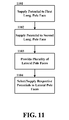
- FIG. 11 is a simplified flow diagram illustrating general operation of one embodiment of a method of producing a substantially uniform magnetic field having a controllable magnitude.
- a magnetostatic potential may be supplied to a first longitudinal pole face at a first longitudinal boundary oriented substantially normal to a longitudinal axis as indicated at block 1101.
- a magnetostatic potential may be supplied to a second longitudinal pole face at a second longitudinal boundary oriented substantially normal to the longitudinal axis as indicated at block 1102.
- a plurality of lateral pole faces may be provided as indicated at block 1103.
- the lateral pole faces may generally be disposed along a lateral boundary surface intermediate the first and second longitudinal boundaries, and each lateral pole face may be disposed in a respective lateral boundary plane oriented substantially normal to the longitudinal axis.
- a respective magnetostatic potential may be supplied to each respective one of the lateral pole faces as indicated at block 1104.
- the value of the respective magnetostatic potential may be selected in accordance with a position of the respective lateral boundary plane relative to the first and second longitudinal boundaries.
- FIG. 12 is a simplified flow diagram illustrating general operation of one embodiment of a method of producing a substantially uniform magnetic field having a controllable magnitude and direction.
- a method may begin by defining two orthogonal field components (block 1201): a first field component to be generated along a first longitudinal axis; and a second field component to be generated along a second longitudinal axis.
- a plurality of pole faces may be positioned at locations along each of the first and second longitudinal axes as indicated at block 1202.
- a first magnetostatic potential to apply to a first plurality of longitudinal pole faces at a first longitudinal boundary may be selected (as indicated at block 1203), while a second magnetostatic potential to apply to a second plurality of longitudinal pole faces at a second longitudinal boundary may be selected (as indicated at block 1204).
- a plurality of lateral pole faces may be identified as indicated at block 1205. As set forth above, these lateral pole faces may be disposed along a lateral boundary surface intermediate the first and second longitudinal boundaries, and each may be disposed in a respective lateral boundary plane oriented substantially normal to the longitudinal axis. For each respective one of the plurality of lateral pole faces, a value of a respective magnetostatic potential may be selected in accordance with a position of the respective lateral boundary plane relative to the first and second longitudinal boundaries (block 1206).
- the operations depicted at blocks 1203 through 1206 may be repeated for each of the orthogonal field components, as indicated by the loop back to decision block 1299. If a determination is made that both field components have not been selected, the process may continue, iterating the operations at blocks 1203-1206 for the second field component. If, on the other hand, a determination is made that both field components have been selected, the magnetic field may be generated by vectorial addition of the field components. In particular, selected values of magnetostatic potential may be supplied to all pole faces as indicated at block 1210. As noted above, the respective potential to be supplied to each respective pole face may be an addition of the potentials determined for that pole face in each of the uni-axial systems. In the foregoing manner, a substantially uniform magnetic field that is controllable in magnitude and direction within the field space may be generated.
- FIG. 12 may have particular utility when used in conjunction with a closed loop management or control system.
- one or more field sensors e.g., at least one field sensor for each field component
- feedback may be employed dynamically (e.g., by drive circuitry or logic as set forth above) to alter or otherwise to adjust the magnetostatic potentials selected for various of the pole faces in the system.
- This closed loop feedback is represented in FIG. 12 by the dashed arrow from block 1206 back to block 1203.
- FIG. 13 is a simplified flow diagram illustrating general operation of another embodiment of a method of producing a substantially uniform magnetic field having a controllable magnitude and direction.
- a method may begin by defining a field plane having two orthogonal axes (block 1301), each generally defining a longitudinal axis for a respective field component.
- the spatial boundary of the field to be generated may be defined as indicated at block 1302; in some implementations, the boundary may be designated or determined by identifying a rectangular region in the field plane bounded by boundary surfaces intersecting the field plane perpendicular to each longitudinal axis. These boundary surfaces, or enclosing surfaces, serve to enclose the field within a particular space; as noted above, it is not possible fully to enclose a bi-axial field space, but the field space may readily be enclosed in the field plane defined by the orthogonal longitudinal axes.
- a spatial boundary in the field plane may generally comprise a respective pair of boundary surfaces aligned parallel to, and positioned on opposite sides of, each respective longitudinal axis.
- a plurality of pole faces may be positioned at each of the boundary surfaces (block 1303) to facilitate definition of the spatial boundaries of the field space.
- a longitudinal boundary surface for one field component may be a lateral boundary surface for the other field component (e.g., Hy) and vice-versa.
- the pole faces at the boundary surfaces that are perpendicular to the respective longitudinal axis may be designated as longitudinal pole faces, and the pole faces at the boundary surfaces that are parallel to the respective longitudinal axis may be designated as lateral pole faces.
- a method may designate as "longitudinal” the two boundary surfaces (and the pole faces at those boundary surfaces) oriented perpendicular to a particular longitudinal axis, and may then designate as "lateral” the two boundary surfaces (and the pole faces at those boundary surfaces) oriented parallel to that particular longitudinal axis; the inverse would be true for the second field component.
- each respective field component may be determined as indicated at block 1305. As set forth above, these magnitudes may be selected or otherwise determined such that a vectorial addition of the two field components yields a desired magnitude and direction of the magnetic field to be produced. Each field component may be produced and confined as indicated at block 1306. With respect to production, a method may produce each respective field component by selecting a first value of magnetostatic potential to all the pole faces disposed along its first longitudinal boundary surface and selecting a second value of magnetostatic potential to all the pole faces disposed along its second longitudinal boundary surface. As noted above, the difference between these magnetostatic potentials may be proportional to the determined or desired magnitude of the respective field component.
- a method may confine each respective field component by selecting, for each pole face disposed along a lateral boundary, a magnetostatic potential having a value intermediate the values supplied to the pole faces at the longitudinal boundaries.
- a respective value for a lateral pole face may be proportional to the distances of separation between that lateral pole face and each longitudinal boundary.
- selecting or otherwise determining values of magnetostatic potentials to be supplied to the pole faces may generally comprise selecting magnetostatic potentials that are proportional to the selected magnitudes of each of the first and second field components.
- a magnetic field to be generated is the vectorial combination of each field component.
- a method may supply, to each pole face, a magnetostatic potential having a value equal to the sum of values associated with producing and confining each of the two field components. This is indicated at block 1307.
- the operation depicted at block 1307 may supply magnetostatic potentials to the collection of pole faces using a shared magnetic conduit that is an orthogonal superposition of respective uni-axial drive systems.
- FIG. 13 does not necessarily imply a particular order or sequence of events, nor is it intended to exclude other possibilities.
- the operation depicted at block 1305 may precede the operations at any other block, and the operations at blocks 1302 and 1303 or 1303 and 1304 may occur substantially simultaneously with each other. Other sequences or combinations of the operations are contemplated.
Landscapes
- Physics & Mathematics (AREA)
- Electromagnetism (AREA)
- Engineering & Computer Science (AREA)
- Power Engineering (AREA)
- Condensed Matter Physics & Semiconductors (AREA)
- General Physics & Mathematics (AREA)
- Magnetic Resonance Imaging Apparatus (AREA)
- Measuring Magnetic Variables (AREA)
- Linear Motors (AREA)
Applications Claiming Priority (2)
| Application Number | Priority Date | Filing Date | Title |
|---|---|---|---|
| US12/128,474 US8179220B2 (en) | 2008-05-28 | 2008-05-28 | Confined field magnet system and method |
| EP09755739.1A EP2286421B1 (en) | 2008-05-28 | 2009-05-28 | Confined field magnet system and method |
Related Parent Applications (1)
| Application Number | Title | Priority Date | Filing Date |
|---|---|---|---|
| EP09755739.1 Division | 2009-05-28 |
Publications (1)
| Publication Number | Publication Date |
|---|---|
| EP2620957A1 true EP2620957A1 (en) | 2013-07-31 |
Family
ID=40886109
Family Applications (2)
| Application Number | Title | Priority Date | Filing Date |
|---|---|---|---|
| EP13162604.6A Withdrawn EP2620957A1 (en) | 2008-05-28 | 2009-05-28 | Confined field magnet system and method |
| EP09755739.1A Not-in-force EP2286421B1 (en) | 2008-05-28 | 2009-05-28 | Confined field magnet system and method |
Family Applications After (1)
| Application Number | Title | Priority Date | Filing Date |
|---|---|---|---|
| EP09755739.1A Not-in-force EP2286421B1 (en) | 2008-05-28 | 2009-05-28 | Confined field magnet system and method |
Country Status (4)
| Country | Link |
|---|---|
| US (2) | US8179220B2 (https=) |
| EP (2) | EP2620957A1 (https=) |
| JP (1) | JP5511800B2 (https=) |
| WO (1) | WO2009146378A1 (https=) |
Families Citing this family (1)
| Publication number | Priority date | Publication date | Assignee | Title |
|---|---|---|---|---|
| DE112020000394T5 (de) * | 2019-01-11 | 2021-09-23 | Kanazawa Institute Of Technology | Magnetfeld-kalibrierungsvorrichtung und verfahren zur kalibrierung einer magnetismus-messvorrichtung mit dieser vorrichtung |
Citations (3)
| Publication number | Priority date | Publication date | Assignee | Title |
|---|---|---|---|---|
| WO1988006798A1 (fr) * | 1987-03-03 | 1988-09-07 | Commissariat A L'energie Atomique | Systeme d'aimants permanents pour un champ magnetique intense |
| DE19742548A1 (de) * | 1997-09-26 | 1999-04-08 | Otten Ernst Wilhelm Prof Dr | Transporteinrichtung für kernspinpolarisierte Gase, insbesondere Edelgase, wie die Isotope ·3·He, ·1··2··9·Xe |
| US7199689B1 (en) * | 2006-01-09 | 2007-04-03 | Brk Wireless Company, Inc | High field NMR permanent magnetic structure |
Family Cites Families (14)
| Publication number | Priority date | Publication date | Assignee | Title |
|---|---|---|---|---|
| NL133615C (https=) * | 1962-10-04 | |||
| FR2562785B1 (fr) | 1984-04-13 | 1988-04-15 | Commissariat Energie Atomique | Systeme a aimants permanents destine a l'imagerie par resonance magnetique nucleaire, notamment pour l'examen du corps humain |
| US4647887A (en) * | 1984-12-24 | 1987-03-03 | The United States Of America As Represented By The Secretary Of The Army | Lightweight cladding for magnetic circuits |
| JPS61175600A (ja) * | 1985-01-31 | 1986-08-07 | 日本電信電話株式会社 | パルス電磁石 |
| US4667174A (en) * | 1985-08-23 | 1987-05-19 | Resonex, Inc. | Magnet assembly for magnetic resonance imaging and method of manufacture |
| FR2605450B1 (fr) * | 1986-10-17 | 1988-12-02 | Thomson Cgr | Aimant permanent cylindrique pour produire un champ d'induction uniforme et transverse |
| JPH01109799A (ja) * | 1987-10-23 | 1989-04-26 | Mitsubishi Electric Corp | 磁気シールド装置 |
| EP0525246A1 (de) * | 1991-08-01 | 1993-02-03 | Siemens Aktiengesellschaft | Magneteinrichtung mit einem ein magnetisches Streufeld erzeugenden Jochkörper |
| US5319339A (en) * | 1993-03-08 | 1994-06-07 | The United States Of America As Represented By The Secretary Of The Army | Tubular structure having transverse magnetic field with gradient |
| US5576679A (en) * | 1994-10-25 | 1996-11-19 | Shin-Etsu Chemical Co., Ltd. | Cylindrical permanent magnet unit suitable for gyrotron |
| WO1999040593A1 (en) * | 1998-02-09 | 1999-08-12 | Odin Medical Technologies Ltd | A method for designing open magnets and open magnetic apparatus for use in mri/mrt probes |
| JP3698099B2 (ja) * | 2001-12-14 | 2005-09-21 | 株式会社日立製作所 | 磁気共鳴撮像装置用マグネット |
| JP2005084022A (ja) * | 2003-09-11 | 2005-03-31 | Neomax Co Ltd | センサ検査用磁場発生装置およびセンサ検査装置 |
| JP2008249619A (ja) * | 2007-03-30 | 2008-10-16 | Tdk Corp | 透磁率測定用プローブ及びそれを用いた透磁率測定装置 |
-
2008
- 2008-05-28 US US12/128,474 patent/US8179220B2/en not_active Expired - Fee Related
-
2009
- 2009-05-28 EP EP13162604.6A patent/EP2620957A1/en not_active Withdrawn
- 2009-05-28 WO PCT/US2009/045507 patent/WO2009146378A1/en not_active Ceased
- 2009-05-28 EP EP09755739.1A patent/EP2286421B1/en not_active Not-in-force
- 2009-05-28 JP JP2011511826A patent/JP5511800B2/ja not_active Expired - Fee Related
-
2012
- 2012-04-27 US US13/458,535 patent/US8294543B2/en not_active Expired - Fee Related
Patent Citations (3)
| Publication number | Priority date | Publication date | Assignee | Title |
|---|---|---|---|---|
| WO1988006798A1 (fr) * | 1987-03-03 | 1988-09-07 | Commissariat A L'energie Atomique | Systeme d'aimants permanents pour un champ magnetique intense |
| DE19742548A1 (de) * | 1997-09-26 | 1999-04-08 | Otten Ernst Wilhelm Prof Dr | Transporteinrichtung für kernspinpolarisierte Gase, insbesondere Edelgase, wie die Isotope ·3·He, ·1··2··9·Xe |
| US7199689B1 (en) * | 2006-01-09 | 2007-04-03 | Brk Wireless Company, Inc | High field NMR permanent magnetic structure |
Also Published As
| Publication number | Publication date |
|---|---|
| EP2286421A1 (en) | 2011-02-23 |
| EP2286421B1 (en) | 2013-05-22 |
| JP5511800B2 (ja) | 2014-06-04 |
| US8294543B2 (en) | 2012-10-23 |
| JP2011522424A (ja) | 2011-07-28 |
| US20090295378A1 (en) | 2009-12-03 |
| WO2009146378A1 (en) | 2009-12-03 |
| US20120212310A1 (en) | 2012-08-23 |
| US8179220B2 (en) | 2012-05-15 |
Similar Documents
| Publication | Publication Date | Title |
|---|---|---|
| US4931760A (en) | Uniform magnetic field generator | |
| US4355236A (en) | Variable strength beam line multipole permanent magnets and methods for their use | |
| CA2913801C (en) | Magnet assemblies | |
| US5332971A (en) | Permanent magnet for nuclear magnetic resonance imaging equipment | |
| TWI449306B (zh) | 線性馬達 | |
| CA1331481C (en) | Periodic permanent magnet structure for use in electronic devices | |
| US8077002B2 (en) | Open MRI magnetic field generator | |
| WO1993018707A1 (fr) | Generateur de champ magnetique destine a l'imagerie par resonance magnetique_____________________________________________________ | |
| CN110857970B (zh) | 磁体组件以及用于制造磁体组件的方法 | |
| EP0192331A1 (en) | Electromagnet | |
| Insinga et al. | Globally optimal segmentation of permanent-magnet systems | |
| Leupold et al. | Applications of yokeless flux confinement | |
| KR0135210B1 (ko) | 자기공명영상장치(mri)용 자기장 발생장치 | |
| EP2286421B1 (en) | Confined field magnet system and method | |
| US5914600A (en) | Planar open solenoidal magnet MRI system | |
| CN106229106B (zh) | 一种奇数层的Halbach阵列永磁体装置的设计与制作方法 | |
| US8543177B2 (en) | Superconducting magnet systems | |
| CN113009394B (zh) | 一种静磁场发生装置 | |
| Shirasawa et al. | Development of multi‐polarization‐mode undulator | |
| CN104849007B (zh) | 磁场跟踪补偿的四磁路对称励磁矩形开放磁场式电磁振动台磁路结构 | |
| CN104848930B (zh) | 涡流补偿的双排永磁体向心励磁矩形开放磁场式电磁振动台磁路结构 | |
| JP2596836B2 (ja) | 磁場発生装置 | |
| US7394255B2 (en) | Single-sided magnetic resonance magnet assembly | |
| RU2620579C2 (ru) | Магнитная система | |
| WO2002052301A1 (en) | High efficiency planar open magnet mri system structure and arranged to provide orthogonal ferrorefractory effect |
Legal Events
| Date | Code | Title | Description |
|---|---|---|---|
| PUAI | Public reference made under article 153(3) epc to a published international application that has entered the european phase |
Free format text: ORIGINAL CODE: 0009012 |
|
| AC | Divisional application: reference to earlier application |
Ref document number: 2286421 Country of ref document: EP Kind code of ref document: P |
|
| AK | Designated contracting states |
Kind code of ref document: A1 Designated state(s): AT BE BG CH CY CZ DE DK EE ES FI FR GB GR HR HU IE IS IT LI LT LU LV MC MK MT NL NO PL PT RO SE SI SK TR |
|
| 17P | Request for examination filed |
Effective date: 20140131 |
|
| RBV | Designated contracting states (corrected) |
Designated state(s): AT BE BG CH CY CZ DE DK EE ES FI FR GB GR HR HU IE IS IT LI LT LU LV MC MK MT NL NO PL PT RO SE SI SK TR |
|
| 17Q | First examination report despatched |
Effective date: 20140620 |
|
| GRAP | Despatch of communication of intention to grant a patent |
Free format text: ORIGINAL CODE: EPIDOSNIGR1 |
|
| INTG | Intention to grant announced |
Effective date: 20160418 |
|
| STAA | Information on the status of an ep patent application or granted ep patent |
Free format text: STATUS: THE APPLICATION IS DEEMED TO BE WITHDRAWN |
|
| 18D | Application deemed to be withdrawn |
Effective date: 20160830 |