EP2278302B1 - Verfahren zur messung von zeitprofilen optischer pulse - Google Patents
Verfahren zur messung von zeitprofilen optischer pulse Download PDFInfo
- Publication number
- EP2278302B1 EP2278302B1 EP10010839.8A EP10010839A EP2278302B1 EP 2278302 B1 EP2278302 B1 EP 2278302B1 EP 10010839 A EP10010839 A EP 10010839A EP 2278302 B1 EP2278302 B1 EP 2278302B1
- Authority
- EP
- European Patent Office
- Prior art keywords
- sample
- pulse
- fourier transform
- composite
- symmetric
- Prior art date
- Legal status (The legal status is an assumption and is not a legal conclusion. Google has not performed a legal analysis and makes no representation as to the accuracy of the status listed.)
- Expired - Lifetime
Links
Images













Classifications
-
- G—PHYSICS
- G01—MEASURING; TESTING
- G01J—MEASUREMENT OF INTENSITY, VELOCITY, SPECTRAL CONTENT, POLARISATION, PHASE OR PULSE CHARACTERISTICS OF INFRARED, VISIBLE OR ULTRAVIOLET LIGHT; COLORIMETRY; RADIATION PYROMETRY
- G01J11/00—Measuring the characteristics of individual optical pulses or of optical pulse trains
-
- G—PHYSICS
- G01—MEASURING; TESTING
- G01N—INVESTIGATING OR ANALYSING MATERIALS BY DETERMINING THEIR CHEMICAL OR PHYSICAL PROPERTIES
- G01N21/00—Investigating or analysing materials by the use of optical means, i.e. using sub-millimetre waves, infrared, visible or ultraviolet light
- G01N21/62—Systems in which the material investigated is excited whereby it emits light or causes a change in wavelength of the incident light
- G01N21/63—Systems in which the material investigated is excited whereby it emits light or causes a change in wavelength of the incident light optically excited
- G01N21/636—Systems in which the material investigated is excited whereby it emits light or causes a change in wavelength of the incident light optically excited using an arrangement of pump beam and probe beam; using the measurement of optical non-linear properties
-
- G—PHYSICS
- G06—COMPUTING OR CALCULATING; COUNTING
- G06F—ELECTRIC DIGITAL DATA PROCESSING
- G06F17/00—Digital computing or data processing equipment or methods, specially adapted for specific functions
- G06F17/10—Complex mathematical operations
- G06F17/14—Fourier, Walsh or analogous domain transformations, e.g. Laplace, Hilbert, Karhunen-Loeve, transforms
- G06F17/141—Discrete Fourier transforms
Definitions
- the present invention relates generally to the field of measuring attributes of a physical system and, more particularly, relates to methods of measuring a non-symmetric physical function.
- Various optical devices are based on induced second-order susceptibilities in silica-based glass waveguides (e.g., electro-optic modulators, switches, parametric amplifiers).
- silica-based glass waveguides e.g., electro-optic modulators, switches, parametric amplifiers.
- G. Bonfrate et al. describe optical parametric oscillators useful for the study of quantum interference and quantum cryptography, and for metrology applications in Parametric Fluorescence in Periodically Poled Silica Fibers, Applied Physics Letters, Vol. 75, No. 16, 1999, pages 2356-2358 .
- Second-order susceptibility can be induced in a several-microns-thick region of fused silica (a material that is not normally centro-symmetric, and therefore normally does not exhibit a second-order susceptibility) by poling at elevated temperatures. This phenomenon has been described by R.A. Myers et al. in Large Second-Order Nonlinearity in Poled Fused Silica, Optics
- FIGs 1A and 1B schematically illustrate the poling of a silica wafer 1.
- poling typically comprises using an anode electrode 2 placed proximate to one surface 3 of the wafer 1 and a cathode electrode 4 placed proximate to the opposite surface 5 of the wafer 1.
- a voltage is applied across the wafer 1 for a period of time, resulting in a second-order optical nonlinearity profile.
- the profile has a thickness and is localized beneath the surface 3 where the anode electrode was placed, as schematically illustrated in Figure 1B .
- anodic surface refers to the surface which is placed proximate to the anode electrode
- cathodic surface refers to the surface which is placed proximate to the cathode electrode
- the field of poled silica has suffered from the lack of a common method to reliably measure the second-order optical nonlinearity profile of poled samples. This absence of a reliable procedure for measuring nonlinearity profiles may be the reason, at least in part, for wide discrepancies in the measured magnitudes and the positions of the nonlinearity profiles of various poled systems as reported in the literature.
- the Maker fringe (MF) technique is the most common method currently used to investigate the nonlinearity profile of poled silica.
- the MF technique comprises focusing a pulsed laser beam of intensity I 1 (known as the fundamental signal) onto a sample at an incident angle ⁇ and measuring the intensity I 2 of the second harmonic (SH) signal generated within the nonlinear region as a function of the incident angle ⁇ .
- f ( ⁇ , n 1 , n 2 ) accounts for both the power loss due to reflection suffered by the fundamental and the SH beams, and the projection of the input electric field along the appropriate direction.
- f ( ⁇ , n 1 , n 2 ) depends on both the polarization of the input fundamental wave and the geometry of the second harmonic generation configuration.
- the exact formula of f ( ⁇ , n 1 , n 2 ) is given by D. Pureur, et al. in Absolute Measurement of the Second-Order Nonlinearity Profile in Poled Silica, Optics Letters, Vol. 23, 1998, pages 588-590 , which is incorporated in its entirety by reference herein. This phenomenon is also described by P.D. Maker et al. in Effects of Dispersion and Focusing on the Production of Optical Harmonics, Physics Review Letters, Vol. 8, No. 1, 1962, pages 21-22 .
- the conversion efficiency ⁇ TM ( ⁇ ) is obtained experimentally by rotating the sample with respect to the incident laser beam and measuring the power of the SH signal as a function of the incident angle ⁇ . Due to dispersion of the laser beam, ⁇ k is finite and ⁇ TM ( ⁇ ) exhibits oscillations (called the Maker fringes) which pass through several maxima and minima. The objective of this measurement is to retrieve the second-order nonlinearity profile d 33 ( z ). The absolute value of the integral in Equation 1 is the amplitude of the Fourier transform of d 33 ( z ).
- US4792230 discloses a method and apparatus for measuring ultrashort optical pulses.
- the invention is defined by the method of claim 1.
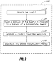
- Figure 2 is a flow diagram of a method 100 of measuring a second-order optical nonlinearity profile of a sample 10 of Figure 1B .
- references to figures 1-20 and 22-39 are merely intended as examples outside the scope of the invention.
- the sample 10 is provided in an operational block 110.
- the sample 10 has the second-order optical nonlinearity profile 15 to be measured.
- a surface of the sample 10 is placed proximate to a surface of a supplemental sample 20, as schematically illustrated in Figures 3A-3C and 4A-4D .
- the sample 10 and supplemental sample 20 form a first composite sample 30 having an odd second-order optical nonlinearity profile 35.
- a Fourier transform magnitude of the odd second-order optical nonlinearity profile 35 of the composite sample 30 is measured.
- the sample nonlinearity profile is calculated using the Fourier transform magnitude of the first composite nonlinearity profile.
- calculating the sample nonlinearity profile comprises using the measured Fourier transform magnitude to determine a Fourier transform of the odd second-order optical nonlinearity profile 35 of the composite sample 30, and calculating an inverse Fourier transform of the determined Fourier transform.
- the calculated inverse Fourier transform provides information regarding the second-order optical nonlinearity profile 15 of the sample 10.
- the information comprises the magnitude and sign of the second-order optical nonlinearity profile 15 as a function of depth below the surface of the sample 10.
- the information comprises the position of the second-order optical nonlinearity profile 15 below the surface of the sample 10.
- the second-order optical nonlinearity profile 15 of the sample 10 is non-symmetric, while in other embodiments, the second-order optical nonlinearity profile 15 of the sample 10 is symmetric about the origin (e.g., odd function of z).
- Other existing methods are useful for measuring second-order optical nonlinearity profiles which are symmetric about the origin, but such existing methods are not compatible with non-symmetric profiles.
- Embodiments described herein are compatible with both symmetric and non-symmetric second-order optical nonlinearity profiles. Since it is not generally known whether the second-order optical nonlinearity profile is non-symmetric or symmetric about the origin prior to measurement, embodiments described herein provide a general method of measurement independent of the symmetry about the origin of the profile to be determined.
- the information comprises whether the second-order optical nonlinearity profile is symmetric or non-symmetric about the origin.
- Embodiments of the present invention can be used to determine the nonlinearity profile of any optically nonlinear material (e.g., crystalline, amorphous, organic, or inorganic) in a bulk form or in a film form.
- the nonlinear material comprises an organic material, such as polymers and solids doped with dye molecules.
- the nonlinear material comprises inorganic materials such as crystalline lithium niobate or amorphous materials (e.g., oxide-based, fluoride-based, or sulfide-based glasses).
- the sample 10 comprises silica glass that has been poled so as to induce a second-order optical nonlinearity profile in the sample 10.
- a fused silica wafer comprised of INFRASIL quartz glass and measuring 1" x 1" x 0.1" (i.e., 2.54 cm x 2.54 cm x 2.54 mm) can be poled at approximately 270°C in air by using an anode electrode placed proximate to one surface of the wafer (i.e., the anodic surface) and a cathode electrode placed proximate to the opposite surface of the wafer (i.e., the cathodic surface) to apply approximately 5 kV across the wafer for approximately 15 minutes.
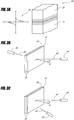
- FIGS 3B and 3C schematically illustrate two measurement configurations in accordance with embodiments of the present invention.
- the composite sample 30 has a surface normal direction n .
- a laser 40 produces a laser beam 42 of light with a fundamental frequency v .
- the laser beam 42 is incident on the composite sample 30 at an angle ⁇ relative to the surface normal direction n .
- a detector 50 is positioned on the opposite side of the composite sample 30 so as to detect the second harmonic (SH) signal 52 (having a frequency 2v) from the composite sample 30.
- SH second harmonic
- appropriate optical filters are placed between the composite sample 30 and the detector 50 to reduce the laser power transmitted by the composite sample 30 to be well below the weaker power level of the SH signal.
- the embodiment of Figure 3B can be considered to be a transmission configuration.
- the detector 50 is positioned on the same side of the composite sample 30 as the laser 40 so as to detect the SH signal 52.
- the embodiment of Figure 3C can be considered to be a reflection configuration.
- double pass refers to configurations in which Maker fringe data are obtained from two wafers proximate to one another (e.g., as shown in Figures 3B and 3C ).
- single pass refers to configurations in which Maker fringe data are obtained from a single wafer.
- the composite sample 30 is positioned so that the laser beam 42 is first incident on the sample 10, while in other embodiments, the laser beam 42 is first incident on the supplemental sample 20.
- the SH signal 52 is measured as a function of the incident angle ⁇ of the laser beam 42 by rotating the composite sample 30 relative to the laser beam 42.
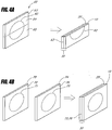
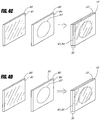
- Figures 4A-4D schematically illustrate various embodiments of the supplemental sample 20 in accordance with embodiments of the present invention.
- the supplemental sample 20 has a second-order optical nonlinearity profile substantially identical to that of the sample 10.
- the sample 10 and the supplemental sample 20 comprise two portions of a common sample 60.
- a fused silica wafer which serves as the common sample 60 can be poled as described above, resulting in a poled region 62 beneath the anodic surface 63 of the wafer 60.
- the wafer can then be cut in half, producing two portions 64, 65, which can serve as the sample 10 and the supplemental sample 20.
- the sample 10 and the supplemental sample 20 can then be placed proximate to one another, thereby forming the composite sample 30.
- the second-order optical nonlinearity profile of the supplemental sample 20 is effectively multiplied by -1.
- the physical reason for this sign change is that during poling, the symmetry of the intrinsic material is broken along the z direction.
- the second-order optical nonlinearity profile of the composite sample 30 is an odd function.
- the sample 10 and the supplemental sample 20 are placed proximate to one another with the poled regions of the portions 64, 65 proximate to one another (referred to herein as an anode-to-anode configuration).
- the two halves of the surface 63 are in contact with one another, while in other embodiments, there is empty space or a spacer material between the two portions 64, 65.
- This spacer material can comprise an index-matching gel which reduces total internal reflection.
- the sample 10 and the supplemental sample 20 are placed proximate to one another with the poled regions of the portions 64, 65 on the outer sides of the composite sample 30 (referred to herein as a cathode-to-cathode configuration).
- the two portions 64, 65 are in contact with one another, while in other embodiments, there is empty space or a spacer material (e.g., index-matching gel) between the two portions 64, 65.
- the supplemental sample 20 is prepared using substantially identical conditions as those used to prepare the sample 10.
- two substantially identical fused silica wafers 70, 74 can be poled sequentially or simultaneously as described above using substantially identical conditions, resulting in corresponding poled regions 71, 75 beneath corresponding surfaces 72, 76.
- one wafer 70 serves as the sample 10
- the other wafer 74 serves as the supplemental sample 20.
- the sample 10 and the supplemental sample 20 can then be placed proximate to one another, thereby forming the composite sample 30.
- the sample 10 and the supplemental sample 20 are placed proximate to one another with the poled regions 71, 75 proximate to one another in the anode-to-anode configuration.
- the two surfaces 72, 76 are in contact with one another, while in other embodiments, there is empty space or a spacer material (e.g., index-matching gel), between the two wafers 70, 74.
- the sample 10 and the supplemental sample 20 are placed proximate to one another with the poled regions 71, 75 on opposite sides of the composite sample 30 in the cathode-to-cathode configuration.
- the two wafers 70, 74 are in contact with one another, while in other embodiments, there is empty space or a spacer material (e.g., index-matching gel) between the two wafers 70, 74.
- the supplemental sample 20 comprises a reflector 80 with a reflecting surface 81.
- the sample 10 of such embodiments can comprise a wafer 82 with a poled region 83 beneath a surface 84 of the wafer 82.
- the sample 10 and the supplemental sample 20 can then be placed proximate to one another, thereby forming the composite sample 30.
- the sample 10 and the supplemental sample 20 are placed proximate to one another with the poled region 83 proximate to the reflecting surface 81.
- the reflecting surface 81 and the surface 84 are in contact with one another, while other embodiments have an empty space or a spacer material between the two surfaces 81, 84.
- the reflector 80 of such embodiments provides an image of the second-order nonlinearity profile of the sample 10 substantially identical to the second-order nonlinearity profile of the sample 10.
- the supplemental sample 20 and the poled sample 82 are placed proximate to one another with the reflecting surface 81 placed against the sample surface 85 on the opposite side of the sample 10 from the surface 84.
- the two surfaces 81, 85 are in contact with one another, while in other embodiments, there is empty space or a spacer material between the two surfaces 81, 85.
- placing the sample 10 and the supplemental sample 20 proximate to one another comprises sandwiching the sample 10 and the supplemental sample 20 together.
- the sample 10 and the supplemental sample 20 are clamped together, while in other embodiments, the sample 10 and the supplemental sample 20 are glued together.
- Other methods of placing the sample 10 proximate to the supplemental sample 20 are compatible with embodiments of the present invention.
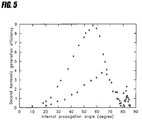
- Figure 5 illustrates exemplary Maker fringe profiles measured from a common sample 60 (shown as open circles) and from a composite sample 30 (shown as crosses).
- the measured fringe profile corresponds to the Fourier transform magnitude of the second-order optical nonlinearity profile of the composite sample 30.
- measuring the Fourier transform magnitude comprises measuring the Maker fringe profile of the composite sample 30.
- the composite sample 30 was formed by cutting the common sample 60 in half and placing the two halves proximate to one another with the surfaces near the poled regions in contact with one another.
- the fringe profile of the composite sample 30 is more intense and is shifted towards lower angles than that of the common sample 60 because the nonlinear region of the composite sample 30 is twice as thick as the nonlinear region of the common sample 60.
- Figure 6 illustrates the second-order nonlinearity profile d 33 ( z ) of the composite sample 30 obtained by calculating the inverse Fourier transform of the Fourier transform calculated using the measured fringe profile from the composite sample 30 as illustrated in Figure 5 .
- the nonlinearity profile of the composite sample 30 is the juxtaposition of the d 33 ( z ) profile of the sample 10 and its mirror image with respect to the origin, i.e., - d 33 (- z ), from the supplemental sample 20.
- the original nonlinearity profile d 33 ( z ) of the sample 10 is directly obtained, as illustrated in Figure 7 .
- the nonlinearity profile of Figure 7 represents an unambiguously derived nonlinearity profile of the thermally poled silica sample 10. The need for the phase information has been eliminated by artificially creating an odd nonlinearity profile based on the nonlinearity profile of the sample 10.
- Figure 7 also includes information regarding the depth location of the nonlinearity, which would not be available using prior methods, even if the phase information was retrieved.
- the peak of the nonlinearity profile is located approximately one micron under the anode surface, and the poled region extends approximately 35 microns under the surface.
- the main mechanism believed to be responsible for the second-order optical susceptibility ⁇ (2) in thermally poled silica is DC rectification of the third-order optical susceptibility ⁇ (3) of silica.
- the second-order susceptibility ⁇ (2) is proportional to ⁇ ( 3 ) E ( z ), where E ( z ) is the permanent electric field that develops inside the glass during poling.
- the nonlinearity profile derived in accordance with embodiments of the present invention can be independently verified by comparing the measured Maker fringe profile from the original sample 10 (shown as open circles in Figure 5 and Figure 8 ) with the theoretical fringe profile (solid curve in Figure 8 ) calculated from d 33 ( z ) obtained from the measured SH signal from the composite sample 30 ( Figure 7 ).
- This comparison illustrated in Figure 8 , shows that the two fringe profiles agree reasonably well, and that in particular, the spatial uniformity of the second-order susceptibility of the sample 10 was sufficient to infer the nonlinearity profile reliably.
- Embodiments of the present invention enable the second-order nonlinearity profile of an optically nonlinear film to be inferred unambiguously from a Maker fringe profile measurement.
- the nonlinearity profile of an exemplary thermally poled silica sample has been determined to: (i) have a peak value of approximately 0.8 pm/V, (ii) extend approximately 35 microns below the sample surface, and (iii) take both positive and negative values.
- Such magnitude and spatial information of the nonlinearity profile and of the charge distribution has significant implications in the design of future devices based on thermally poled silica.
- Embodiments described above can be considered to be special cases of a more general method of determining the second-order nonlinearity profile.
- the nonlinearity profile of a sample is uniquely determined without either of the two assumptions described above.
- the sample 10 need not be cut into two pieces to determine the nonlinearity profile.
- Figure 9 is a flow diagram of a method 150 of measuring a sample nonlinearity profile 15 of a sample 10.
- a sample 10 having at least one sample surface and having a sample nonlinearity profile 15 along a sample line through a predetermined point on the sample surface is provided. The sample line is oriented perpendicularly to the sample surface.
- a Fourier transform magnitude of the sample nonlinearity profile 15 is measured.
- a reference material having at least one reference surface and having a reference nonlinearity profile along a reference line through a predetermined point on the reference surface is provided. The reference line is oriented perpendicularly to the reference surface.
- a Fourier transform magnitude of the reference nonlinearity profile is obtained.
- a first composite sample having a first composite nonlinearity profile is formed. The first composite sample is formed by placing the sample 10 and the reference material proximate to one another in a first configuration with the sample line substantially collinear with the reference line.
- a Fourier transform magnitude of the first composite nonlinearity profile is measured.
- a second composite sample having a second composite nonlinearity profile inequivalent to the first composite nonlinearity profile is formed. The second composite sample is formed by placing the sample 10 and the reference material proximate to one another in a second configuration with the sample line substantially collinear with the reference line.
- a Fourier transform magnitude of the second composite nonlinearity profile is measured.
- the sample nonlinearity profile 15 is calculated using the Fourier transform magnitudes of the sample nonlinearity profile, the reference nonlinearity profile, the first composite nonlinearity profile, and the second composite nonlinearity profile.
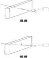
- the Fourier transform magnitude of the sample nonlinearity profile is measured in the operational block 154 by measuring the Maker fringe (MF) data of the sample in a single-pass configuration as schematically illustrated by Figure 10A .
- the MF data of the sample (MF 1 ) is thus representative of the Fourier transform magnitude of the sample nonlinearity profile along a sample line through a predetermined point (labelled "A" in Figure 10A ) on the sample surface.
- the sample line is oriented perpendicularly to the sample surface.
- the Fourier transform magnitude of the reference nonlinearity profile can be measured by measuring the MF data of the reference material in a single-pass configuration.
- the MF data of the reference material (MF 2 ) is thus representative of the Fourier transform magnitude of the reference nonlinearity profile along a reference line through a predetermined point (labelled "B" in Figure 10B ) on the reference surface.
- f is the spatial frequency.
- ⁇ is the fundamental wavelength
- n 1 , n 2 , ⁇ ⁇ , and ⁇ 2 ⁇ are the refractive indices and internal propagation angles at the fundamental and second harmonic wavelengths, respectively.
- d A (z) does not equal d B (z).
- W B depth of the poled region at the reference surface
- FIGs 11A-11D schematically illustrate various configurations for forming composite samples in accordance with embodiments of the present invention.
- Each of the composite samples of Figures 11A-11D has a corresponding composite nonlinearity profile.
- the composite sample is formed by placing the anodic surface of the sample and the anodic surface of the reference material proximate to one another, and is referred to herein as an anode-to-anode configuration.
- the composite sample is formed by placing the cathodic surface of the sample and the cathodic surface of the reference material proximate to one another, and is referred to herein as a cathode-to-cathode configuration.
- the composite sample is formed by placing the anodic surface of the sample and the cathodic surface of the reference material proximate to one another, and is referred to herein as an anode-to-cathode configuration.
- the composite sample is formed by placing the cathodic surface of the sample and the anodic surface of the reference material proximate to one another, and is referred to herein as a cathode-to-anode configuration.
- the Fourier transform magnitude of the first composite nonlinearity profile is measured in the operational block 162 ( Figure 9 ) by measuring the MF data of the first composite sample in a double-pass configuration.
- the MF data of the first composite sample is thus representative of the Fourier transform magnitude of the first composite nonlinearity profile along the dashed line of the corresponding one of Figures 11A-11D .
- the Fourier transform magnitude of the second composite nonlinearity profile is measured in the operational block 166 ( Figure 9 ) by measuring the MF data of the second composite sample in a double-pass configuration.
- the configuration of the second composite sample is chosen to provide a second composite nonlinearity profile inequivalent to the first composite nonlinearity profile. For example, if the first configuration of the first composite sample is that of Figure 11A or Figure 11B , then the second configuration of the second composite sample can be that of Figure 11C or Figure 11D . Similarly, if the first configuration of the first composite sample is that of Figure 11C or Figure 11D , then the second configuration of the second composite sample can be that of Figure 11A or Figure 11B .
- the MF data of the second composite sample is thus representative of the Fourier transform magnitude of the second composite nonlinearity profile along the dashed line of the corresponding one of Figures 11A-11D .
- the MF data of the anode-to-anode configuration of Figure 11A contains the same information as the MF data of the cathode-to-cathode configuration of Figure 11B (MF S2 ).
- the MF data of the anode-to-cathode configuration of Figure 11C contains the same information as the MF data of the cathode-to-anode configuration of Figure 11D (MF S4 ).
- M F S 1
- M F S 2
- M F S 3
- M F S 4
- Equation 5 From Equations 4 and 5, it can be seen that MF S1 and MF S2 are equivalent to one another (i.e., they have the same information in terms of ⁇ A and ⁇ B ).
- the extra modulation term ⁇ 0 2 ⁇ fL (where L is the sample thickness) does not contribute information regarding the nonlinearity profiles since it corresponds to a modulation term due to the summed thicknesses of the sample and reference material.
- the factor of 2 in front of ⁇ 0 comes from the assumption that the thickness of the sample and of the reference material are the both equal to L.
- MF S3 and MF S4 are equivalent to one another, but are inequivalent to MF S1 and MF S2 .
- either MF S1 or MF S2 is used as a first independent source of information
- either MF S3 or MF S4 is used as a second independent source of information.
- MF S1 or MF S2 is used as a first independent source of information
- MF S3 or MF S4 is used as a second independent source of information.
- the Fourier transforms of these functions are denoted as d S 1 z ⁇ FT D S 1 f and d S 2 z ⁇ FT D S 2 f .
- the Fourier transform magnitudes of the sample nonlinearity profile, the reference nonlinearity profile, the first composite nonlinearity profile, and the second composite nonlinearity profile are used to calculate the sample nonlinearity profile in the operational block 168.
- 2
- 2
- M F S 2
- 2
- 2
- 2
- ⁇ 0 ( f ) 2 ⁇
- M F S 2
- ⁇ A ⁇ ⁇ B 2 ⁇ ⁇ n ⁇
- m and n can take any integer value (0, ⁇ 1, ⁇ 2,). Note also that the output of the inverse cosine function is between 0 and ⁇ .
- ⁇ B ⁇ ⁇ 0 2 ⁇ ⁇ l ⁇ 1 2
- Equations 16 and 17 can be rewritten in the following form:
- Equations 18 and 19 provide useful information towards the calculation of the sample nonlinearity profile.
- P 2
- P 1 and P 2 denote these two possible values. Notice also that if
- P 1 , then
- P 2 . The reverse is also true, i.e., if
- P 2 , then
- P 1 .
- Equations 22 and 23 are connected to Equations 18 and 19 because of the
- This connection can be used to remove the final ambiguity of whether
- P 1 or
- P 2 . Since d A z + L 2 + d A ⁇ z + L 2 is a symmetric and real function, its Fourier transform magnitude is sufficient to uniquely recover it. The same is also true for d B z ⁇ L 2 + d B ⁇ z ⁇ L 2 , which is also a symmetric and real function.
- the Hartley transform is the same as the Fourier transform.
- the final ambiguity can then be removed using the Hartley transform, since for a real and compact support function (i.e., one that equals zero outside a finite region), the intensity of the Hartley transform is enough to uniquely recover the original function. See, e.g., N. Nakajima in Reconstruction of a real function from its Hartley-transform intensity, Journal of the Optical Society of America A, Vol. 5, 1988, pages 858-863 , and R.P. Millane in Analytic Properties of the Hartley Transform and their Implications, Proceedings of the IEEE, Vol. 82, 1994, pages 413-428 , both of which are incorporated in their entirety by reference herein.
- the ambiguity is removed in the following manner. If
- P 1 , then the function 2
- the ambiguity is removed by computing the inverse Fourier transform of the Fourier transforms obtained from both 2
- Figures 13A and 13B show arbitrarily selected nonlinearity profiles of the sample and the reference sample, respectively, and Figures 13C and 13D show the nonlinearity profiles of the two sandwich configurations, respectively.
- Figure 14A shows the calculated MF curves corresponding to the single-pass configuration of the sample (shown as a solid line) and the reference sample (shown, as a dashed line).
- Figure 14B shows the calculated MF curves corresponding to the double-pass configuration of the first sandwich configuration (shown as a solid line) and of the second sandwich configuration (shown as a dashed line).
- Figures 15A and 15B respectively show the original nonlinearity profiles d A (z) and d B (z) as solid curves, and show the corresponding profiles retrieved using the above-described method as crosses.
- the foregoing description includes ways to uniquely recover the two arbitrary nonlinearity profiles ( d A (z) and d B (z) ) using four sets of MF data. This result is significant since (1) the technique is applicable to even nonuniform poled samples; and (2) the sample does not need to be cut into two halves.
- the technique utilizes a reference material with known MF data.
- obtaining the MF data of the reference material comprises measuring the MF data.
- the MF data of the reference material is previously measured and stored in memory, and obtaining the MF data comprises reading the MF data from memory.
- Embodiments in which the MF data is previously stored are preferable, since the number of MF measurements will be reduced from 4 to 3. Note that it is not necessary to know the reference nonlinearity profile for this technique to work, since only its corresponding MF data is used.
- a common reference sample can be used to characterize a plurality of samples.
- C ⁇
- and ⁇ A ⁇ B .
- the MF data of the second composite sample (MF S2 , given by Equation 11) is not required to determine the sample nonlinearity profile.
- Equation 12 Equation 12 can be rewritten as: 2 ⁇
- M F 1 ⁇ 1 + C 2 ⁇ C ⁇ M F S 1 C
- Equation 25 The left-hand-side of Equation 25 is the Fourier transform magnitude of d A ( z ) + d A (- z ) and for such real and symmetric functions, the Fourier transform magnitude is sufficient to uniquely recover the original profile.
- MF S 1 4
- the nonlinear profile of the flipped sample d (- z ) changes sign to - d ( z ).
- the nonlinearity profile of the composite sample equals d ( z ) - d ( -z ).
- the effect of this sign change of the flipped sample is that the nonlinearity profile of the composite sample is now an odd function, i.e., it is symmetric about the origin.
- the Fourier transform is purely imaginary and odd, and the phase of the Fourier transform is equal to ⁇ /2.
- the Fourier transform of d ( z ) - d ( -z ) is 2 j
- the MF measurement provides a measurement of the Hartley transform magnitude of the real and odd function, i.e., the nonlinear profile of the composite sample d ( z ) - d (- z ).
- the retrieval of a real function from only its Hartley transform magnitude can be performed in various ways, as described by Nakajima and by Millane, as referenced above.
- the reference material can comprise a second sample with a second sample nonlinearity profile to be measured.
- the nonlinearity profiles of two samples can be measured concurrently.
- the same reference material can be used for measuring the nonlinearity profiles of a plurality of samples. If the same reference material is used with different samples, the measured reference nonlinearity profile should be substantially the same from each of the measurements. Comparison of the measured reference nonlinearity profiles accompanying each of the plurality of measured sample nonlinearity profiles then provides an indication of the consistency of the measurements across the plurality of samples.
- Figure 16 is a flow diagram of one embodiment of a method 170 of measuring a sample nonlinearity profile 15 of a sample 10.
- a sample 10 having at least one sample surface and having a sample nonlinearity profile along a sample line through a predetermined point on the sample surface is provided.
- the sample line is oriented perpendicularly to the sample surface.
- a reference material having at least one reference surface and having a reference nonlinearity profile along a reference line through a predetermined point on the reference surface is provided.
- the reference line is oriented perpendicularly to the reference surface.
- a first composite sample having a first composite nonlinearity profile is formed.
- the first composite sample is formed by placing the sample 10 and the reference material proximate to one another in a first configuration with the sample line substantially collinear with the reference line.
- a Fourier transform magnitude of the first composite nonlinearity profile is measured.
- a second composite sample having a second composite nonlinearity profile inequivalent to the first composite nonlinearity profile is formed.
- the second composite sample is formed by placing the sample 10 and the reference material proximate to one another in a second configuration with the sample line substantially collinear with the reference line.
- a Fourier transform magnitude of the second composite nonlinearity profile is measured.
- the sample nonlinearity profile 15 is calculated using the Fourier transform magnitudes of the first composite nonlinearity profile and the second composite nonlinearity profile.
- Figure 17 is a flow diagram of one embodiment of the operational block 177 for calculating the sample nonlinearity profile 15.
- an inverse Fourier transform of the difference between the Fourier transform magnitudes of the first and second composite nonlinearity profiles is calculated.
- the inverse Fourier transform is separated into a first convolution function and a second convolution function.
- the Fourier transform of the first convolution function and the Fourier transform of the second convolution function are calculated.
- the phase and amplitude of the Fourier transform of the sample nonlinearity profile are calculated using the Fourier transforms of the first and second convolution functions.
- the inverse Fourier transform of the Fourier transform of the sample nonlinearity profile 15 is calculated.
- the nonlinearity profile of the sample can be computed in the following manner.
- the nonlinear coefficient profiles of sample A and B are defined as d A ( z ) and d B ( z ), respectively, where z is in the direction perpendicular to the sample (see Figures 13A and 13B ).
- the respective thicknesses of the nonlinear regions in samples A and B are referred to as W A and W B , respectively.
- L G the thickness of the space between sample A and sample B (which can contain an index-matching gel)
- L L B + L G
- L B is the thickness of sample B.
- d S 1 ( z ) since sample B is flipped over, its nonlinearity profile has a negative sign. The physical reason for this sign change is that during poling the symmetry of the intrinsic material is broken along the z direction.
- the MF curves of S1 and S2 are proportional to the square of the FT magnitude of d S 1 ( z ) and d S 2 ( z ), respectively:
- M F S 1
- M F S 2
- the procedure to obtain the profiles d A ( z ) and d B ( z ) from the measured MF curves of S1 and S2 is as follows.
- the first step is to compute numerically the inverse Fourier transform of the difference MF S 2 - MF S 1 .
- the Fourier transform phases ⁇ A ( f ) and ⁇ B ( f ) are retrieved by computing the Fourier transforms of C 1 ( z ) and C 2 ( z ), which are equal to
- the phases ⁇ A ( f ) and ⁇ B ( f ) are then inserted into Equations 28 and 29, which are solved to obtain the Fourier transform amplitudes
- the final step is to take the inverse Fourier transform of the recovered quantities
- C 1 ( z ) and C 2 ( z ) can still be recovered by using a slightly different procedure that utilizes all four MF curves ( MF A , MF B MF S 1 , and MF S 2 ).
- the z ⁇ 0 portion of the inverse Fourier transform of ⁇ - MF S 1 + MF A + MF B ⁇ equals C 1 ( z + L G )
- the z ⁇ 0 portion of the inverse Fourier transform of ⁇ MF S 2 - MF A - MF B ⁇ equals C 2 ( z + L ).
- This property is used to retrieve the convolution functions C 1 (z) and C 2 ( z ), and the rest of the procedure is the same as described above.
- two Infrasil wafers (Samples A and B, each 25 mm x 25 mm x 1 mm) were thermally poled under nominally identical conditions (5 kV at approximately 270°C for 15 minutes).
- Sample B was polished down on its cathode side to a thickness L B of approximately 100 microns to reduce the spacing between the two nonlinear regions in the second composite sample S2, thereby reducing the frequency of oscillations at high angles in MF S2 , which would make its measurement unnecessarily difficult.
- a pair of Infrasil half-cylinders were clamped on each side of the wafer to avoid total internal reflection and achieve high incidence angles.
- Figures 18A-18D illustrate the measured MF curves shown as open circles with the second harmonic generation efficiency plotted against the incidence angle squared ( ⁇ 2 ), to better illustrate details at high angles.
- the insets of Figures 18A-18D schematically illustrate the geometry of the various samples.
- MF S2 oscillates prominently, as expected, since the two nonlinear regions in S2 are spaced a sizable distance (L approximately equal to 140 microns).
- the nonlinearity strength of polished Sample B is comparable to that of unpolished Sample A. This observation suggests that there is no significant induced nonlinearity in the bulk of the material or close to the cathode surface.
- Figure 19 illustrates the recovered sample nonlinearity profiles for Sample A and Sample B.
- the nonlinear coefficients peak at about one micron below the anode surface, with values of approximately 0.9 pm/V for d A (z) and approximately 1.0 pm/V for d B (z).
- the two profiles are similar in shape and magnitude, which is expected since they were poled under identical conditions. The difference between the locations of the negative peaks may be due to small variations in poling conditions. Since d A (z) and d B (z) are quite similar, it is also possible to retrieve these profiles by assuming that they are identical and applying the embodiment described above in relation to Figure 9 .
- the nonlinearity profile recovered in this fashion is also shown in Figure 19 .
- this profile is similar to both d A (z) and d B (z).
- the positive peak of this profile is nearly identical to those of d A (z) and d B (z)
- the negative peak of this profile provides an effective average of those of d A (z) and d B (z).
- a measured MF data curve does not provide the low and high frequency ends of the Fourier transform spectrum.
- the resulting abrupt discontinuities in the Fourier transform data in these regions introduce artificial oscillations in the inferred profiles.
- d A (z) and d B (z) , C 1 (z) , and C 2 ( z ) are zero outside a finite region and are square-integrable, their Fourier transforms are entire functions, which implies that in principle the whole Fourier transform can be reconstructed uniquely from the knowledge of the Fourier transform in a finite frequency range, as described by Millane, referenced herein.
- One implementation of this principle is the Papoulis-Gerchberg algorithm, described by P.J.S.G. Ferreira in IEEE Transactions on Signal Processing, 1994, Volume 42, page 2596 , incorporated in its entirety by reference herein, which can be used to extrapolate the measured data into the unmeasured low and high frequency end portions of the Fourier spectrum.
- this embodiment utilizes the measurement of two MF data curves, it is not any more labor-intensive than embodiments which utilize only one measurement, since it provides two profiles instead of a single one. Furthermore, after a pair of nonlinear samples have been characterized in this manner, either one of the two samples can be used as a reference sample with a known profile for measuring the profile of any other nonlinear sample, thereby using only a single new MF measurement (e.g., MF S2 ). Data processing for this single-measurement case is slightly different and even simpler.
- C 2 ( z ) can be retrieved unambiguously from the z ⁇ 0 portion of the inverse Fourier transform of MF S2 . Since the nonlinearity profile d A (z) of the reference sample is known, the Fourier transform of C 2 (z) (i.e.,
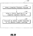
- FIG. 20 is a flowchart of a method 200 in accordance with embodiments of the present invention.
- a symmetric composite function is formed.
- a Fourier transform of the symmetric composite function is obtained.
- an inverse Fourier transform of the obtained Fourier transform is calculated. The calculated inverse Fourier transform provides information regarding the physical function.
- the symmetric composite function is an odd function (i.e., is symmetric about the origin). In other embodiments, the symmetric composite function is even (i.e., symmetric about the y-axis). In certain embodiments, obtaining the Fourier transform of the composite function comprises obtaining a Fourier transform magnitude of the composite function and using the Fourier transform magnitude to calculate the Fourier transform of the composite function.
- a symmetric composite function in the spatial domain as described above in relation to the nonlinearity profile of poled silica
- other embodiments form a symmetric intensity profile in the time domain by the use of time reversal.
- the symmetric (even) composite function can have utility where phase information is needed but unavailable (e.g., ultra-short pulse diagnosis using auto-correlators).
- time reversal is described by D.A.B. Miller in -Time Reversal of Optical Pulses by Four-Wave Mixing, Optics Letters Vol. 5, 1980, pages 300-302 , which is incorporated in its entirety by reference herein.
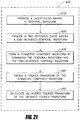
- Figure 21 is a flow diagram of a method 400 of determining the temporal waveform 312 of a laser pulse 310 in accordance with embodiments of the present invention.
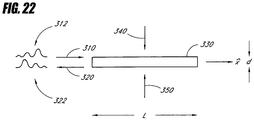
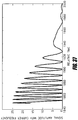
- Figure 22 schematically illustrates one configuration for utilizing four-wave mixing (FWM) to provide the time-reversed pulse 320 in accordance with embodiments of the present invention. Other configurations are also compatible with the method of Figure 21 .
- FWM four-wave mixing
- FIG. 22 in an operational block 410, a laser pulse 310 is provided.
- the laser pulse 310 has a temporal waveform 312.
- a time-reversed pulse 320 is provided in an operational block 420.
- the time-reversed pulse 320 has a time-reversed temporal waveform 322 which corresponds to the temporal waveform 312 after being time-reversed.
- the temporal waveform 312 of the laser pulse 310 and the time-reversed temporal waveform 322 of the time-reversed pulse 320 form a symmetric composite waveform.
- a Fourier transform of the symmetric composite waveform is obtained.
- obtaining the Fourier transform of the symmetric composite function comprises measuring a Fourier transform magnitude of the symmetric composite function, and using the measured Fourier transform magnitude to calculate the Fourier transform of the symmetric composite function.
- an inverse Fourier transform of the obtained Fourier transform is calculated. The calculated inverse Fourier transform provides information regarding the temporal waveform 312 of the laser pulse 310.
- FWM has been a subject of interest in applications such as aberration compensation, spatial information processing, frequency filtering, pulse envelope shaping, and dispersion compensation.
- a nonlinear medium 330 of length L is pumped by two pulsed pump waves 340, 350.
- An input laser pulse 310 (with temporal waveform 312 given by E p ( x , t )) launched into the nonlinear medium 330 generates a phase conjugate pulse 320 (with time-reversed temporal waveform 322 given by E c ( x , t )), which is the time-reversed version of the temporal waveform 312 of the input pulse 310.
- the input pulse 310, two pump waves 340, 350, and the nonlinear medium are at the same place for the duration of the input pulse 310.
- the input pulse 310, and the two pump waves 340, 350 overlap in the frequency domain.
- u p ( t ) is the modulation of the carrier e j ( ⁇ p t - k x) .
- the foregoing forms of the envelope function u c ( t ) were obtained using the teachings of R.A. Fischer et al. in Transient Analysis of Kerr-Like Phase Conjugators Using Frequency-Domain Techniques, Physical Review A, Vol. 23, 1981, pages 3071-3083 , which is incorporated in its entirety by reference herein.
- Equation 40 u c ( t )
- K ' and ⁇ 0 constants.
- the - t term in Equation 40 indicates the time reversal operation. Note that Equation 33 and Equation 37 are still valid for this case.
- the assumptions made in the derivation of Equation 40 are that:
- the time-reversed pulse 320 can be provided using holographic techniques in accordance with embodiments of the present invention.
- Femtosecond spectral holography can be considered as a temporal analog of the classical spatial domain holography.
- classical holography a spatial information carrying beam (signal) and a uniform reference beam interfere in a recording medium, thereby recording a hologram comprising a set of fringes. Illumination of the hologram with a uniform test beam reconstructs either a real or conjugate image of the signal beam, depending on the geometry.
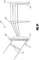
- Femtosecond spectral holography for the time reversal process comprises a recording phase and a read-out phase, as schematically illustrated respectively by Figures 23A and 23B .
- the reference pulse 360 is short with a relatively flat and broad spectrum
- the input pulse 310 has a temporal waveform 312 that has a shape indicative of information carried by the input pulse 310.
- a grating 370 is used to disperse both the reference pulse 360 and the input pulse 310 into their spectral components, which then propagate through a collimating lens system 372.
- the interference pattern formed by the complex amplitudes of each spectral component is then recorded in the holographic recording plate 375.
- a short test pulse 380 is dispersed by the grating 370 and then recollimated by the lens 372.
- the illumination of the holographic plate 375 with this recollimated dispersed test beam 392 produces the beam 396.
- a time-reversed replica 390 of the original input pulse 310 is produced.
- the transmitted test beam 392 appears at the output.
- the envelope of the output pulse 390 can be expressed as: u out t ⁇ u t t ⁇ u r ⁇ t ⁇ u s t e j K ⁇ 1 r ⁇ + u t t ⁇ u r t ⁇ u s ⁇ t e j K ⁇ 1 r ⁇
- u out ( t ), u t ( t ), u r ( t ), and u s ( t ) are the complex envelope functions of the electric fields of the output pulse 390, test pulse 380, reference pulse 360, and input pulse- 310, respectively.
- the complex envelope functions u s ( t ), u t ( t ), and u r ( t ) will act as delta functions with respect to u s ( t ), modifying the envelope of the output pulse 390 to be: u out t ⁇ u s t e j K ⁇ 1 r ⁇ + u s ⁇ t e j K ⁇ 2 r ⁇ . Therefore, as a result of the illumination of the holographic plate with the test pulse 380, the output pulse 390 serves as the time-reversed signal pulse 320 in the K 2 direction.
- the apparatus schematically illustrated by Figures 23A and 23B can serve as a phase conjugate mirror which generates the time-reversed waveform corresponding to an input waveform.
- pulse-pumped FWM uses shorter pulses than the input pulse 310 to time-reverse the input pulse 310.
- shorter pump pulses 340, 350 are used, and for holography, shorter test pulses 380 and reference pulses 360 are used.
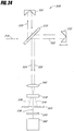
- Figure 24 schematically illustrates one embodiment of a classical intensity correlator utilizing a Michelson interferometer 500 in combination with a second-harmonic generating (SHG) crystal 510 to estimate the temporal waveform of a laser pulse.
- the input pulse 310 is split into a first pulse 520 and a second pulse 522 by the beamsplitter 530.
- the first pulse 520 is reflected by a fixed mirror 550 back through the beamsplitter 530, thereby transmitting a third pulse 524.
- the second pulse 522 is reflected by a movable mirror 552 back through the beamsplitter 530, thereby transmitting a fourth pulse 526 towards the focusing lens 540.
- the movable mirror 552 adds a variable delay ⁇ to the fourth pulse 526 with respect to the third pulse 524.
- the focusing lens 540 focuses the third pulse 524 and the fourth pulse 526 onto the SHG crystal 510.
- the SHG crystal 510 generates a second-harmonic (SH) field 538 which is a cross-correlation product of the third pulse 524 and the fourth pulse 526.
- SH fields 534, 536 generated by the SHG crystal 510 do not carry information regarding the third and fourth pulses 524, 526 simultaneously, and these other SH fields are blocked by the pinhole 560 placed after the SHG crystal 510.
- the cross-correlation product 538 is detected by a photomultiplier tube 580.
- the signal detected by the photomultiplier 580 (i.e., the autocorrelation function) is given by:
- 2 dt
- I ( t )
- u i ( t ) ⁇ U i ( ⁇ ) e j ⁇ t d ⁇ .
- ⁇ is constant over the frequency range of the combined pulses, which is equivalent to assuming that ⁇ (2) is independent of frequency. This assumption holds when the effective crystal length is shorter than the coherence length of the harmonic generation over the pulse bandwidth.
- the signal from the Michelson interferometer 500 of Figure 24 provides the magnitude of the Fourier transform of the input pulse intensity I ( t ).
- the magnitude of the Fourier transform is not sufficient information to retrieve uniquely the input pulse intensity I(t). To do so would also require the knowledge of the phase of the Fourier transform, which this classical autocorrelation method does not provide.
- This difficulty in uniquely determining the input pulse intensity I(t) is analogous to that of retrieving the second-order susceptibility spatial profile of a nonlinear material, as described above.
- a number of methods can be used to avoid this difficulty. For example, a certain shape for the pulse intensity (e.g., a Gaussian) can be assumed, but there is no way to independently verify that the assumed shape is the true temporal waveform. This method therefore provides only an estimate of the pulse shape.
- a time-reversed pulse with a time-reversed temporal waveform I (- t ) of the temporal waveform I ( t ) of an arbitrary pulse can be produced.
- a symmetric composite waveform can then be formed by delaying the time-reversed pulse with respect to the original pulse and combining the temporal waveform with the time-reversed temporal waveform, for example with a beamsplitter.
- Figure 25 schematically illustrates a general configuration 600 for converting a periodically repeated sequence of pulses into a periodically repeated sequence of symmetric pulses using a movable phase conjugative mirror 610.
- the input pulse sequence 620 comprises a series of original pulses 622.
- the original pulses 622 can be symmetric or asymmetric.
- Each of these original pulses 622 is split by the beamsplitter 630 into two portions 640, 642, with one portion 640 being reflected by a phase conjugate mirror 610.
- the phase conjugate mirror 610 comprises an apparatus as schematically illustrated by Figure 22 in which the input pulse 310 is used to generate the output pulse 320.
- the phase conjugate mirror 610 comprises an apparatus as schematically illustrated by Figures 23A and 23B in which the input pulse 310 is used to generate the output pulse 390.
- the portions 640, 642 are combined to form a symmetric composite waveform 650 comprising the temporal waveforms of the original pulses 622 and of the corresponding phase conjugate (time-reversed) pulses 652.
- the amount of delay ⁇ t between an original pulse 622 and the corresponding time-reversed pulse 652 in the symmetric pulse sequence 650 is adjustable by moving the phase conjugative mirror 610.
- Equation 50 provides the intensity of the symmetric pulse sequence 650 without any ambiguity. Once the intensity of the symmetric pulse sequence 650 is calculated in this way, the intensity of the original pulse can be found by separating the pulse 650 in the middle.
- Figure 26 illustrates an exemplary temporal waveform of an input pulse 622 compatible with embodiments of the present invention.
- the autocorrelation technique commonly used to estimate the temporal profile of an optical pulse is applied to this input pulse as follows.
- the autocorrelation function (Equation 46) corresponding to the temporal waveform is measured.
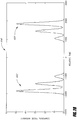
- the magnitude of the Fourier transform of the signal A PMT_single ( ⁇ ) recorded by the photomultiplier tube 580 is schematically illustrated in Figure 27 .
- the frequency f shown in Figure 27 is 1/ ⁇ , and is not to be confused with the optical frequency.
- Figure 28 illustrates the symmetric composite waveform 650 defined by Equation 48, which is obtained by combining the input pulse and the time-reversed pulse.
- the symmetric composite waveform 650 comprises the temporal waveform of the original pulse 622 of Figure 25 plus the time-reversed temporal waveform of the corresponding time-reversed pulse 652, separated by some time delay.
- the autocorrelator of Figure 24 is used to generate the autocorrelation function corresponding to the symmetric composite waveform 650.
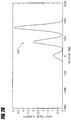
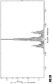
- Figure 29 illustrates the magnitude of A PMT_double ( f ) (expressed by Equation 50), which is the Fourier transform of the measured A PMT_double ( ⁇ ).
- the envelope of the Fourier transform magnitude of the measured A PMT_double ( ⁇ ) is a scaled version of the Fourier transform magnitude (as shown in Figure 27 ) of the signal A PMT _ single ( ⁇ ) measured by the photomultiplier tube 580.
- can be determined. Using Equation 49, the Fourier transform of the symmetric temporal waveform can be expressed as: I ⁇ symmetric f 2
- the Fourier transform I symmetric ( f ) is equivalent to the Hartley transform I symmetric Ha f . Therefore, the magnitude of the Hartley transform of I symmetric ( t ) (i.e.,
- 2
- ) can be determined from the knowledge of
- Figure 30A illustrates the recovered symmetric temporal waveform
- Figure 30B illustrates the difference between the recovered symmetric temporal waveform and the temporal waveform of the original pulse (as shown in Figure 28 ).
- the two waveforms are in excellent agreement (within approximately - 0.15) with one another.
- the difference shown in Figure 30B is in fact just a numerical calculation artifact, which can be improved with increased accuracy.
- the configuration schematically illustrated in Figure 24 is capable of recovering ultra-short temporal waveforms unambiguously when used with a time-reversal scheme, such as that illustrated by Figure 25 .
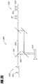
- Figure 31 schematically illustrates a system 700 for another embodiment for determining the temporal waveform of a laser pulse.
- the input pulse 710 impinges onto a grating 720 which disperses the input pulse 710 into its spectral components.
- a lens 730 recollimates the spectral components and images them onto different elements of a CCD imaging device 740.
- the input pulse 710 is decomposed by the grating 720 into several monochromatic plane waves with amplitudes ⁇ s ( ⁇ - ⁇ c ). By finding the response of the system 700 to each individual harmonic component (i.e. ⁇ s ( ⁇ - ⁇ c ) e j ⁇ t ), the overall response of the system 700 can be determined using the integral given in Equation 53.
- w ( x ) is the pupil function of the optical field on the grating 720
- c is the speed of light
- x is the coordinate along the plane 722
- ⁇ is the incident angle of the input pulse 710 to the grating 720.
- Equation 54 accounts for the diffraction experienced by the spectral components of the input pulse 710 due to the grating 720, assuming only first-order diffraction.
- the lens 730 transforms the image at the plane 722 into an image at plane 742.
- the fields at the two planes 722, 742 are related by a spatial Fourier transform.
- W ( f x' ) is the spatial Fourier transform of w ( x ).
- x' is the coordinate along the plane 742
- Equation 57 can be simplified to the following form: u 2 s x ′ ; t ⁇ U ⁇ s ⁇ x ′ ⁇ c F sin ⁇ w 1 ⁇ x ′ F sin ⁇ ct sin ⁇ e j ⁇ c 1 x ′ F sin ⁇ t .
- the function u PC ( t ) is dependent on the type of phase conjugate mirror used to generate the phase conjugate pulses.
- the resultant image field at the plane 742 of the CCD imaging device 740 can be expressed as: u total ,2 x ′ ; t ⁇ U ⁇ s ⁇ x ′ ⁇ c F sin ⁇ w 1 ⁇ x ′ F sin ⁇ ct sin ⁇ e j ⁇ c 1 ⁇ x ′ F sin ⁇ ′ t + U ⁇ s * ⁇ x ′ ⁇ c F sin ⁇ w 1 ⁇ x ′ F sin ⁇ ct sin ⁇ e j ⁇ c 1 ⁇ x ′ F sin ⁇ t e j ⁇ t x ′ ⁇ c F sin ⁇ .
- ⁇ s ( ⁇ )
- e j ⁇ ( ⁇ ) and A - F sin ⁇
- with G x ′ ⁇
- Equation 63 is very similar to Equation 50, which was obtained for embodiments utilizing the intensity correlator of Figure 24 .
- Equation 64 is also very similar to Equation 47, which was derived above in relation to the intensity correlator embodiment as shown in Figure 24 .
- Figures 32A and 32B illustrate the magnitude (intensity) and phase of an arbitrary asymmetric complex envelope function ⁇ s ( t ) to be characterized, respectively.
- Figure 32A is the same input pulse as shown in Figure 26 ).
- Figure 33 illustrates the intensity profile for this complex field, including the carrier frequency oscillations. Note that Figure 26 described above did not include the carrier frequency oscillations and was just the envelope of the intensity.
- the general configuration 600 of Figure 25 is used to generate the symmetric temporal waveform whose complex envelope function is defined by Equation 59.
- Figure 34 illustrates the symmetric temporal waveform, including the carrier frequency, generated by this first step.
- the symmetric temporal waveform comprises the temporal waveform of the original pulse plus the time-delayed temporal waveform of the time-reversed pulse.
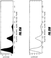
- Figure 35A illustrates the detected intensity I ( x' ) on the CCD imaging device at the plane 742 for the symmetric pulse of Figure 34 .
- the intensity I ( x' ) was calculated using Equation 63.
- Figure 35B shows the detected intensity I ( x ') on the CCD imaging device at the plane 742 using the original pulse of Figure 33 , which is a prior art measurement technique.
- the intensity I ( x ') was calculated using Equation 64.
- the CCD image ( Figure 35A ) is used to calculate numerically both amplitude and the phase of the Fourier transform of, the complex envelope function ⁇ s ( t ).
- the complex envelope function ⁇ s ( t ) can be calculated using inverse Fourier transform once both the amplitude and the phase functions of the Fourier transform are recovered.
- Figures 36A and 36B illustrate the recovered symmetric temporal waveform and the original temporal waveform, respectively, including the carrier frequencies.
- Figure 37 illustrates these waveforms overlaid with one another in an expanded time frame for comparison purposes. This comparison establishes that the prediction of the pulse shape made available by this invention is excellent.
- the discrepancy between the two curves of Figure 37 is in fact a numerical artifact that can be removed by increasing the computation accuracy.
- the system 700 of Figure 31 can be used to recover the complex envelope function ⁇ s ( t ) of any given input pulse using only the Fourier transform amplitude of the symmetrized composite waveform.
- both the envelope of the intensity profile I ( t ) and the underlying optical oscillations are recoverable, as illustrated by Figure 37 . Recovering both the envelope and the underlying oscillations is an improvement with respect to the prior art intensity correlation embodiment described above, which only recovers the envelope of I ( t ).
- the waveform of an ultra-short optical pulse is determined in certain embodiments by using time-reversal techniques to yield a time-reversed replica of the pulse and to obtain a symmetric optical pulse.
- the Fourier transform magnitude of the symmetric optical pulse is used to uniquely recover the original time-domain optical pulse waveform.
- Such time-reversal techniques utilize shorter optical pulses with respect to the input optical pulse waveform being measured. For example, to determine the temporal pulse waveform of a femtosecond-scale optical pulse, sub-femtosecond-scale pulses are used to form the symmetric optical pulse waveform by time reversal.
- FIG. 38 is a flow diagram of a method 800 in accordance with embodiments of the present invention.
- a sample optical pulse having a sample temporal waveform is provided.
- a Fourier transform magnitude of the sample temporal waveform is measured.
- a reference optical pulse having a reference temporal waveform is provided.
- a Fourier transform magnitude of the reference temporal waveform is obtained.
- a first composite optical pulse having a first composite temporal waveform is formed.
- the first composite optical pulse comprises the sample optical pulse followed by the reference optical pulse.
- a Fourier transform magnitude of the first composite temporal waveform is measured.
- a time-reversed optical pulse having a time-reversed temporal waveform is provided.
- the time-reversed temporal waveform corresponds to the reference temporal waveform after being time-reversed.
- a second composite optical pulse having a second composite temporal waveform is formed.
- the second composite optical pulse comprises the sample optical pulse followed by the time-reversed optical pulse.
- a Fourier transform magnitude of the second composite temporal waveform is measured.
- the sample temporal waveform is calculated using the Fourier transform magnitude of the sample temporal waveform, the Fourier transform magnitude of the reference temporal waveform, the Fourier transform magnitude of the first composite temporal waveform, and the Fourier transform magnitude of the second composite temporal waveform.
- the sample optical pulse of certain embodiments can have an ultra-short temporal waveform (e.g., on the order of femtoseconds or sub-femtoseconds).
- the reference optical pulse of certain embodiments can have a temporal waveform which is significantly more broad than the temporal waveform of the sample optical pulse. For example, for a femtosecond sample temporal waveform, the width of the reference temporal waveform can be on the order of nanoseconds.
- the first composite optical pulse includes a time delay between the sample optical pulse and the reference optical pulse.
- the time delay can be adjusted to make the measurement of the Fourier transform magnitude easier.
- the time delay used can be dependent upon the particular technique used to measure the Fourier transform magnitude.
- the second composite optical pulse includes a time delay between the sample optical pulse and the time-reversed optical pulse, and the time delay can be adjusted to ease the measurement of the Fourier transform magnitude depending on the particular measurement technique used.
- the Fourier transform magnitudes of the sample temporal waveform, the reference temporal waveform, the first composite temporal waveform, and the second composite temporal waveform are measured using an autocorrelator as described above, or using other holographic techniques.
- obtaining the Fourier transform magnitude of the reference temporal waveform comprises measuring the Fourier transform magnitude.
- the Fourier transform magnitude of the reference temporal waveform is previously measured and stored in memory, and obtaining the Fourier transform magnitude comprises reading the Fourier transform magnitude from memory.
- the sample temporal waveform can be measured.
- the reference temporal waveform can also be calculated by embodiments of the present invention concurrently with the calculation of the sample temporal waveform.
- the reference optical pulse is temporally broad, its temporal waveform is of less interest than that of the sample optical pulse.
- the calculated series of reference temporal waveforms can be compared to one another, thereby providing a check of the validity of the measurements across the series of calculations.
- the quantities of interest are by definition real and positive.
- two totally arbitrary and different ultra-short pulse waveforms can be used together to determine the pulse profiles I A (t), I B (t) of both pulses.
- a classical autocorrelator can be used to generate the Fourier transform amplitudes of the pulse waveforms.
- Time reversal techniques are utilized in such embodiments due to the I B (-t+ ⁇ 2 ) term.
- the time reversal is simpler to achieve to determine the pulse shape of an ultra-short sample pulse waveform.
- FIG 39 is a flow diagram of a method 1000 in accordance with certain embodiments of the present invention.
- a sample pulse waveform having a sample temporal waveform is provided.
- a reference pulse waveform is provided.
- a composite temporal waveform is formed.
- the composite temporal waveform comprises the sample pulse waveform and the reference pulse waveform with a relative delay between the sample pulse waveform and the reference pulse waveform.
- a Fourier transform magnitude squared of the composite temporal waveform is measured.
- an inverse Fourier transform of the measured Fourier transform magnitude squared is calculated.
- the sample temporal waveform is calculated using the calculated inverse Fourier transform.
- the Fourier transform magnitude squared of the composite waveform is expressed as Equation 68.
- the operational block 1050 then comprises calculating an inverse Fourier transform of the measured Fourier transform magnitude squared.
- I Ref (t) is a real, even, and non-negative function
- its Fourier transform is also real and even, meaning that ⁇ Ref equals either 0 or ⁇ .
- ⁇ Ref can be fully determined using only the information of
- the phase of the Fourier transform of Conv(t) can be used to determine the phase ⁇ of the Fourier transform of I(t), the sample pulse waveform.
- I ( f )
- e j ⁇ is recovered, and by taking the inverse Fourier transform, the sample pulse waveform I(t) can be determined.
- the method described above can be used to determine the temporal shape of an ultra-short sample pulse waveform using a symmetric unchirped reference pulse waveform using only one measurement (e.g., an auto-correlator measurement).
- the recovery of the sample pulse waveform using the method described above is robust, even in the presence of noise added to the measured Fourier transform magnitudes.
- the laser can then be used to characterize other pulsed laser sources, even though neither laser has symmetric output pulses. For example, after an initial measurement to characterize a non-symmetric sample pulse waveform using an unchirped symmetric pulse, one can continue to characterize different pulse waveforms using the non-symmetric pulse waveform that has been previously characterized as the reference pulse waveform for the subsequent measurements.
Landscapes
- Physics & Mathematics (AREA)
- General Physics & Mathematics (AREA)
- Engineering & Computer Science (AREA)
- Mathematical Physics (AREA)
- Theoretical Computer Science (AREA)
- Mathematical Analysis (AREA)
- Mathematical Optimization (AREA)
- Pure & Applied Mathematics (AREA)
- Computational Mathematics (AREA)
- Health & Medical Sciences (AREA)
- Data Mining & Analysis (AREA)
- Databases & Information Systems (AREA)
- Chemical & Material Sciences (AREA)
- General Engineering & Computer Science (AREA)
- Discrete Mathematics (AREA)
- Nonlinear Science (AREA)
- Optics & Photonics (AREA)
- Algebra (AREA)
- Nuclear Medicine, Radiotherapy & Molecular Imaging (AREA)
- Life Sciences & Earth Sciences (AREA)
- Software Systems (AREA)
- Analytical Chemistry (AREA)
- Biochemistry (AREA)
- General Health & Medical Sciences (AREA)
- Immunology (AREA)
- Pathology (AREA)
- Spectroscopy & Molecular Physics (AREA)
- Investigating Or Analysing Materials By Optical Means (AREA)
- Photometry And Measurement Of Optical Pulse Characteristics (AREA)
- Length Measuring Devices By Optical Means (AREA)
- Image Analysis (AREA)
Claims (4)
- Verfahren zum Bestimmen einer zeitlichen Wellenform I(t) eines optischen Pulses, wobei das Verfahren umfasst:Erhalten einer symmetrischen zusammengesetzten Funktion I symmetrisch (t), die der zeitlichen Wellenform des optischen Pulses plus einer zeitumgekehrten zeitlichen Wellenform des optischen Impulses entspricht, wobei

 Δt eine variable Zeitverzögerung zwischen dem optischen Puls und einem zeitumgekehrten optischen Puls ist, welcher die zeitumgekehrte zeitliche Wellenform aufweist;Erhalten der gemessenen Autokorrelierungsfunktion APMT_dopper (τ) der symmetrischen zusammengesetzten Funktion I symmetrisch (t);Erhalten einer Fourier-Transformation
A PMT_doppel (f) der gemessenen Autokorrelationsfunktion, wobeiA PMT_doppel (f)= 2|η|2|I (f)|2|1+cos(2ϕ(f)- fΔt)|, wobei η konstant angenommen wird;Wiederherstellen von |I (f)|2 aus der Umhüllenden vonA PMT_doppel (f) ;Bestimmen einer Funktion g(f) = 1 + cos(2ϕ(f)- f(Δt) durch Dividieren der Fourier-Transformation der AutokorrelierungsfunktionA PMT_doppel (f) durch |I ((f)|2 undBestimmen eines Terms falls keine Nulldurchgänge des Terms
 Berechnen einer inversen Fourier-Transformation von

 falls Nulldurchgänge des Terms
 Bestimmen eines Betrags einer Hartley-Transformation der symmetrischen zusammengesetzten Funktion I symmetrisch (t) aus

I (f)|, um I symmetrisch (t) zu bestimmen; undBestimmen der zeitlichen Wellenform I(t) durch Trennen von I symmetrisch (t) in die zeitliche Wellenform und die zeitumgekehrte zeitliche Wellenform. - Verfahren nach Anspruch 1, wobei der optische Impuls ein Laserimpuls ist.
- Verfahren nach einem der vorhergehenden Ansprüche, wobei die zeitliche Wellenform symmetrisch ist.
- Verfahren nach Anspruch 1 oder 2, wobei die zeitliche Wellenform nicht symmetrisch ist.
Applications Claiming Priority (5)
| Application Number | Priority Date | Filing Date | Title |
|---|---|---|---|
| US40540502P | 2002-08-21 | 2002-08-21 | |
| US10/357,275 US7133134B2 (en) | 2002-08-21 | 2003-01-31 | Method of measuring a physical function using a symmetric composite function |
| US10/378,591 US6856393B2 (en) | 2002-08-21 | 2003-03-03 | Method of measuring a physical function using a composite function which includes the physical function and an arbitrary reference function |
| EP03793270A EP1530712B1 (de) | 2002-08-21 | 2003-08-21 | Verfahren zur Messung optischer Nichlinearitätsraumprofile von Proben |
| PCT/US2003/026311 WO2004019018A2 (en) | 2002-08-21 | 2003-08-21 | Method of measuring nonlinearity spatial profiles of samples and temporal profiles of optical pulses |
Related Parent Applications (2)
| Application Number | Title | Priority Date | Filing Date |
|---|---|---|---|
| EP03793270.4 Division | 2003-08-21 | ||
| EP03793270A Division EP1530712B1 (de) | 2002-08-21 | 2003-08-21 | Verfahren zur Messung optischer Nichlinearitätsraumprofile von Proben |
Publications (3)
| Publication Number | Publication Date |
|---|---|
| EP2278302A2 EP2278302A2 (de) | 2011-01-26 |
| EP2278302A3 EP2278302A3 (de) | 2012-08-01 |
| EP2278302B1 true EP2278302B1 (de) | 2018-12-12 |
Family
ID=46123495
Family Applications (3)
| Application Number | Title | Priority Date | Filing Date |
|---|---|---|---|
| EP10010839.8A Expired - Lifetime EP2278302B1 (de) | 2002-08-21 | 2003-08-21 | Verfahren zur messung von zeitprofilen optischer pulse |
| EP10011123.6A Expired - Lifetime EP2270473B1 (de) | 2002-08-21 | 2003-08-21 | Verfahren zur messung von zeitprofilen von optischen pulsen |
| EP20100011140 Withdrawn EP2270474A3 (de) | 2002-08-21 | 2003-08-21 | Verfahren zur Messung Nichtlinearitätsprofile von Proben und Zeitprofile von optischen Pulsen |
Family Applications After (2)
| Application Number | Title | Priority Date | Filing Date |
|---|---|---|---|
| EP10011123.6A Expired - Lifetime EP2270473B1 (de) | 2002-08-21 | 2003-08-21 | Verfahren zur messung von zeitprofilen von optischen pulsen |
| EP20100011140 Withdrawn EP2270474A3 (de) | 2002-08-21 | 2003-08-21 | Verfahren zur Messung Nichtlinearitätsprofile von Proben und Zeitprofile von optischen Pulsen |
Country Status (2)
| Country | Link |
|---|---|
| EP (3) | EP2278302B1 (de) |
| AT (1) | ATE487934T1 (de) |
Family Cites Families (2)
| Publication number | Priority date | Publication date | Assignee | Title |
|---|---|---|---|---|
| US4792230A (en) * | 1986-09-08 | 1988-12-20 | Nippon Telegraph And Telephone Corporation | Method and apparatus for measuring ultrashort optical pulses |
| US5530544A (en) * | 1992-10-26 | 1996-06-25 | Sandia Corporation | Method and apparatus for measuring the intensity and phase of one or more ultrashort light pulses and for measuring optical properties of materials |
-
2003
- 2003-08-21 EP EP10010839.8A patent/EP2278302B1/de not_active Expired - Lifetime
- 2003-08-21 EP EP10011123.6A patent/EP2270473B1/de not_active Expired - Lifetime
- 2003-08-21 EP EP20100011140 patent/EP2270474A3/de not_active Withdrawn
- 2003-08-21 AT AT03793270T patent/ATE487934T1/de not_active IP Right Cessation
Non-Patent Citations (1)
| Title |
|---|
| None * |
Also Published As
| Publication number | Publication date |
|---|---|
| EP2278302A2 (de) | 2011-01-26 |
| ATE487934T1 (de) | 2010-11-15 |
| EP2270473B1 (de) | 2018-06-27 |
| EP2270473A3 (de) | 2012-08-01 |
| EP2270473A2 (de) | 2011-01-05 |
| EP2270474A2 (de) | 2011-01-05 |
| EP2278302A3 (de) | 2012-08-01 |
| EP2270474A3 (de) | 2012-08-01 |
Similar Documents
| Publication | Publication Date | Title |
|---|---|---|
| US7365851B2 (en) | Method of measuring a physical function using a composite function which includes the physical function and an arbitrary reference function | |
| Walmsley et al. | Characterization of ultrashort electromagnetic pulses | |
| Stolle et al. | Phase measurements in nonlinear optics | |
| Dorrer et al. | Direct space–time characterization of the electric fields of ultrashort optical pulses | |
| US8456629B2 (en) | Apparatus and method for multiple-pulse impulsive stimulated raman spectroscopy | |
| US5530544A (en) | Method and apparatus for measuring the intensity and phase of one or more ultrashort light pulses and for measuring optical properties of materials | |
| Vöhringer et al. | Time-gated photon echo spectroscopy in liquids | |
| EP2766963B1 (de) | Verfahren und vorrichtung zur gleichzeitigen kompression und charakterisierung von ultrakurzen laserimpulsen | |
| US5359410A (en) | Complete diagnostics of ultrashort pulses without nonlinear process | |
| US7864340B2 (en) | Wavefront analysis method involving multilateral interferometry with frequency difference | |
| US6204926B1 (en) | Methods and system for optically correlating ultrashort optical waveforms | |
| CN105043987B (zh) | 一种测量光子回波光谱的实验装置 | |
| EP2270473B1 (de) | Verfahren zur messung von zeitprofilen von optischen pulsen | |
| US7133134B2 (en) | Method of measuring a physical function using a symmetric composite function | |
| Ventalon et al. | Generation and complete characterization of intense mid-infrared ultrashort pulses | |
| Coughlan et al. | Spatio-temporal and-spectral coupling of shaped laser pulses in a focusing geometry | |
| Souris et al. | Time-resolved quantitative multiphase interferometric imaging of a highly focused ultrasound pulse | |
| CN114544559B (zh) | 一种测量分子转动温度和排列光强度的方法和系统 | |
| Postma | Spectral phase shaping for non-linear spectroscopy and imaging | |
| Arachchige | Simple Measurement for Ultrafast Field Reconstruction | |
| Mercer | Angle-resolved coherent optical wave mixing | |
| Swain | Two-Dimensional Electronic Spectroscopy: A Review | |
| Yang | Ultrasensitive nonlinear optical pulse characterizations by chirped quasi-phase matched lithium niobate waveguides | |
| Gorza et al. | Spectral shearing interferometry with spatially chirped beams | |
| Doyle | The Characterization of Pulse Front Tilt and Spatial Dispersion in 800 NM Femtosecond Lasers |
Legal Events
| Date | Code | Title | Description |
|---|---|---|---|
| PUAI | Public reference made under article 153(3) epc to a published international application that has entered the european phase |
Free format text: ORIGINAL CODE: 0009012 |
|
| 17P | Request for examination filed |
Effective date: 20101020 |
|
| AC | Divisional application: reference to earlier application |
Ref document number: 1530712 Country of ref document: EP Kind code of ref document: P |
|
| AK | Designated contracting states |
Kind code of ref document: A2 Designated state(s): AT BE BG CH CY CZ DE DK EE ES FI FR GB GR HU IE IT LI LU MC NL PT RO SE SI SK TR |
|
| PUAL | Search report despatched |
Free format text: ORIGINAL CODE: 0009013 |
|
| AK | Designated contracting states |
Kind code of ref document: A3 Designated state(s): AT BE BG CH CY CZ DE DK EE ES FI FR GB GR HU IE IT LI LU MC NL PT RO SE SI SK TR |
|
| RIC1 | Information provided on ipc code assigned before grant |
Ipc: G01J 11/00 20060101ALI20120625BHEP Ipc: G01N 21/63 20060101AFI20120625BHEP |
|
| 17Q | First examination report despatched |
Effective date: 20151201 |
|
| STAA | Information on the status of an ep patent application or granted ep patent |
Free format text: STATUS: EXAMINATION IS IN PROGRESS |
|
| REG | Reference to a national code |
Ref country code: DE Ref legal event code: R079 Ref document number: 60351700 Country of ref document: DE Free format text: PREVIOUS MAIN CLASS: G01N0021630000 Ipc: G06F0017140000 |
|
| RIC1 | Information provided on ipc code assigned before grant |
Ipc: G06F 17/14 20060101AFI20180502BHEP Ipc: G01J 11/00 20060101ALI20180502BHEP |
|
| GRAP | Despatch of communication of intention to grant a patent |
Free format text: ORIGINAL CODE: EPIDOSNIGR1 |
|
| STAA | Information on the status of an ep patent application or granted ep patent |
Free format text: STATUS: GRANT OF PATENT IS INTENDED |
|
| INTG | Intention to grant announced |
Effective date: 20180621 |
|
| GRAS | Grant fee paid |
Free format text: ORIGINAL CODE: EPIDOSNIGR3 |
|
| GRAA | (expected) grant |
Free format text: ORIGINAL CODE: 0009210 |
|
| STAA | Information on the status of an ep patent application or granted ep patent |
Free format text: STATUS: THE PATENT HAS BEEN GRANTED |
|
| AC | Divisional application: reference to earlier application |
Ref document number: 1530712 Country of ref document: EP Kind code of ref document: P |
|
| AK | Designated contracting states |
Kind code of ref document: B1 Designated state(s): AT BE BG CH CY CZ DE DK EE ES FI FR GB GR HU IE IT LI LU MC NL PT RO SE SI SK TR |
|
| REG | Reference to a national code |
Ref country code: GB Ref legal event code: FG4D |
|
| REG | Reference to a national code |
Ref country code: CH Ref legal event code: EP |
|
| REG | Reference to a national code |
Ref country code: AT Ref legal event code: REF Ref document number: 1076913 Country of ref document: AT Kind code of ref document: T Effective date: 20181215 |
|
| REG | Reference to a national code |
Ref country code: DE Ref legal event code: R096 Ref document number: 60351700 Country of ref document: DE |
|
| REG | Reference to a national code |
Ref country code: IE Ref legal event code: FG4D |
|
| REG | Reference to a national code |
Ref country code: NL Ref legal event code: MP Effective date: 20181212 |
|
| PG25 | Lapsed in a contracting state [announced via postgrant information from national office to epo] |
Ref country code: BG Free format text: LAPSE BECAUSE OF FAILURE TO SUBMIT A TRANSLATION OF THE DESCRIPTION OR TO PAY THE FEE WITHIN THE PRESCRIBED TIME-LIMIT Effective date: 20190312 Ref country code: FI Free format text: LAPSE BECAUSE OF FAILURE TO SUBMIT A TRANSLATION OF THE DESCRIPTION OR TO PAY THE FEE WITHIN THE PRESCRIBED TIME-LIMIT Effective date: 20181212 Ref country code: ES Free format text: LAPSE BECAUSE OF FAILURE TO SUBMIT A TRANSLATION OF THE DESCRIPTION OR TO PAY THE FEE WITHIN THE PRESCRIBED TIME-LIMIT Effective date: 20181212 |
|
| REG | Reference to a national code |
Ref country code: AT Ref legal event code: MK05 Ref document number: 1076913 Country of ref document: AT Kind code of ref document: T Effective date: 20181212 |
|
| PG25 | Lapsed in a contracting state [announced via postgrant information from national office to epo] |
Ref country code: SE Free format text: LAPSE BECAUSE OF FAILURE TO SUBMIT A TRANSLATION OF THE DESCRIPTION OR TO PAY THE FEE WITHIN THE PRESCRIBED TIME-LIMIT Effective date: 20181212 Ref country code: GR Free format text: LAPSE BECAUSE OF FAILURE TO SUBMIT A TRANSLATION OF THE DESCRIPTION OR TO PAY THE FEE WITHIN THE PRESCRIBED TIME-LIMIT Effective date: 20190313 |
|
| PG25 | Lapsed in a contracting state [announced via postgrant information from national office to epo] |
Ref country code: NL Free format text: LAPSE BECAUSE OF FAILURE TO SUBMIT A TRANSLATION OF THE DESCRIPTION OR TO PAY THE FEE WITHIN THE PRESCRIBED TIME-LIMIT Effective date: 20181212 |
|
| PG25 | Lapsed in a contracting state [announced via postgrant information from national office to epo] |
Ref country code: PT Free format text: LAPSE BECAUSE OF FAILURE TO SUBMIT A TRANSLATION OF THE DESCRIPTION OR TO PAY THE FEE WITHIN THE PRESCRIBED TIME-LIMIT Effective date: 20190412 Ref country code: CZ Free format text: LAPSE BECAUSE OF FAILURE TO SUBMIT A TRANSLATION OF THE DESCRIPTION OR TO PAY THE FEE WITHIN THE PRESCRIBED TIME-LIMIT Effective date: 20181212 |
|
| PG25 | Lapsed in a contracting state [announced via postgrant information from national office to epo] |
Ref country code: RO Free format text: LAPSE BECAUSE OF FAILURE TO SUBMIT A TRANSLATION OF THE DESCRIPTION OR TO PAY THE FEE WITHIN THE PRESCRIBED TIME-LIMIT Effective date: 20181212 Ref country code: EE Free format text: LAPSE BECAUSE OF FAILURE TO SUBMIT A TRANSLATION OF THE DESCRIPTION OR TO PAY THE FEE WITHIN THE PRESCRIBED TIME-LIMIT Effective date: 20181212 Ref country code: SK Free format text: LAPSE BECAUSE OF FAILURE TO SUBMIT A TRANSLATION OF THE DESCRIPTION OR TO PAY THE FEE WITHIN THE PRESCRIBED TIME-LIMIT Effective date: 20181212 |
|
| REG | Reference to a national code |
Ref country code: DE Ref legal event code: R097 Ref document number: 60351700 Country of ref document: DE |
|
| RAP2 | Party data changed (patent owner data changed or rights of a patent transferred) |
Owner name: THE BOARD OF TRUSTEES OF THE LELAND STANFORD JUNIO |
|
| PLBE | No opposition filed within time limit |
Free format text: ORIGINAL CODE: 0009261 |
|
| STAA | Information on the status of an ep patent application or granted ep patent |
Free format text: STATUS: NO OPPOSITION FILED WITHIN TIME LIMIT |
|
| PG25 | Lapsed in a contracting state [announced via postgrant information from national office to epo] |
Ref country code: AT Free format text: LAPSE BECAUSE OF FAILURE TO SUBMIT A TRANSLATION OF THE DESCRIPTION OR TO PAY THE FEE WITHIN THE PRESCRIBED TIME-LIMIT Effective date: 20181212 Ref country code: DK Free format text: LAPSE BECAUSE OF FAILURE TO SUBMIT A TRANSLATION OF THE DESCRIPTION OR TO PAY THE FEE WITHIN THE PRESCRIBED TIME-LIMIT Effective date: 20181212 Ref country code: SI Free format text: LAPSE BECAUSE OF FAILURE TO SUBMIT A TRANSLATION OF THE DESCRIPTION OR TO PAY THE FEE WITHIN THE PRESCRIBED TIME-LIMIT Effective date: 20181212 |
|
| 26N | No opposition filed |
Effective date: 20190913 |
|
| PG25 | Lapsed in a contracting state [announced via postgrant information from national office to epo] |
Ref country code: TR Free format text: LAPSE BECAUSE OF FAILURE TO SUBMIT A TRANSLATION OF THE DESCRIPTION OR TO PAY THE FEE WITHIN THE PRESCRIBED TIME-LIMIT Effective date: 20181212 |
|
| PG25 | Lapsed in a contracting state [announced via postgrant information from national office to epo] |
Ref country code: LU Free format text: LAPSE BECAUSE OF NON-PAYMENT OF DUE FEES Effective date: 20190821 Ref country code: MC Free format text: LAPSE BECAUSE OF FAILURE TO SUBMIT A TRANSLATION OF THE DESCRIPTION OR TO PAY THE FEE WITHIN THE PRESCRIBED TIME-LIMIT Effective date: 20181212 Ref country code: LI Free format text: LAPSE BECAUSE OF NON-PAYMENT OF DUE FEES Effective date: 20190831 Ref country code: CH Free format text: LAPSE BECAUSE OF NON-PAYMENT OF DUE FEES Effective date: 20190831 |
|
| REG | Reference to a national code |
Ref country code: BE Ref legal event code: MM Effective date: 20190831 |
|
| PG25 | Lapsed in a contracting state [announced via postgrant information from national office to epo] |
Ref country code: IE Free format text: LAPSE BECAUSE OF NON-PAYMENT OF DUE FEES Effective date: 20190821 |
|
| PG25 | Lapsed in a contracting state [announced via postgrant information from national office to epo] |
Ref country code: BE Free format text: LAPSE BECAUSE OF NON-PAYMENT OF DUE FEES Effective date: 20190831 |
|
| PG25 | Lapsed in a contracting state [announced via postgrant information from national office to epo] |
Ref country code: CY Free format text: LAPSE BECAUSE OF FAILURE TO SUBMIT A TRANSLATION OF THE DESCRIPTION OR TO PAY THE FEE WITHIN THE PRESCRIBED TIME-LIMIT Effective date: 20181212 |
|
| PG25 | Lapsed in a contracting state [announced via postgrant information from national office to epo] |
Ref country code: HU Free format text: LAPSE BECAUSE OF FAILURE TO SUBMIT A TRANSLATION OF THE DESCRIPTION OR TO PAY THE FEE WITHIN THE PRESCRIBED TIME-LIMIT; INVALID AB INITIO Effective date: 20030821 |
|
| PGFP | Annual fee paid to national office [announced via postgrant information from national office to epo] |
Ref country code: IT Payment date: 20220825 Year of fee payment: 20 Ref country code: GB Payment date: 20220822 Year of fee payment: 20 Ref country code: DE Payment date: 20220819 Year of fee payment: 20 |
|
| PGFP | Annual fee paid to national office [announced via postgrant information from national office to epo] |
Ref country code: FR Payment date: 20220823 Year of fee payment: 20 |
|
| REG | Reference to a national code |
Ref country code: DE Ref legal event code: R071 Ref document number: 60351700 Country of ref document: DE |
|
| P01 | Opt-out of the competence of the unified patent court (upc) registered |
Effective date: 20230804 |
|
| REG | Reference to a national code |
Ref country code: GB Ref legal event code: PE20 Expiry date: 20230820 |
|
| PG25 | Lapsed in a contracting state [announced via postgrant information from national office to epo] |
Ref country code: GB Free format text: LAPSE BECAUSE OF EXPIRATION OF PROTECTION Effective date: 20230820 |