EP2051085A1 - Method for fault location on series compensated power transmission lines with two-end unsychronized measurement - Google Patents

Abstract

The present invention is concerned with a method for fault location in series compensated power transmission lines with two- end unsynchronized measurement, finding an application in the electrical power sector and for overhead uncompensated and series-compensated transmission lines. The method according to the invention wherein a distance to fault and fault resistance are determined by means of voltages and current values, measurement in the stations (A) and (B), before and after occurrence of the fault (101), comprising the following steps: - based on the assumption that fault occurs in the line section LA between station A and series capacitor and metal oxide varistor device SC&MOV and based on the assumption that faults occurs in the line section LB between station B and series capacitor and metal oxide varistor device SC&MOV , the synchronization angle ´ A in term e j ¢ & A is determined (103a) in the first case (fault at the section LA), the synchronization angle ´ B in term e j ¢ & B is determined (103b) in the second case (fault at the section LB), - then taking into account the distributed parameter line model the distance to fault ( d A ) or ( d B ) is determined (104a,104b) from the formula: d A = p SC ¢ d LA , d B = 1 - p SC ¢ d LB where: d LA , d LB - denotes an hypothetical distance to fault, expressed in relation to length (p SC l ) which value is received by known iterative method, - then an equivalent impedance of compensating bank at fault stage Z 2 SUB_A SC ¢ 1 _ph and Z 2 SUB_B SC ¢ 1 _ph is calculated (105a,105b) with using the post fault of measured voltage and currents and an equivalent impedance of compensation bank at pre-fault (Z SC1_pre ) is calculated (106a,106b) in order to determine which distance ( d A ) or ( d B ) is the final result.

Description

• The present invention is concerned with a method for fault location on series compensated power transmission lines with two- end unsynchronized measurement, finding an application in the electrical power sector and for overhead transmission lines uncompensated and with series compensation.
• The location fault technique on series compensated power transmission lines is known from EP1051632B1 . In this solution it has been proposed to calculate distance to fault with utilizing local measurements from one terminal of the series compensated transmission line where fault locator is placed. This method makes use of transforming the parallel connection of series capacitor and metal oxide varistor (MOV) into a model - equivalent impedance in the form of a series connection of resistance and reactance, both fundamental current magnitude dependent. This equivalent impedance is used to calculate the distance to fault. This method requires the knowledge of the parameters of series capacitor banks and MOV elements as well.
  A method of reach measurement for distance relay and fault locators for series-compensated transmission lines is know from US patent 6336059 B1 . In the method according to that invention the fault location estimation is done with using local information only. In the method a number of line currents samples are measured, where such samples are representative of values of line current waveform at successive instants of time on the series compensation line. Capacitor voltage values are computed based on measured currents in accordance with an equation which takes into account the non-linear protection device - metal oxide varistor parallel to the installed series capacitor. The distance to fault is calculated with taking into account the calculated earlier capacitor voltage values.
  In US patent 2006/0142964 A1 it is presented the fault location method with using two end currents and voltages measurement. The invention is characterised in that after determination of current transformer saturation at first end of the line A or second end B, the distance to fault is calculated with using voltage from both ends of the line and currents only from this side of the line where current transformers are not saturated. Calculation of distance to fault is done based on generalized fault loop model. In this model the total fault current is determined with use of lumped line model and, one end current signals and two ends voltage signals. However the method according to the cited invention is not designed for locating faults on series compensated lines.
  Another method of fault location on series compensation lines with using two-end measurements is known from the article Chi-Shan Yu, Chih-Wen Liu, Sun-Li Yu, and Joe-Air Jiang, "A New PMU-Based Fault Location Algorithm for Series Compensated Lines", IEEE Transactions on Power Delivery, VOL. 17, NO. 1, JANUARY 2002, pp. 33-46. This method uses voltage and current signals measured synchronously at both ends of a single series compensated line. Thus, differs by the kind of measurement (synchronous measurement) and type of a line (single series-compensated line) from the invented approach, which is designed for use of more general case of asynchronous measurements and in application to both single and double-circuit uncompensated and series-compensated lines. Moreover, the cited approach does not provide an analytic formula for the sought distance to fault but is based on scanning along the whole line section for finding the fault position at which the determined fault voltage and total fault current are in phase (this is so since the fault path has the resistive character). For each checked point on the line, the fault voltage and total fault current have to be determined from the symmetrical components of current and voltage. This imposes high computational burden required for performing the fault location. In contrast, the invented approach delivers the compact formula for the sought distance to fault, derived with strict considering the distributed parameter model of the line.
  From the article Accurate Fault Location Algorithm for Series Compensated Lines Using Two-Terminal Unsynchronized Measurements and Hydro-Quebec's Field Experience", presented at WPRC 2006 Conference there is known the solution that is to a certain extent related with the invented approach. One can point out that the developed approach is more general (single and double-circuit lines, uncompensated and series-compensated lines). The cited approach does not provide an analytic formula for the sought distance to fault. Instead, the distance to fault is determined iteratively by minimizing the objective function for the reactance of the fault impedance. This imposes higher computational burden than the invented approach.
  Moreover, the invented approach offers additionally determination of the synchronization angle, in case of single phase-to-ground faults and phase-to-phase faults (majority of the faults in practice), with use of the post-fault quantities. This is advantageous from the assuring precise synchronization point of view.
• The essence of the inventive method for fault location in series compensated power transmission lines with two- end unsynchronized measurement wherein a distance to fault and fault resistance are determined by means of voltages and currents measurement in the stations A and B, before and after occurrence of the fault, consist of the following :
• based on the assumption that fault occurs in the line section LA between station A and series capacitor with metal oxide varistor device SC&MOV and based on the assumption that fault occurs in the line section LB between station B and series capacitor with metal oxide varistor device SC&MOV, the synchronization angle δ_A in term e^jδA is determined in the first case (fault at the section LA), the synchronization angle δ_B in term e^jδB is determined in the second case (fault at the section LB).
• then taking into account the distributed parameter line model the distance to fault d_A or d_B is determined from the formula: $$d_{\mathrm{A}}={\mathrm{p}}_{\mathrm{SC}}{d}_{\mathrm{LA}},$$
  
  $$d_{\mathrm{B}}=\left(1-{\mathrm{p}}_{\mathrm{SC}}\right)d_{\mathrm{LB}}$$
  
  
  where:
  d _LA, d _LB - denote hypothetical distances to fault, expressed in relation to length p_SC ^ℓ and (1-p_SC)ℓ, respectively, and which values are received by solving the fault loop formula using known iterative procedure,
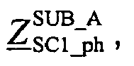
  - then an equivalent impedance of compensating bank at fault stage ${\underline{Z}}_{\mathrm{SC}1\mathrm{\_ph}}^{\mathrm{SUB\_A}}$
  
  nd ${\underline{Z}}_{\mathrm{SC}1\mathrm{\_ph}}^{\mathrm{SUB\_B}}$
  
  is calculated with using the post fault of measured voltage and currents and an equivalent impedance of compensation bank at pre-fault Z_{SC1_pre} is calculated in order to determine which distance d_A or d_B is the final result.
• Preferably the synchronization angle δ_A in term e^jδA is determined for phase-to-ground faults or phase-to-phase faults from the formula: $${\left[{\mathrm{e}}^{\mathrm{j}{\delta }_{\mathrm{A}}}\right]}_{\mathrm{ph}-\mathrm{g},\mathrm{ph}-\mathrm{ph}}=\frac{{\underline{a}}_{\mathrm{F}2}^{\mathrm{I}-\mathrm{SET}}{\underline{I}}_{\mathrm{SC}2\mathrm{\_B}}-{\underline{a}}_{\mathrm{F}1}^{\mathrm{II}-\mathrm{SET}}{\underline{I}}_{\mathrm{SC}1\mathrm{\_B}}}{{\underline{a}}_{\mathrm{F}1}^{\mathrm{II}-\mathrm{SET}}{\underline{\mathrm{N}}}_{\mathrm{A}1}-{\underline{a}}_{\mathrm{F}2}^{\mathrm{I}-\mathrm{SET}}{\underline{\mathrm{N}}}_{\mathrm{A}2}}$$

  

  
  where:
  subscript ph-g denotes phase to ground faults: a-g, b-g, c-g, and subscript ph-ph denotes phase to phase faults a-b, b-c, c-a,
  ${\underline{a}}_{\mathrm{F}2}^{\mathrm{I}-\mathrm{SET}},{\underline{a}}_{\mathrm{F}1}^{\mathrm{II}-\mathrm{SET}}-$

  

  denote the coefficients dependent on fault type,
  I _{SC1_B} - denotes the positive sequence current from the station B after analytical transfer towards series capacitor banks SC&MOV,
  I _{SC2_B} - denotes the negative sequence current from the station B after analytical transfer towards series capacitor banks SC&MOV,
  N _A1, N _A2 - denote the components dependent on positive and negative sequence currents and voltage taken at station A, respectively, as well as parameters of the line.
• Preferably the synchronization angle δ_A in term e^jδA s determined for the faults nor being the phase-to-ground faults or phase-to-phase faults from the formula: $${\mathrm{e}}^{\mathrm{j}{\mathrm{\delta }}_{\mathrm{A}}}=\frac{\left(1+{\underline{\mathrm{<figure-callout\; id="1"\; label="Z\; ̲"\; filenames="imgf0001.png,imgf0002.png"\; state="\{\{state\}\}">Z</figure-callout>}}}_{1\mathrm{B}}{\underline{\mathrm{<figure-callout\; id="1"\; label="Y\; ̲"\; filenames="imgf0001.png,imgf0002.png"\; state="\{\{state\}\}">Y</figure-callout>}}}_{1\mathrm{B}}\right)\left({\underline{\mathrm{<figure-callout\; id="1"\; label="Y\; ̲"\; filenames="imgf0001.png,imgf0002.png"\; state="\{\{state\}\}">Y</figure-callout>}}}_{1\mathrm{B}}{\underline{V}}_{\mathrm{B}1}^{\mathrm{pre}}-{\underline{I}}_{\mathrm{B}1}^{\mathrm{pre}}\right)+{\underline{\mathrm{<figure-callout\; id="1"\; label="Y\; ̲"\; filenames="imgf0001.png,imgf0002.png"\; state="\{\{state\}\}">Y</figure-callout>}}}_{1\mathrm{B}}{\underline{V}}_{\mathrm{B}1}^{\mathrm{pre}}}{\left(1+{\underline{\mathrm{<figure-callout\; id="1"\; label="Z\; ̲"\; filenames="imgf0001.png,imgf0002.png"\; state="\{\{state\}\}">Z</figure-callout>}}}_{1\mathrm{A}}{\underline{\mathrm{<figure-callout\; id="1"\; label="Y\; ̲"\; filenames="imgf0001.png,imgf0002.png"\; state="\{\{state\}\}">Y</figure-callout>}}}_{1\mathrm{A}}\right)\left({\underline{I}}_{\mathrm{A}1}^{\mathrm{pre}}-{\underline{\mathrm{<figure-callout\; id="1"\; label="Y\; ̲"\; filenames="imgf0001.png,imgf0002.png"\; state="\{\{state\}\}">Y</figure-callout>}}}_{1\mathrm{A}}{\underline{V}}_{\mathrm{A}1}^{\mathrm{pre}}\right)-{\underline{\mathrm{<figure-callout\; id="1"\; label="Y\; ̲"\; filenames="imgf0001.png,imgf0002.png"\; state="\{\{state\}\}">Y</figure-callout>}}}_{1\mathrm{A}}{\underline{V}}_{\mathrm{A}1}^{\mathrm{pre}}}$$

  

  
  where:
  ${\underline{V}}_{\mathrm{A}1}^{\mathrm{pre}},{\underline{V}}_{\mathrm{B}1}^{\mathrm{pre}}-$

  

  denote pre-fault positive sequence quantities (superscript 'pre' and subscript '1') of voltage measured at the ends A and B, respectively,
  ${\underline{I}}_{\mathrm{A}1}^{\mathrm{pre}},{\underline{I}}_{\mathrm{B}1}^{\mathrm{pre}}-$

  

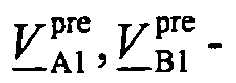
  denote pre-fault positive sequence quantities (superscript 'pre' and subscript '1') of current measured of the faulted line at the ends A and B, respectively,
  Z _1A, Y _1A - denote impedance and admittance of line section LA,
  Z _1B, Y ₁B - denote impedance and admittance of line section LB,
  LA - is the part of the line between line station A and series capacitor banks
  LB - is the part of the line between line station B and series capacitor banks
• Preferably the synchronization angle δ_B in term e^jδB is determined for phase-to-ground faults or phase-to-phase faults from the formula: $${\left[{\mathrm{e}}^{\mathrm{j}{\mathrm{\delta }}_{\mathrm{B}}}\right]}_{\mathrm{ph}-\mathrm{g},\mathrm{ph}-\mathrm{ph}}=\frac{{\underline{a}}_{\mathrm{F}2}^{\mathrm{I}-\mathrm{SET}}{\underline{I}}_{\mathrm{SC}2\mathrm{\_A}}-{\underline{a}}_{\mathrm{F}1}^{\mathrm{II}-\mathrm{SET}}{\underline{I}}_{\mathrm{SC}1\mathrm{\_A}}}{{\underline{a}}_{\mathrm{F}1}^{\mathrm{II}-\mathrm{SET}}{\underline{\mathrm{N}}}_{\mathrm{B}1}-{\underline{a}}_{\mathrm{F}2}^{\mathrm{I}-\mathrm{SET}}{\underline{\mathrm{N}}}_{\mathrm{B}2}}$$

  

  
  where:
  ${\underline{a}}_{\mathrm{F}2}^{\mathrm{I}-\mathrm{SET}},{\underline{a}}_{\mathrm{F}1}^{\mathrm{II}-\mathrm{SET}}-$

  

  denote the coefficients dependent of fault type,
  I _{SC1_A} - denotes positive sequence current from the station A after analytical transfer towards series capacitor banks SC&MOV,
  I _{SC2_A}- denotes negative sequence current from the station A after analytical transfer towards series capacitor banks SC&MOV ,
  N _B1, N _B2 - denote the components dependent on positive and negative sequence currents and voltage taken at station B, respectively, as well as parameters of the line.
• Preferably the synchronization angle (δ_B) in term e^jδB is determined for the faults nor being the phase-to-ground faults or phase-to-phase faults from the formula: $${\mathrm{e}}^{-\mathrm{j}{\mathrm{\delta }}_{\mathrm{B}}}=\frac{\left(1+{\underline{\mathrm{<figure-callout\; id="1"\; label="Z\; ̲"\; filenames="imgf0001.png,imgf0002.png"\; state="\{\{state\}\}">Z</figure-callout>}}}_{1\mathrm{B}}{\underline{\mathrm{<figure-callout\; id="1"\; label="Y\; ̲"\; filenames="imgf0001.png,imgf0002.png"\; state="\{\{state\}\}">Y</figure-callout>}}}_{1\mathrm{B}}\right)\left({\underline{\mathrm{<figure-callout\; id="1"\; label="Y\; ̲"\; filenames="imgf0001.png,imgf0002.png"\; state="\{\{state\}\}">Y</figure-callout>}}}_{1\mathrm{B}}{\underline{V}}_{\mathrm{B}1}^{\mathrm{pre}}-{\underline{I}}_{\mathrm{B}1}^{\mathrm{pre}}\right)+{\underline{\mathrm{<figure-callout\; id="1"\; label="Y\; ̲"\; filenames="imgf0001.png,imgf0002.png"\; state="\{\{state\}\}">Y</figure-callout>}}}_{1\mathrm{B}}{\underline{V}}_{\mathrm{B}1}^{\mathrm{pre}}}{\left(1+{\underline{\mathrm{<figure-callout\; id="1"\; label="Z\; ̲"\; filenames="imgf0001.png,imgf0002.png"\; state="\{\{state\}\}">Z</figure-callout>}}}_{1\mathrm{A}}{\underline{\mathrm{<figure-callout\; id="1"\; label="Y\; ̲"\; filenames="imgf0001.png,imgf0002.png"\; state="\{\{state\}\}">Y</figure-callout>}}}_{1\mathrm{A}}\right)\left({\underline{I}}_{\mathrm{A}1}^{\mathrm{pre}}-{\underline{\mathrm{<figure-callout\; id="1"\; label="Y\; ̲"\; filenames="imgf0001.png,imgf0002.png"\; state="\{\{state\}\}">Y</figure-callout>}}}_{1\mathrm{A}}{\underline{V}}_{\mathrm{A}1}^{\mathrm{pre}}\right)-{\underline{\mathrm{<figure-callout\; id="1"\; label="Y\; ̲"\; filenames="imgf0001.png,imgf0002.png"\; state="\{\{state\}\}">Y</figure-callout>}}}_{1\mathrm{A}}{\underline{V}}_{\mathrm{A}1}^{\mathrm{pre}}}$$

  

  
  where:
  ${\underline{V}}_{\mathrm{A}1}^{\mathrm{pre}},{\underline{V}}_{\mathrm{B}1}^{\mathrm{pre}}-$

  

  denote pre-fault positive sequence quantities (superscript 'pre' and subscript '1') of voltage measured at the ends A and B, respectively,
  ${\underline{I}}_{\mathrm{A}1}^{\mathrm{pre}},{\underline{I}}_{\mathrm{B}1}^{\mathrm{pre}}-$

  

  denote pre-fault positive sequence quantities (superscript 'pre' and subscript '1') of current measured of the faulted line at the ends A and B, respectively,
  Z _1A, Y ₁A - denote impedance and admittance of line section LA,
  Z _1B, Y _1B- denote impedance and admittance of line section LB,
  LA - is the part of the between line station A and series capacitor banks,
  LB - is the part of the between line station B and series capacitor banks.
• Preferably the distance to hypothetical fault d _LA is determined from the formula: $${\displaystyle \sum _{i=0}^2}{\underline{a}}_i\left({\underline{V}}_{\mathrm{A}i}\cosh \left({\underline{\mathrm{\gamma }}}_{i\mathrm{L}}{d}_{\mathrm{LA}}{\mathrm{p}}_{\mathrm{SC}}\ell \right)-{\underline{Z}}_{\mathrm{c}i\mathrm{L}}{\underline{I}}_{\mathrm{A}i}\sinh \left({\underline{\mathrm{\gamma }}}_{i\mathrm{L}}{d}_{\mathrm{LA}}{\mathrm{p}}_{\mathrm{SC}}\ell \right)\right)\cdot {\mathrm{e}}^{\mathrm{j}{\mathrm{\delta }}_{\mathrm{A}}}-R_{\mathrm{FA}}{\displaystyle \sum _{i=1}^2}\frac{{\underline{a}}_{\mathrm{F}i}{\underline{\mathrm{M}}}_i}{\cosh \left({\underline{\mathrm{\gamma }}}_{i\mathrm{L}}\left(1-d_{\mathrm{LA}}\right){\mathrm{p}}_{\mathrm{SC}}\ell \right)}=0$$

  

  
  for single line, $${\displaystyle \sum _{i=0}^2}{\underline{a}}_i\left({\underline{V}}_{\mathrm{A}i}\cosh \left({\underline{\mathrm{\gamma }}}_{i\mathrm{L}}{d}_{\mathrm{LA}}{\mathrm{p}}_{\mathrm{SC}}\ell \right)-{\underline{Z}}_{\mathrm{c}i\mathrm{L}}{\underline{I}}_{\mathrm{A}i}\sinh \left({\underline{\mathrm{\gamma }}}_{i\mathrm{L}}{d}_{\mathrm{LA}}{\mathrm{p}}_{\mathrm{SC}}\ell \right)\right)\cdot {\mathrm{e}}^{\mathrm{j}{\mathrm{\delta }}_{\mathrm{A}}}-R_{\mathrm{FA}}{\displaystyle \sum _{i=1}^2}\frac{{\underline{a}}_{\mathrm{F}i}{\underline{\mathrm{M}}}_i}{\cosh \left({\underline{\mathrm{\gamma }}}_{i\mathrm{L}}\left(1-d_{\mathrm{LA}}\right){\mathrm{p}}_{\mathrm{SC}}\ell \right)}-{\underline{a}}_{m0}{d}_{\mathit{LA}}{\mathrm{p}}_{\mathit{SC}}{\underline{Z}}_{0m}{\underline{I}}_{\mathrm{Aparal\_}0}\cdot {\mathrm{e}}^{\mathrm{j}{\mathrm{\delta }}_{\mathrm{A}}}=0$$

  

  
  for double- circuit line
  in which :
• d _LA - denotes the unknown distance to fault in [p.u.], expressed in relation to the length p_SCℓ of the line section between the station A and the series capacitor bank
• R _FA - denotes the unknown fault resistance,
• a ₁, a ₂, a ₀, a _m0- denotes the weighting coefficients dependent on fault type,
• M _i - denote numerical components for positive and negative sequences,
• Z _0m - mutual coupling impedance for zero sequence,
• I _{Aparal_0} - denotes zero sequence current from the station A measured in healthy parallel line,
• a _F1, a _F2 - denotes the share coefficients dependent on fault type.
• Preferably the distance to hypothetical fault d _LB is determined from the formula: $${\displaystyle \sum _{i=0}^2}{\underline{a}}_i\left({\underline{V}}_{\mathrm{B}i}\cosh \left({\underline{\mathit{\gamma }}}_{i\mathrm{L}}{d}_{\mathrm{LB}}\left(1-{\mathrm{p}}_{\mathrm{SC}}\right)\ell \right)-{\underline{Z}}_{\mathrm{c}i\mathrm{L}}{\underline{I}}_{\mathrm{B}i}\sinh \left({\underline{\mathit{\gamma }}}_{i\mathrm{L}}{d}_{\mathrm{LB}}{\mathrm{p}}_{\mathrm{SC}}\ell \right)\right)\cdot {\mathrm{e}}^{\mathrm{j}{\mathrm{\delta }}_{\mathrm{B}}}-R_{\mathrm{FB}}{\displaystyle \sum _{i=1}^2}\frac{{\underline{a}}_{\mathrm{F}i}{\underline{\mathrm{M}}}_i}{\cosh \left({\underline{\mathit{\gamma }}}_{i\mathrm{L}}\left(1-d_{\mathrm{LB}}\right)\left(1-{\mathrm{p}}_{\mathrm{SC}}\right)\ell \right)}=0$$

  

  
  for single line, $${\displaystyle \sum _{i=0}^2}{\underline{a}}_i\left({\underline{V}}_{\mathrm{B}i}\cosh \left({\underline{\mathrm{\gamma }}}_{i\mathrm{L}}{d}_{\mathrm{LB}}\left(1-{\mathrm{p}}_{\mathrm{SC}}\right)\ell \right)-{\underline{Z}}_{\mathrm{c}i\mathrm{L}}{\underline{I}}_{\mathrm{B}i}\sinh \left({\underline{\mathrm{\gamma }}}_{i\mathrm{L}}{d}_{\mathrm{LB}}\left(1-{\mathrm{p}}_{\mathrm{SC}}\right)\ell \right)\right)\cdot {\mathrm{e}}^{\mathrm{j}{\mathrm{\delta }}_{\mathrm{B}}}-R_{\mathrm{FB}}{\displaystyle \sum _{i=1}^2}\frac{{\underline{a}}_{\mathrm{F}i}{\underline{\mathrm{M}}}_i}{\cosh \left({\underline{\mathrm{\gamma }}}_{i\mathrm{L}}\left(1-d_{\mathrm{LB}}\right)\left(1-{\mathrm{p}}_{\mathrm{SC}}\right)\ell \right)}-{\underline{a}}_{m0}{d}_{\mathit{LB}}\left(1-{\mathrm{p}}_{\mathit{SC}}\right){\underline{Z}}_{0m}{\underline{I}}_{\mathrm{Bparal\_}0}\cdot {\mathrm{e}}^{\mathrm{j}{\mathrm{\delta }}_{\mathrm{B}}}=0$$

  

  
  for double-circuit line
  where:
• d _LB -denotes the unknown distance to fault in [p.u.], expressed in relation to the length (1-p_SC)ℓ of the line section between the station B and the series capacitor bank,
• R _FB - denotes the unknown fault resistance,
• M _i - denote numerical components for positive and negative sequences,
• a ₁, a ₂, a ₀, a _m0 - denotes the weighting coefficients dependent on fault type,
• a _F1, a _F2- denotes the share coefficients dependent on fault type,
• Z _0m - mutual coupling impedance for zero sequence,
• I _{Bparal_0} - denotes zero sequence current from the station B measured in parallel healthy line
• Preferably the final result d _A or d _B is chosen in the following steps
• first, it is check whether the fault resistances R _FA or R _FB are of positive value and if not, then such subroutine is rejected,
• next, the features of the estimated R-C equivalent circuit is checked and if it is satisfied the following dependence: $$\mathrm{real}\left({\underline{Z}}_{\mathrm{SC}1\mathrm{\_ph}}^{\mathrm{SUB\_A}}\right)>0,$$
  
  $$\mathrm{imag}\left({\underline{Z}}_{\mathrm{SC}1\mathrm{\_ph}}^{\mathrm{SUB\_A}}\right)<0,$$
  
  
  and imag $\left({\underline{Z}}_{\mathrm{SC}1\mathrm{\_ph}}^{\mathrm{SUB\_A}}\right)$
  
  > imag(Z _{SC1_pre})
  then that the fault has occurred between the station A and the SC&MOV bank, and the result d _A is a valid result,
  or if it is satisfied the following dependence:
  real $\left({\underline{Z}}_{\mathrm{SC}1\mathrm{\_ph}}^{\mathrm{SUB\_B}}\right)$
  
  >0,
  imag $\left({\underline{Z}}_{\mathrm{SC}1\mathrm{\_ph}}^{\mathrm{SUB\_B}}\right)$
  
  <0
  and imag $\left({\underline{Z}}_{\mathrm{SC}1\mathrm{\_ph}}^{\mathrm{SUB\_B}}\right)$
  
  > imag( Z _{SC1_pre}),
  then that the fault has occurred between the station B and the SC&MOV bank, and the result d _B is a valid result.
• A protection relay equipped with fault locator comprising means for performing the steps of at lest any of the claims 1 to 8.
• A computer program product comprising computer program code which when executed on a computing device caries out the steps of a method according to any of the claims 1 to 8.
• The advantage of the method according to the invention is the overcoming of all the limitations and drawbacks of the known methods that means that parameters and status of the series capacitor bank are not required to be known since they are not utilized for determination of the distance to fault and fault resistance, i.e. only the position at which the compensating banks are installed has to be known. Additionally the reactance of series capacitors is measured using the pre-fault measurements. The synchronization angle is determined using the pre-fault measurements or alternatively, for single phase-to-ground faults and phase-to-phase faults which are the most common faults with using the post-fault measurements, and with strict considering the distributed parameter line model, what allows accurate analytical synchronization of the measurements acquired asynchronously. Then, the distances to fault are calculated by introducing the compensation for shunt capacitances of the line with use of the distributed parameter line model. Selection of the valid subroutine is done based on multi-criteria procedure, what allows for reliable valid results identification within very wide range of fault conditions, even for very high fault resistances.
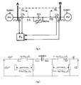
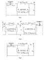
• The method according to the present invention is explained in an embodiment shown in the drawing, where fig.1 presents a general diagram of the electric network for the implementation of the inventive method , fig. 2 -an equivalent circuit diagram of series-compensated line for pre-fault positive sequence considered for determining the synchronization angle, fig. 3 - for fault FA an equivalent circuit diagram of series-compensated line for positive sequence - the part containing the SC&MOV and the section between the SC&MOV and the station B, fig. 4 - for fault FA an equivalent circuit diagram of series-compensated line for positive sequence - the part containing the SC&MOV and the section between the SC&MOV and the station A, fig. 5 - for fault FA an equivalent circuit diagram of series-compensated line for negative sequence - the part containing the SC&MOV and the section between the SC&MOV and the station B, fig.6 - for fault FA an equivalent circuit diagram of series-compensated line for negative sequence - the part containing the SC&MOV and the section between the SC&MOV and the station A, fig.7 - for fault FB an equivalent circuit diagram of series-compensated line for positive sequence - the part containing the SC&MOV and the section between the SC&MOV and the station A, fig.8 - for fault FB an equivalent circuit diagram of series-compensated line for positive sequence - the part containing the SC&MOV and the section between the SC&MOV and the station B, fig.9 - for fault FB an equivalent circuit diagram of series-compensated line for negative sequence - the part containing the SC&MOV and the section between the SC&MOV and the station A, fig.10 - for fault FB an equivalent circuit diagram of series-compensated line for negative sequence - the part containing the SC&MOV and the section between the SC&MOV and the station B, fig.11 - an equivalent circuit diagram of series -compensated line for the pre-fault positive sequence, considering for measuring the compensating bank impedance, fig.12 - a flow chart of the example of a fault location algorithm according to the present invention.
• The transmission system shown in fig. 1 consists of series compensated transmission line connecting two electric power stations A, and B. The installed series capacitor (SC-series capacitor) includes a metal oxide varistor (MOV- metal oxide varistor) connected in parallel (SC&MOV) which limits the voltage across the capacitor in a pre-defined manner. Station A is located at the beginning of the line, station B at the end of this line. In station A there is a fault locator FL. The fault locator can be also located at station B or at the separate place, what is not shown at the figure 1. Fault location is done using distributed parameters line model, models of faults and fault loops for symmetrical components positive, negative and zero, and different types of faults, by applying suitable share coefficients determining the relation between the symmetrical components of the total fault current when voltage drop across the fault resistance is estimated, defined as a _F1, a _F2, a _F0 and weight coefficients a ₁, a ₂, a ₀, a _m0 defining the share of individual components in the total model of the fault loop.
  Unsynchronised measurements of three-phase currents from stations A, B, and of three-phase voltages from station A and B are supplied to the fault locator FL. Fault locator is supplied with information about the type of the fault and the time of its occurrence. Then two hypothetical fault points are assumed and the distances d _A, and d _B between the beginning of the given line section A and B and the fault points (FA, FB) are calculated in order to determinate valid results, i.e. consistent with the real fault case, on the following assumptions:
• calculation of synchronization angle δ_A, the distance d _A from the beginning of the line in the station A to the fault point FA, fault resistance R _FA and impedance of compensation bank at faults state ${\underline{Z}}_{\mathrm{SC}1\mathrm{\_ph}}^{\mathrm{SUB\_A}},$
  
  impedance of compensation bank at pre-fault state Z_{SC1_pre}, assuming that the fault occurred in line section LA - steps 103a, 104a, 105a, 106a, where LA is the part of the line where the fault occurred between line station A and capacitor bank,
• calculation of synchronization angle δ_B, the distance d_B from the beginning of the line in the station B to the fault point FB, fault resistance R_FB and impedance of compensation bank at faults stage ${\underline{Z}}_{\mathrm{SC}1\mathrm{\_ph}}^{\mathrm{SUB\_B}},$
  
  impedance of compensation bank at pre-fault state Z _{SC1_pre}, assuming that the fault occurred in line section LB, where LB is the part of the line where the fault occurred between line station B and capacitor bank,- steps 103b, 104b, 105b, 106b.
Then among those two distances to fault d _A and d _B the valid results is selected - step 107.
• Step 101. In stations A and B, current and voltage input signals from individual phases for fault conditions I_{A_a}, I_{A_b}, I_{A_c}, V_{A_a}, V_{A_b}, V_{A_c}, I_{B_a}, I_{B_b}, I_{B_c}, V_{B_a}, V_{B_b}, V_{B_c} and for pre-fault conditions I_{A_pre_a}, I_{A_pre_b}, I_{A_pre-c}, V_{A_pre_a}, V_{A_pre_b}, V_{A_pre_c}, I_{B_pre_a}, I_{B_pre_b}, I_{B_pre_c}, V_{B_pre-a}, V_{B_pre_b}, V_{B_pre_c} and in case of double-circuit line currents from the healthy parallel line I_{Aparal_a}, I_{Apara_b}, I_{Aparal_c}, I_{Bparal_a}, I_{Bparal_b}, I_{Bparal_c} or only zero sequence currents I _{Aparal_0}, I _{Bparal_0} are measured.
• Step 102. In this step, the symmetrical components of the phase currents measured in stations A and B, and of phase voltages measured in stations A and B for pre-fault conditions and fault conditions are calculated. The details of such calculation are well known to those skilled in the art.
• Step 103a. In this step a synchronization angle δ_A is calculated as follows:
• if there are phase-to-ground faults or phase-to-phase faults then from the analyzing the total fault current flow fig.3, fig.4, fig.5, fig.6, based on the assumption that faults occurs in the line section between station A and series capacitor and metal oxide varistor device SC&MOV the synchronization angle δ_A in term e^jδA from the formula is determined: $${\left[{\mathrm{e}}^{\mathrm{j}{\delta }_{\mathrm{A}}}\right]}_{\mathrm{ph}-\mathrm{g},\mathrm{ph}-\mathrm{ph}}=\frac{{\underline{a}}_{\mathrm{F}2}^{\mathrm{I}-\mathrm{SET}}{\underline{I}}_{\mathrm{SC}2\mathrm{\_B}}-{\underline{a}}_{\mathrm{F}1}^{\mathrm{II}-\mathrm{SET}}{\underline{I}}_{\mathrm{SC}1\mathrm{\_B}}}{{\underline{a}}_{\mathrm{F}1}^{\mathrm{II}-\mathrm{SET}}{\underline{\mathrm{N}}}_{\mathrm{A}1}-{\underline{a}}_{\mathrm{F}2}^{\mathrm{I}-\mathrm{SET}}{\underline{\mathrm{N}}}_{\mathrm{A}2}}$$
  
where:
subscript ph-g denotes phase to ground faults: a-g, b-g, c-g, and subscript ph-ph denotes phase to phase faults a-b, b-c, c-a.
${\underline{a}}_{\mathrm{F}2}^{\mathrm{I}-\mathrm{SET}},{\underline{a}}_{\mathrm{F}1}^{\mathrm{II}-\mathrm{SET}}-$

denote the coefficients dependent of fault type gathered in Table 1, $${\underline{I}}_{\mathrm{SC}\mathrm{1}\mathrm{\_B}}=-\frac{1}{{\underline{Z}}_{\mathrm{c}\mathrm{1}\mathrm{L}}}\sinh \left({\underline{\mathit{\gamma }}}_{1\mathrm{L}}\left(1-{\mathrm{p}}_{\mathrm{SC}}\right)\ell \right)\cdot {\underline{V}}_{\mathrm{B}1}+\cosh \left({\underline{\mathit{\gamma }}}_{1\mathrm{L}}\left(1-{\mathrm{p}}_{\mathrm{SC}}\right)\ell \right)\cdot {\underline{I}}_{\mathrm{B}\mathrm{1}},$$


I _{SC1_B} - denotes the positive sequence current from the station B after analytical transfer towards series capacitor banks SC&MOV, $${\underline{I}}_{\mathrm{SC}\mathrm{2}\mathrm{\_B}}=-\frac{1}{{\underline{Z}}_{\mathrm{c}\mathrm{1}\mathrm{L}}}\sinh \left({\underline{\mathit{\gamma }}}_{1\mathrm{L}}\left(1-{\mathrm{p}}_{\mathrm{SC}}\right)\ell \right)\cdot {\underline{V}}_{\mathrm{B}2}+\cosh \left({\underline{\mathit{\gamma }}}_{1\mathrm{L}}\left(1-{\mathrm{p}}_{\mathrm{SC}}\right)\ell \right)\cdot {\underline{I}}_{\mathrm{B}\mathrm{1}},$$


I _{SC2_B} - denotes the negative sequence current from the station B after analytical transfer towards series capacitor banks SC&MOV, $${\underline{\mathrm{N}}}_{\mathrm{A}\mathrm{1}}=\cosh \left({\underline{\mathrm{\gamma }}}_{1\mathrm{L}}{\mathrm{p}}_{\mathrm{SC}}\ell \right)\cdot {\underline{I}}_{\mathrm{A}\mathrm{1}}-\frac{1}{{\underline{Z}}_{\mathrm{c}\mathrm{1}\mathrm{L}}}\sinh \left({\underline{\mathrm{\gamma }}}_{1\mathrm{L}}{\mathrm{p}}_{\mathrm{SC}}\ell \right)\cdot {\underline{V}}_{\mathrm{A}1},$$

$${\underline{\mathrm{N}}}_{\mathrm{A}2}=\cosh \left({\underline{\mathrm{\gamma }}}_{1\mathrm{L}}{\mathrm{p}}_{\mathrm{SC}}\ell \right)\cdot {\underline{I}}_{\mathrm{A}2}-\frac{1}{{\underline{Z}}_{\mathrm{c}\mathrm{1}\mathrm{L}}}\sinh \left({\underline{\mathrm{\gamma }}}_{1\mathrm{L}}{\mathrm{p}}_{\mathrm{SC}}\ell \right)\cdot {\underline{V}}_{\mathrm{A}2},$$


where:
• ℓ - denotes the total line length,
• p_SC - denotes the distance (p.u.) per unit length, at which the compensation bank (SC&MOV) is installed far away from the station A,
• ${\mathit{Z}}_{\mathrm{clL}=}\sqrt{\frac{{\underline{Z}}_{1\mathrm{L}}^{ʹ}}{{\underline{Y}}_{1\mathrm{L}}^{ʹ}}}-$
  
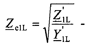
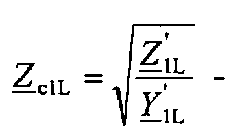
  denotes the characteristic impedance of the line for the positive sequence,
• ${\mathrm{<figure-callout\; id="1"\; label="\gamma "\; filenames="imgf0001.png,imgf0002.png"\; state="\{\{state\}\}">\gamma </figure-callout>}}_{1\mathrm{L}=}\sqrt{{\underline{Z}}_{1\mathrm{L}}^{ʹ}{\underline{Y}}_{1\mathrm{L}}^{ʹ}}-$
  
  denotes the propagation constant of the line for the positive sequence,
• Z '_1L, Y '_1L - denote the positive sequence impedance and admittance of the line per unit length.
It was considered for determining the negative-sequence quantities according to equations (3) and (5) that the positive- and negative-sequence line parameters are identical, as in reality. For both sequences the line parameters for the positive sequence (subscript: 1) are used. This is also applied in the following considerations.
• Analysis of boundary conditions for different types of faults shows that there is a certain degree of freedom when determining the share coefficients determining the relation between the symmetrical components of the total fault current when voltage drop across the fault resistance is estimated. Their selection depends on the adopted preference of the use of individual sequence components depending on the type of the fault. In the presented example of the invention embodiment, in order to ensure high precision of the fault location, voltage drop across the fault resistance is estimated using positive and negative sequence components.
• There are two characteristic alternative sets (among the other possible) of the share coefficients for the phase-to-ground a-g, b-g, c-g, and phase-to-phase faults a-b, b-c, c-a, as gathered in the table 1. Table 1. Phase-to-ground faults and phase-to-phase faults - two alternative sets of share coefficients.

  FAULT	I-SET		II-SET
  	${\underline{\mathrm{a}}}_{\mathrm{F}\mathrm{1}}$	${\underline{\mathrm{a}}}_{\mathrm{F}2}$	${\underline{\mathrm{a}}}_{\mathrm{F}\mathrm{1}}$	${\underline{\mathrm{a}}}_{\mathrm{F}2}$
  a-g	0	3	3	0
  b-g	0	3a	3a 2	0
  c-g	0	3a 2	3a	0
  a-b	0	1-a	1-a 2	0
  b-c	0	a-a 2	a 2-a	0
  c-a	0	a 2-1	a-1	0
  a=exp(j2π/3)

• In contrast to the above fault types, the other situation is for the remaining fault types (phase-to-phase-to-ground and three phase symmetrical faults). This is so, since for these remaining faults there is no alternative sets of the share coefficients for the positive and the negative sequence - as gathered in the table 2. Table 2. Set of share coefficients for phase-to-phase-to-ground faults and three phase faults.

  FAULT	a F1	a F2
  a-b-g, a-b-c,	1-a 2	1-a
  a-b-c-g
  b-c-g	a 2-a	a-a 2
  c-a-g	a-1	a 2-1

• The type of the fault is denoted by symbols: a-g, b-g, c-g , a-b, b-c, c-a, a-b-g, a-b-c, a-b-c-g, b-c-g, c-a-g, where letters a, b, c denote individual phases, and letter g denotes earthing (ground), index 1 denotes the positive-sequence component, index 2 - the negative component.
• If there are not a phase-to-ground faults and not phase-to-phase faults, then the synchronization angle δ_A in term e^jδA from the analysis of the current flow for the pre-fault conditions (fig.2) with using the distributed parameter line model is calculated from the formula: $${\mathrm{e}}^{\mathrm{j}{\mathrm{\delta }}_{\mathrm{A}}}=\frac{\left(1+{\underline{Z}}_{1\mathrm{B}}{\underline{Y}}_{1\mathrm{B}}\right)\left({\underline{Y}}_{1\mathrm{B}}{\underline{V}}_{\mathrm{B}1}^{\mathrm{pre}}-{\underline{I}}_{\mathrm{B}1}^{\mathrm{pre}}\right)+{\underline{Y}}_{1\mathrm{B}}{\underline{V}}_{\mathrm{B}1}^{\mathrm{<figure-callout\; id="1"\; label="pre"\; filenames="imgf0001.png,imgf0002.png"\; state="\{\{state\}\}">pre</figure-callout>}}}{\left(1+{\underline{Z}}_{1\mathrm{A}}{\underline{Y}}_{1\mathrm{A}}\right)\left({\underline{I}}_{\mathrm{A}1}^{\mathrm{pre}}-{\underline{Y}}_{1\mathrm{A}}{\underline{V}}_{\mathrm{A}1}^{\mathrm{pre}}\right)-{\underline{Y}}_{1\mathrm{A}}{\underline{V}}_{\mathrm{A}1}^{\mathrm{pre}}}$$

  

  
  where:
• Z _1A = ${\mathrm{p}}_{\mathrm{SC}}\ell {\underline{A}}_{1\mathrm{sh\_p}}{\underline{Z}}_{1\mathrm{L}}^{ʹ},$
  
• ${\underline{Y}}_{1\mathrm{A}}=0.5{\mathrm{p}}_{\mathrm{SC}}\ell {\underline{A}}_{1\mathrm{th\_p}}{\underline{Y}}_{1\mathrm{L}}^{ʹ},$
  
• ${\underline{Z}}_{1\mathrm{B}}=\left(1-{\mathrm{p}}_{\mathrm{SC}}\right)\ell {\underline{A}}_{1\mathrm{th\_}1-\mathrm{p}}{\underline{Z}}_{1\mathrm{L}}^{ʹ},$
  
• Y _1B = $0.5\left(1-{\mathrm{p}}_{\mathrm{SC}}\right)\ell {\underline{A}}_{1\mathrm{th\_}1-\mathrm{p}}{\underline{Y}}_{1\mathrm{L}}^{ʹ},$
  
  $${\underline{A}}_{1\mathrm{sh\_p}}=\frac{\sinh \left({\underline{\mathit{\gamma }}}_{1\mathrm{L}}{\mathrm{p}}_{\mathrm{SC}}\ell \right)}{{\underline{\mathit{\gamma }}}_{1\mathrm{L}}{\mathrm{p}}_{\mathrm{SC}}\ell },$$
  
  $${\underline{A}}_{1\mathrm{sh\_p}}=\frac{\tanh \left(0.5{\underline{\mathit{\gamma }}}_{1\mathrm{L}}{\mathrm{p}}_{\mathrm{SC}}\ell \right)}{0.5{\underline{\mathit{\gamma }}}_{1\mathrm{L}}{\mathrm{p}}_{\mathrm{SC}}\ell },$$
  
  $${\underline{A}}_{1\mathrm{sh\_}\mathrm{1}-\mathrm{p}}=\frac{\sinh \left({\underline{\mathit{\gamma }}}_{1\mathrm{L}}\left(1-{\mathrm{p}}_{\mathrm{SC}}\right)\ell \right)}{{\underline{\mathit{\gamma }}}_{1\mathrm{L}}\left(1-{\mathrm{p}}_{\mathrm{SC}}\right)\ell },$$
  
  $${\underline{A}}_{1\mathrm{th\_}\mathrm{1}-\mathrm{p}}=\frac{\tanh \left(0.5{\underline{\mathit{\gamma }}}_{1\mathrm{L}}\left(1-{\mathrm{p}}_{\mathrm{SC}}\right)\ell \right)}{0.5{\underline{\mathit{\gamma }}}_{1\mathrm{L}}\left(1-{\mathrm{p}}_{\mathrm{SC}}\right)\ell },$$
  
• ${\underline{V}}_{\mathrm{A}1}^{\mathrm{pre}},{\underline{V}}_{\mathrm{B}1}^{\mathrm{pre}}-$
  
  denote pre-fault positive sequence quantities (superscript 'pre' and subscript '1') of voltage measured at the ends A and B, respectively,
• denote pre-fault positive sequence quantities (superscript 'pre' and subscript '1') of current measured of the faulted line at the ends A and B, respectively.
• Step 104a. Having determined the synchronization angle δ_A, and in consequence the synchronization operator e^jδA, one multiplies the phasors of the signals from the station A by this operator. This assures common reference for the phasors of signals acquired asynchronously at both line ends.
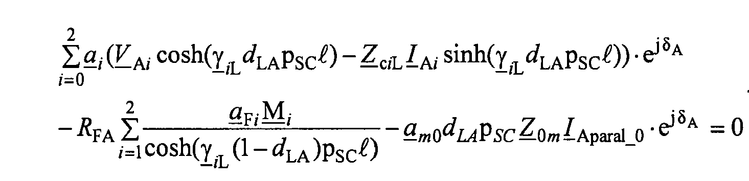
  Taking into account the distributed parameter line model, the following generalised fault loop model is applied, covering different fault types, what is reflected with use of the appropriate weighting coefficients: a _j and share coefficients: a _Fi , both dependent on a fault type, where i=0,1,2 and denote i-th symmetrical component, where the a ₁, a ₂, a ₀, a _m0 - weighting coefficients gathered in the table 3 and a _F1, a _F2 - share coefficients gathered in the table 4. $${\displaystyle \sum _{i=0}^2}{\underline{a}}_i\left({\underline{V}}_{\mathrm{A}i}\cosh \left({\underline{\mathrm{\gamma }}}_{i\mathrm{L}}{d}_{\mathrm{LA}}{\mathrm{p}}_{\mathrm{SC}}\ell \right)-{\underline{Z}}_{\mathrm{c}i\mathrm{L}}{\underline{I}}_{\mathrm{A}i}\sinh \left({\underline{\mathrm{\gamma }}}_{i\mathrm{L}}{d}_{\mathrm{LA}}{\mathrm{p}}_{\mathrm{SC}}\ell \right)\right)\cdot {\mathrm{e}}^{\mathrm{j}{\mathrm{\delta }}_{\mathrm{A}}}-R_{\mathrm{FA}}{\displaystyle \sum _{i=1}^2}\frac{{\underline{a}}_{\mathrm{F}i}{\underline{\mathrm{M}}}_i}{\cosh \left({\underline{\mathrm{\gamma }}}_{i\mathrm{L}}\left(1-d_{\mathrm{LA}}\right){\mathrm{p}}_{\mathrm{SC}}\ell \right)}=0$$

  

  
  for single line, $${\displaystyle \sum _{i=0}^2}{\underline{a}}_i\left({\underline{V}}_{\mathrm{A}i}\cosh \left({\underline{\mathrm{\gamma }}}_{i\mathrm{L}}{d}_{\mathrm{LA}}{\mathrm{p}}_{\mathrm{SC}}\ell \right)-{\underline{Z}}_{\mathrm{c}i\mathrm{L}}{\underline{I}}_{\mathrm{A}i}\sinh \left({\underline{\mathrm{\gamma }}}_{i\mathrm{L}}{d}_{\mathrm{LA}}{\mathrm{p}}_{\mathrm{SC}}\ell \right)\right)\cdot {\mathrm{e}}^{\mathrm{j}{\mathrm{\delta }}_{\mathrm{A}}}-R_{\mathrm{FA}}{\displaystyle \sum _{i=1}^2}\frac{{\underline{a}}_{\mathrm{F}i}{\underline{\mathrm{M}}}_i}{\cosh \left({\underline{\mathrm{\gamma }}}_{i\mathrm{L}}\left(1-d_{\mathrm{LA}}\right){\mathrm{p}}_{\mathrm{SC}}\ell \right)}-{\underline{a}}_{m0}{d}_{\mathit{LA}}{\mathrm{p}}_{\mathit{SC}}{\underline{Z}}_{0m}{\underline{I}}_{\mathrm{Aparal\_}0}\cdot {\mathrm{e}}^{\mathrm{j}{\mathrm{\delta }}_{\mathrm{A}}}=0$$

  

  
  for double- circuit line
  where:
• d _LA - denotes the unknown hypothetical distance to fault in [p.u.], expressed in relation to the length (p_SCℓ) of the line section between the station A and the series capacitor bank,
• R_FA - denotes the unknown fault resistance, $${\underline{\mathrm{M}}}_{\mathrm{1}}=\cosh \left({\underline{\mathit{\gamma }}}_{1\mathrm{L}}{\mathrm{p}}_{\mathrm{SC}}\ell \right){\underline{I}}_{\mathrm{A}\mathrm{1}}{\mathrm{e}}^{\mathrm{j}{\mathrm{\delta }}_{\mathrm{A}}}-\frac{\sinh \left({\underline{\mathit{\gamma }}}_{1\mathrm{L}}{\mathrm{p}}_{\mathrm{SC}}\ell \right){\underline{V}}_{\mathrm{A}1}{\mathrm{e}}^{\mathrm{j}{\mathrm{\delta }}_{\mathrm{A}}}}{{\underline{Z}}_{\mathrm{c}\mathrm{1}\mathrm{L}}}-\frac{\sinh \left({\underline{\mathit{\gamma }}}_{1\mathrm{L}}\left(1-{\mathrm{p}}_{\mathrm{SC}}\right)\ell \right)\cdot {\underline{V}}_{\mathrm{B}1}}{{\underline{Z}}_{\mathrm{c}\mathrm{1}\mathrm{L}}}+\cosh \left({\underline{\mathit{\gamma }}}_{1\mathrm{L}}\left(1-{\mathrm{p}}_{\mathrm{SC}}\right)\ell \right)\cdot {\underline{I}}_{\mathrm{B}\mathrm{1}},$$
  
  $${\underline{\mathrm{M}}}_2=\cosh \left({\underline{\mathit{\gamma }}}_{1\mathrm{L}}{\mathrm{p}}_{\mathrm{SC}}\ell \right){\underline{I}}_{\mathrm{A}2}{\mathrm{e}}^{\mathrm{j}{\mathrm{\delta }}_{\mathrm{A}}}-\frac{\sinh \left({\underline{\mathit{\gamma }}}_{1\mathrm{L}}{\mathrm{p}}_{\mathrm{SC}}\ell \right){\underline{V}}_{\mathrm{A}2}{\mathrm{e}}^{\mathrm{j}{\mathrm{\delta }}_{\mathrm{A}}}}{{\underline{Z}}_{\mathrm{c}\mathrm{1}\mathrm{L}}}-\frac{\sinh \left({\underline{\mathit{\gamma }}}_{1\mathrm{L}}\left(1-{\mathrm{p}}_{\mathrm{SC}}\right)\ell \right)\cdot {\underline{V}}_{\mathrm{B}2}}{{\underline{Z}}_{\mathrm{c}\mathrm{1}\mathrm{L}}}+\cosh \left({\underline{\mathit{\gamma }}}_{1\mathrm{L}}\left(1-{\mathrm{p}}_{\mathrm{SC}}\right)\ell \right)\cdot {\underline{I}}_{\mathrm{B}2},$$
  
• a ₁, a ₂, a ₀, a _m0- denote the weighting coefficients dependent on fault type gathered in the table 3,
• a _F1, a _F2 - denote the share coefficients dependent on fault type gathered in the table 4,
• Z _0m - mutual coupling impedance for zero sequence,
• I _{Aparal_0} - denotes zero sequence current from the station A measured in healthy parallel line
Table 3. Weighting Coefficients for Composing Fault loop Voltage And Current

FAULT	a 1	a 2	a 0	a m0
a-g	1	1	1	1
b-g	$\mathrm{0.5}\mathrm{-}\mathrm{j}\mathrm{0.5}\sqrt{\mathrm{3}}$	$\mathrm{0.5}+\mathrm{j}\mathrm{0.5}\sqrt{\mathrm{3}}$	1	1
c-g	$\mathrm{0.5}+\mathrm{j}\mathrm{0.5}\sqrt{\mathrm{3}}$	$-\mathrm{0.5}\mathrm{-}\mathrm{j}\mathrm{0.5}\sqrt{\mathrm{3}}$	1	1
a-b, a-b-g	$\mathrm{1.5}+\mathrm{j}\mathrm{0.5}\sqrt{\mathrm{3}}$	$\mathrm{1.5}\mathrm{-}\mathrm{j}\mathrm{0.5}\sqrt{\mathrm{3}}$	0	0
a-b-c, a-b-c-g
b-c, b-c-g	$\mathrm{-}\mathrm{j}\sqrt{\mathrm{3}}$	$\mathrm{j}\sqrt{\mathrm{3}}$	0	0
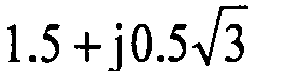
c-a, c-a-g	-1.5 + j	$-\mathrm{1.5}\mathrm{-}\mathrm{j}\mathrm{0.5}\sqrt{\mathrm{3}}$	0	0
a 0m - used in case of double circuit lines for mutual coupling compensation

Table 4. Share Coefficients Used For calculation Of Total Fault Current

FAULT	a F1	a F2	a F0
a-g	0	3	0
b-g	0	$\mathrm{1.5}+\mathrm{j}\mathrm{1.5}\sqrt{\mathrm{3}}$	0
c-g	0	$-\mathrm{1.5}-\mathrm{j}\mathrm{1.5}\sqrt{\mathrm{3}}$	0
a-b	0	$\mathrm{1.5}-\mathrm{j}\mathrm{0.5}\sqrt{\mathrm{3}}$	0
b-c	0	$\mathrm{j}\sqrt{\mathrm{3}}$	0
c-a	0	$-\mathrm{1.5}-\mathrm{j}\mathrm{0.5}\sqrt{\mathrm{3}}$	0
a-b-g	$\mathrm{1.5}+\mathrm{j}\mathrm{0.5}\sqrt{\mathrm{3}}$	$\mathrm{1.5}-\mathrm{j}\mathrm{0.5}\sqrt{\mathrm{3}}$	0
b-c-g	$-\mathrm{j}\sqrt{\mathrm{3}}$	$\mathrm{j}\sqrt{\mathrm{3}}$	0
c-a-g	$-\mathrm{1.5}+\mathrm{j}\mathrm{0.5}\sqrt{\mathrm{3}}$	$-\mathrm{1.5}-\mathrm{j}\mathrm{0.5}\sqrt{\mathrm{3}}$	0
a-b-c	$\mathrm{1.5}+\mathrm{j}\mathrm{0.5}\sqrt{\mathrm{3}}$	$\mathrm{1.5}-\mathrm{j}\mathrm{0.5}{\sqrt{\mathrm{3}}}^{*)}$	0
a-b-c-g
j = $\sqrt{-1},$ *) - a F2 ≠ 0, however the negative sequence components are not present in the signals

• Resolving equation (7) or (8) into the real / imaginary parts allows to solve it for the unknowns: d _LA and R _FA. As for example, the iterative Newton-Raphson method can be applied for that. This method requires setting the starting values for the sought values. These values can be set to: 0.5 [p.u.] for d _LA and 0 for R _FA.
• After completing the solution of (7) or (8), the distance to fault d _A [p.u.], which is related to the whole line length ℓ, between the stations A and B, is calculated as: $$d_{\mathrm{A}}={\mathrm{p}}_{\mathrm{SC}}{d}_{\mathrm{LA}}$$

  

  
  where d _LA is the result from the last iterative solution of the equation (7) or (8).
• Step 105a. In this step the equivalent impedance of compensating bank at fault stage is calculated with using the post fault values of measured voltage and currents. $${\underline{Z}}_{\mathrm{SC}1\mathrm{\_ph}}^{\mathrm{SUB\_A}}=\frac{\mathrm{\Delta }{\underline{V}}_{\mathrm{SC\_ph}}^{\mathrm{SUB\_A}}}{{\underline{I}}_{\mathrm{SC\_ph}}^{\mathrm{SUB\_A}}}$$

  

  
  where: $$\mathrm{\Delta }{\underline{V}}_{\mathrm{SC\_ph}}^{\mathrm{SUB\_A}}={\underline{a}}_{1\_}\Delta {\underline{V}}_{\mathrm{<figure-callout\; id="1"\; label="SC\_"\; filenames="imgf0001.png,imgf0002.png"\; state="\{\{state\}\}">SC\_</figure-callout>}1}^{\mathrm{SUB\_A}}+{\underline{a}}_{2\_}\Delta {\underline{V}}_{\mathrm{<figure-callout\; id="2"\; label="SC\_"\; filenames="imgf0001.png"\; state="\{\{state\}\}">SC\_</figure-callout>}2}^{\mathrm{SUB\_A}}+{\underline{a}}_{0\_}\mathrm{\Delta }{\underline{V}}_{\mathrm{SC\_}0}^{\mathrm{SUB\_A}},$$

  

  $${\underline{I}}_{\mathrm{SC\_ph}}^{\mathrm{SUB\_A}}={\underline{a}}_{1\_}\Delta {\underline{I}}_{\mathrm{SC\_}1}^{\mathrm{SUB\_A}}+{\underline{a}}_{2\_}\Delta {\underline{I}}_{\mathrm{SC\_}2}^{\mathrm{SUB\_A}}+{\underline{a}}_{0\_}{\underline{I}}_{\mathrm{SC\_}0}^{\mathrm{SUB\_A}},$$

  
• $\mathrm{\Delta }{\underline{V}}_{\mathrm{SC\_ph}}^{\mathrm{SUB\_A}},{\underline{I}}_{\mathrm{SC\_ph}}^{\mathrm{SUB\_A}}-$

  

  denote the phase quantities of voltage and currents calculated from i-th symmetrical components of voltage drop and i-th symmetrical component of current entering SC&MOV bank, with neglecting the shunt capacitances of the line:
• in case of single phase to ground fault: the faulted phase
• in case of inter-phase fault: any of the faulted phases, $\mathrm{\Delta }{\underline{V}}_{\mathrm{SC\_}i}^{\mathrm{SUB\_A}}={\underline{V}}_{\mathrm{B}i}-{\underline{V}}_{\mathrm{A}i}{\mathrm{e}}^{\mathrm{j}{\mathrm{\delta }}_{\mathrm{A}}}-Z_{i\mathrm{L}}{I}_{\mathrm{B}i}+d_{\mathrm{A}}\left({\underline{Z}}_{i\mathrm{L}}{\underline{I}}_{\mathrm{A}i}{\mathrm{e}}^{\mathrm{j}{\mathrm{\delta }}_{\mathrm{A}}}+Z_{i\mathrm{L}}{I}_{\mathrm{B}i}\right)-$
  
  denotes the i-th symmetrical component of voltage drop across the SCs&MOVs, ${\underline{I}}_{\mathrm{SC\_}i}^{\mathrm{SUB\_A}}$
  
  = I _Bi - denotes i-th symmetrical component of current entering SC&MOV bank, with neglecting the shunt capacitances of the line, a _{1_}, a _{2_} , a _{0_} - complex coefficients dependent on fault type which are selected in such a way that in case of:
• single phase to ground fault - the faulted phase, as for example for a-g fault the equivalent impedance of SC&MOV in phase 'a' is determined,
• inter-phase fault - any of the faulted phases, as for example for a-b fault the equivalent impedance of SC&MOV in phase 'a' is determined.
• Step 106a. At this stage the equivalent impedance of compensation bank at pre-fault stage is calculated: $${\underline{Z}}_{\mathrm{SC}1\mathrm{\_pre}}=\frac{\mathrm{\Delta }{\underline{V}}_{\mathrm{SC}1}^{\mathrm{pre}}}{{\underline{I}}_{\mathrm{SC}1\mathrm{\_B}}^{\mathrm{pre}}}$$

  

  
  where: $$\mathrm{\Delta }{\underline{V}}_{\mathrm{SC}1}^{\mathrm{pre}}={\underline{V}}_{\mathrm{SC}1\mathrm{\_B}}^{\mathrm{pre}}-{\underline{V}}_{\mathrm{SC}1\mathrm{\_A}}^{\mathrm{pre}}{\mathrm{e}}^{\mathrm{j}{\mathrm{\delta }}_{\mathrm{A}}},$$

  

  $${\underline{V}}_{\mathrm{SC}1\mathrm{\_A}}^{\mathrm{pre}}=\cosh \left({\underline{\mathit{\gamma }}}_{1\mathrm{L}}{\mathrm{p}}_{\mathrm{SC}}\ell \right)\cdot {\underline{V}}_{\mathrm{A}1}^{\mathrm{pre}}-{\underline{Z}}_{\mathrm{c}\mathrm{1}\mathrm{L}}\sinh \left({\underline{\mathit{\gamma }}}_{1\mathrm{L}}{\mathrm{p}}_{\mathrm{SC}}\ell \right)\cdot {\underline{I}}_{\mathrm{A}1}^{\mathrm{pre}},$$

  

  $${\underline{V}}_{\mathrm{SC}1\mathrm{\_B}}^{\mathrm{pre}}=\cosh \left({\underline{\mathrm{\gamma }}}_{1\mathrm{L}}\left(1-{\mathrm{p}}_{\mathrm{SC}}\right)\ell \right)\cdot {\underline{V}}_{\mathrm{B}1}^{\mathrm{pre}}-{\underline{Z}}_{\mathrm{c}\mathrm{1}\mathrm{L}}\sinh \left({\underline{\mathrm{\gamma }}}_{1\mathrm{L}}\left(1-{\mathrm{p}}_{\mathrm{SC}}\right)\ell \right)\cdot {\underline{I}}_{\mathrm{B}1}^{\mathrm{pre}},$$

  

  $${\underline{I}}_{\mathrm{SC}1\mathrm{\_B}}^{\mathrm{pre}}=-\frac{1}{{\underline{Z}}_{\mathrm{c}\mathrm{1}\mathrm{L}}}\sinh \left({\underline{\mathrm{\gamma }}}_{1\mathrm{L}}\left(1-{\mathrm{p}}_{\mathrm{SC}}\right)\ell \right)\cdot {\underline{V}}_{\mathrm{B}1}^{\mathrm{pre}}+\cosh \left({\underline{\mathrm{\gamma }}}_{1\mathrm{L}}\left(1-{\mathrm{p}}_{\mathrm{SC}}\right)\ell \right)\cdot {\underline{I}}_{\mathrm{B}1}^{\mathrm{pre}}\mathrm{.}$$

  
• Step 103b. In this step the synchronization angle is calculated as follows: if there is phase-to-ground faults or phase-to-phase faults then from the analyzing the total fault current flow (fig.7, fig.8, fig.9, fig.10), based on the assumption that faults occurs in the line section between station B and series capacitor and metal oxide varistor device SC&MOV determining the synchronization angle δ_B in term e^jδB from the formula: $${\left[{\mathrm{e}}^{\mathrm{j}{\mathrm{\delta }}_{\mathrm{B}}}\right]}_{\mathrm{ph}-\mathrm{g},\mathrm{ph}-\mathrm{ph}}=\frac{{\underline{a}}_{\mathrm{F}2}^{\mathrm{I}-\mathrm{SET}}{\underline{I}}_{\mathrm{SC}2\mathrm{\_A}}-{\underline{a}}_{\mathrm{F}1}^{\mathrm{II}-\mathrm{SET}}{\underline{I}}_{\mathrm{SC}1\mathrm{\_A}}}{{\underline{a}}_{\mathrm{F}1}^{\mathrm{II}-\mathrm{SET}}{\underline{\mathrm{N}}}_{\mathrm{B}1}-{\underline{a}}_{\mathrm{F}2}^{\mathrm{I}-\mathrm{SET}}{\underline{\mathrm{N}}}_{\mathrm{B}2}}$$

  

  
  where:
  ${\underline{a}}_{\mathrm{F}2}^{\mathrm{I}-\mathrm{SET}},{\underline{a}}_{\mathrm{F}1}^{\mathrm{II}-\mathrm{SET}}-$

  

  denote the coefficients dependent of fault type gathered in table 1, $${\underline{I}}_{\mathrm{SC}\mathrm{1}\mathrm{\_A}}=-\frac{1}{{\underline{Z}}_{\mathrm{c}\mathrm{1}\mathrm{L}}}\sinh \left({\underline{\mathit{\gamma }}}_{1\mathrm{L}}{\mathrm{p}}_{\mathrm{SC}}\ell \right)\cdot {\underline{V}}_{\mathrm{A}1}+\cosh \left({\underline{\mathit{\gamma }}}_{1\mathrm{L}}{\mathrm{p}}_{\mathrm{SC}}\ell \right)\cdot {\underline{I}}_{\mathrm{A}\mathrm{1}},$$

  

  
  I _{SC1_A}- denotes positive sequence current from the station A after analytical transfer towards series capacitor banks SC&MOV, $${\underline{I}}_{\mathrm{SC}\mathrm{2}\mathrm{\_A}}=-\frac{1}{{\underline{Z}}_{\mathrm{c}\mathrm{1}\mathrm{L}}}\sinh \left({\underline{\mathit{\gamma }}}_{1\mathrm{L}}{\mathrm{p}}_{\mathrm{SC}}\ell \right)\cdot {\underline{V}}_{\mathrm{A}2}+\cosh \left({\underline{\mathit{\gamma }}}_{1\mathrm{L}}{\mathrm{p}}_{\mathrm{SC}}\ell \right)\cdot {\underline{I}}_{\mathrm{A}2},$$

  

  
  I _{SC2_A}- denotes negative sequence current from the station A after analytical transfer towards series capacitor banks SC&MOV , $${\underline{\mathrm{N}}}_{\mathrm{B}\mathrm{1}}=\cosh \left({\underline{\mathit{\gamma }}}_{1\mathrm{L}}\left(1-{\mathrm{p}}_{\mathrm{SC}}\right)\ell \right)\cdot {\underline{I}}_{\mathrm{B}\mathrm{1}}-\frac{1}{{\underline{Z}}_{\mathrm{c}\mathrm{1}\mathrm{L}}}\sinh \left({\underline{\mathit{\gamma }}}_{1\mathrm{L}}\left(1-{\mathrm{p}}_{\mathrm{SC}}\right)\ell \right)\cdot {\underline{V}}_{\mathrm{B}1},$$

  

  $${\underline{\mathrm{N}}}_{\mathrm{B}2}=\cosh \left({\underline{\mathit{\gamma }}}_{1\mathrm{L}}\left(1-{\mathrm{p}}_{\mathrm{SC}}\right)\ell \right)\cdot {\underline{I}}_{\mathrm{B}2}-\frac{1}{{\underline{Z}}_{\mathrm{c}\mathrm{1}\mathrm{L}}}\sinh \left({\underline{\mathit{\gamma }}}_{1\mathrm{L}}\left(1-{\mathrm{p}}_{\mathrm{SC}}\right)\ell \right)\cdot {\underline{V}}_{\mathrm{B}2},$$

  

  
  where:
  ℓ - denotes total line length,
  p_SC - denotes distance (p.u.) at which the compensation bank (SCs&MOVs) is installed far away from the station A,
  ${\mathrm{Z}}_{\mathrm{ciL}}=\sqrt{\frac{{\underline{Z}}_{1\mathrm{L}}^{ʹ}}{{\underline{Y}}_{1\mathrm{L}}^{ʹ}}}-$

  

  denotes characteristic impedance of the line for the positive sequence,
  ${\mathit{<figure-callout\; id="1"\; label="\gamma "\; filenames="imgf0001.png,imgf0002.png"\; state="\{\{state\}\}">\gamma </figure-callout>}}_{1\mathrm{L}}=\sqrt{{\underline{Z}}_{1\mathrm{L}}^{ʹ}{\underline{Y}}_{1\mathrm{L}}^{ʹ}}-$

  

  denotes propagation constant of the line for the positive sequence,
  ${\underline{Z}}_{1\mathrm{L}}^{ʹ},{\underline{Y}}_{1\mathrm{L}}^{ʹ}-$

  

  denote positive sequence impedance and admittance of the line per unit length.
  It was considered for determining the negative-sequence quantities according to equations (14) and (16) that the positive- and negative-sequence line parameters are identical, as in reality. For both sequences the line parameters for the positive sequence (subscript: 1) are used. This is also applied in the following considerations:
• if there are not phase-to-ground faults and not phase-to-phase faults then determining the synchronization angle δ_B for phase-to-ground faults and phase-to-phase faults in term e^jδB from the formula (6).
• Step 104b . Having determined the synchronization angle δ_B, and in consequence the synchronization operator e^jδB , one multiplies the phasors of the signals from the end B by this operator. This assures common reference for the phasors of signals acquired asynchronously at both line ends.
  Taking into account the distributed parameter line model, the following generalised fault loop model, covering different fault types, what is reflected with use of the appropriate weighting coefficients: a _i and share coefficients: a _Fi , both dependent on a fault type is applied, where the a ₁, a ₂, a ₀ a _m0- weighting coefficients gathered in the table 3 and a _F1, a _F2 - share coefficients gathered in the table 4. $${\displaystyle \sum _{i=0}^2}{\underline{a}}_i\left({\underline{V}}_{\mathrm{B}i}\cosh \left({\underline{\mathit{\gamma }}}_{i\mathrm{L}}{d}_{\mathrm{LB}}\left(1-{\mathrm{p}}_{\mathrm{SC}}\right)\ell \right)-{\underline{Z}}_{\mathrm{c}i\mathrm{L}}{\underline{I}}_{\mathrm{B}i}\sinh \left({\underline{\mathit{\gamma }}}_{i\mathrm{L}}{d}_{\mathrm{LB}}\left(1-{\mathrm{p}}_{\mathrm{SC}}\right)\ell \right)\right)\cdot {\mathrm{e}}^{\mathrm{j}{\mathrm{\delta }}_{\mathrm{B}}}-R_{\mathrm{FB}}{\displaystyle \sum _{i=1}^2}\frac{{\underline{a}}_{\mathrm{F}i}{\underline{\mathrm{M}}}_i}{\cosh \left({\underline{\mathit{\gamma }}}_{i\mathrm{L}}\left(1-d_{\mathrm{LB}}\right)\left(1-{\mathrm{p}}_{\mathrm{SC}}\right)\ell \right)}=0$$

  

  
  for single line, $${\displaystyle \sum _{i=0}^2}{\underline{a}}_i\left({\underline{V}}_{\mathrm{B}i}\cosh \left({\underline{\mathrm{\gamma }}}_{i\mathrm{L}}{d}_{\mathrm{LB}}\left(1-{\mathrm{p}}_{\mathrm{SC}}\right)\ell \right)-{\underline{Z}}_{\mathrm{c}i\mathrm{L}}{\underline{I}}_{\mathrm{B}i}\sinh \left({\underline{\mathrm{\gamma }}}_{i\mathrm{L}}{d}_{\mathrm{LB}}\left(1-{\mathrm{p}}_{\mathrm{SC}}\right)\ell \right)\right)\cdot {\mathrm{e}}^{\mathrm{j}{\mathrm{\delta }}_{\mathrm{B}}}-R_{\mathrm{FB}}{\displaystyle \sum _{i=1}^2}\frac{{\underline{a}}_{\mathrm{F}i}{\underline{\mathrm{M}}}_i}{\cosh \left({\underline{\mathrm{\gamma }}}_{i\mathrm{L}}\left(1-d_{\mathrm{LB}}\right)\left(1-{\mathrm{p}}_{\mathrm{SC}}\right)\ell \right)}-{\underline{a}}_{m0}{d}_{\mathit{LB}}\left(1-{\mathrm{p}}_{\mathit{SC}}\right){\underline{Z}}_{0m}{\underline{I}}_{\mathrm{Bparal\_}0}\cdot {\mathrm{e}}^{\mathrm{j}{\mathrm{\delta }}_{\mathrm{B}}}=0$$

  

  
  for double-circuit line
  where:
• d _LB -denotes the unknown hiphotetical distance to fault in [p.u.], expressed in relation to the length ((1-p_SC)ℓ) of the line section between the station B and the series capacitor bank,
• R _FB - denotes the unknown fault resistance, $${\underline{\mathrm{M}}}_{\mathrm{1}}=\cosh \left({\underline{\mathit{\gamma }}}_{1\mathrm{L}}\left(1-{\mathrm{p}}_{\mathrm{SC}}\right)\ell \right){\underline{I}}_{\mathrm{B}\mathrm{1}}{\mathrm{e}}^{\mathrm{j}{\mathrm{\delta }}_{\mathrm{B}}}-\frac{\sinh \left({\underline{\mathit{\gamma }}}_{1\mathrm{L}}\left(1-{\mathrm{p}}_{\mathrm{SC}}\right)\ell \right){\underline{V}}_{\mathrm{B}1}{\mathrm{e}}^{\mathrm{j}{\mathrm{\delta }}_{\mathrm{B}}}}{{\underline{Z}}_{\mathrm{c}\mathrm{1}\mathrm{L}}}-\frac{\sinh \left({\underline{\mathit{\gamma }}}_{1\mathrm{L}}{\mathrm{p}}_{\mathrm{SC}}\ell \right)\cdot {\underline{V}}_{\mathrm{A}1}}{{\underline{Z}}_{\mathrm{c}\mathrm{1}\mathrm{L}}}+\cosh \left({\underline{\mathit{\gamma }}}_{1\mathrm{L}}{\mathrm{p}}_{\mathrm{SC}}\ell \right)\cdot {\underline{I}}_{\mathrm{A}\mathrm{1}},$$
  
  $${\underline{\mathrm{M}}}_2=\cosh \left({\underline{\mathit{\gamma }}}_{1\mathrm{L}}\left(1-{\mathrm{p}}_{\mathrm{SC}}\right)\ell \right){\underline{I}}_{\mathrm{B}2}{\mathrm{e}}^{\mathrm{j}{\mathrm{\delta }}_{\mathrm{B}}}-\frac{\sinh \left({\underline{\mathit{\gamma }}}_{1\mathrm{L}}\left(1-{\mathrm{p}}_{\mathrm{SC}}\right)\ell \right){\underline{V}}_{\mathrm{B}2}{\mathrm{e}}^{\mathrm{j}{\mathrm{\delta }}_{\mathrm{B}}}}{{\underline{Z}}_{\mathrm{c}\mathrm{1}\mathrm{L}}}-\frac{\sinh \left({\underline{\mathit{\gamma }}}_{1\mathrm{L}}{\mathrm{p}}_{\mathrm{SC}}\ell \right)\cdot {\underline{V}}_{\mathrm{A}2}}{{\underline{Z}}_{\mathrm{c}\mathrm{1}\mathrm{L}}}+\cosh \left({\underline{\mathit{\gamma }}}_{1\mathrm{L}}{\mathrm{p}}_{\mathrm{SC}}\ell \right)\cdot {\underline{I}}_{\mathrm{A}2},$$
  
• a ₁, a ₂, a ₀, a _m0 - denote weighting coefficients dependent on fault type gathered in table 3,
• a _F1, a _F2 - denote share coefficients dependent on fault type, gathered in table 4,
• Z _0m - mutual coupling impedance for zero sequence,
• I _{Bparal_0}- denotes zero sequence current from the station B measured in parallel line
• Resolving equation (17) or (18) into the real / imaginary parts allows to solve it for the unknowns: d _LB, R _FB. As for example, the iterative Newton-Raphson method can be applied for that. This method requires setting the starting values for the sought values. These values can be set to: 0.5 [p.u.] for d _LB and 0 for R _FB.
• After completing the solution of (17) or (18), the distance to fault d _B [p.u.], which is related to the whole line length ℓ, between the stations A and B, is calculated as: $$d_{\mathrm{B}}=\left(1-{\mathrm{p}}_{\mathrm{SC}}\right)d_{\mathrm{LB}}$$

  

  
  where d _LB is the result from the last iterative solution of (17) or (18).
• Step 105B. The equivalent impedance of compensating bank at fault stage is calculated with using the post fault values of measured voltage and currents: $${\underline{Z}}_{\mathrm{SC}1\mathrm{\_ph}}^{\mathrm{SUB\_B}}=\frac{\mathrm{\Delta }{\underline{V}}_{\mathrm{SC\_ph}}^{\mathrm{SUB\_B}}}{{\underline{I}}_{\mathrm{SC\_ph}}^{\mathrm{SUB\_B}}}$$

  

  
  where: $$\mathrm{\Delta }{\underline{V}}_{\mathrm{SC\_ph}}^{\mathrm{SUB\_B}}={\underline{a}}_{1\_}\Delta {\underline{V}}_{\mathrm{<figure-callout\; id="1"\; label="SC\_"\; filenames="imgf0001.png,imgf0002.png"\; state="\{\{state\}\}">SC\_</figure-callout>}1}^{\mathrm{SUB\_B}}+{\underline{a}}_{2\_}\Delta {\underline{V}}_{\mathrm{<figure-callout\; id="2"\; label="SC\_"\; filenames="imgf0001.png"\; state="\{\{state\}\}">SC\_</figure-callout>}2}^{\mathrm{SUB\_B}}+{\underline{a}}_{0\_}\mathrm{\Delta }{\underline{V}}_{\mathrm{SC\_}0}^{\mathrm{SUB\_B}},$$

  

  $${\underline{I}}_{\mathrm{SC\_ph}}^{\mathrm{SUB\_B}}={\underline{a}}_{1\_}\Delta {\underline{I}}_{\mathrm{SC\_}1}^{\mathrm{SUB\_B}}+{\underline{a}}_{2\_}\Delta {\underline{I}}_{\mathrm{SC\_}2}^{\mathrm{SUB\_B}}+{\underline{a}}_{0\_}{\underline{I}}_{\mathrm{SC\_}0}^{\mathrm{SUB\_B}},$$

  
• $\mathrm{\Delta }{\underline{V}}_{\mathrm{SC\_ph}}^{\mathrm{SUB\_B}},{\underline{I}}_{\mathrm{SC\_ph}}^{\mathrm{SUB\_A}}-$

  

  denote phase quantities of voltage and currents calculated from i-th symmetrical components of voltage drop and i-th symmetrical component of current entering SC&MOV bank, with neglecting the shunt capacitances of the line
• in case of single phase to ground fault: the faulted phase,
• in case of inter-phase fault : any of the faulted phases,
  a _{1_}, a _{2_}, a _{0_} - denote complex coefficients dependent on fault type, which are selected in such a way that in case of:
• single phase to ground fault: the faulted phase, as for example for a-g fault the equivalent impedance of SC&MOV in phase 'a' is determined,
• inter-phase fault : any of the faulted phases, as for example for a-b fault the equivalent impedance of SC&MOV in phase 'a' is determined,
$\mathrm{\Delta }{\underline{V}}_{\mathrm{SC\_}i}^{\mathrm{SUB\_B}}={\underline{V}}_{\mathrm{A}i}-{\underline{V}}_{\mathrm{B}i}{\mathrm{e}}^{\mathrm{j}{\mathrm{\delta }}_{\mathrm{B}}}-Z_{i\mathrm{L}}{I}_{\mathrm{B}i}+d_{\mathrm{B}}\left({\underline{Z}}_{i\mathrm{L}}{\underline{I}}_{\mathrm{A}i}+Z_{i\mathrm{L}}{I}_{\mathrm{B}i}{\mathrm{e}}^{\mathrm{j}{\mathrm{\delta }}_{\mathrm{B}}}\right)-$

denotes the voltage drop across the SCs&MOVs for the i-th symmetrical component,
${\underline{I}}_{\mathrm{SC\_}i}^{\mathrm{SUB\_B}}$

= I _Ai - denote the i-th symmetrical component of current entering SC&MOV bank, with neglecting the shunt capacitances of the line.
• Step 106b. At this stage the equivalent impedance of compensation bank at pre-fault stage is calculated as in step 106a
• Step 107. At this step the selection of final results is generated.
  First, it is check whether the particular subroutine I and subroutine II yields the distance to fault within the section range and whether the fault resistance is of positive value. If this is not, so (if the determined distance to fault lays outside the section range and/or the fault resistance is negative) then such subroutine is rejected.
  Next, the features of the estimated R-C equivalent circuit are checked.
  If it is satisfied the following dependence: $$\mathrm{real}\left({\underline{Z}}_{\mathrm{SC}1\mathrm{\_ph}}^{\mathrm{SUB\_A}}\right)>0,$$

  

  $$\mathrm{imag}\left({\underline{Z}}_{\mathrm{SC}1\mathrm{\_ph}}^{\mathrm{SUB\_A}}\right)<0$$

  

  
  and $$\mathrm{imag}\left({\underline{Z}}_{\mathrm{SC}1\mathrm{\_ph}}^{\mathrm{SUB\_A}}\right)>\mathrm{imag}\left({\underline{Z}}_{\mathrm{SC}1\mathrm{\_pre}}^{ʹ}\right)$$

  

  
  that denotes, that the fault has occurred between the station A and the SC&MOV bank, and the results:
  d_A - distance to fault (p.u.), counted from the station A up to fault point F(fig.1),
  R_FA - fault resistance,
  are the valid results, i.e. consistent with the real fault case.
• If opposite dependences are satisfying, that means : $$\mathrm{real}\left({\underline{Z}}_{\mathrm{SC}1\mathrm{\_ph}}^{\mathrm{SUB\_B}}\right)>0,$$

  

  $$\mathrm{imag}\left({\underline{Z}}_{\mathrm{SC}1\mathrm{\_ph}}^{\mathrm{SUB\_B}}\right)<0$$

  

  
  and $$\mathrm{imag}\left({\underline{Z}}_{\mathrm{SC}1\mathrm{\_ph}}^{\mathrm{SUB\_B}}\right)>\mathrm{imag}\left({\underline{Z}}_{\mathrm{SC}1\mathrm{\_pre}}\right),$$

  

  
  that denotes that the fault has occurred between the station B and the SC&MOV bank, and the results:
  d_B - distance to fault (p.u.), counted from the station B up to fault point F (fig.1), R_FB - fault resistance,
  are the valid results, i.e. consistent with the real fault case.

Claims (10)

1. A method for fault location in series compensated power transmission lines with two- end unsynchronized measurement wherein a distance to fault and fault resistance are determined by means of voltages and currents values, measurement in the stations (A) and (B), before and after occurrence of the fault, characterizes in that:

   - based on the assumption that fault occurs in the line section LA between station A and series capacitor and metal oxide varistor device SC&MOV and based on the assumption that faults occurs in the line section LB between station B and series capacitor and metal oxide varistor device SC&MOV, the synchronization angle δ_A in term e^jδA is determined in the first case (fault at the section LA), the synchronization angle δ_B in term e^jδB is determined in the second case (fault at the section LB).,

   - then taking into account the distributed parameter line model the distance to fault (d _A) or (d _B) is determined from the formula: $$d_{\mathrm{A}}={\mathrm{p}}_{\mathrm{SC}}{d}_{\mathrm{LA}},$$

   

   $$d_{\mathrm{B}}=\left(1-{\mathrm{p}}_{\mathrm{SC}}\right)d_{\mathrm{LB}}$$

   

   where:

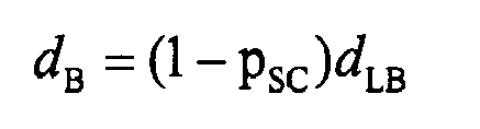   d _LA, d _LB - denotes an hypothetical distance to fault, expressed in relation to length p_SCℓ and (1-p_SC)ℓ, respectively, and which value is received by solving the fault loop formula using known iterative method,

   - then an equivalent impedance of compensating bank at fault stage $\left({\underline{Z}}_{\mathrm{SC}1\mathrm{\_ph}}^{\mathrm{SUB\_A}}\right)$

   

   and $\left({\underline{Z}}_{\mathrm{SC}1\mathrm{\_ph}}^{\mathrm{SUB\_B}}\right)$

   

   is calculated with using the post fault of measured voltage and currents and an equivalent impedance of compensation bank at pre-fault (Z_{SC1_pre}) is calculated in order to determine which distance (d _A) or (d _B) is the final result.
2. A method according to claim 1, characterised in that the synchronization angle (δ_A) in term e^jδA is determined for phase-to-ground faults or phase-to-phase faults from the formula: $${\left[{\mathrm{e}}^{\mathrm{j}{\delta }_{\mathrm{A}}}\right]}_{\mathrm{ph}-\mathrm{g},\mathrm{ph}-\mathrm{ph}}=\frac{{\underline{a}}_{\mathrm{F}2}^{\mathrm{I}-\mathrm{SET}}{\underline{I}}_{\mathrm{SC}2\mathrm{\_B}}-{\underline{a}}_{\mathrm{F}1}^{\mathrm{II}-\mathrm{SET}}{\underline{I}}_{\mathrm{SC}1\mathrm{\_B}}}{{\underline{a}}_{\mathrm{F}1}^{\mathrm{II}-\mathrm{SET}}{\underline{\mathrm{N}}}_{\mathrm{A}1}-{\underline{a}}_{\mathrm{F}2}^{\mathrm{I}-\mathrm{SET}}{\underline{\mathrm{N}}}_{\mathrm{A}2}}$$

   

   
   where:

   subscript ph-g denotes phase to ground faults: a-g, b-g, c-g, and subscript ph-ph denotes phase to phase faults a-b, b-c, c-a,

   ${\underline{a}}_{\mathrm{F}2}^{\mathrm{I}-\mathrm{SET}},{\underline{a}}_{\mathrm{F}1}^{\mathrm{II}-\mathrm{SET}}-$

   

   denote the coefficients dependent on fault type,

   I _{SC1_B} - denotes the positive sequence current from the station B after analytical transfer towards series capacitor banks SC&MOV,
   I _{SC2_B} - denotes the negative sequence current from the station B after analytical transfer towards series capacitor banks SC&MOV,
   N _A1, N _A2 - denote the coefficients dependent on positive and negative sequence currents and voltage taken at station A respectively as well as parameters of the line.
3. A method according to claim 1, characterised in that the synchronization angle (δ_A) in term e^jδA is determined for the faults nor being the phase-to-ground faults or phase-to-phase faults from the formula: $${\mathrm{e}}^{\mathrm{j}{\mathrm{\delta }}_{\mathrm{A}}}=\frac{\left(1+{\underline{Z}}_{1\mathrm{B}}{\underline{Y}}_{1\mathrm{B}}\right)\left({\underline{Y}}_{1\mathrm{B}}{\underline{V}}_{\mathrm{B}1}^{\mathrm{pre}}-{\underline{I}}_{\mathrm{B}1}^{\mathrm{pre}}\right)+{\underline{Y}}_{1\mathrm{B}}{\underline{V}}_{\mathrm{B}1}^{\mathrm{pre}}}{\left(1+{\underline{Z}}_{1\mathrm{A}}{\underline{Y}}_{1\mathrm{A}}\right)\left({\underline{I}}_{\mathrm{A}1}^{\mathrm{pre}}-{\underline{Y}}_{1\mathrm{A}}{\underline{V}}_{\mathrm{A}1}^{\mathrm{pre}}\right)-{\underline{Y}}_{1\mathrm{A}}{\underline{V}}_{\mathrm{A}1}^{\mathrm{pre}}}$$

   

   
   where:

   ${\underline{V}}_{\mathrm{A}1}^{\mathrm{pre}},{\underline{V}}_{\mathrm{B}1}^{\mathrm{pre}}-$

   

   denote pre-fault positive sequence quantities (superscript 'pre' and subscript '1') of voltage measured at the ends A and B, respectively,

   ${\underline{I}}_{\mathrm{A}1}^{\mathrm{pre}},{\underline{I}}_{\mathrm{B}1}^{\mathrm{pre}}-$

   

   denote pre-fault positive sequence quantities (superscript 'pre' and subscript '1') of current measured of the faulted line at the ends A and B, respectively,

   Z _1A, Y _1A - denote impedance and admittance of line section LA,

   Z _1B, Y ₁B - denote impedance and admittance of line section LB,

   LA - is the part of the line between line station A and series capacitor banks

   LB - is the part of the line between line station B and series capacitor banks.
4. A method according to claim 1, characterised in that the synchronization angle (δ_B) in term e^jδB is determined for phase-to-ground faults or phase-to-phase faults from the formula: $${\left[{\mathrm{e}}^{\mathrm{j}{\mathrm{\delta }}_{\mathrm{B}}}\right]}_{\mathrm{ph}-\mathrm{g},\mathrm{ph}-\mathrm{ph}}=\frac{{\underline{a}}_{\mathrm{F}2}^{\mathrm{I}-\mathrm{SET}}{\underline{I}}_{\mathrm{SC}2\mathrm{\_A}}-{\underline{a}}_{\mathrm{F}1}^{\mathrm{II}-\mathrm{SET}}{\underline{I}}_{\mathrm{SC}1\mathrm{\_A}}}{{\underline{a}}_{\mathrm{F}1}^{\mathrm{II}-\mathrm{SET}}{\underline{\mathrm{N}}}_{\mathrm{B}1}-{\underline{a}}_{\mathrm{F}2}^{\mathrm{I}-\mathrm{SET}}{\underline{\mathrm{N}}}_{\mathrm{B}2}}$$

   

   
   where:

   ${\underline{a}}_{\mathrm{F}2}^{\mathrm{I}-\mathrm{SET}},{\underline{a}}_{\mathrm{F}1}^{\mathrm{II}-\mathrm{SET}}-$

   

   denote the coefficients dependent of fault type,

   I _{SC1_A} - denotes positive sequence current from the station A after analytical transfer towards series capacitor banks SC&MOV,

   I _{SC2_A}- denotes negative sequence current from the station A after analytical transfer towards series capacitor banks SC&MOV ,

   N _B1, N _B2 - denote the coefficients dependent on positive and negative sequence currents and voltage taken at station B respectively as well as parameters of the line.
5. A method according to claim 1, characterised in that the synchronization angle (δ_B) in term e^jδB is determined for the faults nor being the phase-to-ground faults or phase-to-phase faults from the formula: $${\mathrm{e}}^{-\mathrm{j}{\mathrm{\delta }}_{\mathrm{B}}}=\frac{\left(1+{\underline{Z}}_{1\mathrm{B}}{\underline{Y}}_{1\mathrm{B}}\right)\left({\underline{Y}}_{1\mathrm{B}}{\underline{V}}_{\mathrm{B}1}^{\mathrm{pre}}-{\underline{I}}_{\mathrm{B}1}^{\mathrm{pre}}\right)+{\underline{Y}}_{1\mathrm{B}}{\underline{V}}_{\mathrm{B}1}^{\mathrm{pre}}}{\left(1+{\underline{Z}}_{1\mathrm{A}}{\underline{Y}}_{1\mathrm{A}}\right)\left({\underline{I}}_{\mathrm{A}1}^{\mathrm{pre}}-{\underline{Y}}_{1\mathrm{A}}{\underline{V}}_{\mathrm{A}1}^{\mathrm{pre}}\right)-{\underline{Y}}_{1\mathrm{A}}{\underline{V}}_{\mathrm{A}1}^{\mathrm{pre}}}$$

   

   
   where:

   ${\underline{V}}_{\mathrm{A}1}^{\mathrm{pre}},{\underline{V}}_{\mathrm{B}1}^{\mathrm{pre}}-$

   

   denote pre-fault positive sequence quantities (superscript 'pre' and subscript '1') of voltage measured at the ends A and B, respectively,

   ${\underline{I}}_{\mathrm{A}1}^{\mathrm{pre}},{\underline{I}}_{\mathrm{B}1}^{\mathrm{pre}}-$

   

   denote pre-fault positive sequence quantities (superscript 'pre' and subscript '1') of current measured of the faulted line at the ends A and B, respectively,

   Z _1A, Y _1A - denote impedance and admittance of line section LA,

   Z _1B, Y _1B- denote impedance and admittance of line section LB.

   LA - is the part of the line between line station A and series capacitor banks

   LB - is the part of the between line station B and series capacitor banks.
6. A method according to claim 1, characterised in that the distance to hypothetical fault (d _LA) is determined from the formula: $${\displaystyle \sum _{i=0}^2}{\underline{a}}_i\left({\underline{V}}_{\mathrm{A}i}\cosh \left({\underline{\mathrm{\gamma }}}_{i\mathrm{L}}{d}_{\mathrm{LA}}{\mathrm{p}}_{\mathrm{SC}}\ell \right)-{\underline{Z}}_{\mathrm{c}i\mathrm{L}}{\underline{I}}_{\mathrm{A}i}\sinh \left({\underline{\mathrm{\gamma }}}_{i\mathrm{L}}{d}_{\mathrm{LA}}{\mathrm{p}}_{\mathrm{SC}}\ell \right)\right)\cdot {\mathrm{e}}^{\mathrm{j}{\mathrm{\delta }}_{\mathrm{A}}}-R_{\mathrm{FA}}{\displaystyle \sum _{i=1}^2}\frac{{\underline{a}}_{\mathrm{F}i}{\underline{\mathrm{M}}}_i}{\cosh \left({\underline{\mathrm{\gamma }}}_{i\mathrm{L}}\left(1-d_{\mathrm{LA}}\right){\mathrm{p}}_{\mathrm{SC}}\ell \right)}=0$$

   

   
   for single line, $${\displaystyle \sum _{i=0}^2}{\underline{a}}_i\left({\underline{V}}_{\mathrm{A}i}\cosh \left({\underline{\mathrm{\gamma }}}_{i\mathrm{L}}{d}_{\mathrm{LA}}{\mathrm{p}}_{\mathrm{SC}}\ell \right)-{\underline{Z}}_{\mathrm{c}i\mathrm{L}}{\underline{I}}_{\mathrm{A}i}\sinh \left({\underline{\mathrm{\gamma }}}_{i\mathrm{L}}{d}_{\mathrm{LA}}{\mathrm{p}}_{\mathrm{SC}}\ell \right)\right)\cdot {\mathrm{e}}^{\mathrm{j}{\mathrm{\delta }}_{\mathrm{A}}}-R_{\mathrm{FA}}{\displaystyle \sum _{i=1}^2}\frac{{\underline{a}}_{\mathrm{F}i}{\underline{\mathrm{M}}}_i}{\cosh \left({\underline{\mathrm{\gamma }}}_{i\mathrm{L}}\left(1-d_{\mathrm{LA}}\right){\mathrm{p}}_{\mathrm{SC}}\ell \right)}-{\underline{a}}_{m0}{d}_{\mathit{LA}}{\mathrm{p}}_{\mathit{SC}}{\underline{Z}}_{0m}{\underline{I}}_{\mathrm{Aparal\_}0}\cdot {\mathrm{e}}^{\mathrm{j}{\mathrm{\delta }}_{\mathrm{A}}}=0$$

   

   
   for double- circuit line
   in which :

   R_FA - denotes the unknown fault resistance,

   a ₁, a ₂, a ₀, a _m0 - denotes the weighting coefficients dependent on fault type,

   M _i - denote numerical components for positive and negative sequences,

   a _F1, a _F2 - denotes the share coefficients dependent on fault type,

   Z _0m - mutual coupling impedance for zero sequence,

   I _{Aparal_0} - denotes zero sequence current from the station A measured in healthy parallel line.
7. A method according to claim 1, characterised in that the distance to hypothetical fault (d_LB) is determined from the formula: $${\displaystyle \sum _{i=0}^2}{\underline{a}}_i\left({\underline{V}}_{\mathrm{B}i}\cosh \left({\underline{\mathit{\gamma }}}_{i\mathrm{L}}{d}_{\mathrm{LB}}\left(1-{\mathrm{p}}_{\mathrm{SC}}\right)\ell \right)-{\underline{Z}}_{\mathrm{c}i\mathrm{L}}{\underline{I}}_{\mathrm{B}i}\sinh \left({\underline{\mathit{\gamma }}}_{i\mathrm{L}}{d}_{\mathrm{LB}}\left(1-{\mathrm{p}}_{\mathrm{SC}}\right)\ell \right)\right)\cdot {\mathrm{e}}^{\mathrm{j}{\mathrm{\delta }}_{\mathrm{B}}}-R_{\mathrm{FB}}{\displaystyle \sum _{i=1}^2}\frac{{\underline{a}}_{\mathrm{F}i}{\underline{\mathrm{M}}}_i}{\cosh \left({\underline{\mathit{\gamma }}}_{i\mathrm{L}}\left(1-d_{\mathrm{LB}}\right)\left(1-{\mathrm{p}}_{\mathrm{SC}}\right)\ell \right)}=0$$

   

   
   for single line, $${\displaystyle \sum _{i=0}^2}{\underline{a}}_i\left({\underline{V}}_{\mathrm{B}i}\cosh \left({\underline{\mathit{\gamma }}}_{i\mathrm{L}}{d}_{\mathrm{LB}}\left(1-{\mathrm{p}}_{\mathrm{SC}}\right)\ell \right)-{\underline{Z}}_{\mathrm{c}i\mathrm{L}}{\underline{I}}_{\mathrm{B}i}\sinh \left({\underline{\mathit{\gamma }}}_{i\mathrm{L}}{d}_{\mathrm{LB}}\left(1-{\mathrm{p}}_{\mathrm{SC}}\right)\ell \right)\right)\cdot {\mathrm{e}}^{\mathrm{j}{\mathrm{\delta }}_{\mathrm{B}}}$$

   

   $$-R_{\mathrm{FB}}{\displaystyle \sum _{i=1}^2}\frac{{\underline{a}}_{\mathrm{F}i}{\underline{\mathrm{M}}}_i}{\cosh \left({\underline{\mathit{\gamma }}}_{i\mathrm{L}}\left(1-d_{\mathrm{LB}}\right)\left(1-{\mathrm{p}}_{\mathrm{SC}}\right)\ell \right)}-{\underline{a}}_{m0}{d}_{\mathit{LB}}\left(1-{\mathrm{p}}_{\mathit{SC}}\right){\underline{Z}}_{0m}{\underline{I}}_{\mathrm{Bparal\_}0}\cdot {\mathrm{e}}^{\mathrm{j}{\mathrm{\delta }}_{\mathrm{B}}}=0$$

   

   
   for double-circuit line
   where:

   d _LB -denotes the unknown distance to fault in [p.u.], expressed in relation to the length ((1-p_SC)ℓ) of the line section between the station B and the series capacitor bank,

   R _FB - denotes the unknown fault resistance,

   M _i - denote numerical coefficients for positive and negative sequences,

   a ₁, a ₂, a ₀, a _{m 0} - denotes the weighting coefficients dependent on fault type,

   a _F1, a _F2 - denotes the share coefficients dependent on fault type.

   Z _0m - mutual coupling impedance for zero sequence,

   I _{Bparal_0} - denotes zero sequence current from the station B measured in healthy parallel line
8. The method according any previous claims, characterized in that the final result (d _A) or (d _B) is chosen in the following steps

   - first, it is check whether the fault resistances (R _FA) or (R _FB) are of positive value and if not, then such subroutine is rejected,

   - next, the features of the estimated R-C equivalent circuit are checked and if it is satisfied the following dependence: $$\mathrm{real}\left({\underline{Z}}_{\mathrm{SC}1\mathrm{\_ph}}^{\mathrm{SUB\_A}}\right)>0,$$

   

   $$\mathrm{imag}\left({\underline{Z}}_{\mathrm{SC}1\mathrm{\_ph}}^{\mathrm{SUB\_A}}\right)<0,$$

   

   
   and $$\mathrm{imag}\left({\underline{Z}}_{\mathrm{SC}1\mathrm{\_ph}}^{\mathrm{SUB\_A}}\right)>\mathrm{imag}\left({\underline{Z}}_{\mathrm{SC}1\mathrm{\_pre}}\right)$$

   

   
   then that the fault has occurred between the station A and the SC&MOV bank, and the result (d _A) is a valid result,
   or if it is satisfied the following dependence: $$\mathrm{real}\left({\underline{Z}}_{\mathrm{SC}1\mathrm{\_ph}}^{\mathrm{SUB\_B}}\right)>0,$$

   

   $$\mathrm{imag}\left({\underline{Z}}_{\mathrm{SC}1\mathrm{\_ph}}^{\mathrm{SUB\_B}}\right)<0$$

   

   
   and $$\mathrm{imag}\left({\underline{Z}}_{\mathrm{SC}1\mathrm{\_ph}}^{\mathrm{SUB\_B}}\right)>\mathrm{imag}\left({\underline{Z}}_{\mathrm{SC}1\mathrm{\_pre}}\right),$$

   

   
   then that the fault has occurred between the station B and the SC&MOV bank, and the result (d_B) is a valid result.
9. A protection relay equipped with fault locator (FL) comprising means for performing the steps of at lest any of the claims 1 to 8.
10. A computer program product comprising computer program code which when executed on a computing device caries out the steps of a method according to any of the claims 1 to 8.

Images