EP1701005A1 - Method and apparatus for the calculation of energy and technical processes - Google Patents
Method and apparatus for the calculation of energy and technical processes Download PDFInfo
- Publication number
- EP1701005A1 EP1701005A1 EP05003691A EP05003691A EP1701005A1 EP 1701005 A1 EP1701005 A1 EP 1701005A1 EP 05003691 A EP05003691 A EP 05003691A EP 05003691 A EP05003691 A EP 05003691A EP 1701005 A1 EP1701005 A1 EP 1701005A1
- Authority
- EP
- European Patent Office
- Prior art keywords
- optimization
- calculation
- variables
- optimization calculation
- condition
- Prior art date
- Legal status (The legal status is an assumption and is not a legal conclusion. Google has not performed a legal analysis and makes no representation as to the accuracy of the status listed.)
- Withdrawn
Links
Images
Classifications
-
- F—MECHANICAL ENGINEERING; LIGHTING; HEATING; WEAPONS; BLASTING
- F01—MACHINES OR ENGINES IN GENERAL; ENGINE PLANTS IN GENERAL; STEAM ENGINES
- F01K—STEAM ENGINE PLANTS; STEAM ACCUMULATORS; ENGINE PLANTS NOT OTHERWISE PROVIDED FOR; ENGINES USING SPECIAL WORKING FLUIDS OR CYCLES
- F01K13/00—General layout or general methods of operation of complete plants
- F01K13/02—Controlling, e.g. stopping or starting
Definitions
- the invention relates to a method for calculating energy and process engineering processes, in particular the heat cycle of power plants, by means of a computer based on at least one balance equation of the first law of thermodynamic law computational model and an apparatus for performing this method.
- the implementation of this algorithm is relatively cumbersome and therefore time consuming.
- the solution thus obtained must continue to be checked for plausibility.
- the solution is checked for logical errors. This includes, for example, checking whether the temperature at the outlet of a heat exchanger is higher than at its inlet. Other logical checks include the occurrence of negative solutions to variables for which such solutions are excluded. If implausibilities are discovered in this phase, the entire simulation model must be revised and then recalculated. The fault identification is done manually and usually requires extensive investigations.
- the invention has for its object to overcome the above-mentioned disadvantages and in particular a method and to provide a device for the calculation of energy and process engineering processes, allowing faster calculation and faster and easier troubleshooting.
- This object is achieved according to the invention with an aforementioned method for calculating energy and process engineering processes, which is characterized in that the calculation is carried out in the form of an optimization calculation into which at least one technical boundary condition formulated as an inequality enters as a secondary condition.
- an optimization algorithm determines the minimum or maximum of an objective function in a specific permissible range described by constraints in the form of equations or inequalities.
- NLP non-linear programming
- the temperature of the supplied live steam to a maximum temperature by taking into account the inequality T live steam ⁇ T Max be limited as a constraint.
- both the expression (5) and the expression (6) represent boundary conditions in the form of inequalities and the representation with upper and lower limits according to expression (6) merely a simplified representation of correspondingly formulated inequalities according to expression (5). is.
- the invention is based on the recognition that by means of the calculation of the physical model carried out according to the invention in the form of an optimization calculation, an inherent calculation of all technical boundary conditions is possible. Thus, a calculation of the corresponding energy or process engineering process in a continuous calculation cycle is possible. Iterative runs of different calculation phases with adjustments of the boundary conditions between them, as in the simulation model based calculation of the prior art are no longer necessary. Since an overall optimization of the system continues to be carried out, it is possible to remedy possible errors in the case of specified boundary conditions for certain variables more quickly. A possibly inappropriate setpoint for a variable is in fact easily apparent from the optimization result, since the variable value calculated by the optimization algorithm generally differs significantly from the inappropriate setpoint.
- the optimization algorithm strives to optimize a set of many variables, in the optimization result, the corresponding single variable will not be very close to the inappropriate setpoint, as this will generally result in much less favorable results for many other variables, thereby rendering the optimization result as a whole excessive would be worsened.
- At least one logical condition enters into the optimization calculation as a secondary condition.
- this at least one logical condition enters into the optimization calculation in the form of an inequality.
- a logical condition may e.g. Relate temperatures at two different locations of a device in the form of an inequality. For example, it may be specified that the temperature at a heat exchanger inlet must be higher than the temperature at the heat exchanger outlet. Since such logical conditions are taken into account directly by the calculation method in the embodiment according to the invention, a subsequent plausibility check in this regard is no longer necessary.
- a quadratic simulation task given by the computational model is reformulated into an optimization task.
- the existing in the form of equations in the computational model boundary conditions transferred to the objective function of the optimization calculation.
- the remaining balance equations from the computational model are now considered as constraints in the optimization calculation.
- the optimization calculation is advantageously based on a quadratic target function for calculating the smallest quadratic distances of the optimization variables of predefinable target values.
- the objective function to be minimized in the optimization task then consists of the sum of the quadratic distances of the optimization variables or conversion functions dependent thereon from the respectively assigned nominal values.
- optimization algorithms work more efficiently with linear objective functions than with quadratic objective functions; in particular, quadratic objective functions in some algorithms generate a considerable number of entries in the Hesse matrix, which can lead to too many degrees of freedom for updating the Hesse matrix. To use such algorithms, it is therefore appropriate if the Optimization calculation is based on a linear objective function.
- thermodynamic law it is expedient if at least one logical condition is derived from the second thermodynamic law. That is, certain inequalities between temperatures at different locations of a system resulting from the entropy set can already be included in the optimization calculation as a secondary condition. A subsequent plausibility check of the solution found by the calculation algorithm with respect to approximately mandatory entropy increases in irreversible processes is thus superfluous.
- the invention further relates to a device for carrying out the method according to the invention.
- FIG. 1 shows an illustration of the solution space of two optimization variables bounded by technical boundary conditions in the form of inequalities.
- the embodiment of the invention described below is used to calculate the heat cycle of a cogeneration plant.
- the heat cycle is first described by means of balance equations c (x) of the thermodynamic law (mass, energy and momentum balance) as a function of optimization variables x i .
- command values are y s, i this optimization variables x i and of the optimization of variable i of an internal transformation vector b (x i) arising variable x defined using.
- Such an internal conversion vector b (x i ) can, for example, the relationship represent between the entropy specified as the desired value and the temperature that predetermines as the optimization variable.
- boundary conditions h (x) are defined in the form of inequalities for the optimization variables x i .
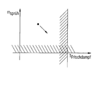
- the fresh water rate sprayed into a temperature control unit for live steam can be set to a value of at least zero.
- a further boundary condition can limit the temperature of the live steam (T live steam ) to a maximum value T max (T live steam ⁇ T max ).
- T live steam the live steam
- T max the maximum value of water spray reduces the live steam temperature. This functional dependence is contained in the balance equations c (x).
- certain optimization variables may also be limited by lower limits x L and upper limits x U.
- this optimization problem is solved with a suitable optimization algorithm.
- the values obtained for the optimization variables are optimized in such a way that the sum of their quadratic distances from the predefined setpoints assumes a minimum value. If a setpoint for an optimization variable x i, which is inappropriate for the system, has been specified, then this discrepant setpoint can be recognized immediately on the solution, since the for this variable, as a result of the optimization calculation resulting value has a considerable compared with the results of the other variables distance from its associated setpoint. For such a case, the setpoint for the corresponding variable is then corrected and the entire optimization calculation is repeated.
- p and u are auxiliary variables.
- the objective function ⁇ i ( p i + u i ) is hereby linear.
Landscapes
- Engineering & Computer Science (AREA)
- Chemical & Material Sciences (AREA)
- Combustion & Propulsion (AREA)
- Mechanical Engineering (AREA)
- General Engineering & Computer Science (AREA)
- Feedback Control In General (AREA)
- Management, Administration, Business Operations System, And Electronic Commerce (AREA)
Abstract
Description
Die Erfindung betrifft ein Verfahren zur Berechnung energie- und verfahrenstechnischer Prozesse, insbesondere des Wärmekreislaufs von Kraftwerken, mittels eines auf mindestens einer Bilanzgleichung des ersten thermodynamischen Hauptsatzes beruhenden rechentechnischen Modells sowie eine Vorrichtung zur Durchführung dieses Verfahrens.The invention relates to a method for calculating energy and process engineering processes, in particular the heat cycle of power plants, by means of a computer based on at least one balance equation of the first law of thermodynamic law computational model and an apparatus for performing this method.
Bei einem im Stand der Technik bekannten gattungsgemäßen Verfahren werden stationäre technische Prozesse im Bereich der Energie- und Verfahrenstechnik durch eine physikalische Modellbildung zu einem mathematischen Modell formuliert. Dieses Modell weist die Bilanzgleichungen des ersten thermodynamischen Hauptsatzes (Massen-, Energie- und Impulsbilanz) auf. Weiterhin können für bestimmte Variablen des Modells feste Werte durch das Einfügen von Randbedingungen in Form von Gleichungen vorgegeben werden. Beispielsweise kann vorgegeben werden, dass kein Kühlwasser in eine Temperiereinheit von frisch erzeugtem Dampf eingesprüht wird. Dazu wird die Bedingung ![]()
![]()
Nach dem Aufstellen der Bilanzgleichungen sowie der die Randbedingungen definierenden Gleichungen im Rahmen einer Phase 1 wird dann durch ein Simulationsprogramm im Rahmen einer Phase 2 eine Newton-Iteration zum Auffinden einer ersten Näherungslösung des vorliegenden Gleichungssystems durchgeführt. Daraufhin wendet sich das Simulationsprogramm wieder Phase 1 zu, in der die Randbedingungsgleichungen anhand der aufgefundenen Näherungslösung überprüft und ggf. abgeändert werden.After establishing the balance equations and the equations defining the boundary conditions in the context of a phase 1, a Newton iteration for finding a first approximation solution of the present equation system is then carried out by a simulation program in the context of a phase 2. thereupon Once again, the simulation program turns to Phase 1, in which the boundary condition equations are checked using the found approximate solution and modified if necessary.
Anknüpfend an das vorstehend angeführte Beispiel wird dabei etwa überprüft, ob die ermittelte Temperatur des Frischdampfes einen bestimmten Grenzwert überschritten hat, in welchem Fall dann eine Randbedingung in Form einer Gleichung eingeführt wird, in der die Frischdampftemperatur auf diesen Grenzwert festgelegt ist. Im Gegenzug wird dann die Zuführrate des Kühlwassers in die Temperiereinheit nicht mehr fest vorgegeben, sondern als Variable definiert. Das heißt die Randbedingung mSprüh = 0 wird aus dem Gleichungssystem herausgenommen, was zur Folge hat, dass die nächste Näherungslösung einen berechneten Wert für mSprüh enthält. Daraufhin tritt der Simulationsalgorithmus wieder in Phase 2 ein, in welcher eine weitere Newton-Iteration vorgenommen wird. Phase 1 und Phase 2 werden solange iterativ wiederholt, bis die Variablen sich innerhalb der gewünschten Bandbreiten befinden und die gewünschten Toleranzen der Näherungsrechnung erfüllt sind.Following on from the example given above, it is checked, for example, whether the determined temperature of the live steam has exceeded a certain limit value, in which case a boundary condition is introduced in the form of an equation in which the live steam temperature is set to this limit value. In return, the feed rate of the cooling water in the temperature control unit is then no longer fixed, but defined as a variable. That is, the boundary condition m spray = 0 is taken out of the equation system, with the result that the next approximate solution contains a calculated value for m spray . The simulation algorithm then returns to Phase 2, where another Newton iteration is performed. Phase 1 and Phase 2 are repeated iteratively until the variables are within the desired bandwidths and the desired tolerances of the approximate calculation are fulfilled.
Die Durchführung dieses Algorithmuses ist relativ umständlich und damit zeitaufwändig. Die so erlangte Lösung muss weiterhin auf Plausibilität geprüft werden. Dabei wird die Lösung auf logische Fehler hin überprüft. Dies umfasst beispielsweise die Prüfung, ob die Temperatur am Ausgang eines Wärmetauschers höher ist als an ihrem Eingang. Weitere logische Überprüfungen beinhalten etwa das Auftreten negativer Lösungen für Variablen, für die derartigen Lösungen ausgeschlossen sind. Werden in dieser Phase Inplausibilitäten entdeckt, muss das gesamte Simulationsmodell überarbeitet und daraufhin neu berechnet werden. Die Fehleridentifizierung wird manuell vorgenommen und erfordert meist aufwändige Untersuchungen.The implementation of this algorithm is relatively cumbersome and therefore time consuming. The solution thus obtained must continue to be checked for plausibility. The solution is checked for logical errors. This includes, for example, checking whether the temperature at the outlet of a heat exchanger is higher than at its inlet. Other logical checks include the occurrence of negative solutions to variables for which such solutions are excluded. If implausibilities are discovered in this phase, the entire simulation model must be revised and then recalculated. The fault identification is done manually and usually requires extensive investigations.
Der Erfindung liegt die Aufgabe zugrunde, die oben genannten Nachteile zu überwinden und insbesondere ein Verfahren sowie eine Vorrichtung zur Berechnung energie- und verfahrenstechnischer Prozesse bereitzustellen, mit dem eine schnellere Berechnung sowie eine schnellere und einfachere Fehlerbehebung möglich ist.The invention has for its object to overcome the above-mentioned disadvantages and in particular a method and to provide a device for the calculation of energy and process engineering processes, allowing faster calculation and faster and easier troubleshooting.
Diese Aufgabe ist erfindungsgemäß mit einem eingangs genannten Verfahren zur Berechnung energie- und verfahrenstechnischer Prozesse gelöst, welches dadurch gekennzeichnet ist, dass die Berechnung in Form einer Optimierungsrechnung ausgeführt wird, in die mindestens eine in Form einer Ungleichung formulierte technische Randbedingung als Nebenbedingung eingeht. Bei einer derartigen Optimierungsrechnung bestimmt ein Optimierungsalgorithmus das Minimum oder Maximum einer Zielfunktion in einem bestimmten, durch Nebenbedingungen in Form von Gleichungen oder Ungleichungen beschriebenen zulässigen Bereich. Zur Optimierung stehen z.B. Verfahren der nicht linearen Programmierung (NLP) zur Verfügung. Indem die mindestens eine technische Randbedingung als Nebenbedingung in die Optimierungsrechnung eingeht, können obere und untere Schranken für die Optimierungsvariablen in der Optimierungsrechnung berücksichtigt werden. Anknüpfend an das vorherige Beispiel kann z.B. die Temperatur des zugeführten Frischdampfes auf eine Maximaltemperatur durch Berücksichtigung der Ungleichung 
Das erfindungsgemäß gelöste Optimierungsproblem lässt sich mathematisch allgemein wie folgt darstellen: ![]()
![]()
![]()
![]()
wobei
Φ die zu minimierende oder maximierende Zielfunktion ist,
x ein Vektor aus kontinuierlichen Optimierungsvariablen mit n durch die Optimierungsrechung zu bestimmenden Elementen ist,
c ein Vektor aus in Form von Gleichungen dargestellten Randbedingungsfunktionen mit m Elementen ist, wobei diese Randbedingungsfunktionen im Wesentlichen aus den Bilanzgleichungen des ersten thermodynamischen Hauptsatzes gebildet sind,
h ein Vektor aus in Form von Ungleichungen dargestellten Randbedingungsfunktionen ist,
x L ein Vektor aus festen unteren Grenzen für die Optimierungsvariablen ist, wobei manche untere Grenzen - ∞ betragen können, in welchem Fall Variablen ohne einer unteren Grenze dargestellt werden, sowie
x u ein Vektor aus festen oberen Grenzen der Optimierungsvariablen ist. Manche oberen Grenzen können + ∞ betragen, in welchem Fall Variablen ohne einer oberen Grenze dargestellt werden.The optimization problem solved according to the invention can be represented mathematically in general as follows: ![]()
![]()
![]()
![]()
in which
Φ is the objective function to be minimized or maximized,
x is a vector of continuous optimization variables with n elements to be determined by the optimization calculation,
c is a vector of boundary condition functions with m elements represented in the form of equations, these boundary condition functions essentially being formed from the balance equations of the first thermodynamic law,
h is a vector of constraint functions represented in the form of inequalities,
x L is a vector of fixed lower bounds for the optimization variables, some of which may be lower bounds - ∞, in which case variables without a lower bound are represented, as well
x u is a vector of fixed upper bounds of the optimization variable. Some upper bounds can be + ∞, in which case variables without an upper bound are represented.
Es wird angemerkt, dass sowohl der Ausdruck (5) als auch der Ausdruck (6) Randbedingungen in Form von Ungleichungen darstellen und die Darstellung mit oberen und unteren Grenzen gemäß Ausdruck (6) lediglich eine vereinfachte Darstellung von entsprechend formulierten Ungleichungen gemäß Ausdruck(5) ist.It is noted that both the expression (5) and the expression (6) represent boundary conditions in the form of inequalities and the representation with upper and lower limits according to expression (6) merely a simplified representation of correspondingly formulated inequalities according to expression (5). is.
Die Erfindung beruht auf der Erkenntnis, dass mittels der erfindungsgemäß in Form einer Optimierungsrechnung ausgeführten Berechnung des physikalischen Modells eine inhärente Berechnung aller technischer Randbedingungen möglich ist. Damit ist eine Berechnung des entsprechenden energie- bzw. verfahrenstechnischen Prozesses in einem durchgängigen Berechnungszyklus möglich. Iterative Durchläufe verschiedener Berechnungsphasen mit dazwischen vorgenommenen Anpassungen der Randbedingungen, wie bei der auf dem Simulationsmodell beruhenden Berechnung aus dem Stand der Technik sind nicht mehr erforderlich. Da weiterhin eine Gesamtoptimierung des Systems vorgenommen wird, ist eine Behebung möglicher Fehler bei in der Form von Sollwerten vorgegeben Randbedingungen für bestimmte Variablen schneller möglich. Ein möglicherweise unpassender Sollwert für eine Variable ist nämlich aus dem Optimierungsergebnis leicht ersichtlich, da der vom Optimierungsalgorithmus berechnete Variablenwert sich in der Regel erheblich vom unpassenden Sollwert unterscheidet. Da der Optimierungsalgorithmus bestrebt ist, eine Gesamtheit vieler Variablen zu optimieren, wird im Optimierungsergebnis die entsprechende einzelne Variable nicht sehr nahe an dem unpassenden Sollwert liegen, da dadurch in der Regel das Ergebnis für viele andere Variablen wesentlich ungünstiger ausfällt, wodurch das Optimierungsergebnis als Ganzes übermäßig verschlechtert würde.The invention is based on the recognition that by means of the calculation of the physical model carried out according to the invention in the form of an optimization calculation, an inherent calculation of all technical boundary conditions is possible. Thus, a calculation of the corresponding energy or process engineering process in a continuous calculation cycle is possible. Iterative runs of different calculation phases with adjustments of the boundary conditions between them, as in the simulation model based calculation of the prior art are no longer necessary. Since an overall optimization of the system continues to be carried out, it is possible to remedy possible errors in the case of specified boundary conditions for certain variables more quickly. A possibly inappropriate setpoint for a variable is in fact easily apparent from the optimization result, since the variable value calculated by the optimization algorithm generally differs significantly from the inappropriate setpoint. Since the optimization algorithm strives to optimize a set of many variables, in the optimization result, the corresponding single variable will not be very close to the inappropriate setpoint, as this will generally result in much less favorable results for many other variables, thereby rendering the optimization result as a whole excessive would be worsened.
Bei einer vorteilhaften Weiterbildung der Erfindung geht mindestens eine logische Bedingung als Nebenbedingung in die Optimierungsrechnung ein. Vorteilhafterweise geht diese mindestens eine logische Bedingung in Form einer Ungleichung in die Optimierungsrechnung ein. Eine solche logische Bedingung kann z.B. Temperaturen an zwei verschiedenen Stellen einer Vorrichtung in Form einer Ungleichung zueinander in Beziehung setzen. So kann zum Beispiel vorgegeben sein, dass die Temperatur an einem Wärmetauschereingang höher sein muss als die Temperatur am Wärmetauscherausgang. Da derartige logische Bedingungen in der erfindungsgemäßen Ausführungsform direkt von dem Berechnungsverfahren berücksichtigt werden, ist eine nachträgliche Plausibilitätsprüfung diesbezüglich nicht mehr nötig.In an advantageous development of the invention, at least one logical condition enters into the optimization calculation as a secondary condition. Advantageously, this at least one logical condition enters into the optimization calculation in the form of an inequality. Such a logical condition may e.g. Relate temperatures at two different locations of a device in the form of an inequality. For example, it may be specified that the temperature at a heat exchanger inlet must be higher than the temperature at the heat exchanger outlet. Since such logical conditions are taken into account directly by the calculation method in the embodiment according to the invention, a subsequent plausibility check in this regard is no longer necessary.
Vorteilhafterweise wird bei dem erfindungsgemäßen Berechnungsverfahren eine durch das rechentechnische Modell gegebene quadratische Simulationsaufgabe in eine Optimierungsaufgabe umformuliert. Dabei werden etwa die in Form von Gleichungen im rechentechnischen Modell vorliegenden Randbedingungen in die Zielfunktion der Optimierungsrechnung übertragen. Die verbleibenden Bilanzgleichungen aus dem rechentechnischen Modell werden bei der Optimierungsrechnung nun als Nebenbedingungen berücksichtigt.Advantageously, in the inventive calculation method, a quadratic simulation task given by the computational model is reformulated into an optimization task. In this case, for example, the existing in the form of equations in the computational model boundary conditions transferred to the objective function of the optimization calculation. The remaining balance equations from the computational model are now considered as constraints in the optimization calculation.
Darüber hinaus liegt der Optimierungsrechnung vorteilhafterweise eine quadratische Zielfunktion zur Berechnung der kleinsten quadratischen Abstände der Optimierungsvariablen von vorgebenden Sollwerten zugrunde. Die in der Optimierungsaufgabe zu minimierende Zielfunktion besteht dann aus der Summe der quadratischen Abstände der Optimierungsvariablen oder davon abhängigen Umwandlungsfunktionen von den jeweils zugeordneten Sollwerten. Mit einer derartigen Zielfunktion ist ein schnelles Auffinden von unpassend gewählten Sollwerten und damit eine schnelle Fehlerbehebung möglich. Dies liegt darin begründet, dass in der von der Optimierungsrechnung aufgefundenen Lösung die Gesamtheit der Optimierungsvariablen möglichst nahe an den jeweils zugeordneten Sollwerten liegt. Ist ein bestimmter Sollwert jedoch unpassend gewählt, so nähert der Optimierungsalgorithmus die diesem zugeordnete Variable nicht nennenswert an diesen Sollwert an, wenn dadurch der Abstand der anderen Optimierungsvariablen zu deren Sollwerten in Summe stärker steigen würde, was bei einem aus technischer Sicht unstimmigen einzelnen Sollwert der Fall wäre. Damit ist in der Regel aufgrund eines großen Abstandes einer Optimierungsvariablen zu deren Sollwert ein solcher unpassender Sollwert in der aus der Optimierungsrechnung hervorgehenden Lösung sofort ersichtlich und kann damit gezielt korrigiert werden.In addition, the optimization calculation is advantageously based on a quadratic target function for calculating the smallest quadratic distances of the optimization variables of predefinable target values. The objective function to be minimized in the optimization task then consists of the sum of the quadratic distances of the optimization variables or conversion functions dependent thereon from the respectively assigned nominal values. With such an objective function, it is possible to quickly find inappropriately selected setpoint values and thus fast troubleshooting. This is due to the fact that in the solution found by the optimization calculation, the totality of the optimization variables is as close as possible to the respective assigned setpoint values. However, if a certain setpoint is chosen inappropriately, the optimization algorithm does not appreciably approximate the variable associated therewith to this setpoint, if this would result in a greater increase in the distance of the other optimization variables to their setpoints, which would be the case for a single setpoint that is technically inconsistent would. As a result, due to a large distance between an optimization variable and its desired value, such an inappropriate target value is usually immediately apparent in the solution resulting from the optimization calculation and can thus be corrected in a targeted manner.
Manche Optimierungsalgorithmen arbeiten jedoch effizienter mit linearen Zielfunktionen als mit quadratischen Zielfunktionen, insbesondere erzeugen quadratische Zielfunktionen bei manchen Algorithmen eine beträchtliche Anzahl an Einträgen in die Hesse-Matrix, wodurch zu viele Freiheitsgrade für die Aktualisierung der Hesse-Matrix entstehen können. Zur Verwendung derartiger Algorithmen ist es daher zweckmäßig, wenn der Optimierungsrechnung eine lineare Zielfunktion zugrunde liegt.However, some optimization algorithms work more efficiently with linear objective functions than with quadratic objective functions; in particular, quadratic objective functions in some algorithms generate a considerable number of entries in the Hesse matrix, which can lead to too many degrees of freedom for updating the Hesse matrix. To use such algorithms, it is therefore appropriate if the Optimization calculation is based on a linear objective function.
Weiterhin ist es vorteilhaft, wenn auch mindestens eine als Gleichung formulierte technische Randbedingung als Nebenbedingung in die Optimierungsrechnung eingeht. Dies erhöht die Flexibilität bei der Definierung des Optimierungsproblems.Furthermore, it is advantageous if at least one technical boundary condition formulated as an equation enters into the optimization calculation as a secondary condition. This increases the flexibility in defining the optimization problem.
Weiterhin ist es zweckmäßig, wenn mindestens eine logische Bedingung aus dem zweiten thermodynamischen Hauptsatz abgeleitet ist. Das heißt, bestimmte aus dem Entropiesatz resultierende Ungleichungen zwischen Temperaturen an unterschiedlichen Orten eines Systems können schon als Nebenbedingung in die Optimierungsrechnung einfließen. Eine nachträgliche Plausibilitätsprüfung der vom Berechnungsalgorithmus aufgefundenen Lösung in Bezug auf etwa zwingend notwendige Entropiezunahmen bei irreversiblen Prozessen wird damit überflüssig.Furthermore, it is expedient if at least one logical condition is derived from the second thermodynamic law. That is, certain inequalities between temperatures at different locations of a system resulting from the entropy set can already be included in the optimization calculation as a secondary condition. A subsequent plausibility check of the solution found by the calculation algorithm with respect to approximately mandatory entropy increases in irreversible processes is thus superfluous.
Die Erfindung betrifft ferner eine Vorrichtung zur Durchführung des erfindungsgemäßen Verfahrens.The invention further relates to a device for carrying out the method according to the invention.
Nachfolgend wird ein Ausführungsbeispiel der Erfindung anhand der beigefügten schematischen Zeichnung näher erläutert. In dieser zeigt die Fig. eine Veranschaulichung des Lösungsraums zweier durch technische Randbedingungen in Form von Ungleichungen beschränkten Optimierungsvariablen.An embodiment of the invention will be explained in more detail with reference to the accompanying schematic drawing. In the figure, the figure shows an illustration of the solution space of two optimization variables bounded by technical boundary conditions in the form of inequalities.
Das nachstehend beschriebene Ausführungsbeispiel der Erfindung dient der Berechnung des Wärmekreislaufs eines Heizkraftwerks. Dazu wird zunächst der Wärmekreislauf mittels Bilanzgleichungen c(x) des thermodynamischen Hauptsatzes (Massen-, Energie- und Impulsbilanz) als Funktion von Optimierungsvariablen xi beschrieben. Daraufhin werden Sollwerte ys,i dieser Optimierungsvariablen xi bzw. von aus den Optimierungsvariablen xi unter Verwendung eines internen Umwandlungsvektors b(xi) hervorgehenden Variablen definiert. Ein solcher interner Umwandlungsvektor b(xi) kann z.B. die Beziehung zwischen der als Sollwert vorgegebenen Entropie und der als Optimierungsvariable vorgebenden Temperatur darstellen. Weiterhin werden Randbedingungen h(x) in Form von Ungleichungen für die Optimierungsvariablen xi definiert.The embodiment of the invention described below is used to calculate the heat cycle of a cogeneration plant. For this purpose, the heat cycle is first described by means of balance equations c (x) of the thermodynamic law (mass, energy and momentum balance) as a function of optimization variables x i . Then, command values are y s, i this optimization variables x i and of the optimization of variable i of an internal transformation vector b (x i) arising variable x defined using. Such an internal conversion vector b (x i ) can, for example, the relationship represent between the entropy specified as the desired value and the temperature that predetermines as the optimization variable. Furthermore, boundary conditions h (x) are defined in the form of inequalities for the optimization variables x i .
Bezug nehmend auf die Fig. kann in einer solchen Randbedingung z.B. mittels der Ungleichung mSprüh ≥ 0 die in eine Temperiereinheit für Frischdampf eingesprühte Frischwasserrate auf einen Wert von mindestens 0 festgelegt werden. Eine weitere Randbedingung kann die Temperatur des Frischdampfes (TFrischdampf) auf einen Maximalwert Tmax begrenzen (TFrischdampf ≤ Tmax) Die beiden Optimierungsvariablen mSprüh und TFrischdampf sind jedoch funktional voneinander abhängig, da eine höhere Zugabe von Sprühwasser die Frischdampftemperatur verringert. Diese funktionale Abhängigkeit ist in den Bilanzgleichungen c(x) enthalten. Weiterhin können bestimmte Optimierungsvariablen auch durch untere Grenzen xL und obere Grenzen xU beschränkt sein.With reference to the figures , in such a boundary condition, for example by means of the inequality m spray ≥ 0, the fresh water rate sprayed into a temperature control unit for live steam can be set to a value of at least zero. A further boundary condition can limit the temperature of the live steam (T live steam ) to a maximum value T max (T live steam ≦ T max ). However, the two optimization variables m spray and T live steam are functionally interdependent since a higher addition of water spray reduces the live steam temperature. This functional dependence is contained in the balance equations c (x). Furthermore, certain optimization variables may also be limited by lower limits x L and upper limits x U.
Daraufhin wird das folgende Optimierungsproblem zur Berechnung der kleinsten quadratischen Abstände der Optimierungsvariablen von den vorgegebenen Sollwerten aufgestellt: 
![]()
![]()
![]()
![]()
![]()
![]()
Daraufhin wird dieses Optimierungsproblem mit einem geeigneten Optimierungsalgorithmus gelöst. Die als Ergebnis erhaltenen Werte für die Optimierungsvariablen sind dahingehend optimiert, dass die Summe ihrer quadratischen Abstände von den vorgegebenen Sollwerten einen Minimalwert einnimmt. Sollte ein für das System unpassender Sollwert für eine Optimierungsvariable xi vorgegeben worden sein, so lässt sich dieser unstimmige Sollwert sofort auf der Lösung erkennen, da der für diese Variable als Ergebnis aus der Optimierungsrechnung hervorgehende Wert einen im Vergleich mit den Ergebnissen der anderen Variablen erheblichen Abstand von dem ihm zugeordneten Sollwert aufweist. Für einen solchen Fall wird dann der Sollwert für die entsprechende Variable berichtigt und die gesamte Optimierungsrechnung wiederholt.Then this optimization problem is solved with a suitable optimization algorithm. The values obtained for the optimization variables are optimized in such a way that the sum of their quadratic distances from the predefined setpoints assumes a minimum value. If a setpoint for an optimization variable x i, which is inappropriate for the system, has been specified, then this discrepant setpoint can be recognized immediately on the solution, since the for this variable, as a result of the optimization calculation resulting value has a considerable compared with the results of the other variables distance from its associated setpoint. For such a case, the setpoint for the corresponding variable is then corrected and the entire optimization calculation is repeated.
Als Alternative zum oben dargestellten Lösungsansatz der kleinsten Quadrate kann auch ein linearer Lösungsansatz wie folgt gewählt werden: 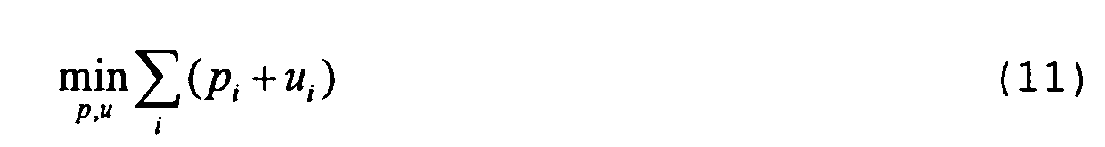
![]()
![]()
![]()
![]()
![]()
![]()
![]()
![]()
![]()
![]()
Hierbei sind p und u Hilfsvariablen. Die Zielfunktion ![]()
![]()
Claims (8)
dadurch gekennzeichnet, dass die Berechnung in Form einer Optimierungsrechnung ausgeführt wird, in die mindestens eine in Form einer Ungleichung formulierte technische Randbedingung als Nebenbedingung eingeht.Method for calculating energy and process engineering processes, in particular the heat cycle of power plants, by means of a computational model based on at least one balance equation of the first thermodynamic law,
characterized in that the calculation is performed in the form of an optimization calculation, in which at least one formulated in the form of an inequality technical boundary condition enters as a secondary condition.
dadurch gekennzeichnet, dass mindestens eine logische Bedingung als Nebenbedingung in die Optimierungsrechnung eingeht.Method according to claim 1,
characterized in that at least one logical condition enters as a constraint in the optimization calculation.
gekennzeichnet durch eine Umformulierung einer durch das rechentechnische Modell gegebenen quadratischen Simulationsaufgabe in eine Optimierungsaufgabe.Method according to claim 1 or 2,
characterized by reformulating a quadratic simulation task given by the computational model into an optimization task.
dadurch gekennzeichnet, dass der Optimierungsrechnung eine quadratische Zielfunktion zur Berechnung der kleinsten quadratischen Abstände der Optimierungsvariablen (xi) von vorgegebenen Sollwerten zugrunde liegt.Method according to one of the preceding claims,
characterized in that the optimization calculation is based on a quadratic target function for the calculation of the smallest quadratic distances of the optimization variables (x i ) from predetermined target values.
dadurch gekennzeichnet, dass der Optimierungsrechnung eine lineare Zielfunktion zugrunde liegt.Method according to one of the preceding claims,
characterized in that the optimization calculation is based on a linear objective function.
dadurch gekennzeichnet, dass mindestens eine logische Bedingung aus dem zweiten thermodynamischen Hauptsatz abgeleitet ist.Method according to one of the preceding claims,
characterized in that at least one logical condition is derived from the second thermodynamic law.
Priority Applications (4)
| Application Number | Priority Date | Filing Date | Title |
|---|---|---|---|
| EP05003691A EP1701005A1 (en) | 2005-02-21 | 2005-02-21 | Method and apparatus for the calculation of energy and technical processes |
| EP06708366A EP1851417A2 (en) | 2005-02-21 | 2006-02-17 | Method and device for calculating energy and technical processes |
| CN2006800055949A CN101124386B (en) | 2005-02-21 | 2006-02-17 | Method and device for calculating energy and technical processes |
| PCT/EP2006/060078 WO2006087382A2 (en) | 2005-02-21 | 2006-02-17 | Method and device for calculating energy and technical processes |
Applications Claiming Priority (1)
| Application Number | Priority Date | Filing Date | Title |
|---|---|---|---|
| EP05003691A EP1701005A1 (en) | 2005-02-21 | 2005-02-21 | Method and apparatus for the calculation of energy and technical processes |
Publications (1)
| Publication Number | Publication Date |
|---|---|
| EP1701005A1 true EP1701005A1 (en) | 2006-09-13 |
Family
ID=34933859
Family Applications (2)
| Application Number | Title | Priority Date | Filing Date |
|---|---|---|---|
| EP05003691A Withdrawn EP1701005A1 (en) | 2005-02-21 | 2005-02-21 | Method and apparatus for the calculation of energy and technical processes |
| EP06708366A Withdrawn EP1851417A2 (en) | 2005-02-21 | 2006-02-17 | Method and device for calculating energy and technical processes |
Family Applications After (1)
| Application Number | Title | Priority Date | Filing Date |
|---|---|---|---|
| EP06708366A Withdrawn EP1851417A2 (en) | 2005-02-21 | 2006-02-17 | Method and device for calculating energy and technical processes |
Country Status (3)
| Country | Link |
|---|---|
| EP (2) | EP1701005A1 (en) |
| CN (1) | CN101124386B (en) |
| WO (1) | WO2006087382A2 (en) |
Families Citing this family (1)
| Publication number | Priority date | Publication date | Assignee | Title |
|---|---|---|---|---|
| CN110717273B (en) * | 2019-10-11 | 2023-03-17 | 内蒙古第一机械集团股份有限公司 | Technological process simulation boundary condition construction method |
Citations (3)
| Publication number | Priority date | Publication date | Assignee | Title |
|---|---|---|---|---|
| US4577270A (en) * | 1980-07-04 | 1986-03-18 | Hitachi, Ltd. | Plant control method |
| EP0731397A1 (en) * | 1994-09-26 | 1996-09-11 | Kabushiki Kaisha Toshiba | Method and system for optimizing plant utility |
| JP2004060462A (en) * | 2002-07-25 | 2004-02-26 | Honda Motor Co Ltd | Rankine cycle device |
-
2005
- 2005-02-21 EP EP05003691A patent/EP1701005A1/en not_active Withdrawn
-
2006
- 2006-02-17 CN CN2006800055949A patent/CN101124386B/en not_active Expired - Fee Related
- 2006-02-17 EP EP06708366A patent/EP1851417A2/en not_active Withdrawn
- 2006-02-17 WO PCT/EP2006/060078 patent/WO2006087382A2/en active Application Filing
Patent Citations (3)
| Publication number | Priority date | Publication date | Assignee | Title |
|---|---|---|---|---|
| US4577270A (en) * | 1980-07-04 | 1986-03-18 | Hitachi, Ltd. | Plant control method |
| EP0731397A1 (en) * | 1994-09-26 | 1996-09-11 | Kabushiki Kaisha Toshiba | Method and system for optimizing plant utility |
| JP2004060462A (en) * | 2002-07-25 | 2004-02-26 | Honda Motor Co Ltd | Rankine cycle device |
Non-Patent Citations (2)
| Title |
|---|
| GICQUEL R: "METHODE D'OPTIMISATION SYSTEMIQUE BASEE SUR L'INTEGRATION THERMIQUEPAR EXTENSION DE LA METHODE DU PINCEMENT APPLICATION A LA COGENERATION AVEC PRODUCTION DE VAPEUR", REVUE GENERALE DE THERMIQUE, ELSEVIER EDITIONS SCIENTIFIQUES ET MEDICALES,PARIS, FR, vol. 34, no. 406, 1 October 1995 (1995-10-01), pages 579S - 607S, XP000543739, ISSN: 0035-3159 * |
| MOSLEHI K: "OPTIMIZATION OF MULTIPLANT COGENERATION SYSTEM OPERATION INCLUDING ELECTRIC AND STEAM NETWORKS", IEEE TRANSACTIONS ON POWER SYSTEMS, IEEE INC. NEW YORK, US, vol. 6, no. 2, 1 May 1991 (1991-05-01), pages 484 - 490, XP000220544, ISSN: 0885-8950 * |
Also Published As
| Publication number | Publication date |
|---|---|
| CN101124386B (en) | 2011-11-16 |
| WO2006087382A2 (en) | 2006-08-24 |
| CN101124386A (en) | 2008-02-13 |
| WO2006087382A3 (en) | 2006-11-16 |
| EP1851417A2 (en) | 2007-11-07 |
Similar Documents
| Publication | Publication Date | Title |
|---|---|---|
| DE602005002839T2 (en) | PROCESSING OF INDUSTRIAL PRODUCTION PROCESSES | |
| DE69315423T2 (en) | Neuro-Pid controller | |
| EP2296062B1 (en) | Method for computer-supported learning of a control and/or regulation of a technical system | |
| DE3786977T2 (en) | Process control systems and processes. | |
| EP2999998B1 (en) | Methods for ascertaining a model of an output variable of a technical system | |
| EP2880499B1 (en) | Method for controlling and/or regulating a technical system in a computer-assisted manner | |
| EP3511126A1 (en) | Method for computer-assisted planning of a process which can be executed by a robot | |
| EP2411735B1 (en) | Method and device for regulating the temperature of steam for a steam power plant | |
| EP2943841B1 (en) | Method for the computerized control and/or regulation of a technical system | |
| DE102018129810A1 (en) | Method and device for controlling a number of energy-feeding and / or energy-consuming units | |
| EP1701005A1 (en) | Method and apparatus for the calculation of energy and technical processes | |
| EP3542229B1 (en) | Device and method for determining the parameters of a control device | |
| EP3323025B1 (en) | Method and device for operating a technical system | |
| DE202019100641U1 (en) | Training device for AI modules | |
| DE102020201215A1 (en) | Method for operating an industrial plant | |
| EP2394031B1 (en) | Method for installation control in a power plant | |
| DE102019107040A1 (en) | Method of setting up a controller | |
| DE10011607A1 (en) | Operating method for technical system enabling intelligent operating parameter setting for technical system with several system parts for optimal system operation | |
| EP1483633B1 (en) | Method for simulating a technical system and simulator | |
| DE102019210734A1 (en) | Operating method of an electric heater | |
| DE102009009328B4 (en) | Method for reducing structural vibrations and control device for this purpose | |
| DE102021212157A1 (en) | Process for improving the statistical description of measured values | |
| DE102005010027B4 (en) | Method for the computer-aided operation of a technical system | |
| EP3916638A1 (en) | Computer based design method and design system | |
| WO2020151927A1 (en) | Computer-aided method for simulating the operation of an energy system, and energy management system |
Legal Events
| Date | Code | Title | Description |
|---|---|---|---|
| PUAI | Public reference made under article 153(3) epc to a published international application that has entered the european phase |
Free format text: ORIGINAL CODE: 0009012 |
|
| AK | Designated contracting states |
Kind code of ref document: A1 Designated state(s): AT BE BG CH CY CZ DE DK EE ES FI FR GB GR HU IE IS IT LI LT LU MC NL PL PT RO SE SI SK TR |
|
| AX | Request for extension of the european patent |
Extension state: AL BA HR LV MK YU |
|
| AKX | Designation fees paid | ||
| STAA | Information on the status of an ep patent application or granted ep patent |
Free format text: STATUS: THE APPLICATION IS DEEMED TO BE WITHDRAWN |
|
| 18D | Application deemed to be withdrawn |
Effective date: 20070314 |
|
| REG | Reference to a national code |
Ref country code: DE Ref legal event code: 8566 |