EP1600351A1 - Method and system for detecting defects and hazardous conditions in passing rail vehicles - Google Patents
Method and system for detecting defects and hazardous conditions in passing rail vehicles Download PDFInfo
- Publication number
- EP1600351A1 EP1600351A1 EP04076047A EP04076047A EP1600351A1 EP 1600351 A1 EP1600351 A1 EP 1600351A1 EP 04076047 A EP04076047 A EP 04076047A EP 04076047 A EP04076047 A EP 04076047A EP 1600351 A1 EP1600351 A1 EP 1600351A1
- Authority
- EP
- European Patent Office
- Prior art keywords
- vehicle
- data
- sensors
- vehicles
- rail vehicle
- Prior art date
- Legal status (The legal status is an assumption and is not a legal conclusion. Google has not performed a legal analysis and makes no representation as to the accuracy of the status listed.)
- Granted
Links
- 238000000034 method Methods 0.000 title claims abstract description 467
- 231100001261 hazardous Toxicity 0.000 title claims abstract description 118
- 230000007547 defect Effects 0.000 title claims abstract description 117
- 238000001514 detection method Methods 0.000 claims abstract description 186
- 238000010276 construction Methods 0.000 claims abstract description 66
- 230000011664 signaling Effects 0.000 claims abstract description 46
- 238000013021 overheating Methods 0.000 claims abstract description 45
- 238000007620 mathematical function Methods 0.000 claims abstract description 15
- 239000000470 constituent Substances 0.000 claims abstract description 10
- 238000005259 measurement Methods 0.000 claims description 576
- 230000006870 function Effects 0.000 claims description 249
- 238000012545 processing Methods 0.000 claims description 128
- 238000009434 installation Methods 0.000 claims description 125
- 238000003384 imaging method Methods 0.000 claims description 82
- 238000011068 loading method Methods 0.000 claims description 69
- 230000009466 transformation Effects 0.000 claims description 61
- 230000005855 radiation Effects 0.000 claims description 59
- 238000005096 rolling process Methods 0.000 claims description 59
- 230000003287 optical effect Effects 0.000 claims description 48
- 238000004422 calculation algorithm Methods 0.000 claims description 46
- 238000012423 maintenance Methods 0.000 claims description 42
- 238000012015 optical character recognition Methods 0.000 claims description 38
- 230000032258 transport Effects 0.000 claims description 37
- 230000014509 gene expression Effects 0.000 claims description 36
- 238000004891 communication Methods 0.000 claims description 35
- 230000002159 abnormal effect Effects 0.000 claims description 33
- 238000003491 array Methods 0.000 claims description 33
- 239000013598 vector Substances 0.000 claims description 33
- 238000005286 illumination Methods 0.000 claims description 30
- 230000000670 limiting effect Effects 0.000 claims description 26
- 239000000872 buffer Substances 0.000 claims description 25
- 230000033001 locomotion Effects 0.000 claims description 22
- 238000010438 heat treatment Methods 0.000 claims description 20
- 230000001133 acceleration Effects 0.000 claims description 18
- 230000009471 action Effects 0.000 claims description 12
- 230000033228 biological regulation Effects 0.000 claims description 6
- 230000000007 visual effect Effects 0.000 claims description 6
- WPYVAWXEWQSOGY-UHFFFAOYSA-N indium antimonide Chemical compound [Sb]#[In] WPYVAWXEWQSOGY-UHFFFAOYSA-N 0.000 claims description 3
- MARUHZGHZWCEQU-UHFFFAOYSA-N 5-phenyl-2h-tetrazole Chemical compound C1=CC=CC=C1C1=NNN=N1 MARUHZGHZWCEQU-UHFFFAOYSA-N 0.000 claims 2
- 230000008520 organization Effects 0.000 claims 2
- GGYFMLJDMAMTAB-UHFFFAOYSA-N selanylidenelead Chemical compound [Pb]=[Se] GGYFMLJDMAMTAB-UHFFFAOYSA-N 0.000 claims 2
- 230000008569 process Effects 0.000 description 143
- 230000008901 benefit Effects 0.000 description 58
- 238000006073 displacement reaction Methods 0.000 description 42
- 230000035945 sensitivity Effects 0.000 description 32
- 101000834981 Homo sapiens Testis, prostate and placenta-expressed protein Proteins 0.000 description 31
- IDCBOTIENDVCBQ-UHFFFAOYSA-N TEPP Chemical compound CCOP(=O)(OCC)OP(=O)(OCC)OCC IDCBOTIENDVCBQ-UHFFFAOYSA-N 0.000 description 31
- 102100026164 Testis, prostate and placenta-expressed protein Human genes 0.000 description 31
- 238000013461 design Methods 0.000 description 31
- 230000010354 integration Effects 0.000 description 29
- 230000009467 reduction Effects 0.000 description 28
- 239000011295 pitch Substances 0.000 description 27
- 239000000047 product Substances 0.000 description 25
- 230000018109 developmental process Effects 0.000 description 24
- 230000000694 effects Effects 0.000 description 23
- 238000011161 development Methods 0.000 description 21
- 101001124620 Curvularia inaequalis Vanadium chloroperoxidase Proteins 0.000 description 20
- 230000008859 change Effects 0.000 description 20
- 238000003745 diagnosis Methods 0.000 description 20
- 230000003137 locomotive effect Effects 0.000 description 20
- 238000012937 correction Methods 0.000 description 18
- 230000010355 oscillation Effects 0.000 description 18
- 238000002405 diagnostic procedure Methods 0.000 description 17
- 238000003672 processing method Methods 0.000 description 16
- 230000004044 response Effects 0.000 description 16
- 238000005070 sampling Methods 0.000 description 15
- 230000006872 improvement Effects 0.000 description 14
- 238000007726 management method Methods 0.000 description 14
- 238000012795 verification Methods 0.000 description 14
- 239000007787 solid Substances 0.000 description 12
- 230000008093 supporting effect Effects 0.000 description 12
- 101100459998 Saccharomyces cerevisiae (strain ATCC 204508 / S288c) NDJ1 gene Proteins 0.000 description 11
- 101100205955 Schizosaccharomyces pombe (strain 972 / ATCC 24843) tam1 gene Proteins 0.000 description 11
- 101150028282 TMT-1 gene Proteins 0.000 description 11
- 230000004888 barrier function Effects 0.000 description 11
- 206010012411 Derailment Diseases 0.000 description 10
- 238000005266 casting Methods 0.000 description 10
- 238000005516 engineering process Methods 0.000 description 10
- 238000007781 pre-processing Methods 0.000 description 10
- 238000009529 body temperature measurement Methods 0.000 description 9
- 238000013213 extrapolation Methods 0.000 description 9
- 238000012544 monitoring process Methods 0.000 description 9
- 230000002829 reductive effect Effects 0.000 description 9
- 238000013519 translation Methods 0.000 description 9
- 238000004364 calculation method Methods 0.000 description 8
- 238000009826 distribution Methods 0.000 description 8
- 239000000428 dust Substances 0.000 description 8
- 230000036962 time dependent Effects 0.000 description 8
- 238000012546 transfer Methods 0.000 description 8
- YBNMDCCMCLUHBL-UHFFFAOYSA-N (2,5-dioxopyrrolidin-1-yl) 4-pyren-1-ylbutanoate Chemical compound C=1C=C(C2=C34)C=CC3=CC=CC4=CC=C2C=1CCCC(=O)ON1C(=O)CCC1=O YBNMDCCMCLUHBL-UHFFFAOYSA-N 0.000 description 7
- 238000012935 Averaging Methods 0.000 description 7
- 239000003570 air Substances 0.000 description 7
- 238000004458 analytical method Methods 0.000 description 7
- 238000011156 evaluation Methods 0.000 description 7
- 230000007717 exclusion Effects 0.000 description 7
- 238000001914 filtration Methods 0.000 description 7
- 230000007704 transition Effects 0.000 description 7
- 230000001960 triggered effect Effects 0.000 description 7
- 238000005303 weighing Methods 0.000 description 7
- 101100006844 Schizosaccharomyces pombe (strain 972 / ATCC 24843) cmc4 gene Proteins 0.000 description 6
- 238000013459 approach Methods 0.000 description 6
- 239000003795 chemical substances by application Substances 0.000 description 6
- 239000002131 composite material Substances 0.000 description 6
- 230000003247 decreasing effect Effects 0.000 description 6
- 210000000887 face Anatomy 0.000 description 6
- 230000001965 increasing effect Effects 0.000 description 6
- 230000006855 networking Effects 0.000 description 6
- 230000001681 protective effect Effects 0.000 description 6
- 239000000779 smoke Substances 0.000 description 6
- 230000026676 system process Effects 0.000 description 6
- 101100060558 Schizosaccharomyces pombe (strain 972 / ATCC 24843) coa3 gene Proteins 0.000 description 5
- 101100424482 Schizosaccharomyces pombe (strain 972 / ATCC 24843) tam5 gene Proteins 0.000 description 5
- XUIMIQQOPSSXEZ-UHFFFAOYSA-N Silicon Chemical compound [Si] XUIMIQQOPSSXEZ-UHFFFAOYSA-N 0.000 description 5
- 230000001143 conditioned effect Effects 0.000 description 5
- 230000006866 deterioration Effects 0.000 description 5
- 239000011159 matrix material Substances 0.000 description 5
- 238000012986 modification Methods 0.000 description 5
- 230000004048 modification Effects 0.000 description 5
- 230000036961 partial effect Effects 0.000 description 5
- 229910052710 silicon Inorganic materials 0.000 description 5
- 239000010703 silicon Substances 0.000 description 5
- 238000012360 testing method Methods 0.000 description 5
- 239000002699 waste material Substances 0.000 description 5
- 238000005452 bending Methods 0.000 description 4
- 230000005540 biological transmission Effects 0.000 description 4
- 230000003139 buffering effect Effects 0.000 description 4
- 238000006243 chemical reaction Methods 0.000 description 4
- 239000003245 coal Substances 0.000 description 4
- 230000001419 dependent effect Effects 0.000 description 4
- 238000007710 freezing Methods 0.000 description 4
- 230000008014 freezing Effects 0.000 description 4
- 239000007789 gas Substances 0.000 description 4
- 230000004807 localization Effects 0.000 description 4
- 238000004519 manufacturing process Methods 0.000 description 4
- 230000007246 mechanism Effects 0.000 description 4
- 239000000203 mixture Substances 0.000 description 4
- 239000002245 particle Substances 0.000 description 4
- 238000002360 preparation method Methods 0.000 description 4
- 238000012552 review Methods 0.000 description 4
- 239000000523 sample Substances 0.000 description 4
- 238000000926 separation method Methods 0.000 description 4
- 230000003595 spectral effect Effects 0.000 description 4
- 238000001228 spectrum Methods 0.000 description 4
- 241000252506 Characiformes Species 0.000 description 3
- 241001669679 Eleotris Species 0.000 description 3
- 208000001836 Firesetting Behavior Diseases 0.000 description 3
- 229910000661 Mercury cadmium telluride Inorganic materials 0.000 description 3
- 230000003044 adaptive effect Effects 0.000 description 3
- 238000004378 air conditioning Methods 0.000 description 3
- 239000003086 colorant Substances 0.000 description 3
- 238000000205 computational method Methods 0.000 description 3
- 238000011960 computer-aided design Methods 0.000 description 3
- 230000006378 damage Effects 0.000 description 3
- 230000005672 electromagnetic field Effects 0.000 description 3
- 230000005670 electromagnetic radiation Effects 0.000 description 3
- 238000000227 grinding Methods 0.000 description 3
- 238000009499 grossing Methods 0.000 description 3
- 230000012010 growth Effects 0.000 description 3
- 239000000383 hazardous chemical Substances 0.000 description 3
- 238000003331 infrared imaging Methods 0.000 description 3
- 238000007689 inspection Methods 0.000 description 3
- 239000000463 material Substances 0.000 description 3
- 238000012216 screening Methods 0.000 description 3
- 230000035939 shock Effects 0.000 description 3
- 239000000126 substance Substances 0.000 description 3
- 230000001052 transient effect Effects 0.000 description 3
- 238000010200 validation analysis Methods 0.000 description 3
- 102100024330 Collectin-12 Human genes 0.000 description 2
- 101710194650 Collectin-12 Proteins 0.000 description 2
- CWYNVVGOOAEACU-UHFFFAOYSA-N Fe2+ Chemical compound [Fe+2] CWYNVVGOOAEACU-UHFFFAOYSA-N 0.000 description 2
- 208000021236 Hereditary diffuse leukoencephalopathy with axonal spheroids and pigmented glia Diseases 0.000 description 2
- XEEYBQQBJWHFJM-UHFFFAOYSA-N Iron Chemical compound [Fe] XEEYBQQBJWHFJM-UHFFFAOYSA-N 0.000 description 2
- 229910012463 LiTaO3 Inorganic materials 0.000 description 2
- 101100459365 Schizosaccharomyces pombe (strain 972 / ATCC 24843) mzt1 gene Proteins 0.000 description 2
- 229910000831 Steel Inorganic materials 0.000 description 2
- 239000000654 additive Substances 0.000 description 2
- 230000000996 additive effect Effects 0.000 description 2
- -1 bogies Substances 0.000 description 2
- 230000000295 complement effect Effects 0.000 description 2
- 230000010485 coping Effects 0.000 description 2
- 230000008878 coupling Effects 0.000 description 2
- 238000010168 coupling process Methods 0.000 description 2
- 238000005859 coupling reaction Methods 0.000 description 2
- 238000013480 data collection Methods 0.000 description 2
- 238000013500 data storage Methods 0.000 description 2
- 230000002950 deficient Effects 0.000 description 2
- 230000001934 delay Effects 0.000 description 2
- 230000008021 deposition Effects 0.000 description 2
- 238000005553 drilling Methods 0.000 description 2
- 230000007613 environmental effect Effects 0.000 description 2
- 238000011010 flushing procedure Methods 0.000 description 2
- 238000009472 formulation Methods 0.000 description 2
- 239000011521 glass Substances 0.000 description 2
- 239000004519 grease Substances 0.000 description 2
- 230000017525 heat dissipation Effects 0.000 description 2
- LELOWRISYMNNSU-UHFFFAOYSA-N hydrogen cyanide Chemical compound N#C LELOWRISYMNNSU-UHFFFAOYSA-N 0.000 description 2
- 238000002513 implantation Methods 0.000 description 2
- 230000002452 interceptive effect Effects 0.000 description 2
- 239000007788 liquid Substances 0.000 description 2
- 239000013307 optical fiber Substances 0.000 description 2
- 238000004091 panning Methods 0.000 description 2
- 238000013439 planning Methods 0.000 description 2
- 238000011002 quantification Methods 0.000 description 2
- 239000011150 reinforced concrete Substances 0.000 description 2
- 230000000246 remedial effect Effects 0.000 description 2
- 238000004088 simulation Methods 0.000 description 2
- 238000010561 standard procedure Methods 0.000 description 2
- 230000003068 static effect Effects 0.000 description 2
- 238000000528 statistical test Methods 0.000 description 2
- 239000010959 steel Substances 0.000 description 2
- 238000003860 storage Methods 0.000 description 2
- 230000001360 synchronised effect Effects 0.000 description 2
- 230000002195 synergetic effect Effects 0.000 description 2
- 238000004861 thermometry Methods 0.000 description 2
- 238000000844 transformation Methods 0.000 description 2
- 238000009423 ventilation Methods 0.000 description 2
- 239000002023 wood Substances 0.000 description 2
- WSMQKESQZFQMFW-UHFFFAOYSA-N 5-methyl-pyrazole-3-carboxylic acid Chemical compound CC1=CC(C(O)=O)=NN1 WSMQKESQZFQMFW-UHFFFAOYSA-N 0.000 description 1
- 229910000838 Al alloy Inorganic materials 0.000 description 1
- 241000310247 Amyna axis Species 0.000 description 1
- RYGMFSIKBFXOCR-UHFFFAOYSA-N Copper Chemical compound [Cu] RYGMFSIKBFXOCR-UHFFFAOYSA-N 0.000 description 1
- 101150082208 DIABLO gene Proteins 0.000 description 1
- RWSOTUBLDIXVET-UHFFFAOYSA-N Dihydrogen sulfide Chemical compound S RWSOTUBLDIXVET-UHFFFAOYSA-N 0.000 description 1
- 208000018672 Dilatation Diseases 0.000 description 1
- 230000005355 Hall effect Effects 0.000 description 1
- 229910052581 Si3N4 Inorganic materials 0.000 description 1
- 238000005299 abrasion Methods 0.000 description 1
- 230000003213 activating effect Effects 0.000 description 1
- 230000004913 activation Effects 0.000 description 1
- 230000002411 adverse Effects 0.000 description 1
- 230000032683 aging Effects 0.000 description 1
- 229910045601 alloy Inorganic materials 0.000 description 1
- 239000000956 alloy Substances 0.000 description 1
- 239000012080 ambient air Substances 0.000 description 1
- 238000004164 analytical calibration Methods 0.000 description 1
- 230000002547 anomalous effect Effects 0.000 description 1
- 230000003466 anti-cipated effect Effects 0.000 description 1
- 238000013473 artificial intelligence Methods 0.000 description 1
- 230000000712 assembly Effects 0.000 description 1
- 238000000429 assembly Methods 0.000 description 1
- 230000002457 bidirectional effect Effects 0.000 description 1
- 230000015572 biosynthetic process Effects 0.000 description 1
- 235000013339 cereals Nutrition 0.000 description 1
- 239000013065 commercial product Substances 0.000 description 1
- 230000002860 competitive effect Effects 0.000 description 1
- 239000004567 concrete Substances 0.000 description 1
- 230000003750 conditioning effect Effects 0.000 description 1
- 239000004035 construction material Substances 0.000 description 1
- 238000010411 cooking Methods 0.000 description 1
- 238000001816 cooling Methods 0.000 description 1
- 229910052802 copper Inorganic materials 0.000 description 1
- 239000010949 copper Substances 0.000 description 1
- 230000001955 cumulated effect Effects 0.000 description 1
- 238000005520 cutting process Methods 0.000 description 1
- 238000013016 damping Methods 0.000 description 1
- 238000007405 data analysis Methods 0.000 description 1
- 238000013506 data mapping Methods 0.000 description 1
- 230000007812 deficiency Effects 0.000 description 1
- 230000006735 deficit Effects 0.000 description 1
- 238000012774 diagnostic algorithm Methods 0.000 description 1
- 238000010586 diagram Methods 0.000 description 1
- 239000002283 diesel fuel Substances 0.000 description 1
- 238000009792 diffusion process Methods 0.000 description 1
- 230000008034 disappearance Effects 0.000 description 1
- 238000003708 edge detection Methods 0.000 description 1
- 230000008030 elimination Effects 0.000 description 1
- 238000003379 elimination reaction Methods 0.000 description 1
- 230000001747 exhibiting effect Effects 0.000 description 1
- 238000002474 experimental method Methods 0.000 description 1
- 239000000284 extract Substances 0.000 description 1
- 230000002349 favourable effect Effects 0.000 description 1
- 238000007667 floating Methods 0.000 description 1
- 239000000446 fuel Substances 0.000 description 1
- 239000002828 fuel tank Substances 0.000 description 1
- 229910052732 germanium Inorganic materials 0.000 description 1
- GNPVGFCGXDBREM-UHFFFAOYSA-N germanium atom Chemical compound [Ge] GNPVGFCGXDBREM-UHFFFAOYSA-N 0.000 description 1
- 230000005484 gravity Effects 0.000 description 1
- 239000013056 hazardous product Substances 0.000 description 1
- 210000003128 head Anatomy 0.000 description 1
- 230000020169 heat generation Effects 0.000 description 1
- 230000036039 immunity Effects 0.000 description 1
- 230000001939 inductive effect Effects 0.000 description 1
- 230000000977 initiatory effect Effects 0.000 description 1
- 239000011810 insulating material Substances 0.000 description 1
- 238000009413 insulation Methods 0.000 description 1
- 230000003993 interaction Effects 0.000 description 1
- 229910052742 iron Inorganic materials 0.000 description 1
- 230000001788 irregular Effects 0.000 description 1
- 238000012804 iterative process Methods 0.000 description 1
- 238000002372 labelling Methods 0.000 description 1
- 238000013507 mapping Methods 0.000 description 1
- 238000000691 measurement method Methods 0.000 description 1
- 229910052751 metal Inorganic materials 0.000 description 1
- 239000002184 metal Substances 0.000 description 1
- 150000002739 metals Chemical class 0.000 description 1
- 238000010295 mobile communication Methods 0.000 description 1
- 230000008450 motivation Effects 0.000 description 1
- 238000011022 operating instruction Methods 0.000 description 1
- 230000003534 oscillatory effect Effects 0.000 description 1
- 230000003647 oxidation Effects 0.000 description 1
- 238000007254 oxidation reaction Methods 0.000 description 1
- 238000004806 packaging method and process Methods 0.000 description 1
- 239000003973 paint Substances 0.000 description 1
- 238000010422 painting Methods 0.000 description 1
- 230000037361 pathway Effects 0.000 description 1
- 238000003909 pattern recognition Methods 0.000 description 1
- 230000035515 penetration Effects 0.000 description 1
- 230000002093 peripheral effect Effects 0.000 description 1
- 230000010399 physical interaction Effects 0.000 description 1
- 239000002985 plastic film Substances 0.000 description 1
- 229920000642 polymer Polymers 0.000 description 1
- 229920002635 polyurethane Polymers 0.000 description 1
- 239000004814 polyurethane Substances 0.000 description 1
- 238000012805 post-processing Methods 0.000 description 1
- 238000004321 preservation Methods 0.000 description 1
- 230000003449 preventive effect Effects 0.000 description 1
- 230000000750 progressive effect Effects 0.000 description 1
- 230000001737 promoting effect Effects 0.000 description 1
- 238000000275 quality assurance Methods 0.000 description 1
- 230000002285 radioactive effect Effects 0.000 description 1
- 239000012857 radioactive material Substances 0.000 description 1
- 238000007670 refining Methods 0.000 description 1
- 238000002310 reflectometry Methods 0.000 description 1
- 238000005057 refrigeration Methods 0.000 description 1
- 230000001105 regulatory effect Effects 0.000 description 1
- 230000002787 reinforcement Effects 0.000 description 1
- 230000010076 replication Effects 0.000 description 1
- 230000002441 reversible effect Effects 0.000 description 1
- 230000000630 rising effect Effects 0.000 description 1
- 238000012502 risk assessment Methods 0.000 description 1
- 230000001932 seasonal effect Effects 0.000 description 1
- 238000011896 sensitive detection Methods 0.000 description 1
- 238000004904 shortening Methods 0.000 description 1
- 230000000391 smoking effect Effects 0.000 description 1
- 239000002689 soil Substances 0.000 description 1
- 239000007921 spray Substances 0.000 description 1
- 239000010935 stainless steel Substances 0.000 description 1
- 229910001220 stainless steel Inorganic materials 0.000 description 1
- 238000007619 statistical method Methods 0.000 description 1
- 230000035882 stress Effects 0.000 description 1
- 238000006467 substitution reaction Methods 0.000 description 1
- 239000000758 substrate Substances 0.000 description 1
- 239000000725 suspension Substances 0.000 description 1
- 208000024891 symptom Diseases 0.000 description 1
- 230000009897 systematic effect Effects 0.000 description 1
- 230000002277 temperature effect Effects 0.000 description 1
- 238000010257 thawing Methods 0.000 description 1
- 238000001931 thermography Methods 0.000 description 1
- 238000003325 tomography Methods 0.000 description 1
- 230000000699 topical effect Effects 0.000 description 1
- 230000001131 transforming effect Effects 0.000 description 1
- 238000012384 transportation and delivery Methods 0.000 description 1
- 238000011144 upstream manufacturing Methods 0.000 description 1
- 238000012800 visualization Methods 0.000 description 1
- 230000001755 vocal effect Effects 0.000 description 1
- XLYOFNOQVPJJNP-UHFFFAOYSA-N water Substances O XLYOFNOQVPJJNP-UHFFFAOYSA-N 0.000 description 1
Images


Classifications
-
- B—PERFORMING OPERATIONS; TRANSPORTING
- B61—RAILWAYS
- B61L—GUIDING RAILWAY TRAFFIC; ENSURING THE SAFETY OF RAILWAY TRAFFIC
- B61L1/00—Devices along the route controlled by interaction with the vehicle or train
- B61L1/20—Safety arrangements for preventing or indicating malfunction of the device, e.g. by leakage current, by lightning
-
- B—PERFORMING OPERATIONS; TRANSPORTING
- B61—RAILWAYS
- B61K—AUXILIARY EQUIPMENT SPECIALLY ADAPTED FOR RAILWAYS, NOT OTHERWISE PROVIDED FOR
- B61K9/00—Railway vehicle profile gauges; Detecting or indicating overheating of components; Apparatus on locomotives or cars to indicate bad track sections; General design of track recording vehicles
- B61K9/02—Profile gauges, e.g. loading gauges
-
- B—PERFORMING OPERATIONS; TRANSPORTING
- B61—RAILWAYS
- B61K—AUXILIARY EQUIPMENT SPECIALLY ADAPTED FOR RAILWAYS, NOT OTHERWISE PROVIDED FOR
- B61K9/00—Railway vehicle profile gauges; Detecting or indicating overheating of components; Apparatus on locomotives or cars to indicate bad track sections; General design of track recording vehicles
- B61K9/04—Detectors for indicating the overheating of axle bearings and the like, e.g. associated with the brake system for applying the brakes in case of a fault
- B61K9/06—Detectors for indicating the overheating of axle bearings and the like, e.g. associated with the brake system for applying the brakes in case of a fault by detecting or indicating heat radiation from overheated axles
-
- B—PERFORMING OPERATIONS; TRANSPORTING
- B61—RAILWAYS
- B61K—AUXILIARY EQUIPMENT SPECIALLY ADAPTED FOR RAILWAYS, NOT OTHERWISE PROVIDED FOR
- B61K9/00—Railway vehicle profile gauges; Detecting or indicating overheating of components; Apparatus on locomotives or cars to indicate bad track sections; General design of track recording vehicles
- B61K9/12—Measuring or surveying wheel-rims
Definitions
- This invention concerns the field of rail transportation safety and, particularly, the detection for a consist of at least one passing rail vehicles of at least one defect and/or hazardous condition comprising gauge profile hazards, shifted loads, overheating, failures and incipient failures in axles bearings, overheating of wheels and brakes, overheating of vehicle body parts and fire on board.
- this invention concerns a Method and a System to perform a series of detection functions for rail vehicles defects and hazardous conditions, using wayside-based sensors and measurement instruments along and around the rails.
- a number of different defects and hazardous conditions may occur on rail vehicles with diverse possible negative consequences ranging from a faster deterioration of the rail track and the rolling stock to the occurrence of severe accidents such a derailments, fires and the release of hazardous materials. It is for instance well known that the failure of a bearing of a rail vehicle axle often results in the derailment of the relevant train. Certain failures or the improper operation of braking systems may cause the overheating of one or more wheels up to causing their break-up, likely followed by a derailment. Some parts of brakes themselves may overheat and, in some cases, originate a fire in the lower part of a vehicle, with a possible escalation to a highly hazardous fire.
- An excessive braking force applied to the wheels an axle may cause the sliding of these wheels over the railhead with the consequent abrasion of the wheel tread and the formation of a "flat", that will damage the track and that may trigger a rail breakage.
- Other wheel defects, e.g. a "weld-on” may occur and cause a faster deterioration of the rail track.
- An excessive wheel tread wear may result in the increase of the hunting angle of a bogie, with a resulting faster wearing of railheads and the possibility to cause a derailment at a bending rail stretch.
- the excessive loading of an axle or a bogie or of a complete wagon will result in track damage and, in some cases, may cause a derailment.
- the inappropriate securing of a load on a wagon or the breakage of a securing item may result in a shift of the load that can fall down on the adjacent track or can assume a position such to cause a collision with another train or with an infrastructure item.
- the unbalancing of a wagon following a load shift may even cause a rollout of the relevant vehicle, with a consequent derailment event.
- the accidental opening of a wagon door or a hatch, the inappropriate loading of a freight wagon or the presence of a combined transport element with an inadmissible gauge profile for a certain rail section may also be the causes of the collisions of an item with other trains or with infrastructural elements.
- Unsecured parts of transported loads such as the bonnet panel of a car transported over a wagon, may touch the traction line with different possible resulting damages. Fires may start on board of locomotives, wagons and railcars, as a consequence of a number of different accidental causes or in the case of arson, and possibly escalate up to causing major losses of human lives, assets and incomes.
- the choice of the locations to install wayside-based equipment to detect rolling stock defects and hazardous conditions is of all but casual and may be the subject of a more or less sophisticate (e.g. up to using quantitative risk assessment methods) decision process, on the basis of issues such as the performance of detection systems, the average time for a detectable defect to cause an accident, the probability that a certain defect results in a major accident, the importance of a defect in the damaging of the rail track, the occurrence frequency of a defect, etc.
- the cost to deploy and maintain a detection system is of course a principal issue and the installation of series of a certain wayside-based detection equipment is often carried out gradually for a railway network, with a higher priority for certain installation locations.
- track sections may be associated to a higher-than-average usefulness of said detection systems, such as for instance the rail line sections crossing densely populated areas in the vicinity of marshalling yards or ports or industrial areas where several hazardous material wagons start their journeys.
- Long rail bridges are another example of a higher criticality rail stretch.
- the sensitivity of a system to detect rolling stock defects or hazardous conditions is a fundamental figure of merit in justifying the installation and maintenance cost of such system. It is however crucial to recognise that false alarms rate is at least as important as sensitivity in deciding if a system will actually be employed in the railway sector [ 064 ].
- the detection systems addressed herein are in fact risk reduction means, as opposite to the mission critical elements of the railways safety and signalling systems, the latter being required to be "failsafe".
- a first principal factor in determining the possibility that a vehicle body or any item attached to it collides with an infrastructure item is the effect of rail curvature.
- a simple sketch e.g. ref. to fig. 2 of UIC leaflet 505-1 [ 050 ] shows that the wagon body will occupy a position over a bending rail track that is determined by the positions of the castings of the bogies on which the vehicle body is hinged. The portion between the bogies castings of the side of the wagon facing the centre of curvature of the bending track will stick out from the rail centreline towards the curvature centre.
- the parts of the opposite side of the wagon body that are positioned outside the interval between the bogies castings up to the extremities of the wagon stick out in the opposite direction.
- the different geometric offset of different wagon parts at a curve results in a "kinematic width" of the wagon profile over a plane perpendicular to the rails that depends on the radius of curvature, on the vehicle body profile and on the position of the bogies castings for the vehicle.
- the compatibility of an ideal vehicle body having a simple squared parallelepiped shape with a certain side clearance of a curved rail track infrastructure will therefore depend on its width and length and on the distance of the bogies castings from the vehicle body extremities.
- the lateral offset associated to a certain rail car at a track with a certain radius of curvature precisely depends on the longitudinal position over the vehicle and therefore a load that accidentally or intentionally protrudes by a certain length from the side of the vehicle body (e.g. a flat car body) will collide or not with the lateral items of the infrastructure depending on the position of the load along the loading deck.
- This last issue is considered, together with other detailed considerations, for authorizing the transit of wide loads that violate the loading rules that are applied by default.
- the issue exposed here above of kinematic width in relation to track curvature is used in the text below to explain the limitations implicit in some prior art solutions referenced here below for gauge-related defects detection.
- Patent document [ 031 ] discloses a system to detect gauge-related hazards for rail vehicles by sensing the interruption of one or more detection beams (corresponding to the transmission of electromagnetic radiation or acoustic waves along a path, with items such as mirrors to fold a beam into a series of straight beam segments) arranged in such a way to correspond to a certain polygonal limiting profile.
- a similar arrangement, with a series of sensing beams, each of them implemented by a transmitter and a receiver, is used within the "CCD-1 Car Clearance Detection System" by General Electric Transportation Systems [ 963 ].
- an electro-optical system to detect gauge profile hazards by the company TSS of Milano, Italy is based on the detection of protruding vehicle structures at two lateral vertical planes and at one horizontal plane above the vehicle.
- Patent document [ 004 ] discloses a system to detect, before a rail tunnel, different types of hazards for rail vehicles, including load shift, which is detected by the interruption of vertical laser barriers at the sides of the rail, inside the "measuring tunnel" foreseen thereby. More than a pair of laser barriers are used at different positions along the rails with the scope of creating a redundancy and suppress false alarms, also by requiring that interruption times for different barriers are consistent with the train speed.
- the four systems corresponding to documents [ 031 , 963, 066, 004 ] could be proposed to detect gauge-related hazards providing that they are installed before rail sections with null or very small curvature (e.g. certain rail lines in wide flat plans), setting the detection beams polygon sides appropriately.
- Such a limitation in the applicability of those four systems would not however provide a solution with a high detection performance and a very low false alarms rate, because of other vehicles kinematic features that are discussed in the UIC 505 series of leaflets.
- the lateral offsets of vehicle parts versus the track is not constant even at a straight track stretch, principally because of the lateral play of the axles and to the roll oscillation of the vehicle body.
- the gauge-related detection performance of such systems is limited by such lateral offset variability under the constraint of a very low false alarms rate.
- Patent document [ 047 ] discloses a method and an apparatus that measures "distance contours" of bodies that cross a gate where a scanning distance meter is installed, such contours being compared with one or more predefined contours. Its use is suggested for a variety of possible safety and/or security applications such as discriminating persons from vehicles at an open entrance to a construction yard.
- Certain loading rules address other issues (not related to the width issue mentioned here above), such as the minimum distance between loads on adjacent wagons with one of such loads extending over both relevant wagon bodies.
- a violation of this rule may be indicative of a longitudinal load shift or of a potentially hazardous condition, particularly in relation to load stability.
- a solution to this problem is also apparently lacking in prior art.
- the incipient failure or the severe failure of a bearing may therefore be detected by the measurement of thermal radiation emitted e.g. by part of a bearing box and by a suitable processing of such signals.
- Other ways have been disclosed to detect bearings failures (e.g. by vehicle mounted devices or by analysing the acoustic emissions from bearings) but no one of them has become to date a commonly used alternative to the measurement of radiated heat using wayside-mounted apparata (often called "HBD" for Hot Box Detector).
- Bearings heat is dissipated by conduction, convection and radiation.
- Convective heat dissipation is a principal factor in determining the temperature of the surfaces emitting the thermal radiation sensed by an HBD and thus the temperature of such surface relative to ambient temperature is a more appropriate single variable than surface temperature itself is for the early detection of bearings failures, as recognized in some early HBD patent documents such as [ 048 ].
- roller bearings as a substitute to friction bearing challenged the HBD industry because the relative temperature (temperature over ambient) at which a friction bearing may be considered failed is a normal working condition for roller bearings. Additionally, roller bearings have a much wider range of admissible temperatures, depending on their model and on their duty.
- An early HBD patent document [ 025 ] describes the use of wheel trips, thanks to the standardisation of the freight cars trucks wheelbases, to scan only journal boxes and exclude any signal from locomotives and passenger cars.
- Patent document [ 006 ] discloses a method based on processing the heat radiation signals for the two bearings of a same axle.
- Patent document [ 007 ] discloses a system to discriminate friction bearings from roller bearings by their different shape, in order to detect hot boxes effectively.
- Patent document [ 010 ] discloses a method and a system for obviating to the effect that the temperature of a wheel hub (that may be at a rather high temperature as an effect of normal or faulty braking) may have on the detection of bearing box overheating.
- Patent document [ 011 ] addresses a method to assign wheels to rail vehicles in order to apply an adaptive HBD signal threshold value by computing the average and the standard deviation of the signal values for all the bearings on one side of a same rail vehicle.
- Methods to assign wheels to railcars have been disclosed by other patents in order to improve the processing of HBD sensors signals [ 017 ] or to associate an alarm to the ordinal number of the axle and to the ordinal number of the railcar, to facilitate the manual verification of bearing failure after an HBD alarm [ 023 ].
- Patent document [ 008 ] addresses a HBD sensing unit with an upward vertical measurement beam (instead of couples of oblique beams), taking into account the fact that the trailing side surface of a bearing box is normally warmer than its corresponding trailing side and that train circulation on a rail track is generally bi-directional.
- Patent document [ 014 ] discloses the use of anamorphic optics to produce an infrared sensing beam with an elongated cross section at the measurement target or the use of an opto-mechanical scanner, both solutions for coping with the lateral play of axles.
- Patent document [ 018 ] introduces the use of an array of a few Lithium Tantalate pyroelectric sensor elements on a single chip with an infrared imaging optics to produce a plurality of thermal radiation signals corresponding to different view angles. Some advantages are discussed thereby of the use of such array together with digital signal processing means.
- Patent document [ 026 ] addresses the use of a staring linear array (particularly a microthermopiles array) with appropriate imaging optics to be positioned at the side of the rails with the plane of the sensing beams essentially vertical and with a line scan rate proportional to the speed of wheels. Infrared images of the passing wheels and bearings are obtained and digitally processed.
- Patent document [ 026 ] affirms the advantage of using data processing techniques for the plurality of signals produced by the linear array but does not provide any detailed information of the processing methods or algorithms that may be used to achieve an advantage over prior art in terms of sensitivity within the constraint of a low false alarms rate.
- wheels and brakes are also subject to safety-critical failures that may be recognised by a suitable measurement of thermal radiation and the processing of the relevant signal(s).
- Methods and systems were accordingly developed to detect single types of defects or hazardous conditions (e.g. wheel overheating) or more than one types of defects or hazardous conditions (e.g. wheel overheating and brake discs overheating detection by a single apparatus).
- Patent document [ 012 ] discloses a system to detect the overheating of "any type of brakes" by a single thermal radiation sensor with an appropriate choice of the elevation and of the panning angles.
- Patent document [ 015 ] describes an apparatus that, by the choice of a particular orientation of the sensing beam, allows the detection of overheating for both wheels of an axle.
- Patent document [ 013 ] discloses the application of a single thermal radiation detector equipped with an opto-mechanical scanning mean, which is installed non-orthogonally to the rails and allows to measure the overheating of bearings, wheels and brake discs.
- Part A of patent document [ 002 ] discloses a system having the goal of detecting smouldering or flaming fires on board of "HGV" ("Heavy Goods Vehicles”) before they access an enclosed area and, particularly, a tunnel.
- Fire is detected by sensors, e.g. infra-red sensors and "infra-red sensitive image convertors" mounted on a gantry straddling the allocated HGV pathway.
- the system includes other features such as, in particular, video-cameras to monitor from a control room the access to the detection area and means to direct a HGV to a fire-fighting platform or allow it to continue its intended route, depending on the result of the detection process.
- Patent document [ 003 ] discloses "a thermographic system to check and prevent fires in a vehicle” comprising "a plurality of sensors held up by an arch structure and apt to detect the temperature of specific parts of the vehicle". The sensors are connected to a logic control unit “apt to generate at least an alarm signal if the temperature detected by at least one of the sensors exceeds a pre-set value".
- a logic control unit apt to generate at least an alarm signal if the temperature detected by at least one of the sensors exceeds a pre-set value.
- Different solutions are foreseen to scan a vehicle by fixed sensors on a fixed structure or by fixed sensors on a movable structure or by sensors movable on a fixed structure.
- “infrared visual sensors” are used and that the logic unit may generate an alarm by comparing the sensors data with "thermic mappings" of the vehicles stored in a memory connected to the logic unit.
- Document [ 065 ] describes an "infrared scanning system for the automatic detection of overheating and incipient fires in trucks approaching major tunnels". Two versions of such system are discussed, the latter using for scanning the vehicles a series of apparata including a fast infrared linear imager and a fast B/W (black and white) linear silicon CCD imager, together with the corresponding image handling and processing units.
- the vehicle speed which is necessary for constructing the images with the output of linear imagers, is measured by a special electro-optic apparatus.
- the process to generate the relevant alarms includes a first step to classify the "warm thermal features" from thermal images into a set of categories, such as brakes, wheels, exhaust assemblies, loading volume and upper cabin space.
- Document [ 066 ] also addresses the system discussed in document [ 065 ] to detect fires and items overheating for heavy good vehicles on road before the entrance to a tunnel and provides further information on the system statistical performance, in terms of frequency of alarms (genuine and false) for different classes of HGV. Additional information is provided on a similar system, which was developed and installed inside a rail tunnel (for holding and sheltering the sensors) to detect potentially hazardous abnormal thermal conditions and incipient fires for passing trains directed to a following longer tunnel.
- the linear IR (infrared) and VIS (“visible”) imaging unit are connected in a network with servers at the installation.
- a series of wheel sensors are installed along one of the rails of the track in order to detect the arrival of a train, to perform a real-time estimation of the train speed and to evaluate the relative positions of the axles in a train.
- the system classifies the relevant higher temperature features from thermal images into categories on the basis of their morphology and position. If a fire or highly dangerous overheating of mechanical items is detected, the system generates an alarm for the railway safety and signalling system in order to stop the train. An alert signal is instead generated if a low severity abnormal thermal feature is detected, in order to conduct a verification at the nearest convenient railway site.
- Patent document [ 004 ] describes a system for the protection from accidents in rail tunnels. Sensors for at least one type of hazard are installed at an appropriate distance before the entrance of a rail tunnel in order to prevent a train with a defective rail car to enter the tunnel and to reroute it to a safety track section.
- a "measuring tunnel” is installed in correspondence with the sensors before the ordinary rail tunnel with certain features allowing an effective sampling of gases, vapours or smoke from a passing train.
- Diverse methods are described concerning the detection of fire, including the use of a smoke analyser for the air sampled from the measuring tunnel and infrared and/or ultraviolet flame detectors. Additionally, the installation of one infrared imager for each of the train sides is foreseen to sense "hot spots" in order to detect "hidden” fires and/or electrical components at a high abnormal temperature.
- Infrared radiation sensors are the most appropriate ones (at least within the sensors mentioned above in relation to fire detection) to detect (by wayside mounted apparata) incipient smouldering or flaming fires inside rail vehicles because smoke leaks can often be insufficient to detect them by smoke analysers and because the direct observation of flames or glowing surfaces is generally not possible.
- the detection of such type of fires is very important because they often escalate to a fully developed fire within a few minutes or tens of minutes after the scan by the detection system, e.g. when the vehicle may have reached a very hazardous railway stretch (e.g. in a tunnel or at a marshalling yard where several hazardous goods wagons may be present).
- the identification of a hot spot corresponding to a failure in an electrical circuit or the recognition of an abnormally high temperature for a representative position on the surface of a locomotive implies the capability to discriminate the relevant thermal features from the wide diversity of thermal features that are not associated to the occurrence of a dangerous situation.
- Rail vehicles are in general associated to a construction model that precisely defines most of their features, such as wheels, axles, bearings, brakes, suspensions, bogies, buffers, couplings, chassis, bodywork, ceiling, doors, windows, hatches, electrical system, heating system and air conditioning.
- the differences between rolling stock items corresponding to a same construction model are very limited, e.g. colour, paintings on the sides such as the symbols of the vehicle owner or the furniture details for passenger railcars.
- a further difference between vehicles of the same construction model is, of course, the vehicle load, that can be more or less clearly observable.
- New models of rail vehicles are subject to a series of verifications and approvals before they can be regularly used on rail networks and significant modifications to approved rail vehicles are not allowed by the applicable regulations.
- Vehicle identification is used in the text below to indicate a process that recognises the construction model of a rail vehicle and, possibly but not necessarily, recognises also the unique identity of a certain rolling stock item.
- a principal characteristic of the Method is to make use of the construction model associated to the vehicle in order to apply diagnostic functions for defects and hazardous condition using appropriate methods and parameters that may be stored and retrieved from a "vehicles database" in correspondence with vehicle construction models.
- the wayside-based System detecting defects and hazardous conditions in passing rail vehicles is based on performing, by stationary instruments and sensors, certain measurements of parts of the passing rolling stock and to use such measurements as an input to software diagnostic applications.
- Another principal characteristic of the Method is the accurate determination of the position and of the orientation of certain principal components of a vehicle (particularly the vehicle body and the wheelsets) versus time in order to securely associate said measurements with parts of a vehicle or of its load, thanks to the knowledge that is available of the geometry of the vehicle by having identified its construction model.
- Fig.1 is a simplified diagram describing the Method by the flow of information and data (boxes with rounded corners) to and from some processes or groups of processes (rectangular boxes).
- a consist of vehicles (possibly a single vehicle) 151 passes in a direction 152 by the site where the sensors and the measurement instruments 153 of the System are installed.
- the data 156 (“MEASUREMENTS DATA") corresponding to sensors signals and to instruments measurements are acquired by process 154 (“MEASUREMENTS DATA ACQUISITION”) and stored in digital form, to be processed by the computing units of the System.
- Data acquisition as discussed in particular within section 5.18 , is performed in such a way that each of the data may be accurately associated, directly or indirectly, to a relevant time value.
- a process 157 can start processing certain acquired data in order to progressively identify the construction model of the vehicles that have passed by the site along the rail track where sensors and instruments are installed.
- Section 5.4 discloses in its details a method of vehicles identification that has a high rate of success and can be rapidly executed while section 5.5 addresses a further method that may be used to attempt the identification of those few vehicles for which the first identification method failed in recognising their construction model.
- the methods disclosed herein to identify the construction model for each single vehicle such as 155 of a consist do not necessitate that any tag or special plate or marking is attached to vehicles nor that any information is received by the System from any system external to the System itself because, elsewhere, the application of the Method would be conditioned to the availability of devices and systems that are currently deployed only for a minor part of existing rolling stock or of existing rail lines.
- the vehicles identification method disclosed in section 5.4 uses as principal inputs the distances between wheelsets, the marking codes normally written on the vehicles (particularly the marking codes according to UIC code leaflets of the 438 series [ 057, 058, 059 ]) and a set of data and information corresponding to the vehicle models. Further acquired data may be used within these vehicle identification methods disclosed in sections 5.4 and 5.5 , such as vehicles weight, measurements data from fast and accurate laser distance meters, as discussed in section 5.3 , and data from other electro-optic instruments.
- box 157 also include the determination of accurate values for the distances between wheelsets ("WSD” for Wheelsets Distances) and of a function (“LDF for Longitudinal Displacement Function”), which estimates versus time the longitudinal position of a vehicle along the rail track.
- WSD distances between wheelsets
- LDF Longitudinal Displacement Function
- the accurate determination of WSD and the availability of the LDF are necessary for the application of the identification methods disclosed in sections 5.4 and 5.5.
- the LDF is used for other processes within the Method and particularly for those corresponding to box 160 ("VCPO FUNCTIONS PARAMERS COMPUTING").
- WSD and LDF are preferably computed for the positions of wheelsets centres instead of wheels because the formers are negligibly affected by the yaw oscillations of bogies.
- a series of vehicle-specific information and data 162 (“VEHICLE SPECIFIC INFORMATION AND DATA”) is retrieved by process 159 (“RETRIEVE VEHICLE SPECIFIC INFORMATION AND DATA”) from the vehicles database 161 (“VEHICLES DATABASE”) for each vehicle for which the vehicle identification process 157 has identified a corresponding construction model 158 (“VEHICLE CONSTRUCTION MODEL").
- the vehicles database is of course a principal element of the System. It is topically discussed in section 5.20 while its specific contents in relation to a plurality of different methods within the Method are addressed in various sections of part 5 .
- Box 160 refers to computing the parameters 163 ("VCPO FUNCTIONS PARAMETERS") that define certain mathematical functions estimating the position and the orientation in a ground-based coordinates system of a principal constituent of a vehicle whose construction model has been identified (VCPO stands for Vehicle Constituent Position and Orientation). These mathematical functions correspond to time dependent coordinate transformation functions between a ground-based coordinate system integral with sensors and measurement instruments and a coordinate system integral with a principal constituent of a vehicle. Such coordinate transformations are a key element for the implementation of several functions disclosed in part 5 to detect defects and hazardous conditions for a vehicle whose model has been identified, because they allow to establish the correspondence between an acquired measurement datum and an element of a principal component of a vehicle. Depending on the type of measurement data (e.g.
- Section 5.8 discloses the details of a method to compute the VCPO function for the body of a rail vehicle whose model has been identified, using the formalism of rotation (RPY, Roll, Pitch & Yaw) and translation matrix operators in homogeneous coordinates.
- a series of sub-methods are presented to use different acquired data in combination with data and information from the vehicle database in order to estimate a set of mathematical terms that are used in the computation of the relevant VCPO function by a multi-parameters minimization algorithm.
- DEFECTS & HAZARDS DETECTION' refers to a collection of methods and processes that are used to detect specific defects and hazardous conditions for a vehicle whose model has been identified, making use, in general, of acquired data corresponding to the vehicle, VCPO functions corresponding to the vehicle and a relevant set of data and information from the vehicle database.
- Section 5.9 discloses a set of methods to detect gauge-related hazards for the body and the load of a vehicle whose model has been identified.
- the use of the VCPO function for the vehicle body allows to accurately establish the position of three-dimensional points, obtained by appropriate instruments and algorithms, on the vehicle body. It is therefore possible to establish, on the basis of vehicle-specific information and data from the vehicles database, if certain three-dimensional features of a vehicle and its load are not admissible for the rail line section to which the vehicle is directed, taking into account the fundamental indications of the relevant UIC code leaflets [ 050, 051, 052, 053 ] .
- the Method can also take into account the specific infrastructure profile features of a certain rail line segment, when they are known and they correspond a limitation or to a higher tolerance versus a standard infrastructure profile.
- the detection of gauge-related hazards for combined transport is also possible in accordance with the relevant indications in the relevant UIC code leaflets [ 054, 055, 056 ].
- Loading gauge profile exceptions may also be detected on the basis of the applicable codes and regulations, such as, in particular, the provisions of the RIV agreement [ 060 ].
- the Method consents the automatic detection of their compatibility with the relevant infrastructure gauge profile, also taking into account (if available) the velocity schedule for the consist.
- the recognition and the OCR reading of specific markings for combined transport and for coded special consignments allows to detect specific violations of the corresponding loading profiles.
- the use of data and information transactions between a System installation and one or more railway information systems is discussed in section 5.9 in relation to the detection of shifted loads, to the detection of loose wagon sheets and to the velocity dependence of the acceptability of the loading gauge for extraordinary transports.
- the detection of gauge-related hazards for the lower parts of rail vehicles is separately addressed in section 5.10 .
- Section 5.12.2 discloses the details of the methods to detect defects and hazardous conditions for axles-related items (particularly for bearings, wheels and brakes) belonging to a vehicle whose model has been recognised, by processing data acquired from sensors and instruments detecting the thermal radiation emitted by the relevant surfaces.
- sensors and instruments are deployed within the system and on the specific VCPO function, together with vehicles-specific data and information from the vehicle database, different algorithms and alarm criteria can discriminate normal from abnormal conditions more precisely for than prior art, within the constraint of a very low false alarms rate.
- the recognition of the vehicle model and therefore of the corresponding axles-related items consents to apply at best the alarm criteria based on the statistical comparison of thermal data corresponding to identical items for the same vehicle and/or for identical vehicles in the same consist.
- the use of the specific VCPO function consents to accurately associate thermal emission measurements to items, such as a brake disc, because their existence, geometry and position is accurately known as well as the existence, geometry and position of other parts in the foreground and in the background, as referred to the relevant measurement instruments or sensors.
- the possibility is also discussed of improving the discrimination of failed bearings from regular ones by taking into account the relevant mechanical loads, based on weight measurements from an appropriate system integrated with the System.
- Section 5.12.2 discloses the details of the methods to detect fires and abnormal heating conditions for the body and the load of vehicles whose construction model has been identified.
- the specific VCPO function is used in this case to associate thermal emission measurement data to elements of a vehicle body or of its load, based on the vehicle-specific information and data from the vehicles database.
- These methods are described by a series of sub-methods to pre-process the measurements data and by algorithms to evaluate the results of data pre-processing, the indication of such methods and algorithms, together with the relevant parameters to be used for a certain model of vehicle, are retrieved from the vehicles database.
- the methods presented in section 5.12.2 cover the detection of a wide variety of fire-related abnormal heating conditions. A discussion is also included of some representative fire dynamics scenarios and for specific types of vehicles.
- the disclosed data processing methods are also suitable for configuring the detection process for other abnormal heating situations (not corresponding to a fire at the time of detection), with special reference to parts of locomotives.
- Section 5.14 discloses some possible System functions specifically concerning the rail transportation of hazardous goods.
- the hazardous goods standard placards identifying the rail vehicles and the combined transports means and indicating the codes of the relevant goods are recognised in the images of the vehicles sides and the association with the weighing of wheelsets and of the vehicle weight from the vehicles database allow to construct a list of the relevant vehicles with the indication whether they are loaded of almost empty.
- Such list possibly being a redundant set of information versus other information within other railway safety-related systems, can be dispatched or made available on demand from other systems or used in relation to the permanent or temporary prohibition of the circulation of hazardous goods along certain sections of the rail network (e.g. double track tunnels in the presence of passengers trains).
- Weight and/or load measurements for wheels, wheelsets and/or vehicles can be acquired from specific apparata that may be integrated with the System, as discussed in section 5.15 . Particularly, these data can be used by the System to improve certain own processes for the detection of defects and hazardous conditions (e.g. the discrimination of failed axles bearings) and/or to perform certain weight-related hazards diagnoses by combining weight data with vehicle-specific information (e.g. to detect a specific violation of the maximum loading per axle or per vehicle or the unbalancing of the load of a vehicle).
- defects and hazardous conditions e.g. the discrimination of failed axles bearings
- vehicle-specific information e.g. to detect a specific violation of the maximum loading per axle or per vehicle or the unbalancing of the load of a vehicle.
- Section 5.17 briefly discusses the possible integration of further sensors, systems and sub-systems and the advantage deriving from sharing certain System features or System-related infrastructures and from using vehicle-specific information from the System to improve detection methods from the prior art (e.g. pantographs diagnostics) and/or to develop further innovative hazards detection methods.
- the identification process corresponding to box 157 can also recognise from the marking codes the unique identity of a vehicle, which may be used, as discussed in section 5.21 , for the integration of the System with rolling stock maintenance management systems and with logistics information systems.
- Fig.2 is a very simplified sketch of a typical System installation where a consist 204 of rail vehicles travels in direction 209 on the rails 202 and 203 of a rail track 201 towards the track stretch where the sensors and the instruments of the System are installed.
- the dashed area 205 indicates the "SMI" (hereby used for System Measurement Interval), which is defined as the positions interval along the track where an item of a passing rail vehicle may be subject to a measurement by one or more System sensors and instruments.
- SMI System Measurement Interval
- the actual length 211 of the SMI depends on a number of factors and particularly by which and how many instruments and sensors are installed. A discussion is provided in section 5.2.7 on the specific issue of the SMI length with reference to the installation range of wheels sensors and of other sensors and instruments.
- the dashed areas 206 and 207 corresponds to the position of sensors to detect the arrival of a new consist from one of the two possible directions, and to compute its approximate velocity and the approximate time at which the consist will enter the SMI, in order to prepare the System to the acquisition of data from the sensors and instruments positioned at the SMI. In principle, certain System configurations may not require any sensor at the "train detection areas" 206 and/or 207 .
- the distances 210 and 212 are subject to the possible requirement of leaving a sufficient time for preparing certain apparata (e.g. optical instruments with protective lids to be opened or with rotating parts that are left steady when the relevant measurement apparata are idle) to perform their measurements for the approaching rail vehicles.
- the connections 214, 213 and 216 generically indicate the sets of connection means for operating the sensors and the instruments in the areas 206, 205 and 207 equipment, box 208 representing a set of System apparata including data acquisition units, data processing units, communication units, power supply units, etc.
- Box 215 indicates one or more cabinets or a shelter or a bungalow hosting the apparata of box 208 while the line 217 refers to power supply, signalling and communication connections, with particular reference to the connection to the railway safety and signalling systems and to one or more communication means with other systems and with centralised remote System operation resources, as specifically discussed in section 5.21 .
- data acquisition, data processing, communication and power supply equipment may be conveniently separately located and/or housed and interconnected in more complex ways than shown in Fig.2 (e.g. by installing some of data acquisition apparata close to the relevant sensors and instruments).
- Section 5.2.2 reviews different types of wheel sensors and section 5.2.3 discusses some different measurement uncertainties or errors that may result from their use in the System.
- Section 5.3 addresses in particular a family of fast and accurate laser distance sensors that may be used in the System for acquiring profile data for wheels and other parts located in the lower part of rail vehicles.
- Section 5.6 discusses different types of VIS and NIR imaging devices and, particularly, of line scan imagers, that can be used in the System for the recognition of vehicles marking codes and for other purposes such as the determination of VCPO function, the reading of hazardous good placards and the providing of the vehicles images to railway control centres.
- Three-dimensional measurements of the position of vehicles parts may be performed within the System by various types of instruments that are reviewed and discussed in section 5.7 .
- Different families of alternate instruments that can be used in the System to perform the measurements of thermal emission from vehicle parts and are discussed in section 5.11.1 for axles-related components and in section 5.12.1 for the vehicles bodies.
- Section 5.18 discusses some options for implementing data acquisition for different types of sensors and instruments, within the requirement of the Method to associate, directly or indirectly, an accurate time value to each measurement.
- the calibration of sensors and instruments and of certain geometrical features of the measurement assembly is addressed in section 5.19 .
- the subject of calibration is also referenced to in several other sections related to the sensors and instruments and to the use of data acquired from them by diverse methods and algorithms within the Method.
- the housing and installation aspects relating to the sensors, instruments and electronic apparata of the System are topically addressed in section 5.23 .
- section 5.22 Some aspects of software implementation are briefly discussed in section 5.22 .while section 5.1 discusses some general preferable choices concerning the collection of software applications within the System implementation and, particularly, about provisions for minimising the time required for completing data processing for a consist and for using the deployed computational resources with a high level of efficiency.
- Section 5.24 discusses some examples of System configuration, with special reference to diverse combinations of sensors and instruments to be installed at the SMI.
- a first advantage of this invention over prior art is providing a Method and a System capable of automatically generating an alarm if a vehicle and/or its load violate the gauge-related profile conditions applicable for a certain rail track section, taking into account the kinematics of rail vehicles and particularly of the vehicles bodies.
- the principles and the indications of the relevant UIC code leaflets can be used by the Method and the System to generate alarms in relation to a reference gauge profile (as defined within the UIC code leaflets 505-1, 505-4, 505-5 and 506 [ 050, 051, 052, 053 ]), also taking into account, if desired and applicable, the actual obstacles profile of a rail track section and the scheduled velocity of the relevant consist.
- a second advantage of this invention over prior art is providing a Method and a System capable to generate an alarm signal/message or an alert message (mostly depending on the different possible integrations with other safety-related railway systems and control centres) in relation to the violation of loading rules and regulations and/or to a load shift on a wagon, also when the abnormal loading feature does not represent at the time of detection a severe hazard in terms of gauge-profile admissibility. Also in this case, alarms are generated with a high discrimination capability between regular and abnormal conditions so that false alarms rate is adequately low, alert messages being used instead of alarms, together with the dispatching of further information, in dealing with certain types of possible defects and/or hazardous conditions (e.g. a loose wagon sheet) that require the judgement by personnel.
- a third advantage of this invention is providing a Method and a System capable of further improving the capability of prior art of recognizing defects and hazardous conditions for axles bearings, wheels and brakes, on the basis of the measurement of thermal radiation emission from such items.
- a fourth advantage of this invention is providing a Method and a System capable, on the basis of measurements of thermal radiation emitted from the bodywork and/or by the interiors and/or by the load of a passing rail vehicle, to recognize the presence of fire on board of the vehicle, generally with a much higher sensitivity than for prior art and particularly for fires at their initial development phase and located in a closed vehicle compartment, such recognition of fire presence being subject to the requirement of a very low false alarms rate.
- a fifth advantage of this invention is providing a Method and a System capable, on the basis of measurements of thermal radiation emitted from a passing rail vehicle, to recognize, still within the requirement of a very low false alarms rate, the presence of abnormal heating of parts of vehicles, with special reference to locomotives, by data processing methods that can be customised in order to recognise certain vehicle-specific defects and hazardous condition with a much higher discrimination capability versus prior art.
- a sixth advantage of the Method and the System is the possibility to integrate weight/load measurements of wheels and/or wheelsets and to make use of such measurements to discriminate better than in prior art those vehicles having an excess of weight for wheels, axles, bogies and/or for the entire vehicle and/or having an excessive unbalancing of load.
- a seventh advantage of the Method and the System is the possibility to automatically and autonomously generate lists of vehicles carrying hazardous good within a consist and possibly specifying which transported goods are present on the relevant vehicles and if certain relevant vehicles such as rail tankers for hazardous chemicals are loaded or almost empty, such lists being usable for different safety purposes and by different integration schemes to provide a very important information in case of accident (e.g. a derailment of a consist in a rail tunnel) and/or to prevent a train carrying hazardous good to access a track stretch when this is not allowed (e.g. access to a double track tunnel when a passengers train is passing by the same tunnel).
- An eighth advantage of the Method and the System is the possibility to recognise the unique identity of most rail vehicles in a consist, without the use of vehicle mounted identification devices or other identification systems not being part of the System, and to use such unique identification information, with or without additional information of detected defects, for providing useful information and data to maintenance management systems and to logistics systems.
- a ninth advantage of the Method and the System is the possibility to select the most appropriate locations for the installations over a railway network without constraints such as those related the presence of adjacent track(s), to rail curvature, or to the geographical orientation of the track.
- the Method comprises a number of processes that perform a series of measurement, data handling, data processing, communication and signalling tasks in order to conveniently detect and signal a series of possible vehicles defects and hazardous conditions.
- Fig. 3 is a general conceptual graph indicating that the ensemble of all said tasks may be grouped in a series of distinct single or composite processes (rectangular boxes numbered from 231 to 246 ) that, in general, receive as inputs and produce as outputs some data and/or information, which are part of an overall data set ("DATA") 230 .
- the output of a certain process is in general the input to one or more other processes.
- Some of the data and/or information have a control function on certain processes since they define their task and/or determine the initiation of tasks.
- TDA & RTDP Trigger Data Acquisition & Real Time Data Processing
- This process may include some other System functions that must be performed in real-time on the data collected at the SMI (e.g. changing data acquisition rates, detecting an insufficient train speed, etc.).
- Box 233 (“SMI data acquisition”) refers to the process of data acquisition for the sensors and the measurements instruments at position range 205 of Fig. 2 .
- Instruments and sensors are discussed in various topical sections of this document, such as sections 5.2.2, 5.2.3, 5.3, 5.6, 5.7.5, 5.7.6, 5.7.7, 5.11.1, 5.12.1 and 5.15 , while the features of data acquisition equipment are addressed in section 5.18 of this document. It may be convenient that all the data from wheel sensors installed at the SMI, as discussed below, are logged by the process of box 232 instead of the process of box 233 .
- Box 234 refers to a fundamental process for the Method and System that has the scope of quickly and securely identifying the construction model for a major fraction of the vehicles passed by the SMI and possibly their unique identification. This process includes the computation of the longitudinal position of vehicles along the track versus time and of the distances between the wheelsets of passed vehicles. The relevant details are discussed in sections 5.2 and 5.4 .
- Box 235 (“secondary VI process”) refers to a process that attempts the identification of the construction model of those vehicles that were not identified by the primary vehicle identification process of box 234 . The relevant details are discussed in section 5.5 .
- VCPO computing corresponds to the data processing applications to compute the functions that define the position and the orientation of certain principal constituents of a vehicle versus time in a coordinate system integral with the wayside or with the rails.
- the VCPO computing for those vehicles whose model has been identified is addressed concerning vehicles bodies in section 5.8 while VCPO computing for axles and for the components related to them, still for identified vehicles, is addressed in section 5.11 .
- VB gauge diagnostics corresponds to the process for detecting gauge profile related defects and hazardous conditions for a vehicle whose model has been identified. This process is addressed in section 5.9 .
- VB therm. diagnostics corresponds to the process, applicable to a vehicle whose model has been identified, for detecting defects and hazardous conditions concerning the vehicle body, with special reference to fires and incipient fires on board, by the analysis of thermal emission measurement data. This process is addressed in section 5.12 .
- BWB therm. diagnostics corresponds to the process, applicable to a vehicle whose model has been identified, for detecting defects and hazardous conditions concerning axle-related components by the analysis of thermal emission measurement data, with special reference to bearing incipient failures, to the overheating of brakes and wheels and to braking defects. This process is addressed in section 5.11 .
- UV diagnostics corresponds to the process of detecting a series of defects and hazardous conditions for those vehicles whose model has not been identified. This process, including the corresponding computing of VCPO functions, is addressed in section 5.13 .
- RSS interfacing corresponds to the processes related to System interfacing with the railway safety and signalling systems, to signal alarms and/or to exchange data and messages with information systems and control centres of the railway.
- the subject of alarm triggering and of the information that may be exchanged between the System and one or more systems or centres of the railway is dealt with in different sections, such as 5.9 , of this document while the actual interfacing solutions are addressed within section 5.21 .
- Box 242 (“data transact.") corresponds to the processes related to a plurality of data sets transactions, with special reference to the dispatching of measurement data sets, log files, preprocessed data and other data sets from a System installation to a remote data processing system for one or more scope, such as performing off-line computing in order to improve one or more diagnostic methods used in a System implementation.
- the remotely controlled management of software and vehicles database upgrading can also be considered as one of these processes.
- the processes of Box 242 are discussed in various parts of this document and, particularly, in section 5.21 .
- Box 243 (“config. & calibration”) corresponds to a group of functions related to the configuration of a System installation, to the appropriate calibrations of instruments and of their geometrical positioning and orientation, to the verification of calibration adequacy and to the required recalibrations.
- the functions corresponding to box 243 are discussed in different parts of the document and, particularly in section 5.19 .
- Box 244 corresponds to the processes related to the compilation and to the dispatching of reports in electronic form, e.g. the transmission of a diagnostic report to a railway centre or to a service crew that is mandated to verify the detected defects and hazardous conditions and to take the appropriate remedial actions.
- the processes corresponding to box 244 are addressed in different parts of the document and, particularly in section 5.21 .
- Integration functions corresponds to a series of optional processes to integrate within the System one or more systems such as wheels weighing and wheel flats detection systems and to handle certain data from such systems for one or more purposes, such as the performance of diagnostic data processing using data and information from the fundamental System processes and from said systems.
- These processes are addressed in different sections of this document (e.g. in section 5.11.2 concerning the use of wheel load data within the diagnosis of incipient failures in axles bearings) and, particularly in section 5.17.
- HZMAT functions corresponds to the process related to a set of data processing functions, which may be useful to reduce the risks related to the transport by rail of hazardous goods, as discussed, particularly, in section 5.14 of this document.
- System supervisor corresponds to the process or processes that may be implemented within the software of a System implementation in order to supervise and direct the System operation.
- the relevant functions are briefly addressed in section 5.22 of this document.
- Box 230 is thus referring to a plurality of data and information including in particular, the data and information of the vehicles database, data from measurements performed by the System, configuration and calibration data and parameters, results of data pre-processing functions, alarm flags, parameters of the VCPO functions, list of vehicle in a consist, diagnostic reports and other data and information which are used or produces by one or more data processing modules within a System implementation.
- Another feature that allows to optimize the use of the System computing resources and to accelerate the delivery of the System diagnostic responses consists in starting certain data processing tasks, such the ones of boxes 234, 235 and 236 , which produce indispensable data for computationally intensive applications, as soon as enough data are available, i.e. without waiting for the completion of measurements data acquisition for a whole consist of vehicles (for example, if asynchronous data processing applications are started not earlier than the completion of measurements for a train with a length of 500 m scanned at an approximate speed of 50 km/h, a delay of about 36 s is cumulated to the time for completing the application of the System diagnostic functions).
- Fig. 4 addresses a preferable method to arrange some System tasks, which are bound to a timing imposed by the train transit, in such a way that the scanning of a train is not conditioned to the completion of data processing for a former scanned train, with a consequent shortening of the minimum time between the scanning of successive trains and/or a possible reduction of the data processing equipment cost.
- Box 219 corresponds to a "stand-by status" of the System instruments and of data acquisition equipment and software. No measurement is made in this status by the sensors and instruments installed at the SMI, except for the ones that may be scheduled in order to verify the System integrity, to validate some current calibrations and to perform other possible diagnostic processes (e.g. detecting the possible impairment of certain optical sensors in the case of a very intense snowfall).
- a transition from box 219 to box 220 (“prepare to measure”) occurs when a new train to be scanned is detected, preferably by wheel sensors positioned at the sites indicated by 206 and 207 of Fig. 2 .
- a function related to box 220 is the activation of the electrical motors for those measurements instruments, such as certain laser distance meter scanners, with rotating optics that do not spin when the instrument is left idle for a certain time.
- Another function associated to box 220 may be the opening of the protective lids or shutters of certain optical instruments having such protective devices to prevent the deposition of debris, dust, water or snow on the optics while the instrument is idle.
- Other actions may be associated to box 220 depending on which instruments are installed within a System implementation. The time required for performing the actions initiated in correspondence to box 220 , together with the maximum speed assumed for a train approaching the SMI may be the principal factor in determining the minimum value of the distances 210 and/or 212 of Fig. 2.
- Box 221 (“start new train job")is entered as soon as the relevant commands have been given at box 220 .
- the tasks associated to box 221 are a series of initializations and setting of control flags and variables corresponding to the scanning and to the successive data processing for a new train. These tasks are of course defined within the software detailed design for a System implementation.
- a wait cycle is entered in correspondence with box 222 ("wait train motion data"). Such cycle terminates by a transition to box 223 when the information is available on the approaching velocity of the new train to be scanned.
- Select scan parameters corresponds to the selection of certain scanning parameters that may be defined in relation to the train approaching speed and possibly to other information and data that could be measured or acquired from external information systems before the train is about to enter the SMI.
- a simple example of such a parameter setting could correspond to the omission of data collection for wheel flat detection if the train speed is too slow or the omission of certain measurements (e.g. data from a slow distance laser scanner) if the train velocity is too high or such that the train does not have to be subject to certain diagnostic functions (e.g. loading profile diagnostics for a high speed passenger train).
- Box 224 (“set DAQ timing") is entered from box 223 and corresponds to the setting of certain parameters that govern the data acquisition timing, such as the start time and the data acquisition frequency for a series of measurement channels.
- Box 225 (“start SMI data acquis.") is entered from box 224 and consists in a wait cycle (until a relevant time is reached) followed by the starting of the data acquisition process for the sensors and instruments installed at the SMI.
- the process of box 225 is not necessarily executed by software only since it can correspond to setting by software of a time or counter value in a "start register" of an appropriate hardware component (e.g. a multi-channel signals generator) that generates a series of strobe and clock signals for data acquisition processes.
- an appropriate hardware component e.g. a multi-channel signals generator
- Box 226 (“SMI data acquisition") is started by the process of box 225 and corresponds to the acquisition of the measurements data from the instruments and the sensors installed at the SMI, which continues until a certain message or signal is received, e.g. from a process associated to box 218.
- the subject of data acquisition is topically addressed, for the different types of instruments that may be installed at the SMI for a System implementation, in various section of this document.
- the issue of timing and synchronisation of measurement is the subject of a dedicated section (5.18) further below in this descriptive text.
- the Applicant underlines that, as stated in other parts of this document, the Method and the System generally do not require that the data acquisition rate for all or part of the measurement channels are synchronised with the vehicles displacement along the rail or with the vehicles speed (such as for instance in patent document [ 026 ]) and that the issue of the relative timing accuracy for different instruments is instead a principal factor to achieve an appropriate performance for the Method and System disclosed in this document.
- Data acquisition rate for sensors and instruments installed at the SMI are consistently generally regulated by performance-related principles and they do not necessarily track the possible changes in train velocity during the vehicles scanning.
- Box 227 (“close SMI data acquis.") is entered from box 226 following the completion of train scanning at the SMI and consists in the execution of a series of software instructions corresponding to the closure of measurements data files, to the setting of flags or parameters and to possible other actions such as the start of transferring data between different data structures or the start of the creation of measurements data recordings on non-volatile data storage media.
- Box 228 (“set meas. sleep mode”) follows the exit from box 227 and corresponds to the start of a series of actions to restore the stand-by status for the System instruments, i.e. to undo the actions performed in correspondence to box 220.
- Box 219 is entered following the exit from box 228 . This corresponds to the closure of a loop across boxes 219 to 228 in correspondence to the actions to be performed in order to acquire the relevant measurement data for a certain train.
- the data processing tasks for the train which were initiated after a small time following the entering into the process of box 226 , generally continue following after the exit from box 228 for the necessary time that principally depends on the train features, on the details of the data processing methods implemented within the System software and on the performance of the relevant data processing equipment.
- Box 218 corresponds to box 232 of Fig. 3, which is not connected to any other box of Fig. 4 because its corresponding processes run in real time "in the background" of the cycle formed by boxes 219 to 228.
- box 218 correspond to the monitoring of at least two wheel sensors at each of the two positions 206 and 207 of Fig. 2 (only one position if the trains transit is unidirectional at the relevant track).
- a first wheel detection event triggers the processes that follow the exit from box 219 .
- the processing of wheel trigger times for such at least two wheel sensors is then performed in more or less complex way in order to deliver the train velocity data to the processes of boxes 223 and 224 and to determine a suitable time for starting data acquisition at the SMI by the function of box 225.
- a very simple and widely used way to accomplish these goals is the computing of the train velocity by dividing the distance between the wheel sensors by the time difference between wheel sensing events for the same wheel.
- the accuracy in velocity measurement generally depends on the characteristics of the wheel sensors, on the data acquisition features, on the distance between the sensors and on the velocity itself. More than one elementary such velocity measurement for a couple of detection times may be averaged to improve the accuracy of the measurements.
- the eventual worst-case error in the train speed estimation that may result from train position and negative accelerations and from stopping the velocity evaluation at some time before the measurements begin at the SMI can be dealt with by increasing the last estimation of velocity by a quantity depending on such time, on the last estimated velocity value, on the approximate time for the train to enter the SMI and on a conservative assumption about the possible acceleration of the train.
- the worst-case error in predicting the arrival time of the train front at the entrance of the SMI may be estimated based on the same data mentioned here above for the velocity estimation.
- this error may be considered by starting the SMI data acquisition at a safe early time to avoid a possible loss of scanning data.
- This last issue is however not very critical since the only significant consequence of starting the SMI data logging too early is some wasting of measurements memory, that may be dealt with by a following deleting of the useless data.
- the problem of the worst-case error in predicting the arrival time of the train at the SMI and in assuming a corresponding velocity may become really significant only in the case that the distances 210 and 212 are much larger that the length of the shortest consist of rail vehicle to be checked, as a result of a relatively long time to execute the actions initiated by the process of box 220 .
- a simple remedial solution in this case is the installation of a single wheel sensor (one for each approaching direction to the SMI) along the track upstream to the position ranges 206 and 207, using its trigger signal to exit from box 219 .
- the processes associated to box 218 may also perform the data acquisition for the wheel sensors installed at the SMI and performing real time computing of transit speed in order to optimise the data acquisition rate while measurement are made. They can also generate alarm flags and/or signals to indicate that the train has slowed down below or accelerated beyond certain velocity thresholds making certain data channels useless or certain data processing tasks inapplicable.
- Another function that can be associated to box 218 is the setting of flags and/or the sending of messages to indicate that the train trailing extremity has moved past the SMI, in order to stop data acquisition, i.e. exiting box 226 to box 227 (based on wheel sensors signals and on the estimation of velocity).
- Fig. 4 may propose alternate schemes for achieving the goals of the processes addressed above while commenting Fig. 4 e.g. by using the velocity prediction to pre-set the data acquisition timing and using the "pre-trigger" data acquisition technique for coping with the avoidance of measurement data waste or by starting data acquisition on the basis of a train arrival signal, using an initial very high data acquisition rate and decreasing it on the basis of measurement made at the SMI.
- wheel sensors also called wheel detectors or wheel trips
- wheel detectors have been used to date within different railway-related electronic systems for counting trains axles, for detecting the presence of a train, for measuring vehicles speed, for associating [ 011, 017, 023, 024 ] wheels to vehicles, for discriminating [ 025 ] axles corresponding to non-freight vehicles and for generating [ 021, 026 ] sampling clock signals with a frequency that is proportional to vehicles speed.
- the times at which vehicles wheels are detected at certain positions along the track may be used within the Method, as explained below, to compute the distances between wheelsets of a vehicle and the longitudinal position of a vehicle on the track vs. time.
- Wheelsets Distances (herein “WSD”) values are fundamental for applying the vehicle identification method discussed further below and their accuracy is a principal factor in the efficiency of such method.
- the Longitudinal vehicle Displacement Function (herein “LDF”) is a scalar function of time that has a fundamental importance for the functioning of the whole system because it is used within the procedures for assigning different types of measurements to a certain element of a vehicle, as discussed further below.
- Two wheel sensors may be sufficient for measuring the speed and the direction of rail vehicles and to compute very easily the distances between any two successive wheelsets if the train speed is constant or if a high accuracy is not required for such measurements.
- a more complex set of wheel detectors and a robust and efficient computational procedure are instead required in this case in order to preserve the required high accuracy in determining WSD and in LDF when the train speed varies [ 017 ] while the train is passing through the measurement interval SMI.
- the composite chart of Fig. 5 illustrates how wheel detection times are related to the movement of a vehicle, to the distances between its wheelsets and to the positions of wheel sensors along the track.
- a typical freight car 275 with four wheelsets 280-283 belonging to two bogies is used in the example of Fig. 5 with a set of three wheel sensors 277-279 installed along the track 284 .
- the left graph includes three wheel sensors signals 290-292 , namely corresponding to the three wheel detectors 277-279 , plotted with arbitrary offsets in the arbitrary units of axis 290 versus time in seconds of axis 285, which is common to the three graphs of this figure.
- Wheel detector signals 290-292 of Fig. 5 ideally correspond to a type of wheel detector with a two-states output exhibiting an output transition when the wheel centre is at a certain longitudinal distance from the measurement centre of the detector.
- the horizontal lines crossing the square pulses represent the times at which a wheel centres positions match a detector centre.
- the axis 294 of the middle graph corresponds to the longitudinal distance in metres of the three wheel sensors from an arbitrary position along the rail track.
- the verse of axis 294 is the same in this example of the train movement direction.
- the symbols plotted in the middle graph correspond to the times at which a sensor detects a wheel centre and the symbols shapes correspond to a particular wheel of the vehicle (e.g. the + symbol corresponds to wheel 282 ) .
- the earliest peak 291 and the graph point 292 correspond to the detection of the centre of front wheel 280 by the first encountered sensor 277 while the following wheel detection event refers to wheel 281 at sensor 277 and corresponds to point 293 in the middle graph.
- axis 289 of the right graph correspond to the distance in metres that the car has run from time 0. Therefore, axis 289 maps the longitudinal position of a certain point of the vehicle along the rail track with the same versus of axis 294 .
- the offset of axis 289 is the consequence of the choice of time 0 for the data of Fig.5, such time corresponding to the position matching of the buffer front 295 with wheel sensor 277.
- the right graph is an LDF graph, the data plotted in it being the LDF values sampled at the times at which the vehicle is detected by any of the wheel sensors.
- the abscissae of the data plotted in the right graph of Fig.5 are directly related to the distances 286-288 between the vehicle wheelsets, as shown by the three replicas of the railcar 275 with their wheelsets centres matching the plotted LDF data.
- Each series of data related to one particular wheel sensor corresponds to the pattern of the wheelset distances as abscissae of the LDF graph; e.g. the LDF data 296, 297, 299 and 300 correspond to wheel sensor 277 and to the wheelsets distances 286-288 .
- the difference in LDF graph abscissae for the data corresponding to a certain wheel correspond to the spacing of the relevant wheel sensors; e.g.
- the difference in the abscissae of data points 298 and 296 is equal to the spacing of wheel sensors 279 and 277.
- the difference in the abscissae of any two points in the LDF graph is an algebraic combination of wheelset distances and wheel sensors spacing; e.g. the difference in the abscissae of data 301 and 298 corresponds to the distance 286 between wheels 283 and 280 minus the spacing between 279 and 278. It can also be noted that the LDF (right) graph in Fig.
- the most widely used class of wheel sensors are based on electromagnetic sensing techniques. Some early devices of such class were based [ 020 ] on a U-shaped magnet mounted close to the inner side of a rail and using a detection coil at one of its poles to pick-up the detection signal; the wheel flange rim was detected when crossing the magnetic field region above the sensing device.
- a different type of electromagnetic sensor later achieved excellent performances [ 022 ] in terms of high sensing accuracy and fast response time by detecting the phase of radiofrequency (RF) radiation emitted towards the wheel flange rim and reflected by its metallic surface.
- RF radiofrequency
- the railwheel sensors RDS80001 and RDS80002, by Honeywell [ 950 ] and the previous models such as 926FS30-060-Z911-H are widely used high-speed proximity inductive sensors with a two-states two-wire current loop output. They contain a high frequency oscillator (about 230 kHz) having an open magnetic circuit; the wheel flange presence in the probing space influences the alternate magnetic field and the consequent damping of the circuit oscillation is detected by the sensor electronics.
- Another commercially available family of very high-speed sensors used for railwheel detection is the VRS series [ 951 ] developed by Invensys Sensor Systems / Electro Corporation (now a part of Honeywell).
- the VRS sensors detect the appearance and the disappearance of a ferrous body in the sensing area by a permanent magnet and a sensing coil, the variation of reluctance resulting in a positive or a negative peak in the output signal.
- the VRS sensors are produced in several different versions and are particularly interesting for the System because of their high measurement bandwidth, typically exceeding 15 kHz. Diverse models of Hall effect sensors may also be provided by Honeywell as a high-bandwidth alternative to the above VRS sensors.
- a particular type of electromagnetic sensor is the "DRT Electronic Pedal" by General Electric Transportation Systems [ 963 ]. This device has two units mounted on both sides of a rail, acting as a magnetic transmitter and a receiver. Further excellent electromagnetic sensors suitable and certified for mounting at the rails for detecting rail vehicles wheels are available from other vendors.
- optical sensors are attractive for their possibility to provide very accurate values of wheel transit time
- electromagnetic sensors are particularly appealing for this application since they have already widely demonstrated to comply with all the applicable railroad environment requirements for this application and, in particular, are extremely reliable under any weather condition, including snowing and freezing, without the necessity to provide a special casing and a heating system.
- Electromagnetic wheel sensors (with exceptions such as the GETS DRT Electronic Pedal mentioned above) are usually mounted at the inner side of the rail just below the railhead in order to detect the wheel flange rim by its perturbation of the sensor electromagnetic field.
- Non-cylindrically-symmetric wheel wear may result in the anticipation or in the deferring of the time at which the sensor indicates the arrival and the departure of the central part of the wheel.
- Such type of error is more or less critical for different types and models of wheel sensors.
- a principal factor determining the measurement uncertainty, with special reference to large diameter wheels and relatively high transit speed is the sensor noise, whilst sensitivity drift over time or due to other causes such as temperature are not important if the sensor signal is processed according to the indications given below in this document.
- the processing method indicated below also compensates the effect of the variable side position of an axle perpendicular to the rails, which may symmetrically alter the times (arriving and departing wheel) at which the sensor detects a certain level of perturbation in its electromagnetic field.
- the yaw of wheelsets resulting in wheel hunting may instead introduce an error due to the change in sensor response for the different distances from the rail edge of the leading and the trailing halves of a wheel.
- Another source of uncertainty that may be very more or less relevant for different types of wheel sensors and that typically affects the wheel detectors with a two-states output is hysteresis, which may cause different changes in the wheel departure time and the wheel arrival time.
- the extent by which hysteresis affects the determination of the time at which wheel centre is passing significantly depends on the wheel diameter and may also depend on the side displacement of the wheelset centre from the track axis.
- the hysteresis effect can be partially corrected by calibration and by taking into account the wheel diameter.
- the detectors for which the output is generated by a digital system such as a microprocessor or a DSP may introduce a significant random error related to signal sampling during the discrete time interval between sensor output updates.
- the timing uncertainty depends as well on the data acquisition system, which is discussed further in this document.
- the quantitative estimation of wheelsets transit times and the uncertainty due to what commented here above and to other causes of error is addressed further below in this document.
- Fig. 6 refers to a well-known feature of wheelsets kinematics that must be considered in the design of the System and in the processing of wheel sensors data if very accurate measurements of wheelsets distances and vehicles positions are desired.
- wheelsets of travelling rail vehicles do not move along the rail track by pure straight rolling with their rolling axis perpendicular to the rails and keeping centred over the track axis 322.
- wheelsets mounted on bogies are often subject a yaw motion around the vertical axis 321 , resulting at certain times in wheel "hunting".
- Fig. 6 refers to a well-known feature of wheelsets kinematics that must be considered in the design of the System and in the processing of wheel sensors data if very accurate measurements of wheelsets distances and vehicles positions are desired.
- wheelsets of travelling rail vehicles do not move along the rail track by pure straight rolling with their rolling axis perpendicular to the rails and keeping centred over the track axis
- FIG. 6 shows a two axles bogie close to the limit of its yaw oscillation with hunting angle 320 close to its maximum value and wheel 316 hunting rail 311 .
- Wheel 315 on the left rail 310 is more advanced in the transit direction 317 by the length 318 vs. wheel 316 on the right rail 311 .
- This means that wheels 315 and 316 are respectively longitudinally displaced by a positive and a negative extent 319 vs. the centre of their common axle.
- the yaw oscillation spectrum of bogies is quite variable and depends in a complex manner upon a number of factors but the approximate maximum value of yaw or hunting angle 320 , and therefore of longitudinal displacement differences 319 and 318 , are simple to compute, based on the track gauge 325 (its actual maximum value taking deformations and rail wear into account), on the distance between the inner wheel flange faces, on the minimum flange thickness (taking maximum flange wear into account) and on the separation distance between the two axles.
- Two-axles bogies with smaller wheels and smaller inter-axles distances are subject to higher displacement differences 319 and 318.
- displacement difference 319 may be in excess of 15 mm, corresponding to a possible variation in excess of 30 mm in the instantaneous distance between wheels belonging to different bogies.
- the influence of yaw on the longitudinal position of the wheelset centre is however negligible. Therefore the wheelset centres are more appropriate for an accurate estimation of the vehicle displacement and of the static or average distances between wheelsets than individual wheels centres on one rail are.
- the use of pairs of wheel detectors such as 312 and 313 in Fig. 6 allows computing the time at which wheelsets centres transit at a certain position from the transit times of the two relevant wheel centres.
- the two quote lines 323 and 324 refer to the "wheel detector centres", i.e. the longitudinal position along the rail at which wheel sensing is referred.
- the difference 314 between such quotes 323 and 324 as a result of the actual sensors installation may be large enough to be taken into account in the computing of wheelsets centres transit times, as discussed further below.
- the K•J values of time t indicated by t j,k are defined as the times at which the centre of wheelset j transits in correspondence to the sensing centre position k along the track.
- Each of the K values L k is the distance of sensing centre k from a reference position along the track, L being a longitudinal axis parallel to the rails.
- ⁇ j the coordinate is indicated of wheelset j centre on the longitudinal axis ⁇ , which is integral with the centre of one particular wheelset indicated by j0 and has a sense which is a defined as opposite to train transit direction and to which a value s is associated, s being equal to 1 or -1 if such direction is namely equal or opposite to the sense of axis L .
- wheelset j0 centre has been taken as the zero of the ⁇ axis.
- the searched LDF function of time is indicated by L(T) and is defined as the coordinate of the ⁇ axis origin, i.e. of the centre of wheelset j0 , on the L axis at time t .
- the other J-1 values of ⁇ j and K(J-1) values of L(t j,k ) are left undetermined because the input data for the problem do not contain the information on the speed of the wheelsets between two successive measurements of the transit time of a wheelset.
- the computational problem is thus defined as the search for an LDF mathematical function L(t) approximating the true LDF, taking into account the limits in the vehicle kinematics, which derive from the maximum acceleration and deceleration values and from the maximum rates and time intervals for which deceleration and acceleration may practically vary over time in the case of actual rail vehicles. Additionally, the uncertainties in the input data and the presence of mechanical plays should also be considered in the search for the LDF approximating function.
- the LDF problem can be reduced to a least squares curve fitting based on the minimisation of the quantity by changing the parameters of the fitting function L(t) and the J-1 values of ⁇ j for j ⁇ j0 .
- Equation 102 is appropriate when the uncertainties expressed by the variance values ⁇ 2 / j,k follow a Gaussian error distribution. Other equations could be used if, for instance, an important component of uncertainty follows a square distribution, like in the case of timing errors related to discrete sampling.
- p 1 to P
- t p indicates the low limit of the time domain of polynomial p while the high limit is equal to t p+1 for p ⁇ P .
- the spline S(t) is thus defined up to here by 4 P parameters a p , b p , c p and d p and by a set of 3 P -3 conditions.
- the missing conditions may be covered by value matching conditions with the input data to be interpolated, by derivatives constraints at the extremes of S(t) and/or other conditions to minimise the spline curve oscillation between the data points.
- the flexibility requested to the fitting curve depends on the train speed because the time elapsing between the lowest and the highest values of t j,k limit the possible changes in acceleration and deceleration.
- P is decreased as the average train speed during the wheel sensors measurements is increased.
- the number of deployed wheel sensors or pairs of sensors and the respective uncertainties in wheel transit time measurements and in their position at the rails are also to be considered in the choice of P.
- the time intervals between two successive values of t j,k are not constant since they depend on the J-1 values of ⁇ j while the chance that acceleration changes by a certain extent is purely dependant on the duration of the time interval that is considered. Therefore, the Applicant suggests that the time domains of the P polynomials have the same duration, the P-1 values of t p for p ranging from 2 to P being equally spaced between the minimum and the maximum value of t j,k while t 1 being equal to t 1,1 and t JK being equal to the maximum time value of the S p (t) domain.
- An alternate possibility is using adjustable values of t p for p ranging from 2 to P that are subject to the minimization process, this choice allowing the use of relatively smaller P .
- the wheel centre trigger time t C is just the mean value between the leading and the trailing trigger signals, namely t L and t T .
- t C t T + t L 2
- equation 111 introduces respectively a negative and a positive error in the estimation of t C from t L and t T .
- Such error is higher for higher absolute values of acceleration or deceleration, for lower speed and for higher values of the distance L L -L T between the longitudinal positions of the points at which wheel sensor produces the leading and the trailing trigger signals.
- the correction of this error may be easily done by first computing t C according to equation 111, performing the LDF calculation and then using acceleration and velocity values from the LDF for recalculating t c , which is finally used for a more accurate calculation of LDF and WSD.
- t WSC t LWL + t LWT + t RWL + t RWT 4
- t LWL and t LWT are the leading and trailing trigger times for the left wheel sensor and t RWL and t RWT are the corresponding times for the right wheel sensor.
- L k refers to the average of the longitudinal position along the track of the right and the left wheel sensor.
- the error related to neglecting negative or positive acceleration can be ignored at higher speed values.
- the correction of this error may be implemented with a scheme similar to the one described above for single wheel sensors, taking into account in this case the positions of the two wheel sensors centres
- L k should be known with an accuracy consistent with the measurement errors of the wheel sensors.
- L k values refer to the "detection centres" of the sensors, which do not necessarily correspond to the apparent centre of their casing.
- the measurement of the L k values should however be a part of the overall calibration method of the System, which depends on several technical options concerning sensors, mechanical support structures, data acquisition system and other design elements of the actual System to be deployed.
- the LDF curve fitting may be carried out introducing explicitly into the relevant equations separate estimates for space and time errors it may be convenient to use, e.g. in equation 102, ⁇ j,k which are the appropriate combinations of all the relevant timing and length errors after converting time errors into length errors multiplying them by the value of speed.
- the speed value to be used can be an approximate value calculated by finite differences based on t j,k and L k values together with equation 100.
- the LDF computation may be repeated after having computed the ⁇ j,k using the speed values from the first LDF computation.
- a further possibility is tabulating ⁇ j,k as a function of speed.
- the applicant points out that many variations are possible to the LDF related calculations and, particularly, that the above suggested iteration of the LDF fitting for the refinement of the input values of t j,k and ⁇ j,k may be avoided by introducing the relevant computational expressions into the formula of the value to be minimised for fitting the LDF.
- the number and the positions of wheel sensors mounted at the System measurement section are not rigidly set in this document and they may be varied within certain limits, which depend on the target performance of the System implementation and on the choice of certain System components, including the wheel sensors themselves.
- the drawings from Fig.7a to Fig.7h of this document are used here below to discuss the positioning of wheel sensors in relation to its implications related to the computing of WSD and LDF and to the accuracy in the association of different measurements to vehicle items, as discussed further below.
- LDF computing addressed above delivers a function L(t) that fits the data in the time and in the longitudinal displacement intervals between measured points (or between the times of wheel detection events).
- L(t) The estimation of LDF within this time intervals is an interpolation and the relevant accuracy of a certain value of the LDF in these intervals depends on the accuracy of the measurements defining the specific interval extremes, on the average speed, on the width of the specific interval and on the distance of such point from the interval boundaries. Also the values and uncertainties of other data points nearby the interval extremes may affect the accuracy of the LDF estimation within that certain interval.
- the details of the LDF computations e.g.
- the estimation of LDF values for a point in a t or in an L domain that falls outside the interval of the data used to compute the LDF is an extrapolation of the L(t) curve and is subject to a growing uncertainty for a greater separation of time and space from the last wheel time and position measurement.
- the extrapolation would be normally carried-out by extending the interpolated LDF with a smooth curve and imposing the continuity of the curve and its first or its first and second derivatives at the junction point with the interpolation interval. It is however clear that the extrapolated estimation and the actual LDF may be significantly diverge if acceleration changes outside the LDF definition interval.
- the dashed area 403 indicates, from Fig.7 a to Fig.7 h, the part of the System measurement interval "XSMI" having a length D XSMI and being defined in the same way of SMI but with the exclusion of the wheel sensors.
- 405 indicates a generic railcar with two unarticulated bogies while 406, 424 and 423 indicate a rail vehicle with one articulated bogie.
- the rail vehicle direction is indicated by the thick arrow sign over the car body.
- a constant spacing D WS will be assumed between the wheelsets sensors or between sensors pairs.
- the interval along the track between the first and the last wheel sensors will be indicated herein by "WSI" (for Wheel Sensors Interval).
- the union of XSMI and the WSI obviously corresponds to the SMI. Cases will be considered (e.g. Fig.7 a ) in which the XSMI extends beyond the WSI and others in which the reverse relation applies.
- Fig.7 a and Fig.7 b address the estimation of the maximum width D MII of the LDF interpolation intervals for the case where distance D IUB indicated by 401 between the closest wheelsets 427 and 428 from each of the two unarticulated bogies of railcar 405 is greater than D WSI + D WS .
- the longest interpolation interval length D MII corresponds to 400. Such longest interpolation interval starts in correspondence with the time (to which Fig.7 a and Fig.7 b refer) at which wheelset 427 leaves sensor 404 and terminates when wheel 428 reaches sensor 429 .
- the only practical difference between Fig.7 a and Fig.7 b is that the LDF in the largest interpolation interval is used for performing measurements of wider or narrower extent of the vehicle body.
- Fig.7 c refers to a case in which a vehicle 405 with two unarticulated bogies is entering the XSMI.
- the first vehicle wheel is detected and thus the XSMI measurements carried out for the length 408 of the vehicle body are subject to LDF extrapolation if only the wheels of this vehicle are used for fitting L(t) .
- the length 408 is clearly the sum of the distance 410 between the edges of XSMI and WSI plus the distance 409 between the first vehicle wheelset and the front edge of the vehicle itself.
- Fig.7d is similar to Fig.7c but in this case the vehicle is leaving the System measurement interval XSMI.
- XSMI measurements of the vehicle body will refer to extrapolated LDF values for a length 411 of the vehicle, such length being the sum of distance 413 between the edges of XSMI and WSI plus the distance 412 between the last vehicle wheelset and the rear edge of the vehicle itself.
- Fig.7e and Fig.7f address the conditions for which the extrapolation interval may be zeroed, if required, for the cases in which a vehicle with two unarticulated bogies is scanned and only the wheel sensors measurements corresponding to its own wheelsets are used for computing the LDF.
- Fig.7e refers to a vehicle approaching the XSMI and shows that the unused interpolation length 415 is the difference between the distance between XSMI and WSI limits and the distance from the front wheelset to the front vehicle edge.
- Fig.7f shows that, for a departing vehicle from which scanning has been completed, the unused interpolation length 418 is the difference between lengths 417 and 419 , namely corresponding to 416 and 414 of Fig.7e .
- the first reason why the cases were considered above in which only the vehicle own wheelsets are used for fitting the relevant LDF is that a single vehicle, such as one locomotive with no towed cars, may be the subject of scanning by the System.
- a second reason is that that all trains have a first and a last vehicle to which the above considerations apply.
- a third reason to base the LDF computing only on the own wheelsets of a vehicle could be the play in the longitudinal distance between two contiguous vehicles, also called buffering. Buffering may be much larger than the longitudinal play between any two wheelsets centres belonging to different bogies of the same vehicle and thus the use of wheel sensors data only for the own axles of a vehicle generally gives a more accurate LDF estimation than using own axles together with axles of vicinal vehicles.
- Fig. 7g refers in which the avoidance or the strong reduction of extrapolation while using only own wheelsets for computing the LDF of a vehicle would result in a very large extension 422 of WSI.
- the zeroing of the distance 420 in order to avoid any extrapolation would result in a distance 422 from the end of the XSMI to the last wheel sensor that is equal to the distance from the trailing edge of vehicle body 406 to the second wheelset of its articulated bogie 430 .
- Fig.7 g In practice the situation of Fig.7 g is principally applicable to semi-trailers on bogies since they are the principal class of articulated rail vehicles for which gauge and overheating monitoring is expected to be very relevant.
- the importance of buffering in the particular case of semi-trailers on bogies is notably extremely low due to the special design of the couplings between the vehicles bodies and their bogies. Therefore the Applicant suggests that the case of Fig.7 g is reduced to a case of interpolation like the one of Fig.7 a by considering, with reference to Fig.7 h , the wheelsets of bogie 425 of vehicle 423 and bogie 426 of vehicle 424 to compute the LDF for vehicle 423.
- the System will be implemented for scanning any type of train travelling in either direction and therefore the WSI and the XSMI will share their centres along the track, thus presenting a symmetrical situation in terms of the distance of the WSI and the XSMI edges at each inlet/outlet of the SMI.
- the actual D XSMI will result from the selection of sensors to be positioned at the WSI for scanning the vehicles, as discussed further below in this document. From the discussion here above, a large D XSMI value can imply a similar large value of D WSI but a very short XSMI does not allow to reduce D WSMI beyond a value that depends on the longest distance between two wheelsets considered for the computing of the LDF.
- the value of D XSMI and the number of wheel sensors or the value of D WS may be chosen depending on the maximum desired extrapolation length and on the measurement uncertainties in wheelsets centres transit times. This choice may be done with the support of simple kinematics-based computations taking what discussed above into account or it can result from a comprehensive numerical simulation, considering several different consists of rail vehicles and worst case or statistical assumptions for the most unfavourable acceleration and deceleration values vs. time.
- the vehicle identification procedure described further below in this document uses as a fundamental input the WSD datasets that are generated together with the LDF computing but it can take advantage from the availability of certain other measurement and processing techniques allowing a fast and simple recognition of other vehicle features which may help in the selection of "candidate models”.
- Fig.8 a , Fig.8 b and Fig.8 c refer to the use of a contactless optical sensor to measure the approximate diameter of wheels and to get information on the shape of a wheel's web. Some possible additional uses of this measurement within the System are described further below.
- the optical distance meter 350 shown in Fig.8 a and Fig.8 b to produce wheels profiles is of the type having a laser beam 353 that hits the measurement target at a point that backscatters part of the laser radiation to the instrument 350 which detects it at an angle.
- Some of the fast laser distance meters of the OptocatorTM range [ 952, 954 ] by LMI Selcom are particularly suitable for this application because of their measurement bandwidth, standoff distance, probing beam diameter, noise level and accuracy and they have already been proposed and used for measuring rail wheels wear [ 027 ].
- distance is measured by phase-coherent demodulation of the detected laser radiation.
- a fast feedback scheme based on the backscattered laser intensity at the detector allows the sensor to work with a very wide range of reflectance values for the measurement target.
- the OptocatorTM model 2008-180/390-B (part # 813214) laser distance sensor has a measuring range of 180 mm, a standoff distance of 390 mm, a sampling rate of 62.5 kHz with a bandwidth of 20 kHz, 0.28 mm RMS noise, ⁇ 0.2 mm accuracy, laser spot size of 0.65 mm and IP65 packaging.
- the OptocatorTM 2207-200/325-K (part # 809516) has a measuring range of 200 mm, a standoff distance of 325 mm, a sampling rate of 32 kHz with a bandwidth of 10 kHz, 0.3 mm RMS noise, ⁇ 0.4 mm accuracy and a laser spot size of approximately 3 mm.
- the OptocatorTM model 2008-400/1178-B (part # 809451) laser distance sensor has a measuring range of 400 mm, a standoff distance of 1178 mm, a sampling rate of 62.5 kHz with a bandwidth of 2 kHz, 0.5 mm RMS noise.
- Some other potentially suitable OptocatorTM models are available and actual choice of the sensor may be done taking into consideration the installation geometry discussed here below and the desired performance in terms of resulting profile quality.
- angle 355 between the measurement beam and a plane 354 parallel to the railheads 347 plane affects the minimum usable standoff distance because of gauge constraints (for the lower part of the vehicle) and determines the inclination of the measurement plane which defines the profile 358 over the wheel surface.
- a particular and attractive inclination corresponds to a null value of angle 355 , using a larger standoff than in Fig.8 a .
- Another installation parameter to be chosen is the approximate height over the railhead plane at which the laser beam hits the wheel, taking into account the scope of the measurement.
- the choice of the sensor model and of the angle 355 affects the possible sensor positioning because of the size of the sensor or of the size of an additional casing which may result necessary to protect the sensor itself from the environmental agents and from being hit by e.g. gravel pebbles from the track ballast 349 .
- a high value of angle 355 makes the protection of the sensor optics more critical.
- a protective front lid to be automatically opened at a train's arrival is advisable. Flushing of the sensor or of the protecting case with air may be useful to keep the optics clean and, if required, to contribute to extend the ambient temperature compatibility range.
- An active system for keeping the sensor temperature in a narrow range is not required for this application using the OptocatorTM sensors, which exhibit a maximum temperature drift of about 100 ppm of measuring range per degree C and considering, if desired, the drift compensation explained below. It is however advisable to provide a de-icing heater for the sensor casing if installation is foreseen at a site where snowing and icing may occur.
- LMI Selcom OptocatorTM devices use pulsed laser diodes at different NIR or visible wavelength and their power is large enough to imply the adoption of laser safety precautions, according to the applicable norms. Some of them have a maximum pulse power of 20 mW at 780 nm with a pulse duration 32 ⁇ s and belong to laser safety class 3B according to the EN60825 (1991) standard.
- the installation at the positions proposed in this document for wheel profiling does not expose any train passenger or any member of a train's crew to the direct exposition to the laser beam but laser safety measures such as the laser power interlocking with the presence of a transiting train and the installation of a beam blocker at an appropriate position depending on angle 355 may be required.
- VME double height card [ 953 ] is available from LMI Selcom to readout the sensor measurements in real time, with features allowing data transfer and measurements synchronisation within a standard VME crate. Additional output signals allowing the integration with non-VME-bus devices such as PC data acquisition cards or PLC units are also available.
- Curves 362 and 363 represent two simulated wheel profiles on a graph where 360 is the measured distance and 361 is time.
- the sharp rising 364 of the wheel profile curve corresponds to the transition from out-of range (or from the reading of a background target) to the first reading of the wheel flange rim 346.
- the following curved part of the signal corresponds to the reading of the wheel flange side and of the wheel rolling surface 345 until the outer wheel face is measured.
- Profile 363 corresponds to the example of a particular wheel with a web that is totally flat, at least in its part close to the wheel tyre. Rolling does not practically affect the wheel web profile unless the web is not symmetrical on the rolling axis, such as in the case of "corrugated" wheel webs.
- the first step in the processing of the profile data is the substitution of the time domain with the longitudinal displacement domain, by the application of the relevant LDF that may be particularly accurate if the wheel profile sensor is mounted close to a wheel sensor.
- the approximate wheel diameter or radius may be calculated by fitting the data corresponding to the wheel tread and performing a simple geometrical estimation assuming a certain approximate height of the railhead.
- the estimation of wheel radius will be affected by several sources of uncertainty, such as the wear of the wheel tread, the railhead profile, the irregularities in the wheel roundness e.g. from wheel flats but these factors do not introduce an excessive error as far as a diameter classification is concerned in the vehicle classification procedure discussed further below in this document.
- An important systematic error is instead introduced by the lowering of the railheads due to wear, grinding and ballast deformation.
- the railhead height value is updated in one of a few possible ways.
- the first possibility is to measure the railhead head height with a laser distance scanner that is installed at the SMI for gauge data collection.
- a second possibility is to install dedicated distance meters.
- a third option is positioning a slanted target attached to the rail on the inner track side and performing a background measurement with the wheel profile sensor, providing it is installed at an angle 355 compatible with this. Two or more of these techniques may be used together for improving the accuracy and the robustness of the wheel diameter measurement function.
- Another alternate way to compute the wheel radius without being affected by the railheads lowering over time is the installation of two fast laser distance sensors with their measurement planes intersecting the wheels at two different heights over the rolling surface. In such a way no assumption has to be made about the rolling surface height. The lowering of this surface may be derived as well as a result of the wheel radius calculation.
- the expected lowering of railheads over time should also be considered while deciding the angle 355 and height at which the profile sensor is installed. Thermal dilatations of the relevant structures may result in a slow change in the position of the wheel profile sensor and particularly in an offset drift.
- the presence of a fixed target beyond the rail, if an appropriate angle 355 is used, or a distance calibration shutter in front of the rail may be used to compensate offset drift.
- the calibration shutter may be integrated with the automatic protection lid mentioned above.
- wheel profile measurements is not restricted to vehicle identification.
- wheel diameter might also be used within the System for the correction of wheel sensor data with reference to hysteresis.
- the measurement of the absolute side position of the wheels from the corresponding wheel profiles can be used for improving the evaluation of thermal anomalies in axle-related components, which is described below in this document, if the relevant thermal radiation scanner is installed close enough to the wheel profile detector.
- a fast profile sensor like one LMI Selcom OptocatorTM in a similar way to the one of Fig.8 a and Fig.8 b at a height and angle such to perform measurements at the average mid-height of rail vehicles buffers may provide a signal that can be analysed for the accurate determining of buffer interface longitudinal positions.
- Laser distance profilers might also be installed at other heights to provide accurate series of data that could be used for recognising bogies or other features of rail vehicles.
- Wheel profile sensors such as LMI Selcom OptocatorTM units could be used with excellent results as wheel sensors as well but the Applicant is keen to limit their installation to one or two items dedicated to wheel profiling and possibly to the acquisition of other profiles in the lower part of vehicles, principally because of cost and installation issues.
- Fig. 9 shows a simplified flow-chart of a software application that allows a fast and effective identification of rail vehicles without necessitating the use of any kind of active or passive tagging of any vehicle nor to receive any information about the consist by other railways information systems.
- This application corresponds to the "primary vehicle identification" process indicated by box 234 in Fig. 3.
- the primary vehicle identification (hereby "VI”) procedure can start at entry box 369 ("BEGIN") as soon as a few wheelset sensors data, e.g. corresponding to about 20 metres of train, have been collected and made available as an appropriate data structure to the read-access by the software of the VI procedure itself.
- the data from wheel sensors may be arranged in various alternate ways and accessed by different techniques. In any case they codify the wheel sensors data (hereby “WTD” for wheel transit data) in the form of times associated to a certain wheel sensor or wheel sensors pair and to a serial number corresponding to the wheelsets in the order they were detected by the relevant sensor or sensors pair. It is assumed in this discussion of Fig.
- the primary VI application may be generally seen as a procedure that progressively assigns detected wheelsets to the vehicles, which are defined and eventually classified as identified or unidentified.
- the LDF and the WSD for such vehicles are computed and used within the primary VI procedure and constitute an output that is used by other applications in the System.
- the term "previous vehicle” (hereby “PV") indicates hereby the vehicle to which the VI procedure last assigned a wheelset.
- Box 371 (“is PV an IV ?") refers to a branching that depends on the PV being an identified or an unidentified vehicle. In the special case of the beginning of the VI procedure from box 369 , no previous vehicle exists and the application continues to box 373 ("get WTD").
- the data about the position of its buffers are retrieved, if applicable, at step 372 ("get PV BID") from the vehicles database ("BID” being used hereby for "Buffers Information Data”).
- BID preferably include at least the longitudinal vehicle-based coordinates of the buffers limit.
- Step 373 corresponds to reading wheels transit time data for a series of wheelsets.
- a convenient choice is WTD reading for two unassigned wheelsets and for the two former assigned wheelsets, with an obvious exception of the first vehicle. It is however possible to adapt the procedure for the initial reading of WTD for a different number of wheelsets. WTD reading is of course depending on the availability of the data from wheels sensors and therefore a wait cycle is executed if necessary until the data are made available or an exception flag is issued.
- Box 375 corresponds to executing the computation of LDF and WSD based on the approach presented above in this document.
- the input to this computational procedure includes the data for the unassigned wheelsets under consideration and, if applicable, the data for the last two wheelsets of the previous vehicle.
- the Applicant prefers that appropriate uncertainty values are assigned to the wheel sensors data according to what discussed above and, particularly, that an appropriate uncertainty is assigned to the previous vehicle wheelsets data, because of the buffering play.
- BPD x The branching of box 376 (“BPD x ?”) depends on the existence of buffers profile data (hereby “BPD”). If BPD are available, they are read and processed at box 377 ("proc BPD") in order to identify at least a trailing buffers interface and to assign it a longitudinal distance from the reference wheelset of the vehicle which is currently considered for identification. Buffers profile data analysis uses the LDF computed at box 375 and extends on a data series corresponding to a value exceeding by a pre-defined margin the maximum vehicle length. It is of course possible that no buffer interface is found due to measurement interferences or, more commonly, because no buffer exists, such as in the cases of semi-trailers on articulated bogies or of certain passenger vehicles.
- a candidate vehicle model (hereby “CVM” for Candidate Vehicle Model”) is a vehicle model that is possibly corresponding to a vehicle whose model has not yet been identified yet.
- a list of candidate vehicle models (hereby “CVML” for Candidate Vehicles Models List) is created at box 378 ("cre / upd CVML”) if box 374 was not entered after the last time box 373 was entered. Elsewhere, if box 378 is entered following an entrance to box 374 after box 373 was last entered, the list is updated as commented further below.
- Candidate vehicles are added to the list based on the wheelsets distances WSD and on the buffers positions if these were made available at box 372 or at box 377 .
- the candidate vehicle models are selected with the criterion of matching the wheelsets distances WSD, and buffers distances if applicable, taking into account the uncertainties in such values.
- the search for vehicles that are compatible with the relevant WSD and possibly to buffers distances is conducted by the use of a data structure, which is hereby called "CVMSD" (for "Candidate Vehicle Models Selection Dataset).
- CVMSD for "Candidate Vehicle Models Selection Dataset”.
- the CVMSD contents are a subset of the vehicles database contents and they may be organised in several alternate ways in order to carry out the CVML creation or update efficiently, by the use of a corresponding efficient algorithm.
- a matching value may be assigned at this stage to each member of the CVML, e.g. based on the sum of the squared differences between the actual wheelsets distance values and the CVMSD values.
- Such matching quantification values can be used in further steps of the VI application to sort the candidate models. In the exceptional case in which no candidate model is found during the CVML creation on the basis of the first two unassigned wheelsets, it is advisable that only the first wheelset is considered and the CVML is left empty.
- box 379 (CV w + WS ?") to box 374 ("get WTD") is performed if at least one candidate exists in the CVML with more wheelsets than the ones whose data were already taken into account.
- the branching to box 374 would not occur e.g. if the vehicle under consideration is a long semi-trailer over an articulated two-axles bogie of if the vehicle is a long two axles railcar.
- Box 374 indicates the reading of further unassigned wheelsets transit data as already done at box 373 and these further data are then used at box 375 in the further computation of LDF and WSD corresponding to a higher wheelsets number.
- LDF and WSD will generally be more accurate for e.g. a four axles vehicle if all its wheelsets are taken into account instead of two only.
- the processes of box 377 may be skipped or they may be re-executed for the LDF results corresponding to more wheelsets.
- the process of box 378 after the addition of further wheelsets is an updating of the CVL that consists in dropping those previous candidates being inconsistent with a newly calculated WSD corresponding to their number of wheelsets.
- the identification data sets may be arranged in several different ways and may be generally defined as a collection of vehicle specific attributes that can be used by the VI applications to choose the correct vehicle model identification from the list of candidate models.
- the necessary information content in the IDS depends on which optional sensors are installed in the System and on the particular algorithms used in the vehicle identification processes. It is however possible not to retrieve the IDS at box 380 or retrieving only part of the IDS and then loading IDS information and data at different later stages in the vehicle identification process.
- box 382 (WPD x ?”) directs to box 383 ("get & proc WPD") corresponding to the processing of wheels profile data, which may produce approximate wheels diameters and wheels web profiles to be matched with the wheels data referring to the current vehicle candidates.
- axles load data are available from the relevant hardware and software, as discussed further below, box 385 (“XLL x ?”) directs to box 386 (“get XLL”) where the load data are obtained.
- the axles load data are principally useful to distinguish between vehicles such as electrical locomotives for which the mass and its distribution on the axles is almost constant. It is moreover possible to discard from the CVML any vehicle model whose weight, taking the actual weighing accuracy into account, is surely lower than the minimum weight of the candidate vehicle itself, without any load or optional equipment.
- up CVML corresponds to updating the CVML by discarding those candidates that do not satisfy the matching criteria based on wheels diameter, wheels web profiles or axles load, within appropriate preset tolerances.
- box 381 (“CVM n") is based on the number of members in the current candidate vehicle models list. If at least a candidate model exists, box 381 directs to box 387 whilst, elsewhere, it directs to box 395 .
- box 384 has been omitted on exit from box 383 and the same branching of box 381 has not been indicated after any process, such as 378 , that creates or modifies the CVML.
- Box 387 corresponds to the preparation of images that should contain the unique vehicles alphanumerical marking according to the UIC code leaflets [ 057, 058, 059 ] related to passengers, freight and traction vehicles.
- OCR Optical Character Recognition
- the coordinates of marking search areas (hereby "MSA” for Marking Searching Areas") from the IDS for the candidate vehicles in the current CVML and used to define a restricted OCR process input domain. Furthermore, in order to avoid the multiple OCR processing of some imaging areas in relation to different candidate vehicles, it is convenient that the MSA for all the current candidate vehicles are overlapped in such a way to produce for each side of the vehicle the coordinates of one or more areas (hereby IMA for Images of possible Marking Areas) to which the OCR process will be applied. MSA and IMA shapes are preferably rectangular to simplify some aspects of the marking recognition processes.
- the relevant LDF computed at box 375 and the imagers calibration data are used to compute the relevant imaging times and the pixels ranges to be retrieved for the preparation of the IMA.
- the preparation of the IMA may include a re-sampling of the retrieved pixels data arrays in order to provide the OCR application with image arrays for which the horizontal and vertical pixels pitches correspond to certain pre-determined pitch values in millimetres as measured at the marking surface, assuming a certain appropriate approximate distance of such vehicle surface from the imagers.
- the horizontal and vertical scale factors of the IMA should be computed and provided to the OCR application. In either ways the OCR will be enabled to use and produce approximate absolute dimensional data for characters and for their positions.
- OCR IMA OCR processing of the IMA.
- OCR methods and algorithms have been developed to date and they are not discussed here because the experts in the field know them and because no original OCR technique development is considered necessary for the present application.
- the choice of an appropriate OCR technique should be done considering that the characters to be recognised may have a low contrast vs. the background, that their typeface is not strictly standardised and that their dimensions and spacing have minimum values but a considerable freedom in their choice is left by the UIC code to those responsible for rolling stock marking. Additionally, it is important to consider that the images of the symbols to be recognised may be corrupted by wear, ageing and dirt and that the images will contain a number of features that may disturb the intended recognition processes.
- the UIC code allows a few alternate formats for marking the rolling stock and therefore a limited number of symbols patterns results, which could be taken into account within the OCR procedure.
- a complete and accurate recognition of all identification marking symbols is not strictly required and the applicant favours that the OCR process has an output that specifies a recognised symbol only if the recognition uncertainty is very low and that contains for the less certain cases the possible matching symbols, possibly associated to a corresponding likelihood estimation.
- the coordinates of the symbols should also be included in the output, in order to increase the information that the following processes may use in the vehicle identification process.
- the choice and the customisation of the OCR application will generally require a number of trials and refinements to be carried out using a series of example images collected in the actual way the System implementation will do.
- the appropriate extent of the "learning capability" of the actual OCR application is also subject to definition within the development and/or the customisation of the OCR software module.
- Box 389 corresponds to the processing of the OCR output data (hereby OCRO for Optical Character Recognition process Output) in combination with the IDS information to achieve the vehicle identification with a very high success rate, a very low frequency of misidentifications and a relatively short processing time.
- This software module can be designed in a number of alternate ways and may use, in particular, different combinations of methods, algorithms and heuristic techniques. The Applicant thus prefers to limit the discussion of the processes at box 389 to the enunciation of a series of considerations and non-exhaustive possible techniques or parts of algorithms, leaving to the relevant engineers the design of this module.
- a first consideration about the software application of box 389 is that only the members of the CVL may be considered as the candidates for matching the recognised UIC marking symbols.
- a second consideration is that the principal goal of the overall vehicle identification procedure is the recognition of the rolling stock model, whilst other information which are contained in the UIC rolling stock marking, such as the rolling stock operator or the unique serial number allowing to identify the particular item within the fleet of the relevant operator, may be useful for some added-value functions resulting from integration but are not strictly necessary to reach the primary objectives of the System.
- a third consideration is that the UIC marking must be present at both sides of a rail vehicle and that the incomplete recognition of a part of the UIC marking on one side can be integrated by the OCR results for the other side and also in the case this second marking information too is incomplete.
- One of the possible approaches that the Applicant has considered for the process of box 389 is based on the sequential consideration of the members of the CVML.
- One or more patterns of symbols for a certain candidate vehicle may be found in the IDS as pre-loaded ready-to-use information or may be derived from IDS information combined with rules that may be easily derived from the UIC marking-related leaflets. Matching may then be searched between the OCRO data for both vehicle sides and such patterns. The identification of the additional variable symbols for a complete recognition of the UIC code can be subsequently done still based on the OCRO data for both sides, taking advantage of the simplifications resulting from having already assigned the non-variable symbols and combining their positions with the limited possibilities of location of the variable symbols according to the possible patterns.
- the check-sum symbol of the UIC marking may be used for the validation of the former symbols and for discarding certain combinations of symbols, possibly resulting from the uncertainty in the recognition of one or more characters.
- a process for each candidate vehicle model may be organised as a heuristic search in the combinatorial problem space, where the heuristic rules may concern the preliminary organisation of the OCRO data. Fuzzy logic and likelihood estimations may also be used in the exploration of the problem space.
- the application of a relatively fast and rough solution-finding process for matching the OCRO with each candidate identity before attempting more sophisticate or time-consuming alternatives may be a good choice because the chance that the task results to be very complex due to a very unfavourable OCRO is relatively low.
- the principal results of the primary VI procedure i.e. series of LDF, the assignment of wheelsets to vehicles and the identifications of vehicles models can be arranged in a number of alternate data structures whose design should conform to a few simple requirements and desirable characteristics such as, in particular, the simplicity of use within the various applicable System processes while the data acquisition or the VI process are still taking place and the compatibility with the functions of a secondary VI procedure that may define more than one vehicle from a group of contiguous wheelsets that were assigned to a single unidentified vehicle by the primary vehicle identification procedure.
- box 389 If the processes in box 389 reaches a secure vehicle identification, the branching of box 390 ("VI OK ?") yields to box 391 ("flag IV") corresponding to the "flagging" of the identified vehicle, i.e. to the assignment of the relevant wheelsets to this IV and to the writing of the appropriate data in the vehicles data structure or structures, as applicable with reference to what discussed here above.
- Unidentified vehicles eventually correspond to wheelsets series for which the primary VI procedure could not assign a secure identification.
- a new unidentified vehicle is "created” as the result of the missed assignment of a group of wheelsets to an identified vehicle, providing that the previous vehicle was identified or in the special case of the beginning of the train. Instead, if the previous vehicle is an unidentified vehicle, all or some of the unassigned wheelsets that could not be assigned to an identified vehicle are assigned to the previous unidentified vehicle.
- Box 395 (“is PV an UV”) is reached from box 381 if the CVML is empty or from box 390 if the processes of box 389 could not reach a secure vehicle model identification.
- box 395 occurs to box 396 ("cre UV") indicating the creation of a new unidentified vehicle before proceeding to box 397 ("add WS to UV").
- box 396 increment UV
- add WS to UV the branching of box 395 occurs directly to box 397 , where all or some of the wheelsets which could not be assigned to an identified vehicle are assigned to the relevant unidentified vehicle.
- the actual number of wheelsets to be assigned at box 397 is contained to a minimum safe value because, if the unassigned wheels that are assigned to an unidentified vehicle at box 397 do not belong to the same actual vehicle but they are in part belonging to a leading vehicle and for the other part to a trailing vehicle, the trailing one of such two vehicles will not be identified at this stage.
- the number of wheels assigned to the previous unidentified vehicle may be constrained to one or to a number that may be defined as a function of the considered WSD, using rules based on the wheelsets combinations limits in the existing rolling stock population.
- box 398 On exit from box 397, the branching of box 398 ("WS left ?") leads to box 371 if further unassigned wheelsets are still to be considered. Elsewhere, if no more unassigned wheelsets exist, the current unidentified vehicle is flagged at box 399 ("flag UV”) and the primary VI procedures terminates at box 370 ("END").
- the branching at box 392 (“is PV an UV ?”) brings to box 393 ("flag UV”) if the previous vehicle was an unidentified vehicle, since no more wheels will be assigned to such unidentified vehicle. Elsewhere, if the previous vehicle was an identified one, box 392 takes to the branching of box 394 ("WSD left ?”), which is also reached at the exit from box 393 . If more wheelsets are still to be assigned, the branching at box 394 directs to box 371 whilst, elsewhere, the primary VI procedure is terminated at box 370.
- the primary VI procedure described here above may be formulated in different ways or modified in minor or major ways, e.g. using a different detailed procedure to the construction of candidate vehicles lists. It is also possible, in particular, to include rules that may simplify the search for CVML elements by the recognition of certain patterns in the unassigned wheelsets distances. The Applicant wishes to stress that the primary VI procedure should be fast and robust in order to minimise the time to flag identified vehicles so that other System applications described further below can start their processes on the individual vehicles whose model has been identified.
- the primary VI procedure described above does not make use of any identification technique that requires tags or of information systems that today are available only for some rail vehicles or trains or railroad infrastructures. It is however possible and it may be convenient to integrate in the System such additional sources of information. E.g., if radio frequency identification tags are installed on a significant fraction of the rolling stock transiting at a System installation, the relevant reader or readers may be installed and the tags data can be easily used within a modified version of the primary VI procedure, which remains however essentially the same for the vehicles that do not bear a tag. It is also possible that the System receives a train manifest from the train itself or through an information system that has or may obtain elsewhere the train manifest information.
- the Applicant considers advisable and useful that the recognition processes described in this document are conducted at least in part also for the rail vehicles whose identification is given by tags or other information systems since the lack of correspondence with a very robust measure such as the wheelsets distances may reveal accidental or malicious events. It is for instance possible to detect in this way inconsistencies in the train composition resulting from a problem at a marshalling yard or some possible cases of counterfeiting vehicles marking, tagging or recording. A message would be of course generated in such cases of identification mismatching and it would be sent to the relevant remote control centres or information systems.
- the secondary vehicle identification procedure indicated by box 235 in Fig. 3 is devoted to attempting the identification of the vehicles that were flagged as unidentified by the primary vehicle identification procedure.
- the secondary VI procedure may have chances to succeed in the identification task because more time is left to it to resolve complex cases and because it may use additional measurements and additional information from the vehicles database, which were not taken into account by the processes of the primary VI procedure.
- no identification is attempted by the secondary VI procedure for an unidentified vehicle if the relevant CVML was empty at the exit from CVML creation or updating process such as the ones of box 378 or 384 of Fig.9.
- These vehicles are hereby called "unknown vehicles” since no applicable candidate model could be found within the range of vehicle models known to the System by its vehicles database, based on the fundamental information about them, i.e. wheelsets distances and possibly buffers positions, wheels characteristics and wheelsets load.
- the most obvious reasons why a vehicle may fall into this category of unidentified rolling stock are the absence of the relevant information in the vehicles database and the presence of one or more errors for the relevant vehicle model in the vehicles database.
- the Applicant has a preference for using a secondary vehicle identification method based on the elimination of candidate identities that do not match the applicable recognition features. Rules or probabilistic estimators of the degree of certainty of the identifications may also be used. It is preferable that two levels of identification are defined for the secondary VI procedure.
- the first level of identification corresponds to the selection of only one candidate for the vehicles database and a matching of OCRO data from both vehicle sides such that all the model-related marking symbols are identified.
- the second and lower level of identification corresponds to the selection of one candidate only with no mismatch to applicable recognition features but without a secure positive matching of all the model-related marking symbols.
- the identification level can be used in some of the procedures of the Method further below in this document.
- Tags-based identification data or train manifest information from external systems may be used at this stage for promoting vehicle identification from the second to the first level, when OCRO data are not conclusive.
- the presence of certain geometrical features may be used in the secondary VI procedure to eliminate part of candidate identities and to increase the validation certainty for one or more candidates.
- the geometrical features to be used for this purpose are stored in the vehicle database and may largely correspond to the features that are used further below in this document to determine the position and the orientation versus time of the vehicle body.
- the presence of these features for the vehicle under consideration requires that the vehicle data from imaging sensors and three-dimensional measurement devices are retrieved and processed using the LDF as discussed further below.
- images of rail vehicles in the visible (VIS) or near-infrared (NIR) bands of the electromagnetic radiation spectrum are used within the System for different fundamental or optional purposes including reading the vehicles UIC unique markings, reading other markings for combined transport vehicles, trailers or containers, reading the plates with the coding of transported hazardous goods, recognizing distinctive vehicles features, determining the trajectory of vehicles bodies and recording vehicles images that may be sent to remote control centres and/or to other information technology systems.
- VIS visible
- NIR near-infrared
- the sub-system devoted to the acquisition of the vehicles VIS and/or NIR images must be suitable for recording images whose resolution and contrast is appropriate for the above-mentioned purposes in all the applicable working conditions and particularly with any weather condition, under any expected natural lighting and for the whole range of train speed that is specified for the System operation.
- the positioning of the imaging equipment for all the envisaged System deployments and the respect of safety norms concerning the exposure of the trains passengers and the trains crew to the illumination sources for imaging are two other principal issues to be taken into account in the selection of the imaging sensors and of their illuminators.
- Line cameras e.g. imagers where a line of photo-sensors is used for imaging instead of a two-dimensional photo-sensors array
- Line imaging devices were already successfully used to image road and rail vehicles [ 065, 066 ] and they are particularly attractive also for the implementation of the System.
- One of their most obvious advantages in this case is the generation of a single continuous image along the movement direction instead of a series of two-dimensional images, which are complex or impossible to be fused into a composite image. It is therefore unnecessary to synchronise image capture to the presence of certain objects in the field of view of the imager.
- Fig. 10a and Fig. 10b namely show a vertical and a horizontal section of a transiting vehicle that is imaged by a set of ten line cameras 440, 441, 442, 443, 444, 445, 446, 447, 449 and 450.
- the line imaging plane i.e. the locus of the points that may be imaged at various distances from the camera, is vertical in the example of fig. 10 and the imagers have a zero tilt on the horizontal (the term "imaging plane" is used hereby even though in strict geometrical terms such locus is not a plane but it has a finite thickness, being therefore closer to a blade).
- the devices to be installed within the SMI should not restrict the possible sites for the SMI to a small fraction of the length of railroad tracks.
- the System should be compatible with double or multiple tracks and have the imagers positioned on both sides of the relevant rail track, in order to enable the reading of UIC markings on both vehicles sides.
- the separation 462 between the centres 451 and 452 of the tracks has a minimum value of 4000 mm, which implies that, considering the infrastructure gauge profile width 471 corresponding to the UIC standard kinematic gauges [ 050, 051, 053 ], the gap distance 459 between the lateral limits 455 and 456 for obstacles implantation is close to 500 mm.
- the lateral position (distance from the track vertical symmetry plane passing by 451 ) of the vehicles markings is approximately coincident with the side of the construction profile of the vehicle body (such as the example profile 453 ), which stands shortly inside the reference gauge profile 454.
- the actual length of the imaged line on the vehicle side depends on the distance 458, on the field of view 448 and on the angle 464 of Fig.10b between a parallel 465 to the rails and the imaging plane 469 of line camera 460, which represents one of the lateral cameras 444-447 in Fig. 10a.
- the number of pixels of the line cameras suitable for this application may typically be 1024, 2048, 4096 and even higher, namely corresponding to an target imaging pitch of about 2, 1, 0.5 mm or less for a camera standoff of 1 metre and with a field of view 448 of 90 degrees.
- the minimum number of lateral cameras to image the whole vehicles side is not constrained by the resolution of line cameras but is mostly depending on the maximum desirable values of angles 448 and 469 and by the limited standoff distance of the camera.
- angles 448 and 469 determine the smallest angle between the line of sight of the camera pixels and the vehicle side surface. Such latter angles are minimum for the extreme pixels and and they should be limited to avoid different sources of distortion and loss of quality in the images of marking characters. It has also to be considered that, if the value of angle 469 is significantly different from 90 degrees, the images will not contain some vehicle details that may be hidden by relatively sharp changes on the vehicle profile vs. it longitudinal coordinate, unless the number of the cameras is doubled with half of them looking with a panning angle towards the motion direction and the other half towards the opposite direction.
- the minimum required overlap between the imaged lines for adjacent lateral cameras (e.g. 446 and 447 ) for the shortest imaging standoff distance is related to some features of the software that processes the relevant data, with special reference to the recognition of markings that fall at the edge of the field of view of the line cameras.
- One option is to leave the overlap large enough to guarantee that a marking line of characters or a whole marking made of more that one line lays completely in the field of view of at least one of the two relevant adjacent cameras.
- An opposite option is reducing the minimum guaranteed overlap to less that the size of a reference marking character and composing the relevant adjacent images before attempting the characters recognition.
- High-speed colour line imaging is however more expensive than B/W, implies a larger quantity of imaging data and generally requires a more intense illumination.
- the use of appropriate colour filters may improve in the above worst cases the contrast of the images taken with B/W line imagers.
- the combination of two B/W cameras with a different spectral response e.g. by using different filters and one single model of line camera, may also be a solution, even though it implies a higher cost and a series of additional complexities in data processing vs. the use of plain B/W cameras. Lacking a conclusive empirical experience with statistically representative sets of vehicles, the Applicant suggests that the choice of the actual type and model of imager together with the one of the illumination units is carried out following some preliminary field tests.
- Artificial illumination is necessary at least for operating the system when natural illumination is insufficient.
- the intensity of the illumination at the target is a principal factor determining the quality of the images.
- a higher illumination will generally allow to reduce the signal to noise ratio for the image pixels and therefore to increase the contrast resolution, possibly enough to make greyscale imaging a sufficiently performing choice vs. colour imaging.
- the use of intense artificial illumination makes the contribution of natural illumination relatively lower, with the consequent advantage of eliminating the need for a fast adjustment of the cameras sensitivity.
- intense illumination allows the reduction of the iris opening, with a resulting widening of the depth of field and improving of the image sharpness.
- the Applicant desires to underline that the required illumination for this application is much higher than for a conventional imaging application with similar geometries, because of the vehicles movement.
- the electronic shutter time is obviously shorter than the time interval between the triggering of two line images, which is inversely proportional to the vehicle speed in order to retain the same imaging resolution. For instance, imaging at 1 metre distance by a 2048 pixels line camera with a 90 degree field of view implies a vertical imaging pitch at the target of about 1 mm, the same resolution in the direction of motion requiring a line scan frequency of about 22 kHz at 80 km/h or 33 kHz at 120 km/h.
- the electronic shutter time for this imaging application taking into account the various geometries, train speed and resolution considerations made above, will typically be in the order of one hundredth of a millisecond, which is a relatively short exposure time indeed. It should however be underlined that the need for an intense illumination because of the vehicles speed is not associated to the use of line cameras since bi-dimensional imaging would also require a very short exposure time (by fast shutter time and/or a pulsed light source) to avoid the blurring of the images in the longitudinal direction.
- Items 461 and 463 in Fig.10b represent two vertical series of illumination devices conveniently mounted at the side of the series of lateral cameras such as item 460. Their illumination distributions, indicatively shown by the lobes 466 and 467 converge towards the imaging target range in order to provide a uniform and diffused illumination.
- the use of multiple illumination sources and of linear continuous or quasi-continuous illumination sources is preferable to achieve an even and intense illumination while limiting at the same time the disturbance to trains passengers and crews.
- the use of pulsed LED illuminators should be considered, especially if NIR cameras are used, as an advantageous option in terms of low power consumption, high availability and long maintenance intervals.
- the lateral line cameras illumination sources could be alternatively positioned between the cameras instead of at their sides or could be arranged in more than two vertical rows.
- the choice of the optics and the design of the illumination system should take into account the opportunity that the imaging process extends towards the axis 451 of the vehicle at least for the imaging of the marking plates concerning the transport of dangerous goods.
- the vertical position of the lower lateral imagers may be just sufficient to imaging the lowest markings of a vehicle or may be such, like in the case of Fig.10a , to include the lower part of the wheels and part of the track outside the rails.
- the advantages of a low positioning of the lowest lateral cameras is related to the use of the relevant imaging data for calibration and System integrity monitoring purposes, as discussed further below.
- VIS or NIR imaging of wheels and other bogies elements may be useful in the data processing concerning axle-related overheating detection, as discussed further below.
- Fig.10a The location of cameras 449 and 450 in Fig.10a is not a precise indication but it is a reasonable approximation of an appropriate solution, also compatible with the GC gauge lines according to the UIC standards [ 053 ], where the upper part of the reference gauge is considerably higher and wider than for the gauge 454 approximately drawn in the same Fig.10a . Such an approximate location is also advisable to avoid a close distance to the traction line, with reference to safety and maintenance considerations.
- a spacing 470 in Fig.10b between the positions along the track of the two groups of cameras positioned at opposite sides of the rails may be useful to avoid that the cameras at one side receive light from the illumination devices on the other side at a small angle with their line imaging plane. Spacing 470 may be conveniently made relatively large, such as a few metres, if the System software makes use of imaging features to refine the evaluation of the trajectory (position and orientation) of vehicle bodies.
- the processing of the raw data collected from the line cameras requires an accurate estimation of the motion of the vehicle that, in this case, is provided at least by the LDF discussed above.
- the synchronisation issues for data acquisition are addressed below within the discussion of data acquisition electronics.
- High resolution fast line cameras are available from various manufacturers. Some examples of line cameras including 1024 and 2048 pixels versions and line scan rates up to more than 50 kHz may be found within the Piranha CL-P1 series [ 955 ] by DALSA Corporation of Waterloo, Canada.
- DALSA Corporation is also manufacturing high-sensitivity line cameras, such as the Eclipse EC-11 series [ 956 ] and the DALSA HS-41 [ 957 ] , based on the "TDI" (Time Delay and Integration) technology. These cameras are particularly appealing for the implementation of the System since they require a lower illumination intensity but they require a synchronisation with the vehicles speed within 2-4% in order to avoid a deterioration of image quality.
- TDI Time Delay and Integration
- Such a synchronization may be accomplished within the System in a few different ways and, particularly, by including in the data acquisition module for wheel sensors a real-time estimation of the vehicles speed by a simple and fast algorithm that is less accurate than the method described above for the computation of the LDF but can be sufficiently accurate for the synchronisation of TDI line cameras.
- Such algorithm can, for instance, compute the current average speed by the transit time of any wheelset between each two adjacent pairs of wheel sensors.
- the method that is described further below for determining the gauge profile of a rail vehicle requires that three-dimensional measurements are made of the vehicle geometry and particularly of its body. More precisely, such method requires the generation of series of data, hereby called "3DD" for three-dimensional data, consisting in the coordinates of vehicle surface point in a ground-based three-dimensional coordinate system and the corresponding time. Considered the use that is made of these data, it is not necessary, in general, that the whole surface of the vehicle is mapped.
- the relevant measuring system should generate 3DD at least for the vehicle parts which are positioned, during transit, in the space between two envelopes whose surfaces namely lay at some distance inside and outside the reference gauge profile, as defined by UIC [ 050, 051, 052, 053 ] .
- the Applicant does not prescriptively indicate such distances that define the three-dimensional measuring domain because there is some advantage in keeping them larger than the values that may be derived from the relevant UIC codes with the minimum goal of determining if a vehicle has a part that is beyond the relevant gauge profile.
- the principal advantage in extending the 3DD measurement domain towards the vehicle is the availability of 3DD for a larger number of vehicle features that may be used in the process described below to determine the trajectory of the vehicle body.
- extending the 3DD measurement domain outside the reference profile allows to measure the actual length by which a mechanical part inadmissibly protrudes from the relevant limiting profile, instead of just determining that it protrudes beyond the admissible.
- An important characteristic of the means to be used for performing the 3DD measurements is the uncertainty in the measurement, which in this case is not simply given by one value because it generally different in different directions.
- the measurement uncertainty is defined along tree axis whose orientation is given by the position of the instrument relative to the measured feature.
- Another particular issue to be taken into account is that the measurement is generally carried out on a finite dimension spot on the measured feature surface, such spot being for most measurement means a section of a circular or of an elliptical optical beam.
- the orientation of the measured surface and its possible curvature affect the measurement in a way that is different for different measurement systems.
- the 3DD uncertainties are affected in different ways for different measurement systems by the presence of particles in the atmosphere.
- Another instrument-specific source of uncertainty is the one corresponding to measurements made at the edge of a feature when another feature is in the background and influences the result of the relevant measurement process. Eventually, the distance between the instrument and the target influences the measurement uncertainties. It may be therefore necessary that the acquired data, together with calibration and configuration data, allow the use in the 3DD processing of uncertainty figures, that are generally depending on the 3DD coordinates values.
- a further crucial feature of the 3DD alternate measurement systems is the measurement time or, more precisely, the time for which the measurement feature is sensed, generally by an optical detector.
- the measurement time must be compatible with the maximum vehicles speed, in order to attain the desired resolution and to avoid measurement artefacts resulting by the displacement of the measured feature while sensing takes place.
- a well-known method to obtain three dimensional geometry measurements is using stereoscopic vision, i.e. imaging the measurement target by two or more cameras and reconstructing the surface geometry by finding the three-dimensional location of a feature that matches its two-dimensional position for the images acquired by said two or more cameras.
- vehicle imaging could be conveniently made by line imagers, as an alternative to the more commonly used area imagers.
- Many algorithms are known and published in the open literature to solve the inverse problem characterising this measurement method.
- the Applicant is however generally contrary to the use of stereoscopic vision within the Method in order to identify structures which may hazardously protrude from the vehicle because the possibility to perform 3DD measurements successfully for the gauge critical vehicle feature depends on such feature being imaged appropriately, as a function of its shape, of its surface optical properties, of illumination and of the imagers positions.
- Stereoscopic three-dimensional measurements at particular positions on a vehicle are however used as an option in the method described further below for determining the position and the orientation versus time of the vehicle body and of axle-related items.
- Another widely used method for obtaining 3DD measurements is the imaging by one or more cameras of a light pattern projected to the measurement target.
- a particular configuration of this type of measurement arrangement has been described [ 067 ] for the scope of detecting rail vehicle structures protruding beyond a limiting profile.
- Such arrangement based on line illumination orthogonally to the rails and imaging by a camera looking along the rails may be inadequate for the System, at least for an insufficient resolution in the longitudinal direction.
- the Applicant does not exclude but does not favour the use of some particular arrangement of this 3D imaging method because of its lack of robustness in relation to the geometrical variability of the measurement targets of interest.
- the imaging of light patterns requires a very intense structured illumination when used for fast moving targets, under direct sunlight and with a wide variability in the optical characteristics of measured surfaces, thus being difficultly compatible with the eye safety requirements for trains passengers and crews.
- Optical barriers arrays e.g. comb-like series of light barriers
- Optical barriers arrays are widely used in automation systems for the fast detection of the position of an object but they cannot simply be used in the application of interest because they do not singularly give an indication of the position of the detected feature along an interrupted light beam.
- LDM laser distance-meters
- the last pulse option corresponds to a signal processing technique that extracts from the time-domain signal of reflected light the "last pulse", corresponding to the most distant item that has caused a detectable reflection of the laser pulse.
- the presence of interfering particles, such as snow flakes, along the laser beam do not affect the measurement and, in case the laser beam is partially reflected by the edge of a foreground object surface, the measurement of the background distance is not affected (within a certain limit of the distance difference for the foreground and the background surfaces).
- the two instruments have a laser measurement beam with an approximate diameter (90% of energy) of about 10-15 mm at the range of interest for this application and an accuracy of ⁇ 25 mm.
- the two distance meters belong namely to laser safety class 1 and 1M according to IEC60825-1 (2001) norm.
- the measurements are available as an analog signal or through an RS232 serial interface (for model LD90-3100VHS-FLP) or by a parallel ECP standard interface (for model LD90-3100EHS-FLP).
- the OptocatorTM instruments mentioned above in this document are a family of triangulation laser sensors that excel in the sub-millimetre accuracy measurement of distances for standoff distances up to about 1200 mm, measurement ranges up to about 1024 mm, measurements repetition rate up to about 60 kHz and a measuring bandwidth up to at least 20 kHz. Their suitability for this application is principally limited by the eye safety issue (unless a fast scanning is implemented, as discussed further below) and by the small maximum standoff distance and measuring range.
- Fig.11a and Fig.11b show a possible scheme for the use of a series of fixed laser distance meters (hereby "FLDM") to perform the required 3DD measurements.
- FLDM fixed laser distance meters
- the LDM units for measuring the vehicle body on one side of it are shown in Fig.11a and an equal number of LDM units should be located symmetrically to cover the whole vehicle body.
- the number of LDM units in Fig.11a and their positioning are not necessarily close to a preferable design but were chosen by the Applicant to simplify and support the discussion here below.
- each FLDM in the drawings, such as unit 481 is drawn by a box from which the laser beam 480 is projected by the relevant LDM optics.
- the LDM units 481 to 492 are devoted to the part of the measurement domain approximately corresponding to one side of the vehicle. All the lateral LDM have their measurement beams, such as 480 , inclined by an angle 495 on the vertical direction 496 . This angle should be chosen in such a way to minimise the total number of lateral LDM units, within the constraints imposed by the desired performance in terms of sensitivity and resolution, by the minimum measurement distance and by the presence of a nearby track, as discussed above concerning Fig.10a and Fig.10b.
- a large value of angle 495 implies the use of a large number of lateral sensors and may create problems with the minimum standoff distance between the LDM and the nearest reference target.
- angle 495 is however inappropriate because the upper features of the vehicle body could obscure the lower parts.
- the highest measurement accuracy at the 3DD located on the side of the vehicle is desired in the direction perpendicular to the vehicle side plane and thus the distance measurement accuracy is dominant in this respect when the angle 495 is close to 90 degrees.
- the vertical spacing of the lateral LDM units has a principal role in defining the sidewise accuracy of protruding elements if such spacing leaves significant vertical gaps in the measurement of a surface parallel to the side profile and to the rails.
- any protruding item which must be attached to the vehicle body, should be detected at least by its connection stem by a dense longitudinal series of measurements despite the vertical gaps between the laser beams, with a resulting limited error in determining the length by which the item protrudes from the vehicle side.
- the value of angle 495 and on the physical dimension of the LDM units it may result impossible to install the lateral LDM units in a vertical series with completely overlapping laser beam footprints and therefore it may become convenient to install them, as shown by the corresponding groups 497 and 498 of LDM units in Fig.11b with an offset in the direction of the rails.
- an LDM unit is used as a lateral FLDM having separate front lenses for the laser beam and for light collection (such as for the above mentioned instrument models LD90-3100VHS-FLP and LD90-3100EHS-FLP) it is advisable that the optical symmetry plane common to both lenses is vertical and the laser lens is higher than the detector optics.
- the use of FLDM units i.e. without any time-dependant steering of the laser beam, makes possible to meet quite easy a "no gap condition" in the longitudinal direction. If, for instance, the LDM laser beam has an effective spot size diameter of about 10 mm at the relevant distance and the beam is directed orthogonally to the rails direction to a flat surface parallel to the vehicle side, a longitudinal measurement pitch of 5 mm, i.e.
- the measurement rate to achieve a continuous longitudinal coverage may be reduced by decreasing the value of the angle 501 between the laser beam of each lateral LDM unit and the direction 502 of the rails, such angle being 90 degrees in the hypothesis of the former sentence.
- a lower measurement repetition rate allows a reduction of the instruments cost and the selection of the LDM units from a wider range of commercial models by diverse suppliers.
- Two more series of LDM units such as 493 and 494 in Fig.11 a , may be installed to provide an appropriate coverage of the 3DD measurement domain corresponding to the upper parts of the kinematic gauge profile if this corresponds to the standard UIC profile [ 050 ] or to the GA and GB profiles [ 053 ], while a different scheme can be easy defined for the case of gauge profile GC [ 053 ].
- Only one LDM unit 499 is shown for simplicity in Fig.11b to represent the FLDM units of the series 493 and 494 .
- Analogous considerations to the ones made here above for the positioning and the orientation of the lateral FLDM applies to the optimisation of the number of these further series of FLDM units, including the choice of the angle 504 between the laser beam 503 and the longitudinal direction 505.
- the direction of laser beams 500 and 503 in Fig.11b are both oriented toward the same direction of vehicle motion but they could be independently changed by substituting the value of angle 501 or of angle 504 with their supplementary angles.
- time-of flight LDM fixed units are used as discussed here above to measure the 3DD, the LDM units must be externally triggered in such a way that the lasers shots times can be appropriately shifted by a small time interval for each LDM, in order to avoid interferences between different units.
- HLDS high-speed laser distance metering scanners
- Many examples and applications are well known of the use of scanning mirrors to steer the laser beam and the backscattered light for a time-of-flight LDM in order to perform series of measurements in different directions with a single laser distance meter.
- the most commonly used types of steering mirrors are prismatic polygon mirrors, frustum of pyramid polygon mirrors and slanted mirrors rotating over a circular base.
- HLDS are often designed for specific applications but some complete instruments of this type, e.g. the LMS-Q140i-60/80 model [ 960 ] by Riegl Laser Measurement Systems of Horn, Austria, are commercially available (a custom version with a higher scan rate would however be required for this application).
- Fig.12a and Fig.12b show a possible scheme for using a set of time-of-flight HLDS units to perform the 3DD measurements for the System.
- Fig.12a only half of the HLDS units are shown, corresponding to the measurement of some parts of one side of a vehicle and some other parts for the opposite side.
- a corresponding HLDS unit should thus be imagined at a mirrored position for units 520, 525, 526 and 527 across the vertical symmetry plane in the middle of the rails.
- Fig.12b corresponds to Fig.12a but the only HLDS unit 528 is shown, corresponding to unit 520 but with a different orientation.
- the "swath angle" 521 corresponding to the angular sweep of the LDS laser beam is basically determined by the type and the characteristics of the steering mechanism, such as the number of faces of a polygon mirror and by the orientation of the LDS versus the steering item.
- the sweep frequency is given in the case of polygon mirrors by the rotating frequency of the polygon mirror shaft multiplied by the number of faces.
- Their triggers phases can be set in such a way that the series of angles of the measurements by the two LDS are staggered in order to equalize the actual pitch in the measurement angular sweep. More than two LDS may be mounted at a single HLDS but the overall advantage over the use of a larger number of simpler devices becomes progressively lower, due to the increasing complexity and size of the measuring units.
- Fig.12a shows that measurement beams 523, 523 and 524 impinge on the vehicle side with different angles and the considerations made above in commenting Fig.11a and Fig.11b about the optimisation of angle 495 suggest that a large value of the swath angle 521 results in a decreasing optimisation of part of the measurement angles. Additionally, the opportunity to perform the measurements at the maximum rate for the used LDS implies that equal angular steps separate two successive measurements, thus resulting (taking the example of unit 520 ) in a different vertical pitch for the measurements made along the vehicle side, with a wider vertical spacing of the 3DD points in the lower part of the vehicle.
- a further lack of optimisation generally results from encompassing with a single HLDS unit two 3DD measurement domain regions corresponding to a different inclination of the relevant segment of the gauge profile.
- the considerations here above, particularly when the LDS measurements repetition rate implies a low number of measurements per scan, are the rationale for the use of a few different HDLS units, as in Fig.12a , each of them with a limited swath angle and with a correspondence to a certain segment of the relevant gauge profile.
- one of the criteria used in drafting Fig.12a is that the HDLS face corresponding to the measurement window has always a negative slope to minimise the problems related to the direct impingement of rain and to the deposition of snow and dust.
- the positioning and the orientation of the four HLDS units 520, 525, 526 and 527 in Fig.12a is however just an example and the actual number of HLDS units may be varied as well.
- Fig.12a and Fig.12b were are partially specific to HLDS based on time-of-flight LDS with polygonal mirror scanning but many of the considerations made apply as well to other combinations of diverse types of LDS units with alternate scanning systems.
- laser triangulation sensors similar to the OptocatorTM instruments mentioned above could be used together with appropriate mechanical scanners, providing that the measurement range is large enough and that the laser beam parameters make the system compatible with the eye safety criteria for train passengers and crews.
- the application is also possible of distance measurement scanners where beam steering is not based on the movement of an optical element but on different beam steering devices, such for example in the case of the instrument described in [ 043 ], where and acousto-optic modulator is used.
- HLDS units were based on a maximum measurement rate of a few tens of kHz (thousands of measurements per second) for each unit, possibly using more than one LDS for each HLDS.
- VLDS very-high-speed laser distance scanner
- Two recent patent documents [ 029, 030 ] disclose a very high performance distance measurement device and a fast mechanical scanning system that are the basis of a family of VLDS instruments which are produced by the company Zoller & Froehlich GmbH.
- the laser distance scanner instrument with no scanning mechanism, is called "LARA" and is available in a first version with a maximum unambiguous range of about 25 metres and a measurement rate up to 625 kHz and a second version with a maximum unambiguous range of about 54 metres and a measurement rate up to 500 kHz.
- a 360 degrees continuous "vertical scanning" system [ 030 ] sweeps by a rotatable mirror the measurement beam and the measurement beam, which are parallel or coaxial.
- Such laser distance scanners include either the first or the second type of LARA distance meters, the first being more appropriate to this application, with a sufficient range, a lower laser power with an eye safety distance of 1 metre and a higher 1 ⁇ range resolution, equal to about 0.8 mm at 500 kHz measurement rate or 0.4 mm at 125 kHz. Linearity error does not exceed 3 mm and a maximum drift of 1 mm applies to the variation of the instrument operating temperature in the interval from 0 to 40 degrees centigrade.
- the minimum measurable range is equal to 0.4 metres and the beam has an average diameter close to 4 mm in the range of interest for this application.
- the value of the relative reflection intensity is also produced as an instrument output, which may be useful in some applications, including the present one (for the construction of synthetic 3D images to be displayed at a remote location and/or to guess an emissivity value for certain thermal emission measurements).
- any partial obstacle e.g. dust, snow flakes, the edge of a foreground surface partially intercepting the laser beam, etc.
- any partial obstacle causes an earlier radiation backscattering to the receiving optics with a resulting reduction of the measured distance of the background target surface.
- the edge of a foreground surface will appear more distant than real in case a fraction of the laser radiation reaches a background item. This characteristic must be taken into account in the relevant data processing software.
- a periodical test of the instrument is performed by checking the distances corresponding to some infrastructure item, to detect the presence of dust clouds or intense snowfalls that impair the functioning of the system.
- the relevant data processing software may take into account the presence of a tolerable but significant disturbance (e.g, a moderate snowfall) by applying a stricter filtering of the distance data.
- Fig.13a and Fig.13b indicate a possible convenient positioning of a VLDS that will be assumed in the discussion here below to be a Zoller & Froehlich scanner as mentioned above, in a version with the maximum currently stated scanning rate of 18000 rpm [ 961 ] .
- VLDS instrument namely 540 and 547
- Fig.13a and Fig.13b are not two orthogonal views of the same installation configuration since the orientation of the VLDS different.
- Fig.13a shows that the installation of the VLDS 540 at a relatively high position and over the space of the nearby track allows to cover more than half of the 3DD measurement domain with a total angle 542 between the limiting measurement beams 543 and 546 close to 60 degrees and with a reasonable distribution of the values of the inclination angles between the laser beam and all the relevant segments composing the reference gauge profile.
- the laser beams for two adjacent measurements such as 544 and 545 diverge by an angle of about 0.18 degrees while such scanning resolution angle has a value of 0.43 degrees for a measurement rate of 250 kHz and a value of 0.86 degrees for a measurement rate of 125 kHz.
- the 300 s -1 maximum scanning rate corresponds to a displacement of the vehicle between two successive scans of about 74 mm at the speed of 80 km/h or 110 mm at the speed of 120 km/h. It is therefore desirable, as discussed above in relation to other 3DD measurement systems, that the angle 550 between the laser beams 549 and a parallel to the rails is less than 90 degrees, in order to have a better performance in detecting narrow mechanical items dangerously protruding orthogonally to the vehicle side. Such reduction of angle 550 implies an increase in angle 542 , which is not however a problem due to the outstanding maximum angular scanning width of the indicated VLDS.
- the VLDS should be installed a little closer to the vertical of the scanned vehicle side if angle 550 is reduced, to avoid a possible obscuration of the measurements by a train passing at the nearby track.
- the largest values of the vertical pitch in 3DD measurements corresponds to the lowest heights of the vehicle body side.
- Simple geometrical computations show that such pitch, for angle 550 equal to 90 degrees, maximum measurement rate, laser beam inclination of about 8 degrees over the vertical and a 3DD point position about 1 metre over the rolling surface has an approximate value of 110 mm.
- It train speed is lower than the maximum reference value for a large majority of times, an adaptive value of angle 550 by rotating the VLDS around the vertical according to the train speed could result a convenient design choice to maximise the worst case matching between vertical and longitudinal measurement pitch on the train side.
- the performance of the diagnostic methods described further below in this document for detecting dimensional and thermal-related defects or hazards for a vehicle body depends on the accuracy in the determination of the position and the orientation of the vehicle body for the time interval corresponding to the measurements carried out for the vehicle body itself.
- a method is thus presented here below for determining the "VBPO" for "Vehicle Body Position and Orientation”, which expresses, as detailed below, the position and the orientation in space of a rail vehicle body as a function of time when the vehicle model has been recognised and the required information is available in the vehicles database.
- Fig.14 shows a generic rail vehicle 250 with two non-articulated bogies, each of those with two wheelsets, transiting over the rails 251 and 252.
- a Cartesian three-dimensional coordinate system C VB integral with the vehicle body 250 and centred in 257 with coordinates axes X VB 260, Y VB 255 and Z VB 258 will be considered, allowing to specify vectors or the position of any point relative to the vehicle body, regardless the position and the orientation of the vehicle body itself.
- a Cartesian three-dimensional coordinate system C GB integral with the terrain and centred in 253 with coordinates axis X GB 256, Y GB 259 and Z GB 254 will be considered.
- the C GB coordinates system allows the assignment of vectors for any item that is "ground based" and particularly to assign positions and orientations to sensors and instruments.
- Item 264 represents the reference centre for an optical measuring instrument and the axes 265, 266 and 267 belong to a coordinate system C MS for that particular instrument.
- the laser distance meters discussed above directly measure as 3DD the position of a sensed item 263 in their own coordinate system C MS and their measurement uncertainties are normally first defined in this same coordinate system.
- C MS coordinates systems are the ones normally used to define uncertainty related parameters such as MTF or an optical beam cross-section versus distance.
- Coordinates transformation formulas such as the ones discussed here below concerning the coordinates systems C GB and C VB , and calibration-related parameters allow for each instrument to express measurements vectors and measurements related values, such as vectorial uncertainties, in the coordinates system C GB .
- the orientation of the three C GB axes versus the terrain and in particular versus the local orientation of the rails could be in principle arbitrary but it may be convenient and it will be assumed here below that the Z GB axis is parallel to the rails at the SMI and that the X GB axis is perpendicular to the rolling surface, having assumed that the relevant track stretch is straight.
- the X GB axis will not therefore be vertical if the track has a non-zero slope.
- the Y GB axis will be consequently parallel to the rolling surface and perpendicular to the rails. Consistently with the use of the LDF function, as discussed below, the position of the C GB origin along the rails may coincide with the 0 of the L axis defined above.
- the distance of the C GB origin from the track axis vertical plane must be known as a result of the calibration processes discussed further below.
- the height of the C GB origin over the rolling surface is also arbitrary and the assumption can be made that it is set to zero at the time of System calibration. In practice this height will change over time because of railheads wear and of rails lowering and this will be taken into account by direct or indirect measurements, as explained further below in section 5.19.
- the VBPO may be defined as a vectorial function of time expressing in the C GB space the position of the C VB centre 257 and the rotation angles of the C VB coordinates system.
- the solution of the VBPO computation problem which directly yield the solution to transforming vectors from ground based coordinates to vehicle based coordinates and vice versa, consists therefore in the determination of the functions ⁇ (t) , ⁇ (t) , ⁇ (t) , X(t) , Y(t) and Z(t) of time t for a certain vehicle body.
- an expression must be chosen for each of such functions, which includes a few parameters that can be optimised by minimising a function that expresses the extent of matching between a series of 3DD measurements made on a vehicle and some known features of the relevant rail vehicle model, such features being available from the vehicles database, following the vehicle recognition.
- the VBPO computation will be accomplished by an iterative process starting from initial "guessed values" for the parameters subject to change in the solution finding process. It is apparent that the limitation in the number of parameters to be optimised and an appropriate choice of initial guess values for such parameters are important to converge faster and more reliably to the searched solution.
- a principal simplification in the VBPO computing problem results from the use of the LDF function, which was computed for the relevant vehicle at the stage of vehicle recognition, as explained above. In fact, under the assumptions made above for the definition of the C VB coordinate system, the function Z(t) may be taken equal to the LDF function L(t) .
- the initial guess X 0 of its value may be derived from the height of the C VB over the rolling surface, which is available from the database.
- the pitch angle guess value ⁇ 0 may be set to zero and this angle could be considered constant, due to its actual low variation for rail vehicles, unless very accurate 3DD measurements are made.
- the functions Y(t) corresponding to side displacement, ⁇ (t) corresponding to roll oscillations and ⁇ (t) corresponding to yaw oscillations are the principal target of the VBPO determination procedure since they are the ones which principally affect the lateral displacement of vehicle body.
- the quantity ⁇ 2 / VBPO to be minimised for determining the angular and the displacement components of the VBPO function may be expressed by the chi-squared-like formula where the quantities ⁇ r express the extent of position matching of a certain vehicle feature from the vehicles database with one or more 3DD measurement and the ⁇ r values are the corresponding standard deviations.
- the dependence of the R values ⁇ r on the parameters to be optimised for defining the VBPO components results from the use of the ⁇ or the ⁇ -1 transformation to compute the values of ⁇ r in the C VB or in the C GB coordinates system.
- the Applicant has considered a few different definitions and corresponding computational methods for the values ⁇ r and a brief account of some of them is given here below, considering their importance in determining the computational times, the robustness of the method and the implications in the preparation of the relevant features data to be stored in the vehicles database. Such options are related in particular to the choice of the vehicle features, to the measurement system used to obtain the 3DD values and to the definition of ⁇ r .
- the spacing between 3DD measurement directions and the possible gaps between measurements beams can be considered together as a principal limitation in the computation of the ⁇ r values.
- a first type of vehicle feature that the Applicant recommends to use in this case consists of a flat surface, hereby "large flat feature” or “F1" feature, using the distance of 3DD points from the surface as the definition of ⁇ r . If more than one 3DD measurement from LDM sensors may be referred to the same flat feature, ⁇ r may be defined as the square root of the sum of the individual square distances. This feature may be easily coded in the vehicles database by a series of parameters, such as three corners points, defining a rectangle in the C VB coordinates space.
- a principal advantage of this choice is that one or more corresponding 3DD points can be easily selected by using a surface being long and wide enough to guarantee that such points will refer to the flat surface feature, taking into account the maximum possible error in the initial values of the VBPO components.
- Some examples of F2 features are a flat portion of the side wall of a wagon, a portion of a flat wagon roof, a flat inclined portion of the upper enclosure of a wagon for transporting coal or a flat plate for mounting labels on a rail chemical tanker.
- the distance to a 3DD point to be matched will be particularly effective in defining the side displacement Y(t) components of the VBPO function, while the impact on the definition of the roll component ⁇ (t) will be minimal when the surface height is close to the height of the roll centre and it will increase with the difference between such heights. Its effect on the yaw component ⁇ (t) will be generally high unless the feature is positioned close to the X VB Y VB plane.
- the distance to a 3DD point to be matched will be particularly effective in defining the pitch angle ⁇ (t) and the vertical displacement X(t) (or just X ) components of the VBPO function, while the impact on the definition of the roll component ⁇ (t) will be minimal when the flat feature is close to the X VB Z VB plane, i.e. close to the vertical of the roll centre, and it will increase with the an increasing side displacement from the X VB Z VB plane.
- a thin and elongated flat surface is a second convenient choice compatible with LDM 3DD measurements, hereby referred to as "thin flat feature" or "F2" feature.
- This feature may be easily coded in the vehicles database are a series of parameters, such as three corners points, defining a rectangle in the C VB coordinates space. This feature is relatively easy to be found also in the important and relatively difficult case of flat rail cars since it may correspond, for instance, to the side surface of parts of the loading deck of the wagon.
- Some types of LDM instruments will yield widely scattered measurements when the LDM back-reflected light is partially from the edge of the feature and partially from the background and therefore the screening procedure should be able to eliminate 3DD points for which the distance is little higher that the one at the nearest feature edge.
- Such filtering of the candidate 3DD measured points for an F2 feature may be based, for instance, on the search for 3DD points subsets that fits with a minimum quadratic error a plane whose position and orientation are constrained around the F2 feature position and orientation, the candidate sub-sets elements also being subject to falling within a rectangle which may be seen as the feature itself shrunk by an extent which takes into account the measurement beam cross section size and the orientation of the beam vs. the feature surface.
- a way to compute ⁇ r for an F2 feature is the same indicated for the F1, using only the points that were selected by the above screening procedure.
- An alternate way may be defining the plane that interpolates these points and defining ⁇ r by the average square distance between the feature and such plane.
- a tile "cut" from a cylindrical surface hereby called “cylindrical tile feature” or “F3” feature may be a convenient choice for some particular types of freight railcars such as chemical tankers.
- This feature may be coded in the vehicles database by a few parameters such as the origin and the direction of the cylinder axis plus the cylinder radius and the planes defining the tile or by the coordinates defining the two linear tiles edges and a line parallel to them and lying at equal distances from the two lines or by other manners involving a few parameters defined in such a way to facilitate the calculation of ⁇ r .
- the size of the F3 tiles can be assumed large enough to allow the use of the simple way to compute ⁇ r that is indicated above for the F1 feature.
- the F3 features are very attractive since, if large enough, they may precisely affect, in the example of a horizontal cylinder, both the VBPO components X(T) and Y(T) at the same time and the ⁇ (T) , ⁇ (T) components as well, providing that the longitudinal distance of the feature from the X VB Y VB plane is sufficiently large.
- a linear thin solid structure hereby called "rod-like feature” or “F4" feature is another option compatible with LDM based 3DD measurements.
- This feature may be used, for instance, for catwalk handrails on rail tankers and for other external horizontal, vertical or inclined features consisting of a pipe and being a fixed component of the vehicle model.
- This feature may be coded in the vehicles database by two points of the rod axis at it extremities and by the radius of the rod.
- a pre-processing of the feature data like in the case of the F2 features is advisable and a similar procedure may be used for filtering the candidate 3DD measured points.
- ⁇ r may be computed as the square root of the sum of the distances between selected points and the rod surface or defining the line interpolating these points and defining ⁇ r by the average square distance between the axis of the feature and such line.
- a dihedral structure is another possible feature compatible with LDM 3DD measurements, hereby called “dihedral feature” or "F5" feature.
- This feature is of very general applicability and may result very useful, like the F2 type, for relatively difficult cases such as flat railcars.
- Pre-processing of the 3DD data is recommended also in this case by a filtering of the data that results in this case in the classification of the selected points in two groups corresponding to the two dihedral planes.
- ⁇ r may be computed in this case as the square root of the sum of the distances between selected points and the relevant surface or defining the dihedral corner line from the interpolation of the two planes and defining ⁇ r by the average square distance between the axis of the feature and such line.
- This type of feature is characterised by a relatively complex pre-processing stage but it delivers a ⁇ r definition which is very powerful in defining at least two of the most critical VBPO components, depending on the orientation and the position of the feature
- a slit in a flat surface is a particular type of feature, hereby called “slit feature” of "F6" feature that may be compatible with LDM based 3DD measurements.
- This feature may be coded in the vehicle database as the slit width and two end points of its centre line, together with the coding of the relevant surface, as commented for the feature type F1.
- a filtering of the candidate data points should be done to select the 3DD points which belong to the slit by having measured distances not compatible with the surface and by having three dimensional coordinates and measurement vectors matching the linear slit.
- ⁇ r may be defined in this case by the interpolation of the slit centre-line and the computing of the square root of the mean squared distance of this centre-line with the centre line of the feature as coded in the vehicle database.
- the "discarded" data points which are relative to the surface and separated enough from the slit edges may also be used to define a second ⁇ r to be computed in the same way of the one for the F1 features.
- a linear thin and low ridge-like structure over a flat surface may also compatible with LDM based 3DD measurements, if they are accurate enough.
- This structure corresponds to a feature that is hereby indicated as "linear ridge feature" or "F7" feature.
- the definition, the pre-processing method and the ⁇ r definitions of are similar to the ones discussed here above for the F6 features.
- a tile cut out of a spherical surface hereby called “spherical tile feature” or “F8” feature may be a suitable feature for some special cases of railcars when LDM based 3DD measurement are used to define ⁇ r .
- the definitions and the methods to pre-process data and to compute ⁇ r are conceptually similar to the ones applicable to F3 features above.
- Trihedral features with sufficiently large plane areas, hereby called “trihedral features” or “F9” features, may be treated as an obvious extension of the F5 features and are an "information rich” option compatible with LDM based 3DD measurements.
- a principal alternative to LDM 3DD measurements for computing the VBPO function is the use of stereo imaging in correspondence to suitable features stored in the vehicles database.
- the Applicant has expressed above its concern on the robustness of this method for detecting protruding obstacles, it considers such method an interesting option if the feature to be localised in space can be chosen appropriately, as in the case of features stored in the vehicles database.
- additional VIS or NIR imaging sensors with the specific purpose of performing 3DD measurements on selected vehicle features but the Applicant has a preference in using as much as possible for this purpose the same imagers that are installed as discussed above in order to acquire the vehicle images which are used as an input to the OCR processing.
- the increase in the number of line imagers of Fig.10a may be proposed.
- the use of wider view angles and a higher number of imaging array elements for these imagers is a solution that would allow to avoid a significant increase in the number of line imagers, using the central part of the line images for OCR and documentation purposes and the side parts for stereo image processing, considering that the latter process may tolerate in some cases a lower image quality than OCR does within the Method.
- a large offset between imagers implies that the definition of the position of the features by stereo imaging becomes a viable option for a limited set of features, including in particular lines and shapes lying on almost flat surfaces.
- a large imagers offset is however characterised by a higher accuracy in measuring the distance of a feature from the imagers.
- the installation of a second imager dedicated to stereoscopic vision close an imager devoted to two-dimensional imaging is however an option that may be considered is stereoscopic vision is chosen as a primary method in recognising vehicle features within the procedure to determine the VBPO function components.
- a different approach to the use of imagers for determining the position of vehicle features in space is the processing of single two-dimensional images (including images constructed by the data from a line imager) containing vehicle features for which one or more dimensional measurements can be made.
- This last method does not generally imply a change in the number of imagers or in their characteristics from what discussed above concerning the imagers of Fig.11a and Fig.11b for OCR and documentation purposes.
- a feature corresponding to the presence of undefined visual signs or markings on a known flat surface will be called herein "flat undefined visual feature” or “F10” feature.
- This imaging based option can be applied to a number of railcars where markings or drawings are expected on a defined flat area, such as a portion of a side railcar wall.
- the surface coding indicated above for the F1 features may be used in this case as well.
- a stereoscopic image processing procedure will produce in most cases a localisation in terms of a set of 3DD points defining a surface.
- the corresponding ⁇ r value may thus be defined as the square root of the sum of the squared distances of the relevant 3DD points from the feature surface, as for feature F1.
- the relevant plane in the C GB space may be defined by the image processing results and the square root of the squared average distance of such plane for the relevant surface defined in the vehicle database may be used as a ⁇ r definition
- a visual shape with known dimensions and unknown exact position on a flat surface will be called hereby "floating fixed-size shape” or "F11".
- the processing of the relevant image or images may be done in this case by stereo or single imager methods, thanks to the known absolute dimensions of the shape.
- the image processing results locate the relevant plane in the C GB space and the square root of the squared average distance of such plane for the relevant surface defined in the vehicle database may be used as a ⁇ r definition.
- a visual shape on a vehicle plane surface has a defined dimension and a defined orientation and position, it will correspond to a "wholly defined shape" or "F12".
- the processing of the relevant image or images may be done in this case by stereo or single imager methods, and the image processing results may be used in the case to compute ⁇ r as the square root of the squared average distances between the two shapes which are defined by the measurements and by the relevant coding in the vehicles database.
- More than one type of feature will be used in general for a certain vehicle model in the vehicles database and the choice of features will be done by a set of different criteria with the goal of maximising the performance of the VBPO procedure while limiting the complexity and the cost of populating the vehicles database.
- the applicability of a certain feature obviously depends on the geometrical characteristics and on the operational features of individual vehicles and is conditioned by the type and position of the sensors that are installed in the System implementation and on their position and orientation.
- the vehicles database may exist in a single version and contain features that are applicable only by some of such versions.
- a series of basic criteria are defined here below to decide which features should be better uses when defining the vehicle database contents for a certain vehicle, without implying that their sequential order corresponds to their relative importance neither that other criteria at least as important as some of them do not exist.
- Y(t) functions, also depending on the features positions.
- the types and positions of the chosen features should be therefore such to avoid a lack of a determination for each of the VBPO components and particularly for the more critical ones.
- ⁇ (t) , ⁇ (t) , ⁇ (t) , X(t) and Y(t) functions will be fitted by measurements carried out at a series of times with corresponding different displacements of the vehicle versus the ground based instruments.
- the choice of the features and of their position on the vehicle should therefore consider the interval between the features and the positioning of the instruments in order to get a sufficiently even distribution of sensed features in the vehicle scanning for an effective determination of time-dependent VBPO components, with special reference to the more critical ones.
- the twelve types of features discussed above are clearly characterised by a diverse complexity and a diverse extent in using computing resources.
- the required runtime computational resources should therefore be considered, taking into account that some of the computations, particularly the ones called pre-processing while commenting the various features, are carried out only ones whilst the ⁇ r values are computed several times in the minimisation of expression 125.
- the computation of the VBPO function should be taken into account also while deciding the longitudinal positioning of sensors around the track, especially in relation to the performance of the gauge and thermal diagnostic methods for the vehicle body.
- a first consideration about this issue is that the computing of the VBPO and particularly of the ⁇ (t) , ⁇ (t) , X (t) and Y (t) components by the measurements indicated above requires that appropriate 3DD data are available at adequately short time differences for at least two locations with a sufficient longitudinal spacing.
- a second consideration is that, similarly to what discussed above about the positioning of wheel sensors in relation to the SMI, it is important in this case that the three-dimensional position and the orientation of the vehicle body is known with a sufficient accuracy when a gauge related or a thermal detection measurement is made, taking into account the time difference or the longitudinal displacement between the measurements used to compute the VBPO and the measurements to be associated to the vehicle components by the ⁇ or the ⁇ -1 transformation.
- an advantageous location of the relevant 3DD measurements sensors may be an almost equal spacing along the SMI, alternating their installation on the two track sides and with a sufficient distance between their two extreme positions in relation to the positions of the sensors for the gauge and the thermal diagnostic functions, such sensors being in part coincident with the sensors used to compute the VBPO.
- the VBPO functions an particularly of the ⁇ (t) , ⁇ (t) and Y(t) and Z(t) functions, may be fitted using cubic spline functions.
- the number of spline pieces and their constraints should depend on the train speed and should be consistent with the actual dynamics of railcars, using worst case assumptions or, possibly, some parameters from the vehicle database.
- the use of truncated Fourier series or their combination with spline functions could be an alternative, with special reference to the rotational VBPO components.
- Standard multi-parameters optimisation techniques may be used for the VBPO definition by the minimisation of expression 125.
- a choice is however left about computing the ⁇ r in the C GB or in the C GB coordinates spaces, correspondingly applying the ⁇ transformation of the 3DD measurements or the ⁇ -1 transformation on the vehicle features coordinates.
- the second choice may be advantageous if the feature is described by a few vectorial parameters while the relevant 3DD measurements related vectors are many.
- the VBPO computational procedure should be such that, at least in the presence of convergence problems, the computation is repeated neglecting one or more of the considered features until a satisfactory convergence is achieved.
- the failure to achieve a satisfactory convergence of the VBPO computational procedure would result in the generation of an error flag or message to be dealt with appropriately by the other functions applicable to the relevant vehicle.
- gauge-related hazards include gauge-incompatible vehicles, protruding structures from faulty vehicles, inadmissible load profiles due to inappropriate loading or to load shifting and irregular loading. This method does not apply to the lower parts of the vehicle, as defined by UIC 505 series leaflets [ 050, 051, 052 ], such parts being the subject of a different discussion further below in this document.
- Fig.15 a is similar to Fig. 5 of UIC leaflet 505-1 [ 050 ] and includes some profiles and parameters that are referenced to in the discussion here below concerning the detection of gauge-related hazards for the vehicle body and its load.
- the Applicant clarifies that the following comments to Fig.15a , alike the comments to Fig.15b further below, are not meant to be an authentic and comprehensive interpretation of the relevant contents of the UIC code and they purely have the scope of supporting the reading and the understanding of this section of the present document, under the assumption that the reader has a sufficient familiarity with the UIC 505 series of leaflets.
- the two axes 560 and 561 define the "normal coordinates" system for a track and a vehicle transversal section perpendicular to the longitudinal track centre axis. These normal coordinates, used in the UIC 505 leaflets series, are common to both the vehicle and the way under the assumption that the vehicle is stationary and it is symmetrically positioned with its vertical axis passing through the local track centre axis. The origin of both axes 560 and 561 lay on the rolling surface at equal distance from the rails.
- the whole subject of rail vehicle gauge according to the UIC code is based on the adoption of a certain gauge which comprises a reference profile and a set of rules that, taking such profile as a common basis, allow the rolling stock services to define a maximum allowable profile for the vehicles (and their load) and the way and works services to define the limiting profile for the infrastructure elements.
- the various profiles 562, 563, 564, 571, 572 and 574 are defined in the UIC 505 leaflets series in correspondence to a classification of the effects of a number of factors such as the position of the vehicle body parts vs.
- the profile 562 corresponds to the limiting vehicle construction gauge profile and it defines the maximum offset positions from the axis 560 of any vehicle part (at a certain longitudinal position along the vehicle).
- the profile 563 corresponds to the reference contour of the kinematic vehicle gauge and the E distance 566 between this contour and the vehicle construction profile 562 is given by the "reductions" to be evaluated according to rules given in the UIC 505-1 leaflet [ 050 ] .
- the quantity E is actually corresponding to either E i or E a depending on the position of the relevant transversal section being between the first and the last axles not mounted on bogies or between the bogies castings or being outside such positions interval.
- the z component of E is the "quasi-static lateral displacement" which accounts for the side inclination resulting from the component of the vehicle dissymmetry angle exceeding one degree and from part of the effect of an excessive or deficient cant.
- the profile 564 corresponds to the outer limit of any part of a vehicle as considered by the reduction formulas.
- the profile 564 is separated from the profile 563 by the distance S or "lateral projection" 567 and differs from the profile 562 by D, which is the distance corresponding to the overall lateral displacement 568 .
- S is the quantity by which the vehicle contour exceeds the reference profile when it transits on a curve and/or the rail gauge exceeds 1435 mm (for the standard rails gauge).
- the half width of the vehicle profile at a certain height plus the quantity D and minus the half width of the reference profile at that same height is equal to the effective value of S , relative to the reference profile.
- the reductions E i or E a must be equal or greater than the quantity D-S 0 , where S 0 is the maximum value of S , to exclude that any part of the vehicle is positioned outside the vehicle position limiting profile.
- the profile 571 corresponds to the vehicle kinematic obstruction profile and its half width exceeds the half width of profile 564 by a distance 569 , which is the part of quasi-static displacement that is not accounted for within D.
- the profile 572 corresponds to the limiting positions of any way-based part and is separated from profile 571 by the distance 570, which accounts for the oscillations and the dissymmetry below one degree and reflects the lateral displacements resulting from the imperfections of the track.
- the profile 573 corresponds to the actual limiting physical contour of the infrastructure and its half width exceeds the profile 572 by the distance 574 , which is chosen for a certain track taking into account special operations or situations such as the transport of wide and/or very long loads or the frequent occurrence of very strong side winds.
- the vehicle limit position profile 564 separates the competences of the rolling stock services from the ones of the way and works services, which are responsible for the clearances belonging to the dashed area of Fig.15 a .
- the allowed vehicle profiles 562 i.e. its maximum allowed width at a certain height over the rolling surface, depends on the distance between the relevant transversal section and the bogies castings or the two extreme fixed axles. This follows from the fact that the reductions of the vehicle versus the reference gauge profile include the "geometrical lateral offset" of the vehicle body for a radius of the rail curvature equal or exceeding 250 metres, the extra side clearance for lower curvature radius being taken into account in determining the required gap between the infrastructure profile and the vehicle position limiting profile.
- Fig.15 b shows, similarly to Fig.
- the UIC code leaflets concerning the vehicles and the infrastructure profiles are of course setting profiles limits on the vehicles loads as well and they are also used for the case of extraordinary loads on wagons.
- the profiles of loads are however the subject of further norms such as, where applicable, the vehicle loading prescriptions in the RIV Agreement [ 060 ] and its Annexes.
- Part 4, Volume I, Annex II of the RIV Agreement indicates a series of transversal contours limits for loads, based on a set of "Loading Gauge Profiles", which are subject to reductions indicated in a set of relevant tables.
- Loading Gauge Profiles which are subject to reductions indicated in a set of relevant tables.
- other loads geometry limits are indicated concerning the longitudinal extreme load positions and about the use of composite, multiple and articulated wagons.
- Part 5 of the RIV Agreement [ 060 ] addresses the coding and the labelling of exceptional loads, the corresponding coding of rail lines and the rules to apply such coding to allow the safe transportation of such exceptional loads.
- the coded exceptional loading profiles also constitute a type of profile that may be used by the System.
- UIC leaflets 596-5, 596-6 and 597 [ 054, 055, 056 ] address the profiles for combined rail transport. The System can use these profiles as well within its functions to detect gauge-related hazards.
- the System may read, by OCR and OCR-like processing of the images of a vehicle, the special markings that the relevant norms define. The reading of such markings allows the System to determine which particular profiles should be used to detect violations of the combined transport profiles or of the extraordinary loads profiles.
- the detection of loading profile violation but not of the maximum admissible profile for the vehicle and its load may be the indication of an item which has displaced from its correct position and which could further displace at a later time, up to becoming a gauge-related hazard.
- Fig.16 will be used here below to address a method to detect the presence of an item beyond a certain relevant profile integral to a passing vehicle.
- Such certain relevant profile can be the admissible construction and loading profile according to the relevant UIC 505-5 [ 052 ] principles or it can be a construction profile known from the vehicles database or it can be a standard loading profile or a coded profile for exceptional loads of for combined transport (e.g. according to the relevant annexes of the RIV Agreement [ 060 ] and/or to UIC leaflets 596-5, 596-6 and 597 [ 054, 055, 056 ]) .
- the axes 601, 602 and 603 correspond to the C GB ground based coordinates space with origin in 600 while the axes 605, 606 and 607 pertain to the C VB vehicle based coordinates space with origin in 604.
- C GB and C VB are the same coordinates systems discussed above while commenting Fig.14, despite the differences in their mutual positions and orientation, the relative rotation of ⁇ radians around the X axis of one of the two coordinates systems resulting from a different train transit direction between Fig.16 and Fig.14.
- Reference numbers 608 to 612 indicate half of five profiles defined over different transversal vehicle sections corresponding to different values of the longitudinal vehicle coordinate Z VB , indicated by the intersections, marked by a thick dot, of the profiles vertical axis with the Z VB axis. These profiles may generically correspond to vehicle sections such as 578 and 581 in Fig.15 b or to other profiles mentioned above.
- Box 614 represents a distance measurement optical device that provides a measurement for the position of a point M , indicated by 617 , at the surface of what can be supposed to be a vehicle-based item. 616 indicates the measured vector originated from a position 615 at the measurement instrument, defined by the coordinates values 618, 619 and 620 referring to the C GB axes.
- the coordinates transformation operator ⁇ whose parameters vs. time were computed for the vehicle as discussed above, is used by equation 113 to define the position of M by the values 621, 622 and 623 in the C VB coordinates system.
- ⁇ may also be applied to convert to the C VB coordinates system the measurement versor, which can be used to estimate the relevant position measurement uncertainties in different directions. The comparison can thus be made between the position 616 of point M and the envelope defined by a set of limiting profiles in the same coordinates system C VB .
- Any type of pre-defined vehicle-based profile for detecting items in profile-violating positions may be stored in the vehicles database using an appropriate longitudinal pitch, such as 613 and the limiting distance to compare the detected position 616 may be then be interpolated from the distances 624 and 625, or by more such distances to take nonlinearity into account, at the relevant height from the nearest profiles 610 and 611.
- the pitch distance 613 may be defined as a fixed value or it may depend on the longitudinal position and it should be ideally chosen taking into account the first and second derivatives of the profile width versus z VB .
- An obvious alternate way to define a profile is by the use of a series of profile lines corresponding to horizontal (instead of vertical) surfaces.
- the vehicle-based profiles may be stored as a set of surfaces or may be computed using parameters and appropriate formulas, with special reference to the methods described in the UIC vehicle gauge related leaflets 505-1 and 506. It should be recognized, in this respect, that the accurate computation of the admissible profiles for a vehicle requires some input parameters, e.g. the flexibility coefficient, that can be stored in the vehicle database for each of known vehicle models and that are awkward to derive from any measurement that can be made within the SMI.
- the loading profiles that are defined as mentioned above by the standardised markings on the vehicles for combined transport and for the transport of extraordinary loads are stored at the system in one of the means defined here above and they are retrieved according to the result of the OCR and OCR-like reading by the System of such markings.
- the criterion for considering a single detected position M as a profile violation in terms of vehicle or load width can be defined by the condition y m - y p (x m ,z m ) - ⁇ ( ⁇ ⁇ y , ⁇ my ) > 0 , where y m , x m and z m are the coordinates of the 3DD measured position, y p is the relevant profile lateral position and ⁇ is an allowance margin, which is a function of an allowance factor ⁇ ⁇ y and of the measurement uncertainty ⁇ my .
- the uncertainty ⁇ my clearly depends on the measurement instrument used to define the 3DD position and on the M coordinates.
- ⁇ my should also take into account the uncertainty in y p , which in turn depends on the uncertainty affecting ⁇ as a result of the measurements data used in its computation and on the computational margins of error. Particularly, it is apparent that the error affecting the LDF, unless is has been reduced in the ⁇ computation, will have a direct consequence on the ⁇ allowance margin by an extent which is approximately proportional to the absolute value of the derivative of y p versus z m . Different mathematical expressions may be used for ⁇ but in all of them ⁇ will have a positive derivative monotonic dependence on ⁇ ⁇ y , which is a value that may be "tuned" to ultimately balance the ratio between the frequency of missed detection of hazardous items and the spurious detections frequency.
- a further term ⁇ may be further added to the left expressions of 126 and 127, particularly for the case in which the relevant profile is the admissible profile according to the principles of UIC 505-5 [ 052 ], leading to the conditions y m -y p (x m , z m ) - ⁇ ( ⁇ ⁇ y , ⁇ my )+ ⁇ y > 0 and x m -x p (y m ,z m )- ⁇ ( ⁇ ⁇ x , ⁇ mx )+ ⁇ x > 0 , to account for a set of infrastructure and train operation conditions, with special reference to the comparison of the M coordinates with the vehicle construction limiting profile.
- a component ⁇ i of ⁇ may be defined to take into account the actual limiting profile of the obstacles along the track to which the gauge related hazard detection applies.
- the ⁇ i value will be in general a function of the vertical coordinate in the plane of the normal coordinates and it could be different for the two halves of such transversal section plane for the opposite sides to the vertical axis.
- ⁇ i will in fact take into account as a positive component an extra width of the infrastructure profile and as a negative component the presence of particular infrastructure profile restrictions.
- the recent availability of special measurement carts or vehicles, which can detect the positions of obstacles around the track, allows the railways to determine updated and reliable values of ⁇ i , which can be memorised in the System.
- a second component ⁇ k of ⁇ may be defined to take into account the effect of the maximum vehicle velocity.
- the use of the term ⁇ i may be very valuable for managing the gauge alarms and warning messages generation in relation to the transit of vehicles, e.g. transporting extraordinary loads, that may be allowed if the train velocity is reduced to appropriate values for all or part of the relevant itinerary.
- the generation of gauge related alarms and warning messages can be conditioned to the detection of two or more points M forming a small cluster.
- the expressions 126 and 127 (or 128 and 129 ) can be used to select each of such points and diverse conditions can be defined considering all the elements of such a cluster in order to reduce false alarms.
- a particular condition that may be applied to reduce the rate of false alarms, depending on the suitability of the 3DD measurement systems, is the presence of nearby intermediate M points from the outer inadmissible M positions towards a set of M points inside the admissible space, in order to exclude small flying items such as single leaves or small paper clips.
- a principal mean to reduce the false alarms rate is requiring that an alarm is consistently generated by the processing of 3DD data for two or more different positions along the track, as suggested, for instance, in 004 .
- the consistence criterion for the subsequent detections typically requires in the case of this invention that the possible hazardous or abnormal item has moved almost integral with the vehicle.
- This alarms filtering technique may imply a considerable additional cost of the System hardware if its implementation requires the installation in the SMI of additional expensive measurement instruments but this may not be the case if the installation of such instruments is anyway justified by the use of their measurements to compute the ⁇ parameters.
- the successive detections are based on 3DD measurement carried out by different types of instruments.
- a special group of a gauge-related hazards is the one of loose or torn wagons sheets and of covering or wrapping sheets of individual loads over open wagons because in these cases the detected clusters of 3DD points could significantly float between two successive detections in the SMI. Even though it is possible to implement some alternate methods with a good statistical performance in recognising these cases and discriminating them from a flying shopping bag or plastic sheets, the Applicant considers advisable that such discrimination is made by a remote operator, as discussed further below.
- the detection of gauge-related hazards for a certain rail vehicle requires that the relevant set of 3DD measurements is retrieved from the whole set of 3DD measurements.
- Such data fetching process can be performed by calculating a measurement time range for each 3DD measurement instrument, taking into account its installation geometry, its calibration parameters, the ⁇ coordinates transformation operator (or the LDF) and a small margin, ideally computed as a function of the velocity of the vehicle during its transit across the SMI.
- the whole process of comparing the 3DD points can be performed in the C VB coordinates space, it may result advantageous that a selection of those 3DD points that may correspond to hazardous items is first carried out in the in the C GB coordinates space using a "conservative" profile.
- An alarm should be sent, directly or indirectly, to the signalling system of the railway (in order to stop the train at the first convenient position or to redirect it to a safe branch) also when the violation is detected of a loading profile of the following types:
- Such detected loading profile violations are in fact likely to be associated to the presence of a shifted load or to an improperly charged load.
- the recognition of a special loading profile by the coded marking on a vehicle or its load in association with detecting no violation for that load can be used by the system to suppress a possible alarm or warning message in relation to the violation of loading profiles defined by the RIV agreement [ 060 ] for loads charged on ordinary flat and open wagons.
- the System will avoid the generation of a number of spurious alarms and warning messages in correspondence with special consignments.
- the generation by the System of alarms and/or warning messages is suppressed if the System has received from a railway system the information that a certain gauge-related abnormal situation is known (e.g. that a relevant vehicle is intentionally loaded beyond its standard loading gauge).
- the System sends to a railway information system a gauge profiles data set for all the vehicles that were found to have a violation of their loading gauge or a violation of a certain minimum gauge profile (e.g. the one corresponding to the standard reference gauge of UIC leaflet 505-1) and that the railway information systems use such data set to perform a compatibility check immediately or later, depending on the actual itinerary followed by the train.
- the data set can contain profile data for the vehicle and its load or may consist of a compatibility flag for a series of infrastructure profiles known to the System, possibly as a function of the vehicle speed.
- a series of specific diagnostics methods can also be implemented to recognise the violations of the RIV or of certain other loading rules that cannot be strictly classified as gauge-related.
- An example of such a violation is an insufficient longitudinal distance between two loads on two different adjacent rail vehicles with the first load extending from the vehicle it is loaded on to the second vehicle, e.g. with reference to loading directive 4.3 in Part 4, Volume I, Annex II of the RIV Agreement [ 060 ] .
- Such methods would have in common with the gauge-related diagnostics discussed in this section of this text the use of information related to the rail vehicle model and the application of the ⁇ or ⁇ -1 operators to refer any measurement made to a point, or to an origin and a direction, relative to the vehicle.
- the System can apply the gauge-related diagnostic functions on any rail vehicle, it may be decided that certain entire groups of identified railcars, particularly passenger cars, are not checked. It is however advisable that a basic gauge compatibility verification is applied for all vehicles, checking that their model has been approved for circulation on a line characterised by the relevant reference gauge. This basic check may be particularly indicated if the vehicles database has not been fully populated yet and the full data sets for the vehicles with a higher risk of presenting gauge-related hazards are being provided and/or coded with a higher priority.
- 3DD measurement instruments may be selected and installed for the lower vehicle parts using design principles similar to the ones discussed above for the 3DD measurement related to the upper vehicle parts, doing it for the lower parts presents some additional difficulty.
- Such instruments should be in fact positioned close or below the rolling surface and have their front optics or windows looking horizontally or at higher elevation angles, with the known problems related to the protection from dirt, projected gravel pieces, weather agents in the presence of a strong air turbulence, grease, etc.
- the 3DD measurement instruments should be compatible with the track vibrations or installed with an appropriate decoupling from them and they could necessitate special care or re-installation during the track maintenance operations.
- the System implemented functions comprise the detection of gauge-related hazards for the lower parts of a vehicle
- the computational methods to accomplish that are essentially the same that have been exposed above for the upper vehicle parts would additionally take into account the UIC 505 issues related to the admissibility of vehicles over humps at gravity yards.
- a first group of BWBTIS employs a single infrared detector or a few detectors with the appropriate optics, electronics and mechanics allowing their mounting close to the rails or attached to a rail or inside a hollow sleeper.
- sensing elements including in particular thermistor bolometers, LiTaO 3 pyroelectric sensors, PbS and PbSe photoresistive detectors, HgCdTe (MCT) and InSb photons detectors.
- MCT HgCdTe
- InSb photons detectors HgCdTe
- Some commercial devices of this group may be interfaced to the System in different ways, possibly with some modifications, with the only fundamental requirement of acquiring the thermal detectors signals with a sufficient resolution, measurement rate and accurate timing in such a way that the System software can associate each measurement to a time that may be accurately referred to the times at which measurements are made by the other sensors and instruments installed at the SMI.
- Other signals from these devices e.g. related to calibration and diagnostics may be acquired by the System if convenient and appropriate.
- the control of the BWBTIS devices of this group including for instance the opening and closing of protecting lids, temperature control and calibration shutters, may be transferred in part to the System software by the use of an appropriate hardware interfacing or may be left to the electronics of the devices.
- BWBTIS Low End Hot Box Detection
- a second group of BWBTIS devices suitable for integration in the System consists of one or a few fast infrared sensors, i.e. photon detectors, with a mirror scanning system that steers the sensing beam in a plane or close to a plane that is orthogonal to the vehicles motion direction.
- Devices of this type (“VAE-HOA/FOA 400") are available from VAE Eisenbahnsysteme [ 964 ] in a few different versions, including alternate mounting options.
- these scanning detectors monitor axle bearings from either sides of the wheels, the axle itself, the wheels and the discs of brakes, if present.
- a third group of BWBTIS devices corresponds to linear infrared imagers based on infrared sensors linear arrays. These imagers pertain to the group as "staring arrays” imagers (a denomination widely used in the relevant open literature), as opposite to the fast scanning photon detection devices. These devices, mounted with their viewing plane vertical or almost vertical, produce a series of line images with the advantages of a much wider continuous or quasi-continuous spatial coverage vs. the devices of the first group above and of relatively small sensing spots on the measured targets, corresponding to each pixel of the array.
- Fig.17 a and Fig.16 b show two idealized views of a linear infrared imager installed close to one rail 655 or 658 in order to perform thermal emission measurements for different parts of wheels, bearings and brakes pertaining to an axle 645 or 633 .
- the viewing plane of the linear infrared imager 650 or 638 is vertical or almost vertical, even though it could be inclined if convenient.
- the imager has a field of view corresponding to angle 647 between the viewing directions 660 and 648 corresponding to the two extreme used pixels of the linear sensors array.
- the central view direction 652 bifurcates angle 647 in two equal parts and it defines a relative elevation angle 651 versus the rolling surface plane 649 .
- the observation of items such as the disc brakes requires a sufficient "slant" angle 635 between the viewing plane and the normal 636 to the track axis.
- the measurement optical beam 637 coincides with beam 646 while the lines 639, 640 and 641 represent viewing planes or beams at different times vs. the time for which the axle longitudinal position corresponds to the measurement beam 637 .
- a measurement such as the one of beam 646 or 637 corresponds to an angle 653 , depending on the relevant pixel and on the positioning of the imager, and to a time value. Such angle could be of course measured relative to another viewing direction, such as for instance the central beam 652 .
- at least two imagers are required to observe both wheels of an axle and all brakes discs.
- the positioning for each side of the track of two imagers with opposite angles 635 could have some advantages in terms of visibility of the targets and to take into account the temperature differences between the leading and trailing faces or items such as bearings but is generally not a requirement.
- the longitudinal pitch 642 between two successive measurements for the same pixels of the linear infrared sensors array corresponding to view adjacent beams or planes 640 and 641 is of course a fundamental figure of merit, with particular reference to the detection of overheating for relative small items such as bearing 630 and 654 .
- the pixels of the linear array will perform their measurements synchronously or sequentially. It is also possible that the pixels are not disposed along a straight line but on two or more parallel lines and in such a case they will be associated to different slanting angles, to be considered in data acquisition and processing hardware and/or software.
- a vehicle at 120 km/h displaces longitudinally (distance 642 of Fig.17 b ) by about 33 mm (or 22 mm at 80 km/h) and it is thus clear that the suitable sensors should have a response time at least in the order of 10 -3 s to avoid blurring in the direction of motion and to allow an appropriate longitudinal measurement pitch, as mentioned above.
- the requirement of a short response time excludes from the choice the most popular and widely available type of uncooled staring arrays, i.e. the thermistor bolometers arrays, whose response time [ 068 ] is far too slow.
- two types of fast infrared arrays that may be considered as particularly attractive for this application are the "microthermopile” arrays and the photo-conductive sensors arrays, particularly the PbSe ones since the shorter wavelengths sensitivity of PbS sensors (about 1 to 3 ⁇ m vs. about 2 to 5 ⁇ m for PbSe, with a dependence on the sensors temperature) makes them less suitable for the targets temperature range of interest.
- Honeywell Inc. (Plymouth, MN, USA) [ 069 ] developed the technology for the fabrication of microthermopiles arrays, or "thermoelectric arrays", as a silicon monolithic structure with silicon nitride bridges supporting the hot thermoelectric junctions over micro-wells etched in the silicon substrate [ 068 ] and with the corresponding cold junctions close to the rim of the micro-wells.
- a "speed optimised” 96 pixels array of this type with 150 by 150 ⁇ m sensors was used by ISI (Plymouth, MN, USA) [ 068 ] to develop the "Model IR 1000" high-speed imaging radiometer.
- the "Model IR 1000" pixels were designed [ 068 ] for a thermal response time of 7.5 10 -4 s so that high speed operation is achieved by sampling the signals for 8 10 -4 s, with an array scanning rate of 10 3 s -1 .
- the sensors spectral range (8-12 ⁇ m) is particularly indicated to perform thermographic measurements at relatively low temperatures over ambient and to reduce the sensitivity to reflected and diffused sun radiation.
- NETD Noise Equivalent Temperature Difference
- NETD Noise Equivalent Temperature Difference
- Photoconductive PbSe linear arrays provide for this application a sufficient infrared responsivity at thermoelectrically coolers temperatures in the 2-5 ⁇ m wavelengths band with a bandwidth that is well in excess of 10 4 s -1 .
- a few different manufacturers provide packaged PbSe arrays, with or without multiplexers and amplifiers, which can be integrated in order to provide a linear imaging infrared device.
- An example of such products is the M-2105 Series by Northrop Grumman Electro-Optics Systems of Tempe, AZ, USA, including a 128 in-line elements array with 91 by 102 ⁇ m pixels and a 256 elements bi-linear array with staggered 38 by 56 ⁇ m pixels.
- thermoelectric detectors may be read-out in DC or AC modes, with or without a fast comparison with a reference target, the very high dependence of the pixels resistance from the pixel temperature requires for quantitative measurement applications the use of choppers, which generally limit the array scan rate to about 2 10 3 s -1 , which is however compatible with the present application.
- NETD values below 1 K may be achieved for target temperatures in excess of a few tens of degrees Celsius using f/1.0 or better silicon lenses.
- the control and/or the measurement of the temperature of chopper and of the other parts of the imager affecting the measurement allow to obtain an adequate accuracy over time for this application.
- These sensors arrays are therefore providing an alternative to the thermoelectric arrays discussed above with the main advantages of a high pixels number and a fast response time but with the principal disadvantages of practically necessitating a chopper and of requiring a thermoelectric cooler.
- linear infrared sensors arrays are however not to be excluded for this application, such as for instance the MCT arrays used in the design disclosed in patent document [ 019 ] or the few elements LiTaO 3 arrays mentioned in patent document [ 018 ] .
- FPA (Focal Plane Arrays) thermal imagers could also be used, as suggested for instance in some prior patent documents [ 003, 004 ], and constitute a fourth BWBTIS group.
- the imaging speed that is required in this application to avoid blurring in the longitudinal direction is however limiting the choice among commercially available FPA thermal imagers to a subset of products that may offer some advantages, e.g. in terms of NETD, but are generally more expensive than the fast linear imagers discussed above.
- FPA imagers would be used in this application at a frame rate that would reasonably not exceed about 10 2 s -1 because higher rates would imply a further increase in cost and because most of their pixels data would be unnecessary.
- FPA imagers are available allowing a fast readout of a subset of the pixels ("windowing") but their advantage over cheaper and simpler linear imagers is at least questionable for this application.
- One more advantage of linear vs. FPA infrared imagers for this application is the easier protection from weather, dirt, dust, projected gravel, etc. The Applicant is therefore generally not favourable to the use of FPA thermographic imagers in this application.
- the Applicant specifies that diverse combinations of infrared passive sensing devices from the same BWBTIS group or from different groups can be considered for the System implementation.
- the BWBTIS measurement devices should be installed as close as possible to at least one wheel sensor and preferably of a pair of wheel sensors mounted at a close longitudinal distance between them on the two rails or to more than one such pairs. Additionally, if one or more fast and accurate laser distance meters is/are installed according to what discussed above concerning Fig.8 , it/they should also be longitudinally positioned as close as possible to the BWBTIS measurement devices, fot the reasons discussed in next section of this document.
- All the measurements made from any of the BWBTIS consist of a scalar value that approximately corresponds to (or may converted to) the temperature of an observed item surface spot with a temperature accuracy that depends on the instrument calibration, on its measuring stability over time and over ambient temperature and thermal radiation, on the presence of disturbances and of the infrared emission properties (e.g. emissivity vs. wavelength and temperature) of the relevant surface spot.
- a measurement beam defmed by a sensor element and by the optics does not impinge a homogeneous surface but for instance comprises two different surfaces (e.g.
- the apparent temperature measured value will be an intermediate value between the minimum and the maximum relevant values, with the higher temperatures generally having a higher weight, as a result of the non-linearity of the dependence of radiated energy from temperature.
- Each measurement will be associated to a time, to a direction vector and to a position from which the measurement beam is directed to the target. Time will be the System time or a time that can be accurately referred to it.
- the direction and the origin of the measurement beam will be defmed by calibration, and possibly by coordinates transformations, in the C GB coordinates system defmed above or in another ground-based coordinates system, as discussed above for other types of System measurements.
- a BWBTIS measurement instrument will be characterised by a divergence in the measurement beam or beams that may be non-circular and that can be practically defined by an elliptical cross section versus the measurement distance. Furthermore, the time interval for which the measurement instrument integrates a sensor signal is an important information, which may be used in the relevant data processing methods.
- the System will use, as described here below, thermal emission measurements to perform the diagnosis of abnormal and/or hazardous conditions of bearings, wheels and brakes, based on the information from the vehicles database about the relevant identified model of vehicle and on the accurate information on the position of wheelsets in space as a function of time. It will result clear from the text below that the accuracy in associating a measurement spot at an item's surface depends on the accuracy by which the direction and origin of the beam are known, on measurement time accuracy and on the accuracy in assigning a position over time for the viewed item.
- a first step in the diagnostic procedure for axle-mounted items consists in defining the time dependent coordinates transformation function ⁇ WS that will be used for associating the BWBTIS measurements to such items, similarly to what discussed above concerning the transformation function ⁇ for a vehicle body.
- Fig.18 a and Fig.18 b show two views of an axle 683 or 696 over the rails 671 and 672 or 691 and 693, similarly to Fig.17 a and Fig.17 b.
- the same ground-based coordinates system C GB may be used, similarly to Fig.14 or to Fig.16, with the axes origin in 682 or 697.
- Axis X GB or 681 pointing up in Fig.18 a, is invisible and points out of the sheet in Fig.18 b .
- Axis Z GB or 687 pointing along the rails in Fig.18 b, is invisible and points out of the sheet in Fig.18 a.
- Axis Y GB or 677 or 684 is visible and in the plane of sheet for both Fig.18 a and Fig.18 b.
- a new coordinate system C WS is introduced here to define the positions of the axle-based items.
- the position 679 or 685 of the C WS origin in Fig.18 a and in Fig.18 b may be ideally located on the vertical axis of the relevant bogie casting at a height which may be referred to the relevant axle (one possible alternate position is proposed below).
- the X WS axis 678 (not visible in Fig.18 b) is orthogonal to the axis of the axles and to the rails.
- X WS may generally be not exactly parallel to X GB because of a possible lack of exact orthogonality between X GB and the rolling surface or because of the small roll angle resulting from the conical shape of wheel tyres (not visible in Fig.18 a and Fig.18 b) and of the side displacement of the wheelset.
- the Y WS axis 675 or 688 is almost parallel to the rolling surface (because of said effect of wheel tyres conical shape) and may generally be not closely parallel to Y GB because of the bogie variable yaw or hunting angle ⁇ .
- the Z WS axis 680 or 689 is practically parallel to a line passing by the centres of the two extreme axles of a bogie and may generally be not closely parallel to Z GB because of the bogie variable yaw or hunting angle ⁇ . Consistently with the methods described further below concerning the diagnostic procedure for axle-mounted components, the Applicant does not state a stiff requirement for the accuracy of the coordinate transformation by the ⁇ WS function.
- the Applicant specifies that the yaw dependence on time may however be taken into account by obvious changes to the mathematical formulas and to the method described here below.
- the pitch angular rotation term has been omitted in this case since it may be practically neglected.
- transformation matrices for translation of for the two relevant rotations may be written as and where X WS (t) , Y WS (t) and Z WS (t) are the translation components of C WS versus C GB , ⁇ is the roll angle and ⁇ (t) is the time-dependent yaw angle.
- ⁇ WS thus requires the assignment of a value to the parameter ⁇ and the definition of the time dependent functions X WS (t) , Y WS (t) , Z WS (t) and ⁇ (t) .
- the relatively small dimension of the axle together with the axle-mounted components and the short longitudinal distance between them and the sensors whose measurements are used to compute the ⁇ WS time-dependent components allow to use very simple expressions of X WS (t) , Y WS (t) , Z WS (t) and ⁇ (t) for the short time interval corresponding to the application of the ⁇ WS function for a certain wheelset.
- a linear dependency could be sufficient for expressing X WS (t) while a parabolic expression could be sufficient to express Y WS (t) , Z WS (t) and ⁇ (t) .
- the discussion below about the computation of the ⁇ WS function will however show that the quality and the quantity of the measurements which may be used to define X WS (t) , Y WS (t) , Z WS (t) and ⁇ (t) may be such to imply that all or some of these time dependent quantities can be assumed as constant or linearly expressed.
- An alternate particular position of the origin of the C WS axes is the centre of the axle, i.e. the point on the symmetry axis of the axle that lies at equal distance from the wheel flanges.
- the axle is convenient to consider the axle as a cylindrically symmetric item, with the exception of the bearing that generally lacks such symmetry and does not rotate. Consequently, the rotation of the axle and of the components fixed to it may be generally neglected, with some possible exceptions related, for instance, to the web of corrugated wheels or to the slits or the holes in some visible components of brake disks.
- the C WS coordinates system is integral with the axis of an axle and with the axle-relates components, such as a bearing box, that do not roll over the rails. Consistently with these considerations, the pitch term was neglected above in the expression 131.
- the computation of the parameters that define the relevant angular rotations and the linear displacement components of ⁇ WS may be accomplished by the minimisation of the quantity ⁇ 2 , which may be expressed by the chi-squared-like formula where the U values ⁇ u and their corresponding uncertainties ⁇ u correspond to the matching of wheelset items positions over time with one or more relevant measurements.
- the two ⁇ u terms and where the integration limits are set in correspondence to a measurement interval for the wheelset taking velocity into account may be used to define the first and second derivative vs. time in accordance with the LDF function defining Z(t) , leaving other terms such as 138 to defme the offset.
- These conditions may be of course defined or written in different ways and, depending on the interpolation expressions for Z WS (t) and for Z(t) , developed into closed form equations.
- an offset exists in general between the LDF or Z(t) for a vehicle and Z WS (t) but such offset is irrelevant in the expressions 139 and 140 where the first and the second derivatives of Z(t) and Z WS (t) versus time are used.
- one or more fast laser distance meters are installed in a similar way to Fig.8, their data may be very valuable to determine the ⁇ WS .
- the use of the method discussed above for a F1 feature (about the computation of ⁇ ) with one or more fast and accurate laser distance meters will be very effective for determining Y WS (t) and contributing to the definition of ⁇ (t) , depending on the origin chosen for C WS .
- the same data would also be very effective to define Z WS (t) and ⁇ (t) by detecting the trailing and leading edges of the wheels.
- the relevant expressions and computational algorithms for the correspondent ⁇ u terms may be readily defined, considering the examples given above for the definitions of the alternatives for the ⁇ r terms.
- X WS (t) may be defmed by the measurement of the wheel radius (e.g. ref. the discussion of Fig.8 above), taking into account the actual position of the railheads, as discussed below concerning the System calibration.
- Furhermore if single VIS or NIR imagers (or pairs of imagers with the viewing planes preferably lying in the same almost vertical plane) are installed at low height so that high quality images (or high quality stereo images) of the wheels, and particularly of their lower parts, are obtained, the circular features corresponding to the flange rim or to the circular edges at the outer wheel face may be recognised and located in space versus time.
- the localisation of the circular features may be particularly reliable because the vehicle database information about the (unworn) wheel together with the wheel sensors timing allow a strong restriction of the allowable ranges of position, orientation and curvature.
- the relevant computational procedure may consist in a first step of selecting series of pixels which match admissible arches in an image and in a second step where a correct matching with the actual wheel circular features is searched.
- the corresponding expressions for the ⁇ u terms would use the matching between fixed or variable diameter circles (depending on wear relevance) and the imaging vectors for the selected pixels at the relevant imaging times.
- Such a processing method of the linear images may consent to define X WS (t) Y WS (t) , Z WS (t) , ⁇ , ⁇ (t) and the rolling radius with a very good accuracy.
- ⁇ u for the expression 138 or for the ⁇ u term related to a fast laser distance meter or for the image based method described here above would be principally defined as a function of the sensors measurements accuracies while for ⁇ u expressions like 139 and 140 an empirical choice may be preferable.
- ⁇ WS is obtained by an iterative procedure for multi-parameters search of its minimum value.
- the first convergence iterations should take into account only the simplest and more robust ⁇ u terms, such as 138, 139 and 140.
- a second step in the diagnostic procedure for axle-mounted items concerns the determination of representative temperature values for the relevant items or for parts of them. This is achieved by associating the BWBTIS measurements to axles-related items by knowing their surfaces positions in the C WS coordinates system from the vehicles database and applying the ⁇ WS coordinates transformation on the relevant measurement vectors. The actual method must also take into account the visibility of items, the vectors matching uncertainties and the finite dimensions of the measurement beams.
- the axles-related items may be described in the vehicles database as a set of small polygonal flat surfaces (typically triangles or quadrilaterals like for "3D mosaics") or by a combination of polygonal surfaces, sets of cylindrical surfaces, cone frustums surfaces, circular surfaces, etc.
- Each of such surface items is associated to a mechanical item and is associated to a set of parameters, which depend on its geometry and define its shape, size, position and orientation in the C WS coordinates system. In general, it is advisable that the whole "visible surface" of a mounted axle with its related components is put in correspondence with such surface elements.
- the specific parameters (i.e. for the particular axle under consideration) to be used in the diagnostic procedure based on the procedure for BWBTIS measurements are generally different according to the type of BWBTIS equipment used in the System and depend on the actual processing method. In any case they are stored in the vehicles database in association to a type of axle or a type of bogie or to a particular vehicle model, depending on the software implementation design and on the independence of such axle-related diagnostic parameters from the actual bogie or vehicle model.
- HTDS Homogeneous Thermal Diagnostics Surface
- Some examples of HTDS are a vertical surface of bearing box parallel to the train movement direction, a low portion of a cylindrical surface of a bearing box, an outer portion of the surface of a brake disc and a bare cylindrical portion of an axle.
- Another particular example of HTDS is the lower part of the flat outer face surface of a wheel tyre, which may have a significantly higher temperature than the overall outer flat surface of the wheel tyre for a brake-blocked wheel.
- An HTDS can be coded in the vehicle database by one or more geometrical surface elements.
- a convenient way to code an HTDS is associating it to a sub-set of the geometrical surface elements mentioned above for coding the axle-related surface.
- the whole observable surface of a certain axle-related item may be composed of a series of coded surface elements with only one or a few of them constituting a certain HTDS for diagnostic purposes.
- a certain geometrical surface element may correspond to more that one HTDS, like in the case of different portions or of the whole of a wheel tyre plane outer surface.
- a first method, hereby referenced to as "TAM1" for Temperature Assignment Method 1" to assign a representative temperature to an HTDS applies to the case for which one or more BWBTIS measurements may be securely referred to an HTDS.
- TAM1 measurements the instrumental reading should be practically unaffected by the temperature of any surface close or contiguous with the relevant HTDS, in the view by the relevant BWBTIS (without considering the variation of the HTDS actual temperature due to heat exchange with such other surfaces).
- the uncertainty in the position of the HTDS vs. the measurement beam vector and the measurement beam footprint on the HTDS must together be such that the BWBTIS views only portions of the HTDS, i.e. no significant portions of any other surface.
- Fig.19 a is a conceptual illustration of the conditions that make TAM1 applicable.
- the triangle 700 exemplifies an HTDS while the two surfaces 701 and 702 are namely located behind and in front of surface 700 .
- the measurement beam cross sections from 703 to 708 ideally refer to a single passive infrared sensor and the whole image of Fig.19 a is defined as a view from an infinite distance along the optical axis of the measurement beam.
- the measurement spot 703 is visibly larger than the others because of the divergence of the measurement beam.
- the larger ellipses, such as 709 and 710 indicate the area to which the corresponding measurement spots could be referred to, taking into account the spot position uncertainty vs. the observed surface.
- the "geometrical correspondence uncertainty" is different in different directions, according to the accuracy in the measurements and in the ⁇ WS transformation.
- the two axes of the measurement spot ellipses and of the larger ellipses resulting from position uncertainty do not generally coincide and in the drawing they are purely casual.
- the temperature assigned to the HTDS by TAM1 is just the average of the single relevant temperature readings.
- the applicability of TAM1 is favoured by a more accurate ⁇ WS transformation, more accurate HTDS definitions, larger HTDS dimensions, measurement view angles closer to normal vs. the observed surface, higher data acquisition rates, higher sensors bandwidth, narrower measurement beams, lower vehicle velocity, closer angular spacing between the beams for two adjacent pixels (if applicable) and a faster mechanical scanning rate (if applicable).
- Fig.19 b represents the same case of Fig.19 a but with a much wider measurement positioning uncertainty along the direction of the series of measurement spots 723 to 728 .
- the envelopes such as 729 and 730 to assign a measurement to a surface element are relatively so large that no measurement spot can be securely considered as purely representative of the HTDS 720 , since they could partially overlap to the other surfaces 721 and 722. Therefore, TAM1 is not applicable in the case of Fig.19 b .
- a special characteristic of the measurement spots and of their corresponding position uncertainties in Fig.19 b is that, at least two of the measurement spots must be fully overlapped with HTDS 720 .
- TAM2 a second method, hereby referenced to as "TAM2" may be applied to define a representative temperature to an HTDS.
- TAM2 makes use of the fact that the maximum difference between the temperature readings of those points, which fully overlap to the HDTS 720 , may be estimated by the NETD (Noise Equivalent Temperature Difference) of the measurement instrument and by the further measurement spread contributions deriving from the largest expected variability over the HDTS of surface temperature and of surface emissivity. Such overall maximum spread may alternatively result from the statistical processing of actual measurements.
- TAM2 may be satisfactorily applied if the temperature readings for the "contiguously viewed" surfaces, such as 721 and 722 are sufficiently different from the ones for the relevant HTDS.
- a search can be made of a series of measurements within the above-mentioned maximum spread and "surrounded” by statistically different values.
- the representative temperature for the relevant HTDS according to TAM2 is thus defined as the average of the measurements that are found within the applicable variance for eligibility.
- Fig.20 a exemplifies another possible measurements situation in which the width of the viewed portion of an HTDS is comparable or smaller than the measurement spot width.
- the surface 741 is an HTDS positioned between two other surface elements 740 and 742.
- the 14 measurement spots such as 743 are centred over the line 744 and largely overlap with a few other spots being close to them. No indication is shown in this drawing of the areas corresponding to positioning uncertainty. In this particular conceptual example, the sampling rate is such that the measurement spots largely overlap.
- Fig.20 b refers to temperature measurements corresponding to Fig.20 a.
- the axis 745 indicates the actual or measured temperatures while axis 746 may correspond to a spatial linear coordinate over line 744 .
- the actual temperature graph 747 assumes that each of the three surfaces 740, 741 and 742 have a homogeneous temperature.
- Each or the measurement bars such as 749, 752, 750, 751 and 748 corresponds to the reading for one of the measurement spots of Fig.20 a .
- the vertical length of the measurement bars corresponds to the NETD of the temperature reading instrument and the clearly visible average offset of the initial and of the last measurements in the series, such as 748 and 749 , vs. the curve 747 results from the temperature measurement error related to different emissivity values.
- a third method, hereby referenced to as "TAM3" may be applied in certain cases like the one of Fig.19 a to assign a representative temperature to an HTDS, based on the computation of a fitting curve such as 749 in Fig.20 b .
- the TAM3 method may be applied, leaving the necessary spatial offset flexibility to the fitting function, providing that the surface surrounding the peak are known to be at a significantly different temperature.
- the homogeneity of the temperature of the surrounding surface is another factor making the TAM3 successfully applicable in this last particular situation.
- TAM1, TAM2 and TAM3 are discussed above, with references to Fig.19 a, Fig.19 b, Fig.20 a and Fig.20 b , for series of measurement spots aligned along a row but they should be considered as generalised to sets of measurements whose beams are scattered in two angular or displacement dimensions, depending on the types of sensing instruments and on the projection used to map the geometrical data.
- a fourth particular method may be applied in certain cases to assign a representative temperature to one or more HTDS for a data set encompassing a few surface elements.
- An example for which this method may be particularly appealing is the case of a bearing box together with its corresponding solid wheel web, with temperature measurement data being measured from the track side by a device of the second or the third group of BWBTIS mentioned above.
- four HDTS could be defined for a representative portion of the bearing box surface, for two portions of the web on the leading and the trailing sides of the axle and for a portion of the web just below the bearing.
- a temperature function of the three spatial dimensions in the C WS coordinates space may be defmed over the relevant surface (bearing box and wheel web), with the sufficient flexibility to describe the "transition areas" between the different HTDS but with a sufficient stiffness to allow a reliable convergence of an algorithm to match it with the BWBTIS data by limited adjustments of the ⁇ WS transformation parameters.
- a principal advantage or this method is its possibility of achieving a good performance in the presence of a relatively poor accuracy of the ⁇ WS function, e.g. with reference to the X WS component.
- the principle of this method may be applied as well to BWBTIS data series in a row, such as the ones produced by the first type of BWBTIS mentioned above.
- All the four temperature assignment methods outlined here above require that series of BWBTIS data are mapped, using the ⁇ WS transformation over the surface elements defined in the vehicles database.
- the computations for matching measurement beams and surface elements may be performed in the C WS or in the C GB coordinates spaces, namely using the ⁇ WS transformation on the measurement beams data or using the inverse transformation to convert the surface elements positions and orientations to the ground-based coordinates.
- the uncertainties in the relative positions and/or orientations of measurement beams and surface elements may be estimated using standard methods, depending on which data are used to defme the ⁇ WS parameters, on their accuracy and on the processing methods used in the ⁇ WS parameters definition.
- Different computationally efficient algorithms may be used to define the cross-sections of a measurement beam with one or more surface elements, including some of those that have been published in the open literature concerning the visualisation of three-dimensional vectorial drawings or optical ray tracing.
- the conversion of all measurement beams geometrical data from the C WS to the C GB coordinates space or vice versa is unnecessary and it would imply a waste of computing resources.
- it is advisable that coordinates conversion is applied only to the data for the measurements that are candidate for a possible matching with the relevant surface elements.
- the ⁇ WS function may be used to accomplish this by defining time intervals, and, if applicable, pixels or scanning angles ranges, taking an uncertainty margin into consideration (some limiting surfaces enclosing the axles-based components and the BWBTIS geometrical data are suitable to perform the computation).
- algorithmic solutions may be implemented by the technicians to reduce the computational burdening associated to the processing of the BWBTIS data. As an example, if several BWBTIS data can be mapped for a certain HTDS, some sub-series of them may be assigned without computing the beams intersections with the HTDS surface is they are securely geometrically comprised between two or more measurements assigned to the HTDS.
- a fifth particular method hereby referenced to as "TAM5" to assign a representative temperature to one or more HTDS for a mono-dimensional or bi-dimensional data set when the possible variations in the view of the relevant surface elements is relatively low (e.g. there is no hiding or important shrinking of an element due to a change in bogie yaw or for different wheel wear extents).
- TAM5 is based on the processing of a "pseudo image" of the axle-mounted components, i.e. a mono-dimensional or bi-dimensional array of temperature measurements characterised by two spatial variables, e.g. the viewing pitch angle for the pixels of an infrared sensors array and the longitudinal displacement.
- the coordinates of the pseudo-image array components are slightly shifted or deformed in order to maximise a matching based on the homogeneity of temperature for certain regions corresponding to one or more HTDS.
- An accurate ⁇ WS may not be required in the case of TAM5.
- This method may be seen as a form of pattern matching using a pattern with some flexibility or allowing some deformation of the data set to be matched to a rigid pattern.
- TAM5 differs from the former TAM1 to TAM4 methods because three-dimensional coordinates are not explicitly used but it has in common with them the use of specific information from the vehicles database.
- the methods to be used for processing the axle-related passive infrared sensing data are specified in the vehicle database together with all the necessary parameters and information for their application.
- the Applicant specifies that, in case a commercial BWBTIS device or a modified version of it is integrated in the system and such device produces a satisfactory estimation of the temperature of an HTDS (absolute or relative to ambient) the value produced by such instrument can be used in the next step of the procedure for axle-related items thermal diagnostics.
- the last statement holds also in the case such integration consists in the use of a "scanner" and in running the relevant data processing software on a separate hardware, which may be part of the computing hardware of the System. In these cases the System will be anyway advantageous vs. the prior art even though no use is explicitly made of the ⁇ WS transformation.
- the specific information from the vehicle database will in fact allow the achievement of a better balance of defect detection performance and false alarms rate.
- a third step is discussed here below in the thermal diagnostic procedure for axle-related items, corresponding to the recognition of hazardous conditions, based on one or more relevant BWBTIS measurements and on other applicable information and data.
- the condition to be met for generating an alarm or a warning message related to the measured temperature of a certain item may be written in the generic form ⁇ (T HTDS , ⁇ 1 , ⁇ 2 ,..., ⁇ N ) - ⁇ ( ⁇ 1 , ⁇ 2 ,..., ⁇ M ) - ⁇ ⁇ 0 , where T HTDS is the representative temperature assigned from BWBTIS measurements to an HTDS for a certain mechanical item, ⁇ is a function of T HTDS and of N variables and/or parameters ⁇ n and ⁇ is a function of M variables and/or parameters ⁇ m , N and M being equal or greater than 0.
- the quantity ⁇ is an optional "alarm level tuning value" term.
- condition 141 may be expressed in other forms and that the above used one has been chosen to support the discussion here below of hazard detection data processing methods.
- all dependencies from variables and/or parameters ⁇ n and ⁇ m and the term ⁇ could be included in a single function H, reformulating the 141 into the condition T HTDS ⁇ H( ⁇ 1 , ⁇ 2 ,..., ⁇ N ; ⁇ 1 , ⁇ 2 , ..., ⁇ M ; ⁇ )
- the simplest degenerate form of 141 trivially corresponds to ⁇ being the multiplication of T HTDS by 1 and ⁇ being a constant value (this is equivalent to checking if the T HTDS is equal or greater than a certain alarm threshold temperature value).
- ⁇ being the multiplication of T HTDS by 1
- ⁇ being a constant value (this is equivalent to checking if the T HTDS is equal or greater than a certain alarm threshold temperature value).
- Such a degenerate form is however known to be poorly applicable to the hazard detection problem discussed here and some important dependencies are indicated below for the functions ⁇ and ⁇ in order to enhance the hazard detection sensitivity while keeping the false alarm rate relatively low.
- the ⁇ function may embody one or more dependencies to correct the value of T HTDS into a more accurate one, taking into consideration one or more issues that were not accounted for in the (hardware and software) process or processes used to obtain T HTDS from the elementary measurements made of BWBTIS electrical signals.
- a ⁇ function correction is related to the HTDS emissivity.
- the emissivity correction requires the definition of a function that depends on the spectral sensitivity of the actual measurement instrument and on the nature of the observed surface.
- the correction function is generally non-linear.
- the HTDS emissivity may be quite different for different items (from high-emissivity rusty items to low-emissivity shining surfaces of chrome-plated or polished metals and alloys) and may depend on the age and history of the observed item (oxidation, paint peeling, soiling, etc.).
- An advisable manner to perform the emissivity-related correction is to store and retrieve the specific function parameters (e.g. using a polynomial form) in the vehicles database, for a particular HTDS.
- Such specific correction definition may be limited to those items for which the correction is more important.
- the actual correction parameters may be defined on the basis of specific statistics or by defining a set of "reference corrections" to be used for classes of items (e.g. aluminium alloys, stainless steel, painted iron subject to peeling and rusting, etc.).
- the vehicles database will be the source of the information specifying which correction class should be applied for the relevant HTDS of a certain item. Standard deviations may also be defined for the emissivity correction parameters for specific items or classes of items (or for the corrected temperature), to be taken into account, as appropriate, in the ⁇ function.
- a second example of a ⁇ function correction is the compensation of the ambient temperature radiation when the HTDS has a low emissivity (and thus a high reflectivity) and the temperature of the surrounding environment is relatively high (the correction may be based on the measurement of ambient temperature or on the readings of certain BWBTIS when they are measuring the background thermal radiation).
- a third example is the compensation of the ambient temperature effect on the reading of the BWBTIS instrument when the compensation of the changes in the temperature of parts of the BWBTIS instrument is insufficient.
- This correction can be made by measurements carried out by temperature sensors installed within the relevant instruments and/or by ambient temperature measurement of by external calibration sources (with fixed or controlled temperature and position).
- a fourth example is the compensation of measurement drift by the use of external calibration sources (with fixed or controlled temperature and position).
- the ⁇ function may be considered as a specific defect detection threshold value to which the ⁇ value is compared, possibly within a tolerance expressed by the term ⁇ .
- a further additive term being a function of vehicle load may be added to the ⁇ function defined here above. Particularly, but not exclusively, such term may be proportional to the vehicle load by a multiplicative coefficient and proportional to or a function of the bearing box temperature over ambient temperature, the relevant function parameters being specifically stored in the vehicles database.
- Another term could be defmed if the System could obtain (from the train or from a railway information technology system) the information on the recent travelling history (distance run and velocity profile).
- a particular term could be embodied in the ⁇ function to account for the extra heating of the HTDS for a bearing box when the corresponding wheel is at an elevated temperature as a result of braking. This term would depend from the actual construction of the axle assembly and therefore could be specific and stored in the vehicles database.
- axle-related components [ 011 ] an effective way to define the alarm threshold temperature values for axle-related components [ 011 ] is computing them as the average of the temperatures for other identical items on the same vehicle or even on the whole train, plus an allowance that may be defined as a multiple of the standard deviation of such temperatures.
- the rationale for this is that all such identical items underwent the same history in terms of travelled distance, velocity vs. time, ambient temperature and (for brakes and wheels) braking activity. If the items are exposed at the side of the vehicles (e.g. in the case of bearing boxes), the averaging may be made more relevant by separately performing it for the two sides of the train so that the exposure conditions to solar radiation and to wind are also taken into account.
- the temperature of items exceeding a certain temperature over ambient or exceeding a multiple of the standard deviation over the average temperature of the identical items should be excluded from averaging.
- the identification of the vehicles in the Method allows using this averaging approach more effectively than in prior art because the System may securely select the identical items for the averaging computation. Additionally, the System may refme the alarm generation criteria by the use of specific parameters applicable to a certain type of mounted axle, retrieving them from the vehicles database.
- the expression may be used within the System software as a statistical alarm condition for the overheating of bearings, brakes and wheels.
- the K' coefficient in 143 may be retrieved from the vehicles database (if it was specifically evaluated) of may be defined for classes of components.
- the exclusion of "abnormal items" from the N terms of the summatories in 143 may be done by different alternate algorithms, e.g. by excluding the items group members with the highest values of temperature T HTDS until the condition 143 does not apply for all the residual N items.
- T * B,h T B,h - K"M h (
- Some types of BWBTIS may also provide measurements of the axles temperature and such measured values may be the subject of a dedicated alarm criterion or be used within the alarm conditions expressions for bearings and for brakes.
- ⁇ in the above expressions may be neglected or it can be used to tune an alarm condition. Such role of ⁇ may be however substituted by the tuning of some other, non necessarily additive, parameter within the alarm conditions discussed here above or in other conditions which may be defined for the same purpose.
- more that one hazard detection criterion can be applied to a certain type of axle-related item and the vehicles database can indicate which criteria to apply for a certain vehicle or bogie type or mounted axle type, together with the parameters for the alarm expressions or the indication of the appropriate class of axles for which such parameters have been defined.
- the System may provide to the processing unit of such device a set of vehicle-specific information, which may be used to apply its own diagnostic criteria in a more specific and effective manner. Such an arrangement would be a particular implementation case of what discussed above.
- the value of ambient temperature to be used in the computations to diagnose the above mentioned axle-related hazards may be obtained in different standard means and particularly by an appropriate temperature probe or even a local meteorological station, whose other data may useful for other purposes.
- the text here below addresses the diagnostic functions that can be implemented in the System to detect overheating and fire on board of identified vehicles on the basis of passive thermal infrared measurements, of the computing of vehicle position over time and on the specific information that may be recorded in the vehicles database.
- the Method in order to detect overheating and fire on board of identified vehicles, requires that series of appropriate measurements are taken of the thermal infrared radiation emitted by the vehicle body or by its load, in order to process them as explained further below.
- the requirements applicable to these measurements are very similar to the ones discussed above concerning the thermal diagnostics of axle-related components, even though, in the case of vehicle bodies and loads, the requirements for spatial resolution (in terms of positions of adjacent measurement spots on the observed surfaces), the thermometric resolution and accuracy, the measurement bandwidth and the sampling rate may be less stringent.
- Fig.21 a and Fig.21 b show a possible positioning for a linear infrared passive imager 760 or 768 performing its measurements for one side of a vehicle and a portion of its surface facing up.
- Fig.21 b is not exactly a different view of the installation corresponding to Fig.21 a because the positions and orientations of the shown measurement instruments are not the same (angle 772 is null in Fig. 21 a ) .
- Only one infrared imager is shown in both Fig.21 a and Fig.21 b but, of course, another correspondent imager would be installed, symmetrically, for the other side of the vehicles. Additionally, further imagers could be installed in different positions and with different orientations.
- the spacing 767 between two measurement spots corresponding to adjacent pixels obviously depends on the distance between the observed surface and the imager. If, for instance, the thermoelectric linear imager "Model IR 1000" [ 068 ] described above is used with a field of view (angle 765 between the extreme measurement beams 761 and 762 ) of about 65 deg, the approximate value of length 767 for the central pixels of the array ranges from about 13 mm at 1 metre distance to about 65 mm at 5 metres distance. Such two values of length 767 for a 256 pixels linear imagers at the same conditions are about 5 mm and 25 mm.
- the longitudinal spacing between two successive imaging beams such as distance 775 between beams 773 and 774, only depends on the array scan rate and on vehicle speed (for instance it has an approximate value of 33 mm at 120 km/h for a scan rate of 10 3 s -1 ).
- the actual incidence angles between the measurement beams and an observed surface will define the relevant distance between the centres of the measurement spots over the surface.
- the decrease of angle 772 from 90 deg will affect the minimum value of angle 765 to accomplish the complete view of a range of positions over the vehicle.
- the depth of field of the optics is of course an issue and the optical resolution for two adjacent pixels should be appropriate for the distance range of interest, also taking into account the longitudinal spacing 775.
- IR passive scanners based on rotating mirrors are an alternative to linear imagers based on staring arrays and they may be considered for the System implementation.
- 21 a may be sufficient to achieve valuable results from the data processing methods described below and that, particularly, both the types of linear infrared imagers discussed above and based on thermoelectric linear array or photoconductive PbSe arrays or fast linear infrared scanners may be successfully employed for the thermal infrared measurements of vehicles bodies and of their load. It is however possible to use other types of linear infrared imagers, or FPA infrared imagers or even series of instruments with one or a few thermal infrared sensors for each unit, providing that their measurement bandwidth, measurement rate, field of view and resolution are appropriate and that an accurate time value may be associated to each measurement.
- Fig.21 a and Fig.21 b also show the VLDS instrument 766 or 769 and a linear camera (VIS or NIR or colour) 770 .
- the installation of the three sensing devices (IR linear imager, VLDS and linear camera) or two of them (IR linear imager and VLDS or IR linear imager and linear camera) with parallel view planes and with their measuring beams converging on a same line parallel to the rails is particularly advisable if, as discussed further below, the data produced from them are the subject of a common process.
- the relevant data for these different instruments may be easy matched (based on the ⁇ coordinates transformation, or just on the LDF, together with the instrument geometry calibration parameters) and with the principal advantage that the relative positions of foreground and background bodies on the vehicle are observed (at different times) from the same relative view point.
- the processing of the thermal radiation measurement data for the bodies of identified vehicles (including their loads) to detect overheating and fire hazards is based on the information contained in the vehicle database that, for the relevant model of vehicle, defines the actual diagnostic method to be applied and supplies the vehicle-specific data for applying the methods.
- Such methods are called hereby by the acronym "VBTHDM” (for Vehicle Body Thermal Hazards Diagnostic Method).
- VBTHDM for Vehicle Body Thermal Hazards Diagnostic Method
- Each VBTHDM makes use of one or more "TEPP” (the acronym used hereby for Thermal Emission data Pre-Processing algorithm), which deliver a few numerical values by processing the data from for a certain subset of thermal radiation measurements data corresponding to a "TESD” (the acronym used hereby for "Thermal Emission Spatial Domain”).
- TEPP Thermal Emission data Pre-Processing algorithm
- a TESD is defined by a surface in the C VB coordinates system, as defined above, and corresponds, more or less accurately, to a physical surface that is a fixed part of the vehicle body or to a physical surface of an item on the vehicle without a predefined fixed position or to a certain "virtual envelope" defmed for the vehicle.
- a TESD1 is a geometrical surface that corresponds to a physical surface that is a permanent physical feature associated to a certain model of vehicle.
- TESD1 surfaces are defined in the vehicles database as rectangles or as more complex structures such as a mosaic of simple polygons such as triangles, flat surfaced with a polygonal contour or analytical geometrical surfaces such as portions of cylinders and cones.
- Some examples of correspondences between TESD1 and physical features of vehicles are a whole flat side wall of a closed freight wagon, a closed sliding door for that same type of wagon, a window of a passengers railcar, the flat upper surfaces of a closed wagon for transporting cereals in bulk, a cylindrical surface of the roof of a closed freight wagon or a louvred panel at the side of a locomotive.
- a TESD2 corresponds to a physical surface that has been detected on a certain vehicle by the System (based on measurements) and that does not correspond to an item that is a permanent component with a fixed position for vehicle model.
- TESD2 surfaces are generally defined as mosaics or by series of three-dimensional contours or profiles.
- Some principal examples of TESD2 are the sheets wrapping or covering loads on open wagons, the surface of heavy bulk materials in open wagons, solid bodies loaded on flat railcars and vehicles transported by piggyback wagons or cars on double deck wagons.
- a TESD3 surface is used to define a geometrical envelope that does not correspond to physical item but is useful to process thermal radiation data.
- a TESD3 is defined by surface elements as for TESD1.
- a noticeable example of TESD3 is a portion of the loading profile envelope for an open wagon.
- One or more TESD3 surfaces together may define a TESD3 volume, which is functionally equivalent to the corresponding set of TESD3 surfaces.
- the thermal radiation measurement data are associated to a TESD by the ⁇ coordinates transformation defined above or by the LDF, which may be viewed as a degenerate and limited case of the ⁇ function.
- Each thermal measurement corresponds to a measurement beam that may intersect (entirely or partially) one or more TESD surfaces.
- the computation of the intersections requires the use of said coordinated transformation function, of the geometrical and calibration parameters for the relevant thermal radiation measurement instrument and of the TESD data from the vehicles database. The uncertainty in the determination of such intersections should be taken into account, as discussed above for the processing of BWBTIS data.
- a measurement beam may be put in correspondence with one or more TESD, depending on its full or partial intersection with such surfaces and on the "transparency" of the relevant TESD surfaces.
- the "TESD transparency” may be defined as a number between 0 and 1 that expresses the average fraction of infrared radiation that is assumed can traverse such surface.
- the corresponding "opacity" of a TESD surface is the complement of transparency to unity.
- a minimum and maximum transparency value may be defined for each TESD.
- Transparency may also be defined as a function of the beam incidence direction at the TESD.
- TESD3 surface are completely transparent while TESD1 surfaces are by default totally opaque unless transparency has been specified (e.g. in the case of a louvred plate or a metallic net).
- the transparency of TESD2 surfaces could be determined, if required, by an algorithm that may be defined taking into account the characteristics of the relevant three-dimensional measurement system and of the thermal measurement system (with special reference to the spacing between adjacent measurement beams and to the beams cross section, for both types of instruments).
- a set of "assignment coefficients” (hereby also called “BAC” for Beam Assignment Coefficient”) may be computed by determining the intersection of a beam with the series of TESD surfaces that such beam encounters starting from the measurement instrument and going towards the background.
- An “intersection fraction” (hereby also called “BIF” for Beam Intersection Fraction”) may be defined (with more or less complex algorithms) to quantify the relative cross section of a measurement beam with a surface, with a unity value when the intersection is complete and a proportionally lower value for a partial intersection, possibly taking into account the actual beam profile (and considering the relative uncertainty in beam direction and relative positioning).
- a "beam relative integrity" equal to 1 is assigned at the beam before any TESD surface intersection.
- the intersection with a surface subtracts from the beam relative integrity a fraction corresponding to the relevant BIF multiplied by the opacity of that surface.
- the BAC for a TESD surface is given by BIF multiplied by the beam relative integrity "reaching" that surface. If transparency is defined by a range (not by a single value), different criteria may be used to assign one or more BAC values. BAC values may be generally considered as "fuzzy" variables, except for the case of unity value, which is a very common one and corresponds to a full assignment of a TESD surface to a measurement beam.
- the Applicant clarifies that this formalism using the BAC values to assign the correspondences between measurement beams and surfaces is convenient way to formalise the issue of measurement beams intersection with TESD but it may be substituted by other formalisms with a similar, higher or lower level of complexity.
- the process of assigning a measurement beam to one or more TESD surfaces may be limited to establishing total or partial correspondences (with or without the definition of BAC values) or can also include the computation of the coordinates for the intersection centres.
- the beam intersection profile at the surface and the relevant variance values may also be computed if required for a TEPP.
- the temperature values that were obtained from the thermal infrared radiation measurements may be directly used within the TEPP computations or, in the case of TESD1 surfaces, may be subject to a correction as discussed above for the T HTDS measures from BWBTIS instruments, to take emissivity and other factors into account (based in on the relevant information associated to TESD1 surfaces in the vehicles database).
- TEPP1 is a simple way to process thermal radiation measurements for an opaque TESD1 surface and consists in computing the average value (and possibly the standard deviation or other statistical momenta) for the measurement beams with BAC equal to 1, i.e. with no overlap of the beams with any other non-transparent surface.
- TEPP1 is therefore ideally applicable to TESD1 surfaces with a sufficient area (relatively to the spacing and to the beam profile of thermal infrared measurements) and for which a substantial homogeneity of temperatures is expected.
- TEPP1 thus corresponds to the TAM1 method defined above for the HTDS of axle-related items.
- TEPP2 applies to relatively small TESD1 surfaces where no relevant measurement beam has a BAC value of 1.
- the methods defined above for TAM2 can be applied in this case to compute a representative temperature value and, possibly, a corresponding uncertainty estimation.
- TEPP3 corresponds to a partially transparent TESD1 surface in front of another TESD1 surface and applies to measurement beams with BIF equal to 1 for both such surfaces.
- the statistical distribution of the measured temperatures is computed and the average is made of two measurement sets namely including the N L lowest and the N H highest values.
- N L and N H are specified for the relevant VBTHDM or computed by an algorithm that takes the total sample size into account.
- TEPP3 is indicated for "semi-transparent" surfaces with slits or holes and solid parts having a minimum width larger than the thermal measurement maximum beam spot diameter at the foreground surface (it is therefore expected that some beams are totally or almost totally intersecting one only of the two TESD1 surfaces).
- TEPP4 applies to the same case of TEPP3 but is based on the prediction of the foreground and of the background average temperatures, assuming a certain beam profile at the foreground TESD1 surface and a certain structure of the same surface (typically described as alternated slits and stripes or holes in a panel).
- TEPP4 is indicated for "semi-transparent" surfaces with slits or holes and solid parts having a minimum width smaller than the thermal measurement maximum beam spot elliptic diameter at the foreground surface.
- TEPP5 applies to relatively large TESD1 or TESD2 opaque flat surfaces where one or more warmer area(s) may appear while some other areas keep at a homogeneous lower temperature. Cylindrical surfaces may be "converted" to equivalent plane surfaces.
- the measurement spots centres are first mapped in two dimensions over the flat or flattened TESD surface.
- a discrete map or a "pseudo-image" is thus defined and compact clusters of warmer spot(s) and the cool spot(s) are identified and characterised by suitable algorithms.
- One possible such algorithm is based on defining a set of binarisation thresholds (e.g. based on a global histogram of temperatures) followed by the generation of binary images to which "blob analysis" is applied.
- TEPP5 requires the definition of a few parameters to constrain the search for the warm and for the cool spots (e.g. minimal cluster size, maximum corresponding temperature range by absolute values over ambient temperature or relative to the temperature values range, etc.).
- the output of TEPP5 consists of a series of representative temperatures (maximum and/or average) for warm and cool spots, possibly associated to their coordinates, elliptic diameters and one or more measurements of statistical spread.
- TEPP6 is equivalent to TEPP5 but limited to the higher temperature portions of the relevant TESD.
- TEPP7 is equivalent to TEPP6 but it applies to TESD2 surfaces and the temperature values taken into considerations are the ones beyond a certain percentile of the relevant histogram.
- TEPP8 is defined for the same data mapping of TEPP5 but a histogram is computed of temperature values after a two-dimensional smoothing operation.
- the histogram is preferably normalised by the surface areas that may be referred to each single measurement on the basis of its average distance to the adjacent measurement spots centres.
- TEPP9 is defined for TESD1 opaque surfaces and has the goal of recognising the presence of warmer temperatures in correspondence with one or more lines on the surface.
- TEPP9 may be based on different formulas and computation procedures (computing of covariance, pattern matching, etc.) and the lines may be defined in the vehicles database by their position or just by constraining their minimum length and relative orientation.
- VBTHDM1 is a relatively simple method based on average temperature values from TEPP1, or on the spot temperatures from TEPP2 or TEPP6 or TEPP7 or TEPP9 or on the foreground and background temperatures from TEPP3 or from TEPP4. Alarms are generated when a high temperature from the processing by the relevant TEPP (under the constraints and the processing parameters defmed for such TEPP) exceeds ambient temperature by a certain threshold, which is defined for the relevant TESD surfaces of a vehicle model.
- VBTHDM1 has the advantage of being usable for a single TESD without requiring the availability of other TESD to be used as a reference. It has however the limitation that temperature variability due to solar irradiation or to heating sources in the vehicle cannot be taken into account, with a resulting general lower sensitivity within the constraint of a low false alarms rate.
- VBTHDM2 may be based on average temperature values from TEPP1, higher or lower temperatures from TEPP2 or TEPP5 or TEPP6 or TEPP7 or TEPP9 or on the foreground and background temperatures from TEPP3 or TEPP4.
- Alarms are generated when at least one higher temperature from the processing by the relevant TEPP (under the constraints and the processing parameters defined for such TEPP) exceeds by a certain threshold value a reference temperature value computed by the same TEPP or a different TEPP and applied to the same or to different TESD surfaces.
- the values from more than one TESD may be used to define the low temperature reference by averaging them, possibly excluding the values which fall outside a certain variance multiple.
- VBTHDM2 may allow an improvement in sensitivity versus VBTHDM1, with reference to the effect of solar radiation when the reference and the alarm TESD have the same orientation but such improvement is limited by the differences in thermal conduction and in the emissivity of the relevant surfaces.
- the applicable differential threshold values for VBHTDM1 and for VBHTDM2 can be specific predefined values or they may be defined by a function of the standard deviation from the relevant TEPP and possibly by a function of ambient temperature or of a lower temperature from a TEPP.
- VBTHDM3 is based on processing the histogram resulting from TEPP8. Diverse alarm criteria may be defined such as a fixed or computable threshold value for the difference between the average temperatures for certain fixed or computable percentiles intervals.
- VBTHDM4 is based on the statistical significance of the difference between a higher temperature derived from a TEPP (particularly from TEPP1 or TEPP2 or TEPP3 or TEPP4 or TEPP5 or TEPP6 or TEPP7 or TEPP9) and the average of a population of corresponding values for different TESD relative to the same vehicle or to a set of vehicles of the same construction model or part of a certain class of construction models.
- the statistical significance may be defined according to a standard statistical significance criterion. A condition similar to the one of expression 143 may be used.
- VBTHDM5 is based on the application of rules or mathematical expressions that define the alarm condition on the basis of more than one TEPP results. For instance one of two differential thresholds values is used for a pair of lower and higher temperature outputs from the same TEPP or from two different TEPP, depending on the range of the temperature output of a TEPP for a certain TESD.
- a TEPP to a TESD2 surface requires that a suitable procedure is used to process the three-dimensional data defming the surface that normally corresponds to an unknown load on an open wagon and that appropriate geometrical constraints are specified by the parameters for the relevant VBTHDM to define the TESD2 within the overall surface defined by said three-dimensional measurements.
- TESD3 surfaces can be used when the three-dimensional measurement instruments installed at the SMI are not adequate to define the surface of a load on an open wagon.
- VBTHDM1, VBTHDM2 and VBTHDM5 may be used, specifying that the high temperature values must be searched under constraints specified by a foreground TESD3 and by a background TESD1 or TESD3.
- the measurements will refer to either a load (or a wagon sheet) or to the background, which will correspond to a wagon surface or to a wayside surface.
- the crude criterion of comparing an absolute temperature output from a TEPP (e.g. an average temperature from TEPP1 for a certain TESD) with a certain absolute temperature threshold value could be the basis for defining a VBTHDM, but the Applicant considers such a criterion of poor applicability, if compared to the VBTHDM alternatives described here above. In fact, for most relevant cases, the use of an absolute temperature threshold would imply a lower detection performance to avoid an unacceptable rate of false alarms.
- Fires originated inside closed wagons transporting miscellaneous freight and finally reaching a stage that may be highly hazardous may evolve with very variable rate of change and localization of heat release over time, depending on the ignition source, on the contents of the wagon, on the gaps between load items or between goods and their casing, on the three-dimensional loading pattern and on the reaction to fire, on thermal conductivity of the wagon walls and ceiling and on the ventilation of the loading volume. It is in particular possible that fire does not cause the collapse or the burnout or a very high temperature for any large part of the walls and of the ceiling for several tens of minutes after the ignition and for several minutes after the possible developing of a flashover condition inside the loading compartment.
- VBTHDM1 may be used in this case with various TEPP for specific TESD1 surfaces, such as in correspondence with ventilation outlets, or with TEPP6 for entire walls, panels and doors, with the principal limitation of setting the alarm threshold in such a way that worst-case solar heating does not trigger an alarm.
- VBTHDM2 with TEPP5 is a very effective solution that implies a rather simple and quick definition of the relevant TESD surfaces.
- TEPP9 can be very useful for those wagons with insulating wall panels within metallic frames (forming a thermal bridge to the internal temperature) that are externally observable.
- Semi-trailers and containers are in general very similar to closed wagons for both fire dynamics and for the suitability of detection methods.
- Closed wagons for the transport of flammable solids in bulk are subject to relatively low heat release rate flaming fires and more likely to smoldering fires which may develop very slowly and over long periods of time.
- a differential temperature criterion such as the one of VBTHDM2 or statistical criteria such as VBTHDM4 may result effective to locate a temperature increase on the sidewalls, while VBTHDM1 can be applied with TEPP1 or TEPP6 to the upper surfaces or to the sidewalls.
- Refrigerated wagons are a special case for the possibility that the refrigeration unit is a source of fire and because heat exchangers are normally at a higher temperature that "passive items" on the wagon. Therefore, the location of heat exchangers should be taken into account and some TESD may be defined in order to formulate a specific diagnosis of fire originated at the compressor unit.
- Some refrigerated wagons using polyurethane as an insulating material are particularly dangerous in case of fire in a tunnel because of the possible release of significant quantities of hydrogen cyanide from the polymer pyrolisis. The widespread preference for using low emissivity outer surfaces may however allow to increase the sensitivity of the detection method.
- Car transport wagons and HGV transport wagons are characterised by the variability of the load and a relatively high fire hazard.
- the optimal sensitivity adjustment for these wagons depends on the distance of the SMI installation from the nearest loading yard, because of the possible residual heat in tyres, engine, exhaust and brakes if the transported vehicle was stopped a short time before passing at the System installation.
- Window frames behave in general as thermal bridges and may be suitable for applying TEPP9. Windows glasses, particularly if single, may heat up faster than sidewalls and may be used for defining TESD1 surfaces because their little transparency in the thermal infrared wavelength region (emissivity is close to 0.8 for most glasses wit a very low variance) allow to detect their abnormal heating.
- heating systems should be taken into account in order to achieve higher fire detection sensitivities, by excluding certain portions of the car body from the defined TESD surfaces.
- the fact that heating is applied when the external ambient temperature is low limits the sensitivity of VBTHDM1.
- the use of air conditioning may cause certain portion of the vehicle body to be cooler and this should be taken into account in defining the TESD and TEPP concerning the lower temperature reference.
- Sleeping cars are subject to a higher risk of non-arson-related fires because of the relatively high density of combustible materials, of their compartmentalization and for the ignition hazards from smoking in bed. They are however subject to the same detection methods consideration made for ordinary passengers cars.
- Locomotives are a very special case and are characterised by a relatively high fire risk, which is however very dependant on their model and generally on their traction type and generation.
- Diesel locomotives constitute a special hazard in tunnels due to the combination of fuel load and ignition hazards.
- the principal type of ignition hazard is not related to fuel tanks but mainly to the engine space, with special reference to the possible occurrence of a high-pressure diesel fuel spray from a leak.
- Diesel locomotives also have a number of warm and hot areas corresponding to engine and exhaust items and, even though the engine surface of diesel locomotives is enclosed in its compartment, it may be partially visible from louvred plates and be a possible cause of false alarms.
- Electrical locomotives are generally free of high temperature traction components but may exhibit high temperatures on their outer surface for the dissipation of heat, e.g. from the electrical braking system (particularly following a long and steep descending track stretch). Because of these particularities, the definition of VBTHTD, TEPP, TESD and of the relevant parameters should be, for each locomotive model, the subject of accurate and specific professional engineering considerations and a tuning of the detection process is highly advisable. The more complex TEPP computations and the use of VBTHDM5 may be necessary to achieve very high fire and overheating detection sensitivities within the low false alarms constraint.
- All types of vehicles subject to overheating and fire diagnosis according to the methods defined above require the definition of VBTHTD, TEPP, TESD and of the relevant parameters and the most advisable procedure for such task is a first such definition followed by one or more refinements.
- the availability of thermal maps from the System may be of great value in the first stage of method definition for a certain model of vehicle and the saving of the maps for all false and genuine alarms may be very useful to improve the detection process performance.
- the fine-tuning of detection methods by optimizing TEPP parameters may be conveniently performed by saving a large number of measurements data sets and refining the method off-line while the tuning of parameters such as differential thresholds can be adequately performed by the saving and the analysis of the TEPP outputs only.
- the diagnostic methods described above may achieve a high performance or sensitivity within a low false alarm rate thanks to model-specific information and data and to the accuracy in associating measurements to certain known portions of a vehicle construction model.
- the text here below addresses some options that may be implemented in the System concerning diagnostic functions for the small fraction of vehicles whose model is not identified by the relevant procedures.
- Gauge profile diagnostics for the body of unidentified vehicles may be performed by a modified version of the methods described in section 5.9, on the basis of a coordinates transformation function ⁇ computed in a less accurate and robust way, by a modified version of the method discussed in section 5.8.
- the simplest way to compute the parameters of a less accurate ⁇ function is its limitation to the longitudinal displacement, which is defined by the LDF function.
- the definition of the other (angular and displacement) components may be based on the recognition of certain vehicle body features at different times along the SMI. The recognition of the same profile on both sides at certain appropriate heights may be particularly useful for defining the side displacement, the yaw term and the roll term. Principal components of buffers are a particular example of a feature that may be used for such purpose.
- An accurate measurement of the side displacement of the wheels at a plurality of longitudinal positions along the SMI may be useful by the computing of the lateral displacement versus time of the bogies castings or of the centres of single (non bogie mounted) axles.
- the vehicle (and load) allowable body profile to be used for one or more of the hazard detection conditions, such as 126, 128, 127 and 129, may be computed according to the methods of the UIC 505-1 standard [ 050 ] or to a similar method.
- the most relevant input to such profile computing corresponds to the positions of the bogies castings or of the centres of single (non bogie mounted) wheelsets, which are known from the LDF and WSD computation.
- Other input data, such as the vehicle flexibility coefficient, can be assumed, possibly as worst-case values.
- Gauge profile diagnostics for the lower parts of the vehicle may be performed for unidentified vehicles with a relatively low disadvantage versus a method based on vehicle model recognition, because roll and the issues concerning non-standard loading are less relevant.
- the diagnosis of overheating, failures and incipient failures in axle-related components for the unidentified vehicles cannot take advantage of the model-specific information and data. It is however possible to develop data processing algorithms (largely dependent on the type of installed BWBTIS) that perform the diagnosis in more or less sophisticate mean.
- the ⁇ WS function may be computed with a good accuracy at least for its longitudinal displacement and yaw components from wheel sensors data and used in the processing of BWBTIS measurements.
- the assignment of BWBTIS measurements to certain items such as bearings, wheels, brake discs and axles may benefit from the processing of VIS or NIR images. Measurements from fast and accurate laser distance meters can be useful to defme the wheel radius, which may be used to define the height of bearings over the rolling surface and the lateral displacement of a wheelset.
- the diagnosis of fire and overheating based on thermal radiation measurements for the bodies of unidentified vehicles can make use of the ⁇ function that, even though defined exclusively by the LDF function, is in general accurate enough for this purpose, and especially in the absence of model-specific information and data.
- Methods such as VBTHDM1 with TEPP1 or TEPP5 or TEPP6 may be employed, even though the thresholds, the TEPP parameters and the TESD definition cannot be tuned to a specific model, with a resulting decrease in diagnostic sensitivity within the constraint of a low false alarms rate.
- an unresolved list of vehicles model candidates from the vehicle identification applications could be used at this stage, taking into account the information and data for such candidate models and logically selecting them or logically filtering the result of their use by the diagnostic methods defined for identified vehicles.
- Some specific functions may be integrated in the Method and the System in relation to the transportation of hazardous goods, with special reference to the generation of an informative data set for each train, such data being transmitted to other (information) systems or being stored by the System and retrievable on demand.
- Some hazardous goods are often transported in bulk by rail employing a series of specific tanker railcars, which are compatible for certain hazardous chemicals, flammable liquids and compressed gases. Inter-modal transport is also widely used by skid-mounted tanks on open railcars, by containers and by semi-trailers on bogies, even though with the exclusion of certain particular goods. Hazardous goods are also transported in their own appropriate package by ordinary closed freight railcars of by special railcars (e.g. in the case of some radioactive materials). In all cases it is mandatory in most countries to apply special standardised labels or marking plates or "placards" on the sides of the relevant wagons.
- markings are the same in several countries and generally include one or more well readable marking codes specifying the hazardous content and its corresponding hazard or hazards.
- the United Nations have been responsible to date on a worldwide basis for different agreements concerning the transportation of hazardous goods, and the individual hazardous goods are often identified by their "UN number”.
- the "RID” agreement [ 061 ] regulates a number of detailed technical issues.
- the recognition of the hazardous goods plates may be performed by the System, by image processing functions applied to images of the vehicle sides.
- the VIS or NIR linear cameras discussed above may be used for this purpose, constructing the image data array as explaining above and possibly using information from the vehicles database to restrict the area where the marking can be detected.
- Colour line cameras or FPA cameras or B/W cameras with spectral filters may be used in order to take advantage of the specific orange colour today in use for most of the relevant markings.
- the search for the hazardous goods markings may be restricted to those identified rail vehicles where such transportation can be made and to all unidentified vehicles, in order to avoid an unnecessary computational burden.
- the specific hazardous goods placards are generally required for both the filled tankers and for tankers that were used for a certain hazardous good and that were not washed after transport. It is therefore possible and useful to associate to the relevant data the indication of the actual quantity of hazardous good in the tanker, by subtracting the empty vehicle weight (retrieved from the vehicles database) from the gross weight which can be obtained for the relevant vehicle if a wheelsets loading measurement apparatus is installed and integrated with the System.
- the information generated as discussed here above concerning hazardous good carried by a train may also be used by railway traffic control systems as a redundant check in those cases where the transit in a tunnel of a freight train carrying any or certain hazardous goods is not admitted if other trains or passengers trains are also present at the same time in the relevant tunnel.
- Some systems have also been developed and made commercially available to perform the weighing of wheels, wheelsets, bogies and entire railcars while the rail vehicles are passing at a measurement location and some of them (e.g. [ 040, 966, 967 ]) combine the load measurement function with wheel defects detection.
- Wheel defects detectors and load measurement systems are installed both to enhance the railways safety and to reduce maintenance costs for the track and for rolling stock. Detecting wheel flats allows performing the wheelsets lathing or replacement as soon as possible with the consequent reduction of track deterioration and of the risk of accidents deriving e.g. by rail breaking, specially at low ambient temperatures. The detection of excessive load per axle and of load unbalancing between wheels in a wheelset have already been used to prevent track deterioration and to reduce the probability of accidents.
- Wheel defects detectors and load measurement systems can be easily integrated with the System by installing the sensors at the SMI or close to the SMI and by transferring the relevant data from the data processing equipment for wheel defects diagnosis and/or for load measurements to the data processing equipment of the System.
- the development investment for such integration is very low and data transfer can be made in a number of means (buses, LAN, etc.), depending on the characteristics of the equipment used for wheel defects diagnosis and/or for load measurements. It is also possible to integrate the data acquisition equipment for the sensors used for wheel defects detection and for loading measurements with the data acquisition equipment of the System and run the data processing application(s) for wheel defects detection and weighing on one or more of the data processing units of the System.
- the association of the output from the wheel defects detection and/or the wheels load measurement systems with the wheelsets that are autonomously recognised by the System may be done on the basis of the serial number of the wheelsets or by the passing time, if the possible difference in timing between the different systems is low enough or if it is known with a sufficient accuracy.
- Some advantages from integrating wheels load measurement with the System are related with the possibilities of using such measurements in combination with other data that the System acquires or computes or retrieves from the vehicles database, in order to improve the System performance.
- a first case of such advantages is the use of wheels load data within the vehicle identification procedure described in section 5.4 as discussed thereby.
- a second possible advantage may result from applying the vehicle loading information in the data processing application discussed in section 5.9 above to detect gauge profile hazards and particularly for using the actual load instead of the maximum load in computing the relevant terms of expressions 126 and 128 .
- a third possible advantage is the use of wheels load data as discussed in section 5.11.2 above to improve the sensitivity of defects detection for roller bearings within the constraint of a low false alarms rate.
- Further types of safety alarms may be generated by the System if wheels load measurement is integrated, by comparing the load per wheelset, the load per bogie, the load per wagon and the load unbalancing with specific threshold limits that may be retrieved from the vehicle database for the wagons whose model has been identified.
- the System collects or computes or retrieves from the vehicle database (e.g. WSD and wheels diameters) to improve the performance of the wheel defects detection software application.
- vehicle database e.g. WSD and wheels diameters
- a further important benefit from integrating wheel defects detection and load measurement with the System is a saving in the overall costing by sharing the same equipment and installation concerning data transfer, signalling, cabling, power supply, equipment housing and other ancillary infrastructures.
- an advisable choice may be the definition of the LDF function (referred to wheelsets centres) over a curved axis following the centre of the track between the rails.
- a correspondent advisable choice may be to map the distances travelled by the individual wheels, and consistently the longitudinal coordinates of the individual wheel sensors, on such central curved axis on the basis of correspondent transversal sections orthogonal to said curved axis.
- pantographs of electrical locomotives can be integrated into the System e.g. by adopting the solution developed by AEAT of Derby, United Kingdom, for their "PANCHEX®” system [ 968 ] .
- Additional diagnostic functions for pantographs may be designed and implemented by the use of linear VIS or NIR cameras and/or of IR arrays or scanners with an appropriate resolution.
- the use of the LDF or of the ⁇ coordinates transformation function together with the data and information that may be retrieved from the vehicles database for the relevant locomotive may allow to perform the automatic inspection of the pantographs geometry and possibly of pantograph wear.
- pantograph temperatures may be used to diagnose abnormal heating related to electrical contact defects.
- the use of ultraviolet sensitive detectors or silicon CCD cameras may also be proposed for the diagnosis of an abnormal sparks intensity at the contact with the traction line.
- the detection of smoke and/or of gases and vapours may be accomplished by suitably installed analyzers and detectors, e.g. as proposed in patent document [ 004 ]. If this is done, the acquired information on the possible emission of smoke by one or more vehicles may be used to complement the fire diagnosis methods discussed in section 5.12.2 herein.
- the detection of hazardous gases and/or vapours may instead be used within the set of functions discussed in section 5.14 of this document to make the System more useful concerning the reduction of risks deriving from the rail transport of certain hazardous goods.
- Infrared and ultraviolet fire detectors could also be integrated in the System to obtain further data for the diagnosis of fire on board of certain rail vehicles.
- the Applicant notes that such integration could be an interesting option if no passive infrared sensor array or scanner is installed at the SMI for applying the detection methods discussed in 5.12.2 herein, while it would not result in a major performance improvement when said methods of this invention are carefully used in the System implementation.
- a further special function that can be integrated within the System is the detection of radioactive sources, that is of special interest for the metallic scrap loads of wagons directed to steel mills [ 042 ] and for national and international security concerning the smuggling of fissile materials.
- the integration of further means for the detection of defects and hazardous conditions in passing rail vehicles can benefit from the basic features of the Method and particularly from the availability of vehicle model specific data and information from the vehicles database and from the use of VCPO functions allowing an accurate matching between measurements from ground-based instruments and one or more parts of a vehicle. Further general benefits from such integration derive from the possibility to share the integration and communication features and means (hardware and software) discussed in section 5.21 below.
- measurements data acquisition must be performed by the system in such a way that an accurate time is directly or indirectly assigned to each measurement and that a single time scale is used or that measurement times defined by different time scales can be "re-conciliated” by a correspondence between such time scales. More precisely, the time to be associated to a measurement should correspond (with the necessary accuracy) to the physical interaction on which the measurement is based (e.g. the time at which a laser pulse of an LDM is shot or the average time of the exposure of a CCD or of a thermal IR sensor to electromagnetic radiation).
- Timing accuracy in terms of uncertainty in the difference between the times associated to different measurements is in a range from 10 -5 to 10 -4 s, such times namely corresponding to about 0.3 and 3 mm for the uncertainty in the longitudinal position of a vehicle moving at 120 km/h.
- the implementation of the system is most likely carried out using available commercial instruments and components, which produce continuous or discrete signals and/or digital outputs and in accordance with different standards or to their own proprietary standards.
- some of the data to be acquired e.g. the signals from most wheel sensors
- Other systems e.g. certain CCD cameras
- the actual measurement is the time associated to an event, even though in practice the data acquisition technique may be the implemented by the periodical reading and storing and/or processing and storing of the relevant output.
- the data acquisition equipment and the corresponding software may be designed by an engineer with the necessary skills in the relevant art since no particular problem is envisaged by the Applicant and because a number of systems have been implemented so far in different areas of engineering and experimental science, with much more stringent requirements in terms of measurement accuracy, timing accuracy, number of measurement channels and measurements data throughput.
- the Applicant has however preferred to include in this document the text here below in this section to show that several options are available for designing and implementing data acquisition for the System by the use of readily available industrial components and systems.
- VME systems are also a rather “natural choice” for the relevant industry sector and, in the specific case, they would be particularly attractive because of the bus operating characteristics and of the availability of VME bus lines for measurement timing and synchronisation purposes.
- Fig. 22 addresses a few typical solutions that may be adopted to achieve the relevant timing accuracy requirements if the implementation of data acquisition in the System is done by a series of independent data acquisition units that do not provide standard (hardware and/or software) solutions to such requirement.
- 780, 786, 789 and 799 are data acquisition units typically including at least a CPU board and one or more I/O specialised circuits or cards.
- Such data acquisition units are connected to a network (e.g. a Fast Ethernet LAN) for different functions and particularly for transferring the acquired data but it is assumed in this discussion that such network is not used to implement the accurate synchronisation of the relevant clocks at the different units.
- a network e.g. a Fast Ethernet LAN
- Unit 780 functions at least as the master timing unit for data acquisition but it may have its own series of digital and analog inputs 782 and a series of digital and analog outputs 783 directly connected to one or more measurement instruments and sensors.
- Unit 780 could be a VME crate with one or more CPU cards and a programmable digital I/O counter / clock / timer card [ 971 ] or an industrial PC based on an Intel chipset [ 972 ] with a multi-function digital I/O card, such as one of certain I/O cards produced by National Instruments Corporation of Austin, Texas, USA [ 969, 970 ] .
- the digital outputs driving the synchronization signals of connections 787, 793 and 805 are produced by programmable counters circuits or by other circuitries that may be programmed within unit 780.
- the output and input signals of unit 780 have a timing based on a single "master clock" 781.
- Units 786, 789 and 799 could be diverse industrial PCs as mentioned here above with the necessary digital, analog I/O cards and with data exchange ports (e.g. USB II or IEEE 1394) as required by the relevant measurement peripherals.
- Unit 786 exemplifies the acquisition of an analog continuous signal (with no measurement sensor synchronisation) from a sensor 784 through a signal cable 785 .
- a data acquisition card can be used, within unit 786 , such that data conversion is externally triggered by the measurement clock signal 788 supplied by connection 786 from unit 780 .
- unit 786 does not directly record any timing for the measurements from sensor 784 but the times corresponding to measurements are recorded in a suitable format within unit 780 that generates the measurement trigger signal 788 .
- a value for each measurement data will be stored and/or transmitted over the LAN by unit 786 and the association between measurement values and times will be performed asynchronously.
- connection scheme of unit 786 may be used also for the case in which the item 784 produces event signals by a two-states transition and the time of such transitions must be measured (e.g. in the case of certain types of wheel sensors).
- a counter circuit of a digital I/O card can be used in this case to count the pulses of signal 788 and to be read-out when the signal from item 784 changes its status.
- connection of data acquisition unit 789 exemplifies the case in which the measurement instrument 792 is externally triggered, such as in the case of a single shot, time-of-flight laser distance meter. Measurements are triggered by the signal 794 and the measurement is acquired by the signal connection 790 when a data acquisition trigger is received from connection 791. Also in this case the data acquisition unit does not record any timing value and the times corresponding to measurements may be retrieved from unit 780.
- connection 805 may be used in this case as an external trigger or as clock for timing the triggers to unit 800 and the connection 806 may be used as an enable/disable digital signal to start and to stop the measurements series.
- the laser distance-metering scanner by Zoller+Fröhlich [ 961 ] may accept a measurement trigger from unit 780 and asynchronously output the distance values together with the corresponding rotary encoder data (limited to the angular range of interest) by an IEEE-1394 fast serial data connection to an industrial PC equipped with this type of data port.
- the measurement rate for part of the sensors and instruments being part of the System is defined before the beginning of data acquisition and depends on the incoming train speed, mostly for avoiding a waste of data storage and processing resources when the train speed does not require the use of the fastest achievable measurement rates.
- a reduction or an increase in measurement rates while the train is passing by the SMI may be implemented, if convenient.
- a principal aspect of calibration for the System concerns the computations used, as discussed above, to associate measurements performed by wayside-based instruments with the items located on the passing vehicles. This subject may be discussed by taking into consideration different relevant aspects, such as the "geometrical calibration" of the instruments themselves, the geometrical calibration related to the installation of the instruments and the possible drift or change in the positions and orientations of the instruments vs. the railsheads.
- the geometrical calibration of the instruments can be conveniently carried out off-line, e.g. at a laboratory, for those instruments, such as cameras, IR imagers, IR scanners or VLDS, for which different relative measurement directions are associated to different pixels or to the position of one or more scanning elements (e.g. by an angular encoder).
- This type of calibration can be carried out on the basis of a coordinates system (polar or Cartesian) integral with the instrument, so that the installation of the instrument defines a common "roto-translation" of the whole ensemble of the instrument measurement beams.
- This off-line calibration is generally not necessary for instruments with a single fixed measurement beam. Additionally, for all the relevant instruments, it may be required or advisable to measure off-line the beams profiles and the relevant accuracy parameters.
- the actual off-line calibration processes mentioned here above may include the adjustment of mechanical and optical components in order to align the optics and optimise the measurement performance.
- Most of the relevant instruments for the System are such that the instrument specific geometrical calibration may be performed ones (e.g. "at the factory” or at a laboratory, before installation). Their re-calibration may be required after some time (instrument type dependent) following installation, e.g. because of alignment changes of instrument internal components due to vibration over time or to an accidental mechanical shock.
- a second type of calibration concerning all the optical (VIS, NIR and IR) instruments mentioned above and installed at the SMI, is associated to establishing the position of the instrument-based coordinates systems, or directly of the measurement beams, in a common static coordinates system such as the C GB discussed above.
- This calibration can be performed after the instruments installation at the SMI and generally requires some custom accessories such as hyper-static three-dimensional frames to be positioned along the track, possibly mounting them over an appropriate rail cart.
- the particular and important case of electromagnetic wheel sensors has been discussed above and practically consists in associating a longitudinal relative position along the rails to the relevant "trip time" of the sensors, e.g. by a wheelset whose displacement is accurately measured versus time.
- a different calibration-related issue is related to the slow drift in the position of the railheads vs. the wayside-based instruments, due to railheads wear, to ballast deformation and to the drifts in instruments positioning as a consequence of the small deformations and displacements of their supporting structures due, in particular, to soil deformation and to temperature change.
- This issue may be accounted for in different ways, principally depending on certain choices made in the mathematical formulation of the coordinates transformation processes discussed above, on which instruments are installed and on which instruments data processes are implemented in the System.
- One relevant choice concerns the definition of the C GB coordinate system, which may be alternatively integral to the rails or integral to the instruments supporting structures. Such alternative results in a different mathematical formulation of the accounting for said drifts.
- the assembly of the instruments supporting structures may be measured if desired by the ad-hoc installation of sensors, such as optical distance sensors integral to the System instruments structures and measuring the distance of some part of the rails or of some mechanical items attached to the rails.
- sensors such as optical distance sensors integral to the System instruments structures and measuring the distance of some part of the rails or of some mechanical items attached to the rails.
- An alternate approach to obtain the same result with a practically sufficient accuracy is the processing as explained above of the wheels images or of the measurements made by at least two fast laser distance meters positioned in such a way to observe the lower external surface of the passing wheels.
- a further way to monitor the rails position drift is by the measurements from the VLDS that, if available, may allow an accurate averaging of distance data for time intervals when no train is present at the SMI. In general, considering that this whole issue is related to the drift of rails vs.
- Transient changes in the relevant position of the railheads versus the instruments as a consequence of the forces applied by the vehicles wheels are not a calibration issue in strict terms but their discussion has much in common with the one here above concerning slow drifts and sudden changes in the railheads position versus the instruments. Such transient changes can be taken into consideration (by some of the methods mentioned above concerning drifts of railheads position) if utmost accuracy is desired.
- a series of "integrity monitoring" verifications concerning the drift or the change in the relative position and orientation of instruments versus the rails should regularly be carried out by the System software and such verifications may be conveniently integrated with the re-calibration functions mentioned here above.
- a further calibration-related subject refers to timing.
- Some of the data acquisition processes may in fact involve practically constant and non-negligible latencies or delays in the acquisition of measurement data (e.g. by delays over a triggering or clock line). These timing parameters should be taken into account appropriately, for the different relevant cases.
- vehicle database is a fundamental component of the System since a number of critical data and information to implement the Method must be retrieved from it, in correspondence with vehicles construction models or with vehicles components construction models (e.g. axles and bogies, which may be common to more than one vehicle model). It is also indicated above that the quantity and the complexity of data and information in such database (or series of databases) may be largely variable and may be different for different vehicles and components models, depending on the instruments installed, on set of data processing methods being used and on the level of detail which is desired in the application of the different functions within the Method.
- the Applicant prefers that a copy of it is used within each individual System installation, in order to increase the availability of the System installations and to avoid the necessity for networking and database access infrastructures offering the minimum guaranteed performances for avoiding a slow-down of some critical System processes.
- the vehicles database should be maintained by one or more organisations under an appropriately defined technical plan.
- the vehicles database copies at the System installations will be kept updated, preferably by an automated maintenance application, by one of the networking connections discussed below.
- the input and the maintenance of data and information stored in the vehicles database for the vehicles models may be supported by software applications with certain functions that can reduce labour and improve the reliability of vehicle database maintenance.
- One principal solution that can facilitate such maintenance is the use of a three-dimensional CAD (Computer Aided Design) application, with special reference to the definition of the model-specific geometrical surfaces defined above, e.g. the TESD and HTDS elements.
- the CAD data files for the vehicles models, together with data and information from measurements and from the vehicles database, may also be used to generate useful graphical representations corresponding to the diagnosed defects and hazardous condition. For instance, it is possible to display on the monitor of a computer at a railway control centre a three-dimensional view of a vehicle assigning colours to its surface pixels in correspondence to the measured temperatures or to the position versus a loading profile envelop.
- Local System components are defmed hereby as the System components (hardware and software) that are installed at the SMI or at a close distance from the SMI and that constitute a System installation.
- local System components are the ones comprised in the dashed areas of Fig.2 (plus the interconnections between such components).
- Remote System components are generally (but not necessarily) common to more than one System or system and located at a variable and possibly large distance from the single System installation(s).
- the term "External system” refers hereby to the railway safety and signalling systems or to diverse railway information systems or any other system that may communicate or be integrated (directly or indirectly) with one or more System installation(s) or with remote system components.
- Fig.23 generally addresses the communication and the integration between remote System components, local System components and external systems.
- Box 815 indicates some relevant local System components of a System installation.
- Boxes 810 to 813 and box 821 indicate a series of data processing units that are connected in a local network, e.g. by an fast Ethernet or a Gigabit Ethernet LAN using one or more switch and hub units 814 .
- 811 and 812 could be two data processing unit principally devoted to data acquisition while 813 could be a data processing unit used to run some of the software applications described above in this document.
- Grouping box 834 including remote System components, comprises some data processing units (from 827 to 830 ) and networking components (e.g. a Fast Ethernet switch 833 ), which are installed at a remote location and compose a System Remote Management Centre (hereby "SRMC").
- SRMC System Remote Management Centre
- a principal function of an SRMC is to perform the monitoring of a series of System installations in order to detect some possible fault or malfunctioning and act to obviate to it by remote management applications or by planning the intervention of a maintenance crew.
- Such monitoring may be based on a "polling from centre" messaging scheme and/or on the dispatch of appropriate messages from System installations to SRMC when something abnormal is automatically detected by diagnostic functions and/or on the regular dispatching of status messages from the System installations to the SRMC, the delay or absence of such messages from a System installation being interpreted at the SRMC as the symptom of a malfunctioning.
- Another SRMC principal function is the update of software and of the vehicle database data files at the System installations, such upgrades being possible by intervention at the installation with memory media but being preferably executed through one of the communication means indicated here below.
- Software refinements and updates can be performed at a SRMC or elsewhere, as well as the update of the vehicle database contents, and then transferred to one or more SRMC for distribution to the System installations.
- Part of software upgrades will be implemented according to upgrading plans (introduction of new functions, improvement of code performance, etc.), while other upgrades may result from the diagnosis of code "bugs" or by malfunctioning evidences and require to be distributed with the minimum possible delay, as possible by the SRMC.
- the communication of System installations with a SRMC is also very important in relation to the transfer of data from a System installation following the missed identification of a vehicle and the generation of any alarm (the engineers in charge are directly enabled in this way to examine the data from the System installations in order to verify the origin of the missed identifications or of the alarm and suggest or implement, if required, one or more changes in the System software or in the contents of the vehicles database).
- SRMC Data sets from a System installation to a SRMC will also be transferred in relation to the off-line work to improve or fine-tune the detection processes as discussed above in this document. More than one SRMC could operate for a series of System installations, based on different shifts, different scopes and/or for redundancy. Eventually, a SRMC can perform one or more functions related to the communication with external systems, as discussed below.
- TCP/IP Internet Protocol
- Internet Internet Protocol
- Other networking protocols may however be used for the System implementation, as evident to those skilled in the relevant art.
- Item 824 represents the Internet network that, under appropriate security provisions, may be used as a principal and convenient mean to connect the System installation with one or more SRMC.
- the use of a VPN solution [ 072, 073 ] is an example of one of such security features.
- box 819 in Fig.23 represents a hardware "VPN client” such as a Cisco System 3002 VPN unit [ 974 ]
- box 832 at a SRMC indicates a "VPN server”, e.g. Cisco System 3000 VPN unit [ 973 ] .
- Other means should of course be selected as appropriate by a skilled engineer within the System implementation or upgrading activities.
- Boxes 820 and 831 represent the Internet access units that could be, for instance, DSL modem/routers. Private networks, leased lines or virtual private connections provided by telecommunication operators are of course some options to the use of Internet.
- Satellite connections may be considered as an option to provide a connection between a System installation and a SRMC, with special reference to the monitoring of a System installation when the primary networking mean is unavailable.
- item 818 represents an access unit such as [ 976 ] to the "ORBCOMM" worldwide satellite messaging system [ 975 ], represented by item 825 .
- This solution allows a simple interfacing to a SRMC by dispatching of the relevant messages through the Internet by the standard e-mail protocol.
- Unit 822 indicates a wireless modem, which could be installed at a System installation to provide a wireless back-up connection in addition or instead of a satellite-based connection.
- the use of a GSM or GPRS or UMTS or another wireless network 826 would of course imply the communication with a relevant ISP if, as shown in Fig. 23 , the access to the SRMC occurs through the Internet.
- Direct "dial-up" connections can however be used between 815 and 834, based on wireless modems on both sides.
- Grouping box 842 can indicate another SRMC like 834 or an External information system, such as a rolling stock maintenance management system or a maintenance-related information system, as discussed below at the end of this section.
- Box 845 indicates a railway safety and signalling system to which a System installation sends, as appropriate messages or signals, certain information and/or the alarms deriving from the defects and hazardous conditions detection functions discussed above in this document.
- the data processing unit 817 manages the messaging and signalling between 815 and 845.
- Unit 817 connects (e.g. through a standard serial connection such as RS232) to the data processing unit 821 and not to other data processing units by the local network implemented by 814.
- This solution may allow to exchange only certain appropriate series of digital messages between units 817 and 821 to facilitate the signalling safety certification of the software running on unit 817 , especially when a connection between 815 and 845 is a digital network (e.g. based on TCP/IP over an ATM network).
- Box 853 indicates one or more relays, and possibly some ancillary electronic circuitry to signal an alarm to a corresponding unit 844 , integrated in a railway safety and signalling system.
- Different signal lines may be used to indicate different alarms such as "fire on board”, “hot box”, “out of gauge”, etc. also because of the possibility of performing different signalling actions.
- the risk reduction mission of the System does not generally require that the protocol for this communication obeys the safety integrity principles for a failsafe system connection and thus different protocols may be proposed, based on NO and NC relay contacts (providing they do not degrade the SIL level of the signalling system).
- Additional signal lines may also be integrated, some of them possibly allowing signals to be sent from 844 to 853 to implement signalling integrity protocols (e.g. a request from 844 to 853 of activating an acknowledgement signal from 853 to 844 in order to check the availability of the System installation and of the relevant signal cable).
- signalling integrity protocols e.g. a request from 844 to 853 of activating an acknowledgement signal from 853 to 844 in order to check the availability of the System installation and of the relevant signal cable.
- the use of this interfacing technique between 815 and 845 is appropriate for those signals related to the arrest of the train or to its de-routing when certain hazardous defects or conditions are detected. Interfacing by relays signals is in any case the "most natural" method of interfacing the System with several "traditional" safety and signalling systems.
- the System can send a combination and data and information that may include some images concerning the relevant vehicles and the relevant hazard (e.g. constructed from the line VIS cameras and/or IR line sensors and/or VLDM instruments installed at the SMI, as discussed further below).
- images concerning the relevant vehicles and the relevant hazard e.g. constructed from the line VIS cameras and/or IR line sensors and/or VLDM instruments installed at the SMI, as discussed further below).
- Safety and economic considerations indicate that, when a consist is arrested at a manned rail-track site (or to an appropriate track position where a service crew may be sent) because defects or hazardous conditions were detected, the appropriate information should be available on site, with special reference to which vehicle(s) are to be taken care of and, if relevant, which part(s) (e.g. which axle bearings) of such vehicle(s).
- Grouping box 852 corresponds to a set of remote components, including remote System components, related to the management of a vehicles consist at a railway station or yard or at an appropriate track branch after the detection by the System of certain defects or hazardous conditions for one or more vehicles of such consist.
- the communication between 815 and 852 may be implemented by a wide range of alternate data transmission technologies, e.g. by the use of a dedicated optical fibre or a copper twisted pair cable between two appropriate communication units 816 and 850 (e.g. two modem/routers).
- a "personal computer” 848 is connected to the System installation 815 through a local area network, e.g. an Ethernet LAN based on the Ethernet switch unit 851.
- a "palm computer” or a “tablet computer” 846 may be provided with an appropriate communication apparatus 847 to implement a wireless data link by 849 to the LAN of box 852.
- a local outdoor wireless network could be, for instance, a FHSS (Frequency Hopping Spread Spectrum) w-LAN implemented using the necessary components [ 977 ] from the company Alvarion of TelAviv, Israel, equipping a palm computer with an appropriate PCMCIA card [ 978 ].
- FHSS Frequency Hopping Spread Spectrum
- the advantage of this particular w-LAN solution for this application is the connection of the palm device at a data rate of a few Mbps over a distance range of hundreds of meters or up kilometres with very high data security and a considerable immunity from disturbances.
- the use of this palm device by the crew allows them to get the information on the location of the detected defect(s) or hazardous condition(s) for the arrested or de-routed train.
- Unit 848 may be manned by an engineer who can follow the crew activity and communicate with them, also using, if desired, the voice communication function of the FHSS w-LAN mentioned here above. Images from the System may be viewed at units 846 and 848 and, if desired, unit 846 may acquire with the palm device (by a built-in or a connected camera) images of the crew intervention (e.g. of a shifted load) and transmit them to unit 848 .
- the communication with the portable computer for the service crew may however be implemented in other ways such as by a telephony wireless network.
- the verification of a possible defect or hazardous condition may however be alternatively performed by a crew formed by rail personnel travelling on the relevant train.
- the same information discussed above for ground-based intervention crews may be sent on board of the train by different communication means and particularly by the GSM-R network or by other wireless communication systems.
- the information and the data may be sent to the train crew in the form of vocal messages and/or of digital messages to a data processing unit with a suitable display (possibly including drawings and/or pictures) and/or as fax messages.
- "information totems" may be positioned along the main track or a safe track branch where a train would be stopped, connecting such information totem to the relevant System installation or to a railway system.
- the System will recognize, for most of the identified vehicles, a unique vehicle identification code in addition to the vehicle construction model.
- the use of the full identification information allows the System to generate important information for the rolling stock maintenance management systems and for logistics-related system.
- the detection of anomalous conditions or of tolerable defects that do not require the arrest or the de-routing of the train can result in the forwarding of a message to a maintenance-related information system, associating the diagnostic information to the unique vehicle identification, in order to take it into account for various purposes, including for instance the anticipation of next maintenance intervention.
- the sub-system corresponding to the units grouped in the 852 box may also be integrated with rolling stock maintenance-related systems, e.g.
- the integration of the System installations, the SRCM(s) and maintenance-related information systems may include a number of added-value functions such as the automatic production of large data sets to improve scheduled maintenance, to optimise condition-based maintenance and to improve the performance of the System software.
- the interfacing with logistic-related information systems may be implemented by the operation of a database server where the passing of a certain vehicle at a System installation is recorded. Such server could be interrogated by different logistic-based information systems, ideally with an Internet access. Alternatively, it is possible for a SRMC to send messages with the System installation position, the passing time and the unique codes of vehicles to an information system of the relevant fleet owner.
- a first important issue concerning the installation of the equipment is the mechanical stability of installed sensors and instruments with special reference to the optical (active and passive) instruments that are positioned, as discussed above, at the sides of the rail track.
- the System does not require in this respect any particular type of structure to hold such sensors and instruments (e.g. a gantry [ 002 ] or an arch-like structure [ 003 ] or the walls and ceilings of a tunnel [ 066 ] ) and, accordingly, the freedom is left to the engineers responsible for the design of such structures to select the type of structure they consider most appropriate (e.g.
- a set of trellises or a series of crosslinked metallic lattices along each side of the track or composite concrete and metallic beams structures providing that the oscillation and the drift in the position and the orientation of sensors and instruments is guaranteed to be within the appropriate limits for the intended System operation.
- linear oscillatory displacements of optical sensors and instruments are not difficult to be contained within the desirable limits (typically a few millimetres) while angular oscillations may be more critical.
- the oscillation limits are in any case determined by the required accuracy for a certain measurement together with the relevant measurement geometry. For instance, in the case of a very fast scanning laser distance meter installed as shown in Fig.13 a, a pitch oscillation with an amplitude of ⁇ 5 milliradians (e.g. about ⁇ 0.3 degrees) will results in the oscillation with an amplitude of about ⁇ 20 millimetres of the measurement spot orthogonally to the measurement beam at a distance of 4 metres from the instrument oscillation axis.
- the design of supporting structures for the instruments should take into account the train-induced draft, wind and the effect of temperature change for the structure. If applicable, the deformation effects related to the seasonal occurrence of permafrost (freezing and thawing) should be prevented, e.g. by an appropriate reinforced concrete foundation for the whole SMI installation.
- the sun and/or other intense sources of light and/or infrared radiation may be of course a problem for the System operation by affecting the measurements or the availability for the optical and/or infrared instruments. It is however desirable that the System can be installed almost at any possible location on a rail track without excluding those places with certain geographical orientations of the rail track or where intense sources of light or thermal radiation are located at some critical distance and direction from the SMI.
- One of the techniques that may be used to prevent such possible inconveniences with sun and with artificial light and/or thermal radiation sources is the use of appropriate hoods. In the case of linear imagers (VIS, NIR and IR) and for those instruments where an angular scan is made (e.g.
- a hood similar to 541 and 548 (in Fig.13 a and Fig.13 b ), together with an appropriate elevation (pitch) angle range of the optical measurement beams may be (alone or with other associate means) a very effective solution to prevent both the possible problems with sun and intense light and/or thermal radiation sources and the above mentioned possible problems with weather agents and with draft blown particles.
- a further solution that may be used to cope with possible problems related to the interferences by solar and/or by artificial radiation is the installation of shielding panels on the instruments supporting structure with the paned mounted on the opposite side of the track versus the relevant optical or infrared instrument.
- This first example refers to a relatively complete configuration to support all the principal detection functions discussed above in this document and such to achieve a high performance in terms of detection sensitivity for all the relevant defects and/or hazardous conditions, under the constraint of a very low false alarms rate.
- the reference vehicles speed range (at the SMI) is 35 to 120 km/h for the application of the complete set of detection functions and an extended range of 20 to 160 km/h applies to the vehicles identification function and to the fire and overheating detection function for the vehicle body. A 5% tolerance applies to the extreme values of such speed ranges.
- the detection of an approaching consist and the forecasting of the consist arrival time at the SMI is based on two pairs of wheel sensors RDS80001-H [ 950 ] by Honeywell, each pair installed along a same rail with a short distance interval (e.g. 1000 to 3000 mm) between the two sensors of the pair and with the pairs installed at two positions such as 206 and 207 with distances 210 and 212 from the SMI of about 170 metres.
- a short distance interval e.g. 1000 to 3000 mm
- Fig.24 shows a simplified view from top of the sensors and instruments installed for this first configuration at the SMI.
- the small black square 884 indicates an electromagnetic wheel sensor with a high bandwidth, particularly in this example a variable reluctance sensor (VRS) [ 951 ] by Invensys Sensors Systems / Electro Corporation (currently a part of Honeywell). Five pairs of these sensors are installed at the rails in this example configuration in order to provide the wheels transit time data to compute the LDF function with a high accuracy also in the case of low speed braking rail vehicles.
- the spacing between the wheel sensors pairs at the SMI is between 4 and 5 metres.
- All the VRS and the RDS80001-H sensors are mounted on the rails by clamps corresponding or similar to the RDS-CL-01 "Underrail Clamp" by Honeywell, which eliminates the need for rail drilling and may be easily adjusted in its position along the rail.
- Two series of line cameras 870 and 876 are installed with a geometry similar to the one of Fig.10 a and Fig.10 b, in this example Eclipse EC-11 cameras [ 956 ] by DALSA.
- the "periscope" configuration with the 2048 x 96 (TDI) pixels resolution and 64.1 kHz max. line scan rate is used for the lateral cameras while a 17.4 max. line scan rate version is used for two down-looking cameras installed in a position such as 449 and 450 .
- the angle 464 between the rails direction and the vision planes 861 and 879 for all the cameras in this example is close to 90 degrees. Illumination for these cameras is provided with an appropriate geometry (ref. to section 5.6 above) by appropriate fluorescent tubes of by LED arrays (preferably with 90% of their power range in the 650 to 850 nm wavelength interval) sources.
- VLDS instruments 860, 869, 875 and 881 are installed at the SMI with a positioning and orientation geometry similar to the ones shown in Fig.13 a and Fig.13 b.
- the VLDS are chosen from the product lines "Profiler”/"IVAR" [ 961 ] series (addressed in section 5.7.7 above) produced by the company Zoller & Froehlich GmbH.
- a version with a maximum unambiguous range of about 25 metres and a measurement rate up to 625 kHz is used, with a custom housing provided with a shielding and protecting hood similar to the one ( 541 and 548 ) shown in Fig.13 a and Fig.13 b .
- IR imagers 862, 872, 871 and 877 are installed at the SMI. These IR imagers correspond to the "Model IR 1000" imager by ISI (Plymouth, MN, USA) [ 068 ] that is discussed above in section 5.12.2 of this document.
- the two units 862 and 872 are installed similarly to unit 650 of Fig.17 a or 638 of Fig.17 b while units 871 and 877 are installed similarly to unit 760 of Fig.21 a or 769 of Fig.21 b.
- Two fast laser distance meters 873 are installed with a mounting configuration similar to the one shown in Fig.8 a and Fig.8 b in such a way that two different wheel profiles are measured with their laser scan path 358 on the wheel side surface at two different average heights over the rolling surface.
- Instruments of the OptocatorTM range [ 952, 954 ] by LMI Selcom are used, particularly the OptocatorTM model 2008-180/390-B (part # 813214) laser distance sensor with a measuring range of 180 mm, a standoff distance of 390 mm and a sampling rate of 62.5 kHz with a bandwidth of 20 kHz.
- the "instrumented sleeper” 867 and the other 6 such sleepers within the group 864 are equipped with the sensors for weighing the wheelsets and to detect wheel tread defects (wheel flats, etc.), corresponding with the above mentioned “MULTIRAIL® WheelScan” system by Schenck [ 966 ] .
- the position of such instrumented sleepers could be widely varied along the SMI (for this and for other System configurations) without important constraints, except for the presence of other special sleepers (not in this example) such the hollow sleepers that may be used for the infrared sensors dedicated to scanning axles bearings, wheels and brakes components.
- All the instruments except for the sensors of the instrumented sleepers and the wheel sensors are installed on suitable steel trellises with reinforced concrete foundations (one trellis for 860 , one trellis for 881 , one trellis for 875, 876 and 877 , a wider trellis for 869, 870, 871, 872 and 873 and one small trellis for 862 .
- Narrow sun shields as discussed above in section 5.23 above, are installed on separate simpler trellises if required by the geographical orientation of the single optical instruments. All optical instruments are provided with a custom casing and an electro-mechanical or pneumatic shutter to protect the optics when the instruments are idle.
- the data acquisition and the data processing electronic units together with power supply, communication and networking units are installed in a weatherproof conditioned bungalow or shelter positioned at about 3-4 metres from the track rails, closer to 873 and 872 than to other instruments (for an overall containment of connections length and for the lower maximum length of the Optocator cables).
- a meteorological sensors mast with air temperature, relative humidity, wind speed and wind direction instruments is installed on the bungalow or shelter.
- the following units are installed (preferably in standard cabinets for 19" rack mounting) inside the bungalow or shelter and are connected within a Gigabit Ethernet network 798 by appropriate cabling and switches/hubs units 814 :
- the System signalling unit 817 is connected to the appropriate signalling and communication interfaces 853 and 823 .
- VME data acquisition (compliant to the timing accuracy requirement discussed above in this document) is performed as discussed in section 5.18.
- the real time computing of the vehicles approximate speed for the Eclipse EC-11 line cameras is also performed by the VME data acquisition unit.
- the VME data acquisition unit 780 runs the RTUnixPro [ 979 ] real time Unix operating system while the other data processing unit run another (ordinary) version of the Unix operating system.
- the Intel Pentium based data acquisition units for the line cameras and the VLDS instruments record the acquired data on their own hard disk(s) and are provided with a client/server application that retrieves specific data series, possibly also performing certain data pre-processing functions, e.g. on request by a defect detection software application that is processing the data for a certain rail vehicle.
- the second example is similar to the first example but with one only of the two OptocatorTM fast laser distance meters and without the four infrared linear imagers "Model 1000 IR", such infrared imagers being substituted by scanning IR photon sensors.
- the "VAE-HOA/FO A400” scanners are used (mounted in a hollow sleeper) for the detection of defects and hazardous conditions for axles-related components while similar instruments are used for the measurements of thermal emission from the body of rail vehicles and their loads.
- the third example corresponds to a configuration suitable for detecting gauge-related defects, wheel tread defects and of weight-related defects but not any defect and/or hazardous condition detectable by thermal emission.
- the configuration of the sensors and instruments corresponding to this third example is similar to the one of the first example but without the two OptocatorTM fast laser distance meters and without the four IR linear imagers "Model 1000 IR".
- the fourth example corresponds to a configuration suitable for the detection of defects and/or hazardous conditions based on the measurement of thermal emission but not suitable for the detection of gauge-related defects (including loading profiles violations), of wheel tread defects and of weight-related defects.
- the configuration of the sensors and instruments corresponding to this third example is similar to the one of the first example but without the two OptocatorTM fast laser distance meters and without the four VLDS instruments, that are substituted by a few "time-of-flight" laser distance meters.
- the fifth example corresponds to a configuration suitable for detecting defects and hazardous conditions for axles-related components, wheel tread defects and weight-related defects but not suitable for detecting defects and/or hazardous conditions related to the vehicle body (except for its weight).
- the configuration of the sensors and instruments corresponding to this fifth example is similar to the one of the first example but without the four VLDS instruments and without the two IR imagers for the thermal emission measurements for the body of rail vehicles and for their loads. Additionally, a lower number of line cameras are used, with a lower resolution (e.g. of a Dalsa Piranha 1024 pixels [955] model) and provided with synchronized pulsed LED arrays illumination.
- 3DD Three-Dimensional Data i.e. the coordinates of vehicle surface point in a ground-based three-dimensional coordinate system and the corresponding time, as defined in section 5.7.1.
- BAC Beam Assignment Coefficient as defined in section 5.12.2.
- BID Buffers Information Data information on the buffers of certain vehicle models in the vehicle database, as defined in section 5.4 with reference to Fig.9.
- BIF Beam Intersection Fraction as defined in section 5.12.2.
- BPD Buffers Profile Data set of data from a fast lased distance meter positioned in such a way to measure from the side of the track a profile of the vehicles at an appropriate height to detect the vehicles buffers, as defined in section 5.4 with reference to Fig.9.
- CVM Candidate Vehicle Model as defined in section 5.4 with reference to Fig.9.
- CVML Candidate Vehicle Model List as defined in section 5.4 with reference to Fig.9.
- CVMSD Candidate Vehicle Model Selection Dataset as defined in section 5.4 with reference to Fig.9.
- ERTMS/ETCS European Rail Traffic Management System / European Train Control System External system
- F F1, F2, ..., F12
- FHSS Frequency Hopping Spread Spectrum, mentioned in section 5.21 concerning the wireless connection of portable data processing units for railway service crews.
- FLDM Fixed LDM introduced in section 5.7.5 of this document.
- GSM-R Global System for Mobile Communications - Railways HLDS High-speed Laser Distance-metering Scanners, as defined in section 5.7.6 of this document.
- HTDS Homogeneous Thermal Diagnostics Surface a surface to which a representative temperature is associated within the data proceesing concerning the detection of axle-related hazards, as defined in section 5.11.2.
- IDS Identification Data Set as defined in section 5.4 with reference to Fig.9.
- IMA Imaging of possible Marking Areas as defined in section 5.4 with reference to Fig. 9.
- IR Infrared a commonly used abbreviation in physics and engineering.
- LDF Longitudinal Displacement Function
- LDM Laser Distance Meter introduced in section 5.7.5 of this document.
- Local System Component A System component (hardware and software) that is installed at the SMI or at a close distance from the SMI and that constitute a part of local System installation, as defined in section 5.21.
- MSA Marking Searching Area as defined in section 5.4 with reference to Fig.9.
- MTF Modulation Transfer Function a commonly used abbreviation in the specialised engineering literature about imaging sensors, imaging optics, infrared imaging, image processing and target recognition.
- NETD Noise Equivalent Temperature Difference a measure of thermographic sensitivity [ 068 ]; a commonly used abbreviation in infrared thermometry and thermography literature.
- NIR Near Infrared i.e. electromagnetic wavelength radiation interval from the limit of actinic red (about 750 nm) to about 3000 nm; a commonly used abbreviation in physics and engineering.
- OCR Optical Character Recognition a widely used abbreviation in software engineering.
- OCRO OCR Output abbreviation used this document, particularly in section 5.4 and 5.5 , with reference to Fig.9.
- PV Previous Vehicle as defined in section 5.4 with reference to Fig.9.
- Remote System A System component, related to one or more System installation(s) Component and located at a variable and possibly large distance from the single System installation(s), as defined in section 5.21.
- RPY Roll, Pitch and Yaw as defined in section 5.8.
- SMI System Measurement Interval
- TAM SRMC System Remote Management Centre
- TAM TAM
- TAM5 A Temperature Assignment Method, as defined in section 5.11.2, to assign a representative temperature to an axle-mounted item.
- TEPP Thermal Emission data Pre-Processing algorithm
- an algorithm for computing a few numerical values by processing the data from for a certain subset of thermal radiation measurements data corresponding to a TESD, as defined above in section 5.12.2.
- TESD “Thermal Emission Spatial Domain” a definition (of a group of definitions) to identify a spatial portion on a vehicle body for which a TEPP algorithm will be applied to thermal radiation measurements, as defined above in section 5.12.2.
- TESD opacity A number ranging from 0 to 1, as defined in section 5.12.2.
- TESD transparency A number ranging from 0 to 1, as defined in section 5.12.2.
- UV Unidentified Vehicle used in this document, particularly in section 5.4 and 5.5 , with reference to Fig.9.
- VBPO Vehicle Body Position and Orientation the particular case of a VCPO function related to the vehicle body, as defined in section 5.8.
- VBTHDM Vehicle Body Thermal Hazards Diagnostic Method
- Vehicle Constituent Position and Orientation used in Fig.1 and in the relevant comments to indicate a function of time that expresses the position and the orientation of a principal "quasi-rigid" constituent of a vehicle, such function also corresponding with the transformation of coordinates between two coordinate systems, one of them integral with the infrastructure and the other with the relevant vehicle constituent.
- Vehicles Database A database which is used within the System to store and retrieve data and information that are associated with a vehicle construction model or with the construction model of a vehicle constituent such as a mounted axle or a bogie, which may be common to more than one vehicle model.
- VI Vehicle Identification used in this document for a process that assigns to a rail vehicle a certain vehicle construction model coded in the vehicles database and, possibly but not necessarily, a unique code corresponding to the relevant item (e.g. a serial number or a unique code within a fleet).
- VIS Visible e.g. electromagnetic wavelength actinic radiation interval i.e. from about 400 nm to about 750 nm; an abbreviation used in some fields of engineering.
- VLDS Very-high-speed Laser Distance-metering Scanners, as defined in section 5.7.7 of this document.
- WSD Woodets Distances
- WSI Wiel Sensors Interval
- WTD Wheel Transit Time used in this document, particularly in section 5.4 , to indicate the data from wheel sensors measurements, i.e. times at which a certain wheel or wheelset centre has been detected by a wheel sensor or by a wheel sensors pair.
- XSMI A part of SMI defined in the same way of the SMI itself but neglecting the wheel sensors, as defined above in section 5.2.7.
Landscapes
- Engineering & Computer Science (AREA)
- Mechanical Engineering (AREA)
- Automation & Control Theory (AREA)
- Train Traffic Observation, Control, And Security (AREA)
Abstract
Description
- This invention concerns the field of rail transportation safety and, particularly, the detection for a consist of at least one passing rail vehicles of at least one defect and/or hazardous condition comprising gauge profile hazards, shifted loads, overheating, failures and incipient failures in axles bearings, overheating of wheels and brakes, overheating of vehicle body parts and fire on board. Specifically, this invention concerns a Method and a System to perform a series of detection functions for rail vehicles defects and hazardous conditions, using wayside-based sensors and measurement instruments along and around the rails. Some aspects of rolling stock maintenance, rail tracks maintenance and rail transportation logistics are also addressed in relation to the integration of the System according to this invention with other railway and/or railway-related systems.
- A number of different defects and hazardous conditions may occur on rail vehicles with diverse possible negative consequences ranging from a faster deterioration of the rail track and the rolling stock to the occurrence of severe accidents such a derailments, fires and the release of hazardous materials. It is for instance well known that the failure of a bearing of a rail vehicle axle often results in the derailment of the relevant train. Certain failures or the improper operation of braking systems may cause the overheating of one or more wheels up to causing their break-up, likely followed by a derailment. Some parts of brakes themselves may overheat and, in some cases, originate a fire in the lower part of a vehicle, with a possible escalation to a highly hazardous fire. An excessive braking force applied to the wheels an axle may cause the sliding of these wheels over the railhead with the consequent abrasion of the wheel tread and the formation of a "flat", that will damage the track and that may trigger a rail breakage. Other wheel defects, e.g. a "weld-on", may occur and cause a faster deterioration of the rail track. An excessive wheel tread wear may result in the increase of the hunting angle of a bogie, with a resulting faster wearing of railheads and the possibility to cause a derailment at a bending rail stretch. The excessive loading of an axle or a bogie or of a complete wagon will result in track damage and, in some cases, may cause a derailment. The inappropriate securing of a load on a wagon or the breakage of a securing item may result in a shift of the load that can fall down on the adjacent track or can assume a position such to cause a collision with another train or with an infrastructure item. The unbalancing of a wagon following a load shift may even cause a rollout of the relevant vehicle, with a consequent derailment event. The accidental opening of a wagon door or a hatch, the inappropriate loading of a freight wagon or the presence of a combined transport element with an inadmissible gauge profile for a certain rail section may also be the causes of the collisions of an item with other trains or with infrastructural elements. Unsecured parts of transported loads, such as the bonnet panel of a car transported over a wagon, may touch the traction line with different possible resulting damages. Fires may start on board of locomotives, wagons and railcars, as a consequence of a number of different accidental causes or in the case of arson, and possibly escalate up to causing major losses of human lives, assets and incomes.
- The interest has grown over the years in the railway sector to deploy technological systems that can detect the presence of certain defects and hazardous conditions for rail vehicles. A principal reason for such interest is of course the intention to prevent accidents and losses (including indirect losses resulting from the interruption of a rail line). A further important motivation for the railways to deploy said detection systems is their interest in lowering the infrastructure and rolling stock maintenance costs, that still constitute a major fraction of the total operation cost of the rail transportation systems. The large reduction that has occurred over the last few years in many countries of the manning of the railway infrastructure and of service sites has generally made said detection systems more useful, at least because the likelihood that defects and hazardous conditions are detected by personnel during inspections or by a casual observation has consequently decreased. Additionally, the reduction of rolling stock maintenance budgets in certain countries or by some railway companies has resulted in a growth of the frequency of hazardous defects in the vehicles of the relevant fleets.
- It is of course possible or at least conceivable to extensively detect many of the above-mentioned defects and hazardous conditions by vehicle-based technological systems and the most recent rolling stock, with special reference to high-speed passengers trains and to locomotives in general, progressively embody a wider and more effective bouquet of diagnostic systems. The costs for the retrofit of diagnostic systems on existing vehicles, despite their significant average residual lifetimes, is however such to discourage or to exclude a massive installation of on-board detection systems for the current fleets, with special reference to freight cars. Accordingly, wayside-based systems are still considered a convenient choice and a significant R&D effort is still devoted to the improvement of existing products and to the development of new ones.
- The choice of the locations to install wayside-based equipment to detect rolling stock defects and hazardous conditions is of all but casual and may be the subject of a more or less sophisticate (e.g. up to using quantitative risk assessment methods) decision process, on the basis of issues such as the performance of detection systems, the average time for a detectable defect to cause an accident, the probability that a certain defect results in a major accident, the importance of a defect in the damaging of the rail track, the occurrence frequency of a defect, etc. The cost to deploy and maintain a detection system is of course a principal issue and the installation of series of a certain wayside-based detection equipment is often carried out gradually for a railway network, with a higher priority for certain installation locations. The presence of a long rail tunnel or of series of tunnels along a rail line section is a principal example of such priorities, in relation to the higher average and worst-case losses deriving from the same accident (e.g. a fire or a derailment or a derailment followed by a fire) when it occurs inside a tunnel instead of at an ordinary open-air rail track stretch. The decision to install certain systems for detecting rolling stock defects and hazardous conditions in the vicinity of tunnels as a preventive risk reduction mean [063, 064] (the numbers between square brackets refer herein to numbered documents in the references lists of sections 6.2, 6.3 or 6.4 below) should however take into account the safety function of such systems for the whole extension of a rail network. Additionally, other portions of track sections may be associated to a higher-than-average usefulness of said detection systems, such as for instance the rail line sections crossing densely populated areas in the vicinity of marshalling yards or ports or industrial areas where several hazardous material wagons start their journeys. Long rail bridges are another example of a higher criticality rail stretch.
- Naturally, the sensitivity of a system to detect rolling stock defects or hazardous conditions (i.e. the rate of success in positively detecting actual defects or hazardous condition) is a fundamental figure of merit in justifying the installation and maintenance cost of such system. It is however crucial to recognise that false alarms rate is at least as important as sensitivity in deciding if a system will actually be employed in the railway sector [064]. The detection systems addressed herein are in fact risk reduction means, as opposite to the mission critical elements of the railways safety and signalling systems, the latter being required to be "failsafe". These risk reduction systems are in general not mandatory but, if they are in place, their alarm signals corresponding to a hazardous defect or a hazardous condition cannot be ignored and, therefore, any such alarm will result in the stopping or in the de-routing of the relevant train, also when such alarm signal is "spurious", i.e. not corresponding to the actual presence of a hazardous defect or condition. Thus, it is not surprising that the limit of tolerability of false alarms by the railway companies is extremely low, due to the very high costs incurred as a consequence of a false alarm, such as the extra-costs deriving from the possible disruption of transit scheduling for a number of trains, from the delay in the time to destination for the relevant train and from the waste of personnel time in relation to the inspection of the stopped or de-routed train. A common feature of most technological systems mandated to detect a defect or an abnormal situation is a trade-off between sensitivity and false alarms rate. An increase of sensitivity for a certain technological detection solution will imply, in general, a growth of false alarms rate. Therefore the ultimate sensitivity of most detection system that the railways may consider for installation will result from a "system tuning" for which the approximate maximum acceptable value of false alarms rate will be the constraining factor. These considerations are consistent with the fact that much of the past and current (and, presumably future as well) progress in the systems to detects defects and hazardous conditions (e.g. the complex evolution of the "hot box detectors" technology) is related to the improvement of the discrimination capability of the systems between a normal and an abnormal item [006, 007, 010, 011, 025], within the constraints of low false alarms rate and of cost sustainability. It is well known to the experts in the field that such improvements are in part achieved by the use of better sensors or of different sensors and in part by the use of better and/or alternate methods to process the basic sensors signals. The issue of false alarms, that has briefly been addressed here above, is a central one for discussing certain limitations of prior art and some advantages of the invention disclosed in this patent document.
- An account is given in next sections 2.2, 2.3 and 2.4 of some specific prior systems and documents that are particularly relevant for this invention, within the general category of the detection systems addressed here above. Further details on prior art to which this invention is a convenient alternative and of prior art used or usable within the application of this invention are contained in the detailed discussion in part 5 of this document.
- As mentioned above, different causes (e.g. an opened door or hatch, the shift of a load on a flat rail car, the inappropriate loading of an open wagon, the movement of an unsecured part of a load and the presence of a wide load or of a high combined transport container not compatible with the infrastructure profile of a rail line section) may result in the collision of an excessively protruding item on a vehicle with another train or with an infrastructure element. A number of accidents of this type occurred in the past despite the efforts made by the railways to prevent them, particularly by organisation measures and by verifications conducted by field personnel (e.g. before border crossing, at wagons loading facilities and at marshalling yards). The automatic detection of gauge-related hazards for vehicles passing over a rail line is therefore attractive for the railways but the development of an appropriate technological system for this scope presents some outstanding difficulties resulting from a series of technical complexities, in accordance with UIC code leaflets 505-1, 505-4, 505-5 and 506 [050, 051, 052, 053] and with other public-domain technical documents on the subject. The Applicant considered inappropriate to provide a full account of the contents of said UIC norms in this document and the introductory part of section 5.9 below, together with Fig.15 a and Fig.15 b, may be considered only as a quick reference for who has already studied the topic. The discussion here below should be taken as a very brief and incomplete accounting of the subject, limited to explaining some principal reasons why prior art known to the Applicant has fallen short in solving the problem of the detection of gauge-related hazards for passing rail vehicles, taking into account the necessity to keep false alarms rate low enough to be tolerable by the railways.
- A first principal factor in determining the possibility that a vehicle body or any item attached to it collides with an infrastructure item is the effect of rail curvature. If a typical wagon with two bogies is considered, a simple sketch (e.g. ref. to fig. 2 of UIC leaflet 505-1 [050]) shows that the wagon body will occupy a position over a bending rail track that is determined by the positions of the castings of the bogies on which the vehicle body is hinged. The portion between the bogies castings of the side of the wagon facing the centre of curvature of the bending track will stick out from the rail centreline towards the curvature centre. Conversely, the parts of the opposite side of the wagon body that are positioned outside the interval between the bogies castings up to the extremities of the wagon stick out in the opposite direction. The different geometric offset of different wagon parts at a curve results in a "kinematic width" of the wagon profile over a plane perpendicular to the rails that depends on the radius of curvature, on the vehicle body profile and on the position of the bogies castings for the vehicle. The compatibility of an ideal vehicle body having a simple squared parallelepiped shape with a certain side clearance of a curved rail track infrastructure will therefore depend on its width and length and on the distance of the bogies castings from the vehicle body extremities. Thus, still for this simple case and given a certain track side clearance and a track curvature, reducing the length of the vehicle allows to make it wider within the relevant infrastructure profile constraint. As a matter of fact, long rail vehicles are generally narrower than relatively short ones. Cutting bevels at the four vertical corners of such simple ideal vehicle body will allow to increase its length for a certain given width or increasing its width for a certain given length, such bevelling being used in practice e.g. to increase the loading volume of freight cars within the gauge profile constraints (ref. to Fig.15b and section 5.9 below, in this document). The lateral offset associated to a certain rail car at a track with a certain radius of curvature precisely depends on the longitudinal position over the vehicle and therefore a load that accidentally or intentionally protrudes by a certain length from the side of the vehicle body (e.g. a flat car body) will collide or not with the lateral items of the infrastructure depending on the position of the load along the loading deck. This last issue is considered, together with other detailed considerations, for authorizing the transit of wide loads that violate the loading rules that are applied by default. The issue exposed here above of kinematic width in relation to track curvature is used in the text below to explain the limitations implicit in some prior art solutions referenced here below for gauge-related defects detection.
- The methods used at loading facilities and at other railway sites such as marshalling yards to measure the profiles of vehicles and their loads are not discussed here because they are not appropriate for the automatic detection of gauge-related hazards for travelling vehicles. For the same reason, patent documents such as [044, 045, 046] are not discussed here since they relate to performing of the relevant verifications by hand or with some automation but still being incompatible with the automatic gauge compatibility verification of travelling rail vehicles.
- Patent document [031] discloses a system to detect gauge-related hazards for rail vehicles by sensing the interruption of one or more detection beams (corresponding to the transmission of electromagnetic radiation or acoustic waves along a path, with items such as mirrors to fold a beam into a series of straight beam segments) arranged in such a way to correspond to a certain polygonal limiting profile. A similar arrangement, with a series of sensing beams, each of them implemented by a transmitter and a receiver, is used within the "CCD-1 Car Clearance Detection System" by General Electric Transportation Systems [963]. According to document [066] an electro-optical system to detect gauge profile hazards by the company TSS of Milano, Italy, is based on the detection of protruding vehicle structures at two lateral vertical planes and at one horizontal plane above the vehicle. Patent document [004] discloses a system to detect, before a rail tunnel, different types of hazards for rail vehicles, including load shift, which is detected by the interruption of vertical laser barriers at the sides of the rail, inside the "measuring tunnel" foreseen thereby. More than a pair of laser barriers are used at different positions along the rails with the scope of creating a redundancy and suppress false alarms, also by requiring that interruption times for different barriers are consistent with the train speed.
- The four systems corresponding to documents [031, 963, 066, 004] mentioned here above share the characteristic of detecting a clearance gauge violation by the interruption of fixed detection beams positioned around the track. Assuming that these devices are installed at a straight rail stretch and that only vehicles with a standard loading pass by the verification site and that the distance of a vertical detection beam of theirs from the centre of the track is large enough to avoid the triggering of a false alarm for the largest width of admissible vehicles at the relevant rail line, no alarm will be triggered by such vertical detection beam for certain gauge profile violations (e.g. a moderate but hazardous load shift) occurring on longer and narrower wagons. If, instead, such distance of the relevant vertical detection beam from the track centre is made shorter, the rate of false alarms will become progressively higher. Additionally, a significant number of non-standard ''wide loads" or "extraordinary loads" are often transported on rail vehicles with parts, as mentioned above, of such loads leaning out of the vehicles sides. Thus, a system based on the detection of beams interruption with a predefined profile geometry could cause false alarms for extraordinary loads. A widening of the distance between the track centre and the vertical detection beams in order to avoid alarms for extraordinary loads would result in missing a higher number of hazardous loading conditions than considered here above in relation to such distance being determined by the maximum width of vehicles.
- Taking the objections here above into account, the four systems corresponding to documents [031, 963, 066, 004] could be proposed to detect gauge-related hazards providing that they are installed before rail sections with null or very small curvature (e.g. certain rail lines in wide flat plans), setting the detection beams polygon sides appropriately. Such a limitation in the applicability of those four systems would not however provide a solution with a high detection performance and a very low false alarms rate, because of other vehicles kinematic features that are discussed in the UIC 505 series of leaflets. Particularly, the lateral offsets of vehicle parts versus the track is not constant even at a straight track stretch, principally because of the lateral play of the axles and to the roll oscillation of the vehicle body. The gauge-related detection performance of such systems is limited by such lateral offset variability under the constraint of a very low false alarms rate.
- Patent document [047] discloses a method and an apparatus that measures "distance contours" of bodies that cross a gate where a scanning distance meter is installed, such contours being compared with one or more predefined contours. Its use is suggested for a variety of possible safety and/or security applications such as discriminating persons from vehicles at an open entrance to a construction yard. The installation of an appropriate version of the apparatus disclosed in document [047] at a rail track would allow the acquisition of rail vehicles contours data that are richer in their information content than the beam interruption data produced by the systems discussed above but document [047] does not provide a complete method that may be capable of solving the specific problem of detecting gauge-related hazards in rail vehicles with a high discrimination performance (positive identification of gauge-related hazards) and an adequately low false alarms rate.
- The limitations explained above of prior art directly related to the accurate discrimination of a vehicle profile that is inadmissible in accordance with the UIC code 505 series. Prior art is however limited also concerning the identification of a load shift that has not resulted, at the time of verification by a defect detection system, in an inadmissible profile. Loading rules, such as the rules applicable within the application of the RIV agreement [060] are in fact establishing width limitations that are not corresponding to a certain fixed value but, instead, depend on the vehicle geometry, also taking into account the issue explained above of the lateral offset related to track curvature. Therefore the prior art presented above is not adequate to identify a possible "moderate shift" of a load that may be inferred from the violation of a loading rule concerning the lateral load profile.
- Certain loading rules address other issues (not related to the width issue mentioned here above), such as the minimum distance between loads on adjacent wagons with one of such loads extending over both relevant wagon bodies. A violation of this rule may be indicative of a longitudinal load shift or of a potentially hazardous condition, particularly in relation to load stability. A solution to this problem is also apparently lacking in prior art.
- The detection of the abnormal heating or the overheating of axles bearings has been the subject of an intensive R&D effort from the 50s [005] in relation to the relative high frequency of bearing failures and to the severity of their consequences (very often a derailment). The failure mechanisms of bearings, and particularly of the different types of rail axles bearings, have been studied in great detail (particularly by bearings manufacturers) and are nowadays well understood. It is however sufficient, for the scope of this text, to mention that bearings failures are generally characterised by a power-law growth of friction that may be detected by the corresponding increase in the temperature of the bearing box or of other parts to which the heat produced by bearings is conducted. The incipient failure or the severe failure of a bearing may therefore be detected by the measurement of thermal radiation emitted e.g. by part of a bearing box and by a suitable processing of such signals. Other ways have been disclosed to detect bearings failures (e.g. by vehicle mounted devices or by analysing the acoustic emissions from bearings) but no one of them has become to date a commonly used alternative to the measurement of radiated heat using wayside-mounted apparata (often called "HBD" for Hot Box Detector).
- A large number of patent documents may be found on HBD developments (particularly in the IPC class B61K9/06) and their extensive review is far beyond the scope of this text. Some information on specific HBD features, such as the types of infrared sensors, is provided in section 5.11 of this document and the text here below in this section is limited to mention some principal features of the relevant prior art.
- The first generation of HBD products was developed before modem solid-state electronics entered into current use and the signals from the sensing apparata were transmitted to a strip-chart recorder at manned location where an engineer was in charge of interpreting the signals. Since then, a significant fraction of the developments were directed to make the analysis of the heat radiation signals automatic, in the attempt to increase the HBD sensitivity (in terms of detecting a developing bearing failure as early as possible) within the false alarms constraint.
- Bearings heat is dissipated by conduction, convection and radiation. Convective heat dissipation is a principal factor in determining the temperature of the surfaces emitting the thermal radiation sensed by an HBD and thus the temperature of such surface relative to ambient temperature is a more appropriate single variable than surface temperature itself is for the early detection of bearings failures, as recognized in some early HBD patent documents such as [048].
- The progressive adoption of roller bearings as a substitute to friction bearing challenged the HBD industry because the relative temperature (temperature over ambient) at which a friction bearing may be considered failed is a normal working condition for roller bearings. Additionally, roller bearings have a much wider range of admissible temperatures, depending on their model and on their duty. An early HBD patent document [025] describes the use of wheel trips, thanks to the standardisation of the freight cars trucks wheelbases, to scan only journal boxes and exclude any signal from locomotives and passenger cars. Patent document [006] discloses a method based on processing the heat radiation signals for the two bearings of a same axle. The same principle has been used in different forms in other inventions to cope with the mixed population of bearings and to compensate for the effect of the recent bearing "duty history" on their temperatures. Patent document [007] discloses a system to discriminate friction bearings from roller bearings by their different shape, in order to detect hot boxes effectively.
- Patent document [010] discloses a method and a system for obviating to the effect that the temperature of a wheel hub (that may be at a rather high temperature as an effect of normal or faulty braking) may have on the detection of bearing box overheating.
- Patent document [011] addresses a method to assign wheels to rail vehicles in order to apply an adaptive HBD signal threshold value by computing the average and the standard deviation of the signal values for all the bearings on one side of a same rail vehicle. Methods to assign wheels to railcars have been disclosed by other patents in order to improve the processing of HBD sensors signals [017] or to associate an alarm to the ordinal number of the axle and to the ordinal number of the railcar, to facilitate the manual verification of bearing failure after an HBD alarm [023].
- Patent document [008] addresses a HBD sensing unit with an upward vertical measurement beam (instead of couples of oblique beams), taking into account the fact that the trailing side surface of a bearing box is normally warmer than its corresponding trailing side and that train circulation on a rail track is generally bi-directional.
- Patent document [014] discloses the use of anamorphic optics to produce an infrared sensing beam with an elongated cross section at the measurement target or the use of an opto-mechanical scanner, both solutions for coping with the lateral play of axles.
- Patent document [018] introduces the use of an array of a few Lithium Tantalate pyroelectric sensor elements on a single chip with an infrared imaging optics to produce a plurality of thermal radiation signals corresponding to different view angles. Some advantages are discussed thereby of the use of such array together with digital signal processing means.
- Patent document [026] addresses the use of a staring linear array (particularly a microthermopiles array) with appropriate imaging optics to be positioned at the side of the rails with the plane of the sensing beams essentially vertical and with a line scan rate proportional to the speed of wheels. Infrared images of the passing wheels and bearings are obtained and digitally processed. Several advantages over prior art are discussed, including the possibility to accurately measure both wheels and bearing boxes temperatures, the compatibility with a range of wheels diameters, low power consumption, much lower exposition of the sensor to shocks and vibrations, accurate temperature measurement, calibration stability over time, insensitivity to ambient temperature variation, easier alignment and the insensitivity to the problem of rear bearing seals of new bearings that prevent hot boxes detection for certain commercial HBD products. Patent document [026] affirms the advantage of using data processing techniques for the plurality of signals produced by the linear array but does not provide any detailed information of the processing methods or algorithms that may be used to achieve an advantage over prior art in terms of sensitivity within the constraint of a low false alarms rate.
- Even though bearing failures are the most important events to be detected concerning axle-related components, wheels and brakes are also subject to safety-critical failures that may be recognised by a suitable measurement of thermal radiation and the processing of the relevant signal(s). Methods and systems were accordingly developed to detect single types of defects or hazardous conditions (e.g. wheel overheating) or more than one types of defects or hazardous conditions (e.g. wheel overheating and brake discs overheating detection by a single apparatus).
- Patent document [012] discloses a system to detect the overheating of "any type of brakes" by a single thermal radiation sensor with an appropriate choice of the elevation and of the panning angles. Patent document [015] describes an apparatus that, by the choice of a particular orientation of the sensing beam, allows the detection of overheating for both wheels of an axle. Patent document [013] discloses the application of a single thermal radiation detector equipped with an opto-mechanical scanning mean, which is installed non-orthogonally to the rails and allows to measure the overheating of bearings, wheels and brake discs.
- Significant progresses have also been made in various aspects related to the casing and the installation of the sensors for the above detectors of axles-related components defects, with special reference to the attachment of the sensing units (often called "scanners") to a rail, to the protection of the optics, to the protection from snow and freezing and to the calibration and test apparata. For instance, some of the most recent apparata [963, 964] have their thermal radiation sensors housed, together with the relevant optics and part of the electronics, in special hollow sleepers with significant advantages concerning robustness, simplicity of alignment, protection from all environmental agents and compatibility with track maintenance.
- The prior art presented here above in this section about the detection of bearings failures and of the overheating of wheels and of brake parts has indeed achieved over the years a stage of relative maturity. Further improvements are however still possible, with special reference, but not exclusively, to the capability to discriminate abnormal from normal conditions within the constraint of a very low false alarms rate.
- The earliest patent document [001] known to the Applicant concerning the automatic detection (by an infrastructure-mounted apparatus) of fire on a passing rail vehicle discloses the use of sensors mounted on a gantry, and particularly of ionisation probes, to detect "hidden" glowing fires in coal loaded on rail wagons, which would be stopped before they reach a coal bulk storage area or a steam boilers area.
- Part A of patent document [002] discloses a system having the goal of detecting smouldering or flaming fires on board of "HGV" ("Heavy Goods Vehicles") before they access an enclosed area and, particularly, a tunnel. Fire is detected by sensors, e.g. infra-red sensors and "infra-red sensitive image convertors" mounted on a gantry straddling the allocated HGV pathway. The system includes other features such as, in particular, video-cameras to monitor from a control room the access to the detection area and means to direct a HGV to a fire-fighting platform or allow it to continue its intended route, depending on the result of the detection process.
- Patent document [003] discloses "a thermographic system to check and prevent fires in a vehicle" comprising "a plurality of sensors held up by an arch structure and apt to detect the temperature of specific parts of the vehicle". The sensors are connected to a logic control unit "apt to generate at least an alarm signal if the temperature detected by at least one of the sensors exceeds a pre-set value". Different solutions are foreseen to scan a vehicle by fixed sensors on a fixed structure or by fixed sensors on a movable structure or by sensors movable on a fixed structure. In particular, it is foreseen that "infrared visual sensors" are used and that the logic unit may generate an alarm by comparing the sensors data with "thermic mappings" of the vehicles stored in a memory connected to the logic unit.
- Document [065] describes an "infrared scanning system for the automatic detection of overheating and incipient fires in trucks approaching major tunnels". Two versions of such system are discussed, the latter using for scanning the vehicles a series of apparata including a fast infrared linear imager and a fast B/W (black and white) linear silicon CCD imager, together with the corresponding image handling and processing units. The vehicle speed, which is necessary for constructing the images with the output of linear imagers, is measured by a special electro-optic apparatus. The process to generate the relevant alarms includes a first step to classify the "warm thermal features" from thermal images into a set of categories, such as brakes, wheels, exhaust assemblies, loading volume and upper cabin space. Specific alarm criteria are used for the different categories of thermal features, based on the statistical analysis of data from the detection system itself. Document [066] also addresses the system discussed in document [065] to detect fires and items overheating for heavy good vehicles on road before the entrance to a tunnel and provides further information on the system statistical performance, in terms of frequency of alarms (genuine and false) for different classes of HGV. Additional information is provided on a similar system, which was developed and installed inside a rail tunnel (for holding and sheltering the sensors) to detect potentially hazardous abnormal thermal conditions and incipient fires for passing trains directed to a following longer tunnel. The linear IR (infrared) and VIS ("visible") imaging unit are connected in a network with servers at the installation. A series of wheel sensors are installed along one of the rails of the track in order to detect the arrival of a train, to perform a real-time estimation of the train speed and to evaluate the relative positions of the axles in a train. The system classifies the relevant higher temperature features from thermal images into categories on the basis of their morphology and position. If a fire or highly dangerous overheating of mechanical items is detected, the system generates an alarm for the railway safety and signalling system in order to stop the train. An alert signal is instead generated if a low severity abnormal thermal feature is detected, in order to conduct a verification at the nearest convenient railway site.
- Patent document [004] describes a system for the protection from accidents in rail tunnels. Sensors for at least one type of hazard are installed at an appropriate distance before the entrance of a rail tunnel in order to prevent a train with a defective rail car to enter the tunnel and to reroute it to a safety track section. A "measuring tunnel" is installed in correspondence with the sensors before the ordinary rail tunnel with certain features allowing an effective sampling of gases, vapours or smoke from a passing train. Diverse methods are described concerning the detection of fire, including the use of a smoke analyser for the air sampled from the measuring tunnel and infrared and/or ultraviolet flame detectors. Additionally, the installation of one infrared imager for each of the train sides is foreseen to sense "hot spots" in order to detect "hidden" fires and/or electrical components at a high abnormal temperature.
- Infrared radiation sensors are the most appropriate ones (at least within the sensors mentioned above in relation to fire detection) to detect (by wayside mounted apparata) incipient smouldering or flaming fires inside rail vehicles because smoke leaks can often be insufficient to detect them by smoke analysers and because the direct observation of flames or glowing surfaces is generally not possible. The detection of such type of fires is very important because they often escalate to a fully developed fire within a few minutes or tens of minutes after the scan by the detection system, e.g. when the vehicle may have reached a very hazardous railway stretch (e.g. in a tunnel or at a marshalling yard where several hazardous goods wagons may be present). The sensitive detection of these fires by the processing of infrared emission data requires, in order to avoid an unacceptable frequency of false alarms, methods which can effectively discriminate "hot spots" corresponding to actual hidden fires from a number of "warmer than average" features that are normally observable on rail vehicles (e.g. due to electrical apparata, heating systems, air conditioning systems, refrigerated wagons compressors and heat exchangers, locomotives diesel engines and exhausts, rheostats, cooking ovens of restaurant railcars, etc.), with a wide range of positions, morphologies and intensities in correspondence with the very large diversity of the rail vehicles population. Similarly, the identification of a hot spot corresponding to a failure in an electrical circuit or the recognition of an abnormally high temperature for a representative position on the surface of a locomotive implies the capability to discriminate the relevant thermal features from the wide diversity of thermal features that are not associated to the occurrence of a dangerous situation.
- It is therefore desirable to overcome the above limitations of prior art for detecting fires or overheating of items on board of rail vehicles by new methods with a greater discrimination capability between abnormal and ordinary higher temperature features in order to achieve a higher detection sensitivity under the constraint of keeping false alarms rate adequately low.
- It is the principal scope of this invention detecting, for a consist of one or more passing rail vehicles, one or more defects and hazardous conditions comprising, particularly, gauge profile hazards, shifted loads, overheating, failures and incipient failures in axles bearings, overheating of wheels and brakes, overheating of vehicle body parts and fire on board, by the implementation of the method (hereby, comprehensively, "Method") and of the system (hereby, comprehensively, "System") disclosed in this document.
- It is also the scope of this invention to meet, within the achievement of the principal scope here above, a series of requirements and/or preferences, including in particular what follows:
- to generate a number of false alarms low enough to be tolerable by the railways, taking into consideration the reduction in risk and in maintenance costs that results from the installation and the operation of the System;
- to detect accurately and with a high rate of success the occurrence of inadmissible profiles for vehicles and their loads, in accordance with the relevant UIC code leaflets [050, 051, 052, 053] and overcoming the limitations of prior art discussed above in section 2.2;
- to identify effectively and efficiently certain geometrical features that do not match the applicable loading rules and that can be indicative of a possible hazard, such as a possible load side shift not having resulted (at the time of vehicle scan) in an inadmissible gauge profile, and other abnormal loading features, overcoming the limitations of prior art discussed above in section 2.2;
- to detect the occurrence of fires on board of a rail vehicle of any type and of the presence of certain abnormal thermal conditions for certain types of vehicles, e.g. locomotives, overcoming the limitations of prior art discussed above in section 2.4;
- to detect the failure and/or the incipient failure of axles bearings and the abnormal heating of wheels and of certain brake parts such as discs, with a performance improvement versus the prior art discussed above in section 2.3;
- to take advantage, if desired, from the possible availability of a vehicles identification system not being a part of the System (e.g. based on vehicle-mounted tags or special marking panels or on the communication with one or more vehicles in a consist or on satellite-based tracking or on wireless telephony of on more or less complex logistics information systems), which may be integrated with the System, but not requiring such possible availability;
- to have the possibility of integrating the System with a plurality of different existing or forthcoming rail safety and signalling systems and sub-systems, possibly necessitating only marginal further developments or upgrades of some System implementation modules;
- to support the members of crews (train crews and railway service crews) in their direct verification of the presence of defects or hazardous conditions by the dispatching by the System of accurate information about the nature of the detected hazardous features, their correspondence to individual vehicles and their position on the relevant vehicles;
- to consent that most of the upgrading and the maintenance software and of permanent data are conducted without the intervention of any operator at the System installations along the rail lines;
- to be generally compatible with any type and model of rail vehicle and to adapt to the release of new vehicle models without requiring System modifications, except for minor changes in permanent System data and possibly in certain software modules;
- to guarantee a high availability of the System installations, also thanks to the possible use of redundant and back-up communication means to monitor such installations, including satellite and mobile telephony communication infrastructures;
- to consent diverse direct and indirect integrations of the System installations with maintenance-related information systems and particularly with rolling stock maintenance management systems in order to reduce the average maintenance costs of both rolling stock and of the railway infrastructure;
- to perform the detection of certain safety-critical defects and highly hazardous conditions for the passing rail vehicles, such as the detection of fires on board, of inadmissible profiles for vehicles and their loads, of axles bearings failures and of wheels and brakes overheating, automatically, i.e. without requiring any action or judgement by a person;
- to consent the submission of appropriate information to a relevant person, such as an operator at a railway control centre, for him to judge about the presence of certain defects and hazardous conditions for a passing vehicle, such as the presence of a loose wagon sheet or the shift of a load which is not currently beyond the admissible profile limits, for which a high-sensitivity fully automatic detection by a System implementation could cause an excessive number of false alarms;
- to combine in the implementation of the System the appropriate hardware and software elements to detect, as disclosed hereby, a plurality of defects and hazardous conditions in order to improve the cost versus benefit ratio in comparison to the installation and the operation of distinct systems, such improvement deriving from sharing certain costs and by synergetic use of the information generated by the relevant hardware and software elements;
- to perform the relevant detection functions for vehicles passing a the site where the System sensors are installed with a velocity up to about 120 km/h (the maximum speed for most freight wagons and most freight trains across Europe) or, if required, with an even higher operational speed limit;
- to perform the relevant detection functions for vehicles without requiring that the System sensors are installed at a straight rail track stretch, i.e. installing them if convenient a bending section of a rail track;
- to perform the relevant detection functions for vehicles with the System sensors installed at a straight rail track stretch where one or more adjacent lines are present with a distance between the tracks centres that do not exceed the minimum values commonly observed for the principal rail tracks, such as at least about 4000 mm for most European lines with the standard 1435 mm rails gauge [062], i.e. without requiring a wider than normal spacing between adjacent tracks;
- to perform the relevant detection functions for vehicles with the System sensors installed in such a way not to imply safety or operational problems in relation to the presence of high voltage traction lines, for single tracks and for tracks adjacent to other tracks;
- to perform the relevant detection functions for vehicles with the System sensors installed in such a way to avoid important difficulties in the execution of ordinary and extraordinary track maintenance operations, with special reference to rails grinding, track tamping and track levelling;
- to perform the relevant detection functions for vehicles without requiring that any of the System sensors are installed inside a rail tunnel or under an ad-hoc constructed sheltering tunnel;
- to perform the relevant detection functions for vehicles without requiring that any of the System sensors are held by a particular type of structure, such as a gantry over the rail track or an arch structure;
- to perform the relevant detection functions for vehicles under any natural illumination condition and under any weather condition, with the possible exclusion of exceptionally hostile weathering;
- to perform the relevant detection functions for vehicles without excluding any geographical orientation of the rail track stretch where the System sensors are installed;
- to allow the integration with the System of diverse apparata and systems whose sensors may be installed in the vicinity of the System sensors, such diverse systems and apparata performing measurements and/or detection functions different or redundant versus the detection functions listed above within the statement of the principal scope of this invention and particularly of apparata and systems apt to measure the load of wheels or axles or entire rail vehicles and/or to detect wheels defects and/or pantograph defects and/or other defects for which a convenient system exists and does not have some characteristic making it incompatible with such integration with the System;
- to perform the relevant detection functions for vehicles in such a way that the persons (passengers and/or trains crews) are not subject to an hazardous exposure of their eyes to infrared or visible or ultraviolet radiation, in accordance with the applicable safety norms and regulations, without preventing the execution of relevant defect detection functions for those rail vehicles with one or more persons on board or possibly on board;
- to complete the execution of the relevant detection functions for vehicles in a time, from the completion of the passage of vehicles at the site where System sensors are installed, that may be shortened, even though within certain limits, by the use in the System of a higher number of computing units and/or by faster or more performing computing units, if this is required in relation to the vicinity of a critical site along the rail track to the site where the System sensors are installed.
- It is also a scope of this invention to provide a Method and a System with a number of alternate options concerning certain methods within the Method and certain hardware and software elements within the System, which may consent to implement the System in one or more versions, to adapt to the detailed preferences of the railways, to implement different detection functions progressively and to facilitate future improvements and/or the "tuning" of detection methods.
- A general and introductory description of the invention is concisely given in the present section of this document, making reference in particular to Fig.1 and Fig.2. Several important features of the Method and of the System, including the subject of certain claims, are however presented only in the following part 5 (Modes for Carrying Out the Invention) of this text describing the invention. A glossary with the intended meaning of acronyms, abbreviations and various terms is provided in section 6 of this document, together with the numbered references for cited patent documents, publications, standards and the information on companies and products that are mentioned in the descriptive text.
- Rail vehicles are in general associated to a construction model that precisely defines most of their features, such as wheels, axles, bearings, brakes, suspensions, bogies, buffers, couplings, chassis, bodywork, ceiling, doors, windows, hatches, electrical system, heating system and air conditioning. Conversely, the differences between rolling stock items corresponding to a same construction model are very limited, e.g. colour, paintings on the sides such as the symbols of the vehicle owner or the furniture details for passenger railcars. A further difference between vehicles of the same construction model is, of course, the vehicle load, that can be more or less clearly observable. New models of rail vehicles are subject to a series of verifications and approvals before they can be regularly used on rail networks and significant modifications to approved rail vehicles are not allowed by the applicable regulations. Consistently, the replaceable components of vehicles are also standardised, with an important impact on rolling stock safety and on the procurement and the logistics of spare parts. "Vehicle identification" is used in the text below to indicate a process that recognises the construction model of a rail vehicle and, possibly but not necessarily, recognises also the unique identity of a certain rolling stock item.
- A principal characteristic of the Method is to make use of the construction model associated to the vehicle in order to apply diagnostic functions for defects and hazardous condition using appropriate methods and parameters that may be stored and retrieved from a "vehicles database" in correspondence with vehicle construction models.
- The wayside-based System detecting defects and hazardous conditions in passing rail vehicles is based on performing, by stationary instruments and sensors, certain measurements of parts of the passing rolling stock and to use such measurements as an input to software diagnostic applications. Another principal characteristic of the Method is the accurate determination of the position and of the orientation of certain principal components of a vehicle (particularly the vehicle body and the wheelsets) versus time in order to securely associate said measurements with parts of a vehicle or of its load, thanks to the knowledge that is available of the geometry of the vehicle by having identified its construction model.
- Fig.1 is a simplified diagram describing the Method by the flow of information and data (boxes with rounded corners) to and from some processes or groups of processes (rectangular boxes). A consist of vehicles (possibly a single vehicle) 151 passes in a direction 152 by the site where the sensors and the measurement instruments 153 of the System are installed. The data 156 ("MEASUREMENTS DATA") corresponding to sensors signals and to instruments measurements are acquired by process 154 ("MEASUREMENTS DATA ACQUISITION") and stored in digital form, to be processed by the computing units of the System. Data acquisition, as discussed in particular within section 5.18, is performed in such a way that each of the data may be accurately associated, directly or indirectly, to a relevant time value.
- As soon as enough data have been acquired, a process 157 ("VEHICLE MODEL IDENTIFICATION") can start processing certain acquired data in order to progressively identify the construction model of the vehicles that have passed by the site along the rail track where sensors and instruments are installed. Section 5.4 discloses in its details a method of vehicles identification that has a high rate of success and can be rapidly executed while section 5.5 addresses a further method that may be used to attempt the identification of those few vehicles for which the first identification method failed in recognising their construction model. The methods disclosed herein to identify the construction model for each single vehicle such as 155 of a consist do not necessitate that any tag or special plate or marking is attached to vehicles nor that any information is received by the System from any system external to the System itself because, elsewhere, the application of the Method would be conditioned to the availability of devices and systems that are currently deployed only for a minor part of existing rolling stock or of existing rail lines. The vehicles identification method disclosed in section 5.4 uses as principal inputs the distances between wheelsets, the marking codes normally written on the vehicles (particularly the marking codes according to UIC code leaflets of the 438 series [057, 058, 059]) and a set of data and information corresponding to the vehicle models. Further acquired data may be used within these vehicle identification methods disclosed in sections 5.4 and 5.5, such as vehicles weight, measurements data from fast and accurate laser distance meters, as discussed in section 5.3, and data from other electro-optic instruments.
- The process to which box 157 refers also include the determination of accurate values for the distances between wheelsets ("WSD" for Wheelsets Distances) and of a function ("LDF for Longitudinal Displacement Function"), which estimates versus time the longitudinal position of a vehicle along the rail track. The accurate determination of WSD and the availability of the LDF are necessary for the application of the identification methods disclosed in sections 5.4 and 5.5. Furthermore, the LDF is used for other processes within the Method and particularly for those corresponding to box 160 ("VCPO FUNCTIONS PARAMERS COMPUTING"). An accurate and robust method is disclosed in detail within section 5.2 for the WSD and the LDF computation from the wheels transit times that are obtained by a set of wheel sensors installed at the rails, this method also being compatible with the highest practical values of acceleration and deceleration of the passing vehicles. As explained in section 5.2, WSD and LDF are preferably computed for the positions of wheelsets centres instead of wheels because the formers are negligibly affected by the yaw oscillations of bogies.
- A series of vehicle-specific information and data 162 ("VEHICLE SPECIFIC INFORMATION AND DATA") is retrieved by process 159 ("RETRIEVE VEHICLE SPECIFIC INFORMATION AND DATA") from the vehicles database 161 ("VEHICLES DATABASE") for each vehicle for which the vehicle identification process 157 has identified a corresponding construction model 158 ("VEHICLE CONSTRUCTION MODEL"). The vehicles database is of course a principal element of the System. It is topically discussed in section 5.20 while its specific contents in relation to a plurality of different methods within the Method are addressed in various sections of part 5.
- Box 160 refers to computing the parameters 163 ("VCPO FUNCTIONS PARAMETERS") that define certain mathematical functions estimating the position and the orientation in a ground-based coordinates system of a principal constituent of a vehicle whose construction model has been identified (VCPO stands for Vehicle Constituent Position and Orientation). These mathematical functions correspond to time dependent coordinate transformation functions between a ground-based coordinate system integral with sensors and measurement instruments and a coordinate system integral with a principal constituent of a vehicle. Such coordinate transformations are a key element for the implementation of several functions disclosed in part 5 to detect defects and hazardous conditions for a vehicle whose model has been identified, because they allow to establish the correspondence between an acquired measurement datum and an element of a principal component of a vehicle. Depending on the type of measurement data (e.g. data from a scanning laser distance meter or from an imager), the correspondence is directly defined by a vector in three dimensions or by combining a three-dimensional versor with a target surface. Section 5.8 discloses the details of a method to compute the VCPO function for the body of a rail vehicle whose model has been identified, using the formalism of rotation (RPY, Roll, Pitch & Yaw) and translation matrix operators in homogeneous coordinates. A series of sub-methods are presented to use different acquired data in combination with data and information from the vehicle database in order to estimate a set of mathematical terms that are used in the computation of the relevant VCPO function by a multi-parameters minimization algorithm. Similarly, the method and the sub-methods presented in detail within section 5.11.2, are specific for the computation of a VCPO mathematical function for each assembly of a wheelset and of the corresponding axle-related items, for a vehicle whose model has been identified.
- Box 164 ("DEFECTS & HAZARDS DETECTION') refers to a collection of methods and processes that are used to detect specific defects and hazardous conditions for a vehicle whose model has been identified, making use, in general, of acquired data corresponding to the vehicle, VCPO functions corresponding to the vehicle and a relevant set of data and information from the vehicle database.
- Section 5.9 discloses a set of methods to detect gauge-related hazards for the body and the load of a vehicle whose model has been identified. The use of the VCPO function for the vehicle body allows to accurately establish the position of three-dimensional points, obtained by appropriate instruments and algorithms, on the vehicle body. It is therefore possible to establish, on the basis of vehicle-specific information and data from the vehicles database, if certain three-dimensional features of a vehicle and its load are not admissible for the rail line section to which the vehicle is directed, taking into account the fundamental indications of the relevant UIC code leaflets [050, 051, 052, 053]. The Method can also take into account the specific infrastructure profile features of a certain rail line segment, when they are known and they correspond a limitation or to a higher tolerance versus a standard infrastructure profile. The detection of gauge-related hazards for combined transport (semi-trailers on bogies, containers, piggyback HGV transport on wagons, etc.), is also possible in accordance with the relevant indications in the relevant UIC code leaflets [054, 055, 056]. Loading gauge profile exceptions may also be detected on the basis of the applicable codes and regulations, such as, in particular, the provisions of the RIV agreement [060]. In the particular case of extraordinary loads, the Method consents the automatic detection of their compatibility with the relevant infrastructure gauge profile, also taking into account (if available) the velocity schedule for the consist. The recognition and the OCR reading of specific markings for combined transport and for coded special consignments allows to detect specific violations of the corresponding loading profiles. The use of data and information transactions between a System installation and one or more railway information systems is discussed in section 5.9 in relation to the detection of shifted loads, to the detection of loose wagon sheets and to the velocity dependence of the acceptability of the loading gauge for extraordinary transports. The detection of gauge-related hazards for the lower parts of rail vehicles is separately addressed in section 5.10.
- Section 5.12.2 discloses the details of the methods to detect defects and hazardous conditions for axles-related items (particularly for bearings, wheels and brakes) belonging to a vehicle whose model has been recognised, by processing data acquired from sensors and instruments detecting the thermal radiation emitted by the relevant surfaces. Depending on which sensors and instruments are deployed within the system and on the specific VCPO function, together with vehicles-specific data and information from the vehicle database, different algorithms and alarm criteria can discriminate normal from abnormal conditions more precisely for than prior art, within the constraint of a very low false alarms rate. Particularly, the recognition of the vehicle model and therefore of the corresponding axles-related items consents to apply at best the alarm criteria based on the statistical comparison of thermal data corresponding to identical items for the same vehicle and/or for identical vehicles in the same consist. The use of the specific VCPO function consents to accurately associate thermal emission measurements to items, such as a brake disc, because their existence, geometry and position is accurately known as well as the existence, geometry and position of other parts in the foreground and in the background, as referred to the relevant measurement instruments or sensors. The possibility is also discussed of improving the discrimination of failed bearings from regular ones by taking into account the relevant mechanical loads, based on weight measurements from an appropriate system integrated with the System.
- Section 5.12.2 discloses the details of the methods to detect fires and abnormal heating conditions for the body and the load of vehicles whose construction model has been identified. The specific VCPO function is used in this case to associate thermal emission measurement data to elements of a vehicle body or of its load, based on the vehicle-specific information and data from the vehicles database. These methods are described by a series of sub-methods to pre-process the measurements data and by algorithms to evaluate the results of data pre-processing, the indication of such methods and algorithms, together with the relevant parameters to be used for a certain model of vehicle, are retrieved from the vehicles database. The methods presented in section 5.12.2 cover the detection of a wide variety of fire-related abnormal heating conditions. A discussion is also included of some representative fire dynamics scenarios and for specific types of vehicles. The possibility of customizing the detection process for the different models of vehicles by a series of different parameterised detection methods together with the accurate association of measurements to elements of the vehicle and its load consent to achieve a major improvement in detection sensitivity versus the prior art, within the constraint of a very low false alarms rate. The disclosed data processing methods are also suitable for configuring the detection process for other abnormal heating situations (not corresponding to a fire at the time of detection), with special reference to parts of locomotives.
- Section 5.14 discloses some possible System functions specifically concerning the rail transportation of hazardous goods. The hazardous goods standard placards identifying the rail vehicles and the combined transports means and indicating the codes of the relevant goods are recognised in the images of the vehicles sides and the association with the weighing of wheelsets and of the vehicle weight from the vehicles database allow to construct a list of the relevant vehicles with the indication whether they are loaded of almost empty. Such list, possibly being a redundant set of information versus other information within other railway safety-related systems, can be dispatched or made available on demand from other systems or used in relation to the permanent or temporary prohibition of the circulation of hazardous goods along certain sections of the rail network (e.g. double track tunnels in the presence of passengers trains).
- Weight and/or load measurements for wheels, wheelsets and/or vehicles can be acquired from specific apparata that may be integrated with the System, as discussed in section 5.15. Particularly, these data can be used by the System to improve certain own processes for the detection of defects and hazardous conditions (e.g. the discrimination of failed axles bearings) and/or to perform certain weight-related hazards diagnoses by combining weight data with vehicle-specific information (e.g. to detect a specific violation of the maximum loading per axle or per vehicle or the unbalancing of the load of a vehicle).
- Section 5.17 briefly discusses the possible integration of further sensors, systems and sub-systems and the advantage deriving from sharing certain System features or System-related infrastructures and from using vehicle-specific information from the System to improve detection methods from the prior art (e.g. pantographs diagnostics) and/or to develop further innovative hazards detection methods.
- For the majority of vehicles, the identification process corresponding to box 157 can also recognise from the marking codes the unique identity of a vehicle, which may be used, as discussed in section 5.21, for the integration of the System with rolling stock maintenance management systems and with logistics information systems.
- The detection of defects and hazardous conditions for the few vehicles whose model cannot be identified is performed by less precise and/or reliable methods (section 5.13) as compared to the detection methods making use of vehicle-specific information and data from the vehicles database. Fig.2 is a very simplified sketch of a typical System installation where a consist 204 of rail vehicles travels in direction 209 on the rails 202 and 203 of a rail track 201 towards the track stretch where the sensors and the instruments of the System are installed. The dashed area 205 indicates the "SMI" (hereby used for System Measurement Interval), which is defined as the positions interval along the track where an item of a passing rail vehicle may be subject to a measurement by one or more System sensors and instruments. The actual length 211 of the SMI depends on a number of factors and particularly by which and how many instruments and sensors are installed. A discussion is provided in section 5.2.7 on the specific issue of the SMI length with reference to the installation range of wheels sensors and of other sensors and instruments. The dashed areas 206 and 207 corresponds to the position of sensors to detect the arrival of a new consist from one of the two possible directions, and to compute its approximate velocity and the approximate time at which the consist will enter the SMI, in order to prepare the System to the acquisition of data from the sensors and instruments positioned at the SMI. In principle, certain System configurations may not require any sensor at the "train detection areas" 206 and/or 207. The distances 210 and 212 are subject to the possible requirement of leaving a sufficient time for preparing certain apparata (e.g. optical instruments with protective lids to be opened or with rotating parts that are left steady when the relevant measurement apparata are idle) to perform their measurements for the approaching rail vehicles. The connections 214, 213 and 216 generically indicate the sets of connection means for operating the sensors and the instruments in the areas 206, 205 and 207 equipment, box 208 representing a set of System apparata including data acquisition units, data processing units, communication units, power supply units, etc. Box 215 indicates one or more cabinets or a shelter or a bungalow hosting the apparata of box 208 while the line 217 refers to power supply, signalling and communication connections, with particular reference to the connection to the railway safety and signalling systems and to one or more communication means with other systems and with centralised remote System operation resources, as specifically discussed in section 5.21. Those expert in the relevant fields will understand from the detailed descriptions and discussions further below that data acquisition, data processing, communication and power supply equipment may be conveniently separately located and/or housed and interconnected in more complex ways than shown in Fig.2 (e.g. by installing some of data acquisition apparata close to the relevant sensors and instruments).
- Several different combinations of sensors and instruments types may be chosen to implement the Method and a variable number of sensors or instruments for each of such types may be used for acquiring data that are an input to different processes. The features, the advantages and the disadvantages of certain types of sensors or instruments are discussed in various sections of part 5, together with the relevant installation options and with the relationships between the use of certain sensors and the application of one or more relevant methods within the Method. Section 5.2.2 reviews different types of wheel sensors and section 5.2.3 discusses some different measurement uncertainties or errors that may result from their use in the System. Section 5.3 addresses in particular a family of fast and accurate laser distance sensors that may be used in the System for acquiring profile data for wheels and other parts located in the lower part of rail vehicles. Section 5.6 discusses different types of VIS and NIR imaging devices and, particularly, of line scan imagers, that can be used in the System for the recognition of vehicles marking codes and for other purposes such as the determination of VCPO function, the reading of hazardous good placards and the providing of the vehicles images to railway control centres. Three-dimensional measurements of the position of vehicles parts may be performed within the System by various types of instruments that are reviewed and discussed in section 5.7. Different families of alternate instruments that can be used in the System to perform the measurements of thermal emission from vehicle parts and are discussed in section 5.11.1 for axles-related components and in section 5.12.1 for the vehicles bodies.
- Section 5.18 discusses some options for implementing data acquisition for different types of sensors and instruments, within the requirement of the Method to associate, directly or indirectly, an accurate time value to each measurement. The calibration of sensors and instruments and of certain geometrical features of the measurement assembly is addressed in section 5.19. The subject of calibration is also referenced to in several other sections related to the sensors and instruments and to the use of data acquired from them by diverse methods and algorithms within the Method. The housing and installation aspects relating to the sensors, instruments and electronic apparata of the System are topically addressed in section 5.23. Some aspects of software implementation are briefly discussed in section 5.22.while section 5.1 discusses some general preferable choices concerning the collection of software applications within the System implementation and, particularly, about provisions for minimising the time required for completing data processing for a consist and for using the deployed computational resources with a high level of efficiency.
- For the sake of simplicity in the discussions and in the corresponding drawings, most of the text of part 5 assumes that the rail track is straight at the SMI and section 5.16 discusses some minor issues to be taken into account in the System implementation if the rail track has a significant curvature at the SMI.
- Section 5.24 discusses some examples of System configuration, with special reference to diverse combinations of sensors and instruments to be installed at the SMI.
- A first advantage of this invention over prior art is providing a Method and a System capable of automatically generating an alarm if a vehicle and/or its load violate the gauge-related profile conditions applicable for a certain rail track section, taking into account the kinematics of rail vehicles and particularly of the vehicles bodies. Particularly, the principles and the indications of the relevant UIC code leaflets can be used by the Method and the System to generate alarms in relation to a reference gauge profile (as defined within the UIC code leaflets 505-1, 505-4, 505-5 and 506 [050, 051, 052, 053]), also taking into account, if desired and applicable, the actual obstacles profile of a rail track section and the scheduled velocity of the relevant consist. The indications of the relevant UIC code leaflets addressing combined rail transportation (leaflets 596-5, 596-6 and 597 [054, 055, 056]) can also be accounted for in the Method and in the System. The very low rate of false alarms that characterise such function to detect inadmissible profiles for vehicles and their loads allows to connect a System installation to a railway safety and signalling system to achieve a large fractional reduction of the risk of collision between the vehicles of a consist and/or the loading of such vehicles with the vehicles of other consists on an adjacent track or with elements of the track infrastructure, such risk reduction being achieved without the inconveniences in rail transport operation that would derive from an excessive rate of spurious safety alarms.
- A second advantage of this invention over prior art is providing a Method and a System capable to generate an alarm signal/message or an alert message (mostly depending on the different possible integrations with other safety-related railway systems and control centres) in relation to the violation of loading rules and regulations and/or to a load shift on a wagon, also when the abnormal loading feature does not represent at the time of detection a severe hazard in terms of gauge-profile admissibility. Also in this case, alarms are generated with a high discrimination capability between regular and abnormal conditions so that false alarms rate is adequately low, alert messages being used instead of alarms, together with the dispatching of further information, in dealing with certain types of possible defects and/or hazardous conditions (e.g. a loose wagon sheet) that require the judgement by personnel.
- A third advantage of this invention is providing a Method and a System capable of further improving the capability of prior art of recognizing defects and hazardous conditions for axles bearings, wheels and brakes, on the basis of the measurement of thermal radiation emission from such items.
- A fourth advantage of this invention is providing a Method and a System capable, on the basis of measurements of thermal radiation emitted from the bodywork and/or by the interiors and/or by the load of a passing rail vehicle, to recognize the presence of fire on board of the vehicle, generally with a much higher sensitivity than for prior art and particularly for fires at their initial development phase and located in a closed vehicle compartment, such recognition of fire presence being subject to the requirement of a very low false alarms rate.
- A fifth advantage of this invention is providing a Method and a System capable, on the basis of measurements of thermal radiation emitted from a passing rail vehicle, to recognize, still within the requirement of a very low false alarms rate, the presence of abnormal heating of parts of vehicles, with special reference to locomotives, by data processing methods that can be customised in order to recognise certain vehicle-specific defects and hazardous condition with a much higher discrimination capability versus prior art.
- A sixth advantage of the Method and the System is the possibility to integrate weight/load measurements of wheels and/or wheelsets and to make use of such measurements to discriminate better than in prior art those vehicles having an excess of weight for wheels, axles, bogies and/or for the entire vehicle and/or having an excessive unbalancing of load.
- A seventh advantage of the Method and the System is the possibility to automatically and autonomously generate lists of vehicles carrying hazardous good within a consist and possibly specifying which transported goods are present on the relevant vehicles and if certain relevant vehicles such as rail tankers for hazardous chemicals are loaded or almost empty, such lists being usable for different safety purposes and by different integration schemes to provide a very important information in case of accident (e.g. a derailment of a consist in a rail tunnel) and/or to prevent a train carrying hazardous good to access a track stretch when this is not allowed (e.g. access to a double track tunnel when a passengers train is passing by the same tunnel).
- An eighth advantage of the Method and the System is the possibility to recognise the unique identity of most rail vehicles in a consist, without the use of vehicle mounted identification devices or other identification systems not being part of the System, and to use such unique identification information, with or without additional information of detected defects, for providing useful information and data to maintenance management systems and to logistics systems.
- A ninth advantage of the Method and the System is the possibility to select the most appropriate locations for the installations over a railway network without constraints such as those related the presence of adjacent track(s), to rail curvature, or to the geographical orientation of the track.
- Those skilled in the relevant arts will appreciate some other advantages of the Method and the System from the text of part 5 further below in this document.
-
- Fig. 1 represents the fundamental elements of the Method with reference to claim 1. Rectangular boxes with solid contours correspond to principal processes while solid contour boxes with rounded corners correspond to data and/or information.
- Fig. 2 is a very simplified sketch of a generic System installation.
- Fig. 3 shows a possible collection of principal software applications (rectangular boxes) implemented in the System. In general, such applications run asynchronously versus the other ones and each of them receives and produces data and information.
- Fig. 4 is a simplified flow chart of the tasks and the software applications directly related to the acquisition of measurement data from sensors and instruments.
- Fig. 5 is a composite chart used in the Method description to illustrate the relationships between transit times detected by wheel sensors for the wheels of a vehicle, the distances between such wheels and the longitudinal position of such vehicle versus time along the rail track.
- Fig. 6 shows the "hunting" of a wheel in a rail vehicle bogie and concerns the effect of the yaw oscillation of bogies and its consequences on the transit time for the individual wheels of the bogie and for wheelsets centres.
- Fig.7 a to Fig.7 h are used in the description text to discuss the interpolation and extrapolation uncertainties affecting the computed position of elements of a vehicle vs. time (according to a method described in this document) in relation to the spacing and the range of wheel sensors whose signals are used to compute a function expressing the vehicle position vs. time.
- Fig.8 a and Fig.8 b show the positioning of a fast laser distance meter that may be used within the System to acquire profiles of the wheels. Fig.8 c shows two examples of such profiles.
- Fig. 9 shows a simplified flow chart of a method described in this document for recognizing the construction model of individual vehicles in a passing consist of rail vehicles.
- Fig.10 a and Fig.10 b show possible approximate positions and orientations of VIS/NIR line cameras used within the system to acquire images of the passing rail vehicles.
- Fig.11 a and Fig.11 b show possible approximate positions and orientations of fixed laser "time-of-flight" distance meters that may be used within the system to acquire three dimensional measurements of the position of features of a passing rail vehicle and its load.
- Fig.12 a and Fig.12 b show possible approximate positions and orientations of opto-mechanically scanning laser "time-of-flight" distance meters that may be used within the system to acquire three dimensional measurements of the position of features of a passing rail vehicle and its load.
- Fig.13 a and Fig.13 b show a possible approximate position and orientation for a very high speed scanning laser distance meter that may be used within the system to acquire three dimensional measurements of the position of features of a passing rail vehicle and its load.
- Fig. 14 shows two three-dimensional coordinates systems, namely integral with the body of a vehicle and with the wayside-based sensors and instruments of a System installation in relation with the definition of the transformation of coordinates for a vector/point between such two coordinates systems.
- Fig.15 a and Fig.15 b are namely adapted from Fig. 5 and Fig. 4 of UIC leaflet 505-1 [050] and show a series of profiles defined within such leaflet and within UIC leaflets 505-4 [051] and 505-5 [052] concerning the relationships between a reference gauge profile, the maximum allowable construction profile for a rail vehicle and the obstacles profile of a rail line infrastructure.
- Fig. 16 shows two three-dimensional coordinates systems, namely integral with the body of a vehicle and with the wayside-based sensors and instruments of the System in relation with the comparison of the position of a three-dimensional position measurement of an item of a vehicle or its load and a set of profiles defined in the coordinates space integral with the vehicle body.
- Fig.17 a and Fig.17 b show two views of an axle of a rail vehicle, including wheels and brake discs together with a linear infrared imager used to acquire thermal emission measurements for such mechanical components.
- Fig.18 a and Fig.18 b show two views of an axle of a vehicle, including wheels and brake discs together with two three-dimensional coordinates systems, namely integral with the axis of the axle and with the wayside-based sensors and instruments of the System in relation with the definition of the transformation of coordinates for a vector/point between such two coordinates systems.
- Fig.19 a and Fig.19 b are two simplified representations of the cross-sections between measurement beams of an instrument to measure the infrared emission from surfaces, of the confidence position contours for such cross sections and of three surfaces in the foreground, in the background and at an intermediate position, such two drawings namely referring to different ratios between the pitch of the measurement beams and the width of confidence contours along the direction of the series of measurement beams cross sections.
- Fig.20 a is similar to Fig.19 b but without the confidence contours while Fig.20 b is a graph showing the temperature measurements corresponding to the measurement spots of Fig.20 a, together with the actual temperature profile corresponding to the three relevant surfaces along the measurements spots centres direction and with a curve interpolating such temperature measurements.
- Fig.21 a and Fig.21 b show a possible indicative positioning and orientation for a linear infrared imaging instrument that may be used within the System to acquire thermal emission measurements for items of the body and the observable load of a passing rail vehicle, together with other instruments.
- Fig. 22 shows some possible connection schemes for System data acquisition by a master data acquisition units and other data acquisition units, such connections schemes being suitable for directly or indirectly assigning consistent time values to each of the measurements, depending on the features of the different sensors and instruments.
- Fig. 23 shows some principal elements of a System installation and a series of remote elements, which are remote auxiliary components of the System or are part of other systems, and the connections between such elements.
- Fig. 24 is a top view sketch of the sensors and instruments installed at the SMI for an example configuration of a System installation.
-
- The Method comprises a number of processes that perform a series of measurement, data handling, data processing, communication and signalling tasks in order to conveniently detect and signal a series of possible vehicles defects and hazardous conditions. Fig. 3 is a general conceptual graph indicating that the ensemble of all said tasks may be grouped in a series of distinct single or composite processes (rectangular boxes numbered from 231 to 246) that, in general, receive as inputs and produce as outputs some data and/or information, which are part of an overall data set ("DATA") 230. The output of a certain process is in general the input to one or more other processes. Some of the data and/or information have a control function on certain processes since they define their task and/or determine the initiation of tasks.
- A brief comment is made here below about each of the elements of Fig. 3 in order to overview a principal part of the main System processes, before they are detailed addressed within the discussions of Method and the System in the further sections of this document. The Applicant desires to clarify, before such brief comments are made here below, that the set of rectangular boxes of Fig. 3 is not necessarily exhaustive nor it corresponds to the only or to the best set of processes to define the Method and the System implementation. Additionally, the representation of Fig. 3, only based on the flow of data and/or information, is equivalent to other types of representation (e.g. SADT [074]) of the System processes, where controls and data flows may be shown differently and, particularly, with all or some of them being directly related to couples of process symbols.
- Box 232 ("TDA & RTDP", for Trigger Data Acquisition & Real Time Data Processing) corresponds to a software process that monitors the sensors installed at position ranges 206 and 207 of Fig. 2 and performs some tasks devoted to deliver data and trigger messages or signals to prepare the System to execute the "scan" of a train by the instruments positioned at the SMI. This process may include some other System functions that must be performed in real-time on the data collected at the SMI (e.g. changing data acquisition rates, detecting an insufficient train speed, etc.).
- Box 233 ("SMI data acquisition") refers to the process of data acquisition for the sensors and the measurements instruments at position range 205 of Fig. 2. The timing of this process, following the detection of a train by the process of box 323, is discussed below in this section while commenting Fig. 4. Instruments and sensors are discussed in various topical sections of this document, such as sections 5.2.2, 5.2.3, 5.3, 5.6, 5.7.5, 5.7.6, 5.7.7, 5.11.1, 5.12.1 and 5.15, while the features of data acquisition equipment are addressed in section 5.18 of this document. It may be convenient that all the data from wheel sensors installed at the SMI, as discussed below, are logged by the process of box 232 instead of the process of box 233.
- Box 234 ("primary VI process") refers to a fundamental process for the Method and System that has the scope of quickly and securely identifying the construction model for a major fraction of the vehicles passed by the SMI and possibly their unique identification. This process includes the computation of the longitudinal position of vehicles along the track versus time and of the distances between the wheelsets of passed vehicles. The relevant details are discussed in sections 5.2 and 5.4. Box 235 ("secondary VI process") refers to a process that attempts the identification of the construction model of those vehicles that were not identified by the primary vehicle identification process of box 234. The relevant details are discussed in section 5.5.
- Box 236 ("VCPO computing") corresponds to the data processing applications to compute the functions that define the position and the orientation of certain principal constituents of a vehicle versus time in a coordinate system integral with the wayside or with the rails. The VCPO computing for those vehicles whose model has been identified is addressed concerning vehicles bodies in section 5.8 while VCPO computing for axles and for the components related to them, still for identified vehicles, is addressed in section 5.11.
- Box 237 ("VB gauge diagnostics") corresponds to the process for detecting gauge profile related defects and hazardous conditions for a vehicle whose model has been identified. This process is addressed in section 5.9.
- Box 238 ("VB therm. diagnostics") corresponds to the process, applicable to a vehicle whose model has been identified, for detecting defects and hazardous conditions concerning the vehicle body, with special reference to fires and incipient fires on board, by the analysis of thermal emission measurement data. This process is addressed in section 5.12.
- Box 239 ("BWB therm. diagnostics") corresponds to the process, applicable to a vehicle whose model has been identified, for detecting defects and hazardous conditions concerning axle-related components by the analysis of thermal emission measurement data, with special reference to bearing incipient failures, to the overheating of brakes and wheels and to braking defects. This process is addressed in section 5.11.
- Box 240 ("UV diagnostics") corresponds to the process of detecting a series of defects and hazardous conditions for those vehicles whose model has not been identified. This process, including the corresponding computing of VCPO functions, is addressed in section 5.13.
- Box 241 ("RSS interfacing") corresponds to the processes related to System interfacing with the railway safety and signalling systems, to signal alarms and/or to exchange data and messages with information systems and control centres of the railway. The subject of alarm triggering and of the information that may be exchanged between the System and one or more systems or centres of the railway is dealt with in different sections, such as 5.9, of this document while the actual interfacing solutions are addressed within section 5.21.
- Box 242 ("data transact.") corresponds to the processes related to a plurality of data sets transactions, with special reference to the dispatching of measurement data sets, log files, preprocessed data and other data sets from a System installation to a remote data processing system for one or more scope, such as performing off-line computing in order to improve one or more diagnostic methods used in a System implementation. The remotely controlled management of software and vehicles database upgrading can also be considered as one of these processes. The processes of Box 242 are discussed in various parts of this document and, particularly, in section 5.21.
- Box 243 ("config. & calibration") corresponds to a group of functions related to the configuration of a System installation, to the appropriate calibrations of instruments and of their geometrical positioning and orientation, to the verification of calibration adequacy and to the required recalibrations. The functions corresponding to box 243 are discussed in different parts of the document and, particularly in section 5.19.
- Box 244 ("reporting") corresponds to the processes related to the compilation and to the dispatching of reports in electronic form, e.g. the transmission of a diagnostic report to a railway centre or to a service crew that is mandated to verify the detected defects and hazardous conditions and to take the appropriate remedial actions. The processes corresponding to box 244 are addressed in different parts of the document and, particularly in section 5.21.
- Box 245 ("integration functions") corresponds to a series of optional processes to integrate within the System one or more systems such as wheels weighing and wheel flats detection systems and to handle certain data from such systems for one or more purposes, such as the performance of diagnostic data processing using data and information from the fundamental System processes and from said systems. These processes are addressed in different sections of this document (e.g. in section 5.11.2 concerning the use of wheel load data within the diagnosis of incipient failures in axles bearings) and, particularly in section 5.17.
- Box 246 ("HAZMAT functions") corresponds to the process related to a set of data processing functions, which may be useful to reduce the risks related to the transport by rail of hazardous goods, as discussed, particularly, in section 5.14 of this document.
- Box 231 ("System supervisor") corresponds to the process or processes that may be implemented within the software of a System implementation in order to supervise and direct the System operation. The relevant functions are briefly addressed in section 5.22 of this document.
- Box 230 is thus referring to a plurality of data and information including in particular, the data and information of the vehicles database, data from measurements performed by the System, configuration and calibration data and parameters, results of data pre-processing functions, alarm flags, parameters of the VCPO functions, list of vehicle in a consist, diagnostic reports and other data and information which are used or produces by one or more data processing modules within a System implementation.
- It will be clear to an expert in the relevant arts that several features of the Method concerning the structuring of data processing proposed by the Applicant in the following descriptive text are such to improve the ratio between the total time to process the data for a vehicle consist and the cost of the computational resources for a System implementation. Most of the software processes requiring significant computing resources (e.g. those corresponding to the boxes 236, 237, 238, 239, 240 and 246) may be executed asynchronously as soon as the necessary input data are available for a vehicle and more than one instance of them (e.g. with different instances of the same application processing data for different vehicles) may run in parallel on a same data processing unit or on different data processing units, with a considerable overall advantage in the use of the System computing resources. Another feature that allows to optimize the use of the System computing resources and to accelerate the delivery of the System diagnostic responses consists in starting certain data processing tasks, such the ones of boxes 234, 235 and 236, which produce indispensable data for computationally intensive applications, as soon as enough data are available, i.e. without waiting for the completion of measurements data acquisition for a whole consist of vehicles (for example, if asynchronous data processing applications are started not earlier than the completion of measurements for a train with a length of 500 m scanned at an approximate speed of 50 km/h, a delay of about 36 s is cumulated to the time for completing the application of the System diagnostic functions).
- Fig. 4 addresses a preferable method to arrange some System tasks, which are bound to a timing imposed by the train transit, in such a way that the scanning of a train is not conditioned to the completion of data processing for a former scanned train, with a consequent shortening of the minimum time between the scanning of successive trains and/or a possible reduction of the data processing equipment cost.
- Box 219 ("waiting for new train") corresponds to a "stand-by status" of the System instruments and of data acquisition equipment and software. No measurement is made in this status by the sensors and instruments installed at the SMI, except for the ones that may be scheduled in order to verify the System integrity, to validate some current calibrations and to perform other possible diagnostic processes (e.g. detecting the possible impairment of certain optical sensors in the case of a very intense snowfall).
- A transition from box 219 to box 220 ("prepare to measure") occurs when a new train to be scanned is detected, preferably by wheel sensors positioned at the sites indicated by 206 and 207 of Fig. 2. A function related to box 220 is the activation of the electrical motors for those measurements instruments, such as certain laser distance meter scanners, with rotating optics that do not spin when the instrument is left idle for a certain time. Another function associated to box 220 may be the opening of the protective lids or shutters of certain optical instruments having such protective devices to prevent the deposition of debris, dust, water or snow on the optics while the instrument is idle. Other actions may be associated to box 220 depending on which instruments are installed within a System implementation. The time required for performing the actions initiated in correspondence to box 220, together with the maximum speed assumed for a train approaching the SMI may be the principal factor in determining the minimum value of the distances 210 and/or 212 of Fig. 2.
- Box 221 ("start new train job")is entered as soon as the relevant commands have been given at box 220. The tasks associated to box 221 are a series of initializations and setting of control flags and variables corresponding to the scanning and to the successive data processing for a new train. These tasks are of course defined within the software detailed design for a System implementation. After the tasks of box 221 are completed (they are typically requiring a few tens of milliseconds), a wait cycle is entered in correspondence with box 222 ("wait train motion data"). Such cycle terminates by a transition to box 223 when the information is available on the approaching velocity of the new train to be scanned.
- Box 223 ("select scan parameters") corresponds to the selection of certain scanning parameters that may be defined in relation to the train approaching speed and possibly to other information and data that could be measured or acquired from external information systems before the train is about to enter the SMI. A simple example of such a parameter setting could correspond to the omission of data collection for wheel flat detection if the train speed is too slow or the omission of certain measurements (e.g. data from a slow distance laser scanner) if the train velocity is too high or such that the train does not have to be subject to certain diagnostic functions (e.g. loading profile diagnostics for a high speed passenger train).
- Box 224 ("set DAQ timing") is entered from box 223 and corresponds to the setting of certain parameters that govern the data acquisition timing, such as the start time and the data acquisition frequency for a series of measurement channels.
- Box 225 ("start SMI data acquis.") is entered from box 224 and consists in a wait cycle (until a relevant time is reached) followed by the starting of the data acquisition process for the sensors and instruments installed at the SMI. The process of box 225 is not necessarily executed by software only since it can correspond to setting by software of a time or counter value in a "start register" of an appropriate hardware component (e.g. a multi-channel signals generator) that generates a series of strobe and clock signals for data acquisition processes.
- Box 226 ("SMI data acquisition") is started by the process of box 225 and corresponds to the acquisition of the measurements data from the instruments and the sensors installed at the SMI, which continues until a certain message or signal is received, e.g. from a process associated to box 218. The subject of data acquisition is topically addressed, for the different types of instruments that may be installed at the SMI for a System implementation, in various section of this document. The issue of timing and synchronisation of measurement is the subject of a dedicated section (5.18) further below in this descriptive text. The Applicant underlines that, as stated in other parts of this document, the Method and the System generally do not require that the data acquisition rate for all or part of the measurement channels are synchronised with the vehicles displacement along the rail or with the vehicles speed (such as for instance in patent document [026]) and that the issue of the relative timing accuracy for different instruments is instead a principal factor to achieve an appropriate performance for the Method and System disclosed in this document. Data acquisition rate for sensors and instruments installed at the SMI are consistently generally regulated by performance-related principles and they do not necessarily track the possible changes in train velocity during the vehicles scanning. An applicable principle is however the avoidance of an unnecessarily fast data acquisition since it would result in a waste of measurement data memory size and in a slow-down of data processing that would not be associated to a significant diagnostic performance improvement. Further information about the subject of adapting data acquisition rate to the vehicles speed is given in different sections of this document, including this same section below concerning the processes associated to box 218.
- Box 227 ("close SMI data acquis.") is entered from box 226 following the completion of train scanning at the SMI and consists in the execution of a series of software instructions corresponding to the closure of measurements data files, to the setting of flags or parameters and to possible other actions such as the start of transferring data between different data structures or the start of the creation of measurements data recordings on non-volatile data storage media.
- Box 228 ("set meas. sleep mode") follows the exit from box 227 and corresponds to the start of a series of actions to restore the stand-by status for the System instruments, i.e. to undo the actions performed in correspondence to box 220.
- Box 219 is entered following the exit from box 228. This corresponds to the closure of a loop across boxes 219 to 228 in correspondence to the actions to be performed in order to acquire the relevant measurement data for a certain train. The data processing tasks for the train, which were initiated after a small time following the entering into the process of box 226, generally continue following after the exit from box 228 for the necessary time that principally depends on the train features, on the details of the data processing methods implemented within the System software and on the performance of the relevant data processing equipment.
- Box 218 ("TDA & RTDP") corresponds to box 232 of Fig. 3, which is not connected to any other box of Fig. 4 because its corresponding processes run in real time "in the background" of the cycle formed by boxes 219 to 228. During the stand-by status corresponding to box 219, box 218 correspond to the monitoring of at least two wheel sensors at each of the two positions 206 and 207 of Fig. 2 (only one position if the trains transit is unidirectional at the relevant track). A first wheel detection event triggers the processes that follow the exit from box 219. The processing of wheel trigger times for such at least two wheel sensors is then performed in more or less complex way in order to deliver the train velocity data to the processes of boxes 223 and 224 and to determine a suitable time for starting data acquisition at the SMI by the function of box 225. A very simple and widely used way to accomplish these goals is the computing of the train velocity by dividing the distance between the wheel sensors by the time difference between wheel sensing events for the same wheel. The accuracy in velocity measurement generally depends on the characteristics of the wheel sensors, on the data acquisition features, on the distance between the sensors and on the velocity itself. More than one elementary such velocity measurement for a couple of detection times may be averaged to improve the accuracy of the measurements. A detailed discussion of the computing of vehicles displacement vs. time by the use of wheel trip times is contained in section 5.2 below but the relevant process of box 218 does not require the accuracy that is necessary for the "LDF function", as defined further below. The eventual worst-case error in the train speed estimation that may result from train position and negative accelerations and from stopping the velocity evaluation at some time before the measurements begin at the SMI can be dealt with by increasing the last estimation of velocity by a quantity depending on such time, on the last estimated velocity value, on the approximate time for the train to enter the SMI and on a conservative assumption about the possible acceleration of the train. The worst-case error in predicting the arrival time of the train front at the entrance of the SMI may be estimated based on the same data mentioned here above for the velocity estimation. In practice this error may be considered by starting the SMI data acquisition at a safe early time to avoid a possible loss of scanning data. This last issue is however not very critical since the only significant consequence of starting the SMI data logging too early is some wasting of measurements memory, that may be dealt with by a following deleting of the useless data. The problem of the worst-case error in predicting the arrival time of the train at the SMI and in assuming a corresponding velocity may become really significant only in the case that the distances 210 and 212 are much larger that the length of the shortest consist of rail vehicle to be checked, as a result of a relatively long time to execute the actions initiated by the process of box 220. A simple remedial solution in this case is the installation of a single wheel sensor (one for each approaching direction to the SMI) along the track upstream to the position ranges 206 and 207, using its trigger signal to exit from box 219.
- The processes associated to box 218 may also perform the data acquisition for the wheel sensors installed at the SMI and performing real time computing of transit speed in order to optimise the data acquisition rate while measurement are made. They can also generate alarm flags and/or signals to indicate that the train has slowed down below or accelerated beyond certain velocity thresholds making certain data channels useless or certain data processing tasks inapplicable. Another function that can be associated to box 218 is the setting of flags and/or the sending of messages to indicate that the train trailing extremity has moved past the SMI, in order to stop data acquisition, i.e. exiting box 226 to box 227 (based on wheel sensors signals and on the estimation of velocity).
- Those skilled in the relevant arts may propose alternate schemes for achieving the goals of the processes addressed above while commenting Fig. 4 e.g. by using the velocity prediction to pre-set the data acquisition timing and using the "pre-trigger" data acquisition technique for coping with the avoidance of measurement data waste or by starting data acquisition on the basis of a train arrival signal, using an initial very high data acquisition rate and decreasing it on the basis of measurement made at the SMI.
- Before proceeding to the next sections of this document, the Applicant desire to state that, for simplicity, most of the discussion below will assume that the rails are straight at the track stretch corresponding to the SMI and for a length at both its longitudinal side such that the rail track may be considered as straight. The possibility of installation at a curved track stretch and the relevant implications are topically addressed in a dedicated text section (5.16) below.
- Different types of wheel sensors (also called wheel detectors or wheel trips) have been used to date within different railway-related electronic systems for counting trains axles, for detecting the presence of a train, for measuring vehicles speed, for associating [011, 017, 023, 024] wheels to vehicles, for discriminating [025] axles corresponding to non-freight vehicles and for generating [021, 026] sampling clock signals with a frequency that is proportional to vehicles speed.
- The times at which vehicles wheels are detected at certain positions along the track may be used within the Method, as explained below, to compute the distances between wheelsets of a vehicle and the longitudinal position of a vehicle on the track vs. time. Wheelsets Distances (herein "WSD") values are fundamental for applying the vehicle identification method discussed further below and their accuracy is a principal factor in the efficiency of such method. The Longitudinal vehicle Displacement Function (herein "LDF") is a scalar function of time that has a fundamental importance for the functioning of the whole system because it is used within the procedures for assigning different types of measurements to a certain element of a vehicle, as discussed further below.
- Two wheel sensors may be sufficient for measuring the speed and the direction of rail vehicles and to compute very easily the distances between any two successive wheelsets if the train speed is constant or if a high accuracy is not required for such measurements. A more complex set of wheel detectors and a robust and efficient computational procedure are instead required in this case in order to preserve the required high accuracy in determining WSD and in LDF when the train speed varies [017] while the train is passing through the measurement interval SMI.
- The composite chart of Fig. 5 illustrates how wheel detection times are related to the movement of a vehicle, to the distances between its wheelsets and to the positions of wheel sensors along the track. A typical freight car 275 with four wheelsets 280-283 belonging to two bogies is used in the example of Fig. 5 with a set of three wheel sensors 277-279 installed along the track 284. The left graph includes three wheel sensors signals 290-292, namely corresponding to the three wheel detectors 277-279, plotted with arbitrary offsets in the arbitrary units of axis 290 versus time in seconds of axis 285, which is common to the three graphs of this figure. The vehicle moves in the direction indicated by the arrow 276 at an initial speed of 30 km/h (at time 0 of axis 285) and under a strong deceleration (close to the maximum possible values in case of emergency braking), such low speed and intense deceleration having been chosen by the Applicant in order to make visually evident in the graphs of Fig.5 the effects of speed change. Wheel detector signals 290-292 of Fig. 5 ideally correspond to a type of wheel detector with a two-states output exhibiting an output transition when the wheel centre is at a certain longitudinal distance from the measurement centre of the detector. The horizontal lines crossing the square pulses represent the times at which a wheel centres positions match a detector centre. The growing width of the wheel sensors pulses vs. time is the obvious consequence of the vehicle deceleration. The axis 294 of the middle graph corresponds to the longitudinal distance in metres of the three wheel sensors from an arbitrary position along the rail track. The verse of axis 294 is the same in this example of the train movement direction. The symbols plotted in the middle graph correspond to the times at which a sensor detects a wheel centre and the symbols shapes correspond to a particular wheel of the vehicle (e.g. the + symbol corresponds to wheel 282). The earliest peak 291 and the graph point 292 correspond to the detection of the centre of front wheel 280 by the first encountered sensor 277 while the following wheel detection event refers to wheel 281 at sensor 277 and corresponds to point 293 in the middle graph. The values of axis 289 of the right graph correspond to the distance in metres that the car has run from time 0. Therefore, axis 289 maps the longitudinal position of a certain point of the vehicle along the rail track with the same versus of axis 294. The offset of axis 289 is the consequence of the choice of time 0 for the data of Fig.5, such time corresponding to the position matching of the buffer front 295 with wheel sensor 277. The right graph is an LDF graph, the data plotted in it being the LDF values sampled at the times at which the vehicle is detected by any of the wheel sensors. The abscissae of the data plotted in the right graph of Fig.5 are directly related to the distances 286-288 between the vehicle wheelsets, as shown by the three replicas of the railcar 275 with their wheelsets centres matching the plotted LDF data. Each series of data related to one particular wheel sensor corresponds to the pattern of the wheelset distances as abscissae of the LDF graph; e.g. the LDF data 296, 297, 299 and 300 correspond to wheel sensor 277 and to the wheelsets distances 286-288. In turn, the difference in LDF graph abscissae for the data corresponding to a certain wheel correspond to the spacing of the relevant wheel sensors; e.g. the difference in the abscissae of data points 298 and 296 is equal to the spacing of wheel sensors 279 and 277. The difference in the abscissae of any two points in the LDF graph is an algebraic combination of wheelset distances and wheel sensors spacing; e.g. the difference in the abscissae of data 301 and 298 corresponds to the distance 286 between wheels 283 and 280 minus the spacing between 279 and 278. It can also be noted that the LDF (right) graph in Fig. 5 may be obtained from the centre graph at its left by "sliding" the data triplets corresponding to a certain wheel while maintaining the difference between the abscissae of the triplet members, the extent of such sliding corresponding to a certain wheelsets distance. The methods for obtaining wheelsets distances and the LDF from wheel sensors signals and wheel sensor spacing data will be discussed further in this text, following a brief discussion about wheel sensors and the measurement errors associated to their use for the purposes of this invention.
- The most widely used class of wheel sensors are based on electromagnetic sensing techniques. Some early devices of such class were based [020] on a U-shaped magnet mounted close to the inner side of a rail and using a detection coil at one of its poles to pick-up the detection signal; the wheel flange rim was detected when crossing the magnetic field region above the sensing device. A different type of electromagnetic sensor later achieved excellent performances [022] in terms of high sensing accuracy and fast response time by detecting the phase of radiofrequency (RF) radiation emitted towards the wheel flange rim and reflected by its metallic surface. The railwheel sensors RDS80001 and RDS80002, by Honeywell [950] and the previous models such as 926FS30-060-Z911-H are widely used high-speed proximity inductive sensors with a two-states two-wire current loop output. They contain a high frequency oscillator (about 230 kHz) having an open magnetic circuit; the wheel flange presence in the probing space influences the alternate magnetic field and the consequent damping of the circuit oscillation is detected by the sensor electronics. Another commercially available family of very high-speed sensors used for railwheel detection is the VRS series [951] developed by Invensys Sensor Systems / Electro Corporation (now a part of Honeywell). The VRS sensors detect the appearance and the disappearance of a ferrous body in the sensing area by a permanent magnet and a sensing coil, the variation of reluctance resulting in a positive or a negative peak in the output signal. The VRS sensors are produced in several different versions and are particularly interesting for the System because of their high measurement bandwidth, typically exceeding 15 kHz. Diverse models of Hall effect sensors may also be provided by Honeywell as a high-bandwidth alternative to the above VRS sensors. A particular type of electromagnetic sensor is the "DRT Electronic Pedal" by General Electric Transportation Systems [963]. This device has two units mounted on both sides of a rail, acting as a magnetic transmitter and a receiver. Further excellent electromagnetic sensors suitable and certified for mounting at the rails for detecting rail vehicles wheels are available from other vendors.
- Other types of sensors, and particularly certain fast response optical sensors may also be considered to perform a contactless high-speed detection of the wheel flange rims. Even though optical sensors are attractive for their possibility to provide very accurate values of wheel transit time, electromagnetic sensors are particularly appealing for this application since they have already widely demonstrated to comply with all the applicable railroad environment requirements for this application and, in particular, are extremely reliable under any weather condition, including snowing and freezing, without the necessity to provide a special casing and a heating system.
- Convenient mounting accessories are readily available for many of the commercial electromagnetic railwheel sensors, such as the RDS-CL-01 "Underrail Clamp" by Honeywell, which eliminates the need for rail drilling and may be easily adjusted in its position along the rail.
- The descriptions given in this document indicate that the implementation of the Method and of the System does not strictly imply rigid minimum specification figures for the accuracy, the resolution, the response time or other performance data for wheel sensors. However, the explanations can be found in this document of how the uncertainty in time and position at which wheel centres are detected adversely influence some System performance figures. It is therefore worthwhile to examine the sources of such measurement uncertainties or errors, at least for electromagnetic wheel sensors, in order to facilitate the choice of wheel sensors for the implementation of the System. Electromagnetic wheel sensors (with exceptions such as the GETS DRT Electronic Pedal mentioned above) are usually mounted at the inner side of the rail just below the railhead in order to detect the wheel flange rim by its perturbation of the sensor electromagnetic field. Non-cylindrically-symmetric wheel wear may result in the anticipation or in the deferring of the time at which the sensor indicates the arrival and the departure of the central part of the wheel. Such type of error is more or less critical for different types and models of wheel sensors. A principal factor determining the measurement uncertainty, with special reference to large diameter wheels and relatively high transit speed is the sensor noise, whilst sensitivity drift over time or due to other causes such as temperature are not important if the sensor signal is processed according to the indications given below in this document. The processing method indicated below also compensates the effect of the variable side position of an axle perpendicular to the rails, which may symmetrically alter the times (arriving and departing wheel) at which the sensor detects a certain level of perturbation in its electromagnetic field. The yaw of wheelsets resulting in wheel hunting (ref. to the wheels position in Fig.6) may instead introduce an error due to the change in sensor response for the different distances from the rail edge of the leading and the trailing halves of a wheel. Another source of uncertainty that may be very more or less relevant for different types of wheel sensors and that typically affects the wheel detectors with a two-states output is hysteresis, which may cause different changes in the wheel departure time and the wheel arrival time. The extent by which hysteresis affects the determination of the time at which wheel centre is passing significantly depends on the wheel diameter and may also depend on the side displacement of the wheelset centre from the track axis. The hysteresis effect can be partially corrected by calibration and by taking into account the wheel diameter. Eventually, the detectors for which the output is generated by a digital system such as a microprocessor or a DSP may introduce a significant random error related to signal sampling during the discrete time interval between sensor output updates. Of course, the timing uncertainty depends as well on the data acquisition system, which is discussed further in this document. The quantitative estimation of wheelsets transit times and the uncertainty due to what commented here above and to other causes of error is addressed further below in this document.
- Fig. 6 refers to a well-known feature of wheelsets kinematics that must be considered in the design of the System and in the processing of wheel sensors data if very accurate measurements of wheelsets distances and vehicles positions are desired. In general, wheelsets of travelling rail vehicles do not move along the rail track by pure straight rolling with their rolling axis perpendicular to the rails and keeping centred over the track axis 322. Particularly, wheelsets mounted on bogies are often subject a yaw motion around the vertical axis 321, resulting at certain times in wheel "hunting". Fig. 6 shows a two axles bogie close to the limit of its yaw oscillation with hunting angle 320 close to its maximum value and wheel 316 hunting rail 311. Wheel 315 on the left rail 310 is more advanced in the transit direction 317 by the length 318 vs. wheel 316 on the right rail 311. This means that wheels 315 and 316 are respectively longitudinally displaced by a positive and a negative extent 319 vs. the centre of their common axle.
- The yaw oscillation spectrum of bogies is quite variable and depends in a complex manner upon a number of factors but the approximate maximum value of yaw or hunting angle 320, and therefore of longitudinal displacement differences 319 and 318, are simple to compute, based on the track gauge 325 (its actual maximum value taking deformations and rail wear into account), on the distance between the inner wheel flange faces, on the minimum flange thickness (taking maximum flange wear into account) and on the separation distance between the two axles. Two-axles bogies with smaller wheels and smaller inter-axles distances are subject to higher displacement differences 319 and 318. In practice, displacement difference 319 may be in excess of 15 mm, corresponding to a possible variation in excess of 30 mm in the instantaneous distance between wheels belonging to different bogies.
- The influence of yaw on the longitudinal position of the wheelset centre is however negligible. Therefore the wheelset centres are more appropriate for an accurate estimation of the vehicle displacement and of the static or average distances between wheelsets than individual wheels centres on one rail are. The use of pairs of wheel detectors such as 312 and 313 in Fig. 6 allows computing the time at which wheelsets centres transit at a certain position from the transit times of the two relevant wheel centres. The two quote lines 323 and 324 refer to the "wheel detector centres", i.e. the longitudinal position along the rail at which wheel sensing is referred. The difference 314 between such quotes 323 and 324 as a result of the actual sensors installation may be large enough to be taken into account in the computing of wheelsets centres transit times, as discussed further below.
- With reference to the above comments to Fig.5 the problem will be addressed here below of computing the distances between a set of J wheelsets from the transit time data produced by K wheel sensors or wheel sensor pairs positioned at known lengths along the track, taking into account the possible changes in the speed of rail vehicles while they are subject to measurements by the System.
- The K•J values of time t indicated by t j,k are defined as the times at which the centre of wheelset j transits in correspondence to the sensing centre position k along the track. Each of the K values L k is the distance of sensing centre k from a reference position along the track, L being a longitudinal axis parallel to the rails. By λ j the coordinate is indicated of wheelset j centre on the longitudinal axis Λ, which is integral with the centre of one particular wheelset indicated by j0 and has a sense which is a defined as opposite to train transit direction and to which a value s is associated, s being equal to 1 or -1 if such direction is namely equal or opposite to the sense of axis L. Arbitrarily, wheelset j0 centre has been taken as the zero of the Λ axis. The searched LDF function of time is indicated by L(T) and is defined as the coordinate of the Λ axis origin, i.e. of the centre of wheelset j0, on the L axis at time t.
- The set of K•J equations
- Neglecting the difference in the uncertainty for the different input data, the LDF problem can be reduced to a least squares curve fitting based on the minimisation of the quantityby changing the parameters of the fitting function L(t) and the J-1 values of λ j for j ≠ j0.

- In the case of the LDF problem, different uncertainty values may generally apply to different input data for the reasons explained later in this document and therefore a better quantity to be minimised for fitting the LDF function iswhich is a chi-squared measure of how the fitting goodness. Equation 102 is appropriate when the uncertainties expressed by the variance values σ 2 / j,k follow a Gaussian error distribution. Other equations could be used if, for instance, an important component of uncertainty follows a square distribution, like in the case of timing errors related to discrete sampling.

- The choice of the mathematical expression for L(t) is of course critical since the chosen function must be flexible enough to fit the input data without behaving unrealistically in the intervals between the values t j,k of its independent variable t. In this case, the above mentioned physical constraints related to the vehicles dynamics can be used to set constraints in the least squares minimisation, such as minimum and maximum values for the second and the third derivative of the function L(t) or the adding to the right term of equations 101 or 102 one or more terms whose minimisation "straightens" the fitting curve.
- One particular type of curve that the Applicant considers appropriate for the LDF approximation is a cubic spline S(t), i.e. a piecewise function constructed by P cubic polynomials
- According to the standard spline definition, P-1 function continuity conditionswhere p = 1 to P-1 for each of these sets of equations.

- Equations 104, 105 and 106 are respectively developed into the three sets of equations
- The spline S(t) is thus defined up to here by 4P parameters a p , b p , c p and d p and by a set of 3P-3 conditions. The missing conditions may be covered by value matching conditions with the input data to be interpolated, by derivatives constraints at the extremes of S(t) and/or other conditions to minimise the spline curve oscillation between the data points.
- One common problem with spline functions is the oscillation of the curve around the fitted points, especially if P is close to the number of data to be fitted. One possible way to control such an inconvenience is the minimisation of W as defined by the equationwhere the scalar ρ determines a weighing of the χ2 minimisation defined by equation 102 versus the minimisation of the integral term, which acts as a curve-smoothing element.

- In the case of the LDF approximation problem, the flexibility requested to the fitting curve depends on the train speed because the time elapsing between the lowest and the highest values of t j,k limit the possible changes in acceleration and deceleration. Hence, if a cubic spline function is used, it is convenient that P is decreased as the average train speed during the wheel sensors measurements is increased. The number of deployed wheel sensors or pairs of sensors and the respective uncertainties in wheel transit time measurements and in their position at the rails are also to be considered in the choice of P.
- The time intervals between two successive values of t j,k are not constant since they depend on the J-1 values of λ j while the chance that acceleration changes by a certain extent is purely dependant on the duration of the time interval that is considered. Therefore, the Applicant suggests that the time domains of the P polynomials have the same duration, the P-1 values of t p for p ranging from 2 to P being equally spaced between the minimum and the maximum value of t j,k while t 1 being equal to t 1,1 and t JK being equal to the maximum time value of the S p (t) domain. An alternate possibility is using adjustable values of t p for p ranging from 2 to P that are subject to the minimization process, this choice allowing the use of relatively smaller P.
- The actual fitting, and particularly the one of the cubic spline function as defined above, respecting the relevant set of conditions 107, 108 and 109, by the minimisation of W as defined in equation 110 and by the use of additional constraints to derivatives values, is not addressed here since it may be carried out by standard techniques and algorithms that are described in the open literature. Even though the choice of P and ρ may be based on theoretical evaluations, it is reasonable to optimize such two numbers as a function of vehicles velocity on the basis of experiment.
- If an ideal wheel is rolling at constant speed and its transit time is measured by an ideal sensor which outputs its trigger signals symmetrically in terms of distance of the wheel centre from the sensor centre, the wheel centre trigger time t C is just the mean value between the leading and the trailing trigger signals, namely t L and t T .
- In the presence of acceleration or deceleration, the use of equation 111 introduces respectively a negative and a positive error in the estimation of t C from t L and t T . Such error is higher for higher absolute values of acceleration or deceleration, for lower speed and for higher values of the distance L L -L T between the longitudinal positions of the points at which wheel sensor produces the leading and the trailing trigger signals. The correction of this error may be easily done by first computing t C according to equation 111, performing the LDF calculation and then using acceleration and velocity values from the LDF for recalculating t c , which is finally used for a more accurate calculation of LDF and WSD. Simple kinematics calculations show that a very strong braking (the worst case absolute value of positive or negative acceleration) with a value for L L -L T of 300 mm introduces an error in the evaluation of t C that, expressed as the corresponding error in the position of the wheel centre is lower than 1 mm at the speed of 15 km/h and reaches 5 mm just below 6 km/h (the dependence of this error from speed is nonlinear). It can be concluded that the relevant correction mentioned above is worthwhile only is very accurate wheel sensors are used and if measurements are performed at very low train speed. If the wheel sensors selected for the System have an analog output the trigger times t L and t T must be first computed by applying a numerical method which fits the characteristics of the sensor, taking into account linearity and noise.
- If pairs of wheel sensors are used as discussed above to compensate bogies yaw and if acceleration is neglected, the transit time t WSC of a wheelset centre may be computed by the equation
- The values of L k should be known with an accuracy consistent with the measurement errors of the wheel sensors. L k values refer to the "detection centres" of the sensors, which do not necessarily correspond to the apparent centre of their casing. Depending on the type of wheel sensor, it may be advisable to measure L k values by the controlled moving of a ferrous body vs. surveying their position along the rails. The measurement of the L k values should however be a part of the overall calibration method of the System, which depends on several technical options concerning sensors, mechanical support structures, data acquisition system and other design elements of the actual System to be deployed.
- The uncertainties in the position and in the time to which wheelset transit events are referred play a role in the Method, as already apparent in the above considerations related to equation 102 and according to other statements contained in other parts of this document. The relevance of the individual sources of errors depend on implementation choices such as the type and model of the wheel sensors and must therefore analysed and taken into account in the design and the development of a System version to be deployed. In any case it is worthwhile to observe here that some of the relevant measurement or computing errors are more correctly defined as errors in positions while others are in terms of time. The values of σ j,k in equation 102 are referred only to L(t) and not directly to t. Even though the LDF curve fitting may be carried out introducing explicitly into the relevant equations separate estimates for space and time errors it may be convenient to use, e.g. in equation 102, σ j,k which are the appropriate combinations of all the relevant timing and length errors after converting time errors into length errors multiplying them by the value of speed. In this case the speed value to be used can be an approximate value calculated by finite differences based on t j,k and L k values together with equation 100. Alternatively, the LDF computation may be repeated after having computed the σ j,k using the speed values from the first LDF computation. A further possibility is tabulating σ j,k as a function of speed.
- In general, the applicant points out that many variations are possible to the LDF related calculations and, particularly, that the above suggested iteration of the LDF fitting for the refinement of the input values of t j,k and σ j,k may be avoided by introducing the relevant computational expressions into the formula of the value to be minimised for fitting the LDF.
- The excellent performance record of the best wheel sensors considering for the System implementation, the appropriate design of the data acquisition system and the correct installation of all relevant System components, make missed wheel detections and spurious wheel detections a very rare event. It is however possible to implement a diagnostic algorithm to identify missed and spurious wheel sensor signals. Spurious signals would be eliminated. Missing wheel detection times may be dealt with by eliminating the corresponding term in the expression of the quantity to be minimised to determine the LDF.
- The number and the positions of wheel sensors mounted at the System measurement section are not rigidly set in this document and they may be varied within certain limits, which depend on the target performance of the System implementation and on the choice of certain System components, including the wheel sensors themselves. The drawings from Fig.7a to Fig.7h of this document are used here below to discuss the positioning of wheel sensors in relation to its implications related to the computing of WSD and LDF and to the accuracy in the association of different measurements to vehicle items, as discussed further below.
- A distinction between interpolated and extrapolated LDF values helps in analyzing the sensors positioning issue. The LDF computing addressed above delivers a function L(t) that fits the data in the time and in the longitudinal displacement intervals between measured points (or between the times of wheel detection events). The estimation of LDF within this time intervals is an interpolation and the relevant accuracy of a certain value of the LDF in these intervals depends on the accuracy of the measurements defining the specific interval extremes, on the average speed, on the width of the specific interval and on the distance of such point from the interval boundaries. Also the values and uncertainties of other data points nearby the interval extremes may affect the accuracy of the LDF estimation within that certain interval. Eventually, the details of the LDF computations (e.g. the choice of the interpolating function, the convergence criteria, etc.) have an obvious impact on the interpolated LDF data. The estimation of LDF values for a point in a t or in an L domain that falls outside the interval of the data used to compute the LDF is an extrapolation of the L(t) curve and is subject to a growing uncertainty for a greater separation of time and space from the last wheel time and position measurement. The extrapolation would be normally carried-out by extending the interpolated LDF with a smooth curve and imposing the continuity of the curve and its first or its first and second derivatives at the junction point with the interpolation interval. It is however clear that the extrapolated estimation and the actual LDF may be significantly diverge if acceleration changes outside the LDF definition interval.
- The dashed area 403 indicates, from Fig.7 a to Fig.7 h, the part of the System measurement interval "XSMI" having a length D XSMI and being defined in the same way of SMI but with the exclusion of the wheel sensors. Also, in all such figures, 405 indicates a generic railcar with two unarticulated bogies while 406, 424 and 423 indicate a rail vehicle with one articulated bogie. The rail vehicle direction is indicated by the thick arrow sign over the car body. For simplicity, a constant spacing D WS will be assumed between the wheelsets sensors or between sensors pairs. The interval along the track between the first and the last wheel sensors will be indicated herein by "WSI" (for Wheel Sensors Interval). The length of WSI is D WSI = L K -L 1 . The union of XSMI and the WSI obviously corresponds to the SMI. Cases will be considered (e.g. Fig.7 a) in which the XSMI extends beyond the WSI and others in which the reverse relation applies.
- Fig.7 a and Fig.7 b address the estimation of the maximum width D MII of the LDF interpolation intervals for the case where distance D IUB indicated by 401 between the closest wheelsets 427 and 428 from each of the two unarticulated bogies of railcar 405 is greater than D WSI + D WS . The longest interpolation interval length D MII corresponds to 400. Such longest interpolation interval starts in correspondence with the time (to which Fig.7 a and Fig.7 b refer) at which wheelset 427 leaves sensor 404 and terminates when wheel 428 reaches sensor 429. The only practical difference between Fig.7 a and Fig.7 b is that the LDF in the largest interpolation interval is used for performing measurements of wider or narrower extent of the vehicle body.
- Fig.7 c refers to a case in which a vehicle 405 with two unarticulated bogies is entering the XSMI. At the time corresponding to Fig.7 c, the first vehicle wheel is detected and thus the XSMI measurements carried out for the length 408 of the vehicle body are subject to LDF extrapolation if only the wheels of this vehicle are used for fitting L(t). The length 408 is clearly the sum of the distance 410 between the edges of XSMI and WSI plus the distance 409 between the first vehicle wheelset and the front edge of the vehicle itself. Fig.7d is similar to Fig.7c but in this case the vehicle is leaving the System measurement interval XSMI. XSMI measurements of the vehicle body will refer to extrapolated LDF values for a length 411 of the vehicle, such length being the sum of distance 413 between the edges of XSMI and WSI plus the distance 412 between the last vehicle wheelset and the rear edge of the vehicle itself.
- Fig.7e and Fig.7f address the conditions for which the extrapolation interval may be zeroed, if required, for the cases in which a vehicle with two unarticulated bogies is scanned and only the wheel sensors measurements corresponding to its own wheelsets are used for computing the LDF.
- Fig.7e refers to a vehicle approaching the XSMI and shows that the unused interpolation length 415 is the difference between the distance between XSMI and WSI limits and the distance from the front wheelset to the front vehicle edge. Similarly, Fig.7f shows that, for a departing vehicle from which scanning has been completed, the unused interpolation length 418 is the difference between lengths 417 and 419, namely corresponding to 416 and 414 of Fig.7e.
- The first reason why the cases were considered above in which only the vehicle own wheelsets are used for fitting the relevant LDF is that a single vehicle, such as one locomotive with no towed cars, may be the subject of scanning by the System. A second reason is that that all trains have a first and a last vehicle to which the above considerations apply. A third reason to base the LDF computing only on the own wheelsets of a vehicle could be the play in the longitudinal distance between two contiguous vehicles, also called buffering. Buffering may be much larger than the longitudinal play between any two wheelsets centres belonging to different bogies of the same vehicle and thus the use of wheel sensors data only for the own axles of a vehicle generally gives a more accurate LDF estimation than using own axles together with axles of vicinal vehicles.
- There are cases, such as the one to which Fig. 7g refers in which the avoidance or the strong reduction of extrapolation while using only own wheelsets for computing the LDF of a vehicle would result in a very large extension 422 of WSI. In the case of the rail vehicle 406 equipped with an articulated bogie 430 the zeroing of the distance 420 in order to avoid any extrapolation would result in a distance 422 from the end of the XSMI to the last wheel sensor that is equal to the distance from the trailing edge of vehicle body 406 to the second wheelset of its articulated bogie 430. In practice the situation of Fig.7 g is principally applicable to semi-trailers on bogies since they are the principal class of articulated rail vehicles for which gauge and overheating monitoring is expected to be very relevant. The importance of buffering in the particular case of semi-trailers on bogies is fortunately extremely low due to the special design of the couplings between the vehicles bodies and their bogies. Therefore the Applicant suggests that the case of Fig.7 g is reduced to a case of interpolation like the one of Fig.7 a by considering, with reference to Fig.7 h, the wheelsets of bogie 425 of vehicle 423 and bogie 426 of vehicle 424 to compute the LDF for vehicle 423.
- In general, the System will be implemented for scanning any type of train travelling in either direction and therefore the WSI and the XSMI will share their centres along the track, thus presenting a symmetrical situation in terms of the distance of the WSI and the XSMI edges at each inlet/outlet of the SMI.
- The actual D XSMI will result from the selection of sensors to be positioned at the WSI for scanning the vehicles, as discussed further below in this document. From the discussion here above, a large D XSMI value can imply a similar large value of D WSI but a very short XSMI does not allow to reduce D WSMI beyond a value that depends on the longest distance between two wheelsets considered for the computing of the LDF.
- Once SMI is selected in the System implementation design, the value of D XSMI and the number of wheel sensors or the value of D WS may be chosen depending on the maximum desired extrapolation length and on the measurement uncertainties in wheelsets centres transit times. This choice may be done with the support of simple kinematics-based computations taking what discussed above into account or it can result from a comprehensive numerical simulation, considering several different consists of rail vehicles and worst case or statistical assumptions for the most unfavourable acceleration and deceleration values vs. time.
- The vehicle identification procedure described further below in this document uses as a fundamental input the WSD datasets that are generated together with the LDF computing but it can take advantage from the availability of certain other measurement and processing techniques allowing a fast and simple recognition of other vehicle features which may help in the selection of "candidate models".
- Fig.8 a, Fig.8 b and Fig.8 c refer to the use of a contactless optical sensor to measure the approximate diameter of wheels and to get information on the shape of a wheel's web. Some possible additional uses of this measurement within the System are described further below. The optical distance meter 350 shown in Fig.8 a and Fig.8 b to produce wheels profiles is of the type having a laser beam 353 that hits the measurement target at a point that backscatters part of the laser radiation to the instrument 350 which detects it at an angle.
- Some of the fast laser distance meters of the Optocator™ range [952, 954] by LMI Selcom are particularly suitable for this application because of their measurement bandwidth, standoff distance, probing beam diameter, noise level and accuracy and they have already been proposed and used for measuring rail wheels wear [027]. In these series of laser triangulation devices, distance is measured by phase-coherent demodulation of the detected laser radiation. A fast feedback scheme based on the backscattered laser intensity at the detector allows the sensor to work with a very wide range of reflectance values for the measurement target. Particularly, the Optocator™ model 2008-180/390-B (part # 813214) laser distance sensor has a measuring range of 180 mm, a standoff distance of 390 mm, a sampling rate of 62.5 kHz with a bandwidth of 20 kHz, 0.28 mm RMS noise, ± 0.2 mm accuracy, laser spot size of 0.65 mm and IP65 packaging. Among the many alternate models, the Optocator™ 2207-200/325-K (part # 809516) has a measuring range of 200 mm, a standoff distance of 325 mm, a sampling rate of 32 kHz with a bandwidth of 10 kHz, 0.3 mm RMS noise, ± 0.4 mm accuracy and a laser spot size of approximately 3 mm. As a third alternate example with a larger standoff distance, the Optocator™ model 2008-400/1178-B (part # 809451) laser distance sensor has a measuring range of 400 mm, a standoff distance of 1178 mm, a sampling rate of 62.5 kHz with a bandwidth of 2 kHz, 0.5 mm RMS noise. Some other potentially suitable Optocator™ models are available and actual choice of the sensor may be done taking into consideration the installation geometry discussed here below and the desired performance in terms of resulting profile quality.
- The applicant prefers to install the laser distance sensor on a stiff mechanical bracket attached to a very stable mechanical frame with solid foundations, instead of fixing it at the sleepers 348 or to a rail 347, in order to avoid the problems related to intense vibrations and shocks.
- The choice of angle 355 between the measurement beam and a plane 354 parallel to the railheads 347 plane affects the minimum usable standoff distance because of gauge constraints (for the lower part of the vehicle) and determines the inclination of the measurement plane which defines the profile 358 over the wheel surface. A particular and attractive inclination corresponds to a null value of angle 355, using a larger standoff than in Fig.8 a. It is also possible to use a sensor with a large standoff and having an inclination of the laser beam for which the beam origin is higher than the measurement point.
- Another installation parameter to be chosen is the approximate height over the railhead plane at which the laser beam hits the wheel, taking into account the scope of the measurement. The choice of the sensor model and of the angle 355 affects the possible sensor positioning because of the size of the sensor or of the size of an additional casing which may result necessary to protect the sensor itself from the environmental agents and from being hit by e.g. gravel pebbles from the track ballast 349. A high value of angle 355 makes the protection of the sensor optics more critical.
- It is possible to orientate the sensor in such a way that the laser beam is not perpendicular to the rail direction but this would result in loosing the symmetry of the profile measurement, adding further complexity to data processing. Such a tilt may however be justified if the measurements are being used to evaluate the wheel wear profile as in the case of [027].
- The presence of a protective front lid to be automatically opened at a train's arrival is advisable. Flushing of the sensor or of the protecting case with air may be useful to keep the optics clean and, if required, to contribute to extend the ambient temperature compatibility range. An active system for keeping the sensor temperature in a narrow range is not required for this application using the Optocator™ sensors, which exhibit a maximum temperature drift of about 100 ppm of measuring range per degree C and considering, if desired, the drift compensation explained below. It is however advisable to provide a de-icing heater for the sensor casing if installation is foreseen at a site where snowing and icing may occur.
- LMI Selcom Optocator™ devices use pulsed laser diodes at different NIR or visible wavelength and their power is large enough to imply the adoption of laser safety precautions, according to the applicable norms. Some of them have a maximum pulse power of 20 mW at 780 nm with a pulse duration 32 µs and belong to laser safety class 3B according to the EN60825 (1991) standard. The installation at the positions proposed in this document for wheel profiling does not expose any train passenger or any member of a train's crew to the direct exposition to the laser beam but laser safety measures such as the laser power interlocking with the presence of a transiting train and the installation of a beam blocker at an appropriate position depending on angle 355 may be required.
- Data are readily output from Optocator™ sensors in digital form with a proprietary data standard based on the same electrical characteristics of RS422. A dedicated VME double height card [953] is available from LMI Selcom to readout the sensor measurements in real time, with features allowing data transfer and measurements synchronisation within a standard VME crate. Additional output signals allowing the integration with non-VME-bus devices such as PC data acquisition cards or PLC units are also available.
- Curves 362 and 363 represent two simulated wheel profiles on a graph where 360 is the measured distance and 361 is time. The sharp rising 364 of the wheel profile curve corresponds to the transition from out-of range (or from the reading of a background target) to the first reading of the wheel flange rim 346. The following curved part of the signal corresponds to the reading of the wheel flange side and of the wheel rolling surface 345 until the outer wheel face is measured. Profile 363 corresponds to the example of a particular wheel with a web that is totally flat, at least in its part close to the wheel tyre. Rolling does not practically affect the wheel web profile unless the web is not symmetrical on the rolling axis, such as in the case of "corrugated" wheel webs.
- The first step in the processing of the profile data is the substitution of the time domain with the longitudinal displacement domain, by the application of the relevant LDF that may be particularly accurate if the wheel profile sensor is mounted close to a wheel sensor. The approximate wheel diameter or radius may be calculated by fitting the data corresponding to the wheel tread and performing a simple geometrical estimation assuming a certain approximate height of the railhead. The estimation of wheel radius will be affected by several sources of uncertainty, such as the wear of the wheel tread, the railhead profile, the irregularities in the wheel roundness e.g. from wheel flats but these factors do not introduce an excessive error as far as a diameter classification is concerned in the vehicle classification procedure discussed further below in this document. An important systematic error is instead introduced by the lowering of the railheads due to wear, grinding and ballast deformation. It is therefore necessary to update the railhead height value in one of a few possible ways. The first possibility is to measure the railhead head height with a laser distance scanner that is installed at the SMI for gauge data collection. A second possibility is to install dedicated distance meters. A third option is positioning a slanted target attached to the rail on the inner track side and performing a background measurement with the wheel profile sensor, providing it is installed at an angle 355 compatible with this. Two or more of these techniques may be used together for improving the accuracy and the robustness of the wheel diameter measurement function.
- Another alternate way to compute the wheel radius without being affected by the railheads lowering over time is the installation of two fast laser distance sensors with their measurement planes intersecting the wheels at two different heights over the rolling surface. In such a way no assumption has to be made about the rolling surface height. The lowering of this surface may be derived as well as a result of the wheel radius calculation.
- The expected lowering of railheads over time should also be considered while deciding the angle 355 and height at which the profile sensor is installed. Thermal dilatations of the relevant structures may result in a slow change in the position of the wheel profile sensor and particularly in an offset drift. The presence of a fixed target beyond the rail, if an appropriate angle 355 is used, or a distance calibration shutter in front of the rail may be used to compensate offset drift. The calibration shutter may be integrated with the automatic protection lid mentioned above.
- The use of the fastest sampling rates and higher bandwidths available in the Optocator™ range allows to acquire high quality profiles for the purpose of this application. E.g., 62.5 kHz sampling rate corresponds to a spacing of measurements of about 0.5 mm and 20 kHz bandwidth implies a response time of 16 µs also corresponding to about 0.5 mm for the 90% settling of the signal following a sharp distance change. For each type of these sensors, peak-to-peak noise varies with the square root of bandwidth; the simulations carried out by the Applicant based on the Optocator™ manufacturer's data demonstrated that data fitting allows to obtain satisfactory profiles in terms of accurate edge detection.
- Even though only the LMI Selcom Optocator™ fast laser distance meters are discussed in detail within this document for wheels profiling it is possible to use other types of profiling devices such as but not limited to the optical measurement systems described in [028] or a fast scanning laser distance meter such as the one by Zoller+Frolich [961] that is addressed below for the vehicle body gauge profile measurements.
- As anticipated in this text, the use of wheel profile measurements is not restricted to vehicle identification. Recalling what said above about errors in wheels transit detection, wheel diameter might also be used within the System for the correction of wheel sensor data with reference to hysteresis. The measurement of the absolute side position of the wheels from the corresponding wheel profiles can be used for improving the evaluation of thermal anomalies in axle-related components, which is described below in this document, if the relevant thermal radiation scanner is installed close enough to the wheel profile detector.
- The installation of a fast profile sensor like one LMI Selcom Optocator™ in a similar way to the one of Fig.8 a and Fig.8 b at a height and angle such to perform measurements at the average mid-height of rail vehicles buffers may provide a signal that can be analysed for the accurate determining of buffer interface longitudinal positions. Laser distance profilers might also be installed at other heights to provide accurate series of data that could be used for recognising bogies or other features of rail vehicles.
- Wheel profile sensors such as LMI Selcom Optocator™ units could be used with excellent results as wheel sensors as well but the Applicant is keen to limit their installation to one or two items dedicated to wheel profiling and possibly to the acquisition of other profiles in the lower part of vehicles, principally because of cost and installation issues.
- Fig. 9 shows a simplified flow-chart of a software application that allows a fast and effective identification of rail vehicles without necessitating the use of any kind of active or passive tagging of any vehicle nor to receive any information about the consist by other railways information systems. This application corresponds to the "primary vehicle identification" process indicated by box 234 in Fig. 3.
- The primary vehicle identification (hereby "VI") procedure can start at entry box 369 ("BEGIN") as soon as a few wheelset sensors data, e.g. corresponding to about 20 metres of train, have been collected and made available as an appropriate data structure to the read-access by the software of the VI procedure itself. The data from wheel sensors may be arranged in various alternate ways and accessed by different techniques. In any case they codify the wheel sensors data (hereby "WTD" for wheel transit data) in the form of times associated to a certain wheel sensor or wheel sensors pair and to a serial number corresponding to the wheelsets in the order they were detected by the relevant sensor or sensors pair. It is assumed in this discussion of Fig. 9 that the process of reading and managing the data collected by the System is carried out by other processes that are addressed elsewhere in this document and that other processes are responsible for generating flags corresponding to the end of train scanning or to exceptions such as the train stopping or travelling below a minimum working speed across the SMI. The termination of the procedure due to abnormal events or diagnostic messages and the actions taken in the presence of errors are also not discussed in the comments here below of Fig. 9.
- The primary VI application may be generally seen as a procedure that progressively assigns detected wheelsets to the vehicles, which are defined and eventually classified as identified or unidentified. The LDF and the WSD for such vehicles are computed and used within the primary VI procedure and constitute an output that is used by other applications in the System. The term "previous vehicle" (hereby "PV") indicates hereby the vehicle to which the VI procedure last assigned a wheelset. Box 371 ("is PV an IV ?") refers to a branching that depends on the PV being an identified or an unidentified vehicle. In the special case of the beginning of the VI procedure from box 369, no previous vehicle exists and the application continues to box 373 ("get WTD"). Instead, if a previous vehicle exists and it was identified, the data about the position of its buffers are retrieved, if applicable, at step 372 ("get PV BID") from the vehicles database ("BID" being used hereby for "Buffers Information Data"). Such BID preferably include at least the longitudinal vehicle-based coordinates of the buffers limit.
- Step 373 corresponds to reading wheels transit time data for a series of wheelsets. A convenient choice is WTD reading for two unassigned wheelsets and for the two former assigned wheelsets, with an obvious exception of the first vehicle. It is however possible to adapt the procedure for the initial reading of WTD for a different number of wheelsets. WTD reading is of course depending on the availability of the data from wheels sensors and therefore a wait cycle is executed if necessary until the data are made available or an exception flag is issued. The applicant clarifies that the term "reading" concerning box 373 and other boxes referred to in the comment to Fig. 9 does not strictly mean transferring data to the application but, more generally, having the relevant data available for use within the procedure, part of the data possibly having been read at an earlier time.
- Box 375 ("cmp LDF and WSD") corresponds to executing the computation of LDF and WSD based on the approach presented above in this document. The input to this computational procedure includes the data for the unassigned wheelsets under consideration and, if applicable, the data for the last two wheelsets of the previous vehicle. The Applicant prefers that appropriate uncertainty values are assigned to the wheel sensors data according to what discussed above and, particularly, that an appropriate uncertainty is assigned to the previous vehicle wheelsets data, because of the buffering play.
- The branching of box 376 ("BPD x ?") depends on the existence of buffers profile data (hereby "BPD"). If BPD are available, they are read and processed at box 377 ("proc BPD") in order to identify at least a trailing buffers interface and to assign it a longitudinal distance from the reference wheelset of the vehicle which is currently considered for identification. Buffers profile data analysis uses the LDF computed at box 375 and extends on a data series corresponding to a value exceeding by a pre-defined margin the maximum vehicle length. It is of course possible that no buffer interface is found due to measurement interferences or, more commonly, because no buffer exists, such as in the cases of semi-trailers on articulated bogies or of certain passenger vehicles.
- A candidate vehicle model (hereby "CVM" for Candidate Vehicle Model") is a vehicle model that is possibly corresponding to a vehicle whose model has not yet been identified yet. A list of candidate vehicle models (hereby "CVML" for Candidate Vehicles Models List) is created at box 378 ("cre / upd CVML") if box 374 was not entered after the last time box 373 was entered. Elsewhere, if box 378 is entered following an entrance to box 374 after box 373 was last entered, the list is updated as commented further below. Candidate vehicles are added to the list based on the wheelsets distances WSD and on the buffers positions if these were made available at box 372 or at box 377. The candidate vehicle models are selected with the criterion of matching the wheelsets distances WSD, and buffers distances if applicable, taking into account the uncertainties in such values. The search for vehicles that are compatible with the relevant WSD and possibly to buffers distances is conducted by the use of a data structure, which is hereby called "CVMSD" (for "Candidate Vehicle Models Selection Dataset). The CVMSD contents are a subset of the vehicles database contents and they may be organised in several alternate ways in order to carry out the CVML creation or update efficiently, by the use of a corresponding efficient algorithm. For those vehicles lacking symmetry in wheelsets positions, and in buffers distances if applicable, from their mid length, it is possible having two data series in the CVMSD corresponding to the alternate scanning directions or having one data series only and searching for data from the two vehicle ends. A matching value may be assigned at this stage to each member of the CVML, e.g. based on the sum of the squared differences between the actual wheelsets distance values and the CVMSD values. Such matching quantification values can be used in further steps of the VI application to sort the candidate models. In the exceptional case in which no candidate model is found during the CVML creation on the basis of the first two unassigned wheelsets, it is advisable that only the first wheelset is considered and the CVML is left empty.
- The branching of box 379 ("CV w + WS ?") to box 374 ("get WTD") is performed if at least one candidate exists in the CVML with more wheelsets than the ones whose data were already taken into account. The branching to box 374 would not occur e.g. if the vehicle under consideration is a long semi-trailer over an articulated two-axles bogie of if the vehicle is a long two axles railcar. Box 374 indicates the reading of further unassigned wheelsets transit data as already done at box 373 and these further data are then used at box 375 in the further computation of LDF and WSD corresponding to a higher wheelsets number. The rationale for this is that LDF and WSD will generally be more accurate for e.g. a four axles vehicle if all its wheelsets are taken into account instead of two only. Following the re-entry to box 375 from box 374 in the current vehicle identification process, the processes of box 377 may be skipped or they may be re-executed for the LDF results corresponding to more wheelsets. The process of box 378 after the addition of further wheelsets is an updating of the CVL that consists in dropping those previous candidates being inconsistent with a newly calculated WSD corresponding to their number of wheelsets.
- Box 380 ("get CVM IDS") corresponds to loading from the vehicles database, or from a reduced ad hoc vehicle database, the complete identification data sets (hereby "IDS" for Identification Data Set) for those vehicles that are included in the current CVML. The identification data sets may be arranged in several different ways and may be generally defined as a collection of vehicle specific attributes that can be used by the VI applications to choose the correct vehicle model identification from the list of candidate models. The necessary information content in the IDS depends on which optional sensors are installed in the System and on the particular algorithms used in the vehicle identification processes. It is however possible not to retrieve the IDS at box 380 or retrieving only part of the IDS and then loading IDS information and data at different later stages in the vehicle identification process.
- If wheels profile data are available, box 382 ("WPD x ?") directs to box 383 ("get & proc WPD") corresponding to the processing of wheels profile data, which may produce approximate wheels diameters and wheels web profiles to be matched with the wheels data referring to the current vehicle candidates.
- If axles load data are available from the relevant hardware and software, as discussed further below, box 385 ("XLL x ?") directs to box 386 ("get XLL") where the load data are obtained. The axles load data are principally useful to distinguish between vehicles such as electrical locomotives for which the mass and its distribution on the axles is almost constant. It is moreover possible to discard from the CVML any vehicle model whose weight, taking the actual weighing accuracy into account, is surely lower than the minimum weight of the candidate vehicle itself, without any load or optional equipment.
- Box 384 ("upd CVML") corresponds to updating the CVML by discarding those candidates that do not satisfy the matching criteria based on wheels diameter, wheels web profiles or axles load, within appropriate preset tolerances.
- The branching of box 381 ("CVM n") is based on the number of members in the current candidate vehicle models list. If at least a candidate model exists, box 381 directs to box 387 whilst, elsewhere, it directs to box 395. For the sake of limiting the complexity of Fig. 9, a box like 384 has been omitted on exit from box 383 and the same branching of box 381 has not been indicated after any process, such as 378, that creates or modifies the CVML.
- The characteristics of hardware and software for acquiring and managing the vehicles images are addressed further below in this document and the discussion hereby concerning imaging data is limited to their use within the vehicle identification procedure. Box 387 ("build IMA") corresponds to the preparation of images that should contain the unique vehicles alphanumerical marking according to the UIC code leaflets [057, 058, 059] related to passengers, freight and traction vehicles. Even though an OCR (Optical Character Recognition) function can be applied to the entire images of the transited rolling stock, the restriction of such process to the areas where the searched marking is expected makes OCR and the subsequent recognition processes more effective and efficient. Therefore the coordinates of marking search areas (hereby "MSA" for Marking Searching Areas") from the IDS for the candidate vehicles in the current CVML and used to define a restricted OCR process input domain. Furthermore, in order to avoid the multiple OCR processing of some imaging areas in relation to different candidate vehicles, it is convenient that the MSA for all the current candidate vehicles are overlapped in such a way to produce for each side of the vehicle the coordinates of one or more areas (hereby IMA for Images of possible Marking Areas) to which the OCR process will be applied. MSA and IMA shapes are preferably rectangular to simplify some aspects of the marking recognition processes. The relevant LDF computed at box 375 and the imagers calibration data are used to compute the relevant imaging times and the pixels ranges to be retrieved for the preparation of the IMA. The preparation of the IMA may include a re-sampling of the retrieved pixels data arrays in order to provide the OCR application with image arrays for which the horizontal and vertical pixels pitches correspond to certain pre-determined pitch values in millimetres as measured at the marking surface, assuming a certain appropriate approximate distance of such vehicle surface from the imagers. Alternatively, the horizontal and vertical scale factors of the IMA should be computed and provided to the OCR application. In either ways the OCR will be enabled to use and produce approximate absolute dimensional data for characters and for their positions.
- Box 388 ("OCR IMA") corresponds to the OCR processing of the IMA. Several different OCR methods and algorithms have been developed to date and they are not discussed here because the experts in the field know them and because no original OCR technique development is considered necessary for the present application. The choice of an appropriate OCR technique should be done considering that the characters to be recognised may have a low contrast vs. the background, that their typeface is not strictly standardised and that their dimensions and spacing have minimum values but a considerable freedom in their choice is left by the UIC code to those responsible for rolling stock marking. Additionally, it is important to consider that the images of the symbols to be recognised may be corrupted by wear, ageing and dirt and that the images will contain a number of features that may disturb the intended recognition processes. The UIC code allows a few alternate formats for marking the rolling stock and therefore a limited number of symbols patterns results, which could be taken into account within the OCR procedure. A complete and accurate recognition of all identification marking symbols is not strictly required and the applicant favours that the OCR process has an output that specifies a recognised symbol only if the recognition uncertainty is very low and that contains for the less certain cases the possible matching symbols, possibly associated to a corresponding likelihood estimation. The coordinates of the symbols should also be included in the output, in order to increase the information that the following processes may use in the vehicle identification process. The choice and the customisation of the OCR application will generally require a number of trials and refinements to be carried out using a series of example images collected in the actual way the System implementation will do. The appropriate extent of the "learning capability" of the actual OCR application is also subject to definition within the development and/or the customisation of the OCR software module.
- Box 389 ("proc OCRO") corresponds to the processing of the OCR output data (hereby OCRO for Optical Character Recognition process Output) in combination with the IDS information to achieve the vehicle identification with a very high success rate, a very low frequency of misidentifications and a relatively short processing time. This software module can be designed in a number of alternate ways and may use, in particular, different combinations of methods, algorithms and heuristic techniques. The Applicant thus prefers to limit the discussion of the processes at box 389 to the enunciation of a series of considerations and non-exhaustive possible techniques or parts of algorithms, leaving to the relevant engineers the design of this module. A first consideration about the software application of box 389 is that only the members of the CVL may be considered as the candidates for matching the recognised UIC marking symbols. A second consideration is that the principal goal of the overall vehicle identification procedure is the recognition of the rolling stock model, whilst other information which are contained in the UIC rolling stock marking, such as the rolling stock operator or the unique serial number allowing to identify the particular item within the fleet of the relevant operator, may be useful for some added-value functions resulting from integration but are not strictly necessary to reach the primary objectives of the System. A third consideration is that the UIC marking must be present at both sides of a rail vehicle and that the incomplete recognition of a part of the UIC marking on one side can be integrated by the OCR results for the other side and also in the case this second marking information too is incomplete. One of the possible approaches that the Applicant has considered for the process of box 389 is based on the sequential consideration of the members of the CVML. One or more patterns of symbols for a certain candidate vehicle may be found in the IDS as pre-loaded ready-to-use information or may be derived from IDS information combined with rules that may be easily derived from the UIC marking-related leaflets. Matching may then be searched between the OCRO data for both vehicle sides and such patterns. The identification of the additional variable symbols for a complete recognition of the UIC code can be subsequently done still based on the OCRO data for both sides, taking advantage of the simplifications resulting from having already assigned the non-variable symbols and combining their positions with the limited possibilities of location of the variable symbols according to the possible patterns. The check-sum symbol of the UIC marking may be used for the validation of the former symbols and for discarding certain combinations of symbols, possibly resulting from the uncertainty in the recognition of one or more characters. Using some of the standard artificial intelligence techniques, such a process for each candidate vehicle model may be organised as a heuristic search in the combinatorial problem space, where the heuristic rules may concern the preliminary organisation of the OCRO data. Fuzzy logic and likelihood estimations may also be used in the exploration of the problem space. The application of a relatively fast and rough solution-finding process for matching the OCRO with each candidate identity before attempting more sophisticate or time-consuming alternatives may be a good choice because the chance that the task results to be very complex due to a very unfavourable OCRO is relatively low. An example of a possible way to make the above process particularly fast while preserving most of its efficacy is limiting the initial search of the non-variable characters sequences to nearly-horizontal sequences that contain in the correct order all or all but one of the non-variable characters for each side of the vehicle while applying limits in characters size and pitch. The Applicant generally suggests to limit the solution finding capabilities within the application of box 389 so that the relevant average and maximum processing time is kept short and thus does not slow down the primary vehicle identification procedure that should produce as fast as possible its outputs, which are the vital input to other System processes. By doing this, the frequency of vehicles that are not identified at this primary stage will rise but this would just increase the number of cases that are submitted to the secondary VI application that is addressed further below in this document. The criteria for assessing the sufficient certainty of the vehicle identification are of course defined for the process of box 389 and the Applicant suggests keeping them stringent because the definition of one unidentified vehicle at the primary VI stage is much preferable to a vehicle misidentification.
- The principal results of the primary VI procedure, i.e. series of LDF, the assignment of wheelsets to vehicles and the identifications of vehicles models can be arranged in a number of alternate data structures whose design should conform to a few simple requirements and desirable characteristics such as, in particular, the simplicity of use within the various applicable System processes while the data acquisition or the VI process are still taking place and the compatibility with the functions of a secondary VI procedure that may define more than one vehicle from a group of contiguous wheelsets that were assigned to a single unidentified vehicle by the primary vehicle identification procedure. One possible way to organise such results while they are sequentially produced is a list where each element corresponds to a wheelset in the order it was detected during train scanning and contains pointers referring to other data structures where the information is directly or indirectly accessible for the vehicles, which can be identified or unidentified. It may also be convenient to flag the wheelsets list with a value indicating whether the corresponding vehicle has been identified or not.
- If the processes in box 389 reaches a secure vehicle identification, the branching of box 390 ("VI OK ?") yields to box 391 ("flag IV") corresponding to the "flagging" of the identified vehicle, i.e. to the assignment of the relevant wheelsets to this IV and to the writing of the appropriate data in the vehicles data structure or structures, as applicable with reference to what discussed here above.
- Unidentified vehicles eventually correspond to wheelsets series for which the primary VI procedure could not assign a secure identification. A new unidentified vehicle is "created" as the result of the missed assignment of a group of wheelsets to an identified vehicle, providing that the previous vehicle was identified or in the special case of the beginning of the train. Instead, if the previous vehicle is an unidentified vehicle, all or some of the unassigned wheelsets that could not be assigned to an identified vehicle are assigned to the previous unidentified vehicle. Box 395 ("is PV an UV") is reached from box 381 if the CVML is empty or from box 390 if the processes of box 389 could not reach a secure vehicle model identification. If the previous vehicle was not unidentified, the branching of box 395 occurs to box 396 ("cre UV") indicating the creation of a new unidentified vehicle before proceeding to box 397 ("add WS to UV"). Alternatively, if the previous vehicle was an unidentified vehicle the branching of box 395 occurs directly to box 397, where all or some of the wheelsets which could not be assigned to an identified vehicle are assigned to the relevant unidentified vehicle.
- It is preferable that the actual number of wheelsets to be assigned at box 397 is contained to a minimum safe value because, if the unassigned wheels that are assigned to an unidentified vehicle at box 397 do not belong to the same actual vehicle but they are in part belonging to a leading vehicle and for the other part to a trailing vehicle, the trailing one of such two vehicles will not be identified at this stage. In this respect, the number of wheels assigned to the previous unidentified vehicle may be constrained to one or to a number that may be defined as a function of the considered WSD, using rules based on the wheelsets combinations limits in the existing rolling stock population.
- On exit from box 397, the branching of box 398 ("WS left ?") leads to box 371 if further unassigned wheelsets are still to be considered. Elsewhere, if no more unassigned wheelsets exist, the current unidentified vehicle is flagged at box 399 ("flag UV") and the primary VI procedures terminates at box 370 ("END").
- On exit from box 391, the branching at box 392 ("is PV an UV ?") brings to box 393 ("flag UV") if the previous vehicle was an unidentified vehicle, since no more wheels will be assigned to such unidentified vehicle. Elsewhere, if the previous vehicle was an identified one, box 392 takes to the branching of box 394 ("WSD left ?"), which is also reached at the exit from box 393. If more wheelsets are still to be assigned, the branching at box 394 directs to box 371 whilst, elsewhere, the primary VI procedure is terminated at box 370.
- It is clear to those skilled in the art that the primary VI procedure described here above may be formulated in different ways or modified in minor or major ways, e.g. using a different detailed procedure to the construction of candidate vehicles lists. It is also possible, in particular, to include rules that may simplify the search for CVML elements by the recognition of certain patterns in the unassigned wheelsets distances. The Applicant wishes to stress that the primary VI procedure should be fast and robust in order to minimise the time to flag identified vehicles so that other System applications described further below can start their processes on the individual vehicles whose model has been identified.
- For the reasons explained in the introductory part of this document, the primary VI procedure described above does not make use of any identification technique that requires tags or of information systems that today are available only for some rail vehicles or trains or railroad infrastructures. It is however possible and it may be convenient to integrate in the System such additional sources of information. E.g., if radio frequency identification tags are installed on a significant fraction of the rolling stock transiting at a System installation, the relevant reader or readers may be installed and the tags data can be easily used within a modified version of the primary VI procedure, which remains however essentially the same for the vehicles that do not bear a tag. It is also possible that the System receives a train manifest from the train itself or through an information system that has or may obtain elsewhere the train manifest information. In any case the Applicant considers advisable and useful that the recognition processes described in this document are conducted at least in part also for the rail vehicles whose identification is given by tags or other information systems since the lack of correspondence with a very robust measure such as the wheelsets distances may reveal accidental or malicious events. It is for instance possible to detect in this way inconsistencies in the train composition resulting from a problem at a marshalling yard or some possible cases of counterfeiting vehicles marking, tagging or recording. A message would be of course generated in such cases of identification mismatching and it would be sent to the relevant remote control centres or information systems.
- The secondary vehicle identification procedure indicated by box 235 in Fig. 3 is devoted to attempting the identification of the vehicles that were flagged as unidentified by the primary vehicle identification procedure. The secondary VI procedure may have chances to succeed in the identification task because more time is left to it to resolve complex cases and because it may use additional measurements and additional information from the vehicles database, which were not taken into account by the processes of the primary VI procedure.
- According to a preferred implementation of the Method, no identification is attempted by the secondary VI procedure for an unidentified vehicle if the relevant CVML was empty at the exit from CVML creation or updating process such as the ones of box 378 or 384 of Fig.9. These vehicles are hereby called "unknown vehicles" since no applicable candidate model could be found within the range of vehicle models known to the System by its vehicles database, based on the fundamental information about them, i.e. wheelsets distances and possibly buffers positions, wheels characteristics and wheelsets load. The most obvious reasons why a vehicle may fall into this category of unidentified rolling stock are the absence of the relevant information in the vehicles database and the presence of one or more errors for the relevant vehicle model in the vehicles database.
- The Applicant has a preference for using a secondary vehicle identification method based on the elimination of candidate identities that do not match the applicable recognition features. Rules or probabilistic estimators of the degree of certainty of the identifications may also be used. It is preferable that two levels of identification are defined for the secondary VI procedure. The first level of identification corresponds to the selection of only one candidate for the vehicles database and a matching of OCRO data from both vehicle sides such that all the model-related marking symbols are identified. The second and lower level of identification corresponds to the selection of one candidate only with no mismatch to applicable recognition features but without a secure positive matching of all the model-related marking symbols. The identification level can be used in some of the procedures of the Method further below in this document. Tags-based identification data or train manifest information from external systems may be used at this stage for promoting vehicle identification from the second to the first level, when OCRO data are not conclusive.
- The presence of certain geometrical features may be used in the secondary VI procedure to eliminate part of candidate identities and to increase the validation certainty for one or more candidates. The geometrical features to be used for this purpose are stored in the vehicle database and may largely correspond to the features that are used further below in this document to determine the position and the orientation versus time of the vehicle body. The presence of these features for the vehicle under consideration requires that the vehicle data from imaging sensors and three-dimensional measurement devices are retrieved and processed using the LDF as discussed further below.
- The presence of a mismatch between the only identity assignable to a vehicle and one applicable recognition feature will result in classifying the vehicle as unknown i.e. like the vehicles for which no candidates were found in the vehicle database, as indicated above.
- As already explained above and further discussed below in this document, images of rail vehicles in the visible (VIS) or near-infrared (NIR) bands of the electromagnetic radiation spectrum are used within the System for different fundamental or optional purposes including reading the vehicles UIC unique markings, reading other markings for combined transport vehicles, trailers or containers, reading the plates with the coding of transported hazardous goods, recognizing distinctive vehicles features, determining the trajectory of vehicles bodies and recording vehicles images that may be sent to remote control centres and/or to other information technology systems. The sub-system devoted to the acquisition of the vehicles VIS and/or NIR images must be suitable for recording images whose resolution and contrast is appropriate for the above-mentioned purposes in all the applicable working conditions and particularly with any weather condition, under any expected natural lighting and for the whole range of train speed that is specified for the System operation. The positioning of the imaging equipment for all the envisaged System deployments and the respect of safety norms concerning the exposure of the trains passengers and the trains crew to the illumination sources for imaging are two other principal issues to be taken into account in the selection of the imaging sensors and of their illuminators.
- The strictest requirements concerning digital imaging resolution are posed by the use of images as inputs to the OCR process. The actual choice of the imaging hardware is not however simply based on the smallest imaged characters size expressed in pixels units but it depends on the actual MTF (Modulation Transfer Function) of the imager, on the characteristics of the OCR algorithms and on the features of the characters to be recognised. Even though the suitability of imagers and illuminators can be guessed by skilled professionals on the basis of knowledge and experience, the Applicant recommends that imagers and illuminators are chosen following their field test in the actual working conditions and taking into account a large number of rail vehicles. Some partial information and discussion are however reported here below about the sub-system to acquire VIS or NIR vehicles images.
- Line cameras, e.g. imagers where a line of photo-sensors is used for imaging instead of a two-dimensional photo-sensors array, are widely used in machine vision application where the imaging target has an even movement in front of the sensor, such as in the case of items on a belt conveyor. Line imaging devices were already successfully used to image road and rail vehicles [065, 066] and they are particularly attractive also for the implementation of the System. One of their most obvious advantages in this case is the generation of a single continuous image along the movement direction instead of a series of two-dimensional images, which are complex or impossible to be fused into a composite image. It is therefore unnecessary to synchronise image capture to the presence of certain objects in the field of view of the imager. Long objects extending in the direction of movement may be imaged without discontinuities. Other advantages are related to the reduction of the area to be illuminated, to the possibility of a large saving in the transfer rate and in the total size of raw imaging data and to the easier shielding of the necessarily exposed part of the imager (e.g. the lens) from atmospheric agents and from direct sun viewing. The above advantages contributes to the preference of the Applicant for line imaging, that will be used in the discussion below of the preferred embodiment of this invention, even though it is possible to implement the system by the use of area imaging cameras.
- Fig. 10a and Fig. 10b namely show a vertical and a horizontal section of a transiting vehicle that is imaged by a set of ten line cameras 440, 441, 442, 443, 444, 445, 446, 447, 449 and 450. The line imaging plane, i.e. the locus of the points that may be imaged at various distances from the camera, is vertical in the example of fig. 10 and the imagers have a zero tilt on the horizontal (the term "imaging plane" is used hereby even though in strict geometrical terms such locus is not a plane but it has a finite thickness, being therefore closer to a blade). In practice these two conditions are not necessary in the System implementation even though it is advised to match them closely, leaving to calibration the compensation of a small deviation in the relevant angles, as discussed further below in this document. The line cameras that are positioned to image the sides of rolling stock, such as the ones referenced with numbers from 440 to 447 in Fig.10a, will be called herein "lateral cameras", for ease of referencing. The actual number of lateral cameras and their positions, field of view and resolution are not rigidly defined in this document and the Applicant prefers to indicate hereby some technical considerations about them, to support the actual detailed design of a System implementation.
- As discussed above concerning the desirable features of the System within the general description of this invention, the devices to be installed within the SMI should not restrict the possible sites for the SMI to a small fraction of the length of railroad tracks. Particularly, the System should be compatible with double or multiple tracks and have the imagers positioned on both sides of the relevant rail track, in order to enable the reading of UIC markings on both vehicles sides. For most of the European lines [062] of interest for the installation of the system, the separation 462 between the centres 451 and 452 of the tracks has a minimum value of 4000 mm, which implies that, considering the infrastructure gauge profile width 471 corresponding to the UIC standard kinematic gauges [050, 051, 053], the gap distance 459 between the lateral limits 455 and 456 for obstacles implantation is close to 500 mm.
- The lateral position (distance from the track vertical symmetry plane passing by 451) of the vehicles markings is approximately coincident with the side of the construction profile of the vehicle body (such as the example profile 453), which stands shortly inside the reference gauge profile 454. The actual length of the imaged line on the vehicle side depends on the distance 458, on the field of view 448 and on the angle 464 of Fig.10b between a parallel 465 to the rails and the imaging plane 469 of line camera 460, which represents one of the lateral cameras 444-447 in Fig. 10a. The number of pixels of the line cameras suitable for this application may typically be 1024, 2048, 4096 and even higher, namely corresponding to an target imaging pitch of about 2, 1, 0.5 mm or less for a camera standoff of 1 metre and with a field of view 448 of 90 degrees. Thus, considering the features of the characters to be imaged for the OCR processes, the minimum number of lateral cameras to image the whole vehicles side is not constrained by the resolution of line cameras but is mostly depending on the maximum desirable values of angles 448 and 469 and by the limited standoff distance of the camera. Assuming that the distance 457 between the back of a lateral camera and the positioning limit 456 is conveniently almost zero, it is advisable to choose the lateral cameras and their enclosures with a short distance between the imaging sensor and the back of the camera in order to increase the standoff distance. The angles 448 and 469 determine the smallest angle between the line of sight of the camera pixels and the vehicle side surface. Such latter angles are minimum for the extreme pixels and and they should be limited to avoid different sources of distortion and loss of quality in the images of marking characters. It has also to be considered that, if the value of angle 469 is significantly different from 90 degrees, the images will not contain some vehicle details that may be hidden by relatively sharp changes on the vehicle profile vs. it longitudinal coordinate, unless the number of the cameras is doubled with half of them looking with a panning angle towards the motion direction and the other half towards the opposite direction.
- The minimum required overlap between the imaged lines for adjacent lateral cameras (e.g. 446 and 447) for the shortest imaging standoff distance is related to some features of the software that processes the relevant data, with special reference to the recognition of markings that fall at the edge of the field of view of the line cameras. One option is to leave the overlap large enough to guarantee that a marking line of characters or a whole marking made of more that one line lays completely in the field of view of at least one of the two relevant adjacent cameras. An opposite option is reducing the minimum guaranteed overlap to less that the size of a reference marking character and composing the relevant adjacent images before attempting the characters recognition. The matching of two adjacent images is obviously dependant on the imaged surface position and a superposition of images generally requires a scaling that can be made easier by deriving the approximate position of the imaged surface from the vehicles database or from three-dimensional measurement, as specified further below in this document. The relevant software algorithms that may be implemented to manage the composition of adjacent images are not dealt with here since they are well known to those skilled in the art of processing multiple digital images.
- A choice must of course be made for implementing the System between colour imaging, NIR imaging, B/W (black and white) imaging and some special combinations of variations of them, such choice concerning both the imagers and the illumination devices and implying a balancing of cost, performance, reliability, availability and maintainability. The marking of rail vehicles was not standardised to date in terms of characters and background colours nor it has taken into account the implications of characters recognition by computer vision. In this respect, colour imaging has the advantage of facilitating the OCR process in those worst cases where the characters and the background colours result in a very poor greyscale contrast for VIS or NIR imaging. An additional advantage in using colour cameras is the recognition of the unique background colour of hazardous goods marking plates. High-speed colour line imaging is however more expensive than B/W, implies a larger quantity of imaging data and generally requires a more intense illumination. The use of appropriate colour filters may improve in the above worst cases the contrast of the images taken with B/W line imagers. The combination of two B/W cameras with a different spectral response, e.g. by using different filters and one single model of line camera, may also be a solution, even though it implies a higher cost and a series of additional complexities in data processing vs. the use of plain B/W cameras. Lacking a conclusive empirical experience with statistically representative sets of vehicles, the Applicant suggests that the choice of the actual type and model of imager together with the one of the illumination units is carried out following some preliminary field tests.
- Artificial illumination is necessary at least for operating the system when natural illumination is insufficient. The intensity of the illumination at the target is a principal factor determining the quality of the images. A higher illumination will generally allow to reduce the signal to noise ratio for the image pixels and therefore to increase the contrast resolution, possibly enough to make greyscale imaging a sufficiently performing choice vs. colour imaging. Additionally, the use of intense artificial illumination makes the contribution of natural illumination relatively lower, with the consequent advantage of eliminating the need for a fast adjustment of the cameras sensitivity. Finally, intense illumination allows the reduction of the iris opening, with a resulting widening of the depth of field and improving of the image sharpness.
- The Applicant desires to underline that the required illumination for this application is much higher than for a conventional imaging application with similar geometries, because of the vehicles movement. The electronic shutter time is obviously shorter than the time interval between the triggering of two line images, which is inversely proportional to the vehicle speed in order to retain the same imaging resolution. For instance, imaging at 1 metre distance by a 2048 pixels line camera with a 90 degree field of view implies a vertical imaging pitch at the target of about 1 mm, the same resolution in the direction of motion requiring a line scan frequency of about 22 kHz at 80 km/h or 33 kHz at 120 km/h. Thus the electronic shutter time for this imaging application, taking into account the various geometries, train speed and resolution considerations made above, will typically be in the order of one hundredth of a millisecond, which is a relatively short exposure time indeed. It should however be underlined that the need for an intense illumination because of the vehicles speed is not associated to the use of line cameras since bi-dimensional imaging would also require a very short exposure time (by fast shutter time and/or a pulsed light source) to avoid the blurring of the images in the longitudinal direction.
- Items 461 and 463 in Fig.10b (not shown in Fig.10a) represent two vertical series of illumination devices conveniently mounted at the side of the series of lateral cameras such as item 460. Their illumination distributions, indicatively shown by the lobes 466 and 467 converge towards the imaging target range in order to provide a uniform and diffused illumination. In general the use of multiple illumination sources and of linear continuous or quasi-continuous illumination sources is preferable to achieve an even and intense illumination while limiting at the same time the disturbance to trains passengers and crews. The use of pulsed LED illuminators should be considered, especially if NIR cameras are used, as an advantageous option in terms of low power consumption, high availability and long maintenance intervals. In general, the lateral line cameras illumination sources could be alternatively positioned between the cameras instead of at their sides or could be arranged in more than two vertical rows.
- The choice of the optics and the design of the illumination system should take into account the opportunity that the imaging process extends towards the axis 451 of the vehicle at least for the imaging of the marking plates concerning the transport of dangerous goods. The vertical position of the lower lateral imagers may be just sufficient to imaging the lowest markings of a vehicle or may be such, like in the case of Fig.10a, to include the lower part of the wheels and part of the track outside the rails. The advantages of a low positioning of the lowest lateral cameras is related to the use of the relevant imaging data for calibration and System integrity monitoring purposes, as discussed further below. VIS or NIR imaging of wheels and other bogies elements may be useful in the data processing concerning axle-related overheating detection, as discussed further below.
- The requirements applying to the choice and positioning of cameras for imaging the vehicles from above, hereby called "down-looking cameras" are different from the one discussed above for lateral cameras. Characters recognition is not in fact carried out for the images obtained by these cameras, whose installation is principally useful concerning the determination of vehicles body motion and the imaging documentation of transited vehicles, with special reference to the ones for which gauge alarms are triggered. The resolution of the down-looking cameras must be evaluated taking into account the largest imaging distance that, in the case of observation of the deck of a flat car and with a positioning of the cameras similar to the one shown in Fig.10a for items 449 and 450, is approximately of 5 metres. The location of cameras 449 and 450 in Fig.10a is not a precise indication but it is a reasonable approximation of an appropriate solution, also compatible with the GC gauge lines according to the UIC standards [053], where the upper part of the reference gauge is considerably higher and wider than for the gauge 454 approximately drawn in the same Fig.10a. Such an approximate location is also advisable to avoid a close distance to the traction line, with reference to safety and maintenance considerations.
- A spacing 470 in Fig.10b between the positions along the track of the two groups of cameras positioned at opposite sides of the rails may be useful to avoid that the cameras at one side receive light from the illumination devices on the other side at a small angle with their line imaging plane. Spacing 470 may be conveniently made relatively large, such as a few metres, if the System software makes use of imaging features to refine the evaluation of the trajectory (position and orientation) of vehicle bodies.
- The processing of the raw data collected from the line cameras requires an accurate estimation of the motion of the vehicle that, in this case, is provided at least by the LDF discussed above. The synchronisation issues for data acquisition are addressed below within the discussion of data acquisition electronics.
- High resolution fast line cameras are available from various manufacturers. Some examples of line cameras including 1024 and 2048 pixels versions and line scan rates up to more than 50 kHz may be found within the Piranha CL-P1 series [955] by DALSA Corporation of Waterloo, Canada.
- DALSA Corporation is also manufacturing high-sensitivity line cameras, such as the Eclipse EC-11 series [956] and the DALSA HS-41 [957], based on the "TDI" (Time Delay and Integration) technology. These cameras are particularly appealing for the implementation of the System since they require a lower illumination intensity but they require a synchronisation with the vehicles speed within 2-4% in order to avoid a deterioration of image quality. Such a synchronization may be accomplished within the System in a few different ways and, particularly, by including in the data acquisition module for wheel sensors a real-time estimation of the vehicles speed by a simple and fast algorithm that is less accurate than the method described above for the computation of the LDF but can be sufficiently accurate for the synchronisation of TDI line cameras. Such algorithm can, for instance, compute the current average speed by the transit time of any wheelset between each two adjacent pairs of wheel sensors.
- The method that is described further below for determining the gauge profile of a rail vehicle requires that three-dimensional measurements are made of the vehicle geometry and particularly of its body. More precisely, such method requires the generation of series of data, hereby called "3DD" for three-dimensional data, consisting in the coordinates of vehicle surface point in a ground-based three-dimensional coordinate system and the corresponding time. Considered the use that is made of these data, it is not necessary, in general, that the whole surface of the vehicle is mapped. The relevant measuring system should generate 3DD at least for the vehicle parts which are positioned, during transit, in the space between two envelopes whose surfaces namely lay at some distance inside and outside the reference gauge profile, as defined by UIC [050, 051, 052, 053]. The Applicant does not prescriptively indicate such distances that define the three-dimensional measuring domain because there is some advantage in keeping them larger than the values that may be derived from the relevant UIC codes with the minimum goal of determining if a vehicle has a part that is beyond the relevant gauge profile. The principal advantage in extending the 3DD measurement domain towards the vehicle is the availability of 3DD for a larger number of vehicle features that may be used in the process described below to determine the trajectory of the vehicle body. On the other side, extending the 3DD measurement domain outside the reference profile allows to measure the actual length by which a mechanical part inadmissibly protrudes from the relevant limiting profile, instead of just determining that it protrudes beyond the admissible.
- In principle, no vehicle feature (including load) should violate the applicable profile limits but, considering that the System has a risk reduction role and that its cost and complexity grow with the decrease of the size of detectable protruding features, it is reasonable that a practical design target is adopted in terms of minimum size of a feature to be detected. The probability that a certain object is not detected at a certain position precisely depends on the "spatial density of the measurements", on the measurement cross-section, on the object size and on the object orientation versus the 3DD measurement device. The objects detectability requirement might be expressed as a combination of 3DD measurement performance figures or by an empirical performance criterion indicating certain standard protruding structures to be used in testing the functioning of the System. Considering the diversities between alternate viable 3DD measuring systems and the current lack of a standard applicable to protruding objects detectability, the Applicant prefers to discuss herebelow some alternatives to perform the 3DD measurements and leave to the System implementation design stage the choice of the most appropriate alternative, also depending on the definition of user-accepted performance requirements.
- An important characteristic of the means to be used for performing the 3DD measurements is the uncertainty in the measurement, which in this case is not simply given by one value because it generally different in different directions. For most of the three dimensional measurement systems the measurement uncertainty is defined along tree axis whose orientation is given by the position of the instrument relative to the measured feature. Another particular issue to be taken into account is that the measurement is generally carried out on a finite dimension spot on the measured feature surface, such spot being for most measurement means a section of a circular or of an elliptical optical beam. The orientation of the measured surface and its possible curvature affect the measurement in a way that is different for different measurement systems. Additionally the 3DD uncertainties are affected in different ways for different measurement systems by the presence of particles in the atmosphere. Another instrument-specific source of uncertainty is the one corresponding to measurements made at the edge of a feature when another feature is in the background and influences the result of the relevant measurement process. Eventually, the distance between the instrument and the target influences the measurement uncertainties. It may be therefore necessary that the acquired data, together with calibration and configuration data, allow the use in the 3DD processing of uncertainty figures, that are generally depending on the 3DD coordinates values.
- A further crucial feature of the 3DD alternate measurement systems is the measurement time or, more precisely, the time for which the measurement feature is sensed, generally by an optical detector. The measurement time must be compatible with the maximum vehicles speed, in order to attain the desired resolution and to avoid measurement artefacts resulting by the displacement of the measured feature while sensing takes place.
- Even though the Applicant does not consider appropriate to define strict specification limits for the resolution and the sensitivity of the 3DD measurement system, it is worthwhile to note here that the gauge-related UIC leaflets and what discussed below about 3DD measurements processing imply that the 3DD geometrical accuracy in the direction perpendicular to the gauge profile is much more critical than the geometrical accuracy in the direction of motion or tangentially to the gauge profile. The Applicant believes that a reasonable 2σ accuracy range for the 3DD measurement component orthogonal to the gauge profile may be between 5 mm and 15 mm, depending on the desired limits in missed detections and false alarms, these limiting values not constraining the applicability of this invention.
- A well-known method to obtain three dimensional geometry measurements is using stereoscopic vision, i.e. imaging the measurement target by two or more cameras and reconstructing the surface geometry by finding the three-dimensional location of a feature that matches its two-dimensional position for the images acquired by said two or more cameras. In the particular application of interest, vehicle imaging could be conveniently made by line imagers, as an alternative to the more commonly used area imagers. Many algorithms are known and published in the open literature to solve the inverse problem characterising this measurement method. The Applicant is however generally contrary to the use of stereoscopic vision within the Method in order to identify structures which may hazardously protrude from the vehicle because the possibility to perform 3DD measurements successfully for the gauge critical vehicle feature depends on such feature being imaged appropriately, as a function of its shape, of its surface optical properties, of illumination and of the imagers positions. Stereoscopic three-dimensional measurements at particular positions on a vehicle are however used as an option in the method described further below for determining the position and the orientation versus time of the vehicle body and of axle-related items.
- Another widely used method for obtaining 3DD measurements is the imaging by one or more cameras of a light pattern projected to the measurement target. A particular configuration of this type of measurement arrangement has been described [067] for the scope of detecting rail vehicle structures protruding beyond a limiting profile. Such arrangement, based on line illumination orthogonally to the rails and imaging by a camera looking along the rails may be inadequate for the System, at least for an insufficient resolution in the longitudinal direction. The Applicant does not exclude but does not favour the use of some particular arrangement of this 3D imaging method because of its lack of robustness in relation to the geometrical variability of the measurement targets of interest. Additionally, the imaging of light patterns requires a very intense structured illumination when used for fast moving targets, under direct sunlight and with a wide variability in the optical characteristics of measured surfaces, thus being difficultly compatible with the eye safety requirements for trains passengers and crews.
- Optical barriers arrays, e.g. comb-like series of light barriers, are widely used in automation systems for the fast detection of the position of an object but they cannot simply be used in the application of interest because they do not singularly give an indication of the position of the detected feature along an interrupted light beam. In principle, it is however possible to install sets of optical barriers arrays with different angles between their optical beams and the vertical rail track axis, implementing a form of optical tomography. The appealing aspect of using multiple optical barriers arrays is related to the relative simplicity and the low cost of the individual devices but the Applicant is not keen to use this measurement solution because of the complexity deriving from the high number of barrier arrays that would be required and of the resulting availability and maintenance implications, also in relation to the possible deposit of different types of debris, dust and opaque grease on the emitters or receivers surfaces.
- Different types of laser-based sensors are available and possibly appealing to obtain fast repetition measurements of distance along their laser beam path. One of the most widely used family of laser distance-meters (hereby "LDM"), which may be proposed for this application, is based on the measurement of time taken by a laser pulse to reach the target and then returning to the instrument following its diffused reflection by the target surface. These measurement instruments, often referenced to as "time-of-flight" laser distance meters, are available from diverse suppliers and are produced in several models covering different needs in terms of maximum and minimum measured distance, laser power, measurement repetition rate, laser spot size and accuracy. E.g., several models of high-measurement-rate time-of-flight laser distance meters are available from the company Riegl Laser Measurement Systems of Horn, Austria, such as the LD90-3100VHS-FLP (measurement rate up to 2.0 103 s-1) [958] and the LD90-3100EHS-FLP (measurement rate up to 1.2 104 s-1) [959]. These two instruments are actually suitable for much longer ranges than the ones required for this application but they have some important characteristics such as external triggering, single-shot measurement and the "last pulse" option, making them particularly suitable for application discussed in this section. Externally triggered single pulse operation allows to associate an accurate timing to each measurement (ref. to the discussion in section 5.18 below) and avoids any possible artefact resulting from the vehicle motion. The last pulse option corresponds to a signal processing technique that extracts from the time-domain signal of reflected light the "last pulse", corresponding to the most distant item that has caused a detectable reflection of the laser pulse. In such a way the presence of interfering particles, such as snow flakes, along the laser beam do not affect the measurement and, in case the laser beam is partially reflected by the edge of a foreground object surface, the measurement of the background distance is not affected (within a certain limit of the distance difference for the foreground and the background surfaces). These two instruments have a laser measurement beam with an approximate diameter (90% of energy) of about 10-15 mm at the range of interest for this application and an accuracy of ± 25 mm. The two distance meters belong namely to laser safety class 1 and 1M according to IEC60825-1 (2001) norm. The measurements are available as an analog signal or through an RS232 serial interface (for model LD90-3100VHS-FLP) or by a parallel ECP standard interface (for model LD90-3100EHS-FLP).
- The Optocator™ instruments mentioned above in this document are a family of triangulation laser sensors that excel in the sub-millimetre accuracy measurement of distances for standoff distances up to about 1200 mm, measurement ranges up to about 1024 mm, measurements repetition rate up to about 60 kHz and a measuring bandwidth up to at least 20 kHz. Their suitability for this application is principally limited by the eye safety issue (unless a fast scanning is implemented, as discussed further below) and by the small maximum standoff distance and measuring range.
- Fig.11a and Fig.11b show a possible scheme for the use of a series of fixed laser distance meters (hereby "FLDM") to perform the required 3DD measurements. For simplicity, only the LDM units for measuring the vehicle body on one side of it are shown in Fig.11a and an equal number of LDM units should be located symmetrically to cover the whole vehicle body. Additionally, the number of LDM units in Fig.11a and their positioning are not necessarily close to a preferable design but were chosen by the Applicant to simplify and support the discussion here below. Still for the sake of simplicity, each FLDM in the drawings, such as unit 481, is drawn by a box from which the laser beam 480 is projected by the relevant LDM optics. The LDM units 481 to 492, hereby called "lateral LDM", are devoted to the part of the measurement domain approximately corresponding to one side of the vehicle. All the lateral LDM have their measurement beams, such as 480, inclined by an angle 495 on the vertical direction 496. This angle should be chosen in such a way to minimise the total number of lateral LDM units, within the constraints imposed by the desired performance in terms of sensitivity and resolution, by the minimum measurement distance and by the presence of a nearby track, as discussed above concerning Fig.10a and Fig.10b. A large value of angle 495 (with the laser beam approaching the horizontal orientation) implies the use of a large number of lateral sensors and may create problems with the minimum standoff distance between the LDM and the nearest reference target. A very low value of angle 495 is however inappropriate because the upper features of the vehicle body could obscure the lower parts. As stated here above, the highest measurement accuracy at the 3DD located on the side of the vehicle is desired in the direction perpendicular to the vehicle side plane and thus the distance measurement accuracy is dominant in this respect when the angle 495 is close to 90 degrees. Instead, when the angle 495 is close to zero, the vertical spacing of the lateral LDM units has a principal role in defining the sidewise accuracy of protruding elements if such spacing leaves significant vertical gaps in the measurement of a surface parallel to the side profile and to the rails. It should however be noted that, for low values of angle 495, any protruding item, which must be attached to the vehicle body, should be detected at least by its connection stem by a dense longitudinal series of measurements despite the vertical gaps between the laser beams, with a resulting limited error in determining the length by which the item protrudes from the vehicle side. Depending on the number of LDM units, on the value of angle 495 and on the physical dimension of the LDM units (including a weatherproof casing if required) it may result impossible to install the lateral LDM units in a vertical series with completely overlapping laser beam footprints and therefore it may become convenient to install them, as shown by the corresponding groups 497 and 498 of LDM units in Fig.11b with an offset in the direction of the rails. If an LDM unit is used as a lateral FLDM having separate front lenses for the laser beam and for light collection (such as for the above mentioned instrument models LD90-3100VHS-FLP and LD90-3100EHS-FLP) it is advisable that the optical symmetry plane common to both lenses is vertical and the laser lens is higher than the detector optics. The use of FLDM units, i.e. without any time-dependant steering of the laser beam, makes possible to meet quite easy a "no gap condition" in the longitudinal direction. If, for instance, the LDM laser beam has an effective spot size diameter of about 10 mm at the relevant distance and the beam is directed orthogonally to the rails direction to a flat surface parallel to the vehicle side, a longitudinal measurement pitch of 5 mm, i.e. with a safe overlap of adjacent measurements, can be achieved at the vehicles speed of 120 km/h with a repetition rate of about 6600 s-1. The measurement rate to achieve a continuous longitudinal coverage may be reduced by decreasing the value of the angle 501 between the laser beam of each lateral LDM unit and the direction 502 of the rails, such angle being 90 degrees in the hypothesis of the former sentence. A lower measurement repetition rate allows a reduction of the instruments cost and the selection of the LDM units from a wider range of commercial models by diverse suppliers.
- Two more series of LDM units, such as 493 and 494 in Fig.11 a, may be installed to provide an appropriate coverage of the 3DD measurement domain corresponding to the upper parts of the kinematic gauge profile if this corresponds to the standard UIC profile [050] or to the GA and GB profiles [053], while a different scheme can be easy defined for the case of gauge profile GC [053]. Only one LDM unit 499 is shown for simplicity in Fig.11b to represent the FLDM units of the series 493 and 494. Analogous considerations to the ones made here above for the positioning and the orientation of the lateral FLDM applies to the optimisation of the number of these further series of FLDM units, including the choice of the angle 504 between the laser beam 503 and the longitudinal direction 505. The direction of laser beams 500 and 503 in Fig.11b are both oriented toward the same direction of vehicle motion but they could be independently changed by substituting the value of angle 501 or of angle 504 with their supplementary angles. The use of three series of LDM units for each vehicle side is not of course necessarily the best solution and a considerable freedom is left in the design of a System implementation, also allowing to take into consideration further installation criteria related to the mechanical structures for attaching the LDM units, the LDM units cabling and the electrical safety implications of the presence of the electrical traction line.
- If time-of flight LDM fixed units are used as discussed here above to measure the 3DD, the LDM units must be externally triggered in such a way that the lasers shots times can be appropriately shifted by a small time interval for each LDM, in order to avoid interferences between different units.
- An alternative to the installation of a considerable number of fixed LDM as discussed above is the use of a lower number of high-speed laser distance metering scanners, hereby called HLDS. Many examples and applications are well known of the use of scanning mirrors to steer the laser beam and the backscattered light for a time-of-flight LDM in order to perform series of measurements in different directions with a single laser distance meter. The most commonly used types of steering mirrors are prismatic polygon mirrors, frustum of pyramid polygon mirrors and slanted mirrors rotating over a circular base. It is also possible to use tilting mirrors to steer the beams but this solution is not competitive for relatively high scanning rates and implies in such a case a bidirectional sinusoidal scanning, which is less suitable for this application than constant angular rate unidirectional scanning. HLDS are often designed for specific applications but some complete instruments of this type, e.g. the LMS-Q140i-60/80 model [960] by Riegl Laser Measurement Systems of Horn, Austria, are commercially available (a custom version with a higher scan rate would however be required for this application).
- Fig.12a and Fig.12b show a possible scheme for using a set of time-of-flight HLDS units to perform the 3DD measurements for the System. For sake of simplicity of Fig.12a, only half of the HLDS units are shown, corresponding to the measurement of some parts of one side of a vehicle and some other parts for the opposite side. A corresponding HLDS unit should thus be imagined at a mirrored position for units 520, 525, 526 and 527 across the vertical symmetry plane in the middle of the rails. Fig.12b corresponds to Fig.12a but the only HLDS unit 528 is shown, corresponding to unit 520 but with a different orientation.
- It is of course desirable to minimize the total cost and the installation complexity for the set of HLDS units and particularly to minimize the number of such units but limits are posed to that, mostly by the maximum measurement repetition rate of the LDS used within the HLDS units themselves. The "swath angle" 521 corresponding to the angular sweep of the LDS laser beam is basically determined by the type and the characteristics of the steering mechanism, such as the number of faces of a polygon mirror and by the orientation of the LDS versus the steering item. The sweep frequency is given in the case of polygon mirrors by the rotating frequency of the polygon mirror shaft multiplied by the number of faces. In general only a fraction of the time may be used for measuring, in correspondence to the rotation angles of the polygon mirror for which the laser beam is not significantly overlapped to the edge between two adjacent mirror faces. Increasing the percentage of measuring time requires larger polygon mirrors and their dimension further grows with the beam size, thus imposing a practical limitation. It is however alternatively possible to reduce the spot size of the laser at the mirror faces by a suitable optics.
- If one of the fastest repetition rate commercially available time-of-flight LDS is used, such as model LD90-3100EHS-LFP [959], it can be typically assumed that only about 50% of the possible measurements can be performed and thus a repetition rate of 12kHz will be available during each scan, followed by an idle time lapse with an average measurement rate of 6 kHz. Considering that, for instance, at the vehicle speed of 120 km/h a longitudinal measurement pitch of 40 mm implies a scanning rate of about 833 s-1, only 7 measurements would be performed in this case for each scan. A way to increase the measurement rate consists in mounting two LDS in each HLDS unit at opposite sides of the rotating mirror shaft, thus doubling the scan rate. Their triggers phases can be set in such a way that the series of angles of the measurements by the two LDS are staggered in order to equalize the actual pitch in the measurement angular sweep. More than two LDS may be mounted at a single HLDS but the overall advantage over the use of a larger number of simpler devices becomes progressively lower, due to the increasing complexity and size of the measuring units.
- Fig.12a shows that measurement beams 523, 523 and 524 impinge on the vehicle side with different angles and the considerations made above in commenting Fig.11a and Fig.11b about the optimisation of angle 495 suggest that a large value of the swath angle 521 results in a decreasing optimisation of part of the measurement angles. Additionally, the opportunity to perform the measurements at the maximum rate for the used LDS implies that equal angular steps separate two successive measurements, thus resulting (taking the example of unit 520) in a different vertical pitch for the measurements made along the vehicle side, with a wider vertical spacing of the 3DD points in the lower part of the vehicle. A further lack of optimisation generally results from encompassing with a single HLDS unit two 3DD measurement domain regions corresponding to a different inclination of the relevant segment of the gauge profile. The considerations here above, particularly when the LDS measurements repetition rate implies a low number of measurements per scan, are the rationale for the use of a few different HDLS units, as in Fig.12a, each of them with a limited swath angle and with a correspondence to a certain segment of the relevant gauge profile. It should be noted that one of the criteria used in drafting Fig.12a is that the HDLS face corresponding to the measurement window has always a negative slope to minimise the problems related to the direct impingement of rain and to the deposition of snow and dust. The positioning and the orientation of the four HLDS units 520, 525, 526 and 527 in Fig.12a is however just an example and the actual number of HLDS units may be varied as well.
- The above comments on Fig.12a and Fig.12b were are partially specific to HLDS based on time-of-flight LDS with polygonal mirror scanning but many of the considerations made apply as well to other combinations of diverse types of LDS units with alternate scanning systems. For instance, laser triangulation sensors similar to the Optocator™ instruments mentioned above could be used together with appropriate mechanical scanners, providing that the measurement range is large enough and that the laser beam parameters make the system compatible with the eye safety criteria for train passengers and crews. The application is also possible of distance measurement scanners where beam steering is not based on the movement of an optical element but on different beam steering devices, such for example in the case of the instrument described in [043], where and acousto-optic modulator is used.
- The considerations made above about the use of HLDS units were based on a maximum measurement rate of a few tens of kHz (thousands of measurements per second) for each unit, possibly using more than one LDS for each HLDS. The use of a special very-high-speed laser distance scanner, hereby VLDS, is separately addressed here below because it allows to use a single item for the complete and appropriate scanning of at least a half of the complete 3DD measurement domain for a vehicle body. Two recent patent documents [029, 030] disclose a very high performance distance measurement device and a fast mechanical scanning system that are the basis of a family of VLDS instruments which are produced by the company Zoller & Froehlich GmbH. Distance is measured in such instruments by the modulation phase of a RF modulated laser beam that is directed to the target and backscattered to the instrument detector. The laser distance scanner instrument, with no scanning mechanism, is called "LARA" and is available in a first version with a maximum unambiguous range of about 25 metres and a measurement rate up to 625 kHz and a second version with a maximum unambiguous range of about 54 metres and a measurement rate up to 500 kHz. A 360 degrees continuous "vertical scanning" system [030] sweeps by a rotatable mirror the measurement beam and the measurement beam, which are parallel or coaxial. The most appropriate current models of distance scanning instruments by Zoller & Froehlich for use within the System are within the product lines "Profiler" and "IVAR" [961]. Such laser distance scanners include either the first or the second type of LARA distance meters, the first being more appropriate to this application, with a sufficient range, a lower laser power with an eye safety distance of 1 metre and a higher 1σ range resolution, equal to about 0.8 mm at 500 kHz measurement rate or 0.4 mm at 125 kHz. Linearity error does not exceed 3 mm and a maximum drift of 1 mm applies to the variation of the instrument operating temperature in the interval from 0 to 40 degrees centigrade. The minimum measurable range is equal to 0.4 metres and the beam has an average diameter close to 4 mm in the range of interest for this application. The value of the relative reflection intensity is also produced as an instrument output, which may be useful in some applications, including the present one (for the construction of synthetic 3D images to be displayed at a remote location and/or to guess an emissivity value for certain thermal emission measurements).
- Due to the detection technique used in this instrument, any partial obstacle (e.g. dust, snow flakes, the edge of a foreground surface partially intercepting the laser beam, etc.) causes an earlier radiation backscattering to the receiving optics with a resulting reduction of the measured distance of the background target surface. For the same reason, the edge of a foreground surface will appear more distant than real in case a fraction of the laser radiation reaches a background item. This characteristic must be taken into account in the relevant data processing software. Furthermore, it is advisable that a periodical test of the instrument is performed by checking the distances corresponding to some infrastructure item, to detect the presence of dust clouds or intense snowfalls that impair the functioning of the system. It is advisable that the measurements are considered invalid if disturbances exceed a certain threshold value. Eventually, the relevant data processing software may take into account the presence of a tolerable but significant disturbance (e.g, a moderate snowfall) by applying a stricter filtering of the distance data.
- Fig.13a and Fig.13b indicate a possible convenient positioning of a VLDS that will be assumed in the discussion here below to be a Zoller & Froehlich scanner as mentioned above, in a version with the maximum currently stated scanning rate of 18000 rpm [961]. One only VLDS instrument, namely 540 and 547, is shown in both Fig.13a and Fig.13b to perform the 3DD measurements of one side and of most of the upper surface of a vehicle. A companion symmetrically positioned instrument should therefore be installed on the other vehicle side. Fig.13b and Fig.13a are not two orthogonal views of the same installation configuration since the orientation of the VLDS different. Assuming that the VLDS instrument is mounted in a weather-protective casing, item 541 of Fig. 13a, corresponding to item 548 of Fig.13b, is a casing extension to minimise disturbances by sunlight and the penetration of dust, raindrops and snow towards the instrument optical window.
- Fig.13a shows that the installation of the VLDS 540 at a relatively high position and over the space of the nearby track allows to cover more than half of the 3DD measurement domain with a total angle 542 between the limiting measurement beams 543 and 546 close to 60 degrees and with a reasonable distribution of the values of the inclination angles between the laser beam and all the relevant segments composing the reference gauge profile. Using the above-indicated scanning rate of 18000 rpm, i.e. 300 s-1, and the maximum measurement rate, the laser beams for two adjacent measurements such as 544 and 545 diverge by an angle of about 0.18 degrees while such scanning resolution angle has a value of 0.43 degrees for a measurement rate of 250 kHz and a value of 0.86 degrees for a measurement rate of 125 kHz.
- The 300 s-1 maximum scanning rate corresponds to a displacement of the vehicle between two successive scans of about 74 mm at the speed of 80 km/h or 110 mm at the speed of 120 km/h. It is therefore desirable, as discussed above in relation to other 3DD measurement systems, that the angle 550 between the laser beams 549 and a parallel to the rails is less than 90 degrees, in order to have a better performance in detecting narrow mechanical items dangerously protruding orthogonally to the vehicle side. Such reduction of angle 550 implies an increase in angle 542, which is not however a problem due to the outstanding maximum angular scanning width of the indicated VLDS. Additionally, with reference to Fig.13a, the VLDS should be installed a little closer to the vertical of the scanned vehicle side if angle 550 is reduced, to avoid a possible obscuration of the measurements by a train passing at the nearby track. For the geometry shown in Fig.13a, the largest values of the vertical pitch in 3DD measurements corresponds to the lowest heights of the vehicle body side. Simple geometrical computations show that such pitch, for angle 550 equal to 90 degrees, maximum measurement rate, laser beam inclination of about 8 degrees over the vertical and a 3DD point position about 1 metre over the rolling surface has an approximate value of 110 mm. It train speed is lower than the maximum reference value for a large majority of times, an adaptive value of angle 550 by rotating the VLDS around the vertical according to the train speed could result a convenient design choice to maximise the worst case matching between vertical and longitudinal measurement pitch on the train side.
- The performance of the diagnostic methods described further below in this document for detecting dimensional and thermal-related defects or hazards for a vehicle body depends on the accuracy in the determination of the position and the orientation of the vehicle body for the time interval corresponding to the measurements carried out for the vehicle body itself. A method is thus presented here below for determining the "VBPO" for "Vehicle Body Position and Orientation", which expresses, as detailed below, the position and the orientation in space of a rail vehicle body as a function of time when the vehicle model has been recognised and the required information is available in the vehicles database.
- Fig.14 shows a generic rail vehicle 250 with two non-articulated bogies, each of those with two wheelsets, transiting over the rails 251 and 252. A Cartesian three-dimensional coordinate system C VB integral with the vehicle body 250 and centred in 257 with coordinates axes X VB 260, Y VB 255 and Z VB 258 will be considered, allowing to specify vectors or the position of any point relative to the vehicle body, regardless the position and the orientation of the vehicle body itself. Even though in principle the position and the orientation of the C VB coordinates system on the vehicle body could be taken arbitrarily, it is advisable and it will be assumed in the discussion here below that the X VB Z VB plane coincides with the vehicle body symmetry plane, and that the zero of axis Z VB corresponds to the assumptions made for the zero of the LDF function. The Z VB axis will be assumed to be parallel to the rolling surface, referring to a new vehicle at rest on the middle of the track. It is also assumed that C VB coincides with the coordinates system used to define any relevant vehicle-body-based vector in the vehicles database. One particular choice for the height of the C VB origin over the rolling surface (for a new vehicle, i.e. in the absence of any wear), may be the coincidence with the roll centre, as defined in UIC 505-1 leaflet [050]. Many other different choices for the positioning of C VB vs. the vehicle body are however possible.
- Additionally, a Cartesian three-dimensional coordinate system C GB integral with the terrain and centred in 253 with coordinates axis X GB 256, Y GB 259 and Z GB 254 will be considered. The C GB coordinates system allows the assignment of vectors for any item that is "ground based" and particularly to assign positions and orientations to sensors and instruments. Item 264 represents the reference centre for an optical measuring instrument and the axes 265, 266 and 267 belong to a coordinate system C MS for that particular instrument. The laser distance meters discussed above directly measure as 3DD the position of a sensed item 263 in their own coordinate system C MS and their measurement uncertainties are normally first defined in this same coordinate system. Other sensors such as optical barriers, VIS and NIR imagers and IR imaging sensors assign scalar measured values to a versor and a vector origin in their own C MS coordinate systems since they cannot resolve the distance of the sensed feature. In the case of these latter sensors, their C MS coordinates systems are the ones normally used to define uncertainty related parameters such as MTF or an optical beam cross-section versus distance. Coordinates transformation formulas, such as the ones discussed here below concerning the coordinates systems C GB and C VB , and calibration-related parameters allow for each instrument to express measurements vectors and measurements related values, such as vectorial uncertainties, in the coordinates system C GB . The orientation of the three C GB axes versus the terrain and in particular versus the local orientation of the rails could be in principle arbitrary but it may be convenient and it will be assumed here below that the Z GB axis is parallel to the rails at the SMI and that the X GB axis is perpendicular to the rolling surface, having assumed that the relevant track stretch is straight. The X GB axis will not therefore be vertical if the track has a non-zero slope. The Y GB axis will be consequently parallel to the rolling surface and perpendicular to the rails. Consistently with the use of the LDF function, as discussed below, the position of the C GB origin along the rails may coincide with the 0 of the L axis defined above. The distance of the C GB origin from the track axis vertical plane must be known as a result of the calibration processes discussed further below. The height of the C GB origin over the rolling surface is also arbitrary and the assumption can be made that it is set to zero at the time of System calibration. In practice this height will change over time because of railheads wear and of rails lowering and this will be taken into account by direct or indirect measurements, as explained further below in section 5.19.
- The VBPO may be defined as a vectorial function of time expressing in the C GB space the position of the C VB centre 257 and the rotation angles of the C VB coordinates system. The VBPO bi-univocally corresponds to a coordinates transformation function Ω(t) dependent on time t that allows to express in vehicle based coordinates C VB the measurement vectors defined in the ground based C GB coordinates by the formula
- Using the RPY (Roll-Pitch-Yaw) transformation convention, such function may be expressed by the formulaof a combined rotation-translation transformation in homogeneous coordinates, where the time dependent homogeneous transformation matrix corresponding to the function Ω(t) results from the combination

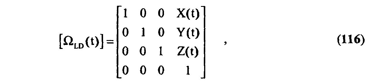
 and
and where (t), ϕ(t) and ψ(t) are the roll, pitch and yaw angles and X(t), Y(t) and Z(t) are the translation components of C VB versus C GB that, together, constitute an expression for the VBPO function.
- Because of the small maximum values of , ϕ and ψ (using the orientations specified above for the coordinate systems C GB and C VB ) their sine and cosine functions may be conveniently substituted in the Ω expression by the truncated expansion series formulas
- The transformation of vectors from the vehicle based coordinates system C VB to the ground based coordinates system C GB may be performed by the use of the formula
- The solution of the VBPO computation problem, which directly yield the solution to transforming vectors from ground based coordinates to vehicle based coordinates and vice versa, consists therefore in the determination of the functions (t), ϕ(t), ψ(t), X(t), Y(t) and Z(t) of time t for a certain vehicle body. In order to do that, an expression must be chosen for each of such functions, which includes a few parameters that can be optimised by minimising a function that expresses the extent of matching between a series of 3DD measurements made on a vehicle and some known features of the relevant rail vehicle model, such features being available from the vehicles database, following the vehicle recognition.
- The VBPO computation will be accomplished by an iterative process starting from initial "guessed values" for the parameters subject to change in the solution finding process. It is apparent that the limitation in the number of parameters to be optimised and an appropriate choice of initial guess values for such parameters are important to converge faster and more reliably to the searched solution. A principal simplification in the VBPO computing problem results from the use of the LDF function, which was computed for the relevant vehicle at the stage of vehicle recognition, as explained above. In fact, under the assumptions made above for the definition of the C VB coordinate system, the function Z(t) may be taken equal to the LDF function L(t). Even though in principle Z(t) could be refined within the VBPO estimation process, the Applicant prefers that it is taken equal to the relevant LDF because this makes the VBPO computing method simpler, faster and more robust. The play of the vehicle body in the Z VB direction vs. the position of wheelsets centres or the position of the bogies rotation axes 261 and 262 is in fact generally very small and thus the use of 3DD data to refine the Z(t) estimation made by the LDF is little useful, if the LDF has been carefully determined by a sufficient number of appropriate wheel sensors and by an appropriate computational method. The choice made of the orientation of the X GB axis allows to consider X(t) as independent of time, unless very accurate 3DD measurements are made. The initial guess X 0 of its value may be derived from the height of the C VB over the rolling surface, which is available from the database. The pitch angle guess value ϕ 0 may be set to zero and this angle could be considered constant, due to its actual low variation for rail vehicles, unless very accurate 3DD measurements are made. The functions Y(t) corresponding to side displacement, (t) corresponding to roll oscillations and ψ(t) corresponding to yaw oscillations are the principal target of the VBPO determination procedure since they are the ones which principally affect the lateral displacement of vehicle body.
- The quantity ζ 2 / VBPO to be minimised for determining the angular and the displacement components of the VBPO function may be expressed by the chi-squared-like formulawhere the quantities ζ r express the extent of position matching of a certain vehicle feature from the vehicles database with one or more 3DD measurement and the σ r values are the corresponding standard deviations. The dependence of the R values ζ r on the parameters to be optimised for defining the VBPO components results from the use of the Ω or the Ω-1 transformation to compute the values of ζ r in the C VB or in the C GB coordinates system.

- The Applicant has considered a few different definitions and corresponding computational methods for the values ζ r and a brief account of some of them is given here below, considering their importance in determining the computational times, the robustness of the method and the implications in the preparation of the relevant features data to be stored in the vehicles database. Such options are related in particular to the choice of the vehicle features, to the measurement system used to obtain the 3DD values and to the definition of ζ r .
- In general, when the VBPO solution search is started by initial guess values for the VBPO components, the corresponding initial error in (t), ϕ(t), ψ(t), X(t), Y(t), i.e. in all VBPO components except for Z(t), is a very important issue to be considered in relation to ζ r definition and computing.
- If the 3DD measurements are performed by one of the means described above using fixed or scanning laser distance meters, the spacing between 3DD measurement directions and the possible gaps between measurements beams can be considered together as a principal limitation in the computation of the ζ r values.
- A first type of vehicle feature that the Applicant recommends to use in this case consists of a flat surface, hereby "large flat feature" or "F1" feature, using the distance of 3DD points from the surface as the definition of ζ r . If more than one 3DD measurement from LDM sensors may be referred to the same flat feature, ζ r may be defined as the square root of the sum of the individual square distances. This feature may be easily coded in the vehicles database by a series of parameters, such as three corners points, defining a rectangle in the C VB coordinates space. A principal advantage of this choice is that one or more corresponding 3DD points can be easily selected by using a surface being long and wide enough to guarantee that such points will refer to the flat surface feature, taking into account the maximum possible error in the initial values of the VBPO components. Some examples of F2 features are a flat portion of the side wall of a wagon, a portion of a flat wagon roof, a flat inclined portion of the upper enclosure of a wagon for transporting coal or a flat plate for mounting labels on a rail chemical tanker. When these flat features are parallel or almost parallel to the X VB Z VB plane, the distance to a 3DD point to be matched will be particularly effective in defining the side displacement Y(t) components of the VBPO function, while the impact on the definition of the roll component (t) will be minimal when the surface height is close to the height of the roll centre and it will increase with the difference between such heights. Its effect on the yaw component ψ(t) will be generally high unless the feature is positioned close to the X VB Y VB plane. When, in turn, the flat features are parallel or almost parallel to the Y VB Z VB plane, the distance to a 3DD point to be matched will be particularly effective in defining the pitch angle ϕ(t) and the vertical displacement X(t) (or just X) components of the VBPO function, while the impact on the definition of the roll component (t) will be minimal when the flat feature is close to the X VB Z VB plane, i.e. close to the vertical of the roll centre, and it will increase with the an increasing side displacement from the X VB Z VB plane. When a flat feature is parallel or almost parallel to the Z VB axis and forms an angle with the X VB axis which is relatively far from all the multiples of π/2 radians, it will generally impact on X(t) and on Y(t) while it will affect (t), ϕ(t) and ψ(t) by an extent that depends on its position over the vehicle. Similar considerations can be made for other orientations of a flat feature, considering that the ζ r is related in this case to the vehicle body position and orientation by a distance that is measured in the orthogonal direction to the surface of the flat feature. The relative importance of a certain flat feature in determining the VBPO components depends of course on the σ r uncertainty referring to ζ r , that must be computed and generally depends on the orientation and on the position of the flat feature.
- A thin and elongated flat surface is a second convenient choice compatible with LDM 3DD measurements, hereby referred to as "thin flat feature" or "F2" feature. This feature, like F1, may be easily coded in the vehicles database are a series of parameters, such as three corners points, defining a rectangle in the C VB coordinates space. This feature is relatively easy to be found also in the important and relatively difficult case of flat rail cars since it may correspond, for instance, to the side surface of parts of the loading deck of the wagon. In this case it is expected that only a fraction of the LDM measurement points which may be selected under the initial uncertainty in the LVPO function will be valid, in the sense of corresponding to a sufficient overlap between the laser beam cross section and the thin surface feature during the measurement, depending on the type of LDM. It is thus convenient in this case that a preliminary processing is made to screen the candidate 3DD measured points. Such screening is particularly easy when the F2 feature has a strong "three-dimensional contrast" with the background, i.e. if a significant distance exists in the direction of the measurement laser beam between the measured distance values at the edges of the feature and the distances of the background. Some types of LDM instruments, particularly the modulation-phase-based ones, will yield widely scattered measurements when the LDM back-reflected light is partially from the edge of the feature and partially from the background and therefore the screening procedure should be able to eliminate 3DD points for which the distance is little higher that the one at the nearest feature edge. Such filtering of the candidate 3DD measured points for an F2 feature may be based, for instance, on the search for 3DD points subsets that fits with a minimum quadratic error a plane whose position and orientation are constrained around the F2 feature position and orientation, the candidate sub-sets elements also being subject to falling within a rectangle which may be seen as the feature itself shrunk by an extent which takes into account the measurement beam cross section size and the orientation of the beam vs. the feature surface. A way to compute ζ r for an F2 feature is the same indicated for the F1, using only the points that were selected by the above screening procedure. An alternate way may be defining the plane that interpolates these points and defining ζ r by the average square distance between the feature and such plane.
- A tile "cut" from a cylindrical surface, hereby called "cylindrical tile feature" or "F3" feature may be a convenient choice for some particular types of freight railcars such as chemical tankers. This feature may be coded in the vehicles database by a few parameters such as the origin and the direction of the cylinder axis plus the cylinder radius and the planes defining the tile or by the coordinates defining the two linear tiles edges and a line parallel to them and lying at equal distances from the two lines or by other manners involving a few parameters defined in such a way to facilitate the calculation of ζ r . The size of the F3 tiles can be assumed large enough to allow the use of the simple way to compute ζ r that is indicated above for the F1 feature. The F3 features are very attractive since, if large enough, they may precisely affect, in the example of a horizontal cylinder, both the VBPO components X(T) and Y(T) at the same time and the (T), ψ(T) components as well, providing that the longitudinal distance of the feature from the X VB Y VB plane is sufficiently large.
- A linear thin solid structure, hereby called "rod-like feature" or "F4" feature is another option compatible with LDM based 3DD measurements. This feature may be used, for instance, for catwalk handrails on rail tankers and for other external horizontal, vertical or inclined features consisting of a pipe and being a fixed component of the vehicle model. This feature may be coded in the vehicles database by two points of the rod axis at it extremities and by the radius of the rod. A pre-processing of the feature data like in the case of the F2 features is advisable and a similar procedure may be used for filtering the candidate 3DD measured points. ζ r may be computed as the square root of the sum of the distances between selected points and the rod surface or defining the line interpolating these points and defining ζ r by the average square distance between the axis of the feature and such line.
- A dihedral structure is another possible feature compatible with LDM 3DD measurements, hereby called "dihedral feature" or "F5" feature. This feature is of very general applicability and may result very useful, like the F2 type, for relatively difficult cases such as flat railcars. Pre-processing of the 3DD data is recommended also in this case by a filtering of the data that results in this case in the classification of the selected points in two groups corresponding to the two dihedral planes. ζ r may be computed in this case as the square root of the sum of the distances between selected points and the relevant surface or defining the dihedral corner line from the interpolation of the two planes and defining ζ r by the average square distance between the axis of the feature and such line. This type of feature is characterised by a relatively complex pre-processing stage but it delivers a ζ r definition which is very powerful in defining at least two of the most critical VBPO components, depending on the orientation and the position of the feature itself.
- A slit in a flat surface is a particular type of feature, hereby called "slit feature" of "F6" feature that may be compatible with LDM based 3DD measurements. This feature may be coded in the vehicle database as the slit width and two end points of its centre line, together with the coding of the relevant surface, as commented for the feature type F1. In this case a filtering of the candidate data points should be done to select the 3DD points which belong to the slit by having measured distances not compatible with the surface and by having three dimensional coordinates and measurement vectors matching the linear slit. ζ r may be defined in this case by the interpolation of the slit centre-line and the computing of the square root of the mean squared distance of this centre-line with the centre line of the feature as coded in the vehicle database. The "discarded" data points which are relative to the surface and separated enough from the slit edges may also be used to define a second ζ r to be computed in the same way of the one for the F1 features.
- A linear thin and low ridge-like structure over a flat surface may also compatible with LDM based 3DD measurements, if they are accurate enough. This structure corresponds to a feature that is hereby indicated as "linear ridge feature" or "F7" feature. The definition, the pre-processing method and the ζ r definitions of are similar to the ones discussed here above for the F6 features.
- A tile cut out of a spherical surface, hereby called "spherical tile feature" or "F8" feature may be a suitable feature for some special cases of railcars when LDM based 3DD measurement are used to define ζ r . The definitions and the methods to pre-process data and to compute ζ r are conceptually similar to the ones applicable to F3 features above.
- Trihedral particulars with sufficiently large plane areas, hereby called "trihedral features" or "F9" features, may be treated as an obvious extension of the F5 features and are an "information rich" option compatible with LDM based 3DD measurements.
- A principal alternative to LDM 3DD measurements for computing the VBPO function is the use of stereo imaging in correspondence to suitable features stored in the vehicles database. In fact, even though the Applicant has expressed above its concern on the robustness of this method for detecting protruding obstacles, it considers such method an interesting option if the feature to be localised in space can be chosen appropriately, as in the case of features stored in the vehicles database. It is of course possible to install additional VIS or NIR imaging sensors with the specific purpose of performing 3DD measurements on selected vehicle features but the Applicant has a preference in using as much as possible for this purpose the same imagers that are installed as discussed above in order to acquire the vehicle images which are used as an input to the OCR processing. Considering the necessity to image contemporarily the features by at least two different imagers for applying the stereo imaging localisation to the vehicle features and being the candidate feature often positioned at the outer positions around the vehicle itself, the increase in the number of line imagers of Fig.10a may be proposed. The use of wider view angles and a higher number of imaging array elements for these imagers is a solution that would allow to avoid a significant increase in the number of line imagers, using the central part of the line images for OCR and documentation purposes and the side parts for stereo image processing, considering that the latter process may tolerate in some cases a lower image quality than OCR does within the Method. A large offset between imagers implies that the definition of the position of the features by stereo imaging becomes a viable option for a limited set of features, including in particular lines and shapes lying on almost flat surfaces. A large imagers offset is however characterised by a higher accuracy in measuring the distance of a feature from the imagers. The installation of a second imager dedicated to stereoscopic vision close an imager devoted to two-dimensional imaging is however an option that may be considered is stereoscopic vision is chosen as a primary method in recognising vehicle features within the procedure to determine the VBPO function components. A different approach to the use of imagers for determining the position of vehicle features in space is the processing of single two-dimensional images (including images constructed by the data from a line imager) containing vehicle features for which one or more dimensional measurements can be made. Using this last method does not generally imply a change in the number of imagers or in their characteristics from what discussed above concerning the imagers of Fig.11a and Fig.11b for OCR and documentation purposes.
- A feature corresponding to the presence of undefined visual signs or markings on a known flat surface will be called herein "flat undefined visual feature" or "F10" feature. This imaging based option can be applied to a number of railcars where markings or drawings are expected on a defined flat area, such as a portion of a side railcar wall. The surface coding indicated above for the F1 features may be used in this case as well. When this feature is used in the VBPO method, a stereoscopic image processing procedure will produce in most cases a localisation in terms of a set of 3DD points defining a surface. The corresponding ζ r value may thus be defined as the square root of the sum of the squared distances of the relevant 3DD points from the feature surface, as for feature F1. Alternatively, the relevant plane in the C GB space may be defined by the image processing results and the square root of the squared average distance of such plane for the relevant surface defined in the vehicle database may be used as a ζ r definition
- A visual shape with known dimensions and unknown exact position on a flat surface will be called hereby "floating fixed-size shape" or "F11". The processing of the relevant image or images may be done in this case by stereo or single imager methods, thanks to the known absolute dimensions of the shape. The image processing results locate the relevant plane in the C GB space and the square root of the squared average distance of such plane for the relevant surface defined in the vehicle database may be used as a ζ r definition.
- If a visual shape on a vehicle plane surface has a defined dimension and a defined orientation and position, it will correspond to a "wholly defined shape" or "F12". The processing of the relevant image or images may be done in this case by stereo or single imager methods, and the image processing results may be used in the case to compute ζ r as the square root of the squared average distances between the two shapes which are defined by the measurements and by the relevant coding in the vehicles database.
- Not all the above-indicated types of features must necessarily be implemented in a System embodiment. Other types of features may be defined together with their coding in the vehicles database and one or more methods to compute one or more ζ r values. The methods for the quantification of the uncertainties σ r for the ζ r values are not discussed here because they would take several lines of text and because they may be defined without major difficulties by those skilled in the relevant art, such as experts in numerical computing for robotics.
- More than one type of feature will be used in general for a certain vehicle model in the vehicles database and the choice of features will be done by a set of different criteria with the goal of maximising the performance of the VBPO procedure while limiting the complexity and the cost of populating the vehicles database. The applicability of a certain feature obviously depends on the geometrical characteristics and on the operational features of individual vehicles and is conditioned by the type and position of the sensors that are installed in the System implementation and on their position and orientation. In case more than one version of the System are implemented (with different instruments types and/or positioning) the vehicles database may exist in a single version and contain features that are applicable only by some of such versions. A series of basic criteria are defined here below to decide which features should be better uses when defining the vehicle database contents for a certain vehicle, without implying that their sequential order corresponds to their relative importance neither that other criteria at least as important as some of them do not exist.
- An obvious but fundamental criterion for choosing the positions and the size of the vehicles features for a vehicle model is the avoidance of interferences from the load and particularly from the presence of imaginable abnormal loads and of the possible excessively protruding items that would be detected by the System. This criterion should not however be taken as imperative for all features and it should be disregarded if it clashes with the possibility to define enough well-chosen features according to the other criteria here below.
- The different types of features have a different impact on the fitting of the (t), ϕ(t), ψ(t), X(t) and
- Y(t) functions, also depending on the features positions. The types and positions of the chosen features should be therefore such to avoid a lack of a determination for each of the VBPO components and particularly for the more critical ones.
- The (t), ϕ(t), ψ(t), X(t) and Y(t) functions will be fitted by measurements carried out at a series of times with corresponding different displacements of the vehicle versus the ground based instruments. The choice of the features and of their position on the vehicle should therefore consider the interval between the features and the positioning of the instruments in order to get a sufficiently even distribution of sensed features in the vehicle scanning for an effective determination of time-dependent VBPO components, with special reference to the more critical ones.
- The twelve types of features discussed above are clearly characterised by a diverse complexity and a diverse extent in using computing resources. The required runtime computational resources should therefore be considered, taking into account that some of the computations, particularly the ones called pre-processing while commenting the various features, are carried out only ones whilst the ζ r values are computed several times in the minimisation of expression 125.
- The computation of the VBPO function should be taken into account also while deciding the longitudinal positioning of sensors around the track, especially in relation to the performance of the gauge and thermal diagnostic methods for the vehicle body. A first consideration about this issue is that the computing of the VBPO and particularly of the ϕ(t), ψ(t), X(t) and Y(t) components by the measurements indicated above requires that appropriate 3DD data are available at adequately short time differences for at least two locations with a sufficient longitudinal spacing. A second consideration is that, similarly to what discussed above about the positioning of wheel sensors in relation to the SMI, it is important in this case that the three-dimensional position and the orientation of the vehicle body is known with a sufficient accuracy when a gauge related or a thermal detection measurement is made, taking into account the time difference or the longitudinal displacement between the measurements used to compute the VBPO and the measurements to be associated to the vehicle components by the Ω or the Ω-1 transformation.
- As discussed further below, the use of 3DD measurements for the gauge related functions requires that they are repeated at least twice to reject false alarms from flying interfering items and it was commented above that the sensors positioned in the SMI for detecting 3DD data for the two lateral sides of the vehicle body should be conveniently displaced in the longitudinal direction. Therefore, an advantageous location of the relevant 3DD measurements sensors may be an almost equal spacing along the SMI, alternating their installation on the two track sides and with a sufficient distance between their two extreme positions in relation to the positions of the sensors for the gauge and the thermal diagnostic functions, such sensors being in part coincident with the sensors used to compute the VBPO.
- As in the case discussed above of the LDF functions, the VBPO functions, an particularly of the (t), ψ(t) and Y(t) and Z(t) functions, may be fitted using cubic spline functions. In such a case, the number of spline pieces and their constraints should depend on the train speed and should be consistent with the actual dynamics of railcars, using worst case assumptions or, possibly, some parameters from the vehicle database. The use of truncated Fourier series or their combination with spline functions could be an alternative, with special reference to the rotational VBPO components.
- Standard multi-parameters optimisation techniques may be used for the VBPO definition by the minimisation of expression 125. A choice is however left about computing the ζ r in the C GB or in the C GB coordinates spaces, correspondingly applying the Ω transformation of the 3DD measurements or the Ω-1 transformation on the vehicle features coordinates. The second choice may be advantageous if the feature is described by a few vectorial parameters while the relevant 3DD measurements related vectors are many.
- Because of the possibility that the measurement of a feature is disturbed, particularly by a normal or abnormal load item, the VBPO computational procedure should be such that, at least in the presence of convergence problems, the computation is repeated neglecting one or more of the considered features until a satisfactory convergence is achieved. The failure to achieve a satisfactory convergence of the VBPO computational procedure would result in the generation of an error flag or message to be dealt with appropriately by the other functions applicable to the relevant vehicle.
- The method corresponding to box 237 of Fig.3 is described here below to detect the presence of gauge-related hazards for a rail vehicle whose model has been identified and for which the VBPO function components have been computed as discussed above. The relevant gauge-related hazards include gauge-incompatible vehicles, protruding structures from faulty vehicles, inadmissible load profiles due to inappropriate loading or to load shifting and irregular loading. This method does not apply to the lower parts of the vehicle, as defined by UIC 505 series leaflets [050, 051, 052], such parts being the subject of a different discussion further below in this document.
- Fig.15 a is similar to Fig. 5 of UIC leaflet 505-1 [050] and includes some profiles and parameters that are referenced to in the discussion here below concerning the detection of gauge-related hazards for the vehicle body and its load. The Applicant clarifies that the following comments to Fig.15a, alike the comments to Fig.15b further below, are not meant to be an authentic and comprehensive interpretation of the relevant contents of the UIC code and they purely have the scope of supporting the reading and the understanding of this section of the present document, under the assumption that the reader has a sufficient familiarity with the UIC 505 series of leaflets. The two axes 560 and 561 define the "normal coordinates" system for a track and a vehicle transversal section perpendicular to the longitudinal track centre axis. These normal coordinates, used in the UIC 505 leaflets series, are common to both the vehicle and the way under the assumption that the vehicle is stationary and it is symmetrically positioned with its vertical axis passing through the local track centre axis. The origin of both axes 560 and 561 lay on the rolling surface at equal distance from the rails. The whole subject of rail vehicle gauge according to the UIC code is based on the adoption of a certain gauge which comprises a reference profile and a set of rules that, taking such profile as a common basis, allow the rolling stock services to define a maximum allowable profile for the vehicles (and their load) and the way and works services to define the limiting profile for the infrastructure elements. The various profiles 562, 563, 564, 571, 572 and 574 are defined in the UIC 505 leaflets series in correspondence to a classification of the effects of a number of factors such as the position of the vehicle body parts vs. the rails at a curve, the inclination of the vehicle around its rolling centre, the lateral displacement of the whole vehicle body due to cant deficiency or excess, the wear of vehicle and rails, the mechanical plays between some parts of a vehicle, the kinematics of bogies and axles, the imperfections of the track, the subsidence of rails and sleepers in the ballast, etc. The profile 562 corresponds to the limiting vehicle construction gauge profile and it defines the maximum offset positions from the axis 560 of any vehicle part (at a certain longitudinal position along the vehicle). The profile 563 corresponds to the reference contour of the kinematic vehicle gauge and the E distance 566 between this contour and the vehicle construction profile 562 is given by the "reductions" to be evaluated according to rules given in the UIC 505-1 leaflet [050]. The quantity E is actually corresponding to either E i or E a depending on the position of the relevant transversal section being between the first and the last axles not mounted on bogies or between the bogies castings or being outside such positions interval. The z component of E is the "quasi-static lateral displacement" which accounts for the side inclination resulting from the component of the vehicle dissymmetry angle exceeding one degree and from part of the effect of an excessive or deficient cant. The profile 564 corresponds to the outer limit of any part of a vehicle as considered by the reduction formulas. The profile 564 is separated from the profile 563 by the distance S or "lateral projection" 567 and differs from the profile 562 by D, which is the distance corresponding to the overall lateral displacement 568. S is the quantity by which the vehicle contour exceeds the reference profile when it transits on a curve and/or the rail gauge exceeds 1435 mm (for the standard rails gauge). The half width of the vehicle profile at a certain height plus the quantity D and minus the half width of the reference profile at that same height is equal to the effective value of S, relative to the reference profile. The reductions E i or E a must be equal or greater than the quantity D-S 0 , where S 0 is the maximum value of S, to exclude that any part of the vehicle is positioned outside the vehicle position limiting profile. The profile 571 corresponds to the vehicle kinematic obstruction profile and its half width exceeds the half width of profile 564 by a distance 569, which is the part of quasi-static displacement that is not accounted for within D. The profile 572 corresponds to the limiting positions of any way-based part and is separated from profile 571 by the distance 570, which accounts for the oscillations and the dissymmetry below one degree and reflects the lateral displacements resulting from the imperfections of the track. The profile 573 corresponds to the actual limiting physical contour of the infrastructure and its half width exceeds the profile 572 by the distance 574, which is chosen for a certain track taking into account special operations or situations such as the transport of wide and/or very long loads or the frequent occurrence of very strong side winds. The vehicle limit position profile 564 separates the competences of the rolling stock services from the ones of the way and works services, which are responsible for the clearances belonging to the dashed area of Fig.15 a.
- A principal issue which is considered in this invention is that the allowed vehicle profiles 562, i.e. its maximum allowed width at a certain height over the rolling surface, depends on the distance between the relevant transversal section and the bogies castings or the two extreme fixed axles. This follows from the fact that the reductions of the vehicle versus the reference gauge profile include the "geometrical lateral offset" of the vehicle body for a radius of the rail curvature equal or exceeding 250 metres, the extra side clearance for lower curvature radius being taken into account in determining the required gap between the infrastructure profile and the vehicle position limiting profile. Fig.15 b shows, similarly to Fig. 4 of UIC leaflet 505-1 [050], an horizontal section of a vehicle with the different parts 577, 583 and 582 of the profile of the maximum construction width of a vehicle, such profile being significantly influenced by the geometrical lateral offset depending on the position of a transversal section along the longitudinal axis 575. In practice, most vehicles have a construction profile 585 corresponding to the dashed area 580 that consists in a rectangle contained within the maximum allowable profile, mostly because of the implications of the geometry of stations platforms and other structures, with a bevel 576 at the four corners.
- The UIC code leaflets concerning the vehicles and the infrastructure profiles are of course setting profiles limits on the vehicles loads as well and they are also used for the case of extraordinary loads on wagons. The profiles of loads are however the subject of further norms such as, where applicable, the vehicle loading prescriptions in the RIV Agreement [060] and its Annexes. Particularly, Part 4, Volume I, Annex II of the RIV Agreement indicates a series of transversal contours limits for loads, based on a set of "Loading Gauge Profiles", which are subject to reductions indicated in a set of relevant tables. In the same section other loads geometry limits are indicated concerning the longitudinal extreme load positions and about the use of composite, multiple and articulated wagons.
- Part 5 of the RIV Agreement [060] (as well as UIC leaflet 502 [075]) addresses the coding and the labelling of exceptional loads, the corresponding coding of rail lines and the rules to apply such coding to allow the safe transportation of such exceptional loads. The coded exceptional loading profiles also constitute a type of profile that may be used by the System. UIC leaflets 596-5, 596-6 and 597 [054, 055, 056] address the profiles for combined rail transport. The System can use these profiles as well within its functions to detect gauge-related hazards. In the case of combined transport and in the case of the transport of extraordinary loads (called "special consignments" in the UIC 502 leaflet [075] and elsewhere) the System may read, by OCR and OCR-like processing of the images of a vehicle, the special markings that the relevant norms define. The reading of such markings allows the System to determine which particular profiles should be used to detect violations of the combined transport profiles or of the extraordinary loads profiles.
- The detection of loading profile violation but not of the maximum admissible profile for the vehicle and its load may be the indication of an item which has displaced from its correct position and which could further displace at a later time, up to becoming a gauge-related hazard.
- In addition to the UIC construction profiles and to the loading profiles, it may result useful in the application of this invention to consider the actual construction profiles of wagons because, for instance, the system could detect, if desired, the presence of abnormal items within the admissible vehicle profile, e.g. a clandestine passenger laid at a free side space beneath the tank of a liquid chemicals transport railcar.
- Fig.16 will be used here below to address a method to detect the presence of an item beyond a certain relevant profile integral to a passing vehicle. Such certain relevant profile can be the admissible construction and loading profile according to the relevant UIC 505-5 [052] principles or it can be a construction profile known from the vehicles database or it can be a standard loading profile or a coded profile for exceptional loads of for combined transport (e.g. according to the relevant annexes of the RIV Agreement [060] and/or to UIC leaflets 596-5, 596-6 and 597 [054, 055, 056]). The axes 601, 602 and 603 correspond to the C GB ground based coordinates space with origin in 600 while the axes 605, 606 and 607 pertain to the C VB vehicle based coordinates space with origin in 604. C GB and C VB are the same coordinates systems discussed above while commenting Fig.14, despite the differences in their mutual positions and orientation, the relative rotation of π radians around the X axis of one of the two coordinates systems resulting from a different train transit direction between Fig.16 and Fig.14. Reference numbers 608 to 612 indicate half of five profiles defined over different transversal vehicle sections corresponding to different values of the longitudinal vehicle coordinate Z VB , indicated by the intersections, marked by a thick dot, of the profiles vertical axis with the Z VB axis. These profiles may generically correspond to vehicle sections such as 578 and 581 in Fig.15 b or to other profiles mentioned above. Box 614 represents a distance measurement optical device that provides a measurement for the position of a point M, indicated by 617, at the surface of what can be supposed to be a vehicle-based item. 616 indicates the measured vector originated from a position 615 at the measurement instrument, defined by the coordinates values 618, 619 and 620 referring to the C GB axes. The coordinates transformation operator Ω, whose parameters vs. time were computed for the vehicle as discussed above, is used by equation 113 to define the position of M by the values 621, 622 and 623 in the C VB coordinates system. Ω may also be applied to convert to the C VB coordinates system the measurement versor, which can be used to estimate the relevant position measurement uncertainties in different directions. The comparison can thus be made between the position 616 of point M and the envelope defined by a set of limiting profiles in the same coordinates system C VB . It is however apparent to those skilled in the art that the computations related to the detection of items beyond certain vehicle profiles can be alternatively made in the C GB coordinates system by the use of the Ω-1 transformation applied to the relevant vehicle profiles, which are defined in the C VB coordinates space.
- Any type of pre-defined vehicle-based profile for detecting items in profile-violating positions may be stored in the vehicles database using an appropriate longitudinal pitch, such as 613 and the limiting distance to compare the detected position 616 may be then be interpolated from the distances 624 and 625, or by more such distances to take nonlinearity into account, at the relevant height from the nearest profiles 610 and 611. The pitch distance 613 may be defined as a fixed value or it may depend on the longitudinal position and it should be ideally chosen taking into account the first and second derivatives of the profile width versus z VB . An obvious alternate way to define a profile is by the use of a series of profile lines corresponding to horizontal (instead of vertical) surfaces. Alternatively the vehicle-based profiles may be stored as a set of surfaces or may be computed using parameters and appropriate formulas, with special reference to the methods described in the UIC vehicle gauge related leaflets 505-1 and 506. It should be recognized, in this respect, that the accurate computation of the admissible profiles for a vehicle requires some input parameters, e.g. the flexibility coefficient, that can be stored in the vehicle database for each of known vehicle models and that are awkward to derive from any measurement that can be made within the SMI. The loading profiles that are defined as mentioned above by the standardised markings on the vehicles for combined transport and for the transport of extraordinary loads are stored at the system in one of the means defined here above and they are retrieved according to the result of the OCR and OCR-like reading by the System of such markings.
- The criterion for considering a single detected position M as a profile violation in terms of vehicle or load width can be defined by the condition
- The expression
- A further term ξ (actually ξ y or ξ x ) may be further added to the left expressions of 126 and 127, particularly for the case in which the relevant profile is the admissible profile according to the principles of UIC 505-5 [052], leading to the conditions
- Depending on the type, the performance and the installation geometry of the instruments, the generation of gauge related alarms and warning messages can be conditioned to the detection of two or more points M forming a small cluster. In such a case, the expressions 126 and 127 (or 128 and 129) can be used to select each of such points and diverse conditions can be defined considering all the elements of such a cluster in order to reduce false alarms. A particular condition that may be applied to reduce the rate of false alarms, depending on the suitability of the 3DD measurement systems, is the presence of nearby intermediate M points from the outer inadmissible M positions towards a set of M points inside the admissible space, in order to exclude small flying items such as single leaves or small paper clips.
- A principal mean to reduce the false alarms rate is requiring that an alarm is consistently generated by the processing of 3DD data for two or more different positions along the track, as suggested, for instance, in 004. The consistence criterion for the subsequent detections typically requires in the case of this invention that the possible hazardous or abnormal item has moved almost integral with the vehicle. This alarms filtering technique may imply a considerable additional cost of the System hardware if its implementation requires the installation in the SMI of additional expensive measurement instruments but this may not be the case if the installation of such instruments is anyway justified by the use of their measurements to compute the Ω parameters. Furthermore, it is generally possible that the successive detections are based on 3DD measurement carried out by different types of instruments. This technique is very effective to suppress a significant fraction of the possible spurious gauge-related alarms and it can be implemented with ease and with a modest development effort in the relevant software. A special group of a gauge-related hazards is the one of loose or torn wagons sheets and of covering or wrapping sheets of individual loads over open wagons because in these cases the detected clusters of 3DD points could significantly float between two successive detections in the SMI. Even though it is possible to implement some alternate methods with a good statistical performance in recognising these cases and discriminating them from a flying shopping bag or plastic sheets, the Applicant considers advisable that such discrimination is made by a remote operator, as discussed further below.
- The detection of gauge-related hazards for a certain rail vehicle requires that the relevant set of 3DD measurements is retrieved from the whole set of 3DD measurements. Such data fetching process can be performed by calculating a measurement time range for each 3DD measurement instrument, taking into account its installation geometry, its calibration parameters, the Ω coordinates transformation operator (or the LDF) and a small margin, ideally computed as a function of the velocity of the vehicle during its transit across the SMI. Even though the whole process of comparing the 3DD points can be performed in the C VB coordinates space, it may result advantageous that a selection of those 3DD points that may correspond to hazardous items is first carried out in the in the C GB coordinates space using a "conservative" profile.
- The acceptability of a certain vehicle and load limiting profile according to the principles of UIC 505-5 norm is related to the actual or the assumed obstacles profile along the train itinerary and on the velocity at which the train will travel. In order to exploit the System usefulness for the widest possible range of installations, it is therefore advisable that the System software is designed and developed in such a way that it can efficiently perform the gauge related diagnostics for a set of different alarm conditions (with particular reference to conditions 128 and 129) corresponding to different infrastructure contours and to different train speed values.
- The techniques described above to detect gauge-related hazards lend themselves to be used in a number of possible ways depending on which profile definition is used and on how the System exchanges information and messages with certain railway information systems or manned control centres. Some possibilities are non-exhaustively discussed here below concerning the generation and the management of gauge related diagnostic messages, alarms and data.
- The detection by the System according to the principles of UIC leaflet 505-5 [052] of the "incompatibility" between a vehicle profile, including load when applicable, and the infrastructure profile, taking the term ξ into account if appropriate and possible, should result in the generation of a gauge alarm that should be sent, directly or indirectly, to the signalling system of the railway in order to stop the train at the first convenient position or to redirect it to a safe branch.
- An alarm should be sent, directly or indirectly, to the signalling system of the railway (in order to stop the train at the first convenient position or to redirect it to a safe branch) also when the violation is detected of a loading profile of the following types:
- loading profiles defined by the RIV agreement [060] for loads charged on ordinary flat and open wagons;

-
-
-
- Such detected loading profile violations are in fact likely to be associated to the presence of a shifted load or to an improperly charged load.
- Of course, the recognition of a special loading profile by the coded marking on a vehicle or its load in association with detecting no violation for that load can be used by the system to suppress a possible alarm or warning message in relation to the violation of loading profiles defined by the RIV agreement [060] for loads charged on ordinary flat and open wagons. In this way the System will avoid the generation of a number of spurious alarms and warning messages in correspondence with special consignments.
- In general it is possible to define two or more tolerance limits for comparing the 3DD data with profiles and to send a warning message (plus data & information) instead of an alarm when the stricter tolerance values correspond to a violation (whilst the broader value does not). A balancing of sensitivity and spurious alarms rate can be achieved in this way in order to safeguard the risk reduction level associated with the use of the System without compromising the railway operations. In any case of profile violation (maximum admissible profiles, loading profiles and construction profiles) it is possible and advisable to dispatch a warning message to a control centre, together with data and information that may allow a remote operator and/or a software application to evaluate the case and take an appropriate action (e.g. sending an alarm to a safety and signalling system, sensing a message to the relevant train driver/crew or suppressing an alarm generated by the System and already sent to safety and signalling system).
- It is also possible that the generation by the System of alarms and/or warning messages is suppressed if the System has received from a railway system the information that a certain gauge-related abnormal situation is known (e.g. that a relevant vehicle is intentionally loaded beyond its standard loading gauge).
- It is advisable that, if an information data set has been received by the System for the relevant train including the train itinerary along a series of track stretches with certain infrastructure profiles and/or a reduced velocity schedule, the System takes such information into account in order to conduct the gauge-related hazards detection functions appropriately.
- It is also possible that the System sends to a railway information system a gauge profiles data set for all the vehicles that were found to have a violation of their loading gauge or a violation of a certain minimum gauge profile (e.g. the one corresponding to the standard reference gauge of UIC leaflet 505-1) and that the railway information systems use such data set to perform a compatibility check immediately or later, depending on the actual itinerary followed by the train. In this case the data set can contain profile data for the vehicle and its load or may consist of a compatibility flag for a series of infrastructure profiles known to the System, possibly as a function of the vehicle speed.
- A series of specific diagnostics methods can also be implemented to recognise the violations of the RIV or of certain other loading rules that cannot be strictly classified as gauge-related. An example of such a violation is an insufficient longitudinal distance between two loads on two different adjacent rail vehicles with the first load extending from the vehicle it is loaded on to the second vehicle, e.g. with reference to loading directive 4.3 in Part 4, Volume I, Annex II of the RIV Agreement [060]. Such methods would have in common with the gauge-related diagnostics discussed in this section of this text the use of information related to the rail vehicle model and the application of the Ω or Ω-1 operators to refer any measurement made to a point, or to an origin and a direction, relative to the vehicle.
- Different types and models of rail vehicles have a different probability of presenting gauge hazards, e.g. in relation to the possibility of improper loading or load shifting, and it is therefore advisable to perform the analysis of the more risky vehicles before the less risky ones, in order to minimize the average time to signal important gauge related hazards.
- Even though the System can apply the gauge-related diagnostic functions on any rail vehicle, it may be decided that certain entire groups of identified railcars, particularly passenger cars, are not checked. It is however advisable that a basic gauge compatibility verification is applied for all vehicles, checking that their model has been approved for circulation on a line characterised by the relevant reference gauge. This basic check may be particularly indicated if the vehicles database has not been fully populated yet and the full data sets for the vehicles with a higher risk of presenting gauge-related hazards are being provided and/or coded with a higher priority.
- The detection of gauge-related hazards for the lower parts of a vehicle is dealt with here below, separately from the former discussion for the vehicle body, in accordance to the separation of the discussion for the low and high parts of vehicles in the UIC 505 leaflets. Furthermore this separate discussion of the lower vehicle parts profile diagnostics is justified because of the different risk and of the different implications in terms of measurements instruments to be installed at the SMI.
- Even though 3DD measurement instruments may be selected and installed for the lower vehicle parts using design principles similar to the ones discussed above for the 3DD measurement related to the upper vehicle parts, doing it for the lower parts presents some additional difficulty. Such instruments should be in fact positioned close or below the rolling surface and have their front optics or windows looking horizontally or at higher elevation angles, with the known problems related to the protection from dirt, projected gravel pieces, weather agents in the presence of a strong air turbulence, grease, etc. Additionally, the 3DD measurement instruments should be compatible with the track vibrations or installed with an appropriate decoupling from them and they could necessitate special care or re-installation during the track maintenance operations. The Applicant does not however consider such difficulties as a problem requiring innovative solutions since, even for the "worst case positioning" those skilled in the art may apply some of several alternate technical solutions that were adopted to date for "hot box detectors" (e.g. protecting lids opening during measurements, housing in hollow sleepers, clamping systems for attachment to rails, vibration dumping for delicate components, etc.). These possible inconveniences concerning development, installation and operation may however contribute to the decision of implementing the System without the measurement instruments required for detecting the presence of gauge-related hazards for the lower part of vehicles.
- In case the System implemented functions comprise the detection of gauge-related hazards for the lower parts of a vehicle, the computational methods to accomplish that are essentially the same that have been exposed above for the upper vehicle parts. The detection of gauge-related hazards for the lower parts of a vehicle would additionally take into account the UIC 505 issues related to the admissibility of vehicles over humps at gravity yards.
- The text here below addresses the functions, corresponding to box 239 of Fig.3, for the detection of a series of abnormal conditions and defects for axles bearings, wheels and brakes, based on infrared passive sensing, for those vehicles whose model has been positively identified.
- Consistently with the data processing method that is addressed below and with its possible details variations, more than one type of infrared sensing apparatus or combination of apparata possess the minimum relevant requirements in terms of spatial coverage, instantaneous field of view for a single pixel or sensor, accuracy and measurement rate. A review is thus made here below of some alternate options concerning the apparata or set of apparata (hereby indicated by "BWBTIS" for Bearings, Wheels and Brakes Thermal Infrared Sensors") that can be integrated within the System to perform the measurements that allow the System software to detect a series of abnormal conditions and defects for axles bearings, wheels and brakes. The Applicant points out that this review is intentionally concise because many of the relevant matters form the subject of a number of prior patent documents, particularly within the IPC class B61K9/06, such as patent documents [005, 008, 016, 018, 019, 026] and some of patent documents cited therein.
- A first group of BWBTIS employs a single infrared detector or a few detectors with the appropriate optics, electronics and mechanics allowing their mounting close to the rails or attached to a rail or inside a hollow sleeper. The use of different types of sensing elements was disclosed, including in particular thermistor bolometers, LiTaO3 pyroelectric sensors, PbS and PbSe photoresistive detectors, HgCdTe (MCT) and InSb photons detectors. Diverse technical solutions have been implemented in such devices to compensate for temperature change, to recalibrate the thermal radiation measurement and to provide in some cases a signal that refers to the difference between the temperature of the observed target and ambient temperature. Many of the commercially available devices of this group are provided with automatic lids protecting the optics when sensing is idle and with heating devices to cope with snowing and freezing. A significant part of the electronics for these systems and of the inventions made in the specific field are related to the analog and/or digital processing of the infrared detectors signals in order to increase the sensitivity and reduce the false alarms rate. The System is however largely independent on such ancillary electronics or data processing methods. The signal processing electronics for these products is generally mounted with the sensors or in separate signal evaluation and signalling units (in this case the sensing device is generally called "HBD scanner" while the signal processing and signalling unit is often called "detector"). Some commercial devices of this group may be interfaced to the System in different ways, possibly with some modifications, with the only fundamental requirement of acquiring the thermal detectors signals with a sufficient resolution, measurement rate and accurate timing in such a way that the System software can associate each measurement to a time that may be accurately referred to the times at which measurements are made by the other sensors and instruments installed at the SMI. Other signals from these devices, e.g. related to calibration and diagnostics may be acquired by the System if convenient and appropriate. The control of the BWBTIS devices of this group, including for instance the opening and closing of protecting lids, temperature control and calibration shutters, may be transferred in part to the System software by the use of an appropriate hardware interfacing or may be left to the electronics of the devices. The choice of the extent of the possible modifications required to these devices in order to integrate them with the System will generally depend on economic considerations, taking into account development, industrialisation, production and maintenance. An example of a commercial BWBTIS of this group is the scanner unit of the "Sentry System" by Southern Technologies Corporation [962], which is used to aim to axles boxes or to wheels, depending on the installation mean. General Electric Transportation Systems [963] offers a range of BWBTIS devices of this first type that may be integrated in the System, including the "ACS" ("Advanced Concept Scanner"), the "VLS" ("Vertical Look Scanner), the "HWD" ("Hot Wheel Detector") and the "FUS" ("High End Hot Box Detection").
- A second group of BWBTIS devices suitable for integration in the System consists of one or a few fast infrared sensors, i.e. photon detectors, with a mirror scanning system that steers the sensing beam in a plane or close to a plane that is orthogonal to the vehicles motion direction. Devices of this type ("VAE-HOA/FOA 400") are available from VAE Eisenbahnsysteme [964] in a few different versions, including alternate mounting options. Depending on the scanner mounting, these scanning detectors monitor axle bearings from either sides of the wheels, the axle itself, the wheels and the discs of brakes, if present.
- A third group of BWBTIS devices corresponds to linear infrared imagers based on infrared sensors linear arrays. These imagers pertain to the group as "staring arrays" imagers (a denomination widely used in the relevant open literature), as opposite to the fast scanning photon detection devices. These devices, mounted with their viewing plane vertical or almost vertical, produce a series of line images with the advantages of a much wider continuous or quasi-continuous spatial coverage vs. the devices of the first group above and of relatively small sensing spots on the measured targets, corresponding to each pixel of the array. Fig.17 a and Fig.16 b show two idealized views of a linear infrared imager installed close to one rail 655 or 658 in order to perform thermal emission measurements for different parts of wheels, bearings and brakes pertaining to an axle 645 or 633. The viewing plane of the linear infrared imager 650 or 638 is vertical or almost vertical, even though it could be inclined if convenient. The imager has a field of view corresponding to angle 647 between the viewing directions 660 and 648 corresponding to the two extreme used pixels of the linear sensors array. The central view direction 652 bifurcates angle 647 in two equal parts and it defines a relative elevation angle 651 versus the rolling surface plane 649.
- The observation of items such as the disc brakes requires a sufficient "slant" angle 635 between the viewing plane and the normal 636 to the track axis. The measurement optical beam 637 coincides with beam 646 while the lines 639, 640 and 641 represent viewing planes or beams at different times vs. the time for which the axle longitudinal position corresponds to the measurement beam 637. A measurement such as the one of beam 646 or 637 corresponds to an angle 653, depending on the relevant pixel and on the positioning of the imager, and to a time value. Such angle could be of course measured relative to another viewing direction, such as for instance the central beam 652.
- The possibility to perform measurements of different items clearly depends on the position of the imager, on its view angle 647, on the elevation and slant angles 651 and 635 and to the possible inclination of the viewing plane versus the rolling surface. In general, at least two imagers are required to observe both wheels of an axle and all brakes discs. The positioning for each side of the track of two imagers with opposite angles 635 could have some advantages in terms of visibility of the targets and to take into account the temperature differences between the leading and trailing faces or items such as bearings but is generally not a requirement. The longitudinal pitch 642 between two successive measurements for the same pixels of the linear infrared sensors array corresponding to view adjacent beams or planes 640 and 641 is of course a fundamental figure of merit, with particular reference to the detection of overheating for relative small items such as bearing 630 and 654. Depending on the particular type of linear infrared imagers, the pixels of the linear array will perform their measurements synchronously or sequentially. It is also possible that the pixels are not disposed along a straight line but on two or more parallel lines and in such a case they will be associated to different slanting angles, to be considered in data acquisition and processing hardware and/or software.
- Very few options are practically available for the choice of infrared sensor linear arrays because a relatively fast response time is required due to the vehicles speed and because the use of high-cost sensors and/or of low-temperature cooling systems are two principal negative elements for the System implementation. In fact, while the number of pixels required for this application in order to achieve the desired spatial resolution depends on the viewing distance and on the optics field of view, the longitudinal resolution (i.e. in the direction of the vehicle movement) is limited by the response time of the array sensors. A vehicle at 120 km/h displaces longitudinally (distance 642 of Fig.17 b) by about 33 mm (or 22 mm at 80 km/h) and it is thus clear that the suitable sensors should have a response time at least in the order of 10-3 s to avoid blurring in the direction of motion and to allow an appropriate longitudinal measurement pitch, as mentioned above. The requirement of a short response time excludes from the choice the most popular and widely available type of uncooled staring arrays, i.e. the thermistor bolometers arrays, whose response time [068] is far too slow. As pointed out by Yaktine et al. [026], two types of fast infrared arrays that may be considered as particularly attractive for this application are the "microthermopile" arrays and the photo-conductive sensors arrays, particularly the PbSe ones since the shorter wavelengths sensitivity of PbS sensors (about 1 to 3 µm vs. about 2 to 5 µm for PbSe, with a dependence on the sensors temperature) makes them less suitable for the targets temperature range of interest.
- Honeywell Inc. (Plymouth, MN, USA) [069] developed the technology for the fabrication of microthermopiles arrays, or "thermoelectric arrays", as a silicon monolithic structure with silicon nitride bridges supporting the hot thermoelectric junctions over micro-wells etched in the silicon substrate [068] and with the corresponding cold junctions close to the rim of the micro-wells. A "speed optimised" 96 pixels array of this type with 150 by 150 µm sensors was used by ISI (Plymouth, MN, USA) [068] to develop the "Model IR 1000" high-speed imaging radiometer. The "Model IR 1000" pixels were designed [068] for a thermal response time of 7.5 10-4 s so that high speed operation is achieved by sampling the signals for 8 10-4 s, with an array scanning rate of 103 s-1. The sensors spectral range (8-12 µm) is particularly indicated to perform thermographic measurements at relatively low temperatures over ambient and to reduce the sensitivity to reflected and diffused sun radiation. NETD (Noise Equivalent Temperature Difference) with an f/0.8 germanium lens is about 0.7 K for room temperature targets and the measurement range extends from about 30 to over 400 degrees Celsius with a short-term accuracy of about ± 4 degrees Celsius or 2%. Two principal advantages of this type of instrument for this application are room temperature operation without any kind of cooler for the sensing array and a good stability over time. Not requiring a chopper reduces cost and maintenance. Moreover, the absence of a chopper allows the implementation of an internal or an external sampling trigger. An excellent account of the characteristics of this device and a description of its use to acquire thermal images of rail vehicles wheels and bearing boxes may be found in a patent document [026] by Yaktine et al. of SAIC (Science Applications International Corporation, San Diego, CA, USA).
- Photoconductive PbSe linear arrays provide for this application a sufficient infrared responsivity at thermoelectrically coolers temperatures in the 2-5 µm wavelengths band with a bandwidth that is well in excess of 104 s-1. A few different manufacturers provide packaged PbSe arrays, with or without multiplexers and amplifiers, which can be integrated in order to provide a linear imaging infrared device. An example of such products is the M-2105 Series by Northrop Grumman Electro-Optics Systems of Tempe, AZ, USA, including a 128 in-line elements array with 91 by 102 µm pixels and a 256 elements bi-linear array with staggered 38 by 56 µm pixels. Even though photoconductive detectors may be read-out in DC or AC modes, with or without a fast comparison with a reference target, the very high dependence of the pixels resistance from the pixel temperature requires for quantitative measurement applications the use of choppers, which generally limit the array scan rate to about 2 103 s-1, which is however compatible with the present application. NETD values below 1 K may be achieved for target temperatures in excess of a few tens of degrees Celsius using f/1.0 or better silicon lenses. The control and/or the measurement of the temperature of chopper and of the other parts of the imager affecting the measurement allow to obtain an adequate accuracy over time for this application. These sensors arrays are therefore providing an alternative to the thermoelectric arrays discussed above with the main advantages of a high pixels number and a fast response time but with the principal disadvantages of practically necessitating a chopper and of requiring a thermoelectric cooler.
- Other types of linear infrared sensors arrays are however not to be excluded for this application, such as for instance the MCT arrays used in the design disclosed in patent document [019] or the few elements LiTaO3 arrays mentioned in patent document [018].
- FPA (Focal Plane Arrays) thermal imagers could also be used, as suggested for instance in some prior patent documents [003, 004], and constitute a fourth BWBTIS group. The imaging speed that is required in this application to avoid blurring in the longitudinal direction is however limiting the choice among commercially available FPA thermal imagers to a subset of products that may offer some advantages, e.g. in terms of NETD, but are generally more expensive than the fast linear imagers discussed above. Furthermore, FPA imagers would be used in this application at a frame rate that would reasonably not exceed about 102 s-1 because higher rates would imply a further increase in cost and because most of their pixels data would be unnecessary. Thus, considering that a vehicle displaces by about 330 mm in 10-2 s at the speed of 120 km/h, a significant difference will exist in the view angle for individual targets, with possible negative implications in terms of performance and data processing complexity. Some FPA imagers are available allowing a fast readout of a subset of the pixels ("windowing") but their advantage over cheaper and simpler linear imagers is at least questionable for this application. One more advantage of linear vs. FPA infrared imagers for this application is the easier protection from weather, dirt, dust, projected gravel, etc. The Applicant is therefore generally not favourable to the use of FPA thermographic imagers in this application.
- The Applicant specifies that diverse combinations of infrared passive sensing devices from the same BWBTIS group or from different groups can be considered for the System implementation.
- For the reasons explained below, the BWBTIS measurement devices should be installed as close as possible to at least one wheel sensor and preferably of a pair of wheel sensors mounted at a close longitudinal distance between them on the two rails or to more than one such pairs. Additionally, if one or more fast and accurate laser distance meters is/are installed according to what discussed above concerning Fig.8, it/they should also be longitudinally positioned as close as possible to the BWBTIS measurement devices, fot the reasons discussed in next section of this document.
- All the measurements made from any of the BWBTIS consist of a scalar value that approximately corresponds to (or may converted to) the temperature of an observed item surface spot with a temperature accuracy that depends on the instrument calibration, on its measuring stability over time and over ambient temperature and thermal radiation, on the presence of disturbances and of the infrared emission properties (e.g. emissivity vs. wavelength and temperature) of the relevant surface spot. Additionally, when a measurement beam defmed by a sensor element and by the optics does not impinge a homogeneous surface but for instance comprises two different surfaces (e.g. in the case of measurements at the edge of a surface) or when the surface has a temperature gradient, the apparent temperature measured value will be an intermediate value between the minimum and the maximum relevant values, with the higher temperatures generally having a higher weight, as a result of the non-linearity of the dependence of radiated energy from temperature. Each measurement will be associated to a time, to a direction vector and to a position from which the measurement beam is directed to the target. Time will be the System time or a time that can be accurately referred to it. The direction and the origin of the measurement beam will be defmed by calibration, and possibly by coordinates transformations, in the C GB coordinates system defmed above or in another ground-based coordinates system, as discussed above for other types of System measurements. A BWBTIS measurement instrument will be characterised by a divergence in the measurement beam or beams that may be non-circular and that can be practically defined by an elliptical cross section versus the measurement distance. Furthermore, the time interval for which the measurement instrument integrates a sensor signal is an important information, which may be used in the relevant data processing methods. The System will use, as described here below, thermal emission measurements to perform the diagnosis of abnormal and/or hazardous conditions of bearings, wheels and brakes, based on the information from the vehicles database about the relevant identified model of vehicle and on the accurate information on the position of wheelsets in space as a function of time. It will result clear from the text below that the accuracy in associating a measurement spot at an item's surface depends on the accuracy by which the direction and origin of the beam are known, on measurement time accuracy and on the accuracy in assigning a position over time for the viewed item.
- A first step in the diagnostic procedure for axle-mounted items consists in defining the time dependent coordinates transformation function Γ WS that will be used for associating the BWBTIS measurements to such items, similarly to what discussed above concerning the transformation function Ω for a vehicle body. Fig.18 a and Fig.18 b show two views of an axle 683 or 696 over the rails 671 and 672 or 691 and 693, similarly to Fig.17 a and Fig.17 b. The same ground-based coordinates system C GB may be used, similarly to Fig.14 or to Fig.16, with the axes origin in 682 or 697. Axis X GB or 681, pointing up in Fig.18 a, is invisible and points out of the sheet in Fig.18 b. Axis Z GB or 687, pointing along the rails in Fig.18 b, is invisible and points out of the sheet in Fig.18 a. Axis Y GB or 677 or 684 is visible and in the plane of sheet for both Fig.18 a and Fig.18 b. A new coordinate system C WS is introduced here to define the positions of the axle-based items. The position 679 or 685 of the C WS origin in Fig.18 a and in Fig.18 b may be ideally located on the vertical axis of the relevant bogie casting at a height which may be referred to the relevant axle (one possible alternate position is proposed below). The X WS axis 678 (not visible in Fig.18 b) is orthogonal to the axis of the axles and to the rails. X WS may generally be not exactly parallel to X GB because of a possible lack of exact orthogonality between X GB and the rolling surface or because of the small roll angle resulting from the conical shape of wheel tyres (not visible in Fig.18 a and Fig.18 b) and of the side displacement of the wheelset. The Y WS axis 675 or 688 is almost parallel to the rolling surface (because of said effect of wheel tyres conical shape) and may generally be not closely parallel to Y GB because of the bogie variable yaw or hunting angle Ψ. The Z WS axis 680 or 689 is practically parallel to a line passing by the centres of the two extreme axles of a bogie and may generally be not closely parallel to Z GB because of the bogie variable yaw or hunting angle Ψ. Consistently with the methods described further below concerning the diagnostic procedure for axle-mounted components, the Applicant does not state a stiff requirement for the accuracy of the coordinate transformation by the Γ WS function. Some options for obtaining Γ WS are instead defmed here below that, together with the measurement uncertainties of certain measurements, will affect such accuracy. It will however result clear from the text further below that a more accurate Γ WS transformation will reduce the uncertainty margin in the application of diagnostic criteria and that such uncertainty reduction will be higher for a higher spatial resolution and for a lower response time of the BWBTIS instruments.
- Using the RPY (Roll-Pitch-Yaw) transformation convention, the Γ WS function may be expressed in matricial notation by the formulaof a combined rotation-translation transformation in homogeneous coordinates by the transformation matrix
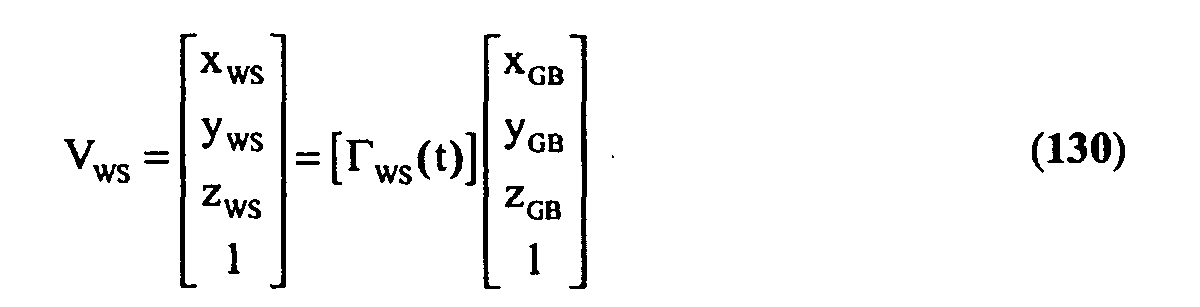
- Thus, the transformation matrices for translation of for the two relevant rotations may be written as
 and
and where X WS (t), Y WS (t) and Z WS (t) are the translation components of C WS versus C GB , Θ is the roll angle and Ψ(t) is the time-dependent yaw angle.
- The inverse transformation of vectors from the wheelset-based coordinates system C WS to the ground-based coordinates system C GB may be performed by the use of the formula
- The definition of Γ WS thus requires the assignment of a value to the parameter Θ and the definition of the time dependent functions X WS (t), Y WS (t), Z WS (t) and Ψ(t). The relatively small dimension of the axle together with the axle-mounted components and the short longitudinal distance between them and the sensors whose measurements are used to compute the Γ WS time-dependent components allow to use very simple expressions of X WS (t), Y WS (t), Z WS (t) and Ψ(t) for the short time interval corresponding to the application of the Γ WS function for a certain wheelset. Particularly, a linear dependency could be sufficient for expressing X WS (t) while a parabolic expression could be sufficient to express Y WS (t), Z WS (t) and Ψ(t). The discussion below about the computation of the Γ WS function will however show that the quality and the quantity of the measurements which may be used to define X WS (t), Y WS (t), Z WS (t) and Ψ(t) may be such to imply that all or some of these time dependent quantities can be assumed as constant or linearly expressed.
- An alternate particular position of the origin of the C WS axes is the centre of the axle, i.e. the point on the symmetry axis of the axle that lies at equal distance from the wheel flanges. However, regardless of the choice of position for the origin of the C WS axes, it is convenient to consider the axle as a cylindrically symmetric item, with the exception of the bearing that generally lacks such symmetry and does not rotate. Consequently, the rotation of the axle and of the components fixed to it may be generally neglected, with some possible exceptions related, for instance, to the web of corrugated wheels or to the slits or the holes in some visible components of brake disks. In other words, the C WS coordinates system is integral with the axis of an axle and with the axle-relates components, such as a bearing box, that do not roll over the rails. Consistently with these considerations, the pitch term was neglected above in the expression 131.
- The computation of the parameters that define the relevant angular rotations and the linear displacement components of Γ WS may be accomplished by the minimisation of the quantity δ2, which may be expressed by the chi-squared-like formulawhere the U values δ u and their corresponding uncertainties σ u correspond to the matching of wheelset items positions over time with one or more relevant measurements.
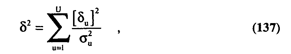
- Assuming that wheels sensors are accurate enough, the times t j',k' referring to the passing event of the centre of an individual wheel j' on the individual sensor k' may be directly very useful in determining the Ψ and the Y WS components of Γ WS by the expression
- The two δ u termsand
 where the integration limits are set in correspondence to a measurement interval for the wheelset taking velocity into account, may be used to define the first and second derivative vs. time in accordance with the LDF function defining Z(t), leaving other terms such as 138 to defme the offset. These conditions may be of course defined or written in different ways and, depending on the interpolation expressions for Z WS (t) and for Z(t), developed into closed form equations. As a matter of fact an offset exists in general between the LDF or Z(t) for a vehicle and Z WS (t) but such offset is irrelevant in the expressions 139 and 140 where the first and the second derivatives of Z(t) and Z WS (t) versus time are used.
- If one or more fast laser distance meters are installed in a similar way to Fig.8, their data may be very valuable to determine the Γ WS . In particular the use of the method discussed above for a F1 feature (about the computation of Ω) with one or more fast and accurate laser distance meters will be very effective for determining Y WS (t) and contributing to the definition of Ψ(t), depending on the origin chosen for C WS . The same data would also be very effective to define Z WS (t) and Ψ(t) by detecting the trailing and leading edges of the wheels. The relevant expressions and computational algorithms for the correspondent δ u terms may be readily defined, considering the examples given above for the definitions of the alternatives for the ζ r terms.
- X WS (t) may be defmed by the measurement of the wheel radius (e.g. ref. the discussion of Fig.8 above), taking into account the actual position of the railheads, as discussed below concerning the System calibration. Furhermore, if single VIS or NIR imagers (or pairs of imagers with the viewing planes preferably lying in the same almost vertical plane) are installed at low height so that high quality images (or high quality stereo images) of the wheels, and particularly of their lower parts, are obtained, the circular features corresponding to the flange rim or to the circular edges at the outer wheel face may be recognised and located in space versus time. The localisation of the circular features may be particularly reliable because the vehicle database information about the (unworn) wheel together with the wheel sensors timing allow a strong restriction of the allowable ranges of position, orientation and curvature. The relevant computational procedure may consist in a first step of selecting series of pixels which match admissible arches in an image and in a second step where a correct matching with the actual wheel circular features is searched. The corresponding expressions for the δ u terms would use the matching between fixed or variable diameter circles (depending on wear relevance) and the imaging vectors for the selected pixels at the relevant imaging times. Such a processing method of the linear images may consent to define X WS (t) Y WS (t), Z WS (t), Θ, Ψ(t) and the rolling radius with a very good accuracy.
- It is also possible to recognise the bearing box by pattern recognition and matching its position, retrieving the image of the bearing box and it position relative to the axle centre from the vehicles database. In this case the relevant images for pattern matching should however be acquired with a very similar imaging geometry by the same of by equivalent linear imagers. Such a need for a high similarity in the viewing geometry may however be decreased if the pattern matching software component uses relatively sophisticated or customised algorithms.
- The values of σ u for the expression 138 or for the δ u term related to a fast laser distance meter or for the image based method described here above would be principally defined as a function of the sensors measurements accuracies while for δ u expressions like 139 and 140 an empirical choice may be preferable.
- In general, the computation of Γ WS is obtained by an iterative procedure for multi-parameters search of its minimum value. In case the linear images method described above is used, the first convergence iterations should take into account only the simplest and more robust δ u terms, such as 138, 139 and 140.
- A second step in the diagnostic procedure for axle-mounted items concerns the determination of representative temperature values for the relevant items or for parts of them. This is achieved by associating the BWBTIS measurements to axles-related items by knowing their surfaces positions in the C WS coordinates system from the vehicles database and applying the Γ WS coordinates transformation on the relevant measurement vectors. The actual method must also take into account the visibility of items, the vectors matching uncertainties and the finite dimensions of the measurement beams.
- The axles-related items may be described in the vehicles database as a set of small polygonal flat surfaces (typically triangles or quadrilaterals like for "3D mosaics") or by a combination of polygonal surfaces, sets of cylindrical surfaces, cone frustums surfaces, circular surfaces, etc. Each of such surface items is associated to a mechanical item and is associated to a set of parameters, which depend on its geometry and define its shape, size, position and orientation in the C WS coordinates system. In general, it is advisable that the whole "visible surface" of a mounted axle with its related components is put in correspondence with such surface elements. Considering that the same axles and wheelsets or even the same entire bogies are mounted on different rail vehicle models, it may be convenient to store their surface description once and refer to it in the vehicles database, specifying the position of their C WS coordinates systems in the C VB coordinates system of a vehicle model. In general, the level of detail that should be used in such coding of the axle-related surface depends on the criticality of certain geometrical details in terms of the related performance and false alarms rate of the diagnostic method or methods.
- The specific parameters (i.e. for the particular axle under consideration) to be used in the diagnostic procedure based on the procedure for BWBTIS measurements are generally different according to the type of BWBTIS equipment used in the System and depend on the actual processing method. In any case they are stored in the vehicles database in association to a type of axle or a type of bogie or to a particular vehicle model, depending on the software implementation design and on the independence of such axle-related diagnostic parameters from the actual bogie or vehicle model.
- The term "HTDS" for "Homogeneous Thermal Diagnostics Surface" is used hereby to define a surface that may be considered as thermally homogeneous for diagnostic purposes. Some examples of HTDS are a vertical surface of bearing box parallel to the train movement direction, a low portion of a cylindrical surface of a bearing box, an outer portion of the surface of a brake disc and a bare cylindrical portion of an axle. Another particular example of HTDS is the lower part of the flat outer face surface of a wheel tyre, which may have a significantly higher temperature than the overall outer flat surface of the wheel tyre for a brake-blocked wheel. An HTDS can be coded in the vehicle database by one or more geometrical surface elements. A convenient way to code an HTDS is associating it to a sub-set of the geometrical surface elements mentioned above for coding the axle-related surface. Thus, the whole observable surface of a certain axle-related item may be composed of a series of coded surface elements with only one or a few of them constituting a certain HTDS for diagnostic purposes. A certain geometrical surface element may correspond to more that one HTDS, like in the case of different portions or of the whole of a wheel tyre plane outer surface.
- A first method, hereby referenced to as "TAM1" for Temperature Assignment Method 1" to assign a representative temperature to an HTDS applies to the case for which one or more BWBTIS measurements may be securely referred to an HTDS. For such TAM1 measurements the instrumental reading should be practically unaffected by the temperature of any surface close or contiguous with the relevant HTDS, in the view by the relevant BWBTIS (without considering the variation of the HTDS actual temperature due to heat exchange with such other surfaces). In practice, the uncertainty in the position of the HTDS vs. the measurement beam vector and the measurement beam footprint on the HTDS must together be such that the BWBTIS views only portions of the HTDS, i.e. no significant portions of any other surface. Fig.19 a is a conceptual illustration of the conditions that make TAM1 applicable. The triangle 700 exemplifies an HTDS while the two surfaces 701 and 702 are namely located behind and in front of surface 700. The measurement beam cross sections from 703 to 708 ideally refer to a single passive infrared sensor and the whole image of Fig.19 a is defined as a view from an infinite distance along the optical axis of the measurement beam. The measurement spot 703 is visibly larger than the others because of the divergence of the measurement beam. The larger ellipses, such as 709 and 710, indicate the area to which the corresponding measurement spots could be referred to, taking into account the spot position uncertainty vs. the observed surface. In general the "geometrical correspondence uncertainty" is different in different directions, according to the accuracy in the measurements and in the Γ WS transformation. The two axes of the measurement spot ellipses and of the larger ellipses resulting from position uncertainty do not generally coincide and in the drawing they are purely casual. In the example of Fig.19 a, only the 705 and 706 measurement spots strictly satisfy the eligibility requirements for the application of TAM1 to the HTDS 700. The temperature assigned to the HTDS by TAM1 is just the average of the single relevant temperature readings. Obviously, the applicability of TAM1 is favoured by a more accurate Γ WS transformation, more accurate HTDS definitions, larger HTDS dimensions, measurement view angles closer to normal vs. the observed surface, higher data acquisition rates, higher sensors bandwidth, narrower measurement beams, lower vehicle velocity, closer angular spacing between the beams for two adjacent pixels (if applicable) and a faster mechanical scanning rate (if applicable).
- Fig.19 b, represents the same case of Fig.19 a but with a much wider measurement positioning uncertainty along the direction of the series of measurement spots 723 to 728. In this case, the envelopes such as 729 and 730 to assign a measurement to a surface element are relatively so large that no measurement spot can be securely considered as purely representative of the HTDS 720, since they could partially overlap to the other surfaces 721 and 722. Therefore, TAM1 is not applicable in the case of Fig.19 b. A special characteristic of the measurement spots and of their corresponding position uncertainties in Fig.19 b is that, at least two of the measurement spots must be fully overlapped with HTDS 720. If such special situation applies, a second method, hereby referenced to as "TAM2" may be applied to define a representative temperature to an HTDS. TAM2 makes use of the fact that the maximum difference between the temperature readings of those points, which fully overlap to the HDTS 720, may be estimated by the NETD (Noise Equivalent Temperature Difference) of the measurement instrument and by the further measurement spread contributions deriving from the largest expected variability over the HDTS of surface temperature and of surface emissivity. Such overall maximum spread may alternatively result from the statistical processing of actual measurements. TAM2 may be satisfactorily applied if the temperature readings for the "contiguously viewed" surfaces, such as 721 and 722 are sufficiently different from the ones for the relevant HTDS. In fact, if such conditions apply, a search can be made of a series of measurements within the above-mentioned maximum spread and "surrounded" by statistically different values. The representative temperature for the relevant HTDS according to TAM2 is thus defined as the average of the measurements that are found within the applicable variance for eligibility.
- Fig.20 a exemplifies another possible measurements situation in which the width of the viewed portion of an HTDS is comparable or smaller than the measurement spot width. The surface 741 is an HTDS positioned between two other surface elements 740 and 742. The 14 measurement spots such as 743 are centred over the line 744 and largely overlap with a few other spots being close to them. No indication is shown in this drawing of the areas corresponding to positioning uncertainty. In this particular conceptual example, the sampling rate is such that the measurement spots largely overlap. An example of a practical situation similar to this case may be the observation of a part of a brake disc, like in Fig.17 a and Fig.17 b, from a sensor positioned outside the space between the rails and with the effect of measurement beam divergence causing the spots to overlap at the distance of the HTDS from the sensor. Fig.20 b refers to temperature measurements corresponding to Fig.20 a. The axis 745 indicates the actual or measured temperatures while axis 746 may correspond to a spatial linear coordinate over line 744. The actual temperature graph 747 assumes that each of the three surfaces 740, 741 and 742 have a homogeneous temperature. Each or the measurement bars such as 749, 752, 750, 751 and 748 corresponds to the reading for one of the measurement spots of Fig.20 a. The vertical length of the measurement bars corresponds to the NETD of the temperature reading instrument and the clearly visible average offset of the initial and of the last measurements in the series, such as 748 and 749, vs. the curve 747 results from the temperature measurement error related to different emissivity values. A third method, hereby referenced to as "TAM3" may be applied in certain cases like the one of Fig.19 a to assign a representative temperature to an HTDS, based on the computation of a fitting curve such as 749 in Fig.20 b. This type of curve fitting problem is known from other application domains and is discussed in several open literature articles and books in the field of experimental physics. The actual shape of the curve depends on the beam profile, approaching a smoothed square peak when the spot size becomes small versus the width of the HTDS. An accurate definition of the Γ WS transformation function together with an accurate coding of the HTDS surface makes TAM3 particularly robust. Furthermore, is the measuring beam profile vs. distance is also accurately known, the curve fitting process may yield an approximate estimation of the HTDS temperature even when the ratio between the HTDS width and the spot width is smaller than in the case of Fig. 19 a and, correspondingly, a higher difference exists between the maximum measured value, such as 750 and the actual HTDS temperature. If the spots positions are known with a large uncertainty (e.g. along 744 in the case of Fig.20 a), the TAM3 method may be applied, leaving the necessary spatial offset flexibility to the fitting function, providing that the surface surrounding the peak are known to be at a significantly different temperature. The homogeneity of the temperature of the surrounding surface is another factor making the TAM3 successfully applicable in this last particular situation.
- TAM1, TAM2 and TAM3 are discussed above, with references to Fig.19 a, Fig.19 b, Fig.20 a and Fig.20 b, for series of measurement spots aligned along a row but they should be considered as generalised to sets of measurements whose beams are scattered in two angular or displacement dimensions, depending on the types of sensing instruments and on the projection used to map the geometrical data.
- A fourth particular method, hereby referenced to as "TAM4" may be applied in certain cases to assign a representative temperature to one or more HTDS for a data set encompassing a few surface elements. An example for which this method may be particularly appealing is the case of a bearing box together with its corresponding solid wheel web, with temperature measurement data being measured from the track side by a device of the second or the third group of BWBTIS mentioned above. In this case, four HDTS could be defined for a representative portion of the bearing box surface, for two portions of the web on the leading and the trailing sides of the axle and for a portion of the web just below the bearing. A temperature function of the three spatial dimensions in the C WS coordinates space may be defmed over the relevant surface (bearing box and wheel web), with the sufficient flexibility to describe the "transition areas" between the different HTDS but with a sufficient stiffness to allow a reliable convergence of an algorithm to match it with the BWBTIS data by limited adjustments of the Γ WS transformation parameters. A principal advantage or this method is its possibility of achieving a good performance in the presence of a relatively poor accuracy of the Γ WS function, e.g. with reference to the X WS component. The principle of this method may be applied as well to BWBTIS data series in a row, such as the ones produced by the first type of BWBTIS mentioned above.
- All the four temperature assignment methods outlined here above require that series of BWBTIS data are mapped, using the Γ WS transformation over the surface elements defined in the vehicles database. Like for the methods discussed above for the detection of gauge-related defects, the computations for matching measurement beams and surface elements may be performed in the C WS or in the C GB coordinates spaces, namely using the Γ WS transformation on the measurement beams data or using the inverse transformation to convert the surface elements positions and orientations to the ground-based coordinates. The uncertainties in the relative positions and/or orientations of measurement beams and surface elements may be estimated using standard methods, depending on which data are used to defme the Γ WS parameters, on their accuracy and on the processing methods used in the Γ WS parameters definition. Different computationally efficient algorithms may be used to define the cross-sections of a measurement beam with one or more surface elements, including some of those that have been published in the open literature concerning the visualisation of three-dimensional vectorial drawings or optical ray tracing. The conversion of all measurement beams geometrical data from the C WS to the C GB coordinates space or vice versa is unnecessary and it would imply a waste of computing resources. Thus, it is advisable that coordinates conversion is applied only to the data for the measurements that are candidate for a possible matching with the relevant surface elements. The Γ WS function may be used to accomplish this by defining time intervals, and, if applicable, pixels or scanning angles ranges, taking an uncertainty margin into consideration (some limiting surfaces enclosing the axles-based components and the BWBTIS geometrical data are suitable to perform the computation). Several algorithmic solutions may be implemented by the technicians to reduce the computational burdening associated to the processing of the BWBTIS data. As an example, if several BWBTIS data can be mapped for a certain HTDS, some sub-series of them may be assigned without computing the beams intersections with the HTDS surface is they are securely geometrically comprised between two or more measurements assigned to the HTDS.
- A fifth particular method, hereby referenced to as "TAM5" to assign a representative temperature to one or more HTDS for a mono-dimensional or bi-dimensional data set when the possible variations in the view of the relevant surface elements is relatively low (e.g. there is no hiding or important shrinking of an element due to a change in bogie yaw or for different wheel wear extents). TAM5 is based on the processing of a "pseudo image" of the axle-mounted components, i.e. a mono-dimensional or bi-dimensional array of temperature measurements characterised by two spatial variables, e.g. the viewing pitch angle for the pixels of an infrared sensors array and the longitudinal displacement. The coordinates of the pseudo-image array components are slightly shifted or deformed in order to maximise a matching based on the homogeneity of temperature for certain regions corresponding to one or more HTDS. An accurate Γ WS may not be required in the case of TAM5. This method may be seen as a form of pattern matching using a pattern with some flexibility or allowing some deformation of the data set to be matched to a rigid pattern. TAM5 differs from the former TAM1 to TAM4 methods because three-dimensional coordinates are not explicitly used but it has in common with them the use of specific information from the vehicles database.
- Other temperature assignment methods may be defined by engineers skilled in the relevant arts, making use of geometrical computations and signal processing methods with the goal of maximising the accuracy of temperature estimation relating to the HTDS elements defined in the vehicles database.
- The methods to be used for processing the axle-related passive infrared sensing data are specified in the vehicle database together with all the necessary parameters and information for their application.
- The Applicant specifies that, in case a commercial BWBTIS device or a modified version of it is integrated in the system and such device produces a satisfactory estimation of the temperature of an HTDS (absolute or relative to ambient) the value produced by such instrument can be used in the next step of the procedure for axle-related items thermal diagnostics. The last statement holds also in the case such integration consists in the use of a "scanner" and in running the relevant data processing software on a separate hardware, which may be part of the computing hardware of the System. In these cases the System will be anyway advantageous vs. the prior art even though no use is explicitly made of the Γ WS transformation. The specific information from the vehicle database will in fact allow the achievement of a better balance of defect detection performance and false alarms rate.
- A third step is discussed here below in the thermal diagnostic procedure for axle-related items, corresponding to the recognition of hazardous conditions, based on one or more relevant BWBTIS measurements and on other applicable information and data.
- The condition to be met for generating an alarm or a warning message related to the measured temperature of a certain item may be written in the generic form
- The simplest degenerate form of 141 trivially corresponds to Π being the multiplication of T HTDS by 1 and Ξ being a constant value (this is equivalent to checking if the T HTDS is equal or greater than a certain alarm threshold temperature value). Such a degenerate form is however known to be poorly applicable to the hazard detection problem discussed here and some important dependencies are indicated below for the functions Π and Ξ in order to enhance the hazard detection sensitivity while keeping the false alarm rate relatively low.
- The Π function may embody one or more dependencies to correct the value of T HTDS into a more accurate one, taking into consideration one or more issues that were not accounted for in the (hardware and software) process or processes used to obtain T HTDS from the elementary measurements made of BWBTIS electrical signals.
- Unless dual-wavelength (ratio) or multi-wavelength thermometry is employed (by the use of special BWBTIS instruments), an important example of a Π function correction is related to the HTDS emissivity. The emissivity correction requires the definition of a function that depends on the spectral sensitivity of the actual measurement instrument and on the nature of the observed surface. The correction function is generally non-linear. In the case of interest, the HTDS emissivity may be quite different for different items (from high-emissivity rusty items to low-emissivity shining surfaces of chrome-plated or polished metals and alloys) and may depend on the age and history of the observed item (oxidation, paint peeling, soiling, etc.). An advisable manner to perform the emissivity-related correction is to store and retrieve the specific function parameters (e.g. using a polynomial form) in the vehicles database, for a particular HTDS. Such specific correction definition may be limited to those items for which the correction is more important. The actual correction parameters may be defined on the basis of specific statistics or by defining a set of "reference corrections" to be used for classes of items (e.g. aluminium alloys, stainless steel, painted iron subject to peeling and rusting, etc.). The vehicles database will be the source of the information specifying which correction class should be applied for the relevant HTDS of a certain item. Standard deviations may also be defined for the emissivity correction parameters for specific items or classes of items (or for the corrected temperature), to be taken into account, as appropriate, in the Π function.
- A second example of a Π function correction is the compensation of the ambient temperature radiation when the HTDS has a low emissivity (and thus a high reflectivity) and the temperature of the surrounding environment is relatively high (the correction may be based on the measurement of ambient temperature or on the readings of certain BWBTIS when they are measuring the background thermal radiation).
- A third example is the compensation of the ambient temperature effect on the reading of the BWBTIS instrument when the compensation of the changes in the temperature of parts of the BWBTIS instrument is insufficient. This correction can be made by measurements carried out by temperature sensors installed within the relevant instruments and/or by ambient temperature measurement of by external calibration sources (with fixed or controlled temperature and position).
- A fourth example is the compensation of measurement drift by the use of external calibration sources (with fixed or controlled temperature and position).
- The Ξ function may be considered as a specific defect detection threshold value to which the Π value is compared, possibly within a tolerance expressed by the term γ.
- It is well known to those skilled in the art that, for the mechanical items of principal interest in this discussion, i.e. axle bearings, under certain operating conditions (e.g. the loading of a wagon) and following a certain operation history (e.g. having travelled over the last tens of minutes at a certain speed), the variance of the threshold temperature corresponding to a certain failure or incipient failure condition is dramatically reduced if ambient temperature is used as the thermometric zero. In other terms, the excess temperature of a bearing box over ambient temperature caused by (normal or hazardous) friction has a small dependence on ambient temperature itself. The principal physical reason for this is that the dominant heat dissipation mechanism (convection) depends almost linearly on the temperature difference between the heated part and ambient air. Additionally, the variation of heat generation by friction is not highly dependent on temperature. Thus, a simple definition of the Ξ function may be the sum of ambient temperature to a certain threshold temperature value that may be obtained from the vehicles database.
- If the wheelset load is known to the System, a further additive term being a function of vehicle load may be added to the Ξ function defined here above. Particularly, but not exclusively, such term may be proportional to the vehicle load by a multiplicative coefficient and proportional to or a function of the bearing box temperature over ambient temperature, the relevant function parameters being specifically stored in the vehicles database.
- Another term could be defmed if the System could obtain (from the train or from a railway information technology system) the information on the recent travelling history (distance run and velocity profile).
- A particular term could be embodied in the Ξ function to account for the extra heating of the HTDS for a bearing box when the corresponding wheel is at an elevated temperature as a result of braking. This term would depend from the actual construction of the axle assembly and therefore could be specific and stored in the vehicles database.
- It is also well known to those skilled in the art that an effective way to define the alarm threshold temperature values for axle-related components [011] is computing them as the average of the temperatures for other identical items on the same vehicle or even on the whole train, plus an allowance that may be defined as a multiple of the standard deviation of such temperatures. The rationale for this is that all such identical items underwent the same history in terms of travelled distance, velocity vs. time, ambient temperature and (for brakes and wheels) braking activity. If the items are exposed at the side of the vehicles (e.g. in the case of bearing boxes), the averaging may be made more relevant by separately performing it for the two sides of the train so that the exposure conditions to solar radiation and to wind are also taken into account. The temperature of items exceeding a certain temperature over ambient or exceeding a multiple of the standard deviation over the average temperature of the identical items should be excluded from averaging. The identification of the vehicles in the Method allows using this averaging approach more effectively than in prior art because the System may securely select the identical items for the averaging computation. Additionally, the System may refme the alarm generation criteria by the use of specific parameters applicable to a certain type of mounted axle, retrieving them from the vehicles database.
- Thus, indicating by T HTDS,m the T HTDS temperature value for a member m of a group of identical items, the expressionmay be used within the System software as a statistical alarm condition for the overheating of bearings, brakes and wheels. The K' coefficient in 143 may be retrieved from the vehicles database (if it was specifically evaluated) of may be defined for classes of components. The exclusion of "abnormal items" from the N terms of the summatories in 143 may be done by different alternate algorithms, e.g. by excluding the items group members with the highest values of temperature T HTDS until the condition 143 does not apply for all the residual N items.

- In general, other and more sophisticated statistical tests may be used as a substitute to the simple statistics approach based on variance. Furthermore, different statistical tests may be used for the same specific item depending on the numerosity of the sample used for the analysis.
- In the particular case of axles bearings, the condition 143 may take into account some factors (e.g. wagon load on the axle and wheel heating) affecting the temperature of individual items or sub-sets of items by substituting T HTDS,j , T HTDS,k and T HTDS,i by T * / B,h as defined by an expression such as
- The Applicant specifies that the expression 144 is just a particular case of a generic mathematical expression
- Some types of BWBTIS may also provide measurements of the axles temperature and such measured values may be the subject of a dedicated alarm criterion or be used within the alarm conditions expressions for bearings and for brakes.
- The term γ in the above expressions may be neglected or it can be used to tune an alarm condition. Such role of γ may be however substituted by the tuning of some other, non necessarily additive, parameter within the alarm conditions discussed here above or in other conditions which may be defined for the same purpose.
- In general, more that one hazard detection criterion can be applied to a certain type of axle-related item and the vehicles database can indicate which criteria to apply for a certain vehicle or bogie type or mounted axle type, together with the parameters for the alarm expressions or the indication of the appropriate class of axles for which such parameters have been defined.
- In case a complete high performance commercial device is used to perform the detection of axle-related thermal defects, the System may provide to the processing unit of such device a set of vehicle-specific information, which may be used to apply its own diagnostic criteria in a more specific and effective manner. Such an arrangement would be a particular implementation case of what discussed above.
- The value of ambient temperature to be used in the computations to diagnose the above mentioned axle-related hazards may be obtained in different standard means and particularly by an appropriate temperature probe or even a local meteorological station, whose other data may useful for other purposes.
- A considerable effort was devoted in the past to the problem of distinguishing sleeve bearings from roller bearings (in order to apply different alarm criteria) or to define alarm criteria that were applicable to a population including both types of devices. In this respect, the Applicant clarifies that such issue has not been addressed in detail in this text for the principal reasons that sleeve bearings have practically disappeared (e.g. in Europe they are banned from the vehicles subject to the RIV agreement). The Method and the System would however brilliantly solve the issue of the two types of bearings since the identification of the vehicles models implies the possible availability of any useful information about them, including the type (and even the model, geometry, position, etc.) of bearings, as discussed above.
- The text here below addresses the diagnostic functions that can be implemented in the System to detect overheating and fire on board of identified vehicles on the basis of passive thermal infrared measurements, of the computing of vehicle position over time and on the specific information that may be recorded in the vehicles database.
- The Method, in order to detect overheating and fire on board of identified vehicles, requires that series of appropriate measurements are taken of the thermal infrared radiation emitted by the vehicle body or by its load, in order to process them as explained further below. The requirements applicable to these measurements are very similar to the ones discussed above concerning the thermal diagnostics of axle-related components, even though, in the case of vehicle bodies and loads, the requirements for spatial resolution (in terms of positions of adjacent measurement spots on the observed surfaces), the thermometric resolution and accuracy, the measurement bandwidth and the sampling rate may be less stringent. Also in this case the Applicant does not specify stiff requirements figures for the relevant passive infrared sensors but it will result clear from the discussion of the data processing methods below how the characteristics and the installation parameters of such sensors affect the System performance concerning the detection of overheating and fire on board of identified vehicles.
- Fig.21 a and Fig.21 b show a possible positioning for a linear infrared passive imager 760 or 768 performing its measurements for one side of a vehicle and a portion of its surface facing up. Fig.21 b is not exactly a different view of the installation corresponding to Fig.21 a because the positions and orientations of the shown measurement instruments are not the same (angle 772 is null in Fig. 21 a). Only one infrared imager is shown in both Fig.21 a and Fig.21 b but, of course, another correspondent imager would be installed, symmetrically, for the other side of the vehicles. Additionally, further imagers could be installed in different positions and with different orientations.
- If linear infrared imagers are used, the spacing 767 between two measurement spots corresponding to adjacent pixels (normal to one of the two relevant measurement beams 763 and 764) obviously depends on the distance between the observed surface and the imager. If, for instance, the thermoelectric linear imager "Model IR 1000" [068] described above is used with a field of view (angle 765 between the extreme measurement beams 761 and 762) of about 65 deg, the approximate value of length 767 for the central pixels of the array ranges from about 13 mm at 1 metre distance to about 65 mm at 5 metres distance. Such two values of length 767 for a 256 pixels linear imagers at the same conditions are about 5 mm and 25 mm. Instead, the longitudinal spacing between two successive imaging beams, such as distance 775 between beams 773 and 774, only depends on the array scan rate and on vehicle speed (for instance it has an approximate value of 33 mm at 120 km/h for a scan rate of 103 s-1). Naturally, the actual incidence angles between the measurement beams and an observed surface will define the relevant distance between the centres of the measurement spots over the surface. As discussed for other instruments above, the decrease of angle 772 from 90 deg will affect the minimum value of angle 765 to accomplish the complete view of a range of positions over the vehicle. The depth of field of the optics is of course an issue and the optical resolution for two adjacent pixels should be appropriate for the distance range of interest, also taking into account the longitudinal spacing 775.
- IR passive scanners based on rotating mirrors (e.g. a modified version of the fast scanners [964]) are an alternative to linear imagers based on staring arrays and they may be considered for the System implementation.
- As discussed above for other instruments (e.g. for the VLDS) the choice of the number of units and their positions and orientations for a System implementation will result from balancing the eventual System performance with cost and maintenance considerations, taking into account the characteristics of the instruments (resolution, scan rate, etc.) and the installation constraints (with special reference to the case of installation for double or multiple rail tracks). The Applicant considers that the installation of two linear imagers at a position similar to the one indicated in Fig. 21 a may be sufficient to achieve valuable results from the data processing methods described below and that, particularly, both the types of linear infrared imagers discussed above and based on thermoelectric linear array or photoconductive PbSe arrays or fast linear infrared scanners may be successfully employed for the thermal infrared measurements of vehicles bodies and of their load. It is however possible to use other types of linear infrared imagers, or FPA infrared imagers or even series of instruments with one or a few thermal infrared sensors for each unit, providing that their measurement bandwidth, measurement rate, field of view and resolution are appropriate and that an accurate time value may be associated to each measurement.
- Fig.21 a and Fig.21 b also show the VLDS instrument 766 or 769 and a linear camera (VIS or NIR or colour) 770. The installation of the three sensing devices (IR linear imager, VLDS and linear camera) or two of them (IR linear imager and VLDS or IR linear imager and linear camera) with parallel view planes and with their measuring beams converging on a same line parallel to the rails is particularly advisable if, as discussed further below, the data produced from them are the subject of a common process. In fact, with such installation geometry, the relevant data for these different instruments may be easy matched (based on the Ω coordinates transformation, or just on the LDF, together with the instrument geometry calibration parameters) and with the principal advantage that the relative positions of foreground and background bodies on the vehicle are observed (at different times) from the same relative view point.
- The processing of the thermal radiation measurement data for the bodies of identified vehicles (including their loads) to detect overheating and fire hazards is based on the information contained in the vehicle database that, for the relevant model of vehicle, defines the actual diagnostic method to be applied and supplies the vehicle-specific data for applying the methods. Such methods are called hereby by the acronym "VBTHDM" (for Vehicle Body Thermal Hazards Diagnostic Method). Each VBTHDM makes use of one or more "TEPP" (the acronym used hereby for Thermal Emission data Pre-Processing algorithm), which deliver a few numerical values by processing the data from for a certain subset of thermal radiation measurements data corresponding to a "TESD" (the acronym used hereby for "Thermal Emission Spatial Domain").
- In general, a TESD is defined by a surface in the C VB coordinates system, as defined above, and corresponds, more or less accurately, to a physical surface that is a fixed part of the vehicle body or to a physical surface of an item on the vehicle without a predefined fixed position or to a certain "virtual envelope" defmed for the vehicle.
- A TESD1 is a geometrical surface that corresponds to a physical surface that is a permanent physical feature associated to a certain model of vehicle. TESD1 surfaces are defined in the vehicles database as rectangles or as more complex structures such as a mosaic of simple polygons such as triangles, flat surfaced with a polygonal contour or analytical geometrical surfaces such as portions of cylinders and cones. Some examples of correspondences between TESD1 and physical features of vehicles are a whole flat side wall of a closed freight wagon, a closed sliding door for that same type of wagon, a window of a passengers railcar, the flat upper surfaces of a closed wagon for transporting cereals in bulk, a cylindrical surface of the roof of a closed freight wagon or a louvred panel at the side of a locomotive.
- A TESD2 corresponds to a physical surface that has been detected on a certain vehicle by the System (based on measurements) and that does not correspond to an item that is a permanent component with a fixed position for vehicle model. TESD2 surfaces are generally defined as mosaics or by series of three-dimensional contours or profiles. Some principal examples of TESD2 are the sheets wrapping or covering loads on open wagons, the surface of heavy bulk materials in open wagons, solid bodies loaded on flat railcars and vehicles transported by piggyback wagons or cars on double deck wagons.
- A TESD3 surface is used to define a geometrical envelope that does not correspond to physical item but is useful to process thermal radiation data. A TESD3 is defined by surface elements as for TESD1. A noticeable example of TESD3 is a portion of the loading profile envelope for an open wagon. One or more TESD3 surfaces together may define a TESD3 volume, which is functionally equivalent to the corresponding set of TESD3 surfaces.
- The thermal radiation measurement data are associated to a TESD by the Ω coordinates transformation defined above or by the LDF, which may be viewed as a degenerate and limited case of the Ω function. Each thermal measurement corresponds to a measurement beam that may intersect (entirely or partially) one or more TESD surfaces. The computation of the intersections requires the use of said coordinated transformation function, of the geometrical and calibration parameters for the relevant thermal radiation measurement instrument and of the TESD data from the vehicles database. The uncertainty in the determination of such intersections should be taken into account, as discussed above for the processing of BWBTIS data.
- A measurement beam may be put in correspondence with one or more TESD, depending on its full or partial intersection with such surfaces and on the "transparency" of the relevant TESD surfaces. The "TESD transparency" may be defined as a number between 0 and 1 that expresses the average fraction of infrared radiation that is assumed can traverse such surface. The corresponding "opacity" of a TESD surface is the complement of transparency to unity. A minimum and maximum transparency value may be defined for each TESD. Transparency may also be defined as a function of the beam incidence direction at the TESD. TESD3 surface are completely transparent while TESD1 surfaces are by default totally opaque unless transparency has been specified (e.g. in the case of a louvred plate or a metallic net). The transparency of TESD2 surfaces could be determined, if required, by an algorithm that may be defined taking into account the characteristics of the relevant three-dimensional measurement system and of the thermal measurement system (with special reference to the spacing between adjacent measurement beams and to the beams cross section, for both types of instruments).
- For each measurement beam, a set of "assignment coefficients" (hereby also called "BAC" for Beam Assignment Coefficient") may be computed by determining the intersection of a beam with the series of TESD surfaces that such beam encounters starting from the measurement instrument and going towards the background. An "intersection fraction" (hereby also called "BIF" for Beam Intersection Fraction") may be defined (with more or less complex algorithms) to quantify the relative cross section of a measurement beam with a surface, with a unity value when the intersection is complete and a proportionally lower value for a partial intersection, possibly taking into account the actual beam profile (and considering the relative uncertainty in beam direction and relative positioning). A "beam relative integrity" equal to 1 is assigned at the beam before any TESD surface intersection. The intersection with a surface subtracts from the beam relative integrity a fraction corresponding to the relevant BIF multiplied by the opacity of that surface. The BAC for a TESD surface is given by BIF multiplied by the beam relative integrity "reaching" that surface. If transparency is defined by a range (not by a single value), different criteria may be used to assign one or more BAC values. BAC values may be generally considered as "fuzzy" variables, except for the case of unity value, which is a very common one and corresponds to a full assignment of a TESD surface to a measurement beam.
- The Applicant clarifies that this formalism using the BAC values to assign the correspondences between measurement beams and surfaces is convenient way to formalise the issue of measurement beams intersection with TESD but it may be substituted by other formalisms with a similar, higher or lower level of complexity. The process of assigning a measurement beam to one or more TESD surfaces may be limited to establishing total or partial correspondences (with or without the definition of BAC values) or can also include the computation of the coordinates for the intersection centres. The beam intersection profile at the surface and the relevant variance values may also be computed if required for a TEPP.
- The temperature values that were obtained from the thermal infrared radiation measurements may be directly used within the TEPP computations or, in the case of TESD1 surfaces, may be subject to a correction as discussed above for the THTDS measures from BWBTIS instruments, to take emissivity and other factors into account (based in on the relevant information associated to TESD1 surfaces in the vehicles database).
- TEPP1 is a simple way to process thermal radiation measurements for an opaque TESD1 surface and consists in computing the average value (and possibly the standard deviation or other statistical momenta) for the measurement beams with BAC equal to 1, i.e. with no overlap of the beams with any other non-transparent surface. TEPP1 is therefore ideally applicable to TESD1 surfaces with a sufficient area (relatively to the spacing and to the beam profile of thermal infrared measurements) and for which a substantial homogeneity of temperatures is expected. TEPP1 thus corresponds to the TAM1 method defined above for the HTDS of axle-related items.
- TEPP2 applies to relatively small TESD1 surfaces where no relevant measurement beam has a BAC value of 1. The methods defined above for TAM2 can be applied in this case to compute a representative temperature value and, possibly, a corresponding uncertainty estimation.
- TEPP3 corresponds to a partially transparent TESD1 surface in front of another TESD1 surface and applies to measurement beams with BIF equal to 1 for both such surfaces. The statistical distribution of the measured temperatures is computed and the average is made of two measurement sets namely including the N L lowest and the N H highest values. N L and N H are specified for the relevant VBTHDM or computed by an algorithm that takes the total sample size into account. TEPP3 is indicated for "semi-transparent" surfaces with slits or holes and solid parts having a minimum width larger than the thermal measurement maximum beam spot diameter at the foreground surface (it is therefore expected that some beams are totally or almost totally intersecting one only of the two TESD1 surfaces).
- TEPP4 applies to the same case of TEPP3 but is based on the prediction of the foreground and of the background average temperatures, assuming a certain beam profile at the foreground TESD1 surface and a certain structure of the same surface (typically described as alternated slits and stripes or holes in a panel). TEPP4 is indicated for "semi-transparent" surfaces with slits or holes and solid parts having a minimum width smaller than the thermal measurement maximum beam spot elliptic diameter at the foreground surface.
- TEPP5 applies to relatively large TESD1 or TESD2 opaque flat surfaces where one or more warmer area(s) may appear while some other areas keep at a homogeneous lower temperature. Cylindrical surfaces may be "converted" to equivalent plane surfaces. The measurement spots centres are first mapped in two dimensions over the flat or flattened TESD surface. A discrete map or a "pseudo-image" is thus defined and compact clusters of warmer spot(s) and the cool spot(s) are identified and characterised by suitable algorithms. One possible such algorithm is based on defining a set of binarisation thresholds (e.g. based on a global histogram of temperatures) followed by the generation of binary images to which "blob analysis" is applied. Other alternate algorithms can be used such as the fitting by "bi-Gaussian" functions (temperature vs. the orthogonal coordinates of the TESD surface with the axis of the elliptical contour lines rotated by an angle to be fitted) after searching for local maxima and minima (to define the coordinate of the bi-Gaussian functions centres) over a map obtained by applying a two-dimensional smoothing to the thermal data map. TEPP5 requires the definition of a few parameters to constrain the search for the warm and for the cool spots (e.g. minimal cluster size, maximum corresponding temperature range by absolute values over ambient temperature or relative to the temperature values range, etc.). The output of TEPP5 consists of a series of representative temperatures (maximum and/or average) for warm and cool spots, possibly associated to their coordinates, elliptic diameters and one or more measurements of statistical spread.
- TEPP6 is equivalent to TEPP5 but limited to the higher temperature portions of the relevant TESD.
- TEPP7 is equivalent to TEPP6 but it applies to TESD2 surfaces and the temperature values taken into considerations are the ones beyond a certain percentile of the relevant histogram.
- TEPP8 is defined for the same data mapping of TEPP5 but a histogram is computed of temperature values after a two-dimensional smoothing operation. The histogram is preferably normalised by the surface areas that may be referred to each single measurement on the basis of its average distance to the adjacent measurement spots centres.
- TEPP9 is defined for TESD1 opaque surfaces and has the goal of recognising the presence of warmer temperatures in correspondence with one or more lines on the surface. TEPP9 may be based on different formulas and computation procedures (computing of covariance, pattern matching, etc.) and the lines may be defined in the vehicles database by their position or just by constraining their minimum length and relative orientation.
- VBTHDM1 is a relatively simple method based on average temperature values from TEPP1, or on the spot temperatures from TEPP2 or TEPP6 or TEPP7 or TEPP9 or on the foreground and background temperatures from TEPP3 or from TEPP4. Alarms are generated when a high temperature from the processing by the relevant TEPP (under the constraints and the processing parameters defmed for such TEPP) exceeds ambient temperature by a certain threshold, which is defined for the relevant TESD surfaces of a vehicle model. VBTHDM1 has the advantage of being usable for a single TESD without requiring the availability of other TESD to be used as a reference. It has however the limitation that temperature variability due to solar irradiation or to heating sources in the vehicle cannot be taken into account, with a resulting general lower sensitivity within the constraint of a low false alarms rate.
- VBTHDM2 may be based on average temperature values from TEPP1, higher or lower temperatures from TEPP2 or TEPP5 or TEPP6 or TEPP7 or TEPP9 or on the foreground and background temperatures from TEPP3 or TEPP4. Alarms are generated when at least one higher temperature from the processing by the relevant TEPP (under the constraints and the processing parameters defined for such TEPP) exceeds by a certain threshold value a reference temperature value computed by the same TEPP or a different TEPP and applied to the same or to different TESD surfaces. The values from more than one TESD may be used to define the low temperature reference by averaging them, possibly excluding the values which fall outside a certain variance multiple. VBTHDM2 may allow an improvement in sensitivity versus VBTHDM1, with reference to the effect of solar radiation when the reference and the alarm TESD have the same orientation but such improvement is limited by the differences in thermal conduction and in the emissivity of the relevant surfaces.
- The applicable differential threshold values for VBHTDM1 and for VBHTDM2 can be specific predefined values or they may be defined by a function of the standard deviation from the relevant TEPP and possibly by a function of ambient temperature or of a lower temperature from a TEPP.
- VBTHDM3 is based on processing the histogram resulting from TEPP8. Diverse alarm criteria may be defined such as a fixed or computable threshold value for the difference between the average temperatures for certain fixed or computable percentiles intervals.
- VBTHDM4 is based on the statistical significance of the difference between a higher temperature derived from a TEPP (particularly from TEPP1 or TEPP2 or TEPP3 or TEPP4 or TEPP5 or TEPP6 or TEPP7 or TEPP9) and the average of a population of corresponding values for different TESD relative to the same vehicle or to a set of vehicles of the same construction model or part of a certain class of construction models. The statistical significance may be defined according to a standard statistical significance criterion. A condition similar to the one of expression 143 may be used.
- VBTHDM5 is based on the application of rules or mathematical expressions that define the alarm condition on the basis of more than one TEPP results. For instance one of two differential thresholds values is used for a pair of lower and higher temperature outputs from the same TEPP or from two different TEPP, depending on the range of the temperature output of a TEPP for a certain TESD.
- The application of a TEPP to a TESD2 surface requires that a suitable procedure is used to process the three-dimensional data defming the surface that normally corresponds to an unknown load on an open wagon and that appropriate geometrical constraints are specified by the parameters for the relevant VBTHDM to define the TESD2 within the overall surface defined by said three-dimensional measurements.
- TESD3 surfaces can be used when the three-dimensional measurement instruments installed at the SMI are not adequate to define the surface of a load on an open wagon. In this case VBTHDM1, VBTHDM2 and VBTHDM5 may be used, specifying that the high temperature values must be searched under constraints specified by a foreground TESD3 and by a background TESD1 or TESD3. In such a way, the measurements will refer to either a load (or a wagon sheet) or to the background, which will correspond to a wagon surface or to a wayside surface.
- The crude criterion of comparing an absolute temperature output from a TEPP (e.g. an average temperature from TEPP1 for a certain TESD) with a certain absolute temperature threshold value could be the basis for defining a VBTHDM, but the Applicant considers such a criterion of poor applicability, if compared to the VBTHDM alternatives described here above. In fact, for most relevant cases, the use of an absolute temperature threshold would imply a lower detection performance to avoid an unacceptable rate of false alarms.
- The Applicant clarifies that the above definitions of alternate types of TESD, TEPP and VBTHDM are not restrictive and exhaustive. Other TESD, TEPP and VBTHDM may be defined (by professionals skilled in the art) for the implementation of the System, still within the relevant claimed principles of the Method.
- Some considerations are made here below of the use of certain combinations of VBTHDM, TEPP and TESD for some principal types of rail vehicles, with the scope of exemplifying the application of the invention and to define certain specific advices for the application of some relevant parts of the Method.
- Fires originated inside closed wagons transporting miscellaneous freight and finally reaching a stage that may be highly hazardous may evolve with very variable rate of change and localization of heat release over time, depending on the ignition source, on the contents of the wagon, on the gaps between load items or between goods and their casing, on the three-dimensional loading pattern and on the reaction to fire, on thermal conductivity of the wagon walls and ceiling and on the ventilation of the loading volume. It is in particular possible that fire does not cause the collapse or the burnout or a very high temperature for any large part of the walls and of the ceiling for several tens of minutes after the ignition and for several minutes after the possible developing of a flashover condition inside the loading compartment. VBTHDM1 may be used in this case with various TEPP for specific TESD1 surfaces, such as in correspondence with ventilation outlets, or with TEPP6 for entire walls, panels and doors, with the principal limitation of setting the alarm threshold in such a way that worst-case solar heating does not trigger an alarm. VBTHDM2 with TEPP5 is a very effective solution that implies a rather simple and quick definition of the relevant TESD surfaces. In particular TEPP9 can be very useful for those wagons with insulating wall panels within metallic frames (forming a thermal bridge to the internal temperature) that are externally observable. Semi-trailers and containers are in general very similar to closed wagons for both fire dynamics and for the suitability of detection methods.
- Closed wagons for the transport of flammable solids in bulk (e.g. coal, wood chips, etc.) are subject to relatively low heat release rate flaming fires and more likely to smoldering fires which may develop very slowly and over long periods of time. A differential temperature criterion such as the one of VBTHDM2 or statistical criteria such as VBTHDM4 may result effective to locate a temperature increase on the sidewalls, while VBTHDM1 can be applied with TEPP1 or TEPP6 to the upper surfaces or to the sidewalls.
- Refrigerated wagons are a special case for the possibility that the refrigeration unit is a source of fire and because heat exchangers are normally at a higher temperature that "passive items" on the wagon. Therefore, the location of heat exchangers should be taken into account and some TESD may be defined in order to formulate a specific diagnosis of fire originated at the compressor unit. Some refrigerated wagons using polyurethane as an insulating material are particularly dangerous in case of fire in a tunnel because of the possible release of significant quantities of hydrogen cyanide from the polymer pyrolisis. The widespread preference for using low emissivity outer surfaces may however allow to increase the sensitivity of the detection method.
- Car transport wagons and HGV transport wagons are characterised by the variability of the load and a relatively high fire hazard. The optimal sensitivity adjustment for these wagons depends on the distance of the SMI installation from the nearest loading yard, because of the possible residual heat in tyres, engine, exhaust and brakes if the transported vehicle was stopped a short time before passing at the System installation.
- Passenger railcars fires are principally caused by arson and they may escalate to very hazardous stages depending on the fire resistance of the construction materials (with special reference to upholstered seats) and on baggage. Some general considerations made above for closed wagons apply for these railcars but with some special notes. Window frames behave in general as thermal bridges and may be suitable for applying TEPP9. Windows glasses, particularly if single, may heat up faster than sidewalls and may be used for defining TESD1 surfaces because their little transparency in the thermal infrared wavelength region (emissivity is close to 0.8 for most glasses wit a very low variance) allow to detect their abnormal heating. The presence of heating systems should be taken into account in order to achieve higher fire detection sensitivities, by excluding certain portions of the car body from the defined TESD surfaces. The fact that heating is applied when the external ambient temperature is low limits the sensitivity of VBTHDM1. The use of air conditioning may cause certain portion of the vehicle body to be cooler and this should be taken into account in defining the TESD and TEPP concerning the lower temperature reference. Sleeping cars are subject to a higher risk of non-arson-related fires because of the relatively high density of combustible materials, of their compartmentalization and for the ignition hazards from smoking in bed. They are however subject to the same detection methods consideration made for ordinary passengers cars.
- Locomotives are a very special case and are characterised by a relatively high fire risk, which is however very dependant on their model and generally on their traction type and generation. Diesel locomotives constitute a special hazard in tunnels due to the combination of fuel load and ignition hazards. The principal type of ignition hazard is not related to fuel tanks but mainly to the engine space, with special reference to the possible occurrence of a high-pressure diesel fuel spray from a leak. Diesel locomotives also have a number of warm and hot areas corresponding to engine and exhaust items and, even though the engine surface of diesel locomotives is enclosed in its compartment, it may be partially visible from louvred plates and be a possible cause of false alarms. Electrical locomotives are generally free of high temperature traction components but may exhibit high temperatures on their outer surface for the dissipation of heat, e.g. from the electrical braking system (particularly following a long and steep descending track stretch). Because of these particularities, the definition of VBTHTD, TEPP, TESD and of the relevant parameters should be, for each locomotive model, the subject of accurate and specific professional engineering considerations and a tuning of the detection process is highly advisable. The more complex TEPP computations and the use of VBTHDM5 may be necessary to achieve very high fire and overheating detection sensitivities within the low false alarms constraint.
- All types of vehicles subject to overheating and fire diagnosis according to the methods defined above require the definition of VBTHTD, TEPP, TESD and of the relevant parameters and the most advisable procedure for such task is a first such definition followed by one or more refinements. The availability of thermal maps from the System may be of great value in the first stage of method definition for a certain model of vehicle and the saving of the maps for all false and genuine alarms may be very useful to improve the detection process performance. The fine-tuning of detection methods by optimizing TEPP parameters may be conveniently performed by saving a large number of measurements data sets and refining the method off-line while the tuning of parameters such as differential thresholds can be adequately performed by the saving and the analysis of the TEPP outputs only.
- The Applicant annotates that, even though the subject is not discussed in detail in this text, it is possible to develop by those skilled in the art software algorithms and applications that make the methods refinement "quasi-automatic".
- In case some individual vehicles, e.g. a one or more locomotive items within a series, trigger an alarm while the other vehicles of the same construction model do not, it is possible to modify the hazard detection method to be applied for them, using the modified method when their serial number is recognised by the unique vehicle marking, which may be obtained for the large majority of vehicles within the marking code reading process in the vehicle identification procedure described above.
- The diagnostic methods described above may achieve a high performance or sensitivity within a low false alarm rate thanks to model-specific information and data and to the accuracy in associating measurements to certain known portions of a vehicle construction model. The text here below addresses some options that may be implemented in the System concerning diagnostic functions for the small fraction of vehicles whose model is not identified by the relevant procedures.
- Unless the decision is taken to omit the application of certain diagnostic functions or of all diagnostic functions for unidentified vehicles, different methods may be developed and applied to them, even though with a lower effectiveness if compared to the methods defined for vehicles whose model has been identified.
- Gauge profile diagnostics for the body of unidentified vehicles may be performed by a modified version of the methods described in section 5.9, on the basis of a coordinates transformation function Ω computed in a less accurate and robust way, by a modified version of the method discussed in section 5.8. The simplest way to compute the parameters of a less accurate Ω function is its limitation to the longitudinal displacement, which is defined by the LDF function. The definition of the other (angular and displacement) components may be based on the recognition of certain vehicle body features at different times along the SMI. The recognition of the same profile on both sides at certain appropriate heights may be particularly useful for defining the side displacement, the yaw term and the roll term. Principal components of buffers are a particular example of a feature that may be used for such purpose. An accurate measurement of the side displacement of the wheels at a plurality of longitudinal positions along the SMI may be useful by the computing of the lateral displacement versus time of the bogies castings or of the centres of single (non bogie mounted) axles. The vehicle (and load) allowable body profile to be used for one or more of the hazard detection conditions, such as 126, 128, 127 and 129, may be computed according to the methods of the UIC 505-1 standard [050] or to a similar method. The most relevant input to such profile computing corresponds to the positions of the bogies castings or of the centres of single (non bogie mounted) wheelsets, which are known from the LDF and WSD computation. Other input data, such as the vehicle flexibility coefficient, can be assumed, possibly as worst-case values.
- Gauge profile diagnostics for the lower parts of the vehicle may be performed for unidentified vehicles with a relatively low disadvantage versus a method based on vehicle model recognition, because roll and the issues concerning non-standard loading are less relevant.
- The diagnosis of overheating, failures and incipient failures in axle-related components for the unidentified vehicles cannot take advantage of the model-specific information and data. It is however possible to develop data processing algorithms (largely dependent on the type of installed BWBTIS) that perform the diagnosis in more or less sophisticate mean. The Γ WS function may be computed with a good accuracy at least for its longitudinal displacement and yaw components from wheel sensors data and used in the processing of BWBTIS measurements. The assignment of BWBTIS measurements to certain items such as bearings, wheels, brake discs and axles may benefit from the processing of VIS or NIR images. Measurements from fast and accurate laser distance meters can be useful to defme the wheel radius, which may be used to define the height of bearings over the rolling surface and the lateral displacement of a wheelset.
- The diagnosis of fire and overheating based on thermal radiation measurements for the bodies of unidentified vehicles can make use of the Ω function that, even though defined exclusively by the LDF function, is in general accurate enough for this purpose, and especially in the absence of model-specific information and data. Methods such as VBTHDM1 with TEPP1 or TEPP5 or TEPP6 may be employed, even though the thresholds, the TEPP parameters and the TESD definition cannot be tuned to a specific model, with a resulting decrease in diagnostic sensitivity within the constraint of a low false alarms rate.
- In principle, an unresolved list of vehicles model candidates from the vehicle identification applications could be used at this stage, taking into account the information and data for such candidate models and logically selecting them or logically filtering the result of their use by the diagnostic methods defined for identified vehicles.
- Some specific functions may be integrated in the Method and the System in relation to the transportation of hazardous goods, with special reference to the generation of an informative data set for each train, such data being transmitted to other (information) systems or being stored by the System and retrievable on demand.
- Some hazardous goods are often transported in bulk by rail employing a series of specific tanker railcars, which are compatible for certain hazardous chemicals, flammable liquids and compressed gases. Inter-modal transport is also widely used by skid-mounted tanks on open railcars, by containers and by semi-trailers on bogies, even though with the exclusion of certain particular goods. Hazardous goods are also transported in their own appropriate package by ordinary closed freight railcars of by special railcars (e.g. in the case of some radioactive materials). In all cases it is mandatory in most countries to apply special standardised labels or marking plates or "placards" on the sides of the relevant wagons. Thanks to a series of international agreements such markings are the same in several countries and generally include one or more well readable marking codes specifying the hazardous content and its corresponding hazard or hazards. The United Nations have been responsible to date on a worldwide basis for different agreements concerning the transportation of hazardous goods, and the individual hazardous goods are often identified by their "UN number". In the case of rail transport in Europe and in other member states of "OTIF", the "RID" agreement [061] regulates a number of detailed technical issues.
- The recognition of the hazardous goods plates may be performed by the System, by image processing functions applied to images of the vehicle sides. In particular, the VIS or NIR linear cameras discussed above may be used for this purpose, constructing the image data array as explaining above and possibly using information from the vehicles database to restrict the area where the marking can be detected. Colour line cameras or FPA cameras or B/W cameras with spectral filters may be used in order to take advantage of the specific orange colour today in use for most of the relevant markings. The search for the hazardous goods markings may be restricted to those identified rail vehicles where such transportation can be made and to all unidentified vehicles, in order to avoid an unnecessary computational burden.
- In the case of tanker railcars, the specific hazardous goods placards are generally required for both the filled tankers and for tankers that were used for a certain hazardous good and that were not washed after transport. It is therefore possible and useful to associate to the relevant data the indication of the actual quantity of hazardous good in the tanker, by subtracting the empty vehicle weight (retrieved from the vehicles database) from the gross weight which can be obtained for the relevant vehicle if a wheelsets loading measurement apparatus is installed and integrated with the System.
- Even though the information of the presence of hazardous goods on a train is often already obtainable from different sources and tracking systems will be implemented over the next years in a growing number of geographical areas, the implementation of the functions discussed here above concerning the carriage of hazardous good may be useful to provide a readily available and automatic source of alternate or redundant information, which may be valuable with special reference to the management of accidents in tunnels, as recommended in some specific recent safety guidelines (e.g. [063] and [064]).
- The information generated as discussed here above concerning hazardous good carried by a train may also be used by railway traffic control systems as a redundant check in those cases where the transit in a tunnel of a freight train carrying any or certain hazardous goods is not admitted if other trains or passengers trains are also present at the same time in the relevant tunnel.
- Several solutions have been disclosed within the prior art for detecting wheel flats on the basis of measurements performed by different types of acceleration, force or deformation sensors [032, 036, 039, 040, 041, 067] mounted at the rails or by ultrasonic sensors [034], or by multiple optical detectors [038] or by the acoustic sensing of the periodical impacts [035] or by electronic means to sense the loss of contact between a wheel and the rail [033, 037]. Some of such solutions also sense other wheel defects such as a "weld-on". Some systems have also been developed and made commercially available to perform the weighing of wheels, wheelsets, bogies and entire railcars while the rail vehicles are passing at a measurement location and some of them (e.g. [040, 966, 967]) combine the load measurement function with wheel defects detection.
- Wheel defects detectors and load measurement systems are installed both to enhance the railways safety and to reduce maintenance costs for the track and for rolling stock. Detecting wheel flats allows performing the wheelsets lathing or replacement as soon as possible with the consequent reduction of track deterioration and of the risk of accidents deriving e.g. by rail breaking, specially at low ambient temperatures. The detection of excessive load per axle and of load unbalancing between wheels in a wheelset have already been used to prevent track deterioration and to reduce the probability of accidents.
- Wheel defects detectors and load measurement systems can be easily integrated with the System by installing the sensors at the SMI or close to the SMI and by transferring the relevant data from the data processing equipment for wheel defects diagnosis and/or for load measurements to the data processing equipment of the System. The development investment for such integration is very low and data transfer can be made in a number of means (buses, LAN, etc.), depending on the characteristics of the equipment used for wheel defects diagnosis and/or for load measurements. It is also possible to integrate the data acquisition equipment for the sensors used for wheel defects detection and for loading measurements with the data acquisition equipment of the System and run the data processing application(s) for wheel defects detection and weighing on one or more of the data processing units of the System. This latter integration scheme requires a higher development investment but has the possible advantage of a reduction in replication costs. In general, the association of the output from the wheel defects detection and/or the wheels load measurement systems with the wheelsets that are autonomously recognised by the System may be done on the basis of the serial number of the wheelsets or by the passing time, if the possible difference in timing between the different systems is low enough or if it is known with a sufficient accuracy.
- Some advantages from integrating wheels load measurement with the System are related with the possibilities of using such measurements in combination with other data that the System acquires or computes or retrieves from the vehicles database, in order to improve the System performance. A first case of such advantages is the use of wheels load data within the vehicle identification procedure described in section 5.4 as discussed thereby. A second possible advantage may result from applying the vehicle loading information in the data processing application discussed in section 5.9 above to detect gauge profile hazards and particularly for using the actual load instead of the maximum load in computing the relevant terms of expressions 126 and 128. A third possible advantage is the use of wheels load data as discussed in section 5.11.2 above to improve the sensitivity of defects detection for roller bearings within the constraint of a low false alarms rate.
- Further types of safety alarms may be generated by the System if wheels load measurement is integrated, by comparing the load per wheelset, the load per bogie, the load per wagon and the load unbalancing with specific threshold limits that may be retrieved from the vehicle database for the wagons whose model has been identified.
- It is also possible to use certain data that the System collects or computes or retrieves from the vehicle database (e.g. WSD and wheels diameters) to improve the performance of the wheel defects detection software application.
- A further important benefit from integrating wheel defects detection and load measurement with the System is a saving in the overall costing by sharing the same equipment and installation concerning data transfer, signalling, cabling, power supply, equipment housing and other ancillary infrastructures.
- It will be apparent to those skilled in the relevant art that the methods disclosed in this document can be easily adapted in their details for a System installation where the rail-track is curved at the SMI and that no difficult problem arises in the choice and in the positioning of instruments in relation to the rails curvature and to the associated rails cant.
- As far as the LDF and the WSD computing is concerned, an advisable choice may be the definition of the LDF function (referred to wheelsets centres) over a curved axis following the centre of the track between the rails. A correspondent advisable choice may be to map the distances travelled by the individual wheels, and consistently the longitudinal coordinates of the individual wheel sensors, on such central curved axis on the basis of correspondent transversal sections orthogonal to said curved axis.
- The introduction of rails curvature for the method discussed above for the definition of the Ω function has a few minor practical consequences. In particular, it possible to choose the same C GB and C VB orthogonal coordinates systems discussed above and formulate the initial guess for the Ω function components, and particularly of ψ(t), Y(t) and Z(t), taking into account the LDF and the curved longitudinal axis forming its domain, as advised here above. The initial guess for (t) may correspond to the track cant or it may also take into account the average effect of the vehicles speed and possibly of their flexibility coefficient from the vehicles database (for identified vehicles). Similar considerations can be applied to the definition of the Γ WS function discussed above for axle-mounted items.
- Any other detailed modification of the individual methods and design features for the Method and the System in relation to the System installation with the SMI at a curved railway stretch should be easily defined at the implementation design stage by engineers skilled in the art, on the basis of the Method explanations given in this document.
- Some further sub-systems, instruments and methods may be added to the ones discussed above, in order to provide further diagnostic functions an possibly to combine different diagnosis elements for a synergistic improvement of certain methods to detect defects and hazardous conditions for a consist of passing rail vehicles.
- Some diagnostic functions concerning pantographs of electrical locomotives can be integrated into the System e.g. by adopting the solution developed by AEAT of Derby, United Kingdom, for their "PANCHEX®" system [968]. Additional diagnostic functions for pantographs may be designed and implemented by the use of linear VIS or NIR cameras and/or of IR arrays or scanners with an appropriate resolution. The use of the LDF or of the Ω coordinates transformation function together with the data and information that may be retrieved from the vehicles database for the relevant locomotive may allow to perform the automatic inspection of the pantographs geometry and possibly of pantograph wear. The estimation of pantograph temperatures (particularly of the contact and conduction components) may be used to diagnose abnormal heating related to electrical contact defects. The use of ultraviolet sensitive detectors or silicon CCD cameras may also be proposed for the diagnosis of an abnormal sparks intensity at the contact with the traction line.
- The detection of smoke and/or of gases and vapours may be accomplished by suitably installed analyzers and detectors, e.g. as proposed in patent document [004]. If this is done, the acquired information on the possible emission of smoke by one or more vehicles may be used to complement the fire diagnosis methods discussed in section 5.12.2 herein. The detection of hazardous gases and/or vapours may instead be used within the set of functions discussed in section 5.14 of this document to make the System more useful concerning the reduction of risks deriving from the rail transport of certain hazardous goods.
- Infrared and ultraviolet fire detectors could also be integrated in the System to obtain further data for the diagnosis of fire on board of certain rail vehicles. The Applicant notes that such integration could be an interesting option if no passive infrared sensor array or scanner is installed at the SMI for applying the detection methods discussed in 5.12.2 herein, while it would not result in a major performance improvement when said methods of this invention are carefully used in the System implementation.
- A further special function that can be integrated within the System is the detection of radioactive sources, that is of special interest for the metallic scrap loads of wagons directed to steel mills [042] and for national and international security concerning the smuggling of fissile materials.
- In general, the integration of further means for the detection of defects and hazardous conditions in passing rail vehicles can benefit from the basic features of the Method and particularly from the availability of vehicle model specific data and information from the vehicles database and from the use of VCPO functions allowing an accurate matching between measurements from ground-based instruments and one or more parts of a vehicle. Further general benefits from such integration derive from the possibility to share the integration and communication features and means (hardware and software) discussed in section 5.21 below.
- As already mentioned in different parts of the text above, measurements data acquisition must be performed by the system in such a way that an accurate time is directly or indirectly assigned to each measurement and that a single time scale is used or that measurement times defined by different time scales can be "re-conciliated" by a correspondence between such time scales. More precisely, the time to be associated to a measurement should correspond (with the necessary accuracy) to the physical interaction on which the measurement is based (e.g. the time at which a laser pulse of an LDM is shot or the average time of the exposure of a CCD or of a thermal IR sensor to electromagnetic radiation).
- The actual series of measurements for which data acquisition must be performed is clearly depending on the many options discussed above in terms of the types of instruments and sensors to be integrated in the system and to their number. The required accuracy in measurements timing is also variable for different instruments, mostly because of their bandwidth and of their output characteristics, but it can be generally indicated that, with reference to the channels with the higher measurement rates, a typical timing accuracy (in terms of uncertainty in the difference between the times associated to different measurements) is in a range from 10-5 to 10-4 s, such times namely corresponding to about 0.3 and 3 mm for the uncertainty in the longitudinal position of a vehicle moving at 120 km/h.
- The implementation of the system is most likely carried out using available commercial instruments and components, which produce continuous or discrete signals and/or digital outputs and in accordance with different standards or to their own proprietary standards. Particularly, some of the data to be acquired (e.g. the signals from most wheel sensors) are available as a voltage or a current corresponding to an analog signal or to a two-states output, without any synchronisation with the measurement acquisition system. Other systems (e.g. certain CCD cameras) produce an analog signal or a digital data set with a synchronisation of the true measurement time and of the corresponding output time that is implemented by input and output trigger or clock signals. In some special cases (e.g. in the case of wheel sensors with two-states output) the actual measurement is the time associated to an event, even though in practice the data acquisition technique may be the implemented by the periodical reading and storing and/or processing and storing of the relevant output.
- The data acquisition equipment and the corresponding software may be designed by an engineer with the necessary skills in the relevant art since no particular problem is envisaged by the Applicant and because a number of systems have been implemented so far in different areas of engineering and experimental science, with much more stringent requirements in terms of measurement accuracy, timing accuracy, number of measurement channels and measurements data throughput. The Applicant has however preferred to include in this document the text here below in this section to show that several options are available for designing and implementing data acquisition for the System by the use of readily available industrial components and systems.
- A very attractive solution to implement data acquisition in the System is the use of a "crate" of the VME family [971] or by a VME crates cluster, thanks to the availability of a large assortment of backplanes, mezzanines and cards, of real-time operating systems and of appropriate software development tools. VME systems are also a rather "natural choice" for the relevant industry sector and, in the specific case, they would be particularly attractive because of the bus operating characteristics and of the availability of VME bus lines for measurement timing and synchronisation purposes.
- Fig. 22 addresses a few typical solutions that may be adopted to achieve the relevant timing accuracy requirements if the implementation of data acquisition in the System is done by a series of independent data acquisition units that do not provide standard (hardware and/or software) solutions to such requirement. In general, 780, 786, 789 and 799 are data acquisition units typically including at least a CPU board and one or more I/O specialised circuits or cards. Such data acquisition units are connected to a network (e.g. a Fast Ethernet LAN) for different functions and particularly for transferring the acquired data but it is assumed in this discussion that such network is not used to implement the accurate synchronisation of the relevant clocks at the different units. Unit 780 functions at least as the master timing unit for data acquisition but it may have its own series of digital and analog inputs 782 and a series of digital and analog outputs 783 directly connected to one or more measurement instruments and sensors. Unit 780 could be a VME crate with one or more CPU cards and a programmable digital I/O counter / clock / timer card [971] or an industrial PC based on an Intel chipset [972] with a multi-function digital I/O card, such as one of certain I/O cards produced by National Instruments Corporation of Austin, Texas, USA [969, 970]. The digital outputs driving the synchronization signals of connections 787, 793 and 805 are produced by programmable counters circuits or by other circuitries that may be programmed within unit 780. The output and input signals of unit 780 have a timing based on a single "master clock" 781. Units 786, 789 and 799 could be diverse industrial PCs as mentioned here above with the necessary digital, analog I/O cards and with data exchange ports (e.g. USB II or IEEE 1394) as required by the relevant measurement peripherals.
- Unit 786 exemplifies the acquisition of an analog continuous signal (with no measurement sensor synchronisation) from a sensor 784 through a signal cable 785. A data acquisition card can be used, within unit 786, such that data conversion is externally triggered by the measurement clock signal 788 supplied by connection 786 from unit 780. In this way, unit 786 does not directly record any timing for the measurements from sensor 784 but the times corresponding to measurements are recorded in a suitable format within unit 780 that generates the measurement trigger signal 788. A value for each measurement data will be stored and/or transmitted over the LAN by unit 786 and the association between measurement values and times will be performed asynchronously.
- The connection scheme of unit 786 may be used also for the case in which the item 784 produces event signals by a two-states transition and the time of such transitions must be measured (e.g. in the case of certain types of wheel sensors). A counter circuit of a digital I/O card can be used in this case to count the pulses of signal 788 and to be read-out when the signal from item 784 changes its status.
- The connection of data acquisition unit 789 exemplifies the case in which the measurement instrument 792 is externally triggered, such as in the case of a single shot, time-of-flight laser distance meter. Measurements are triggered by the signal 794 and the measurement is acquired by the signal connection 790 when a data acquisition trigger is received from connection 791. Also in this case the data acquisition unit does not record any timing value and the times corresponding to measurements may be retrieved from unit 780.
- The connections of unit 799 exemplify a further, more complex, case in which the measurement unit 800 (e.g. a linear CCD camera) accepts a measurement trigger from connection 803 and outputs the signal by connection 801 with a data acquisition synchronisation signal 802. Connection 805 may be used in this case as an external trigger or as clock for timing the triggers to unit 800 and the connection 806 may be used as an enable/disable digital signal to start and to stop the measurements series.
- Ad-hoc solutions may be devised for particular cases. For instance, the laser distance-metering scanner by Zoller+Fröhlich [961] may accept a measurement trigger from unit 780 and asynchronously output the distance values together with the corresponding rotary encoder data (limited to the angular range of interest) by an IEEE-1394 fast serial data connection to an industrial PC equipped with this type of data port.
- As discussed above while commenting Fig. 4, the measurement rate for part of the sensors and instruments being part of the System is defined before the beginning of data acquisition and depends on the incoming train speed, mostly for avoiding a waste of data storage and processing resources when the train speed does not require the use of the fastest achievable measurement rates. A reduction or an increase in measurement rates while the train is passing by the SMI may be implemented, if convenient.
- In general it will be clear to those expert in the field that data acquisition may be implemented in a large variety of means and that the above discussion about Fig.22 only accounts for a part of the possible appropriate solutions. It is also clear, even though not discussed in this text, that signal conditioning, insulation, grounding, etc. must be provided as required to comply with the applicable electrical safety norms and to avoid the interferences that may result from the strong electromagnetic fields that may characterise the railway environment at the SMI.
- A principal aspect of calibration for the System concerns the computations used, as discussed above, to associate measurements performed by wayside-based instruments with the items located on the passing vehicles. This subject may be discussed by taking into consideration different relevant aspects, such as the "geometrical calibration" of the instruments themselves, the geometrical calibration related to the installation of the instruments and the possible drift or change in the positions and orientations of the instruments vs. the railsheads.
- The geometrical calibration of the instruments can be conveniently carried out off-line, e.g. at a laboratory, for those instruments, such as cameras, IR imagers, IR scanners or VLDS, for which different relative measurement directions are associated to different pixels or to the position of one or more scanning elements (e.g. by an angular encoder). This type of calibration can be carried out on the basis of a coordinates system (polar or Cartesian) integral with the instrument, so that the installation of the instrument defines a common "roto-translation" of the whole ensemble of the instrument measurement beams. This off-line calibration is generally not necessary for instruments with a single fixed measurement beam. Additionally, for all the relevant instruments, it may be required or advisable to measure off-line the beams profiles and the relevant accuracy parameters. The actual off-line calibration processes mentioned here above may include the adjustment of mechanical and optical components in order to align the optics and optimise the measurement performance. Most of the relevant instruments for the System are such that the instrument specific geometrical calibration may be performed ones (e.g. "at the factory" or at a laboratory, before installation). Their re-calibration may be required after some time (instrument type dependent) following installation, e.g. because of alignment changes of instrument internal components due to vibration over time or to an accidental mechanical shock.
- A second type of calibration, concerning all the optical (VIS, NIR and IR) instruments mentioned above and installed at the SMI, is associated to establishing the position of the instrument-based coordinates systems, or directly of the measurement beams, in a common static coordinates system such as the C GB discussed above. This calibration can be performed after the instruments installation at the SMI and generally requires some custom accessories such as hyper-static three-dimensional frames to be positioned along the track, possibly mounting them over an appropriate rail cart. The particular and important case of electromagnetic wheel sensors has been discussed above and practically consists in associating a longitudinal relative position along the rails to the relevant "trip time" of the sensors, e.g. by a wheelset whose displacement is accurately measured versus time.
- A different calibration-related issue is related to the slow drift in the position of the railheads vs. the wayside-based instruments, due to railheads wear, to ballast deformation and to the drifts in instruments positioning as a consequence of the small deformations and displacements of their supporting structures due, in particular, to soil deformation and to temperature change. This issue may be accounted for in different ways, principally depending on certain choices made in the mathematical formulation of the coordinates transformation processes discussed above, on which instruments are installed and on which instruments data processes are implemented in the System. One relevant choice concerns the definition of the C GB coordinate system, which may be alternatively integral to the rails or integral to the instruments supporting structures. Such alternative results in a different mathematical formulation of the accounting for said drifts. The drift of the rails vs. the assembly of the instruments supporting structures may be measured if desired by the ad-hoc installation of sensors, such as optical distance sensors integral to the System instruments structures and measuring the distance of some part of the rails or of some mechanical items attached to the rails. An alternate approach to obtain the same result with a practically sufficient accuracy is the processing as explained above of the wheels images or of the measurements made by at least two fast laser distance meters positioned in such a way to observe the lower external surface of the passing wheels. A further way to monitor the rails position drift is by the measurements from the VLDS that, if available, may allow an accurate averaging of distance data for time intervals when no train is present at the SMI. In general, considering that this whole issue is related to the drift of rails vs. the instruments, irrespective of the "earth position", different solutions may be implemented based on the measurements by the System optical (VIS and IR) instrumentation of geometrical features that are part of the track-side or may be positioned for this particular purpose (e.g. solid panels viewed by cameras).
- The change in railheads position resulting from maintenance, and particularly from rails grinding and from track tamping and levelling differs from the rails positions change commented here above because it is not a slow drift and because it results from certain known maintenance events. A System recalibration may be required following such special maintenance operations also because they may require the re-positioning of the System sensors mounted at the track (e.g. wheel sensors and infrared scanners for axles-mounted items).
- Transient changes in the relevant position of the railheads versus the instruments as a consequence of the forces applied by the vehicles wheels are not a calibration issue in strict terms but their discussion has much in common with the one here above concerning slow drifts and sudden changes in the railheads position versus the instruments. Such transient changes can be taken into consideration (by some of the methods mentioned above concerning drifts of railheads position) if utmost accuracy is desired.
- In general, it will however be clear to those skilled in the art that the application of the highest accuracy versions of the methods described above for the determination of the Ω and of Γ functions allow to achieve very high performances in the various detection functions described above for defects and hazardous conditions without a significant effect of the changes (drift, sudden change and transient change) in railhead positions.
- A series of "integrity monitoring" verifications concerning the drift or the change in the relative position and orientation of instruments versus the rails should regularly be carried out by the System software and such verifications may be conveniently integrated with the re-calibration functions mentioned here above.
- A further calibration-related subject refers to timing. Some of the data acquisition processes may in fact involve practically constant and non-negligible latencies or delays in the acquisition of measurement data (e.g. by delays over a triggering or clock line). These timing parameters should be taken into account appropriately, for the different relevant cases.
- Other calibrations refer to the scalar quantities, which are directly measured by some of the System instruments and particularly by passive infrared sensors for thermal emission measurements and by laser distance meters. The issue of calibration for temperature measurements based on thermal emission has already been addressed above in this document and it should be dealt with by known solutions depending on the type of instrument and on the embodiment of automatic calibration features. Laser distance meters do not generally require re-calibration for very long periods, with the exclusion of measurement changes due to the shift in the position or orientation of the instruments, which are discussed above.
- It is of course possible that the re-calibrations concerning rails position drift, instruments position and orientation drift, distance metering, wheel sensors and thermal emission measurements are performed by a maintenance crew with a programmed or an adaptive maintenance planning schedule.
- The Applicant underlines once more that this document specifies the Method and the System leaving a number of options concerning the System hardware and the software methods. It appears from the considerations here above that such options are interrelated to the whole issue of "geometric calibrations" and "geometric re-calibrations" methods, which should be dealt with at the design stage of a System implementation. Box 243 in Fig.3 generally refers to the configuration and calibration functions but it will result clear to those skilled in the art that these functions may be implemented by a number of distinct software modules and that part of them could be associated to other boxes of Fig.3.
- The above text of this document clearly indicates that the "vehicles database" is a fundamental component of the System since a number of critical data and information to implement the Method must be retrieved from it, in correspondence with vehicles construction models or with vehicles components construction models (e.g. axles and bogies, which may be common to more than one vehicle model). It is also indicated above that the quantity and the complexity of data and information in such database (or series of databases) may be largely variable and may be different for different vehicles and components models, depending on the instruments installed, on set of data processing methods being used and on the level of detail which is desired in the application of the different functions within the Method.
- The structure and the implementation of the vehicle database should be defined, at design stage of the System implementation, by engineers skilled in the relevant art. The Applicant desires to mention that an object-oriented database [070, 071] could be a particularly elegant and effective choice for the implementation of the vehicles database, for reasons that are obvious to the experts in the relevant art.
- Even though the vehicles database could be resident in a few copies at certain servers over a WAN (Wide Area Network), the Applicant prefers that a copy of it is used within each individual System installation, in order to increase the availability of the System installations and to avoid the necessity for networking and database access infrastructures offering the minimum guaranteed performances for avoiding a slow-down of some critical System processes.
- The vehicles database should be maintained by one or more organisations under an appropriately defined technical plan. The vehicles database copies at the System installations will be kept updated, preferably by an automated maintenance application, by one of the networking connections discussed below.
- The input and the maintenance of data and information stored in the vehicles database for the vehicles models may be supported by software applications with certain functions that can reduce labour and improve the reliability of vehicle database maintenance. One principal solution that can facilitate such maintenance is the use of a three-dimensional CAD (Computer Aided Design) application, with special reference to the definition of the model-specific geometrical surfaces defined above, e.g. the TESD and HTDS elements. The CAD data files for the vehicles models, together with data and information from measurements and from the vehicles database, may also be used to generate useful graphical representations corresponding to the diagnosed defects and hazardous condition. For instance, it is possible to display on the monitor of a computer at a railway control centre a three-dimensional view of a vehicle assigning colours to its surface pixels in correspondence to the measured temperatures or to the position versus a loading profile envelop.
- Even though only construction-model-related data and information are necessary in the vehicles database in order to implement the System, it is possible that certain information related to the individual vehicles corresponding to a construction model are stored in the database (e.g. for certain fleets) in relation to some of the Method processes or to added-value functions that may be based on the integration of the System with one or more (other) systems.
- Local System components are defmed hereby as the System components (hardware and software) that are installed at the SMI or at a close distance from the SMI and that constitute a System installation. Thus, local System components are the ones comprised in the dashed areas of Fig.2 (plus the interconnections between such components). Remote System components (hardware and software) are generally (but not necessarily) common to more than one System or system and located at a variable and possibly large distance from the single System installation(s). The term "External system" refers hereby to the railway safety and signalling systems or to diverse railway information systems or any other system that may communicate or be integrated (directly or indirectly) with one or more System installation(s) or with remote system components. Fig.23 generally addresses the communication and the integration between remote System components, local System components and external systems.
- Box 815 indicates some relevant local System components of a System installation. Boxes 810 to 813 and box 821 indicate a series of data processing units that are connected in a local network, e.g. by an fast Ethernet or a Gigabit Ethernet LAN using one or more switch and hub units 814. For instance, 811 and 812 could be two data processing unit principally devoted to data acquisition while 813 could be a data processing unit used to run some of the software applications described above in this document.
- Grouping box 834, including remote System components, comprises some data processing units (from 827 to 830) and networking components (e.g. a Fast Ethernet switch 833), which are installed at a remote location and compose a System Remote Management Centre (hereby "SRMC"). A principal function of an SRMC is to perform the monitoring of a series of System installations in order to detect some possible fault or malfunctioning and act to obviate to it by remote management applications or by planning the intervention of a maintenance crew. Such monitoring may be based on a "polling from centre" messaging scheme and/or on the dispatch of appropriate messages from System installations to SRMC when something abnormal is automatically detected by diagnostic functions and/or on the regular dispatching of status messages from the System installations to the SRMC, the delay or absence of such messages from a System installation being interpreted at the SRMC as the symptom of a malfunctioning. Another SRMC principal function is the update of software and of the vehicle database data files at the System installations, such upgrades being possible by intervention at the installation with memory media but being preferably executed through one of the communication means indicated here below. Software refinements and updates can be performed at a SRMC or elsewhere, as well as the update of the vehicle database contents, and then transferred to one or more SRMC for distribution to the System installations. Part of software upgrades will be implemented according to upgrading plans (introduction of new functions, improvement of code performance, etc.), while other upgrades may result from the diagnosis of code "bugs" or by malfunctioning evidences and require to be distributed with the minimum possible delay, as possible by the SRMC. The communication of System installations with a SRMC is also very important in relation to the transfer of data from a System installation following the missed identification of a vehicle and the generation of any alarm (the engineers in charge are directly enabled in this way to examine the data from the System installations in order to verify the origin of the missed identifications or of the alarm and suggest or implement, if required, one or more changes in the System software or in the contents of the vehicles database). Data sets from a System installation to a SRMC will also be transferred in relation to the off-line work to improve or fine-tune the detection processes as discussed above in this document. More than one SRMC could operate for a series of System installations, based on different shifts, different scopes and/or for redundancy. Eventually, a SRMC can perform one or more functions related to the communication with external systems, as discussed below.
- In general, the Applicant observes that the TCP/IP ("Internet") protocol could be used for most of the communication transactions discussed in this section, with some obvious exclusion, such as for bi-static signal lines to signalling relays (as discussed below). Other networking protocols may however be used for the System implementation, as evident to those skilled in the relevant art.
- Item 824 represents the Internet network that, under appropriate security provisions, may be used as a principal and convenient mean to connect the System installation with one or more SRMC. The use of a VPN solution [072, 073] is an example of one of such security features. Accordingly, box 819 in Fig.23 represents a hardware "VPN client" such as a Cisco System 3002 VPN unit [974], while box 832 at a SRMC indicates a "VPN server", e.g. Cisco System 3000 VPN unit [973]. Other means (firewalls, monitoring systems, passwords management, personal identification devices for the operators, etc.) should of course be selected as appropriate by a skilled engineer within the System implementation or upgrading activities. Boxes 820 and 831 represent the Internet access units that could be, for instance, DSL modem/routers. Private networks, leased lines or virtual private connections provided by telecommunication operators are of course some options to the use of Internet.
- Satellite connections may be considered as an option to provide a connection between a System installation and a SRMC, with special reference to the monitoring of a System installation when the primary networking mean is unavailable. As an example of a convenient satellite-based redundant connection to be used as a monitoring backup, item 818 represents an access unit such as [976] to the "ORBCOMM" worldwide satellite messaging system [975], represented by item 825. This solution allows a simple interfacing to a SRMC by dispatching of the relevant messages through the Internet by the standard e-mail protocol.
- Unit 822 indicates a wireless modem, which could be installed at a System installation to provide a wireless back-up connection in addition or instead of a satellite-based connection. The use of a GSM or GPRS or UMTS or another wireless network 826 would of course imply the communication with a relevant ISP if, as shown in Fig. 23, the access to the SRMC occurs through the Internet. Direct "dial-up" connections can however be used between 815 and 834, based on wireless modems on both sides.
- Grouping box 842, including boxes from 835 to 841 corresponding to boxes from 827 to 833, can indicate another SRMC like 834 or an External information system, such as a rolling stock maintenance management system or a maintenance-related information system, as discussed below at the end of this section.
- Box 845 indicates a railway safety and signalling system to which a System installation sends, as appropriate messages or signals, certain information and/or the alarms deriving from the defects and hazardous conditions detection functions discussed above in this document. In the example scheme of Fig.23, the data processing unit 817 manages the messaging and signalling between 815 and 845. Unit 817 connects (e.g. through a standard serial connection such as RS232) to the data processing unit 821 and not to other data processing units by the local network implemented by 814. This solution may allow to exchange only certain appropriate series of digital messages between units 817 and 821 to facilitate the signalling safety certification of the software running on unit 817, especially when a connection between 815 and 845 is a digital network (e.g. based on TCP/IP over an ATM network).
- One of the simplest ways for the System to send safety alarms to the railway safety and signalling systems corresponds to using two-states signals by relays. Box 853 indicates one or more relays, and possibly some ancillary electronic circuitry to signal an alarm to a corresponding unit 844, integrated in a railway safety and signalling system. Different signal lines may be used to indicate different alarms such as "fire on board", "hot box", "out of gauge", etc. also because of the possibility of performing different signalling actions. The risk reduction mission of the System does not generally require that the protocol for this communication obeys the safety integrity principles for a failsafe system connection and thus different protocols may be proposed, based on NO and NC relay contacts (providing they do not degrade the SIL level of the signalling system).
- Additional signal lines may also be integrated, some of them possibly allowing signals to be sent from 844 to 853 to implement signalling integrity protocols (e.g. a request from 844 to 853 of activating an acknowledgement signal from 853 to 844 in order to check the availability of the System installation and of the relevant signal cable). The use of this interfacing technique between 815 and 845 is appropriate for those signals related to the arrest of the train or to its de-routing when certain hazardous defects or conditions are detected. Interfacing by relays signals is in any case the "most natural" method of interfacing the System with several "traditional" safety and signalling systems.
- The use of other communication techniques between 815 and 845, such as a digital communication line through the units 823 and 843, allows, in addition to the implementation of the same fundamental signalling functions mentioned here above concerning relays interfacing, to implement a number or more complex functional relationships concerning the interaction of the System with the railway safety and signalling systems. A first example of these further functions is the exchange of messages as discussed above in section 5.9 concerning the presence of loading profiles violations or the acceptability of the transit of a wide load on a wagon, depending on speed limitations. Other such functions relate to the transmission of data and information from a System installation to a railway control centre for those cases where the System detected a possible hazard that requires a validation by a control centre operator (e.g. a loose wagon sheet or the violation of loading gauge profile that could be the consequence of a load shift but is not such, at the moment, to violate the limiting gauge profile alarm conditions). If the judgement of an operator is required, the System can send a combination and data and information that may include some images concerning the relevant vehicles and the relevant hazard (e.g. constructed from the line VIS cameras and/or IR line sensors and/or VLDM instruments installed at the SMI, as discussed further below).
- Those experts in the area of railway signalling will appreciate that the current growing diffusion of GSM-R in combination with ERTMS/ETCS offers a further possibility of communication and integration between the System and the rail safety and signalling systems, with special reference to the communication with trains systems and to the integration with the safety and signalling infrastructure (e.g. in specific relation to velocity scheduling in the transportation of wide loads on wagons).
- Safety and economic considerations (e.g. ref. [009, 023 and 026]) indicate that, when a consist is arrested at a manned rail-track site (or to an appropriate track position where a service crew may be sent) because defects or hazardous conditions were detected, the appropriate information should be available on site, with special reference to which vehicle(s) are to be taken care of and, if relevant, which part(s) (e.g. which axle bearings) of such vehicle(s). Grouping box 852 corresponds to a set of remote components, including remote System components, related to the management of a vehicles consist at a railway station or yard or at an appropriate track branch after the detection by the System of certain defects or hazardous conditions for one or more vehicles of such consist. The communication between 815 and 852 may be implemented by a wide range of alternate data transmission technologies, e.g. by the use of a dedicated optical fibre or a copper twisted pair cable between two appropriate communication units 816 and 850 (e.g. two modem/routers). In the example scheme of Fig.23, a "personal computer" 848 is connected to the System installation 815 through a local area network, e.g. an Ethernet LAN based on the Ethernet switch unit 851. Additionally, a "palm computer" or a "tablet computer" 846 may be provided with an appropriate communication apparatus 847 to implement a wireless data link by 849 to the LAN of box 852. A local outdoor wireless network could be, for instance, a FHSS (Frequency Hopping Spread Spectrum) w-LAN implemented using the necessary components [977] from the company Alvarion of TelAviv, Israel, equipping a palm computer with an appropriate PCMCIA card [978]. The advantage of this particular w-LAN solution for this application is the connection of the palm device at a data rate of a few Mbps over a distance range of hundreds of meters or up kilometres with very high data security and a considerable immunity from disturbances. The use of this palm device by the crew allows them to get the information on the location of the detected defect(s) or hazardous condition(s) for the arrested or de-routed train. Operating instructions can also be given to the crew through the palm device and a robust check-list-like software interface may simplify the crew intervention and contribute to the relevant quality assurance aspects. Unit 848 may be manned by an engineer who can follow the crew activity and communicate with them, also using, if desired, the voice communication function of the FHSS w-LAN mentioned here above. Images from the System may be viewed at units 846 and 848 and, if desired, unit 846 may acquire with the palm device (by a built-in or a connected camera) images of the crew intervention (e.g. of a shifted load) and transmit them to unit 848. The communication with the portable computer for the service crew may however be implemented in other ways such as by a telephony wireless network. It will be clear to those skilled in the relevant arts that the functions related to the crew intervention may be extended and they may involve railway control centres and different railway information systems. The implementation of such a system for the service crew operation also provides an efficient and high quality mean for transferring to SRCM the actual findings by the crew, such information being highly important to assess and to improve the System performance.
- The verification of a possible defect or hazardous condition may however be alternatively performed by a crew formed by rail personnel travelling on the relevant train. In order to inform such train crew of detected defects and/or hazardous conditions, the same information discussed above for ground-based intervention crews may be sent on board of the train by different communication means and particularly by the GSM-R network or by other wireless communication systems. The information and the data may be sent to the train crew in the form of vocal messages and/or of digital messages to a data processing unit with a suitable display (possibly including drawings and/or pictures) and/or as fax messages. Additionally, "information totems" may be positioned along the main track or a safe track branch where a train would be stopped, connecting such information totem to the relevant System installation or to a railway system.
- As mentioned above in this document, the System will recognize, for most of the identified vehicles, a unique vehicle identification code in addition to the vehicle construction model. The use of the full identification information allows the System to generate important information for the rolling stock maintenance management systems and for logistics-related system. The detection of anomalous conditions or of tolerable defects that do not require the arrest or the de-routing of the train can result in the forwarding of a message to a maintenance-related information system, associating the diagnostic information to the unique vehicle identification, in order to take it into account for various purposes, including for instance the anticipation of next maintenance intervention. The sub-system corresponding to the units grouped in the 852 box may also be integrated with rolling stock maintenance-related systems, e.g. to dispatch the crew intervention report and/or to plan a certain maintenance of a vehicle and/or to procure the necessary spare parts. The integration of the System installations, the SRCM(s) and maintenance-related information systems may include a number of added-value functions such as the automatic production of large data sets to improve scheduled maintenance, to optimise condition-based maintenance and to improve the performance of the System software. The interfacing with logistic-related information systems may be implemented by the operation of a database server where the passing of a certain vehicle at a System installation is recorded. Such server could be interrogated by different logistic-based information systems, ideally with an Internet access. Alternatively, it is possible for a SRMC to send messages with the System installation position, the passing time and the unique codes of vehicles to an information system of the relevant fleet owner.
- As apparent to any expert in the relevant arts, the implementation of the Method and the System requires a significant software development effort, if compared to other relevant development efforts (executive design and construction of infrastructure elements, instruments housing and installation, detailed design and setup of the data acquisition hardware, etc.). The development of the System software is not however considered a critical issue by the Applicant since most critical specific algorithms have been presented above in the detailed description. Consistently, an appropriate team of qualified software engineers is expected to carry out the necessary developments based on the contents of this document, on public domain information and on the current state of the art for the development of multi-processor high-performance data processing. It will be clear to the experts in the field that a number of alternatives may be considered for the System software implementation in terms of detailed design techniques, programming languages, software development kits and operating systems. The following text in this section is therefore limited to a few observations, which are probably unnecessary for those skilled in the art.
- The development of software application in C or in C++ language in a real-time software environment (e.g. RTUnixPro [979]) is considered by the Applicant a very advisable choice for the some System software modules such as the ones corresponding to box 218 of Fig.4 (especially if the relevant data acquisition functions are implemented by a VME system) and those corresponding to boxes 821 and 817 of Fig.23, as discussed in section 5.21 concerning the interfacing of a System installation to a railway safety and signalling system.
- The choice according to what discussed in section 5.1 of structuring the "heavier" number crunching software functions as a series of software modules that asynchronously perform certain tasks for a certain vehicle in a consist and that can be run as multiple instances on a series of computing units in a network or in a cluster is compatible with a set of alternate software design solution and particularly with the use of a supervisor application 231 that has among its duties the assignment of computing tasks to a set of software modules running asynchronously and in parallel. The use of a typical real-time software environment is generally unnecessary for such asynchronous modules that could run under a different operating system versus the one used for those computing units running time-critical applications.
- In general, the criteria of maintainability, modularity and portability are very important in the design and in the development of the System software, as for most professional software systems with a demanded life cycle well in excess of a very few years.
- A first important issue concerning the installation of the equipment is the mechanical stability of installed sensors and instruments with special reference to the optical (active and passive) instruments that are positioned, as discussed above, at the sides of the rail track. The System does not require in this respect any particular type of structure to hold such sensors and instruments (e.g. a gantry [002] or an arch-like structure [003] or the walls and ceilings of a tunnel [066]) and, accordingly, the freedom is left to the engineers responsible for the design of such structures to select the type of structure they consider most appropriate (e.g. a set of trellises or a series of crosslinked metallic lattices along each side of the track or composite concrete and metallic beams structures), providing that the oscillation and the drift in the position and the orientation of sensors and instruments is guaranteed to be within the appropriate limits for the intended System operation. In general, linear oscillatory displacements of optical sensors and instruments are not difficult to be contained within the desirable limits (typically a few millimetres) while angular oscillations may be more critical. The oscillation limits are in any case determined by the required accuracy for a certain measurement together with the relevant measurement geometry. For instance, in the case of a very fast scanning laser distance meter installed as shown in Fig.13 a, a pitch oscillation with an amplitude of ± 5 milliradians (e.g. about ± 0.3 degrees) will results in the oscillation with an amplitude of about ± 20 millimetres of the measurement spot orthogonally to the measurement beam at a distance of 4 metres from the instrument oscillation axis.
- The design of supporting structures for the instruments should take into account the train-induced draft, wind and the effect of temperature change for the structure. If applicable, the deformation effects related to the seasonal occurrence of permafrost (freezing and thawing) should be prevented, e.g. by an appropriate reinforced concrete foundation for the whole SMI installation.
- The issue of mechanical stability must of course be appropriately taken into account also in the selection and in the design of the fixation of the instruments on the above-mentioned supporting structures and in the evaluation of the structure of the instruments themselves (it is in fact possible, for instance, that a linear vibration induced by a passing train and transmitted by the instruments supporting structure induces an angular vibration in the assembly of an instrument and of its fixation components).
- Obviously, all the hardware mounted at the SMI must obey the relevant safety rules and must be designed, installed and maintained in such a way to avoid accidents, e.g. deriving from the falling or the dislocation of physical items or deriving from the railway electrical traction line (including the case of accidents that may be caused by the dislocation or the failure of the railway power lines).
- Another issue to be taken into account is the protection of the exposed optical surfaces of some of the instruments from weather agents (raindrops, drizzle, snow flakes, etc.) and from dust, greasy droplets and other particles and/or small objects (possibly blown by the train draft and/or by wind) that may impact on such optical surfaces and affect the correct system functioning. As discussed above in some of the sections dedicated to the instruments that may be used for the implementation of the System, different methods are known and already used for this protection purpose (automatically closing a protection lid or shutter when an instrument is idle, flushing the exposed optical surfaces with clean air, heating, etc.) and the engineers in charge of the System implementation design will select the most appropriate combinations of such methods to assure an adequate protection of the exposed optical surfaces of the relevant System instruments.
- The sun and/or other intense sources of light and/or infrared radiation may be of course a problem for the System operation by affecting the measurements or the availability for the optical and/or infrared instruments. It is however desirable that the System can be installed almost at any possible location on a rail track without excluding those places with certain geographical orientations of the rail track or where intense sources of light or thermal radiation are located at some critical distance and direction from the SMI. One of the techniques that may be used to prevent such possible inconveniences with sun and with artificial light and/or thermal radiation sources is the use of appropriate hoods. In the case of linear imagers (VIS, NIR and IR) and for those instruments where an angular scan is made (e.g. scanning laser distance meters) the use of a hood similar to 541 and 548 (in Fig.13 a and Fig.13 b), together with an appropriate elevation (pitch) angle range of the optical measurement beams may be (alone or with other associate means) a very effective solution to prevent both the possible problems with sun and intense light and/or thermal radiation sources and the above mentioned possible problems with weather agents and with draft blown particles. A further solution that may be used to cope with possible problems related to the interferences by solar and/or by artificial radiation is the installation of shielding panels on the instruments supporting structure with the paned mounted on the opposite side of the track versus the relevant optical or infrared instrument. These panels do not need to be solid surfaces and the use of louvred panes is indicated to decrease the wind pressure that would require a costly reinforcement of the structure supporting the instruments and the panels. These panels may however be installed on one or more structures different from the ones supporting the instruments. The preferential use of line imagers in the System has, additionally to other advantages discussed above in this document, the advantage of allowing the use of relatively narrow shielding panels as referred to the wider panels that are typically required to shield bi-dimensional imagers.
- Installing the system within a rail tunnel [066] or below a wide bridge or under an ad-hoc protective tunnel (with the scope of shielding the System apparata at the SMI and possibly to support part of them) is of course possible but not necessary for the System. Particularly, the Applicant believes that the construction of an ad-hot protective (and possibly instruments supporting) tunnel structure would probably be economically unfavourable.
- A few examples of System configurations are briefly presented in this section, with special reference to some different possible combinations of sensors and instruments installed at the SMI.
- This first example refers to a relatively complete configuration to support all the principal detection functions discussed above in this document and such to achieve a high performance in terms of detection sensitivity for all the relevant defects and/or hazardous conditions, under the constraint of a very low false alarms rate. The reference vehicles speed range (at the SMI) is 35 to 120 km/h for the application of the complete set of detection functions and an extended range of 20 to 160 km/h applies to the vehicles identification function and to the fire and overheating detection function for the vehicle body. A 5% tolerance applies to the extreme values of such speed ranges.
- The detection of an approaching consist and the forecasting of the consist arrival time at the SMI is based on two pairs of wheel sensors RDS80001-H [950] by Honeywell, each pair installed along a same rail with a short distance interval (e.g. 1000 to 3000 mm) between the two sensors of the pair and with the pairs installed at two positions such as 206 and 207 with distances 210 and 212 from the SMI of about 170 metres.
- Fig.24 shows a simplified view from top of the sensors and instruments installed for this first configuration at the SMI. The small black square 884 indicates an electromagnetic wheel sensor with a high bandwidth, particularly in this example a variable reluctance sensor (VRS) [951] by Invensys Sensors Systems / Electro Corporation (currently a part of Honeywell). Five pairs of these sensors are installed at the rails in this example configuration in order to provide the wheels transit time data to compute the LDF function with a high accuracy also in the case of low speed braking rail vehicles. The spacing between the wheel sensors pairs at the SMI is between 4 and 5 metres.
- All the VRS and the RDS80001-H sensors are mounted on the rails by clamps corresponding or similar to the RDS-CL-01 "Underrail Clamp" by Honeywell, which eliminates the need for rail drilling and may be easily adjusted in its position along the rail.
- Two series of line cameras 870 and 876 are installed with a geometry similar to the one of Fig.10 a and Fig.10 b, in this example Eclipse EC-11 cameras [956] by DALSA. The "periscope" configuration with the 2048 x 96 (TDI) pixels resolution and 64.1 kHz max. line scan rate is used for the lateral cameras while a 17.4 max. line scan rate version is used for two down-looking cameras installed in a position such as 449 and 450. The angle 464 between the rails direction and the vision planes 861 and 879 for all the cameras in this example is close to 90 degrees. Illumination for these cameras is provided with an appropriate geometry (ref. to section 5.6 above) by appropriate fluorescent tubes of by LED arrays (preferably with 90% of their power range in the 650 to 850 nm wavelength interval) sources.
- Four VLDS instruments 860, 869, 875 and 881 are installed at the SMI with a positioning and orientation geometry similar to the ones shown in Fig.13 a and Fig.13 b. Particularly, in this example, the VLDS are chosen from the product lines "Profiler"/"IVAR" [961] series (addressed in section 5.7.7 above) produced by the company Zoller & Froehlich GmbH. A version with a maximum unambiguous range of about 25 metres and a measurement rate up to 625 kHz is used, with a custom housing provided with a shielding and protecting hood similar to the one (541 and 548) shown in Fig.13 a and Fig.13 b. Only a fraction of the 360 degrees continuous "vertical scanning" range is used for the measurements, allowing a "quasi-real-time" transfer of measurement data by the IEEE 1394 interface of these instruments, avoiding the saturation of the instrument "buffer memory" at the above specified measurement rate (without any post-processing measurement data averaging by the instruments themselves).
- Four infrared linear imagers 862, 872, 871 and 877 are installed at the SMI. These IR imagers correspond to the "Model IR 1000" imager by ISI (Plymouth, MN, USA) [068] that is discussed above in section 5.12.2 of this document. The two units 862 and 872 are installed similarly to unit 650 of Fig.17 a or 638 of Fig.17 b while units 871 and 877 are installed similarly to unit 760 of Fig.21 a or 769 of Fig.21 b.
- Two fast laser distance meters 873 (the small solid triangle symbolizes both instruments) are installed with a mounting configuration similar to the one shown in Fig.8 a and Fig.8 b in such a way that two different wheel profiles are measured with their laser scan path 358 on the wheel side surface at two different average heights over the rolling surface. Instruments of the Optocator™ range [952, 954] by LMI Selcom are used, particularly the Optocator™ model 2008-180/390-B (part # 813214) laser distance sensor with a measuring range of 180 mm, a standoff distance of 390 mm and a sampling rate of 62.5 kHz with a bandwidth of 20 kHz.
- The "instrumented sleeper" 867 and the other 6 such sleepers within the group 864 are equipped with the sensors for weighing the wheelsets and to detect wheel tread defects (wheel flats, etc.), corresponding with the above mentioned "MULTIRAIL® WheelScan" system by Schenck [966]. The position of such instrumented sleepers could be widely varied along the SMI (for this and for other System configurations) without important constraints, except for the presence of other special sleepers (not in this example) such the hollow sleepers that may be used for the infrared sensors dedicated to scanning axles bearings, wheels and brakes components.
- All the instruments, except for the sensors of the instrumented sleepers and the wheel sensors are installed on suitable steel trellises with reinforced concrete foundations (one trellis for 860, one trellis for 881, one trellis for 875, 876 and 877, a wider trellis for 869, 870, 871, 872 and 873 and one small trellis for 862. Narrow sun shields, as discussed above in section 5.23 above, are installed on separate simpler trellises if required by the geographical orientation of the single optical instruments. All optical instruments are provided with a custom casing and an electro-mechanical or pneumatic shutter to protect the optics when the instruments are idle.
- The data acquisition and the data processing electronic units together with power supply, communication and networking units (an possibly with compressed air generation and flow/pressure control components for pneumatically operated shutters) are installed in a weatherproof conditioned bungalow or shelter positioned at about 3-4 metres from the track rails, closer to 873 and 872 than to other instruments (for an overall containment of connections length and for the lower maximum length of the Optocator cables).
- A meteorological sensors mast with air temperature, relative humidity, wind speed and wind direction instruments is installed on the bungalow or shelter.
- The following units are installed (preferably in standard cabinets for 19" rack mounting) inside the bungalow or shelter and are connected within a Gigabit Ethernet network 798 by appropriate cabling and switches/hubs units 814:
- one VME based "master" data acquisition unit 780 performing data acquisition for wheel sensors, for the Optocator instruments (using the VME card [953] by Selcom), for the four "Model 1000 IR" infrared imagers and for the meteorological mast instruments (by a serial data link to a meteorological sensors data logger);

-
-
-
-
-
-
-
-
-
-
- The System signalling unit 817 is connected to the appropriate signalling and communication interfaces 853 and 823.
- Data acquisition (compliant to the timing accuracy requirement discussed above in this document) is performed as discussed in section 5.18. The real time computing of the vehicles approximate speed for the Eclipse EC-11 line cameras is also performed by the VME data acquisition unit. The VME data acquisition unit 780 runs the RTUnixPro [979] real time Unix operating system while the other data processing unit run another (ordinary) version of the Unix operating system.
- The Intel Pentium based data acquisition units for the line cameras and the VLDS instruments record the acquired data on their own hard disk(s) and are provided with a client/server application that retrieves specific data series, possibly also performing certain data pre-processing functions, e.g. on request by a defect detection software application that is processing the data for a certain rail vehicle.
- The second example is similar to the first example but with one only of the two Optocator™ fast laser distance meters and without the four infrared linear imagers "Model 1000 IR", such infrared imagers being substituted by scanning IR photon sensors. The "VAE-HOA/FO A400" scanners are used (mounted in a hollow sleeper) for the detection of defects and hazardous conditions for axles-related components while similar instruments are used for the measurements of thermal emission from the body of rail vehicles and their loads.
- The third example corresponds to a configuration suitable for detecting gauge-related defects, wheel tread defects and of weight-related defects but not any defect and/or hazardous condition detectable by thermal emission. The configuration of the sensors and instruments corresponding to this third example is similar to the one of the first example but without the two Optocator™ fast laser distance meters and without the four IR linear imagers "Model 1000 IR".
- The fourth example corresponds to a configuration suitable for the detection of defects and/or hazardous conditions based on the measurement of thermal emission but not suitable for the detection of gauge-related defects (including loading profiles violations), of wheel tread defects and of weight-related defects. The configuration of the sensors and instruments corresponding to this third example is similar to the one of the first example but without the two Optocator™ fast laser distance meters and without the four VLDS instruments, that are substituted by a few "time-of-flight" laser distance meters.
- The fifth example corresponds to a configuration suitable for detecting defects and hazardous conditions for axles-related components, wheel tread defects and weight-related defects but not suitable for detecting defects and/or hazardous conditions related to the vehicle body (except for its weight). The configuration of the sensors and instruments corresponding to this fifth example is similar to the one of the first example but without the four VLDS instruments and without the two IR imagers for the thermal emission measurements for the body of rail vehicles and for their loads. Additionally, a lower number of line cameras are used, with a lower resolution (e.g. of a Dalsa Piranha 1024 pixels [955] model) and provided with synchronized pulsed LED arrays illumination.
-
3DD Three-Dimensional Data, i.e. the coordinates of vehicle surface point in a ground-based three-dimensional coordinate system and the corresponding time, as defined in section 5.7.1. BAC Beam Assignment Coefficient, as defined in section 5.12.2. BID Buffers Information Data, information on the buffers of certain vehicle models in the vehicle database, as defined in section 5.4 with reference to Fig.9. BIF Beam Intersection Fraction, as defined in section 5.12.2. BPD Buffers Profile Data, set of data from a fast lased distance meter positioned in such a way to measure from the side of the track a profile of the vehicles at an appropriate height to detect the vehicles buffers, as defined in section 5.4 with reference to Fig.9. BWBTIS Bearings, Wheels and Brakes Thermal Infrared Sensors, as defined in section 5.11.1. CVM Candidate Vehicle Model, as defined in section 5.4 with reference to Fig.9. CVML Candidate Vehicle Model List, as defined in section 5.4 with reference to Fig.9. CVMSD Candidate Vehicle Model Selection Dataset, as defined in section 5.4 with reference to Fig.9. ERTMS/ETCS European Rail Traffic Management System / European Train Control System External system A term used in this document to indicate the railway safety and signalling systems or diverse railway information systems or any other system that may communicate or be integrated (directly or indirectly) with one or more System installation(s) or with remote system components, as defined in section 5.21. F (F1, F2, ..., F12) A vehicle body feature associated to a method to compute one or more terms for the determination of the VBPO function for a vehicle body, as defined in section 5.8. FHSS Frequency Hopping Spread Spectrum, mentioned in section 5.21 concerning the wireless connection of portable data processing units for railway service crews. FLDM Fixed LDM, introduced in section 5.7.5 of this document. GSM-R Global System for Mobile Communications - Railways HLDS High-speed Laser Distance-metering Scanners, as defined in section 5.7.6 of this document. HTDS Homogeneous Thermal Diagnostics Surface, a surface to which a representative temperature is associated within the data proceesing concerning the detection of axle-related hazards, as defined in section 5.11.2. IDS Identification Data Set, as defined in section 5.4 with reference to Fig.9. IMA Imaging of possible Marking Areas, as defined in section 5.4 with reference to Fig. 9. IR Infrared; a commonly used abbreviation in physics and engineering. LDF "Longitudinal Displacement Function", the longitudinal displacement of a vehicle vs. time along the rail track, as defined above in section 5.2. LDM Laser Distance Meter, introduced in section 5.7.5 of this document. Local System Component A System component (hardware and software) that is installed at the SMI or at a close distance from the SMI and that constitute a part of local System installation, as defined in section 5.21. MSA Marking Searching Area, as defined in section 5.4 with reference to Fig.9. MTF Modulation Transfer Function; a commonly used abbreviation in the specialised engineering literature about imaging sensors, imaging optics, infrared imaging, image processing and target recognition. NETD Noise Equivalent Temperature Difference, a measure of thermographic sensitivity [068]; a commonly used abbreviation in infrared thermometry and thermography literature. NIR Near Infrared, i.e. electromagnetic wavelength radiation interval from the limit of actinic red (about 750 nm) to about 3000 nm; a commonly used abbreviation in physics and engineering. OCR Optical Character Recognition; a widely used abbreviation in software engineering. OCRO OCR Output, abbreviation used this document, particularly in section 5.4 and 5.5, with reference to Fig.9. PV Previous Vehicle, as defined in section 5.4 with reference to Fig.9. Remote System A System component, related to one or more System installation(s) Component and located at a variable and possibly large distance from the single System installation(s), as defined in section 5.21. RPY Roll, Pitch and Yaw, as defined in section 5.8. SMI "System Measurement Interval", the longitudinal spatial interval along the rail track where an item of a passing rail vehicle may be subject to a measurement by the system, with the exclusion of the "train detection areas", as defined above in section 3.2. SRMC System Remote Management Centre, as defined in section 5.21 TAM (TAM1, ..., TAM5) A Temperature Assignment Method, as defined in section 5.11.2, to assign a representative temperature to an axle-mounted item. TEPP "Thermal Emission data Pre-Processing algorithm", an algorithm (of a group of algorithms) for computing a few numerical values by processing the data from for a certain subset of thermal radiation measurements data corresponding to a TESD, as defined above in section 5.12.2. TESD "Thermal Emission Spatial Domain", a definition (of a group of definitions) to identify a spatial portion on a vehicle body for which a TEPP algorithm will be applied to thermal radiation measurements, as defined above in section 5.12.2. TESD opacity A number ranging from 0 to 1, as defined in section 5.12.2. TESD transparency A number ranging from 0 to 1, as defined in section 5.12.2. UV Unidentified Vehicle, used in this document, particularly in section 5.4 and 5.5, with reference to Fig.9. VBPO Vehicle Body Position and Orientation, the particular case of a VCPO function related to the vehicle body, as defined in section 5.8. VBTHDM "Vehicle Body Thermal Hazards Diagnostic Method", a method (of a group of methods) used to perform the diagnosis of hazardous conditions in vehicles bodies on the basis of thermal infrared radiation measurements, as defined above in section 5.12.2. VCPO Vehicle Constituent Position and Orientation, used in Fig.1 and in the relevant comments to indicate a function of time that expresses the position and the orientation of a principal "quasi-rigid" constituent of a vehicle, such function also corresponding with the transformation of coordinates between two coordinate systems, one of them integral with the infrastructure and the other with the relevant vehicle constituent. Vehicles Database A database which is used within the System to store and retrieve data and information that are associated with a vehicle construction model or with the construction model of a vehicle constituent such as a mounted axle or a bogie, which may be common to more than one vehicle model. VI Vehicle Identification, used in this document for a process that assigns to a rail vehicle a certain vehicle construction model coded in the vehicles database and, possibly but not necessarily, a unique code corresponding to the relevant item (e.g. a serial number or a unique code within a fleet). VIS Visible; e.g. electromagnetic wavelength actinic radiation interval i.e. from about 400 nm to about 750 nm; an abbreviation used in some fields of engineering. VLDS Very-high-speed Laser Distance-metering Scanners, as defined in section 5.7.7 of this document. VPN Virtual Private Network [072, 073], mentioned in section 5.21. WSD "Wheelsets Distances", the longitudinal distances between wheelsets, as defined above in section 5.2. WSI "Wheel Sensors Interval", the longitudinal spatial interval along the rail track between the two extreme items of the series of wheel sensors installed at the SMI, as defined above in section 5.2. WTD Wheel Transit Time; used in this document, particularly in section 5.4, to indicate the data from wheel sensors measurements, i.e. times at which a certain wheel or wheelset centre has been detected by a wheel sensor or by a wheel sensors pair. XSMI A part of SMI defined in the same way of the SMI itself but neglecting the wheel sensors, as defined above in section 5.2.7. -
- 001 DD156450
- 002 GB2320971
- 003 EP1052606
- 004 EP1060766
- 005 US2818508
- 006 DE1031338
- 007 DE1082618
- 008 US3095171
- 009 US3226540
- 010 US3253140
- 011 US3646343
- 012 US4820057
- 013 EP0263217
- 014 US4878761
- 015 US5100243
- 016 US5201483
- 017 US5381700
- 018 US5331311
- 019 FR2752806
- 020 US3151827
- 021 US4441196
- 022 US6043774
- 023 US3721820
- 024 US4248396
- 025 US2963575
- 026 US5677533
- 027 US4932784
- 028 US5247338
- 029 US6288777
- 030 DE10150436
- 031 EP1186856
- 032 DE1267700
- 033 US3844513
- 034 US4050292
- 035 US4129276
- 036 DE3309908
- 037 WO8801956
- 038 US5133521
- 039 US6416020
- 040 EP1212228
- 041 EP1207091
- 042 US5705818
- 043 US5636026
- 044 US5181327
- 045 DE19646098
- 046 DE4015086
- 047 US5903355
- 048 US3206596
-
-
- 050
- UIC Fiche 505-1, "Matériel de transport ferroviaire - Gabarit de construction de materiel roulant" (Rolling Stock Construction Gauge) and current annexes, 9e édition, Août 2002, CODE UIC, UIC, Union Internationale des Chemins de fer (International Union of Railways), Paris, France.
- 051
- UIC Fiche 505-4, "Consequences de l'application des gabarits cinematiques defines par les fiches 505 sur l'implantation des obstacles par rapport aux voies et des voies entre elles" and current annexes, 3e édition, 01.01.1977, CODE UIC, UIC, Union Internationale des Chemins de fer (International Union of Railways), Paris, France.
- 052
- UIC Fiche 505-5, "Conditions de base communes aux fiches n° 505-1 à 505-4 - Commentaires sur l'élaboration et les prescriptions de ces fiches" and current annexes, 2e édition, 01.01.1977, CODE UIC, UIC, Union Internationale des Chemins de fer (International Union of Railways), Paris, France.
- 053
- UIC Leaflet 506, "Rules governing application of the enlarged GA, GB and GC gauges" and current annexes, 1st edition, 01.01.1987, updated on 01.01.1990, CODE UIC, UIC, Union Internationale des Chemins de fer (International Union of Railways), Paris, France.
- 054
- UIC Leaflet 596-5, "Transport of road vehicles on wagons - Technical organisation - Method 1 - Conveyance of ordinary grab-handled semi-trailers on special wagons (Standard recess wagons)" and current annexes, 3rd edition, 01.07.1985, CODE UIC, UIC, Union Internationale des Chemins de fer (International Union of Railways), Paris, France.
- 055
- UIC Fiche 596-6, "Trafic de véhicules routiers sur wagons - Organistion technique - Conditions de codification des unites de chargement en transport combine et des lignes de transport combiné" and current annexes, 3e édition, 01.01.1996, CODE UIC, UIC, Union Internationale des Chemins de fer (International Union of Railways), Paris, France.
- 056
- UIC Leaflet 597, "Piggyback system - Semi-trailers on bogies - Characteristics", 1st edition, 01.01.1991" and current annexes, CODE UIC, UIC, Union Internationale des Chemins de fer (International Union of Railways), Paris, France.
- 057
- UIC Fiche 438-1, "Marquage numérique unifié du matériel remorqué à voyageurs" and current annexes, 2ème édition, 01.01.1988, CODE UIC, UIC, Union Internationale des Chemins de fer (International Union of Railways), Paris, France.
- 058
- UIC Fiche 438-2, "Marquage numérique unifié du matériel à marchandises" and current annexes, 6e édition, 01.01.1987, CODE UIC, UIC, Union Internationale des Chemins de fer (International Union of Railways), Paris, France.
- 059
- UIC Fiche 438-3, "Marquage d'identification du matériel moteur" and current annexes, 1ère édition, last amended on 01.01.1971, updated on 01.06.1984, CODE UIC, UIC, Union Internationale des Chemins de fer (International Union of Railways), Paris, France.
- 060
- "RIV. Accord sur l'échange et l'utilisation des wagons entre enterprises ferroviaires", last amended on 01.10.2001, Union Internationale des Chemins de fer (International Union of Railways), Paris, France.
- 061
- "Regulations concerning the International Carriage of Dangerous Goods by Rail (RID)", 2003 Edition, Intergovernmental Organisation for International Carriage by Rail (OTIF), Gryphenhübeliweg 30, CH - 3006 Berne, available from TSO Customer Services, PO Box 29, Norwich NR3 1GN, United Kingdom.
- 062
- "Inventory of the AGCT and AGC standards and parameters", United Nations Economic Commission for Europe (UNECE), Working Party on Combined Transport, Geneva, Switzerland, 1997.
- 063
- "Report of the ad hoc multidisciplinary group of experts on the safety in tunnels (rail) on its fourth session (26-27 June, 2003) - Annex", Doc. # TRANS/AC.9/8, United Nations, Economic and Social Council, Economic Commission for Europe (UNECE), Inland Transport Committee, Geneva, Switzerland, July 30th, 2003.
- 064
- "Report of the ad hoc multidisciplinary group of experts on the safety in tunnels (rail) on its first session (27-28 June, 2002) - Addendum 1- Annex 4 - Report on Safety in Railways Tunnels (as transmitted by the International Union of Railways (UIC))", Doc. # TRANS/AC.9/2/Add.1, United Nations, Economic and Social Council, Economic Commission for Europe (UNECE), Inland Transport Committee, Geneva, Switzerland, July 24th, 2002.
- 065
- A.Lancia, "Infrared scanning systems for the automatic detection of overheating and incipient fires in trucks approaching major tunnels", International Conference on Tunnel Safety and Ventilation, Graz University of Technology, Austria, 8-10 April 2002 (available as a separate printed article).
- 066
- Pigorini B. and Lancia A., "Dispositivi e Sistemi Preventivi per la Riduzione dei Rischi di Incendio nelle Gallerie Stradali e Ferroviarie" (Preventive systems and devices for the reduction of fire-related risks in road and rail tunnels), Acts of the FASTIGI Symposium "Sicurezza delle Gallerie nelle Grandi Infrastrutture ed Interoperabilità Europea", Civitavecchia, Italy, July 3rd, 2003.
- 067
- Pieralli A., Bracciali A. and Cascini G., "Detettore di Ruota Piatta e Portale in linea per verifica di sagoma", Acts of the "Convegno SICI", Napoli, 27-28.11.98, pp. 242-248, SICI (Collegio Ingegneri Ferroviari Italiani),Via Giolitti, 48 - 00185 Roma, Italy, 1998.
- 068
- P. W. Kruse and D. D. Skatrud, Editors, "Uncooled Infrared Imaging Arrays and Systems", Semiconductors and Semimetals, Vol. 47, Academic Press, San Diego, USA, 1997.
- 069
- R.A. Wood, T.M. Rezachek, P.W. Kruse and R.N. Schmidt, SPIE Proceedings # 2552, SPIE - The International Society for Optical Engineering, 1000 20th St., Bellingham WA 98225-6705 USA, 1995
- 070
- David W. Embley, "Object Database Development: Concepts and Principles", Addison-Wesley Pub Co, 1st edition, January 1998.
- 071
- François Bancilhon, Claude Delobel, Paris C. Kanellakis (Eds.), "Building an Object-Oriented Database System, The Story of O2", Morgan Kaufmann, 1992
- 072
- Dennis Fowler, "Virtual Private Networks: Making the Right Connection", Morgan Kaufmann; 1st edition, June 15, 1999.
- 073
- Ruixi Yuan, "Virtual Private Networks: Technologies and Solutions", Addison-Wesley Pub Co., 1st edition, April 20, 2001.
- 074
- David A. Marca, Clement L. McGowan, "Sadt: Structured Analysis and Design Techniques", McGraw-Hill Software Engineering Series, McGraw Hill Text, 1988
- 075
- UIC Leaflet 502, "Special consignments - Provisions concerning the preparation and conveyance of special consignments", 4th edition of 1.7.74 - Reprint dated 1.1.93 and 4 Amendments, CODE UIC, UIC, Union Internationale des Chemins de fer (International Union of Railways), Paris, France.
-
- 950
- "RDS80001/RDS80002 Series High speed railwheel sensors", Technical bulletin 100453 EN, Issue 1, Honeywell Automation and Control Products, Newhouse Industrial Estate, Motherwell, Lanarkshire, ML1 5SB, Scotland, United Kingdom, 2003.
- 951
- "Introduction to Variable Reluctance Sensors (VRS)", Invensys Sensor Systems / Electro Corporation (currently a part of Honeywell), 1845, 57th St., Sarasota, FL, USA, 2003.
- 952
- "Optocator Laser Sensors. Product Information", LMI Selcom AB, Box 250, SE-433 25 Partille, Sweden, 2003
- 953
- "Optocator Interface Module. Product Information", LMI Selcom AB, Box 250, SE-433 25 Partille, Sweden, 2003
- 954
- "Laser Sensors for Road", LMI Selcom AB, Box 250, SE-433 25 Partille, Sweden, September 29th, 2003
- 955
- "Line Scan Cameras Piranha CL-P1", Product Datasheet, DALSA Corporation, 605 McMurray Road, Waterloo, Ontario, Canada N2V 2E9, 2003
- 956
- "Advanced Line Scan Cameras Eclipse EC-11", Product Datasheet, DALSA Corporation, 605 McMurray Road, Waterloo, Ontario, Canada N2V 2E9, 2003
- 957
- "Advanced Line Scan Cameras DALSA HS-41", Product Datasheet, DALSA Corporation, 605 McMurray Road, Waterloo, Ontario, Canada N2V 2E9, 2004
- 958
- "Specifications of the LD90-3 100VHS-FLP", Data sheet, Riegl Laser Measurement Systems GmbH, Riedenburgstraße 48, A-3580 Horn, Austria, September 2001
- 959
- "Specifications of the LD90-3100EHS-FLP", Data sheet, Riegl Laser Measurement Systems GmbH, Riedenburgstraße 48, A-3580 Horn, Austria, September 2001
- 960
- "Short-Range Airborne Laser Scanner LMS-Q140i-60/80", Data sheet, Riegl Laser Measurement Systems GmbH, Riedenburgstraße 48, A-3580 Horn, Austria, October 2002
- 961
- "Technical data PROFILER / ILAR", Technical data sheet, Zoller+Fröhlich GmbH Elektrotechnik, Simoniusstraße, 22, Wangen im Allgäu, Germany, 2000.
- 962
- "Sentry System", Hot Box Detector, Product information, Southern Technologies Corporation, 6145 Preservation Drive, Chattanooga, TN 37416, USA, 2003.
- 963
- Products information web pages at www.getransportation.com, General Electric Transportation Systems, Erie, PA, USA, December, 2003.
- 964
- "Hot Box and Brake Detection System VAE-HOA/FO A400", Product Bulletin, VAE Eisenbahnsysteme GmbH, A-8740 Zeltweg, Alpinestraße 1, Austria, 2003.
- 965
- "M-2105 Series PbSe Focal Plane Arrays", Product Leaflet, Northrop Grumman Corporation, Electro-Optical Systems, 1215 S. 52nd Street, Tempe, AZ, USA, 85281, 2003.
- 966
- "MULTIRAIL® WheelScan", Product information bulletin BV-D 5004 GB, SCHENCK PROCESS GmbH, Landwehrstraße, 55, D-64273, Darmstadt, Germany, 2003.
- 967
- WheelChex™, Product information bulletin AEATRD/803(9/00), AEA Technology Rail, P. O. Box 2, rtc Business Park, London Road, Derby DE24 8YB, United Kingdom, 2000.
- 968
- PANCHEX®, Product information html file at www.aeat.co.uk, AEA Technology Rail, P. O. Box 2, rtc Business Park, London Road, Derby DE24 8YB, United Kingdom, 2003
- 969
- "NI PCI-7041/6040E Real-Time Multifunction Data Acquisition Board", Technical bulletin, National Instruments Corporation, 11500 N Mopac Expwy, Austin, TX 78759-3504, USA, 2003
- 970
- "PC-DIO-96", Technical bulletin, National Instruments Corporation, 11500 N Mopac Expwy, Austin, TX 78759-3504, USA, 2003
- 971
- "VMEbus products guide", Motorola Computer Group, 2900 S.Diablo Way, Tempe, AZ, 85282, USA, 2003
- 972
- "CompactPCI Catalogue", Gespac SA, 18 Chemin des Aulx, 1228 Geneva, Switzerland, 2003
- 973
- "Cisco VPN 3000 Series Concentrator", Data Sheet, Cisco Systems, Inc., 170 West Tasman Drive, San Jose, CA 95134-1706, USA, 2004
- 974
- "Cisco VPN 3002 Hardware Client", Data Sheet, Cisco Systems, Inc., 170 West Tasman Drive, San Jose, CA 95134-1706, USA, 2001
- 975
- ORBCOMM, 21700 Atlantic Boulevard, Dulles, VA 20166, USA
- 976
- "KX-G7100 ORBCOMM subscriber communicator", Product Specification Datasheet, Matsushita Electric Corporation of America, One Panasonic Way, Secaucus, NJ 07094, USA, 2003
- 977
- "eMGW Wireless DSL for Data and Telephony Services", Alvarion Ltd., International Corporate Headquarters, 21a HaBarzel Street, P.O. Box 13139, Tel Aviv, 61131, Israel, 2003
- 978
- "SA-PCD BreezeNET Pro.11 PCMCIA Cards", Technical Datasheet, Alvarion Ltd., International Corporate Headquarters, 21a HaBarzel Street, P.O. Box 13139, Tel Aviv, 61131, Israel, 2003
- 979
- "RTLinuxPRO 2.0", FSMLabs, Inc., 115 D Abeyta Ave, Socorro, NM 87801, USA, 2003
-
- 001-048 Reference number of cited patent documents
- 050-075 Reference numbers of public standards and papers
- 100-145 References numbers of mathematical formulae
- 151-167 Reference numbers in Fig. 1
- 201-217 Reference numbers in Fig. 14
- 218-228 Reference numbers in Fig. 4
- 230-246 Reference numbers in Fig. 3
- 250-267 Reference numbers in Fig. 2
- 275-301 Reference numbers in Fig. 5
- 310-325 Reference numbers in Fig. 6
- 345-364 Reference numbers in Fig. 8
- 369-399 Reference numbers in Fig. 9
- 400-430 Reference numbers in Fig. 7
- 440-471 Reference numbers in Fig. 10
- 480-505 Reference numbers in Fig. 11
- 520-531 Reference numbers in Fig. 12
- 540-551 Reference numbers in Fig. 13
- 560-585 Reference numbers in Fig. 15
- 600-625 Reference numbers in Fig. 16
- 630-660 Reference numbers in Fig. 17
- 670-697 Reference numbers in Fig. 18
- 700-730 Reference numbers in Fig. 19
- 740-752 Reference numbers in Fig. 20
- 760-777 Reference numbers in Fig. 21
- 780-807 Reference numbers in Fig. 22
- 810-853 Reference numbers in Fig. 23
- 860-885 Reference numbers in Fig. 24
- 950-978 Reference numbers of commercial product information bulletins and leaflets
-
Claims (58)
- A method for detecting and signalling at least one defect and/or hazardous condition for a consist (151) of at least one passing rail vehicles (152), said at least one defect and/or hazardous condition comprising, particularly, gauge profile hazards, shifted loads, overheating, failures and incipient failures in axles bearings, overheating of wheels and brakes, overheating of vehicle body parts and fire on board, each passing rail vehicle being of a corresponding construction model of a plurality of pre-established construction models; the method performing at least the following operations:a. acquiring (154) from sensors and instruments (153) positioned along and/or around a section of a rail track and electronically storing a set of data (156) corresponding to a plurality of measurements related to a passing rail vehicle (155) in such a way that a time value can be directly or indirectly associated to each measurement of said plurality, said passing rail vehicle moving on said section of a rail track;b. identifying the construction model (158) of the passing rail vehicle by processing (157) at least a part of said set of data and of data characteristic of the plurality of vehicles construction models;c. retrieving (159) vehicle-specific information and data (162) stored in at least one database (161) and associated with the identified construction model;d. processing (160) at least a portion of said vehicle-specific information and data and said set of data for computing a set of parameters (163) defining one or more mathematical functions expressing as a function of time the position and the orientation of at least one principal constituent of the passing rail vehicle for associating at least a part of the set of data to corresponding portions of the passing rail vehicle or its load;e. detecting (164) for the passing rail vehicle at least one defect and/or hazardous condition on the basis of the set of data employing said mathematical functions and at least a portion of the vehicle-specific information and data;f. generating (166), when at least one defect and/or hazardous condition (165) is detected, alarm signals (167) for a railway signalling and safety system for preventing accidents and for reducing losses and costs.
- A method according to claim 1, wherein operation b includes the step of using distances between wheelsets of the consist, together with data and information corresponding to vehicles construction models, for deciding if one or more construction models may correspond to said passing rail vehicle.
- A method according to claim 2, including the step of compiling a list of the vehicles construction models that may correspond to said passing rail vehicle.
- A method according to claim 1 wherein operation b comprises the application of one or more vehicle identification algorithms including optical character recognition of at least a part of symbols written within the standard marking codes at the sides of said rail vehicles.
- A method according to claim 4, wherein the optical character recognition is performed at least for one marking written on one side of said passing rail vehicle and one marking written on the other side of the specific passing rail vehicle.
- A method according to claim 1, wherein operation b includes the step of using data corresponding to weight or load on rails of wheels or wheelsets of said passing rail vehicle for deciding if one or more construction models may correspond to said passing rail vehicle.
- A method according to claim 1, wherein operation b includes the step of using diameters of wheels and/or one or more profiles (362, 363) of the outer face of wheels of said passing rail vehicle for deciding if one or more construction models may correspond to said passing rail vehicle, such profiles and wheels diameters resulting from a processing of data acquired within operation a from electro-optical sensors and instruments.
- A method according to claim 1, wherein operation b includes the step of using one or more surface profiles along the length of vehicles of the consist for deciding if one or more construction models may correspond to a said passing rail vehicle, such profiles resulting from the processing of data acquired within operation a from electro-optical sensors and instruments.
- A method according to claim 8, wherein the surface profiles are determined by measurements carried out by laser distance meters installed at a height and an orientation such to include the profile of buffers of rail vehicles.
- A method according to claim 1, wherein operation b includes the step of using one or more visual or geometrical features of a vehicle construction model for deciding if one or more construction models may correspond to a said passing rail vehicle, by the processing of data acquired within operation a from electro-optical sensors and instruments.
- A method according to claim 1, including a computing of distances between wheelsets and of a mathematical function representing the longitudinal position of said passing rail vehicle along the rail track versus time by an algorithm using data acquired within operation a for a series of wheel sensors.
- A method according to claim 11, wherein the algorithm for computing is based on data acquired for a series of wheel sensors pairs, two sensors (312, 313) of each of such pairs being mounted on a different rail and substantially aligned along an axis perpendicular to the rails.
- A method according to claim 12, wherein the distances between wheelsets and the mathematical function representing the longitudinal position of the passing rail vehicle along the rail track versus time are defined by the positions versus time of the centres of wheelsets.
- A method according to claim 13, wherein the distances between wheelsets and the mathematical function representing the longitudinal position of the passing rail vehicle along the rail track versus time are computed by a minimisation of a mathematical function whose expression includes a double summations over a number K of values of a longitudinal distance of wheel sensors or wheel sensor pairs along the rail from an origin and over a number J of values of the longitudinal distance of wheelset centres from a certain origin on the passing rail vehicle, each of the terms of such double summation being a monotonic non-negative function of the algebraic sum with appropriate signs of at least said longitudinal distance of a wheel sensor or a wheel sensors pair value, of a said longitudinal distance of a wheelset centre value and of the value corresponding to a relevant time value of said mathematical function representing the longitudinal position of the passing rail vehicle along the rail track versus time.
- A method according to claim 14, wherein the mathematical function representing the longitudinal position of the passing rail vehicle along the rail track versus time is a piecewise function with first and second derivative continuity conditions and, particularly, a spline function composed of cubic polynomials.
- A method according to claims 14 or 15, wherein said minimisation is performed under appropriate mathematical constraints accounting for the maximum values of acceleration and/or deceleration of the passing rail vehicle.
- A method according to claim 1, wherein operation b includes the recognition of the unique identity of said passing rail vehicle.
- A method according to claim 17, wherein the identification of the unique identity of a vehicle is based on the optical character recognition of at least a part of the symbols written within the standard marking codes at the sides of rail vehicles.
- A method according to claim 1, wherein operation b is performed taking into account further information about said passing rail vehicle, said further information being obtained by the reading or interrogation of devices mounted on the passing rail vehicle or from one or more railway information systems.
- A method according to claim 1, wherein said operation d (160) includes a step of defining the position and the orientation versus time of a body (250) of the passing rail vehicle by means of a coordinates transformation function, said coordinates transformation function also allowing the definition within a first coordinates system (257, 260, 255, 258) integral with the vehicle body of a vector/point (263) defined in a second coordinates system (253, 256, 259, 254) integral with the wayside-based sensors and instruments (153), said coordinates transformation function being bi-univocally associated with an inverse coordinates transformation function allowing the inverse coordinates transformation of a vector/point.
- A method according to claim 20, wherein for computing the coordinates transformation function said mathematical function representing the longitudinal position of the passing rail vehicle along the rail track versus time is used.
- A method according to claim 20 or 21, wherein the coordinates transformation function is defined by a set of parameters (163) that are obtained (160) by the minimisation of a function whose mathematical expression includes the summation of a series of non-negative terms, each of such terms expressing the matching between one or more data of said set of acquired data and a geometrical feature of the vehicle body (250), according to the relevant vehicle-specific information and data from the vehicles database (161).
- A method according to claim 22, wherein one or more of the non-negative terms are a function of the distance between a vector/point in a three-dimensional space, such vector/point having been obtained from at least one datum of said set of data, and a surface in the same three dimensional space, said surface corresponding to a physical feature of the passing rail vehicle and having been defined within the vehicle specific information and data and such three-dimensional space being either integral with the vehicle body or with the wayside-based sensors and instruments (153).
- A method according to claims 20 or 21 or 22 or 23, wherein operation e (164) includes the step of detecting gauge-related and/or load shift hazards (237) for the passing rail vehicle and its load by comparing the coordinates of vectors/points (616) obtained from data acquired from the sensors and instruments (153, 460 and/or 497 and/or 528 and/or 547) with one or more vehicle-specific surfaces or sets of profiles (608-612) defined in a coordinate system (604, 605,606, 607) integral with the vehicle body (250), said three-dimensional surfaces or sets of profiles being defined eitherand said comparing being made in a three-dimensional space being either integral with the vehicle body or with the wayside-based sensors and instruments, by the use of said coordinates transformation functions or their inverse functions.by information and data (162) from the vehicles database (161) or

- A method according to claim 24, wherein an alarm (167) is automatically sent (166) to the railway safety and signalling system (845) when the comparing of claim 24 detects a hazard corresponding with one or more vectors/points (616) being outside the limiting vehicle-specific three-dimensional surfaces or sets of profiles (562, 582, 583, 577) defined in accordance with the principles of UIC code and particularly of leaflets 505-1, 505-4 and 505-5, considering a reference gauge profile (563) and/or an actual obstacles profile (573) of a rail line section and also considering the accuracy of the measurements and of computations and the tolerances defined by the relevant railway organization.
- A method according to claim 25, wherein information of a scheduled velocity for the consist is used in defining the comparison tolerances and/or in defining the vehicle-specific three-dimensional surfaces or sets of profiles, the information on the scheduled velocity having been provided by a railway information system.
- A method according to claim 24, wherein an alarm signal (167) is automatically sent (166) to a railway safety and signalling system (845) when the comparing of claim 24 detects a hazard corresponding with one or more vectors/points (616) being outside a limiting vehicle-specific three-dimensional surfaces or sets of profiles corresponding to a loading profile corresponding to markings on the vehicle and/or on its loads, particular in accordance with the relevant indications of UIC codes 502, 595-5, 595-6 and 597, considering the accuracy of the measurements and of computations and the tolerances defined by the relevant railway organization.
- A method according to claim 24, wherein the three-dimensional surfaces or sets of profiles correspond with a loading profile of the vehicle according to certain applicable rules and regulations, such as, preferably, the loading profiles and the corresponding rules defined in the RIV Agreement, or with a construction profile (585) of the vehicle.
- A method according to claims 20 or 21 or 22 or 23, wherein operation e (164) includes detecting a violation of a loading rule, such as, preferably, a loading rule defined by the RIV Agreement, for a passing rail vehicle or from a passing rail vehicle and one or more neighbouring vehicles in relation to the position of one or more loads by processing the coordinates of vectors/points (616) obtained from data acquired from the sensors and instruments and making use of the coordinates transformation functions or their inverse functions and of vehicle-specific information and data from the vehicles database.
- A method according to claims 24 or 28 or 29, wherein, if a hazard or a possible hazard is detected, an alert signal or message is dispatched to a railway safety-related system, together with data and information that may help an operator or a software application to evaluate the relevant hazard or possible hazard.
- A method according to claim 24, wherein detecting gauge-related and/or load shift hazards (237) for the passing rail vehicle and its load includes the step of comparing the coordinates of vectors/points (616) from at least two sets of data acquired from the sensors and instruments (153, 460 and/or 497 and/or 528 and/or 547), each pair of such at least two sets of data corresponding to sets of positions longitudinally separated on the vehicle by at least one metre and requiring that a same hazard is consistently detected on the basis of all the at least two sets of data.
- A method according to claim 1, wherein said operation d (160) includes a step of defining the position and the orientation versus time of an axle (683, 696) of the passing rail vehicle and/or of axis of said axle and/or of items such as wheels (644, 631), brakes (643, 656, 634, 632, 674, 690) and bearings (654, 630) associated to said axle by means of an axle-related coordinates transformation function, such axle-related coordinates transformation function allowing the definition within a coordinates system (679, 680, 675, 678, 685, 688, 689) integral with items of such axle (683, 696) of a vector/point (670, 692, 637, 639, 640, 641, 646) defined in a coordinates system (682, 681, 677, 697, 687, 684) integral with the wayside-based sensors and instruments, said axle-related coordinates transformation function being bi-univocally associated with an inverse axle-related coordinates transformation function allowing the inverse coordinates transformation of a vector/point.
- A method according to claim 32, wherein the axle-related coordinates transformation function is defined by a set of parameters that are obtained by the minimisation of a function whose mathematical expression includes the summation of a series of non-negative terms, each of such terms expressing the matching between one or more data of said set of acquired data and the position of corresponding axle-related items, according to relevant vehicle-specific information and data from the vehicles database (161).
- A method according to claim 32 or 33, wherein the computing of the axle-related coordinates transformation function makes use of a said mathematical function representing the longitudinal position of the relevant passing rail vehicle along the rail track versus time as an indication of the longitudinal position and/or velocity and/or acceleration of the relevant wheelset centre versus time.
- A method according to claims 32 or 33 or 34, wherein operation e (164) includes the step of detecting defects and/or hazardous conditions for (239) the bearings and/or the brakes and/or the wheels of the relevant axle by the application of algorithms for processing a portion of the said set of data acquired from sensors and instruments (650, 638) sensing the infrared radiation emitted by the bearings and/or by the brakes and/or by the wheels of the relevant axle, such algorithms using the said axle-related coordinates transformation function and/or its inverse together with information and data from the vehicles database (161) for associating relevant acquired data to elements of the relevant axle and/or bearings and/or wheels and/or brakes.
- A method according to claim 35, wherein bearings defects and/or the abnormal heating of wheels and/or of parts of brakes are detected, using statistical significance criteria applied to data related to temperatures for elements of bearings and/or wheels and/or brakes, elements corresponding to a population of bearings and/or wheels and/or brakes belonging to the passing rail vehicle or to different vehicles in said consist that are of the same construction model of the passing rail vehicle, possibly limiting the application of such statistical significance criteria to the subset of said population corresponding to items positioned on one side only of the consist.
- A method according to claim 36, wherein the data related to temperatures for certain elements of bearings are computed by an algorithm taking into account the weight and/or the load data acquired for the relevant wheels or wheelsets and/or taking into account data representative of the temperature of the web and/or of the hub of the relevant wheels.
- A method according to claims 20 or 21 or 22 or 23, wherein operation e (164) includes detecting (238) fires on board and thermally detectable hazards for the body of the passing rail vehicle and of its load by the application of algorithms for processing a portion of the said set of data acquired from sensors and instruments and particularly from those sensors and instruments (760, 768) sensing the infrared radiation emitted by the bodywork and/or by the interiors of the bodywork and/or by a load of the passing rail vehicle, such algorithms using the said coordinates transformation function for items of the vehicle body and/or its inverse together with information and data from the vehicles database (161) for associating the relevant acquired data to elements of the bodywork and/or by the interiors of the bodywork and/or by a load of the passing rail vehicle.
- A method according to claim 38, wherein vehicle-specific information and data from the vehicles database (161) define one of more algorithms of a set of alternate algorithms for detecting (238) fires on board and thermally detectable hazards for the body of the passing rail vehicle and of its load and also define the parameters for the application of such algorithms, including in particular the parameters defining surface elements associated to the vehicle and its load in a coordinates system integral with the vehicle body.
- A method according to claim 1 wherein at least operations a, b, c, d, e and f are performed for all the vehicles in the consist (151) except for those vehicles for which vehicle-specific information and data from the vehicles operation indicates not to perform certain operations or parts of certain operations and/or for those vehicle for which the corresponding construction model cannot be identified.
- A method according to claim 40 where the detection of certain defects and hazardous conditions for those vehicle for which the corresponding construction model cannot be identified is performed by methods that do not make use of vehicle-specific information and data from the vehicles database (161).
- A system for performing the method of detecting and signalling at least one defect and/or hazardous condition for a consist (151, 204) of at least one of claims 1 to 41, such system comprising:sensors and instruments (153, 884, 881, 875, 869, 860, 877, 871, 872, 862, 873, 870, 876, 614, 784, 792, 800) positioned along and/or around a section of a rail track (201, 202, 203) for generating measurements data (156) corresponding to elements of rail vehicles (204) traversing a spatial region (211) during movement of the consist on said section;

- A system according to claim 42, wherein further sensors and instruments, particularly wheel sensors, connected to said first means, are installed at one or two positions (206, 207) at a distance (210, 212) from said spatial region (211) to detect the arrival of a consist and to prepare the system for operation a.
- A system according to claims 42 or 43, wherein the sensors and instruments comprise pairs of wheel sensors (312, 313) installed to detect the transit of both wheels in a wheelsets at a substantially equal longitudinal position along the rail track.
- A system according to claims 42 or 43, wherein the sensors and instruments comprise one or more laser distance measurement sensors (350, 873) for obtaining profiles (358, 362, 363) of wheels (345, 346) and/or of other parts of the lower part, particularly buffers (295), of a passing rail vehicle.
- A system according to claims 42 or 43, wherein the sensors and instruments comprise linear imaging apparata (440 to 447, 449, 450, 460, 468, 770, 870, 876) to acquire series of imaging data corresponding to surface elements of a passing rail vehicle, such elements approximately being, at the time of imaging, in a plane that is substantially vertical, corresponding artificial illumination means (461, 463) also being provided.
- A system according to claims 42 or 43, wherein the sensors and instruments comprise laser distance measurement units and particularly sets of fixed laser distance meters (481 to 492, 493, 494, 497, 498, 499) and/or time-of-flight or triangulation type scanning laser distance meters (520, 525, 526, 527, 528) and/or fast scanning laser distance meters based on laser modulation phase detection (540, 547, 766, 769, 860, 869, 875, 881) to acquire series of measurements of the three-dimensional position of elements of the surfaces of a passing rail vehicle and its load.
- A system according to claims 42 or 43, wherein the sensors and instruments comprise apparata to sense the thermal radiation emitted from axles-related items and particularly from bearing boxes (654, 630), wheels (644, 631) and brake parts (643, 656, 634, 632), each of such apparata to sense the thermal radiation comprising a single infrared radiation detector, particularly, provided with an opto-mechanical scanning system, or infrared radiation sensing elements or a linear or multi-linear array (650, 638, 862, 872) of infrared radiation sensing elements, such arrays being of un-cooled micro-thermopiles or of thermoelectrically cooled lead selenide photoconductive sensors or of cooled mercurium and cadmium telluride or indium antimonide photon sensors.
- A system according to claims 42 or 43, wherein the sensors and instruments comprise apparata (670, 678) to sense the thermal radiation emitted from the body of a passing rail vehicle and/or its load, each of such apparata to sense the thermal radiation comprising either at least a single photon detector together with an opto-mechanical scanning system or comprising (871, 877) a linear or multi-linear or bi-dimensional array of infrared radiation sensing elements, such arrays particularly being of un-cooled micro-thermopiles or of thermoelectrically cooled lead selenide photoconductive sensors or of cooled mercurium and cadmium telluride or indium antimonide sensors.
- A system according to claims 42 or 43, wherein a system to measure (867, 864) the weight or the load on rail for the wheels or the wheelsets of a passing rail vehicle is connected to the first or the second means, such weight or load measurements being used according to the method of claim 37 and/or to generate alarm signals or alert messages if one or more such weights or loads can be considered hazardous or undesirable according to vehicle-specific information from the vehicles database (161) and/or to one or more parameters applicable for the relevant rail track section.
- A system according to claims 42 or 43, wherein the measurement rate and/or the data acquisition rate for one or more of the sensors and instruments is set and/or modified (780, 218, 232) according to the velocity of the rail vehicles consist, such velocity being evaluated from wheel sensors signals or by other suitable means.
- A system according to claims 42 or 43, wherein at least a part of said first means (780, 786, 789, 799) and of second means (810 to 813, 821) are interconnected by said interconnection means (795, 796, 797, 807, 814) in the form of a local area (815) network (798).
- A system according to claims 42 or 43, wherein at least a part of said second means (810 to 813, 821) are directly or indirectly connected by cables and/or by optical fibres and/or by wireless links and/or particularly by the Internet network (824) to remote data processing centres (834) and/or to railway safety and signalling data processing systems (843) and/or to other railway data processing systems (852).
- A system according to claim 53 and to claim 46, comprising a software application which recognizes from imaging data the placards provided for hazardous goods transportation and, by optical characters recognition, the relevant codes and associates such hazardous goods information to the relevant vehicle and, if applicable, to the net weight of an hazardous good loaded on the passing rail vehicle, such information for one or more vehicles in a consist constituting a set of information that may be sent to other systems or may be stored for a possible later access by other systems or may be used to generate alarms for the railway safety and signalling system if the relevant transport of hazardous goods does not comply with one or more restrictions for the circulation on a relevant rail track section.
- A system according to claim 53, wherein a portable data processing unit (846) provided with a wireless communication device (847) receives data and information from a system installation (815) to support the mandated personnel in finding a vehicle for which such system installation has detected one or more defects and/or hazardous conditions and in the performance of the relevant actions to be carried out by such personnel.
- A system according to claim 53, wherein one or more remote system remote management centres (834) interconnected with a system installation (815) maintain the software and the data sets of such system installation and/or monitor the correct functioning of such system installation, possibly also using satellite (825) and terrestrial (826) communication systems.
- A system according to claims 42 or 43 and to the method of claim 17, wherein the information on defects and hazardous conditions detected for a passing rail vehicle, and particularly for those defects that do not correspond to a severe immediate hazard, is associated with the unique identity of the passing rail vehicle and directly or indirectly (834, 842) made available to information systems (842) related to rolling stock maintenance.
- A system according to claims 42 or 43 and to the method of claim 17, wherein the unique identity of the passing rail vehicle is made available directly or indirectly (834, 842) to information systems (842) related to rail transportation logistics.
Priority Applications (2)
| Application Number | Priority Date | Filing Date | Title |
|---|---|---|---|
| EP20040076047 EP1600351B1 (en) | 2004-04-01 | 2004-04-01 | Method and system for detecting defects and hazardous conditions in passing rail vehicles |
| DE602004004246T DE602004004246T2 (en) | 2004-04-01 | 2004-04-01 | Method and system for detecting defects and dangerous properties of passing railway vehicles |
Applications Claiming Priority (1)
| Application Number | Priority Date | Filing Date | Title |
|---|---|---|---|
| EP20040076047 EP1600351B1 (en) | 2004-04-01 | 2004-04-01 | Method and system for detecting defects and hazardous conditions in passing rail vehicles |
Publications (2)
| Publication Number | Publication Date |
|---|---|
| EP1600351A1 true EP1600351A1 (en) | 2005-11-30 |
| EP1600351B1 EP1600351B1 (en) | 2007-01-10 |
Family
ID=34928134
Family Applications (1)
| Application Number | Title | Priority Date | Filing Date |
|---|---|---|---|
| EP20040076047 Expired - Lifetime EP1600351B1 (en) | 2004-04-01 | 2004-04-01 | Method and system for detecting defects and hazardous conditions in passing rail vehicles |
Country Status (2)
| Country | Link |
|---|---|
| EP (1) | EP1600351B1 (en) |
| DE (1) | DE602004004246T2 (en) |
Cited By (96)
| Publication number | Priority date | Publication date | Assignee | Title |
|---|---|---|---|---|
| WO2011035983A1 (en) * | 2009-09-28 | 2011-03-31 | Siemens Aktiengesellschaft | Method and assembly for monitoring current collectors, clearance gauges, and horizontal and vertical contact wire positions on vehicle combinations |
| RU2451966C1 (en) * | 2011-05-10 | 2012-05-27 | Федеральное государственное военное образовательное учреждение высшего профессионального образования "Военный авиационный инженерный университет" (г. Воронеж) Министерства обороны Российской Федерации | Method of adaptive control and system of adaptive control for its realisation |
| CN102548827A (en) * | 2009-07-29 | 2012-07-04 | 伦斯雷尔公司 | System and method for monitoring condition of rail car wheels, brakes and bearings |
| EP2546120A1 (en) * | 2011-07-12 | 2013-01-16 | ALSTOM Transport SA | Method and stationery system for monitoring equipment of a railway vehicle |
| WO2013151990A1 (en) * | 2012-04-03 | 2013-10-10 | Metrom Rail, Llc | Rail crossing remote diagnostics |
| WO2013176945A1 (en) | 2012-05-23 | 2013-11-28 | International Electronic Machines Corporation | Infrared-based vehicle component imaging and analysis |
| US8693725B2 (en) | 2011-04-19 | 2014-04-08 | International Business Machines Corporation | Reliability in detecting rail crossing events |
| US8913131B2 (en) | 2002-06-04 | 2014-12-16 | General Electric Company | Locomotive wireless video recorder and recording system |
| US8927936B2 (en) | 2012-12-19 | 2015-01-06 | Progress Rail Services Corp | Multi-beam detector retrofitted from single-beam detector |
| US8950711B2 (en) | 2012-04-12 | 2015-02-10 | Progress Rail Inspection & Information Systems S.R.L. | Method of detecting and signalling a hot box condition |
| ITBA20130072A1 (en) * | 2013-10-31 | 2015-05-01 | Mermec Spa | SAFETY SYSTEM FOR RAILWAY APPLICATIONS |
| CN104608796A (en) * | 2015-01-31 | 2015-05-13 | 北京华高世纪科技股份有限公司 | Motor train unit shaft temperature alarm system and method |
| WO2015123669A1 (en) * | 2014-02-17 | 2015-08-20 | General Electric Company | Aerial camera system and method for identifying route-related hazards |
| EP2998927A1 (en) * | 2014-09-22 | 2016-03-23 | ALSTOM Transport Technologies | Method for detecting the bad positioning and the surface defects of specific components and associated detection device |
| WO2016058727A1 (en) * | 2014-10-16 | 2016-04-21 | Siemens Ag Österreich | State diagnosis of rail vehicle wheels |
| WO2016098773A1 (en) * | 2014-12-15 | 2016-06-23 | 新日鐵住金株式会社 | Railway vehicle state monitoring device |
| US9481385B2 (en) | 2014-01-09 | 2016-11-01 | General Electric Company | Systems and methods for predictive maintenance of crossings |
| US9536311B2 (en) | 2014-09-29 | 2017-01-03 | General Electric Company | System and method for component detection |
| CN106301473A (en) * | 2016-08-24 | 2017-01-04 | 株洲中车时代电气股份有限公司 | One heavily joins train groups and reconnection communication system thereof |
| CN106468914A (en) * | 2015-08-21 | 2017-03-01 | 苏州华兴致远电子科技有限公司 | Train overhaul method and system |
| JPWO2016076307A1 (en) * | 2014-11-11 | 2017-06-15 | 新日鐵住金株式会社 | Flange wear measurement method for railway vehicle wheels |
| US9728016B2 (en) | 2014-01-06 | 2017-08-08 | General Electric Company | Wheel monitoring system and method |
| CN107082065A (en) * | 2017-06-12 | 2017-08-22 | 石家庄铁道大学 | A kind of railway vehicle braking overall system performance universal test bench and its experimental control method |
| RU174431U1 (en) * | 2016-10-25 | 2017-10-12 | Федеральное государственное бюджетное образовательное учреждение высшего образования "Дальневосточный государственный университет путей сообщения" (ДВГУПС) | DEVICE FOR MEASURING SIGNAL AND INTERFERENCE PARAMETERS IN RAIL LINES |
| CN107547613A (en) * | 2016-06-29 | 2018-01-05 | 河南蓝信软件有限公司 | EMUs information of vehicles dynamic monitoring method and its system |
| US9865103B2 (en) | 2014-02-17 | 2018-01-09 | General Electric Company | Imaging system and method |
| US9873442B2 (en) | 2002-06-04 | 2018-01-23 | General Electric Company | Aerial camera system and method for identifying route-related hazards |
| WO2018031537A1 (en) * | 2016-08-08 | 2018-02-15 | General Electric Company | Wheel deformity warning system |
| EP3291152A1 (en) * | 2016-08-29 | 2018-03-07 | Siemens Aktiengesellschaft | Monitoring of a transport path |
| WO2018066270A1 (en) * | 2016-10-06 | 2018-04-12 | 株式会社日立製作所 | Method and device for measuring external shape of railroad vehicle |
| US10006877B2 (en) | 2014-08-20 | 2018-06-26 | General Electric Company | Route examining system and method |
| JPWO2017145246A1 (en) * | 2016-02-22 | 2018-08-09 | 三菱電機株式会社 | Speed control device, radio train control system, and speed control method |
| WO2018167624A1 (en) * | 2017-03-14 | 2018-09-20 | Konkan Railway Corporation Limited | A wayside rolling stock monitoring system |
| CN108657223A (en) * | 2018-07-23 | 2018-10-16 | 中国安全生产科学研究院 | A kind of urban track traffic automatic tour inspection system and tunnel deformation detecting method |
| US10110795B2 (en) | 2002-06-04 | 2018-10-23 | General Electric Company | Video system and method for data communication |
| CN108845509A (en) * | 2018-06-27 | 2018-11-20 | 中汽研(天津)汽车工程研究院有限公司 | A kind of adaptive learning algorithms algorithm development system and method |
| CN109211526A (en) * | 2018-05-25 | 2019-01-15 | 中国人民解放军陆军工程大学 | A kind of vehicular photoelectric equipment altitude environment performance impact analysis pilot system |
| US10349491B2 (en) | 2015-01-19 | 2019-07-09 | Tetra Tech, Inc. | Light emission power control apparatus and method |
| US10362293B2 (en) | 2015-02-20 | 2019-07-23 | Tetra Tech, Inc. | 3D track assessment system and method |
| US10384697B2 (en) | 2015-01-19 | 2019-08-20 | Tetra Tech, Inc. | Protective shroud for enveloping light from a light emitter for mapping of a railway track |
| CN110531752A (en) * | 2018-05-23 | 2019-12-03 | 通用汽车环球科技运作有限责任公司 | Crowdsourcing construction area detection for the maintenance of autonomous vehicle map |
| RU195089U1 (en) * | 2019-05-13 | 2020-01-15 | Федеральное государственное бюджетное образовательное учреждение высшего образования "Самарский государственный университет путей сообщения" (СамГУПС) | DEVICE FOR MEASURING SIGNAL AND INTERFERENCE PARAMETERS IN RAIL LINES |
| US10625760B2 (en) | 2018-06-01 | 2020-04-21 | Tetra Tech, Inc. | Apparatus and method for calculating wooden crosstie plate cut measurements and rail seat abrasion measurements based on rail head height |
| CN111223098A (en) * | 2020-03-13 | 2020-06-02 | 中冶长天国际工程有限责任公司 | Method and system for detecting inclination angle of grate bar of trolley of sintering machine |
| CN111259971A (en) * | 2020-01-20 | 2020-06-09 | 上海眼控科技股份有限公司 | Vehicle information detection method and device, computer equipment and readable storage medium |
| EP3663163A1 (en) * | 2018-12-05 | 2020-06-10 | Production cooperative «Research and production Complex «AVTOMATIZATSIYA» | Automated system for commercial inspection of trains and cars with modular architecture |
| US20200189630A1 (en) * | 2018-12-14 | 2020-06-18 | Westinghouse Air Brake Technologies Corporation | Method and Apparatus to Verify Train Integrity by Comparing Head of Train and End of Train Telemetry |
| US10689016B2 (en) | 2012-11-21 | 2020-06-23 | Ge Global Sourcing Llc | Route examining system |
| RU2728202C1 (en) * | 2019-12-02 | 2020-07-28 | Акционерное общество "Научно-исследовательский и проектно-конструкторский институт информатизации, автоматизации и связи на железнодорожном транспорте" | System for technical and commercial monitoring of train condition |
| US10730538B2 (en) | 2018-06-01 | 2020-08-04 | Tetra Tech, Inc. | Apparatus and method for calculating plate cut and rail seat abrasion based on measurements only of rail head elevation and crosstie surface elevation |
| US10807623B2 (en) | 2018-06-01 | 2020-10-20 | Tetra Tech, Inc. | Apparatus and method for gathering data from sensors oriented at an oblique angle relative to a railway track |
| RU2735147C1 (en) * | 2019-12-12 | 2020-10-28 | Федеральное государственное автономное образовательное учреждение высшего образования "Российский университет транспорта" (ФГАОУ ВО РУТ (МИИТ), РУТ (МИИТ) | Device for checking automatic locomotive alarm with inductive channel for transmitting information |
| US20210001904A1 (en) * | 2015-05-05 | 2021-01-07 | Siemens Mobility GmbH | Device for displaying a course of a process of at least one railway safety unit, and railway safety system having such a device |
| US10906571B2 (en) | 2016-01-22 | 2021-02-02 | International Electronic Machines Corp. | Railway vehicle operations monitoring |
| US10908291B2 (en) | 2019-05-16 | 2021-02-02 | Tetra Tech, Inc. | System and method for generating and interpreting point clouds of a rail corridor along a survey path |
| CN112414318A (en) * | 2020-11-10 | 2021-02-26 | 杭州申昊科技股份有限公司 | Steel rail abrasion rapid measurement algorithm based on structured light |
| CN112508053A (en) * | 2020-11-10 | 2021-03-16 | 泽恩科技有限公司 | Intelligent diagnosis method, device, equipment and medium based on integrated learning framework |
| RU203437U1 (en) * | 2020-11-06 | 2021-04-05 | Федеральное государственное казенное военное образовательное учреждение высшего образования "Военный учебно-научный центр Военно-Морского Флота "Военно-морская академия им. Адмирала Флота Советского Союза Н.Г. Кузнецова" | Universal stand for fault detection of marine diesel engine parts |
| CN112710234A (en) * | 2020-12-17 | 2021-04-27 | 中国航空工业集团公司北京长城航空测控技术研究所 | Three-dimensional dynamic measuring device and measuring method based on linear array and area array |
| CN112925258A (en) * | 2021-01-25 | 2021-06-08 | 南京柏王智能装备科技有限公司 | Safety monitoring intelligent management system based on big data Internet of things |
| CN112950905A (en) * | 2021-02-01 | 2021-06-11 | 航天科技控股集团股份有限公司 | Gas station early warning system and method based on Internet of things |
| CN113240664A (en) * | 2021-06-03 | 2021-08-10 | 郑州航空工业管理学院 | Infrared detection false alarm detection method based on scene space-time significance and application thereof |
| US11124207B2 (en) | 2014-03-18 | 2021-09-21 | Transportation Ip Holdings, Llc | Optical route examination system and method |
| CN113495009A (en) * | 2021-05-24 | 2021-10-12 | 柳州龙燊汽车部件有限公司 | Quality detection method and system for matching manufacturing of carriage |
| CN113498238A (en) * | 2020-04-07 | 2021-10-12 | 合肥工业大学 | Tunnel illumination detection system and method |
| CN113781797A (en) * | 2021-11-11 | 2021-12-10 | 成都古河云科技有限公司 | Automatic optical recognition system for vehicle outline |
| CN113928370A (en) * | 2020-07-14 | 2022-01-14 | 北伯林顿铁路公司 | Wireless sliding fence system and method |
| CN113960066A (en) * | 2021-10-21 | 2022-01-21 | 江苏集萃智能光电系统研究所有限公司 | Pantograph identification snapshot detection device and method based on three-dimensional line scanning |
| CN114126947A (en) * | 2019-06-26 | 2022-03-01 | Dma责任有限公司 | System, vehicle and method for detecting the position and geometry of a track infrastructure, in particular a railway track |
| CN114264491A (en) * | 2021-12-27 | 2022-04-01 | 中车青岛四方车辆研究所有限公司 | Rail vehicle wheel pair parameter detection system |
| CN114331991A (en) * | 2021-12-21 | 2022-04-12 | 国能朔黄铁路发展有限责任公司 | Small-radius curve seamless line monitoring method, system, device and computer equipment |
| CN114519280A (en) * | 2022-04-20 | 2022-05-20 | 中铁第四勘察设计院集团有限公司 | Method and system for predicting dynamic evolution of limit in service period of vehicle |
| CN114548201A (en) * | 2021-11-15 | 2022-05-27 | 北京林业大学 | Automatic modulation identification method and device for wireless signal, storage medium and equipment |
| CN114701543A (en) * | 2022-04-27 | 2022-07-05 | 中铁第四勘察设计院集团有限公司 | High-precision equipment limit detection early warning system and method based on big data |
| US11380203B1 (en) * | 2016-06-27 | 2022-07-05 | Amazon Technologies, Inc. | Annotated virtual track to inform autonomous vehicle control |
| US11377130B2 (en) | 2018-06-01 | 2022-07-05 | Tetra Tech, Inc. | Autonomous track assessment system |
| CN114777645A (en) * | 2022-04-13 | 2022-07-22 | 中车青岛四方车辆研究所有限公司 | RGV positioning method and RGV positioning system for rail vehicle detection |
| CN114994061A (en) * | 2022-08-01 | 2022-09-02 | 山东未来网络研究院(紫金山实验室工业互联网创新应用基地) | Machine vision-based steel rail intelligent detection method and system |
| CN115035081A (en) * | 2022-06-23 | 2022-09-09 | 西安交通大学 | Metal internal defect danger source positioning method and system based on industrial CT |
| CN115063415A (en) * | 2022-08-08 | 2022-09-16 | 山东正阳科技有限公司 | Axle welding area identification method based on machine vision |
| CN115115631A (en) * | 2022-08-29 | 2022-09-27 | 深圳市信润富联数字科技有限公司 | Hub defect detection method, device, equipment and computer readable medium |
| US11472450B2 (en) * | 2016-12-21 | 2022-10-18 | Knorr-Bremse Systeme für Schienenfahrzeuge GmbH | Method and control unit for detection of derailment on the basis of wheel speed signals |
| US11608097B2 (en) | 2017-02-28 | 2023-03-21 | Thales Canada Inc | Guideway mounted vehicle localization system |
| CN115862339A (en) * | 2023-02-03 | 2023-03-28 | 北京云庐科技有限公司 | Vehicle supervision method and device, electronic equipment and computer readable storage medium |
| CN116071353A (en) * | 2023-03-06 | 2023-05-05 | 成都盛锴科技有限公司 | Bolt assembly detection method and system |
| US11673561B2 (en) | 2019-11-05 | 2023-06-13 | Transportation Ip Holdings, Llc | Vehicle control system |
| WO2023110165A1 (en) * | 2021-12-17 | 2023-06-22 | Siemens Aktiengesellschaft | Method for loading a transport means with a loading container, handling device |
| CN116469017A (en) * | 2023-03-31 | 2023-07-21 | 北京交通大学 | Real-time track identification method for unmanned aerial vehicle automated railway inspection |
| CN116612614A (en) * | 2023-06-12 | 2023-08-18 | 北京瑞风协同科技股份有限公司 | Physical quantity real-time comparison and analysis alarm device and system based on three-dimensional model |
| US11755965B2 (en) | 2019-04-30 | 2023-09-12 | Transportation Ip Holdings, Llc | Asset identification and tracking system |
| CN116985865A (en) * | 2023-09-25 | 2023-11-03 | 成都运达科技股份有限公司 | Method, device and system for diagnosing and detecting polygonal faults of wheels of rail transit |
| CN117007193A (en) * | 2023-10-07 | 2023-11-07 | 江苏飞梭智行设备有限公司 | Carriage temperature monitoring method and system based on 5G communication and neural network |
| CN117056686A (en) * | 2023-08-14 | 2023-11-14 | 嘉兴市安得特种设备科技有限公司 | Alarming method and system for detecting surface defects of pressure container |
| CN117726830A (en) * | 2024-02-07 | 2024-03-19 | 南京地铁运营咨询科技发展有限公司 | Online bow net detection method, system and storage medium based on monocular image |
| CN117793307A (en) * | 2024-01-08 | 2024-03-29 | 山东大莱龙铁路有限责任公司 | Intelligent recognition method and system for loading reinforcement state of railway wagon |
| RU2818377C1 (en) * | 2023-12-27 | 2024-05-02 | Закрытое акционерное общество "ПИК ПРОГРЕСС" | Device and method for controlling geometric parameters of moving wheel pair of railway transport |
Families Citing this family (29)
| Publication number | Priority date | Publication date | Assignee | Title |
|---|---|---|---|---|
| US9875414B2 (en) | 2014-04-15 | 2018-01-23 | General Electric Company | Route damage prediction system and method |
| US20150235094A1 (en) | 2014-02-17 | 2015-08-20 | General Electric Company | Vehicle imaging system and method |
| RU2517414C2 (en) * | 2009-04-22 | 2014-05-27 | Производственный кооператив "Научно-производственный комплекс "Автоматизация" | Method and device for tank improper loading detection |
| DE102011054806B4 (en) | 2011-10-26 | 2022-08-25 | Leuze Electronic Gmbh & Co. Kg | Alignment aid for a sensor |
| DE102014206473A1 (en) * | 2014-04-03 | 2015-10-08 | Bombardier Transportation Gmbh | Automatic assistance to a driver of a lane-bound vehicle, in particular a rail vehicle |
| US9518947B2 (en) | 2014-10-10 | 2016-12-13 | Progress Rail Services Corporation | System and method for detecting wheel bearing condition |
| US9415784B2 (en) | 2014-10-10 | 2016-08-16 | Progress Rail Services Corporation | System and method for detecting wheel condition |
| RU2578005C1 (en) * | 2014-12-12 | 2016-03-20 | Открытое Акционерное Общество "Российские Железные Дороги" | Post integrated control of axle box defects of units and wheels of moving cars |
| CA2893007C (en) | 2015-01-19 | 2020-04-28 | Tetra Tech, Inc. | Sensor synchronization apparatus and method |
| TWI559266B (en) * | 2015-09-04 | 2016-11-21 | 倍利科技股份有限公司 | Vehicle intelligent image processing system |
| RU2675396C2 (en) * | 2016-02-26 | 2018-12-19 | Открытое Акционерное Общество "Российские Железные Дороги" | Method of risk management in field of traffic safety and device for its implementation |
| DE102016203076A1 (en) | 2016-02-26 | 2017-08-31 | Robert Bosch Gmbh | Marking device for locating an object |
| DE102016213133A1 (en) * | 2016-07-19 | 2018-01-25 | Siemens Aktiengesellschaft | Method and device for automatically testing brakes of a track-bound vehicle |
| DE102016115698A1 (en) | 2016-08-24 | 2018-03-01 | Josef Paul Gmbh & Co. Kg | Apparatus, method and computer program product for inspecting motor vehicles |
| DE202016105450U1 (en) | 2016-08-24 | 2016-11-07 | INSISTO GmbH | Device for inspecting at least the outer sides of motor vehicles |
| US10480474B2 (en) | 2017-04-06 | 2019-11-19 | Ge Global Sourcing Llc | Method and system for determining remaining useful life for an injector of a reciprocating engine |
| DE102017216549A1 (en) | 2017-09-19 | 2019-03-21 | Robert Bosch Gmbh | Inside and outside of buildings usable marking device for the localization of objects |
| DE102017216546A1 (en) | 2017-09-19 | 2019-03-21 | Robert Bosch Gmbh | Localization of objects with ad-hoc signal stations |
| RU2674216C1 (en) * | 2017-11-24 | 2018-12-05 | Акционерное общество "Научно-исследовательский и проектно-конструкторский институт информатизации, автоматизации и связи на железнодорожном транспорте" | Method for determining fire hazards of technical objects of railway transport and system for its implementation |
| RU187631U1 (en) * | 2018-10-26 | 2019-03-14 | Общество с ограниченной ответственностью "Всесоюзный научно-исследовательский центр транспортных технологий" (ООО "ВНИЦТТ") | REFRIGERATION SECTION |
| US11237007B2 (en) * | 2019-03-12 | 2022-02-01 | Here Global B.V. | Dangerous lane strands |
| RU192859U1 (en) * | 2019-06-17 | 2019-10-03 | ФГБОУ ВО " Омский государственный университет путей сообщения" | Device for monitoring the technical condition of rolling stock trolleys |
| RU193429U1 (en) * | 2019-06-17 | 2019-10-29 | Федеральное государственное бюджетное образовательное учреждение высшего образования "Омский государственный университет путей сообщения" | A device for determining the position of the wheelsets of a rolling stock with respect to a straight rail track |
| RU198805U1 (en) * | 2020-03-10 | 2020-07-29 | Олег Глебович Толстунов | MULTIFUNCTIONAL PORTABLE UNIT WITH REMOTE CONTROL FOR TEST AND DIAGNOSTICS OF ONBOARD AUTOMATIC LOCOMOTIVE SIGNALING EQUIPMENT |
| DE102020110024A1 (en) | 2020-04-09 | 2021-10-14 | Digital Vehicle Scan Gmbh & Co. Kg | DEVICE AND METHOD FOR VISUAL INSPECTING MOTOR VEHICLES |
| US20220155180A1 (en) * | 2020-11-13 | 2022-05-19 | Taiwan Semiconductor Manufacturing Company Ltd. | Method for monitoring transport vehicle and maintenance thereof |
| IT202000029978A1 (en) * | 2020-12-04 | 2022-06-04 | Tech For Edge Applications S R L | VEHICLE TRACKING SYSTEM |
| US11186301B1 (en) | 2021-06-14 | 2021-11-30 | Bnsf Railway Company | System and method for wheel impact load detection compensation |
| US11713064B1 (en) | 2022-09-20 | 2023-08-01 | Bnsf Railway Company | System and method for detecting axle body and filet cracks in rail vehicles |
Citations (5)
| Publication number | Priority date | Publication date | Assignee | Title |
|---|---|---|---|---|
| GB836721A (en) * | 1955-09-13 | 1960-06-09 | Trt Telecom Radio Electr | Improvements in or relating to apparatus for detecting over-heating of running or braking members in railway rolling stock |
| US4441196A (en) * | 1980-02-28 | 1984-04-03 | Servo Corporation Of America | Speed independent system for obtaining preselected numbers of samples from object moving along fixed path |
| US4932784A (en) * | 1986-10-13 | 1990-06-12 | Caltronic A/S | Apparatus for track-based detection of the wheel profile of passing railway wheels |
| US5381700A (en) * | 1992-10-15 | 1995-01-17 | Servo Corporation Of America | Train analysis system enhancement having threshold adjustment means for unidentified wheels |
| US5903355A (en) * | 1994-03-31 | 1999-05-11 | Erwin Sick Gmbh Optik-Elektronik | Method and apparatus for checking a predetermined monitoring area |
-
2004
- 2004-04-01 EP EP20040076047 patent/EP1600351B1/en not_active Expired - Lifetime
- 2004-04-01 DE DE602004004246T patent/DE602004004246T2/en not_active Expired - Lifetime
Patent Citations (5)
| Publication number | Priority date | Publication date | Assignee | Title |
|---|---|---|---|---|
| GB836721A (en) * | 1955-09-13 | 1960-06-09 | Trt Telecom Radio Electr | Improvements in or relating to apparatus for detecting over-heating of running or braking members in railway rolling stock |
| US4441196A (en) * | 1980-02-28 | 1984-04-03 | Servo Corporation Of America | Speed independent system for obtaining preselected numbers of samples from object moving along fixed path |
| US4932784A (en) * | 1986-10-13 | 1990-06-12 | Caltronic A/S | Apparatus for track-based detection of the wheel profile of passing railway wheels |
| US5381700A (en) * | 1992-10-15 | 1995-01-17 | Servo Corporation Of America | Train analysis system enhancement having threshold adjustment means for unidentified wheels |
| US5903355A (en) * | 1994-03-31 | 1999-05-11 | Erwin Sick Gmbh Optik-Elektronik | Method and apparatus for checking a predetermined monitoring area |
Cited By (150)
| Publication number | Priority date | Publication date | Assignee | Title |
|---|---|---|---|---|
| US10110795B2 (en) | 2002-06-04 | 2018-10-23 | General Electric Company | Video system and method for data communication |
| US9873442B2 (en) | 2002-06-04 | 2018-01-23 | General Electric Company | Aerial camera system and method for identifying route-related hazards |
| US8913131B2 (en) | 2002-06-04 | 2014-12-16 | General Electric Company | Locomotive wireless video recorder and recording system |
| CN102548827A (en) * | 2009-07-29 | 2012-07-04 | 伦斯雷尔公司 | System and method for monitoring condition of rail car wheels, brakes and bearings |
| US9073559B2 (en) | 2009-07-29 | 2015-07-07 | Lynxrail Corporation | System and method for monitoring condition of rail car wheels, brakes and bearings |
| US8439315B2 (en) | 2009-07-29 | 2013-05-14 | Lynxrail Corporation | System and method for monitoring condition of rail car wheels, brakes and bearings |
| US20120274759A1 (en) * | 2009-09-28 | 2012-11-01 | Siemens Aktiengesellschaft | Method and arrangement for monitoring current collectors and horizontal and vertical contact wire position on vehicle combinations |
| WO2011035983A1 (en) * | 2009-09-28 | 2011-03-31 | Siemens Aktiengesellschaft | Method and assembly for monitoring current collectors, clearance gauges, and horizontal and vertical contact wire positions on vehicle combinations |
| US8693725B2 (en) | 2011-04-19 | 2014-04-08 | International Business Machines Corporation | Reliability in detecting rail crossing events |
| RU2451966C1 (en) * | 2011-05-10 | 2012-05-27 | Федеральное государственное военное образовательное учреждение высшего профессионального образования "Военный авиационный инженерный университет" (г. Воронеж) Министерства обороны Российской Федерации | Method of adaptive control and system of adaptive control for its realisation |
| EP2546120A1 (en) * | 2011-07-12 | 2013-01-16 | ALSTOM Transport SA | Method and stationery system for monitoring equipment of a railway vehicle |
| WO2013151990A1 (en) * | 2012-04-03 | 2013-10-10 | Metrom Rail, Llc | Rail crossing remote diagnostics |
| US8950711B2 (en) | 2012-04-12 | 2015-02-10 | Progress Rail Inspection & Information Systems S.R.L. | Method of detecting and signalling a hot box condition |
| CN104321627A (en) * | 2012-05-23 | 2015-01-28 | 国际电子机械公司 | Infrared-based vehicle component imaging and analysis |
| WO2013176945A1 (en) | 2012-05-23 | 2013-11-28 | International Electronic Machines Corporation | Infrared-based vehicle component imaging and analysis |
| US10054488B2 (en) | 2012-05-23 | 2018-08-21 | International Electronic Machines Corp. | Infrared-based vehicle component imaging and analysis |
| US9134185B2 (en) | 2012-05-23 | 2015-09-15 | International Electronic Machines Corp. | Infrared-based vehicle component imaging and analysis |
| EP2852827A4 (en) * | 2012-05-23 | 2016-03-16 | Int Electronic Machines Corp | Infrared-based vehicle component imaging and analysis |
| AU2016248928B2 (en) * | 2012-05-23 | 2018-10-18 | International Electronic Machines Corporation | Infrared-based vehicle component imaging and analysis |
| US10689016B2 (en) | 2012-11-21 | 2020-06-23 | Ge Global Sourcing Llc | Route examining system |
| US8927936B2 (en) | 2012-12-19 | 2015-01-06 | Progress Rail Services Corp | Multi-beam detector retrofitted from single-beam detector |
| ITBA20130072A1 (en) * | 2013-10-31 | 2015-05-01 | Mermec Spa | SAFETY SYSTEM FOR RAILWAY APPLICATIONS |
| US9728016B2 (en) | 2014-01-06 | 2017-08-08 | General Electric Company | Wheel monitoring system and method |
| US9481385B2 (en) | 2014-01-09 | 2016-11-01 | General Electric Company | Systems and methods for predictive maintenance of crossings |
| US9865103B2 (en) | 2014-02-17 | 2018-01-09 | General Electric Company | Imaging system and method |
| WO2015123669A1 (en) * | 2014-02-17 | 2015-08-20 | General Electric Company | Aerial camera system and method for identifying route-related hazards |
| US11124207B2 (en) | 2014-03-18 | 2021-09-21 | Transportation Ip Holdings, Llc | Optical route examination system and method |
| US10006877B2 (en) | 2014-08-20 | 2018-06-26 | General Electric Company | Route examining system and method |
| EP2998927A1 (en) * | 2014-09-22 | 2016-03-23 | ALSTOM Transport Technologies | Method for detecting the bad positioning and the surface defects of specific components and associated detection device |
| US9536311B2 (en) | 2014-09-29 | 2017-01-03 | General Electric Company | System and method for component detection |
| CN107000771A (en) * | 2014-10-16 | 2017-08-01 | 奥地利西门子公司 | The condition diagnosing of rail vehicle wheel |
| WO2016058727A1 (en) * | 2014-10-16 | 2016-04-21 | Siemens Ag Österreich | State diagnosis of rail vehicle wheels |
| JPWO2016076307A1 (en) * | 2014-11-11 | 2017-06-15 | 新日鐵住金株式会社 | Flange wear measurement method for railway vehicle wheels |
| US10352831B2 (en) | 2014-11-11 | 2019-07-16 | Nippon Steel & Sumitomo Metal Corporation | Method for measuring wear of railroad vehicle wheel flange |
| JP2016113029A (en) * | 2014-12-15 | 2016-06-23 | 新日鐵住金株式会社 | Railway vehicle state monitoring device |
| US10379008B2 (en) | 2014-12-15 | 2019-08-13 | Nippon Steel Corporation | Railway vehicle condition monitoring apparatus |
| WO2016098773A1 (en) * | 2014-12-15 | 2016-06-23 | 新日鐵住金株式会社 | Railway vehicle state monitoring device |
| US10349491B2 (en) | 2015-01-19 | 2019-07-09 | Tetra Tech, Inc. | Light emission power control apparatus and method |
| US10728988B2 (en) | 2015-01-19 | 2020-07-28 | Tetra Tech, Inc. | Light emission power control apparatus and method |
| US10384697B2 (en) | 2015-01-19 | 2019-08-20 | Tetra Tech, Inc. | Protective shroud for enveloping light from a light emitter for mapping of a railway track |
| CN104608796B (en) * | 2015-01-31 | 2017-08-15 | 北京华高世纪科技股份有限公司 | A kind of EMUs Axle Temperature Warning System and implementation method |
| CN104608796A (en) * | 2015-01-31 | 2015-05-13 | 北京华高世纪科技股份有限公司 | Motor train unit shaft temperature alarm system and method |
| US11196981B2 (en) | 2015-02-20 | 2021-12-07 | Tetra Tech, Inc. | 3D track assessment apparatus and method |
| US11399172B2 (en) | 2015-02-20 | 2022-07-26 | Tetra Tech, Inc. | 3D track assessment apparatus and method |
| US10362293B2 (en) | 2015-02-20 | 2019-07-23 | Tetra Tech, Inc. | 3D track assessment system and method |
| US11259007B2 (en) | 2015-02-20 | 2022-02-22 | Tetra Tech, Inc. | 3D track assessment method |
| US20210001904A1 (en) * | 2015-05-05 | 2021-01-07 | Siemens Mobility GmbH | Device for displaying a course of a process of at least one railway safety unit, and railway safety system having such a device |
| CN106468914A (en) * | 2015-08-21 | 2017-03-01 | 苏州华兴致远电子科技有限公司 | Train overhaul method and system |
| CN106468914B (en) * | 2015-08-21 | 2023-04-28 | 苏州华兴致远电子科技有限公司 | Train maintenance method and system |
| US10906571B2 (en) | 2016-01-22 | 2021-02-02 | International Electronic Machines Corp. | Railway vehicle operations monitoring |
| JPWO2017145246A1 (en) * | 2016-02-22 | 2018-08-09 | 三菱電機株式会社 | Speed control device, radio train control system, and speed control method |
| US11380203B1 (en) * | 2016-06-27 | 2022-07-05 | Amazon Technologies, Inc. | Annotated virtual track to inform autonomous vehicle control |
| US11881112B1 (en) | 2016-06-27 | 2024-01-23 | Amazon Technologies, Inc. | Annotated virtual track to inform autonomous vehicle control |
| CN107547613A (en) * | 2016-06-29 | 2018-01-05 | 河南蓝信软件有限公司 | EMUs information of vehicles dynamic monitoring method and its system |
| WO2018031537A1 (en) * | 2016-08-08 | 2018-02-15 | General Electric Company | Wheel deformity warning system |
| US10124819B2 (en) | 2016-08-08 | 2018-11-13 | General Electric Company | Wheel deformity warning system |
| CN106301473B (en) * | 2016-08-24 | 2019-07-26 | 株洲中车时代电气股份有限公司 | A kind of reconnection train group and its reconnection communication system |
| CN106301473A (en) * | 2016-08-24 | 2017-01-04 | 株洲中车时代电气股份有限公司 | One heavily joins train groups and reconnection communication system thereof |
| EP3291152A1 (en) * | 2016-08-29 | 2018-03-07 | Siemens Aktiengesellschaft | Monitoring of a transport path |
| WO2018066270A1 (en) * | 2016-10-06 | 2018-04-12 | 株式会社日立製作所 | Method and device for measuring external shape of railroad vehicle |
| JP2018059835A (en) * | 2016-10-06 | 2018-04-12 | 株式会社日立製作所 | Railroad vehicle outer shape measurement method and device |
| RU174431U1 (en) * | 2016-10-25 | 2017-10-12 | Федеральное государственное бюджетное образовательное учреждение высшего образования "Дальневосточный государственный университет путей сообщения" (ДВГУПС) | DEVICE FOR MEASURING SIGNAL AND INTERFERENCE PARAMETERS IN RAIL LINES |
| US11472450B2 (en) * | 2016-12-21 | 2022-10-18 | Knorr-Bremse Systeme für Schienenfahrzeuge GmbH | Method and control unit for detection of derailment on the basis of wheel speed signals |
| US11608097B2 (en) | 2017-02-28 | 2023-03-21 | Thales Canada Inc | Guideway mounted vehicle localization system |
| WO2018167624A1 (en) * | 2017-03-14 | 2018-09-20 | Konkan Railway Corporation Limited | A wayside rolling stock monitoring system |
| CN107082065A (en) * | 2017-06-12 | 2017-08-22 | 石家庄铁道大学 | A kind of railway vehicle braking overall system performance universal test bench and its experimental control method |
| CN107082065B (en) * | 2017-06-12 | 2023-09-08 | 石家庄铁道大学 | General test bed for comprehensive performance of railway vehicle braking system and test control method thereof |
| CN110531752B (en) * | 2018-05-23 | 2022-10-21 | 通用汽车环球科技运作有限责任公司 | Crowdsourcing construction area detection for autonomous vehicle map maintenance |
| CN110531752A (en) * | 2018-05-23 | 2019-12-03 | 通用汽车环球科技运作有限责任公司 | Crowdsourcing construction area detection for the maintenance of autonomous vehicle map |
| CN109211526A (en) * | 2018-05-25 | 2019-01-15 | 中国人民解放军陆军工程大学 | A kind of vehicular photoelectric equipment altitude environment performance impact analysis pilot system |
| US11377130B2 (en) | 2018-06-01 | 2022-07-05 | Tetra Tech, Inc. | Autonomous track assessment system |
| US11560165B2 (en) | 2018-06-01 | 2023-01-24 | Tetra Tech, Inc. | Apparatus and method for gathering data from sensors oriented at an oblique angle relative to a railway track |
| US11305799B2 (en) | 2018-06-01 | 2022-04-19 | Tetra Tech, Inc. | Debris deflection and removal method for an apparatus and method for gathering data from sensors oriented at an oblique angle relative to a railway track |
| US10870441B2 (en) | 2018-06-01 | 2020-12-22 | Tetra Tech, Inc. | Apparatus and method for gathering data from sensors oriented at an oblique angle relative to a railway track |
| US10625760B2 (en) | 2018-06-01 | 2020-04-21 | Tetra Tech, Inc. | Apparatus and method for calculating wooden crosstie plate cut measurements and rail seat abrasion measurements based on rail head height |
| US10807623B2 (en) | 2018-06-01 | 2020-10-20 | Tetra Tech, Inc. | Apparatus and method for gathering data from sensors oriented at an oblique angle relative to a railway track |
| US11919551B2 (en) | 2018-06-01 | 2024-03-05 | Tetra Tech, Inc. | Apparatus and method for gathering data from sensors oriented at an oblique angle relative to a railway track |
| US10730538B2 (en) | 2018-06-01 | 2020-08-04 | Tetra Tech, Inc. | Apparatus and method for calculating plate cut and rail seat abrasion based on measurements only of rail head elevation and crosstie surface elevation |
| CN108845509A (en) * | 2018-06-27 | 2018-11-20 | 中汽研(天津)汽车工程研究院有限公司 | A kind of adaptive learning algorithms algorithm development system and method |
| CN108657223B (en) * | 2018-07-23 | 2023-06-06 | 中国安全生产科学研究院 | Automatic inspection system for urban rail transit and tunnel deformation detection method |
| CN108657223A (en) * | 2018-07-23 | 2018-10-16 | 中国安全生产科学研究院 | A kind of urban track traffic automatic tour inspection system and tunnel deformation detecting method |
| EP3663163A1 (en) * | 2018-12-05 | 2020-06-10 | Production cooperative «Research and production Complex «AVTOMATIZATSIYA» | Automated system for commercial inspection of trains and cars with modular architecture |
| US20200189630A1 (en) * | 2018-12-14 | 2020-06-18 | Westinghouse Air Brake Technologies Corporation | Method and Apparatus to Verify Train Integrity by Comparing Head of Train and End of Train Telemetry |
| US11755965B2 (en) | 2019-04-30 | 2023-09-12 | Transportation Ip Holdings, Llc | Asset identification and tracking system |
| RU195089U1 (en) * | 2019-05-13 | 2020-01-15 | Федеральное государственное бюджетное образовательное учреждение высшего образования "Самарский государственный университет путей сообщения" (СамГУПС) | DEVICE FOR MEASURING SIGNAL AND INTERFERENCE PARAMETERS IN RAIL LINES |
| US11782160B2 (en) | 2019-05-16 | 2023-10-10 | Tetra Tech, Inc. | System and method for generating and interpreting point clouds of a rail corridor along a survey path |
| US11169269B2 (en) | 2019-05-16 | 2021-11-09 | Tetra Tech, Inc. | System and method for generating and interpreting point clouds of a rail corridor along a survey path |
| US10908291B2 (en) | 2019-05-16 | 2021-02-02 | Tetra Tech, Inc. | System and method for generating and interpreting point clouds of a rail corridor along a survey path |
| CN114126947A (en) * | 2019-06-26 | 2022-03-01 | Dma责任有限公司 | System, vehicle and method for detecting the position and geometry of a track infrastructure, in particular a railway track |
| US11673561B2 (en) | 2019-11-05 | 2023-06-13 | Transportation Ip Holdings, Llc | Vehicle control system |
| RU2728202C1 (en) * | 2019-12-02 | 2020-07-28 | Акционерное общество "Научно-исследовательский и проектно-конструкторский институт информатизации, автоматизации и связи на железнодорожном транспорте" | System for technical and commercial monitoring of train condition |
| RU2735147C1 (en) * | 2019-12-12 | 2020-10-28 | Федеральное государственное автономное образовательное учреждение высшего образования "Российский университет транспорта" (ФГАОУ ВО РУТ (МИИТ), РУТ (МИИТ) | Device for checking automatic locomotive alarm with inductive channel for transmitting information |
| CN111259971A (en) * | 2020-01-20 | 2020-06-09 | 上海眼控科技股份有限公司 | Vehicle information detection method and device, computer equipment and readable storage medium |
| CN111223098B (en) * | 2020-03-13 | 2024-03-12 | 中冶长天国际工程有限责任公司 | Trolley grate inclination angle detection method and system of sintering machine |
| CN111223098A (en) * | 2020-03-13 | 2020-06-02 | 中冶长天国际工程有限责任公司 | Method and system for detecting inclination angle of grate bar of trolley of sintering machine |
| CN113498238A (en) * | 2020-04-07 | 2021-10-12 | 合肥工业大学 | Tunnel illumination detection system and method |
| CN113498238B (en) * | 2020-04-07 | 2023-12-05 | 合肥工业大学 | Tunnel illumination detection system and method |
| JP2022018114A (en) * | 2020-07-14 | 2022-01-26 | ビーエヌエスエフ レイルウェイ カンパニー | Wireless slide fence system and method |
| CN113928370A (en) * | 2020-07-14 | 2022-01-14 | 北伯林顿铁路公司 | Wireless sliding fence system and method |
| RU203437U1 (en) * | 2020-11-06 | 2021-04-05 | Федеральное государственное казенное военное образовательное учреждение высшего образования "Военный учебно-научный центр Военно-Морского Флота "Военно-морская академия им. Адмирала Флота Советского Союза Н.Г. Кузнецова" | Universal stand for fault detection of marine diesel engine parts |
| CN112414318A (en) * | 2020-11-10 | 2021-02-26 | 杭州申昊科技股份有限公司 | Steel rail abrasion rapid measurement algorithm based on structured light |
| CN112508053A (en) * | 2020-11-10 | 2021-03-16 | 泽恩科技有限公司 | Intelligent diagnosis method, device, equipment and medium based on integrated learning framework |
| CN112414318B (en) * | 2020-11-10 | 2022-09-30 | 杭州申昊科技股份有限公司 | Steel rail abrasion rapid measurement algorithm based on structured light |
| CN112710234A (en) * | 2020-12-17 | 2021-04-27 | 中国航空工业集团公司北京长城航空测控技术研究所 | Three-dimensional dynamic measuring device and measuring method based on linear array and area array |
| CN112925258A (en) * | 2021-01-25 | 2021-06-08 | 南京柏王智能装备科技有限公司 | Safety monitoring intelligent management system based on big data Internet of things |
| CN112950905A (en) * | 2021-02-01 | 2021-06-11 | 航天科技控股集团股份有限公司 | Gas station early warning system and method based on Internet of things |
| CN113495009A (en) * | 2021-05-24 | 2021-10-12 | 柳州龙燊汽车部件有限公司 | Quality detection method and system for matching manufacturing of carriage |
| CN113240664A (en) * | 2021-06-03 | 2021-08-10 | 郑州航空工业管理学院 | Infrared detection false alarm detection method based on scene space-time significance and application thereof |
| CN113240664B (en) * | 2021-06-03 | 2023-06-09 | 郑州航空工业管理学院 | Infrared detection false alarm detection method based on scene space-time significance and application thereof |
| CN113960066B (en) * | 2021-10-21 | 2023-09-05 | 江苏集萃智能光电系统研究所有限公司 | Pantograph identification snapshot detection device and method based on three-dimensional line scanning |
| CN113960066A (en) * | 2021-10-21 | 2022-01-21 | 江苏集萃智能光电系统研究所有限公司 | Pantograph identification snapshot detection device and method based on three-dimensional line scanning |
| CN113781797A (en) * | 2021-11-11 | 2021-12-10 | 成都古河云科技有限公司 | Automatic optical recognition system for vehicle outline |
| CN113781797B (en) * | 2021-11-11 | 2022-02-18 | 成都古河云科技有限公司 | Automatic optical recognition system for vehicle outline |
| CN114548201A (en) * | 2021-11-15 | 2022-05-27 | 北京林业大学 | Automatic modulation identification method and device for wireless signal, storage medium and equipment |
| WO2023110165A1 (en) * | 2021-12-17 | 2023-06-22 | Siemens Aktiengesellschaft | Method for loading a transport means with a loading container, handling device |
| CN114331991B (en) * | 2021-12-21 | 2024-03-15 | 国能朔黄铁路发展有限责任公司 | Method, system, device and computer equipment for monitoring small-radius curve seamless line |
| CN114331991A (en) * | 2021-12-21 | 2022-04-12 | 国能朔黄铁路发展有限责任公司 | Small-radius curve seamless line monitoring method, system, device and computer equipment |
| CN114264491A (en) * | 2021-12-27 | 2022-04-01 | 中车青岛四方车辆研究所有限公司 | Rail vehicle wheel pair parameter detection system |
| CN114777645A (en) * | 2022-04-13 | 2022-07-22 | 中车青岛四方车辆研究所有限公司 | RGV positioning method and RGV positioning system for rail vehicle detection |
| CN114777645B (en) * | 2022-04-13 | 2024-01-26 | 中车青岛四方车辆研究所有限公司 | RGV positioning method and RGV positioning system for rail vehicle detection |
| CN114519280A (en) * | 2022-04-20 | 2022-05-20 | 中铁第四勘察设计院集团有限公司 | Method and system for predicting dynamic evolution of limit in service period of vehicle |
| CN114519280B (en) * | 2022-04-20 | 2022-07-12 | 中铁第四勘察设计院集团有限公司 | Method and system for predicting dynamic evolution of limit in service period of vehicle |
| CN114701543A (en) * | 2022-04-27 | 2022-07-05 | 中铁第四勘察设计院集团有限公司 | High-precision equipment limit detection early warning system and method based on big data |
| CN114701543B (en) * | 2022-04-27 | 2023-10-17 | 中铁第四勘察设计院集团有限公司 | High-precision equipment limit detection early warning system and method based on big data |
| CN115035081B (en) * | 2022-06-23 | 2024-03-01 | 西安交通大学 | Industrial CT-based metal internal defect dangerous source positioning method and system |
| CN115035081A (en) * | 2022-06-23 | 2022-09-09 | 西安交通大学 | Metal internal defect danger source positioning method and system based on industrial CT |
| CN114994061B (en) * | 2022-08-01 | 2022-11-22 | 山东未来网络研究院(紫金山实验室工业互联网创新应用基地) | Machine vision-based steel rail intelligent detection method and system |
| CN114994061A (en) * | 2022-08-01 | 2022-09-02 | 山东未来网络研究院(紫金山实验室工业互联网创新应用基地) | Machine vision-based steel rail intelligent detection method and system |
| CN115063415B (en) * | 2022-08-08 | 2022-11-01 | 山东正阳科技有限公司 | Axle welding area identification method based on machine vision |
| CN115063415A (en) * | 2022-08-08 | 2022-09-16 | 山东正阳科技有限公司 | Axle welding area identification method based on machine vision |
| CN115115631B (en) * | 2022-08-29 | 2022-12-09 | 深圳市信润富联数字科技有限公司 | Hub defect detection method, device, equipment and computer readable medium |
| CN115115631A (en) * | 2022-08-29 | 2022-09-27 | 深圳市信润富联数字科技有限公司 | Hub defect detection method, device, equipment and computer readable medium |
| CN115862339A (en) * | 2023-02-03 | 2023-03-28 | 北京云庐科技有限公司 | Vehicle supervision method and device, electronic equipment and computer readable storage medium |
| CN116071353B (en) * | 2023-03-06 | 2023-09-05 | 成都盛锴科技有限公司 | Bolt assembly detection method and system |
| CN116071353A (en) * | 2023-03-06 | 2023-05-05 | 成都盛锴科技有限公司 | Bolt assembly detection method and system |
| CN116469017B (en) * | 2023-03-31 | 2024-01-02 | 北京交通大学 | Real-time track identification method for unmanned aerial vehicle automated railway inspection |
| CN116469017A (en) * | 2023-03-31 | 2023-07-21 | 北京交通大学 | Real-time track identification method for unmanned aerial vehicle automated railway inspection |
| CN116612614A (en) * | 2023-06-12 | 2023-08-18 | 北京瑞风协同科技股份有限公司 | Physical quantity real-time comparison and analysis alarm device and system based on three-dimensional model |
| CN116612614B (en) * | 2023-06-12 | 2023-12-26 | 北京瑞风协同科技股份有限公司 | Physical quantity real-time comparison and analysis alarm device and system based on three-dimensional model |
| CN117056686A (en) * | 2023-08-14 | 2023-11-14 | 嘉兴市安得特种设备科技有限公司 | Alarming method and system for detecting surface defects of pressure container |
| CN117056686B (en) * | 2023-08-14 | 2024-02-02 | 嘉兴市安得特种设备科技有限公司 | Alarming method and system for detecting surface defects of pressure container |
| CN116985865A (en) * | 2023-09-25 | 2023-11-03 | 成都运达科技股份有限公司 | Method, device and system for diagnosing and detecting polygonal faults of wheels of rail transit |
| CN116985865B (en) * | 2023-09-25 | 2023-11-28 | 成都运达科技股份有限公司 | Method, device and system for diagnosing and detecting polygonal faults of wheels of rail transit |
| CN117007193A (en) * | 2023-10-07 | 2023-11-07 | 江苏飞梭智行设备有限公司 | Carriage temperature monitoring method and system based on 5G communication and neural network |
| CN117007193B (en) * | 2023-10-07 | 2023-12-08 | 江苏飞梭智行设备有限公司 | Carriage temperature monitoring method and system based on 5G communication and neural network |
| RU2818377C1 (en) * | 2023-12-27 | 2024-05-02 | Закрытое акционерное общество "ПИК ПРОГРЕСС" | Device and method for controlling geometric parameters of moving wheel pair of railway transport |
| CN117793307A (en) * | 2024-01-08 | 2024-03-29 | 山东大莱龙铁路有限责任公司 | Intelligent recognition method and system for loading reinforcement state of railway wagon |
| CN117793307B (en) * | 2024-01-08 | 2024-05-10 | 山东大莱龙铁路有限责任公司 | Intelligent recognition method and system for loading reinforcement state of railway wagon |
| CN117726830A (en) * | 2024-02-07 | 2024-03-19 | 南京地铁运营咨询科技发展有限公司 | Online bow net detection method, system and storage medium based on monocular image |
| CN117726830B (en) * | 2024-02-07 | 2024-04-23 | 南京地铁运营咨询科技发展有限公司 | Online bow net detection method, system and storage medium based on monocular image |
Also Published As
| Publication number | Publication date |
|---|---|
| DE602004004246D1 (en) | 2007-02-22 |
| DE602004004246T2 (en) | 2007-11-15 |
| EP1600351B1 (en) | 2007-01-10 |
Similar Documents
| Publication | Publication Date | Title |
|---|---|---|
| EP1600351B1 (en) | Method and system for detecting defects and hazardous conditions in passing rail vehicles | |
| US11208129B2 (en) | Vehicle control system and method | |
| US20210114637A1 (en) | Image-based monitoring and detection of track/rail faults | |
| EP3577007B1 (en) | Positive train control method and system employing rfid devices | |
| US11782160B2 (en) | System and method for generating and interpreting point clouds of a rail corridor along a survey path | |
| US8289526B2 (en) | System and method for analyzing rolling stock wheels | |
| CN101433092B (en) | System and methods for obtaining improved accuracy measurements of moving rolling stock components | |
| US20060180760A1 (en) | Smart thermal imaging and inspection device for wheels and components thereof and method | |
| CN110291561A (en) | Damaged wheel detection system | |
| CN106203343A (en) | image analysis system and method for automatic asset identification | |
| US9541505B2 (en) | Automated postflight troubleshooting sensor array | |
| US11377130B2 (en) | Autonomous track assessment system | |
| HUE024107T2 (en) | Apparatus for measuring a distance between two public transport vehicles | |
| Massaro et al. | Infrared thermography for intelligent robotic systems in research industry inspections: Thermography in industry processes | |
| Wilk et al. | Innovative mobile method to determine railway track axis position in global coordinate system using position measurements performed with GNSS and fixed base of the measuring vehicle | |
| RU2718769C1 (en) | 3d control commercial inspection automated system | |
| Licciardello et al. | Limits and opportunities of risk analysis application in railway systems | |
| Ditmeyer | NETWORK-CENTRIC RAILWAY OPERATIONS UTILIZING INTELLIGENT RAILWAY SYSTEMS. | |
| Antognoli et al. | Requirement specifications for track measuring and monitoring systems//Specifiche di requisiti per sistemi di misura e monitoraggio del binario | |
| Saadat et al. | Autonomous Track Geometry Measurement Technology Design, Development, and Testing | |
| Resor et al. | Positive train control (PTC): Calculating benefits and costs of a new railroad control technology | |
| Lancia et al. | Integrated multifunction system for the wayside detection of defects and hazardous conditions in rolling stock approaching critical tunnels | |
| Favo et al. | Train Conformity Check System; Technology and current operation experience | |
| RU2793867C1 (en) | System for monitoring readiness of front to carry out the machine alignment of the railway track | |
| JP2019133241A (en) | Vehicle detection device and vehicle detection system |
Legal Events
| Date | Code | Title | Description |
|---|---|---|---|
| PUAI | Public reference made under article 153(3) epc to a published international application that has entered the european phase |
Free format text: ORIGINAL CODE: 0009012 |
|
| AK | Designated contracting states |
Kind code of ref document: A1 Designated state(s): AT BE BG CH CY CZ DE DK EE ES FI FR GB GR HU IE IT LI LU MC NL PL PT RO SE SI SK TR |
|
| AX | Request for extension of the european patent |
Extension state: AL HR LT LV MK |
|
| 17P | Request for examination filed |
Effective date: 20060404 |
|
| GRAP | Despatch of communication of intention to grant a patent |
Free format text: ORIGINAL CODE: EPIDOSNIGR1 |
|
| AKX | Designation fees paid |
Designated state(s): AT BE BG CH CY CZ DE DK EE ES FI FR GB GR HU IE IT LI LU MC NL PL PT RO SE SI SK TR |
|
| GRAS | Grant fee paid |
Free format text: ORIGINAL CODE: EPIDOSNIGR3 |
|
| GRAA | (expected) grant |
Free format text: ORIGINAL CODE: 0009210 |
|
| RAP1 | Party data changed (applicant data changed or rights of an application transferred) |
Owner name: HEURISTICS GMBH |
|
| AK | Designated contracting states |
Kind code of ref document: B1 Designated state(s): AT BE BG CH CY CZ DE DK EE ES FI FR GB GR HU IE IT LI LU MC NL PL PT RO SE SI SK TR |
|
| PG25 | Lapsed in a contracting state [announced via postgrant information from national office to epo] |
Ref country code: PL Free format text: LAPSE BECAUSE OF FAILURE TO SUBMIT A TRANSLATION OF THE DESCRIPTION OR TO PAY THE FEE WITHIN THE PRESCRIBED TIME-LIMIT Effective date: 20070110 Ref country code: DK Free format text: LAPSE BECAUSE OF FAILURE TO SUBMIT A TRANSLATION OF THE DESCRIPTION OR TO PAY THE FEE WITHIN THE PRESCRIBED TIME-LIMIT Effective date: 20070110 Ref country code: NL Free format text: LAPSE BECAUSE OF FAILURE TO SUBMIT A TRANSLATION OF THE DESCRIPTION OR TO PAY THE FEE WITHIN THE PRESCRIBED TIME-LIMIT Effective date: 20070110 Ref country code: SI Free format text: LAPSE BECAUSE OF FAILURE TO SUBMIT A TRANSLATION OF THE DESCRIPTION OR TO PAY THE FEE WITHIN THE PRESCRIBED TIME-LIMIT Effective date: 20070110 Ref country code: FI Free format text: LAPSE BECAUSE OF FAILURE TO SUBMIT A TRANSLATION OF THE DESCRIPTION OR TO PAY THE FEE WITHIN THE PRESCRIBED TIME-LIMIT Effective date: 20070110 |
|
| REG | Reference to a national code |
Ref country code: GB Ref legal event code: FG4D |
|
| REG | Reference to a national code |
Ref country code: IE Ref legal event code: FG4D |
|
| REF | Corresponds to: |
Ref document number: 602004004246 Country of ref document: DE Date of ref document: 20070222 Kind code of ref document: P |
|
| PG25 | Lapsed in a contracting state [announced via postgrant information from national office to epo] |
Ref country code: SE Free format text: LAPSE BECAUSE OF FAILURE TO SUBMIT A TRANSLATION OF THE DESCRIPTION OR TO PAY THE FEE WITHIN THE PRESCRIBED TIME-LIMIT Effective date: 20070410 |
|
| PG25 | Lapsed in a contracting state [announced via postgrant information from national office to epo] |
Ref country code: BG Free format text: LAPSE BECAUSE OF FAILURE TO SUBMIT A TRANSLATION OF THE DESCRIPTION OR TO PAY THE FEE WITHIN THE PRESCRIBED TIME-LIMIT Effective date: 20070411 |
|
| PG25 | Lapsed in a contracting state [announced via postgrant information from national office to epo] |
Ref country code: ES Free format text: LAPSE BECAUSE OF FAILURE TO SUBMIT A TRANSLATION OF THE DESCRIPTION OR TO PAY THE FEE WITHIN THE PRESCRIBED TIME-LIMIT Effective date: 20070421 |
|
| REG | Reference to a national code |
Ref country code: CH Ref legal event code: NV Representative=s name: JACOBACCI & PARTNERS S.P.A. |
|
| PG25 | Lapsed in a contracting state [announced via postgrant information from national office to epo] |
Ref country code: PT Free format text: LAPSE BECAUSE OF FAILURE TO SUBMIT A TRANSLATION OF THE DESCRIPTION OR TO PAY THE FEE WITHIN THE PRESCRIBED TIME-LIMIT Effective date: 20070611 |
|
| NLV1 | Nl: lapsed or annulled due to failure to fulfill the requirements of art. 29p and 29m of the patents act | ||
| ET | Fr: translation filed | ||
| PLBE | No opposition filed within time limit |
Free format text: ORIGINAL CODE: 0009261 |
|
| STAA | Information on the status of an ep patent application or granted ep patent |
Free format text: STATUS: NO OPPOSITION FILED WITHIN TIME LIMIT |
|
| PG25 | Lapsed in a contracting state [announced via postgrant information from national office to epo] |
Ref country code: SK Free format text: LAPSE BECAUSE OF FAILURE TO SUBMIT A TRANSLATION OF THE DESCRIPTION OR TO PAY THE FEE WITHIN THE PRESCRIBED TIME-LIMIT Effective date: 20070110 |
|
| 26N | No opposition filed |
Effective date: 20071011 |
|
| PG25 | Lapsed in a contracting state [announced via postgrant information from national office to epo] |
Ref country code: RO Free format text: LAPSE BECAUSE OF FAILURE TO SUBMIT A TRANSLATION OF THE DESCRIPTION OR TO PAY THE FEE WITHIN THE PRESCRIBED TIME-LIMIT Effective date: 20070110 Ref country code: CZ Free format text: LAPSE BECAUSE OF FAILURE TO SUBMIT A TRANSLATION OF THE DESCRIPTION OR TO PAY THE FEE WITHIN THE PRESCRIBED TIME-LIMIT Effective date: 20070110 Ref country code: BE Free format text: LAPSE BECAUSE OF FAILURE TO SUBMIT A TRANSLATION OF THE DESCRIPTION OR TO PAY THE FEE WITHIN THE PRESCRIBED TIME-LIMIT Effective date: 20070110 |
|
| PG25 | Lapsed in a contracting state [announced via postgrant information from national office to epo] |
Ref country code: GR Free format text: LAPSE BECAUSE OF FAILURE TO SUBMIT A TRANSLATION OF THE DESCRIPTION OR TO PAY THE FEE WITHIN THE PRESCRIBED TIME-LIMIT Effective date: 20070411 |
|
| PG25 | Lapsed in a contracting state [announced via postgrant information from national office to epo] |
Ref country code: IE Free format text: LAPSE BECAUSE OF NON-PAYMENT OF DUE FEES Effective date: 20070402 |
|
| PG25 | Lapsed in a contracting state [announced via postgrant information from national office to epo] |
Ref country code: EE Free format text: LAPSE BECAUSE OF FAILURE TO SUBMIT A TRANSLATION OF THE DESCRIPTION OR TO PAY THE FEE WITHIN THE PRESCRIBED TIME-LIMIT Effective date: 20070110 |
|
| PG25 | Lapsed in a contracting state [announced via postgrant information from national office to epo] |
Ref country code: MC Free format text: LAPSE BECAUSE OF NON-PAYMENT OF DUE FEES Effective date: 20070430 |
|
| PG25 | Lapsed in a contracting state [announced via postgrant information from national office to epo] |
Ref country code: CY Free format text: LAPSE BECAUSE OF FAILURE TO SUBMIT A TRANSLATION OF THE DESCRIPTION OR TO PAY THE FEE WITHIN THE PRESCRIBED TIME-LIMIT Effective date: 20070110 |
|
| PG25 | Lapsed in a contracting state [announced via postgrant information from national office to epo] |
Ref country code: LU Free format text: LAPSE BECAUSE OF NON-PAYMENT OF DUE FEES Effective date: 20070401 |
|
| PG25 | Lapsed in a contracting state [announced via postgrant information from national office to epo] |
Ref country code: HU Free format text: LAPSE BECAUSE OF FAILURE TO SUBMIT A TRANSLATION OF THE DESCRIPTION OR TO PAY THE FEE WITHIN THE PRESCRIBED TIME-LIMIT Effective date: 20070711 Ref country code: TR Free format text: LAPSE BECAUSE OF FAILURE TO SUBMIT A TRANSLATION OF THE DESCRIPTION OR TO PAY THE FEE WITHIN THE PRESCRIBED TIME-LIMIT Effective date: 20070110 |
|
| REG | Reference to a national code |
Ref country code: CH Ref legal event code: PCAR Free format text: NEW ADDRESS: VIA LUGANETTO 3, 6962 LUGANO (CH) |
|
| REG | Reference to a national code |
Ref country code: FR Ref legal event code: PLFP Year of fee payment: 13 |
|
| PGFP | Annual fee paid to national office [announced via postgrant information from national office to epo] |
Ref country code: GB Payment date: 20160421 Year of fee payment: 13 Ref country code: CH Payment date: 20160414 Year of fee payment: 13 |
|
| PGFP | Annual fee paid to national office [announced via postgrant information from national office to epo] |
Ref country code: AT Payment date: 20160427 Year of fee payment: 13 |
|
| PGFP | Annual fee paid to national office [announced via postgrant information from national office to epo] |
Ref country code: DE Payment date: 20160630 Year of fee payment: 13 |
|
| REG | Reference to a national code |
Ref country code: FR Ref legal event code: PLFP Year of fee payment: 14 |
|
| PGFP | Annual fee paid to national office [announced via postgrant information from national office to epo] |
Ref country code: FR Payment date: 20170428 Year of fee payment: 14 |
|
| PGFP | Annual fee paid to national office [announced via postgrant information from national office to epo] |
Ref country code: IT Payment date: 20170323 Year of fee payment: 14 |
|
| REG | Reference to a national code |
Ref country code: DE Ref legal event code: R119 Ref document number: 602004004246 Country of ref document: DE |
|
| REG | Reference to a national code |
Ref country code: CH Ref legal event code: PL |
|
| REG | Reference to a national code |
Ref country code: AT Ref legal event code: MM01 Ref document number: 351120 Country of ref document: AT Kind code of ref document: T Effective date: 20170401 |
|
| GBPC | Gb: european patent ceased through non-payment of renewal fee |
Effective date: 20170401 |
|
| PG25 | Lapsed in a contracting state [announced via postgrant information from national office to epo] |
Ref country code: AT Free format text: LAPSE BECAUSE OF NON-PAYMENT OF DUE FEES Effective date: 20170401 Ref country code: DE Free format text: LAPSE BECAUSE OF NON-PAYMENT OF DUE FEES Effective date: 20171103 |
|
| PG25 | Lapsed in a contracting state [announced via postgrant information from national office to epo] |
Ref country code: CH Free format text: LAPSE BECAUSE OF NON-PAYMENT OF DUE FEES Effective date: 20170430 Ref country code: LI Free format text: LAPSE BECAUSE OF NON-PAYMENT OF DUE FEES Effective date: 20170430 Ref country code: GB Free format text: LAPSE BECAUSE OF NON-PAYMENT OF DUE FEES Effective date: 20170401 |
|
| PG25 | Lapsed in a contracting state [announced via postgrant information from national office to epo] |
Ref country code: IT Free format text: LAPSE BECAUSE OF NON-PAYMENT OF DUE FEES Effective date: 20180401 Ref country code: FR Free format text: LAPSE BECAUSE OF NON-PAYMENT OF DUE FEES Effective date: 20180430 |