EP1221674A2 - System und Verfahren zur Erfassung der Oberflächenstrukturen multidimensionaler Objekte, und zur Darstellung dieser Oberflächenstrukturen zum Zwecke der Animation, Fernübertragung und Bildschirmanzeige - Google Patents
System und Verfahren zur Erfassung der Oberflächenstrukturen multidimensionaler Objekte, und zur Darstellung dieser Oberflächenstrukturen zum Zwecke der Animation, Fernübertragung und Bildschirmanzeige Download PDFInfo
- Publication number
- EP1221674A2 EP1221674A2 EP02075006A EP02075006A EP1221674A2 EP 1221674 A2 EP1221674 A2 EP 1221674A2 EP 02075006 A EP02075006 A EP 02075006A EP 02075006 A EP02075006 A EP 02075006A EP 1221674 A2 EP1221674 A2 EP 1221674A2
- Authority
- EP
- European Patent Office
- Prior art keywords
- connectivity
- border
- boundary
- grid
- representation
- Prior art date
- Legal status (The legal status is an assumption and is not a legal conclusion. Google has not performed a legal analysis and makes no representation as to the accuracy of the status listed.)
- Withdrawn
Links
- 238000000034 method Methods 0.000 title claims abstract description 247
- 230000005540 biological transmission Effects 0.000 title claims description 12
- 239000013598 vector Substances 0.000 claims description 67
- 238000009877 rendering Methods 0.000 claims description 21
- 238000004590 computer program Methods 0.000 claims description 12
- 230000001419 dependent effect Effects 0.000 abstract description 58
- 230000006870 function Effects 0.000 abstract description 46
- 238000006243 chemical reaction Methods 0.000 abstract description 7
- 238000004891 communication Methods 0.000 abstract description 7
- 238000004422 calculation algorithm Methods 0.000 description 155
- 238000013459 approach Methods 0.000 description 153
- 210000000887 face Anatomy 0.000 description 30
- 238000012360 testing method Methods 0.000 description 27
- 238000000605 extraction Methods 0.000 description 24
- 230000000750 progressive effect Effects 0.000 description 22
- 230000008859 change Effects 0.000 description 21
- 230000009467 reduction Effects 0.000 description 18
- 238000003860 storage Methods 0.000 description 18
- 230000000694 effects Effects 0.000 description 17
- 230000008901 benefit Effects 0.000 description 14
- 238000009826 distribution Methods 0.000 description 11
- 238000012800 visualization Methods 0.000 description 11
- 238000000354 decomposition reaction Methods 0.000 description 10
- 238000005070 sampling Methods 0.000 description 10
- 230000000007 visual effect Effects 0.000 description 10
- 230000009194 climbing Effects 0.000 description 9
- 238000002591 computed tomography Methods 0.000 description 9
- 238000012937 correction Methods 0.000 description 9
- 230000011218 segmentation Effects 0.000 description 9
- 230000003044 adaptive effect Effects 0.000 description 8
- 238000010276 construction Methods 0.000 description 8
- 239000007787 solid Substances 0.000 description 8
- 210000000988 bone and bone Anatomy 0.000 description 7
- 238000004458 analytical method Methods 0.000 description 6
- 230000000295 complement effect Effects 0.000 description 6
- 238000013461 design Methods 0.000 description 6
- 238000007781 pre-processing Methods 0.000 description 6
- 238000012545 processing Methods 0.000 description 6
- 239000000443 aerosol Substances 0.000 description 5
- 230000006835 compression Effects 0.000 description 5
- 238000007906 compression Methods 0.000 description 5
- 238000005457 optimization Methods 0.000 description 5
- 230000002829 reductive effect Effects 0.000 description 5
- 210000004556 brain Anatomy 0.000 description 4
- 230000001427 coherent effect Effects 0.000 description 4
- 239000003814 drug Substances 0.000 description 4
- 230000009191 jumping Effects 0.000 description 4
- 238000007620 mathematical function Methods 0.000 description 4
- 238000004364 calculation method Methods 0.000 description 3
- 238000005520 cutting process Methods 0.000 description 3
- 238000010586 diagram Methods 0.000 description 3
- 230000003628 erosive effect Effects 0.000 description 3
- 238000002474 experimental method Methods 0.000 description 3
- 230000003993 interaction Effects 0.000 description 3
- 238000011068 loading method Methods 0.000 description 3
- 210000004072 lung Anatomy 0.000 description 3
- 230000007246 mechanism Effects 0.000 description 3
- 238000012805 post-processing Methods 0.000 description 3
- 238000007670 refining Methods 0.000 description 3
- 238000004088 simulation Methods 0.000 description 3
- 238000007794 visualization technique Methods 0.000 description 3
- 210000001367 artery Anatomy 0.000 description 2
- 238000004040 coloring Methods 0.000 description 2
- 238000001514 detection method Methods 0.000 description 2
- 230000010339 dilation Effects 0.000 description 2
- 229940079593 drug Drugs 0.000 description 2
- 230000009977 dual effect Effects 0.000 description 2
- 230000002708 enhancing effect Effects 0.000 description 2
- 238000011156 evaluation Methods 0.000 description 2
- 239000000284 extract Substances 0.000 description 2
- 238000007667 floating Methods 0.000 description 2
- 230000002452 interceptive effect Effects 0.000 description 2
- 230000001788 irregular Effects 0.000 description 2
- 238000002372 labelling Methods 0.000 description 2
- 238000002595 magnetic resonance imaging Methods 0.000 description 2
- 238000013508 migration Methods 0.000 description 2
- 230000005012 migration Effects 0.000 description 2
- 230000003287 optical effect Effects 0.000 description 2
- 230000002093 peripheral effect Effects 0.000 description 2
- 230000002085 persistent effect Effects 0.000 description 2
- 230000008569 process Effects 0.000 description 2
- 230000000644 propagated effect Effects 0.000 description 2
- 238000013139 quantization Methods 0.000 description 2
- 238000012827 research and development Methods 0.000 description 2
- 238000000926 separation method Methods 0.000 description 2
- 238000001356 surgical procedure Methods 0.000 description 2
- 238000012546 transfer Methods 0.000 description 2
- 238000002604 ultrasonography Methods 0.000 description 2
- 238000010200 validation analysis Methods 0.000 description 2
- VBRBNWWNRIMAII-WYMLVPIESA-N 3-[(e)-5-(4-ethylphenoxy)-3-methylpent-3-enyl]-2,2-dimethyloxirane Chemical compound C1=CC(CC)=CC=C1OC\C=C(/C)CCC1C(C)(C)O1 VBRBNWWNRIMAII-WYMLVPIESA-N 0.000 description 1
- 208000003174 Brain Neoplasms Diseases 0.000 description 1
- 241000581364 Clinitrachus argentatus Species 0.000 description 1
- 206010028980 Neoplasm Diseases 0.000 description 1
- 238000012952 Resampling Methods 0.000 description 1
- 241000872198 Serjania polyphylla Species 0.000 description 1
- 230000005856 abnormality Effects 0.000 description 1
- 230000009471 action Effects 0.000 description 1
- 230000006978 adaptation Effects 0.000 description 1
- 210000004204 blood vessel Anatomy 0.000 description 1
- 230000000739 chaotic effect Effects 0.000 description 1
- 239000003086 colorant Substances 0.000 description 1
- 230000001143 conditioned effect Effects 0.000 description 1
- 238000004624 confocal microscopy Methods 0.000 description 1
- 238000013500 data storage Methods 0.000 description 1
- 230000006837 decompression Effects 0.000 description 1
- 230000003467 diminishing effect Effects 0.000 description 1
- 230000005489 elastic deformation Effects 0.000 description 1
- 230000004438 eyesight Effects 0.000 description 1
- 238000011049 filling Methods 0.000 description 1
- 210000001061 forehead Anatomy 0.000 description 1
- 239000011521 glass Substances 0.000 description 1
- 238000009499 grossing Methods 0.000 description 1
- 210000003128 head Anatomy 0.000 description 1
- 238000003384 imaging method Methods 0.000 description 1
- 230000008676 import Effects 0.000 description 1
- 230000006872 improvement Effects 0.000 description 1
- 230000006698 induction Effects 0.000 description 1
- 238000005304 joining Methods 0.000 description 1
- 230000000670 limiting effect Effects 0.000 description 1
- 238000004519 manufacturing process Methods 0.000 description 1
- 238000013507 mapping Methods 0.000 description 1
- 230000005055 memory storage Effects 0.000 description 1
- 238000012986 modification Methods 0.000 description 1
- 230000004048 modification Effects 0.000 description 1
- 230000010355 oscillation Effects 0.000 description 1
- 230000036961 partial effect Effects 0.000 description 1
- 238000003909 pattern recognition Methods 0.000 description 1
- 230000000704 physical effect Effects 0.000 description 1
- 238000002600 positron emission tomography Methods 0.000 description 1
- 230000003252 repetitive effect Effects 0.000 description 1
- 238000002603 single-photon emission computed tomography Methods 0.000 description 1
- 238000004513 sizing Methods 0.000 description 1
- 238000010561 standard procedure Methods 0.000 description 1
- 238000011477 surgical intervention Methods 0.000 description 1
- 230000007704 transition Effects 0.000 description 1
- 230000001960 triggered effect Effects 0.000 description 1
- 238000012285 ultrasound imaging Methods 0.000 description 1
- 210000000689 upper leg Anatomy 0.000 description 1
- 238000011179 visual inspection Methods 0.000 description 1
- 230000016776 visual perception Effects 0.000 description 1
- 238000009941 weaving Methods 0.000 description 1
Images


Classifications
-
- G—PHYSICS
- G06—COMPUTING; CALCULATING OR COUNTING
- G06T—IMAGE DATA PROCESSING OR GENERATION, IN GENERAL
- G06T17/00—Three dimensional [3D] modelling, e.g. data description of 3D objects
- G06T17/20—Finite element generation, e.g. wire-frame surface description, tesselation
Definitions
- the present invention relates to digital coding of multi-dimensional representations of shapes and objects especially to the representations of three-dimensional shapes or objects and how to acquire such shapes from a plurality of sections through these shapes or objects.
- the present invention may find advantageous use in the generation, storing and recall of surface representations of multi-dimensional objects, in the transmission of these representations over bandwidth limited transmission channels, in view-dependent decoding or visualization scenarios to adapt the complexity of the scene depending on the processing power in order to satisfy the Quality of Service (QoS), and in editing and animation operations.
- QoS Quality of Service
- CT X-ray computed tomography
- MRI magnetic resonance imaging
- PET positron emission tomography
- CT and MR acquisition devices still represent a big investment, ultrasound equipment is more accessible for home practitioners and will probably become more and more popular. All these digital images need to be efficiently stored, exchanged and processed. Therefore recently high performance lossless and lossy compression (decompression) algorithms have been developed. Most of these algorithms are based on wavelets and have been tuned in terms of speed and quality with respect to compression ratio.
- compressed images can be exchanged more efficiently, i.e. more data can be available for the same storage capacity, and faster transfer can be achieved via a network channel.
- Compression schemes which produce an embedded stream that supports progressive refinement of the decompressed image up to the lossless stage, are well suited for telematics applications that require fast tele-browsing of large image databases while retaining the option of lossless transmission, visualization and archiving of images.
- This approach permits, in a first step to display only low resolution or low quality images (by sending only a part of the coded stream) in order to get an overview of the contents, and then to request in a second step only the relevant information (i.e. certain slices from a 3D data set or regions of interest) at full image size or full quality by sending the remaining data in the stream without duplication.
- a tele-medicine environment that enables such a scenario may for example be set up.
- 3D visualization methods can be divided into two categories: volume rendering approaches and polygonal surface visualization methods. Although the latter methods require an extra surface extraction step, in addition to the segmentation of the objects, they certainly offer a number of benefits:
- a digital image consists of voxels, which can be classified either as belonging to the background or to the foreground.
- the adjacency relation between voxels is introduced and the impact on iso-surface extraction is described.
- ⁇ D [1,..., ⁇ 1 ] ⁇ [1,..., ⁇ 2 ] ⁇ ... ⁇ [1,..., ⁇ n ] be an n-dimensional discrete space of size ⁇ 1 , ⁇ 2 ,..., ⁇ n .
- Such a discrete space is called an n-dimensional bounded grid and abbreviated as n-grid.
- a digital image I (or short image) is an application ⁇ D ⁇ D ( I ) where D ( I ) is the value domain of the image, obtained from sampling a scalar field ⁇ ( x ) over the n-grid x ⁇ .
- An n-voxel ⁇ is an element of ⁇ D , and the value of ⁇ in the image I is defined as I ( ⁇ ).
- the visualization technique is called iso-contouring.
- An iso-contour is defined as C ( ⁇ ): ⁇ x
- ⁇ ( x )- ⁇ 0 ⁇ , with ⁇ representing a specified threshold value and ⁇ ( x ) representing a computed feature for the n-voxel ⁇ x .
- Such a feature could be the scalar field value ⁇ ( x ) or any other property extracted from the neighborhood of the n-voxel ⁇ x .
- any digital image can be reduced to a binary image, or to several ones for different computed features ⁇ i ( x ), the description of the present invention can refer binary images without loosing generality. All the following definitions are valid within a binary picture:
- Background n-voxels are referred to as o-voxels, respectively foreground n-voxels as •-voxels.
- a voxel can be classified as belonging to the object, and located inside the surface, marked as a black dot or •, and referred to as •-voxel, or it can be classified as belonging to the background, and located outside the surface, marked as a white dot or o, and referred to as o-voxel. This is called the state of the voxel.
- ⁇ is called a pixel, and is identified by its two coordinates ( i , j ) ⁇ D .
- a pixel can be displayed as a square of unit size.
- ⁇ is called a voxel and is identified by its three coordinates ( i , j , k ) ⁇ ⁇ D .
- a voxel can be visualized as a cube of unit size, having 6 faces that are called upper, lower, right, left , front and back, and each face has 4 edges.
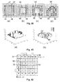
- One is able to slice a 3D volume in orthogonal planes, thus obtaining sequences of 2D images. Since a 2D image consists of pixels, the analogy can be made that each face of a voxel represents a pixel in an orthogonal slice through the volume, as shown in Fig. 1.
- Fig. 1(a) an image is shown, containing both background pixels (gray pixels 1) and foreground pixels (white pixels 2).
- the same image is shown in Fig. 1b as a slice through the volume and containing voxels, gray voxels 3 and white voxels 4.
- a pixel can be viewed as a voxel's face.
- a 3D volume can be created artificially, containing experimental or simulated data for example, or it can be the result of a stack of planar cross-sectional slices produced by an image acquisition device (e.g. MR, CT, confocal microscope, ultrasound, etc.).
- the pixels within the slices usually have the same resolution in both directions.
- the slices however, in many cases are acquired at a different resolution than the pixels within the slice, which results in an anisotropic voxel.
- some interpolation within the data set can be done in an extra pre-processing step to achieve the isotropy, or this problem can be solved at display time by applying different scaling factors, which are proportional to the voxel's resolution in ⁇ x , y , z ⁇ , for the 3D surface vertices.
- Two •-voxels are said to be strictly ⁇ -adjacent if they are adjacent only for this ⁇ .
- Two ⁇ -adjacent voxels u and ⁇ are denoted ⁇ ( u , ⁇ ) and ⁇ is called an adjacency relation.
- the transitive closure of this relation called the connectedness, is used: two •-voxels ⁇ 1 and ⁇ n are ⁇ -connected (in the set ⁇ D ) if there exists a sequence of •-voxels ⁇ 1 , ⁇ 2 ,..., ⁇ n such that for any 1 ⁇ i ⁇ n , ⁇ i is ⁇ -adjacent to ⁇ i+ 1 .
- An object O is ⁇ -connected if all pairs of voxels of O are ⁇ -connected.
- the ⁇ -neighborhood of a voxel ⁇ is a set of voxels that are ⁇ -adjacent with voxel ⁇ . Based on this definition, a more general classification of the voxels can be stated. They can be classified into three groups:
- Keppel provides a solution for building the mesh by triangulation based on randomly distributed points along contour lines.
- the number of chosen contour points depends on the desired accuracy.
- Keppel's strategy for finding the optimal arrangement of triangles approximating the unknown surface is to decompose the given set of contour points into subsets, according to their position and the shape of the contour, convex or concave, such that a proper objective function may be stated separately for each subset.
- the objective function is formulated as:
- the triangulation which maximizes the volumes of the polyhedron gives the optimal approximation of the surface provided by a pair of closed convex contour lines.
- the objective function can be extended to concave contour point sets as well.
- the optimal triangulation is found by using classical methods of graph theory.
- the main unsolved problem is the ambiguity of how to triangulate when branching structures cause splitting of one contour into several ones in the neighboring slice.
- Fuchs et al. determine the optimal surface for each pair of consecutive contours by reducing the problem of finding certain minimum cost cycles in a directed toroidal graph.
- Their algorithm has a time complexity of O ( n 2 log n ), where n is the total number of vertices on the contours bounding the triangles.
- Bajaj et al. provide a good survey of previous approaches. In their approach, Bajaj et al. tackle all three problems (correspondence, tiling and branching) simultaneously by imposing three constraints on the reconstructed surface and then deriving precise correspondence and tiling rules from these constraints. In their approach, Bajaj et al. use the 2D marching cubes algorithm as described in W.E. Lorensen and H.E. Cline, "Marching Cubes: A high resolution 3D surface construction algorithm", in M. C. Stone, editor, Computer Graphics (SIGGRAPH '87 Proceedings), volume 21, pages 163-169, 1987, to generate contour segments from an image slice.
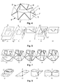
- Tiling means using slice chords to triangulate the strip lying between contours of two adjacent slices into tiling triangles 5, as shown in Fig. 4.
- a slice chord 6 connects a vertex 7 of a given contour 8 to a vertex 7' of the contour in an adjacent slice 8'.
- Each tiling triangle 5 consists of exactly two slice chords 6 and one contour segment.
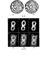
- FIG. 5(a) An example with dissimilar contours 9, 10 located on two adjacent slices is shown in Fig. 5(a).
- Fig. 5(b) shows a tiling in which all vertices of the top contour 9 tile to vertices of the bottom contour 10.
- Fig. 5(c) which is a cross section passing through the point P of the solid in Fig. 5(b) of a reconstruction as in Fig. 5(b)
- the scalar data (value) along the vertical line L flips (from outside the surface to inside, or vice versa) twice between two adjacent slices because the surface is intersected twice by L .
- This is an unlikely topology, especially when the distance between the two slices is small.
- Another tiling possibility is shown in Fig. 5(d), with the vertical cross section displayed in Fig. 5(e), in which the vertices of the dissimilar portion of the contour tile to the medial axis 11, 11' of that dissimilar portion, resulting in a highly likely topology
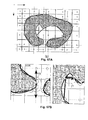
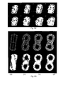
- FIG. 6(a) A top view of the two contours 9, 10 is illustrated in Fig. 6(a).
- the thicker contour is the top contour 9, and small circles represent vertices.
- the result of the minimum surface area-optimizing algorithm described in D. Meyers, "Reconstruction of Surfaces from Planar Contours", PhD thesis, University of Washington, 1994, is shown as a wire frame in Fig. 6(b) and the same in Fig. 6(c) with hidden lines removed.
- the arrow points to the abnormality where triangles intersect non-adjacent triangles.
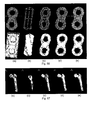
- FIG. 7 A branching problem is shown in Fig. 7, where one contour C3 of slice S2 branches into two contours C1 and C2 of slice S1 (see Fig. 7(a)).
- Figs. 7(b) and 7(c) show that a curve L or a point is added between the two slices S1, S2 to model the valley or saddle point formed by the branching.
- This method is used by Bajaj et al. and is described in C. Bajaj, E. Coyle, and K. Lin., "Arbitrary Topology Shape Reconstruction from Planar Cross Sections", Graphical Models and Image Processing, 58(6):524-543, 1996. In H.N. Christiansen and T.W.
- Branching regions that are not complex, as in the top view shown in Fig. 8(a), can be tiled by adding a vertex to model the saddle point, as shown in Fig. 8(b).
- the thicker line segments in Fig. 8(a) are top contours 9, 9', and small circles represent vertices.
- the branching contours 9, 9', 9", 10 shown in top view in Fig. 8(c) (again the thicker line segments are top contours 9, 9', 9", and small circles represent vertices), one could use line segments 13 to model canyons between the contours, as shown in Fig. 8(d).
- the surface reconstruction criteria defined by Bajaj et al. are the following:
- the correspondence rules are local (data in adjacent slices are used to determine the correspondence between contours).
- the tiling rules prohibit those undesired tilings or nonsensical surfaces, and allow detection of branching regions and dissimilar portions of contours.
- the method combines a multipass tiling algorithm that first constructs tilings for all regions not violating any of the tiling rules, and in a second and third pass, processes regions that violate these rules (holes, branching regions and dissimilar portions of contours), by tiling to their medial axes.
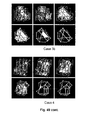
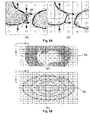
- Topologies that violate criterion 2 due to under-sampling of the original data might generate distorted results, as shown in Fig. 9, where examples of topologies are shown that cannot be processed because they violate criterion 2 by having two points of intersection with a line L perpendicular to the slice.
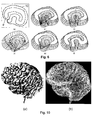
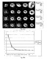
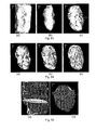
- An example of surface reconstruction of the brain hemisphere produced by the algorithm of Bajaj et al. is shown in Fig. 10. It is generated from a set of contour data that has been manually traced from 52 MRI image slices. The approach produces significantly fewer triangles than the marching cubes approach as described in W.E. Lorensen and H.E. Cline, "Marching Cubes: A high resolution 3D surface construction algorithm", in M. C.
- Fig. 10(a) represents a Gouraud shading
- Fig. 10(b) represents a wire frame of a reconstructed brain hemisphere.
- MC is based on the idea of combining interpolation, segmentation, and surface construction in one single step, but this implicit segmentation is sometimes very difficult, if not impossible, e.g. with noisy data.
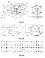
- the "original" MC algorithm as described in US-4710876 and US-4729098 is based on the tabulation of 256 different configurations, thus it falls into the category of methods that are based on a lookup table to decide how to connect the iso-surface vertices. It allows a local iso-surface extraction inside an 8-cube defined by eight voxels. The global iso-surface is the union of these small pieces of surface computed on each set of eight connected voxels of the image.
- An 8-cube as shown in Fig. 11(a), is a cube 14 lying between two image slices 15, 16 and consisting of 8 neighboring voxels (4 in each slice). A new grid is formed by identifying the image voxels as discrete 3D points. For a 3D image I with size M ⁇ N ⁇ P , there are ( M - 1)( N - 1)( P - 1) 8-cubes in I .
- the voxels, or corners, of the 8-cube 14 are either located inside (•-voxel) or outside (o-voxel) of the object 17. Whenever there are two corners with different states (inside and outside) along an edge of the 8-cube 14, there must be an intersection with the surface of the object 17.
- a lookup table with 256 entries has been generated from these 15 cases.
- the lookup table contains a list of 8-cube edge intersections with a description stating how these intersections should be connected in order to build the triangles.
- an index into the lookup is computed using the corner numbering of the 8-cube as shown in Fig. 11(b), by associating each corner with one bit in an 8-digit number, and assigning a one to each •voxel and a zero to each o-voxel belonging to the 8-cube.
- Fig. 11(b) which corresponds to case 5 of Fig.
- each triangle vertex where the iso-surfaces ⁇ intersects the 8-cube's edge, is found by linear interpolation of the density (e.g. gray value) between the edge corners.
- a unit normal is computed for each triangle vertex using the gradient information available in the 3D data.
- the gradient vector at the corners of the 8-cube is estimated and then the vectors are linearly interpolated at the point of intersection of the triangle vertices with the 8-cube edges.
- the MC algorithm has been intensively used for rendering purposes but has shown its limitations in other applications, because the extracted iso-surface is in general not a "simple" surface. Some authors have noticed that the iso-surface does not always have the same topology as an underlying continuous surface defining the image. Many authors have contributed to solve this problem, but they have often provided an empirical solution or a visual justification.
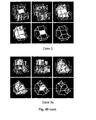
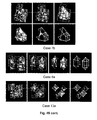
- Fig. 12 cases 3, 6, 7, 9, 10 and 13.
- Fig. 13 An example of inconsistent reconstruction of the local surface and of a correct solution are shown in Fig. 13.
- Case 6 of Fig. 12 is applied for the complementary configuration that, combined with the triangles generated by case 3, will result in holes, as triangles generated by case 3 do not match the ones generated by case 6 (actually the complement of case 6).
- a correct triangulation is shown in the right image where case 6 has been modified, a configuration that is not available in the 15 basic cases.
- a first fix to the MC algorithm is constructing iso-surfaces from CT data, as described in A. Wallin, "Constructing isosurfaces from CT data", IEEE Computer Graphics and Applications, 11 (6)28-33, November 1991.
- this method uses the 8-cube approach to extract a local surface.
- the main difference is that the configuration table is built for a 4-face instead of an 8-cube.
- the ambiguous cases found in MC are solved by using the density value (interpolated) at the center of the 4-face to determine if that point lies inside or outside the ⁇ , as described in G. Wyvill, C. McPheeters, and B. Wyvill, "Data structures for soft objects", The Visual Computer, 2:227-234, 1986.
- a polygon is a connected set of edges that forms an iso-surface.
- the ordering of a polygon is the path taken by the vertices describing it ( ⁇ 0 ⁇ ⁇ 1 ⁇ ⁇ 2 ⁇ ... ⁇ ⁇ 0 ).
- Two neighboring polygons are coherently ordered if the path of an edge shared by the two is opposite.
- a surface is coherently connected if all edges occur twice in opposite directions (two complementary edges) and if no polygon touches another polygon except at the common edge.
- the algorithm guarantees that the obtained polygons are coherently ordered and connected, with no polygon occurring more than once, and that each surface is complete, that is, no holes due to surface generation errors occur.
- the generated ⁇ consists of either the minimum number of (non-planar) polygons with 3 to 12 vertices or a minimum number of triangles.
- the surface generation process has two phases that are: the edge generation and connection, and polygon generation.
- the algorithm When one intersection occurs, the algorithm produces two edges (case 1 to 4, 6 to 9, and 11 to 14), one directed in each direction. Both of these edges must be kept in memory to produce a coherent surface later.
- the algorithm can use the (interpolated) value at the center of the face to determine if that point lies inside or outside the iso-surface, as described in G. Wyvill, C. McPheeters, and B. Wyvill, "Data structures for soft objects", The Visual Computer, 2:227-234, 1986.
- the generated surface differs slightly depending on whether the face's center is considered or not. Either way the obtained surface is valid and coherent.
- the scanning of the edges list to obtain a correct surface is more complex than the generation of edges.
- the possible polygon configurations that can be detected are triangles (one case), rectangles (two cases), pentagons (one case), hexagons (three cases), heptagons (one case), octagons (two cases), nonagons (one case), and 12 edges (two cases).
- a second fix to the MC algorithm is skeleton climbing (SC), as described in T. Poston, H.T. Nguyen, P.-A. Heng, and T.-T. Wong, "Skeleton Climbing: Fast Isosurfaces with Fewer Triangles", Proceedings of Pacific Graphics'97, pages 117-126, Seoul, Korea, October, 1997, and in T. Poston, T.-T. Wong and P.-A. Heng, "Multiresolution Isosurface Extraction with Adaptive Skeleton Climbing", Computer Graphics Forum, 17(3):137-148, September 1998.
- SC skeleton climbing
- SC uses the 8-cube approach to visit the data volume and to build triangulated iso-surfaces ( ⁇ ) in 3D grid data. It is based on a 4-step approach to construct the surface:
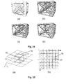
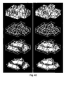
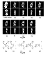
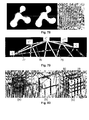
- Fig. 19 is an example of a knotted torus sampled at 64x64 resolution, whereby Fig. 19(a) is extracted by MC (13968 triangles), Fig. 19(b) is extracted by SC without step 4 (13968 triangles), and Fig. 19(c) is extracted by SC with step 4 (10464 triangles).
- SC obtains similar results as MC in terms of number of triangles, speed and visual quality, except for the cases where MC fails to correctly approximate ⁇ .
- SC with step 4 reduces the number of triangles by 25 %, and gives as a result a smoother surface, as also shown in Fig.
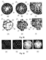
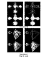
- Fig. 20 shows surfaces extracted from a 128x128x57 CT scan, with a threshold distinguishing bone from non-bone.
- Fig. 20(a) is extracted by MC (100830 triangles)
- Fig. 19(b) is extracted by SC without step 4 (100066 triangles)
- Fig. 19(c) is extracted by SC with step 4 (75318 triangles).
- SC with step 4 gives a smoother forehead region, and equally good detail.
- the triangular mesh is generated from these boxes instead of the cubes as in SC.
- the coarseness of the generated meshes is controlled by a specified maximum size ( N ) of the boxes.
- N 1, the largest box contains 2x2x2 voxels, like in MC.
- the proposed on-the-fly triangle reduction approach can generate meshes that are more accurate because it directly makes use of the voxel values in the volume.
- the algorithm has the advantage that the construction of coarser iso-surfaces requires less computation time, which is contrary to mesh optimization approaches, generally requiring a longer time to generate coarser meshes.
- ASC allows the user to obtain rapidly a low-resolution mesh for interactive preview purposes and to delay the decision for the more time-consuming generation of the detailed high-resolution mesh until optimal parameter settings (threshold, viewing angle, ...) have been found.
- ASC is much faster than post-processing triangle reduction algorithms. Therefore, the coarse meshes ASC produces can be used as the starting point for mesh optimization algorithms, if mesh optimality is the main concern. Similar to SC, ASC does not suffer from the gap-filling problem.
- the adjacency relation can be specified for both •-voxel and o-voxel, call it ⁇ respectively ⁇ .
- the orientation of the polygon's edge is important in defining the orientation of the surface.
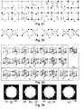
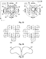
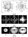
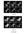
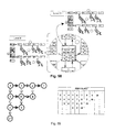
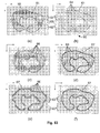
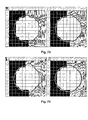
- the concept of the orientation of the edges is demonstrated in Fig. 21 for the 16 cases of a 4-face, while the generalization for the 8-cube is shown in Fig. 23.
- the inner part of the surface (see Fig. 21), displayed in gray, is located on the left side of the oriented edge. Two cases (case 5 and 10) are ambiguous, and the choice of the right connectedness couple ( ⁇ , ⁇ ) is essential.
- Fig. 23 The modified MC configurations for the 14 cases and the valid connectedness couples are shown in Fig. 23. Similar to original MC, cases that can be obtained via rotation or symmetry are not displayed.
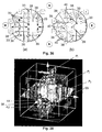
- Fig. 24(a) displays a 3D surface rendering of the individual voxels, whereby each voxel is shown as a box.
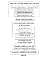
- the present invention relates to four related but independent aspects: (1) an embodiment (called for brevity's sake TriScanTM) providing a method and a system to derive mesh surface descriptions (also called connectivity-wireframes) from objects represented as a scalar field (e.g. discrete multi-dimensional data), scalar functions (e.g.
- TriScanTM and MeshGridTM terminologies are used to make the distinction between two concepts, namely the surface structure extraction and the surface structure representation in the form of a combined surface mesh description attached to a reference grid, however these terms are not limiting on the invention. It should be understood that the terms TriScanTM and MeshGridTM are each shorthand for a series of embodiments of the present invention.
- the TriScanTM method is a surface extraction method that generates a surface description in discrete mesh form, called a connectivity-wireframe for convenience sake, whch can be stored. It can optionally be brought to a grid representation to form a combined surface mesh description attached to a reference grid, e.g. the MeshGridTM representation.
- the connectivity-wireframe obtained with TriScanTM comprises a set of connected vertices or nodes, and for each vertex its (typically four) neighbors and its coordinates are specified.
- the connectivity-wireframe obtained with TriScanTM may contain for each vertex extra information, such as: a discrete border direction and an appropriate discrete position given by the indices of the sections cutting through the object, defining the discrete grid of points, the reference-grid.
- the MeshGridTM representation exploits the fact that each discrete position of the reference-grid has its own coordinates and that a vertex of the surface mesh representation can be attached to its appropriate discrete position in the reference grid by specifying a scalar offset for each vertex instead of its coordinates in the grid.
- a vertex is located on the grid-segment connecting two grid-points (discrete positions), and the vertex offset is a number, preferably between 0 and 1, preferably specifying the relative position of the vertex on that grid-segment.
- the coordinate of a vertex can be expressed as the coordinates of the discrete position to which it is attached to, plus an offset vector defined as the multiplication between the scalar offset and the vector of the grid-segment defined in the direction of the border.
- a MeshGridTM representation is independent of the TriScanTM method and can be used with a surface meash representation of a an object obtained by other means than the TriScanTM method. Any mesh can be attached to a reference-grid, but for efficient coding the mesh should follow the same connectivity constraints as imposed by the TriScanTM method.
- the representation of MeshGridTM can be stored, e.g. on a CD-ROM or hard drive of a general purpose computer or transmitted to a remote location.
- One aspect of the invention includes a method of deriving and preparing data for display of a n-1 dimensional surface description in the form of a mesh, called a connectivity-wireframe, of an n-dimensional object, n being at least 3, the surface mesh description to be derived by the method comprising a plurality of boundary nodes (or vertices), each boundary node lying on or adjacent to the surface to be described, each boundary node being associated with connectivity information.
- the connectivity information can comprise representations of up to (n-1) incoming and/or (n-1) outgoing directions towards 2*(n-1) adjacent boundary nodes adjacent to the said boundary node, the orientation of the incoming or outgoing directions being defined in such a way that the cross product of the up to (n-1) incoming directions or (n-1) outgoing directions associated with any boundary node gives a vector which points away from the surface at that boundary node.
- a polygonal representation may be generated from the connectivity-wireframe of the object, e.g. from the plurality of boundary nodes and the connectivity information of those boundary nodes.
- the step for obtaining the mesh representation of the surface, i.e. the connectivity-wireframe, from an n-dimensional object can comprise defining n sets of (n-1)-dimensional reference-surfaces; the reference-surfaces of one set keeping their initial ordering at the surface of the object. Typically (at least during generation of the representations), no two reference surfaces of one set will intersect within the object and no single reference surface intersects itself within the object.
- Another step for obtaining the connectivity-wireframe from an n-dimensional object comprises determining contours of the surface, each contour lying in a reference surface of n-1 lower dimensions.
- a contour can be defined as an iso-contour of a physical property of the object.
- the property may be the gray level, for example.
- the iso-contours are defined by at least two values of the property (e.g. -1, 1), i.e. a value labeling the inside of the object, and a value labeling the outside of the object for the specified property.
- a third value of the property (e.g. 0), i.e. the value identifying the precise position of the border for the specified property for the object.
- the third value of the property improves the precision of the contouring of the object with respect to the specified property.
- a polygonal representation of the surface of the object is obtained from the connectivity information of the connectivity-wireframe.
- the polygonal representation of the surface of the object consists of a union of a set of surface primitives.
- the surface primitives are identified from the connectivity information of the connectivity-wireframe on the bases of a set of connectivity rules.
- the method comprises rendering the surface from the polygonal representation.
- the rendered surface can then be displayed.
- intersection points of n sets of further reference-surfaces define a grid called the reference-grid.
- a reference-grid point has a coordinate and it can be identified by the indices of the reference-surfaces intersecting in that point.
- the boundary node description contains at least the coordinates of a vertex of the mesh representation and the connectivity to other boundary nodes.
- the boundary node description may contain in addition the direction vector of the border and the position of a reference-grid point, identified by the indices of the reference-surfaces intersecting in that point; the reference-grid point the boundary node is referring to, is located inside or outside the object, closest to the boundary node in the direction of the border specified for the boundary node.
- the connectivity-wireframe obtained from the TriScanTM method can further be decomposed into a hierarchical or non-hierarchical multi-resolution representation; the highest resolution of the connectivity-wireframe can be imposed identical with the initial non multi-resolution connectivity-wireframe.
- the hierarchical feature of the multi-resolution connectivity-wireframe implies that any boundary node from a lower resolution connectivity-wireframe will be found in all the higher resolution connectivity-wireframes.
- the connectivity information associated with the boundary node may change between successive resolutions of the connectivity-wireframe.
- the step in building the hierarchical or non-hierarchical multi-resolution connectivity-wireframe consists in obtaining successive lower resolution connectivity-wireframe from an immediate higher connectivity-wireframe by removing some of the reference-surfaces of the immediate higher connectivity-wireframe.
- a different approach in building the hierarchical or non-hierarchical multi-resolution connectivity-wireframe consists in obtaining successive higher resolution connectivity-wireframes from an immediate lower connectivity-wireframe by adding some of the reference-surfaces to the immediate lower connectivity-wireframe.
- hierarchical multi-resolution connectivity-wireframes may consist of at least one hierarchical node description to a plurality of other hierarchical node descriptions.
- the hierarchical node description is a node description that has associated a hierarchical connectivity information comprising representations of up to (n-1) incoming and (n-1) outgoing directions towards 2*(n-1) adjacent boundary nodes adjacent to the said boundary node, for each resolution of the connectivity-wireframe the said boundary node exists.
- the connectivity-wireframe obtained with the TriScanTM method can be stored as it is.
- the present invention also includes a system for carrying out the above methods as well as a computer program product which when executed on a computing device executes one or more of the above methods, i.e. includes code segments able to execute one of the above methods.
- the present invention also includes the computer program product stored on a suitable data carrier, which when inserted into a computing device exexcutes one of the above methods.
- Another aspect of the invention is a compact, optionally multi-scalable, optionally view-dependent, optionally animation-friendly multi-dimensional surface representation method - called MeshGridTM which is a combination of a reference grid and a surface mesh representation of an object (connectivity wireframe) attached thereto in which connectivity information is provided.
- MeshGridTM is a combination of a reference grid and a surface mesh representation of an object (connectivity wireframe) attached thereto in which connectivity information is provided.
- Yet another aspect of the invention is the representation of the TriScanTM connectivity-wireframe in the MeshGrid representation.
- the step for obtaining the MeshGridTM representation, of the surface of an n-dimensional object comprises specifying n sets of reference-surfaces; the reference-surfaces of one set keeping their initial ordering at the surface of the object.
- Another step for obtaining the MeshGridTM representation, of the surface of an n-dimensional object comprises deriving a surface mesh description (the connectivity-wireframe) of the object having specific connectivity properties.
- a connectivity-wireframe can be obtained using the TriScan method.
- a polygonal surface mesh representation may be used, e.g. a quadrilateral mesh having, e.g. a 4-connectivity property of the connectivity-wireframe, yet the connectivities between the mesh vertices have to be rearranged to the specificity of the connectivity-wireframe.
- Yet another step of obtaining the MeshGridTM representation, of the surface of an n-dimensional object comprises obtaining the reference-grid description of the n-dimensional object, the reference-grid being defined by the intersection points of the specified reference-surfaces.
- Yet another step of obtaining the MeshGridTM representation, of the surface of an n-dimensional object comprises defining the offsets for the boundary nodes of the connectivity-wireframe.
- a boundary node will be attached to a reference-grid point, identified by the indices of the reference-surfaces intersecting in that point; the boundary node may be located on the grid-line segment connecting the reference-grid point it is attached to, with another reference-grid point.
- the offset of a boundary node is computed in relation with the reference-grid point it is attached to, and offset calculation may yield any value preferably between 0 and 1, including 0; in this case the offset is preferably defined as a relative value.
- the method consists in attaching the connectivity-wireframe of a n-dimensional object to the reference-grid and storing a plurality of boundary node descriptions, each description being at least a definition of an intersection point in the grid and an associated offset.
- a MeshGrid representation consists of at least one boundary node, defined by a reference-grid point and an offset.
- the coordinate of a boundary node can be expressed as the coordinates of the reference-grid position to which it is attached to, plus an offset vector defined as the multiplication of the scalar offset and the vector of the grid-segment, the boundary node is located on, defined in the direction of the border.
- the polygonal representation of the surface of the n-dimensional object is obtained from the connectivity information of the connectivity-wireframe attached to reference-grid in the MeshGrid representation.
- the surface description of a n-dimensional object is defined in the MeshGrid representation via a connectivity-wireframe comprising the description of the boundary nodes, and via the reference-grid description comprising the reference-grid points.
- the connectivity-wireframe is the connectivity layer that can be attached to a plurality of reference-grid descriptions compatible with the reference-surfaces used to generate the surface-description, respectively the connectivity-wireframe (e.g. different compatible reference-grid descriptions can be obtained when deforming or animating an existing reference-grid).
- the reference-grid description gives the volumetric or spatial distribution of an object.
- Another aspect of the invention is the MeshGrid representation of surface descriptions different from the ones obtained via the TriScan method.
- other polygonal meshes such as Qadrilateral meshes, may be stored in the MeshGrid representation.
- the step of obtaining a MeshGrid representation from a polygonal mesh such as a quadrilateral mesh comprises defining a constrained reference-grid based on the number of polygons e.g. quadrilaterals, in the mesh.
- Another step for obtaining a MeshGrid representation from a polygonal mesh may comprise deforming or uniformly distributing the reference-grid to fit the volume of the polygonal mesh, e.g. quadrilateral mesh; the vertices of the polygonal mesh, e.g. quadrilateral mesh, can be used as boundary conditions for the distribution of the reference-grid points.
- Yet another step for obtaining a MeshGrid representation from a polygonal mesh comprises deriving the connectivity information between the vertices of the polygonal, e.g. quadrilateral mesh, to build the mesh description.
- Yet another step for obtaining a MeshGrid representation from a polygonal mesh, e.g. a quadrilateral mesh comprises attaching the vertices of the polygonal, e.g. quadrilateral mesh to reference-grid points, and specifying the offset for each vertex.
- the reference-grid points can be distributed in such a way that the vertices or the boundary nodes lie at an arbitrary position, e.g. at half the distance, between two grid points, thus yielding an offset of 0.5, the default value, which does not need to be stored.
- the MeshGrid representation may have a hierarchical multi-resolution structure.
- the highest resolution MeshGrid representation contains all the reference-grid points.
- the hierarchical feature of the multi-resolution MeshGrid representation implies that any reference-grid point from a lower resolution MeshGrid representation will be found in all the higher resolution MeshGrid representations. Consequently the mesh description attached to the reference-grid in the hierarchical MeshGrid representation will follow the same hierarchical description.
- the step in building the hierarchical multi-resolution MeshGrid representation consists in obtaining successive lower resolution MeshGrid representations from an immediate higher MeshGrid representation by removing some of the reference-surfaces or the equivalent reference-grid points of the immediate higher MeshGrid representation.
- a different approach in building the hierarchical MeshGrid representation consists in obtaining successive higher resolution MeshGrid representations from an immediate lower MeshGrid representation by adding some of the reference-surfaces or the equivalent reference-grid points to the immediate lower MeshGrid representation.
- the reference-surface spacings may be changed locally or globally to provide re-sizing of the surface mesh or, for instance, animation.
- Reference surfaces may touch each other or pass through each other in these circumstances. Parts of the mesh may be "cut" or deformed.
- three types of scalability can be exploited simultaneously in progressive transmission schemes with variable detail that depend on the bandwidth of the connection and the capabilities of the terminal equipment, in both view-dependent and view-independent scenarios.
- the view-dependent scenario is implemented by means of regions-of-interest (ROIs).
- ROI is defined as a part of the reference-grid.
- ROI based coding implies subdividing the entire MeshGrid in smaller parts and encoding the connectivity-wireframe and reference-grid description of each of these parts separately.
- the three types of scalability are: (1) mesh resolution scalability, i.e. adapting the number of transmitted vertices on a ROI basis in view-dependent mode or globally otherwise, and (2) shape precision i.e.
- the MeshGrid representation supports specific animation capabilities, such as (1) rippling effects by changing the position of the vertices relative to corresponding reference-grid points (the offset), and (2) reshaping the regular reference-grid and its attached vertices, which can be done on a hierarchical or non-hierarchical basis;
- any changes applied to the reference-grid points, corresponding to a lower resolution of the mesh will be propagated to the reference-grid points, corresponding to the higher resolutions of the mesh, while applying a similar deformation to the reference-grid points corresponding to a higher resolution of the mesh will only have a local impact.
- each vertex will retrieve its 3D coordinates from the coordinates of the grid points it is attached to, and from the specified offset.
- the present invention also includes a system for carrying out the above methods as well as a computer program product which when executed on a computing device executes one or more of the above methods.
- the present invention also includes the computer program product stored on a suitable data carrier.
- the method comprises transmitting a combined surface mesh representation with a reference grid attached thereto, e.g. the MeshGrid representation, of the surface to a remote location.
- the transmission step comprises the step of generating a bit-stream from the combined, e.g. MeshGrid representation.
- the bit-stream will in general consist of three parts: (1) a description of the mesh describing the surface, i.e. the connectivity-wireframe description, (2) optionally, a reference-grid description, and (3) optionally, a vertices (node)-refinement description (i.e. refining the position of the vertices relative to the reference-grid - the offsets).
- a description of the mesh describing the surface i.e. the connectivity-wireframe description
- a reference-grid description optionally, a vertices (node)-refinement description (i.e. refining the position of the vertices relative to the reference-grid - the offsets).
- Each of these parts can be specified according to the type of bit-stream in single-resolution, multi-resolution, view-dependent or view-independent modes.
- a minimal bit-stream may however only consist of the description of the connectivity-wireframe, which is mandatory for every stream. In that case the 8 corners of the reference-
- this reference-grid As an aspect of the invention, due to its regular nature, it is possible to divide this reference-grid into a number of 3D blocks (called ROIs), and it is possible to encode the surface locally in each of these ROIs.
- the ROIs are defined in such a way such that the entire volume is covered. Two ROIs may share a face but they do not overlap.
- the view-dependent coding consists in coding the MeshGrid representation for each ROI independently.
- the coding of the single-resolution connectivity-wireframe consists of coding of at least one boundary node and the connectivity information of a plurality of boundary nodes as a list of directions starting from at least one boundary node to reach the plurality of other boundary nodes.
- the coding of a multi-resolution connectivity-wireframe in a bit-stream consists of coding each resolution of the connectivity-wireframe separately in the bit-stream.
- the connectivity-wireframe is split into regions of interest (ROI) and the description of the connectivity-wireframe from each ROI is coded separately, consisting of at least one boundary node and the connectivity information of a plurality of boundary nodes as a list of directions starting from at least one boundary node to reach the plurality of other boundary nodes.
- ROI regions of interest
- each resolution of the multi-resolution connectivity-wireframe can be coded either in a view-independent or view-dependent way.
- the coding of the single-resolution reference-grid description consists of coding the description of the n sets of reference-surfaces; the reference-surfaces keep their initial ordering at the surface of the object, and they do not self-intersect.
- the coding of the multi-resolution reference-grid description in a bit-stream consists of coding each resolution of the reference-grid description separately in the bit-stream.
- the reference-grid description is split into regions of interest (ROI) and the reference-grid description from each ROI is coded separately.
- ROI regions of interest
- each resolution of the multi-resolution reference-grid description can be coded either in a view-independent or view-dependent way.
- the generating step includes obtaining from the offset of each boundary node a set of refinement bits.
- each refinement bit is one of a set of discrete values that may include zero.
- the refinement values are a set of successively diminishing values, e.g. a set of relative values between 0 and 1 whereby at least one value, e.g. 0.5 may be omitted as an assumed default value.
- the coding of the single-resolution vertices-refinement description consists of coding of at least one offset corresponding to a boundary node.
- the coding of the multi-resolution vertices-refinement description in a bit-stream consists of coding each resolution of the vertices-refinement description separately in the bit-stream.
- the vertices-refinement description is split into regions of interest (ROI) and the description of the vertices-refinement description from each ROI is coded separately, consisting of at least one offset corresponding to a boundary node.
- ROI regions of interest
- each resolution of the multi-resolution vertices-refinement description can be coded either in a view-independent or view-dependent way.
- the method comprises transmitting a bit-stream.
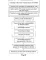
- the method comprises decoding the bit-stream and generating the polygonal representation.
- the view-independent scenario consists of decoding all the view-dependent information for a certain resolution level, while in the view-dependent scenario, one can retrieve the description of parts from a certain resolution level and decode them.
- different parts of the recovered combined surface mesh representation attached to the reference grid e.g. MeshGrid
- single resolution decoding relies on locating the appropriate resolution level of the MeshGrid description in the stream and decoding it.
- the decoding will start at a certain resolution level (it does not have to be the first resolution level) and continue from that level on till a certain higher resolution level. This approach is very different from classical multi-resolution representations that typically need the decoding of the lower resolution versions of a mesh, before being able of enhancing some portions of it by incrementally decoding additional parts of the bitstream.
- a minimal stream may however only consist of the description of the surface mesh representation with connectivity information, i.e. the connectivity-wireframe, which is mandatory for every stream.
- connectivity information i.e. the connectivity-wireframe
- a default equally distributed reference-grid, upon which the MeshGrid is based, can be derived from its 8 corners that where specified in the header of the stream.
- the method comprises initializing a reference-grid at a first resolution, by reading at least the description of the eight corners, for instance.
- the method comprises initializing the MeshGrid from the reference-grid description and from the representation of an empty connectivity-wireframe.
- the method comprises initializing the connectivity-wireframe by reading the connectivity information of a first number of boundary nodes, and initializing nodes of the connectivity-wireframe in accordance with the connectivity information.
- the minimal information that has to be read for the connectivity information for decoding is the description of a single connectivity information from one node to another.
- the state of the decoding of the connectivity-wireframe has to be kept between successive reading and decoding steps. The state has no longer to be kept when the entire connectivity information belonging to a certain resolution level of the connectivity-wireframe, in view-independent mode, or to a certain region of interest of the connectivity-wireframe, in view-dependent mode, has been read.
- the minimal information that has to be read for the reference-grid description for decoding is the description of a update for a single reference-grid point.
- the state of the decoding of the reference-grid has to be kept between successive reading and decoding steps. The state has no longer to be kept when the entire description of the reference-grid belonging to a certain resolution level, in view-independent mode, or to a certain region of interest, in view-dependent mode, has been read.
- the method comprises receiving a progressive description of the n sets of reference-surfaces for updating the reference-grid of the MeshGrid representation.
- This description may contain the information for the entire resolution level of the reference-grid, or a local information to update the reference-grid inside a region of interest (for view-dependent decoding).
- the method allows the progressive refinement of the reference-grid such that a lossy to lossless reconstruction of the coordinates of the reference-grid points is feasible.
- the progressive refinement of the reference-grid can be done for the reference-grid points of a certain resolution level, in view-independent mode, or to a certain region of interest, in view-dependent mode.
- the method allows to refine the coordinates of the reference-grid points of the higher resolution levels based on the coordinates of the reference-grid points from lower resolution levels by means of interpolation methods.
- the method comprises receiving a description of a connectivity-wireframe to a higher resolution level, consisting of at least one boundary node description to a further set of boundary nodes, and initializing a further set of boundary nodes in the connectivity-wireframe (and MeshGrid) to allow a higher resolution display of the surface.
- the method comprises receiving connectivity information of a second number of boundary nodes and a definition of the used reference surfaces, and initializing a further set of boundary nodes in the connectivity-wireframe MeshGrid to allow a higher resolution display of the surface.
- the method comprises receiving a progressive description of the vertices' refinement bits (the offset) for at least one boundary node.
- This description may contain the information for all the nodes of the connectivity-wireframe at a certain resolution level, in view-independent mode, or only for those nodes lying inside a region of interest, in view-dependent mode.
- the minimal information that has to be read for the vertices' refinement description for decoding is the description of a update for a single node from the connectivity-wireframe.
- the state of the decoding of the reference-grid has to be kept between successive reading and decoding steps. The state has no longer to be kept when the entire vertices' refinement description belonging to a certain resolution level, in view-independent mode, or to a certain region of interest, in view-dependent mode, has been read.
- the method comprises generating a polygonal representation from the decoded connectivity-wireframe of the object.
- the method comprises obtaining surface primitives from the polygonal representation of the surface.
- Another aspect of the invention includes a system for preparing data for displaying a surface of an n-dimensional body, n being at least 3, the system comprising means for providing an n-dimensional discrete mesh representation of the surface, the mesh representation comprising a plurality of boundary nodes, each boundary node lying on or adjacent to the surface, each boundary node being associated with connectivity information and means for generating a polygonal representation of the surface of the object from the plurality of boundary nodes and the connectivity information of those boundary nodes.
- the connectivity information may comprise representations of up to (n-1) incoming and/or (n-1) outgoing directions towards 2*(n-1) adjacent boundary nodes adjacent to the said boundary node, the directions being defined in such a way that the cross product of the up to n-1 incoming or outgoing directions associated with any boundary node represents a further vector which points away from the surface at that boundary node.
- the means for obtaining a mesh representation of the surface comprises means for obtaining a reference-grid description of the n-dimensional body, the reference-grid being defined by the intersection points of n sets of reference surfaces; the reference-surfaces keep their initial ordering at the surface of the object, and they do not self-intersect.
- the system comprises means for changing the spacing between the reference-grid points locally or globally to provide resizing and reshaping of the surface or, for instance, animation; reference-surfaces may touch each other or pass through each other in these circumstances. Parts of the mesh may be "cut" or deformed.
- the system allows means for three types of scalability simultaneously in progressive transmission schemes with variable detail that can depend on the bandwidth of the connection and the capabilities of the terminal equipment, in both view-dependent and view-independent scenarios.
- the view-dependent scenario is implemented by means of regions-of-interest (ROIs).
- ROI is defined as a part of the reference-grid.
- ROI based coding implies means for subdividing the entire MeshGrid in smaller parts and encoding the connectivity-wireframe and reference-grid description of each of these parts separately.
- the three types of means for scalability are: (1) means for mesh resolution scalability, i.e.
- the means for animation are provided, such as (1) means for rippling effects by changing the position of the vertices relative to corresponding reference-grid points (the offset), and (2) means for reshaping the regular reference-grid and its attached vertices, which can be done on a hierarchical or non-hierarchical basis.
- the system is adapted so that when reshaping or animating the reference-grid on a hierarchical basis, any changes applied to the reference-grid points, corresponding to a lower resolution of the mesh, will be propagated to the reference-grid points, corresponding to the higher resolutions of the mesh, while applying a similar deformation to the reference-grid points corresponding to a higher resolution of the mesh will only have a local impact.
- the means for the vertex-based animation further includes means for each vertex to retrieve its 3D coordinates from the coordinates of the grid points it is attached to and from the specified offset.
- system further comprises means for generating a bit-stream from at least one boundary node and the connectivity information of a plurality of boundary nodes as a list of directions starting from at least one boundary node to reach the plurality of other boundary nodes.
- the system includes a bit-stream coder, coding an n-dimensional discrete mesh representation of a surface, the mesh representation of the surface comprising a plurality of boundary nodes, each boundary node lying on or adjacent to the surface, each boundary node being associated with connectivity information.
- the connectivity information may comprise representations of up to n-1 directions towards n-1adjacent boundary nodes adjacent to the said boundary node, the directions being defined in such a way that the cross product of the up to n-1 directions associated with any boundary node represents a further vector which points away from the surface at that boundary node; the reference-grid being defined by the intersection points of n sets of reference surfaces; the reference-surfaces keep their initial ordering at the surface of the object, and they do not self-intersect.
- the bit-stream may comprise a representation of at least one boundary node and the connectivity information of a plurality of boundary nodes as a list of directions starting from at least one boundary node to reach the plurality of other boundary nodes. in addition the bit-stream may comprise the description of the reference-grid, and the description of vertices' refinement information.
- the system comprises a decoder for receiving a data bit-stream representing a surface of an n-dimensional body, n being at least 3, comprising means for receiving a bit-stream comprising a representation of n sets of reference surfaces, one set comprising a plurality of reference surfaces for one of the n dimensions, the reference-surfaces keeping their initial ordering at the surface of the object, and they do not self-intersect.
- the system comprises a representation of at least one boundary node, and connectivity information as a list of directions starting from at least one boundary node to reach a plurality of other boundary nodes, means for initializing an n-dimensional reference-grid at a first resolution, means for reading the representation of at least one boundary node, means for reading the connectivity information of a first number of boundary nodes and for initializing nodes of the connectivity-wireframe in accordance with the connectivity information.
- the decoder further comprises means for receiving a description with one boundary node, that may already exist in the connectivity-wireframe description of a lower or current resolution level, to a description of a further set of boundary nodes, that may already exist in the connectivity-wireframe description of a lower or current resolution level, and means for initializing a further set of boundary nodes in the connectivity-wireframe, to allow a higher resolution display of the surface.
- the decoder further comprises means for receiving connectivity information of a second number of boundary nodes and a definition of the used reference-surfaces, and means for initializing a further set of boundary nodes in the connectivity-wireframe to allow a higher resolution display of the surface.
- the system comprises a method for generating a connectivity-wireframe of the surface, the connectivity-wireframe comprising a set of boundary nodes defined by intersection points in the reference-grid and offsets from this grid.
- the system comprises a method for obtaining a polygonal representation of the surface from the connectivity-wireframe; the polygonal representation consisting of the union of a set of surface primitives.
- the system comprises a method for rendering the surface from the union of the surface primitives.
- the system comprises a method for receiving in the bit-stream for at least one reference-grid point, an update description, and modifying the coordinates of those reference-grid points.
- the system comprises a method for progressive refinement of the coordinates of a reference-grid point by successively reading a larger part of the reference-grid description.
- the system comprises a method for receiving in the bit-stream for at least one node, a refinement description, and modifying the position of at least one boundary node relative to the reference-grid in accordance with at least a part of the vertices' refinement description.
- the system comprises a method for progressive refinement of the position of the boundary node relative to the reference-grid by successively reading a larger part of the vertices' refinement description.
- the present invention discusses three related topics: (1) a method - called TnScanTM - which is an embodiment of the present invention - to acquire surface descriptions from a plurality of sections through multi-dimensional representations of objects, especially through the three-dimensional representations of objects (2) a compact, optionally multi-scalable, optionally view-dependent, optionally animation-friendly multi-dimensional surface representation method - called MeshGridTM which is also en embodiment of the present invention - of these surface descriptions and the digital coding of the MeshGridTM surface representation (3) and the conversion of other surface descriptions to the MeshGrid surface representation which are also embodiments of the present invention.
- the object can be expressed as a scalar field (e.g. discrete multi-dimensional data), scalar functions (e.g. implicit surfaces) or any other surface description that is different from the surface description obtained by the TriScanTM method.
- volumetric data discrete representation of objects
- principle upon which the method works can as well be applied to objects defined, for example, in a continuous space (analytical representation of objects).
- the idea behind the TriScanTM method of the present invention is to retrieve a surface description in the form of a mesh, which, for convenience only, is called the 3D connectivity wireframe, of an object such that a polygonization of the surface description can be derived, preferably without ambiguity, from the its connectivity information.
- the obtained polygonal representation of the object's surface comprises a union of surface primitives such as: triangles, quadrilaterals, pentagons, hexagons and heptagons.
- the resulting surface is closed and without self-intersections and it respects the topology of the underlying object. No surface primitives overlap, and there are no holes in the final surface.
- the surface is the complementary of the surface obtained from the inverse object.
- the algorithm is fully automatic, although some user interaction is not excluded to identify the initial position of the object as explained hereinafter. Its applicability goes beyond plain rendering: i.e. the algorithm can be exploited for structure and finite element analysis.
- the approach of such a method of the present invention can be classified in the category of contour oriented surface extraction methods.
- the TriScan method of the present invention will be explained in the context of the discrete and continuous 3D space but it can be generalized to an n-dimensional space as well.
- the surface description has a regular structure, since each vertex from the connectivity-wireframe is connected to 4 other vertices. Each vertex is located on the estimated surface of an object. Any vertex knows which are its 4 neighbors in two perpendicular paths given by the direction of the reference-surfaces, explained later, passing through those vertices. Moreover, the path followed by migrating from one vertex to its neighbor, always in the same direction, will finally close. Therefore it is concluded that from each vertex one can navigate to any other vertex inside the same connectivity-wireframe. Using this architecture one is able to store besides the coordinates of the vertices, positioned on the object's surface, the connectivity information between them.
- the surface primitives are aimed to fill in the openings in the connectivity-wireframe (the patches), one surface primitive for each patch.
- a set of rules has been designed that use the connectivity information from the surface description to track and identify an opening, and then generate the surface primitive that fits into it. Since each vertex has 4 distinct neighbors, and a patch has in average 4 nodes, the total number of patches and implicitly the number of surface primitives will approximately be equal to the number of vertices from the connectivity-wireframe.
- the surface extraction algorithm of the present invention is a contour oriented method since it describes the surface of an object as a connected frame of vertices. When applied to the 2D space, the method generates (a) contour(s), thus by adding an extra dimension a connectivity-wireframe is obtained. Since the approach is based on deriving contours from an object and on the geometrical properties of these contours, the following definitions may be used:
- the connectivity-wireframe approximates the "real" surface of the object with a certain precision that depends on the number of vertices in the surface description (the resolution) and their distribution. Therefore a slicing set-up is needed to impose the positions where the information about the object's surface is required.
- the slicing set-up can be visualized as 3 sets of reference-surfaces. Each reference-surface has a certain ordering inside the set. The reference-surfaces from one set keep their ordering at the surface of the object, and do not self-intersect. The reference-surfaces from one set intersect the reference-surfaces from the other sets.
- intersection of these reference-surfaces define a 3D grid of points, and the distance between two grid points define the slicing step(s) in the 3 sets of reference-surfaces.
- these 3 sets of reference-surfaces are mutually perpendicular, and each reference-surface is planar.
- the strategy applied to generate the surface-description is conditioned by the way the objects are defined (i.e. discrete or continuous space) and represented (e.g. voxel mode, f(x,y,z), analytical contours).
- the objects are defined (i.e. discrete or continuous space) and represented (e.g. voxel mode, f(x,y,z), analytical contours).
- f(x,y,z) For discrete objects or in case their surface can be expressed as a function f(x,y,z), one could design a border-tracking algorithm that makes the contouring of the object for the positions specified in the slicing set-up.
- the border-tracking algorithm would use a decision function, which computes some property of the object (e.g. gray level of the voxel, evaluate f(x,y,z)), to locate the position of the boundary.
- the surface extraction method can be applied on objects defined by analytical contours as well.
- Each contour has to be defined as a series of connected vertices. Since the resolution of the resulting contours is usually much higher than imposed by the slicing set-up, some of the vertices that do not satisfy some connectivity constraints have to be removed as described later.
- the reference-surfaces are considered to be planar, the 3 sets are mutually perpendicular, and the normal direction of the reference-surfaces are aligned to the axes of the orthogonal coordinate system, although the same conclusions are obtained when employing non planar, non-orthogonal reference-surfaces.
- the TriScanTM method of the present invention has the advantage that different resolutions of the object can be obtained by choosing different slicing steps within or between perpendicular slices through the object, this for both continuous and discrete spaces.
- Irregular slicing steps through the object may improve the approximated model by selecting the most appropriate positions to cut the object into slices (e.g. where the shape of the object changes dramatically, or in areas with high curvature).
- An example of a connectivity-wireframe approximating a continuous, respectively discrete sphere, obtained with an irregular slicing step in the first case, respectively a regular slicing step in the second case, is shown in Fig. 28. The multi-resolution issues are discussed later.
- the TriScanTM method of the present invention will be explained in what follows by means of discrete models, because the whole procedure of the TriScan method, including the border-tracking engines, was primarily designed to work on discrete volumetric models. Another reason is that it is much more intuitive to explain the method on discrete objects, than on continuous objects. However, it is to be kept in mind that the TriScan method of the present invention can also be applied on models defined in the continuous space.
- each voxel 19 is represented as a cube of unit size and, consequently, has its own faces and edges.
- Voxel ⁇ situated at position (i,j,k) in the 3D grid has the coordinates of its center 20 at (i+0.5,j+0.5,k+0.5). There is no distance between adjacent voxels.
- Two 6-adjacent voxels share a face
- two 18-adjacent voxels may share a face or an edge
- two 26-adjacent voxel may share a face, an edge or a vertex (see also Fig. 2).
- Voxel 19 is delimited by six planes of coordinates ⁇ i, i+1, j, j+1, k, k+1 ⁇ .
- Each of the six faces of a voxel ⁇ k is shared with another voxel ⁇ l that is 6-adjacent with ⁇ k .
- a face shared between a background voxel (o-voxels) and a foreground or object voxel (•-voxels) is called a border face.
- a slice through the volume is taken.
- a 2D adjacency model for a slice can be specified, as shown in Fig. 26.
- the correspondence of the 6-connectivity in 3D, as shown in Fig. 2(a) is the 4-connectivity in 2D, as shown in Fig. 26(a).
- the 18-connectivity in 3D, as shown in Fig. 2(b) corresponds to the 8-connectivity in 2D, as shown in Fig. 26(b).
- the shape of a contour extracted from a slice through the object depends on the 2D, respectively 3D connectivity model chosen when tracking the object's border.
- the 2D contouring both 4 and 8-connectivity models can be used, while for the 3D approach the 6 and 18-connectivity model can be implemented, and is preferred because it is based on three 2D mutually perpendicular scans.
- the influence of different connectivity models on the resulting connectivity-wireframe can be noticed.
- the 4-connectivity (2D approach) respectively the 6-connectivity (3D approach) model was used.
- a slightly different shape, in Figs. 27(c) and (d) was generated when the 8-connectivity (2D approach), respectively the 18-connectivity (3D approach) was used instead.
- FIG. 28 An example of surfaces extracted with the TriScan method of the present invention from a sphere defined in the continuous and discrete space is shown in Fig. 28.
- An image space containing a sphere (Figs. 28(a) and (c)) is sliced in three mutually perpendicular directions, and the borders are contoured for each slice.
- a variable step is used for slicing the continuous version of the sphere 21 of Fig. 28(a), and a constant step for slicing the discrete version of the sphere 22 of Fig. 28(d).
- the slices and contours are indicated by 25, 26, 27, one number for each reference-surface. Vertices are displayed as dots 23 in Figs. 28(b) and (e) and result from the intersection of two mutually perpendicular contours.
- vertices 23 will overlap if more than two contours that are perpendicular to each other intersect in the same position 24, as shown in Fig. 28(c), and can be eliminated in a post-processing step.
- this situation does not occur if the vertices are located away from the center of the border voxel (e.g. center of the border face).
- the sphere 22 (or any object in general) has first to be sampled over a uniform 3D grid of voxels, as shown in Fig. 28(d).
- a smoother mesh grid, but with less uniform distributed vertices can be obtained if the position of each vertex is interpolated between the centers of the border voxels ⁇ b and ⁇ o (see Figs. 30(b) and (d)).
- the method proposed by Lorensen and Cline for the Marching Cubes algorithm linearly interpolates the position of a vertex based on the scalar value of the border voxels ⁇ b and ⁇ o and a specified threshold value r that was used to classify the voxels as belonging to the object (foreground) or the background (see eq. 1).
- Fig. 29(a), (b) and (c) show the same contouring: Fig. 29(a) without interpolation of the vertices' positions, whereby the resulting contour has the vertices positioned at half the distance between the centers of corresponding border voxels; in Fig. 29(b) the position of each vertex is adjusted via linear interpolation using the MC interpolation method, and in Fig. 29(c) the interpolation method of the present invention is used.
- the image of Fig. 29(d) shows the contouring result of all three methods superimposed.
- Fig. 30 Performing a 3D contouring of a sphere, digitized over a uniform 3D image grid, gives the results shown in Fig. 30.
- polygons larger than four laterals (pentagons and hexagons) have been split into triangles.
- Positioning the vertices of the mesh in the center of the border faces produces the result shown in Fig. 30(a) as a wire-frame and in Fig. 30(c) as a shaded surface.
- the generated mesh grid is uniform, quite large planar surfaces containing several polygons are formed, which are easy to simplify during a polygon reduction step. For very small objects, or when zooming in, the sampling effects are visible.
- a mesh closer to the original shape has been obtained by MC interpolating the position of the vertices between the centers of two corresponding border voxels, as shown in Fig. 30(b) as a wire-frame and in Fig. 30(d) as a shaded surface.
- Fig. 30(b) A mesh closer to the original shape has been obtained by MC interpolating the position of the vertices between the centers of two corresponding border voxels, as shown in Fig. 30(b) as a wire-frame and in Fig. 30(d) as a shaded surface.
- the algorithm of the present invention considers, for those positions, that the boundary of the object ends at the image border.
- border-locating methods that detect boundaries of objects in volumetric data
- border-tracking algorithms work hand in hand.
- the border-locating algorithms give the initial starting position and the direction of the border relative to the starting position as input for the border-tracking algorithms, while border-tracking algorithms mark the visited border voxels to avoid that the same border is located twice, and to allow the border-locating algorithm to distinguish, when necessary, external boundaries from internal ones (cavities).
- the same scenario i.e. locate and track the boundary, can be repeated several times or performed only once, depending on whether a 2D or 3D border tracking approach is used, or on the final goal (e.g. track only one boundary, find all boundaries or only internal or external ones, etc.).
- Border-tracking methods are iterative algorithms that, starting from an initial position on the object's surface, follow the object's boundary such that, in the 2D approach a complete revolution around the object has been performed, and respectively in the 3D approach the whole object's surface has been covered. For each iteration, the algorithm checks the neighborhood of the last position on the object's boundary and decides which direction to take and which step size to move with, such that the best approximation of the original boundary is obtained by connecting the successive border positions visited and stored during the procedure.
- the algorithm For each new boundary that has to be detected, the algorithm has to be initialized with the position of a border voxel belonging to the object, and with the direction of the boundary relative to the center of the specified border voxel.
- the path followed by the border-tracking algorithm consists of successive steps connecting the centers of voxels belonging to the object. For each of these border voxels belonging to the path, the position of the border face, satisfying convention C2, is located and a new vertex positioned in the center of that face is added to the final contouring.
- the contour obtained in this way is defined at a sub-voxel level, since it links the centers of the border faces of the border voxels (see Fig. 27). The method even works for thin branches of one voxel thickness or at the limit for a single voxel.
- the contouring result in 2D consists of four vertices that generate a contour around the voxel, while in 3D the result is a mesh consisting of six vertices (hexahedron), regardless of the adjacency model, which is similar to performing the 2D contouring in three mutually perpendicular reference-surfaces passing through the middle of the voxel (see Fig. 38).
- the 2D border-tracking algorithm generates a planar closed contour of the object contained in a 2D image or in a slice taken from a 3D volume. Starting from the center of a border voxel ⁇ belonging to the object, and knowing the position of the border relative to the center of the voxel ⁇ , the algorithm decides upon a set of rules, in which direction to search for the next border voxel, and stores a contour vertex in the center of each new border face encountered on its path.
- border should be located on the right (left) side of the path followed by the algorithm).
- the algorithm ends when the starting position has been reached again.
- the step used by the border-tracking algorithm to move or jump from one voxel to another, which located in the search direction can be larger than one, or variable. In that case a coarser approximation of the boundary can be obtained.
- a dirty-bit-buffer is used to mark for each visited border voxel the code of the border face that contributed to the contour.
- the dirty-bit-buffer has the size of the image slice and reserves three bits per slice voxel to store the code of a border face, identified for example as: "North” -N-, "West” - W -, "South” -S- and "East” -E-.
- FIG. 32 An example of contouring of an object with a cavity, with the orthogonal scanning engine, is shown in Fig. 32.
- Fig. 32 is representing a cut through the middle of a slice of one voxel thickness as shown in Fig. 27.
- the voxels belonging to the object are displayed in the 2D slice as gray squares 30.
- the center positions of the voxels are marked as white circular areas 31.
- the path followed by the border-tracking algorithm is shown with a dotted line 32 passing through the centers 31 of the voxels 30.
- the successive steps in tracking the border are shown by the black arrows 33, 34.
- Each arrow 33, 34 indicates a new step, and its orientation shows the search directions for the boundary.
- Continuous black arrows 33 reveal that the border is located in that direction, while dotted arrows 34 are the steps in the followed path 32.
- the contour vertices are displayed as circular areas 35 and are positioned in the centers of border faces 36.
- the final contour 37 is shown in gray, with arrows connecting the successive vertices 35, one for each border face 36 encountered in the followed path 32.
- the algorithm tracks the external boundary of the object, while in Fig. 32(b) the same algorithm tracks the internal boundary.
- the global circular direction resulting from the tracking determines whether the algorithm found an external (CCW) or internal (CW) contour.
- any of the border voxels belonging to the object can be the starting point of the border-tracking algorithm.
- the initial border voxel ⁇ has two opposite border faces located on different boundaries (e.g. thin walls being one voxel thick)
- a slightly more complex set of rules is the following:
- Fig. 33 is representing a cut through the middle of a slice of one voxel thickness as shown in Fig. 27.
- the voxels belonging to the object are displayed in the 2D slice as gray squares 30.
- the center positions of the voxels are marked as white circular areas 31.
- the path followed by the border-tracking algorithm is shown with a dotted line 32 passing through the centers 31 of the voxels 30.
- the successive steps in tracking the border are shown by the black arrows 33, 34.
- Each arrow 33, 34 indicates a new step, and its orientation shows the search directions for the boundary. Continuous black arrows 33 reveal that the border is located in that direction, while dotted arrows 34 are the steps in the followed path 32.
- the contour vertices are displayed as circular areas 35 and are positioned in the centers of border faces 36.
- the final contour 37 is shown in gray, with arrows connecting the successive vertices 35, one for each border face 36 encountered in the followed path 32.
- the algorithm tracks the external boundary of the object, while in Fig. 33(b) the same algorithm tracks the internal boundary.
- the global circular direction resulting from the tracking determines whether the algorithm found an external (CCW) or internal (CW) contour.
- a case table similar to the ones discussed for the prior art surface extracting algorithms, can be derived for the 2D border-tracking engines.
- the same color and symbol conventions as the ones previously used are now used again (i.e.
- object voxels are gray squares 30, background voxels are white squares 4, the center of a voxel is marked with a white circular area (dot 31), contour vertices are also white circular areas (dots 35), gray arrows 37 are parts of the contour connecting two successive vertices 35, dotted arrows 34 show the path triggered by the tracking rules).
- Cases 4a and 5a have been contoured with the 90° approach, while 4b and 5b have been contoured with the 45° approach. The rest of the cases give similar contouring results for both algorithms.
- Cases where no border voxel is present do not contribute to the contouring (case 1 and 6 of Fig. 34).
- Cases 2, 3 and 5 yield the same contouring result (gray arrow 37) for both 2D border-tracking engines.
- case 5 a different path (black dotted arrow 34) is followed by the orthogonal tracking engine (5a) with respect to the ortho-diagonal tracking engine (5b), yet still obtaining the same contouring result.
- the particular case that is handled completely different by the two border-tracking approaches is number 4.
- Fig. 35 An example illustrating the difference between the contours obtained with both approaches when the particular voxel configuration of case 4 of Fig. 34 is present, is shown in Fig. 35. It is to be noticed that the orthogonal tracking engine sees only one contour, as shown in Fig. 35(a), while the ortho-diagonal tracking engine generates an external and an internal contour for the same object, as shown in Fig. 35(b).
- FIG. 36 A more detailed view of the particular voxel configuration (case 4 of Fig. 34) from the example of Fig. 35 is shown in Fig. 36.
- the search directions for the border are displayed as solid black arrows 33 in Fig. 36(a) and solid light gray arrows 40 and solid dark gray arrows 41 in Fig. 36(b).
- Fig. 36(a) The result of the orthogonal border-tracking algorithm is shown in Fig. 36(a). Considering as starting point of the algorithm voxel -1- with the border located direction - N -, the algorithm tracks the border as follows:
- the border-tracking scenario of the ortho-diagonal algorithm (see Fig. 36(b)) for tracking the external object's boundary is the following:
- contouring with the ortho-diagonal tracking engine yields smoother results, with more contours than the orthogonal method.
- the total length of the contours is the same for both approaches.
- each contour vertex has been stored in the center of a border face, which means at half the distance between two corresponding border voxels sharing that face, one voxel belonging to the object ( ⁇ o ), and the other one belonging to the background ( ⁇ b ).
- a more precise position of the contoured boundary can be obtained by interpolating the position of the contour vertices between the border voxels ⁇ b and ⁇ o . This option can be added to both the orthogonal and ortho-diagonal border-tracking algorithm.
- the adaptive tracking engine can be based on the rules of the ortho-diagonal method, but rule R4 should be changed in the following way:
- the faces of the surrounding box of the 3D volume are named as: "Left” -L-, "Right” - R -, “Front” - F -, “Back” - B -, “Up” -U- and “Down” -D-.
- a left-handed coordinate system is used with: faces -L- and -R- parallel to the yoz plane, respectively -F -and - B - to the zox, and -U- and -D- to the xoy plane, as shown in Fig. 38.
- a global scanning direction CCW is assigned for each of the main planes ( xoy , yoz and zox ), resulting in an opposite (CW) direction for internal contours (see Fig. 31, Fig. 32 and Fig. 33).
- the 3D border-tracking algorithm is a generalization of the 2D approach previously described, and it generates a closed mesh of the object contained in a 3D volume (at the limit it can be one slice thick). Similar to the 2D border tracking approach, the algorithm is initialized with the position of a border voxel ⁇ o belonging to the object and the location of the border relative to the center of ⁇ o . From the starting position, the algorithm starts by selecting a set of rules, decides which are the next two, which are the next two mutually orthogonal directions to search for the next border voxel, and stores a mesh vertex in the center of each new border face encountered on its path.
- border constraint e.g. border should be located on the right (left) side of the path followed by the algorithm.
- Visited border positions are marked in a dirty-bit-buffer (DBB) in order to differentiate internal from external contours, and to avoid duplicated contours.
- DBB dirty-bit-buffer
- the DBB has the same size as the 3D image volume and reserves three bits per voxel to store the code of a border face, identified as: -L-, -R-, -F- , -B- , -U -and - D -.
- the step used to move or jump from one voxel to another one located in the search direction can be larger than one, or variable. In that case a coarser approximation of the boundary can be obtained.
- the complexity of the 3D tracking algorithm is much higher than its 2D version, and to avoid a chaotic search, one has to choose a primary tracking plane (e.g. xoy) and consider the other two (e.g. yoz and zox ) as secondary tracking planes. This approach results in a two-phase scanning strategy.
- a primary tracking plane e.g. xoy
- the other two e.g. yoz and zox
- the primary tracking plane is xoy
- only valid search directions for the border are those tangential to the xoy plane (- L -, - R -, - F - and - B - for the orthogonal method and -FL- , -FR- , -BL- and -BR- in extra for the ortho-diagonal method) even if a border exists in the directions -U- or -D- in case of the orthogonal method or -UL-, -UR-, -UF- , -UB- , -DL- , -DR- , -DF- and -DB- in extra for the ortho-diagonal approach. Similar rules apply for the secondary tracking planes.
- the algorithm can either be implemented recursively (each new step in tracking the border is called from within the previous step) or in an iterative way.
- the recursive implementation is more resource consuming and slower than the later one since the stack implementation has a first-in-last-out (FILO) strategy that may require a large amount of memory to be available. Therefore an iterative implementation has been chosen that stores the intermediate results in a first-in-first-out (FIFO) buffer, making a more efficiently use of the memory.
- the iterative method does not have the overhead of the repetitive procedure call, encountered in the recursive implementation, thus being faster.
- the algorithm works as follows: In the first phase a search in the primary plane P (e.g. xoy ) starting from an object voxel ⁇ o is initiated, using the same tracking rules as for the 2D approach (applied to the xoy plane). The result will be one or several closed 2D contour(s) of the cross-section of the object with the plane P.
- the 2D contour consists of vertex descriptors, which store the position of the border voxel and the code of the border face ( -L-, -R-, -F- or - B - for the xoy plane).
- a certain border voxel may occur more than once but each time with a different border face code (e.g. a corner voxel will have at least two border faces).
- Each vertex descriptor of the 2D contour is stored into the FIFO buffer.
- a vertex descriptor is removed from the FIFO buffer and a new search in one of the secondary planes is initiated starting from the position of the border voxel stored in the vertex descriptor.
- the memory allocated for the removed vertex descriptors is progressively freed.
- the choice of the secondary plane ( yoz or zox ) depends on the border face code stored in the vertex descriptor.
- a border code of -L- or -R- implies a search in the yoz plane, respectively a border code of -F- or - B - in the zox plane.
- the search rules for the secondary planes are the same as for the 2D case, applied to the corresponding plane.
- the tracking algorithm finishes once the first border face f o is encountered. If the border face f o has not been scanned yet (according to the DBB) then again a first phase search in the primary plane is performed starting from that position. Otherwise, another second phase search is started. The cycle repeats until the FIFO buffer is empty.
- the 2D approach is a distributed method (the connectivity information is known between the contour vertices) but it becomes a local method when applied to a 3D volume.
- Any 2D contour obtained in a slice has no knowledge about similar procedures going-on in parallel or perpendicular reference-surfaces to the current slice, except in the same slice using the 2D DBB.
- the 3D method has a spatial distribution and the 3D connectivity structure of the mesh grows progressively during the procedure. This is actually its strongest feature, i.e. the ability to develop as a single entity whose spatial connectivity is known at each moment in time. Since the spatial connectivity is known, it is feasible to specify constraints inside the volume to avoid that the mesh grows beyond the constraints (e.g. do not cross a certain line or area), as shown in Fig. 41. It will be shown later in the next paragraphs that constraints can be set for the 2D approach as well. The constraints can be marked in the DBB, which in extra will serve as a template.
- Fig. 39 There are three cases of tracking external contours, as shown in Figs. 39(a), (b) and (d), and one for an internal contour, as show in Fig. 39(c).
- the object 45 is shown in gray color on a white slice 46.
- the voxels are displayed as squares with their centers marked by dots 47.
- the path followed by the border-tracking algorithm is visible as a dotted line 48 with arrows showing the tracking direction.
- Each change in the path direction is marked by a "+” or a "-” sign depending whether the direction change was in CCW or CW direction.
- Counting the number of "+” and "-" signs, +4 is obtained for an external contour and -4 for an internal contour, which proves the previous statement.
- the sign of a surface can be obtained in a similar way with the 3D border-tracking approach by counting the sign obtained for all phase1 contours.
- the use of the DBB is meant to speed-up the algorithm, but it is not mandatory.
- To identify whether a certain border face has been scanned or not instead of looking into the DBB, one could search the list of vertices found during the tracking to identify whether a certain position has been scanned, but the performance of the algorithm will dramatically drop.
- the overhead introduced by searching into the vertex list is ( n ⁇ ( n +1))/ 2, where n is the total number of vertices found during the scanning.
- the cases encountered while extracting the surface from volumetric data can be classified into the following groups: scanning a region inside the 3D volume, tracking only internal or external boundaries of the object, tracking only one object from a group of disjoint objects with similar features, tracking only a part of an object or one object from a connected set of objects (e.g. branching structures). It is to be noticed that in some cases, in order to obtain the desired result one has to specify constraints:
- the TriScan method can be based either on the 2D border-tracking approach or on the 3D border-tracking approach.
- the 2D border-tracking approach can be used in an automatic way if the entire region has to be scanned and all objects located in the region with their internal and external surfaces have to be processed. If there are special situations when not the entire area has to be scanned or 3D connectivity is essential in deriving the right surface then the 3D border-tracking approach should be used, because the 2D border-tracking approach would require a lot of input from the user and still will not guarantee the correct result.
- the major drawbacks of the 3D approach are the amount of memory that has to be allocated for the DBB, which is higher than for the method of the present invention, but still 2.666 times less than the size of the 3D volume containing the data.
- Another drawback is the difficulty to write an efficient parallel implementation of the 3D algorithm to take advantage of multiprocessing.
- the major advantage of the 3D border-tracking approach is that it can be used in any situation when extracting a surface is required.
- border-locating algorithms are designed to work together with the border-tracking approaches in order to extract the contour(s) (or surface(s)) of (an) object(s) located in a 2D/3D data set.
- the border-locating method is aimed to provide the border-tracking methods with a boundary position and direction.
- the 2D (respectively 3D) border-tracking approaches (as explained before) will extract the contour (respectively surface) starting from the initial position that was specified by the border-locating algorithm. This whole scenario works in an automatic way.
- DBB dirty-bit-buffer
- the scanning strategy for the whole slice or a region inside a slice is shown in Fig. 42.
- the slice voxels are displayed as squares 51 with their centers marked by dots 52.
- the object voxels 53 have a darker color to be distinguished from the background.
- Dotted lines 54 with arrows indicate the scanning directions.
- the search region is scanned in column order: scan columns along direction 1. When finished with column i return to the beginning of the current column and jump to column i+1 along direction 2. When finished with one slice move to next if the procedure is applied to a 3D data set.
- a first scenario for locating the border is scanning the slice for multiple labels.
- the algorithm may look as follows in pseudo-code:
- a second scenario for locating the border is scanning the slice for a specified label.
- the algorithm may look as follows in pseudo-code:
- a third scenario for locating the border is scanning from inside a label. This approach is useful when the contouring of a precise area has to be performed, e.g. track an external or an internal contour (surface). While the previous two scanning methods are fully automatic, this method requires the user to specify a position (e.g. a click with the mouse) inside the label for which the contouring has to be performed.
- the border-locating algorithm scans in a stralght predefined (configurable) direction until the border is found.
- the scanning rule is quite simple: as long as the voxel value is equal to the label, move to next voxel in a predefined direction. Once the border is found, use one of the border tracking algorithms to perform the contouring.
- the algorithm may look as follows in pseudo-code:
- the aim of the TriScan method for surface construction is to generate the 3D connectivity-wireframe of the object such that the polygonal representation, and the surface primitives of this representation, can be derived from the obtained connectivity-wireframe.
- Section "Locating and tracking boundaries of objects in volumetric data" explained which are the different strategies involved in the TriScan method to derive the outline of an object, represented in a digital form inside a 3D volume. Both 2D and 3D approaches were presented.
- the 3D approach directly generates the 3D connectivity-wireframe of the object for any slicing set-up.
- a scanning strategy is required in each set of reference-surfaces from the slicing set-up. The strategy is to make the contouring of the object in these reference-surfaces, and then to merge the connectivity information of each contour to obtain the 3D connectivity-wireframe.
- the resolution (number of vertices describing the contour) of individual contours might be higher than required for a specified coarseness of the surface.
- this situation can be solved by a pre-processing step that eliminates those vertices that do not contribute to the final surface (by retaining only a limited set of vertices).
- the pre-processing step can be designed to obtain multiple resolutions of the mesh.
- Deriving the polygonal representation of an object from the 3D connectivity-wireframe of that object has the benefit that the surface primitives of the polygonal representation can be correctly identified for each "opening" in the connectivity-wireframe such that no discontinuities occur in the resulting surface. It has been shown previously that prior art surface extraction methods based on local information may fail, in certain ambiguous cases, to correctly identify the surface primitives. Having the full 3D connectivity information, one is able to traverse the surface nodes in any direction and always get a closed path, feature that can be exploited when different resolution of the surface are being retrieved, or by mesh decimation algorithms.
- the connectivity of the surface/contour vertices is referred to as the relation between adjacent vertices.
- the connectivity information In order to obtain the 3D connectivity information that is required for building the surface description (3D connectivity-wireframe) of the object, one needs to know the connectivity information in two directions d 1 and d 2 with d 1 , d 2 ⁇ ⁇ i , j , k ⁇ and d 1 ⁇ d 2 for each vertex ⁇ m,n ( i , j , k ) lying on or adjacent to the surface.
- the set-up configuration for building the surface is shown in Fig. 38.
- the reference-surfaces can be arbitrary shaped as explained in the beginning of section "The TriScan method", but as previously mentioned, using a generalized slicing set
- a vertex can be defined, displayed by a white sphere 55, in the center of each face F , resulting from the intersection between two orthogonal scanning planes P i , P j , P k and voxel face F .
- the position of the vertices 55 is coherent with the 2D/3D border tracking strategy previously explained. To improve the visual quality of the resulting (shaded) mesh, instead of positioning the vertex in the center of the border face, it is possible to interpolate the position of the vertex between the centers of the two border voxels sharing that face.
- the connectivity vector is defined as the link pointing from the current vertex ⁇ n to another vertex ⁇ n+ 1 with which vertex ⁇ n is directly connected. For each vertex there are two incoming connectivity vectors called “Link previous" (- L P1 - and - L P2 -), and two outgoing connectivity vectors called “Link next” (- L N1 -and - L N2 -).
- One of the solutions to retrieving the direction of the normal vector for each vertex is to look back at the voxel model of the binary image and compute the direction of the gradient vector for each vertex position using the discrete mathematics.
- the direction of the normal vector is parallel to the gradient vector.
- a more accurate normal direction can be obtained if instead of using the binary dataset the original scalar dataset is used (e.g. gray level images) for computing the gradient vector.
- a positive sign means that a polygon is defined CCW, while a negative value indicates a CW oriented polygon.
- the preferred solution is to be able to directly obtain both the normal vector for each node (vertex) and the consistent polygon description from the 3D connectivity information of the connectivity-wireframe with minimum computation.
- the first ones are displayed in light gray and the second ones in dark gray, as shown in Fig. 38. It is to be noticed that the cross product between the light gray arrow 43 and the dark gray one 44 gives as result a normal direction 56 towards the outside of the volume.
- FIG. 45 and Fig. 46 An example of the 3D connectivity-wireframe obtained with the TriScan method (either the 3D border-tracking approach or the Multiple 2D border-tracking approach) from a discrete object consisting of a single slice is shown in Fig. 45 and Fig. 46. Notice that the vertices of the connectivity-wireframe are connecting the voxel's faces. The results from the left column have been obtained using the Orthogonal Tracking Engine, respectively the results from the right column using the Ortho-Diagonal Tracking Engine. Fig. 46 has in addition to Fig. 45 the arrows of the scanning direction. The first row from Fig. 45 and Fig.
- FIG. 46 show the 3D connectivity as a wireframe and the object voxels rendered as transparent boxes, respectively the second row from the same figures displays the 3D connectivity as a wireframe and the object voxels rendered as wireframe boxes.
- the third row from Fig. 45 and Fig. 46 show the render of the polygonized connectivity-wireframe and the object voxels displayed as wireframe boxes, respectively the last row from the same figures displays only the render of the polygonized connectivity-wireframe.
- the connectivity-wireframe can be displayed as a wire-frame by drawing the connectivity between the nodes, as a cloud of nodes, or as a combination of nodes and connectivity, which is illustrated in Figs. 47(a), (b) and (c) respectively.
- the connectivity-wireframe is displayed by light gray and dark gray lines, corresponding to the connectivity vectors (- L 1 -, - L 2 -), while the nodes are shown as spheres.
- the openings in the connectivity-wireframe are not visible when displaying a connectivity-wireframe that has a sufficiently high density (number of reference-surfaces high compared to the size of the object), and when the zooming factor and/or viewing angle of the rendering scene are appropriate, as shown in Fig. 48(a).
- the rendered result gives the impression of a filled surface.
- the zooming factor increases one can compensate, at a certain extent, by drawing the wire-frame with a thicker line, as exemplified in image Fig. 48(b), but the precision and visual quality of the shape diminishes.
- the most accurate rendering of the connectivity-wireframe can be obtained by displaying the surface of each individual patch (opening) from the connectivity-wireframe as shown in image Fig. 48(c).
- the polygonal representation of the surface description is necessary for improving the quality and precision of the rendered image, and to be able to map textures on the polygonal representation for a more realistic display.
- a set of rules has been designed in order to identify the shape and the orientation of a patch P from the connectivity-wireframe such that a right surface primitive can be inserted in the opening.
- a patch corresponds to the shortest circuit formed by navigating from one node to its neighbor. The connectivity in the resulting circuit is matched against the designed set of rules to identify the surface primitive matching the opening.
- triangles there are five groups of surface primitives when classified by the number of laterals: triangles, rectangles, pentagons, hexagons and heptagons. Each of these groups consists of several shapes or cases. There are different cases of triangles, pentagons and heptagons that fill concavities and convexities, two types of rectangles (one type where the nodes belong to the same reference-surface, and another where the nodes belong to different reference-surfaces), and three types of hexagonal shapes.
- the total number of patches in the connectivity-wireframe is equal to the number of nodes V since each node has 4 distinct neighbors, and with each of its neighbors, V can build a distinct patch.
- each node V in the connectivity-wireframe has two incoming connectivity vectors (or links) -L P1 - and -L P2 -, respectively two outgoing connectivity vectors -L N1 - and -L N2 -.
- the -L P1 - and - L N1 - (respectively -L P2 - and -L N2 - ) links are oriented in the same direction and belong to a curve C 1 (respectively C 2 ). Curves C 1 and C 2 belong to reference-surfaces from a different set, and intersect each other in node V.
- the 4 neighbor nodes with V are named P 1 , P 2 , N 1 and N 2 , and are connected with V via -L P1 - , -L P2 - , -L N1 - and -L N2 - . Going back to the initial ordered list of vertices (the contour) that generated the connectivity-wireframe, node N 1 (respectively N 2 ) follows node V (is the next one) in curve C 1 (respectively C 2 ), and node P 1 (respectively P 2 ) comes before node V (is the previous one) in curve C 1 (respectively C 2 ). It has been shown that the connectivity vectors change their meaning, which is illustrated in Fig.
- the rows and the columns headers specify the position of the border face the node belongs to.
- the column header refers to a node V and its two outgoing links (-L N1 - and - L N2 -), while the rows indicate the incoming links (- L P1 - and - L P2 -) for a node that is neighbor with V .
- the links use the same coloring scheme as displayed in Fig. 38 (- L 1 - in light gray color and - L 2 - in dark gray color). As long as two consecutive nodes stay on the same border face, illustrated by the cases from the first column of the table, the connectivity vectors keep their numbering, otherwise they may change.
- the TriScan algorithm of the present invention is able to correctly identify the surface primitive(s) that correspond(s) to each geometrical configuration of the 8-cube.
- one geometrical configuration may contain several surface primitives, and each surface primitive matches several connectivity cases, as shown in the following tables.
- cases 0, 1, 2, 4, 6, 9, 10 and 11 of Fig. 49 both the 90° and the 45° border-tracking algorithms generate the same connectivity.
- Cases 3a, 5a, 7a, 8a, 12a and 13a of Fig. 49 are specific for the 90° border-tracking algorithms, and cases 3b, 5b, 7b, 8b, 12b and 13b are specific for the 45° border-tracking algorithms.
- the connectivity cases that are defined next differentiate the TriScan surface extraction method of the present invention from the ones based on a look-up table. It has been shown that there are 16 geometrical configurations of the 8-cube, if all the symmetrical and complementary cases are removed, and in each of these geometrical configurations several primitives can fit. The same primitive appears in several geometrical configurations.
- the connectivity cases do not associate a particular geometrical configuration with a surface primitive; they define the rules to identify a surface primitive in any geometrical configuration. In the present case a surface primitive defines some geometrical configuration and not the opposite.
- Fig. 50 shows images for the connectivity cases corresponding to the triangle primitive.
- the first row rendering the voxel model, shows the different cases that correspond to concavities of the shape.
- Following table gives the connectivity rules for the triangle primitive.
- N 1 N 2 N 2 Detected by the pentagon case
- N 2 N 1 N 1 Detected by the pentagon case
- Fig. 51 shows images for the connectivity cases corresponding to the rectangle primitive.
- the square shapes are obtained by the case from (a), while the rectangles are generated by any of the three cases.
- Following table gives the connectivity rules for the rectangle primitive.
- Fig. 52 shows images for the connectivity cases corresponding to the pentagon primitive.
- the first column shows the voxel model used for each row, followed by the renderings of the surface extracted from the voxel model.
- the cases corresponding to the first row correspond to convexities in the shape, while the cases from the second row illustrate the cases found for local concavities in the shape.
- Following table gives the connectivity rules for the pentagon primitive.
- N 1 N 2 N 1 N 1 N 2 Detected by hexagon case (b)
- Fig. 53A shows images for the connectivity cases corresponding to the folded hexagon primitive.
- the first column shows the voxei model used for each row, followed by the renderings of the surface extracted from the voxel model.
- the cases corresponding to the first row correspond to the 90° border-tracking engine, while the cases from the second row illustrate the cases found for the 45° border-tracking engine.
- Fig. 53B shows images for the connectivity cases corresponding to the planar hexagon primitive. There are two distinct cases, as shown in Figs. 53B (a) and (b), the same for both border-tracking algorithms.
- Fig. 54 shows images for the connectivity cases corresponding to the heptagon primitive.
- the voxel model, displayed in the first column, is different for each of the border-tracking engines.
- the cases for the 90° border-tracking engine are shown in the first row, while the second row shows the same connectivity cases but for the 45° border-tracking engine.
- Following table gives the connectivity rules for the heptagon primitive.
- Classical surface representations as polyhedral models require considerable amounts of storage, even when they only approximate precise shapes with limited accuracy.
- Such a model may consist of a list of vertices and a set of triangles (e.g. the IndexedFaceSet VRML representation).
- a triangle description consists of 3 indexes into the vertex list.
- n vertices one vertex is considered, to be shared between 8 triangles (or 4 quadrilaterals), and since each triangle has 3 vertices, the corresponding number of triangles is 8/3 times n vertices.
- n *(12+8/3*12) 44* n bytes.
- the index into the vertex list can be stored as a m bit value such that the number of vertices is larger than 2 m -1 and less than or equal to 2 m .
- the TriScan method of the present invention generates a surface-description, represented by a 3D connectivity-wireframe.
- the minimal information stored in the 3D connectivity-wireframe is the connectivity between the vertices and the coordinates of the vertices.
- a polygonal representation can be obtained from the connectivity-wireframe, which can be stored non-optimally in the same way as described previous.
- the major advantage of the 3D connectivity-wireframe is the ability to derive the polygonal representation of the surface when needed. It will be shown later on that storing the connectivity-wireframe instead of the polygonal representation is more efficient in terms of compactness, and allows some extra scalability features as described later on.
- An efficient representation of the 3D connectivity-wireframe is the MeshGrid format, a novel representation that is part of the present invention, and which will be described next.
- the basic idea of the MeshGrid representation is (1) to define a regular 3D grid of points, and (2) attach a wireframe to the grid.
- Each grid point g is identified by a discrete position (u,v,w), and by a coordinate (x, y , z ).
- the wireframe is supposed to keep the connectivity information between the vertices in the wireframe.
- a vertex of the wireframe has a 3D coordinate.
- the coordinate of a vertex can be computed as the sum between the coordinate of the grid point it is attached and an offset vector.
- the vertices of the wireframe need to store the discrete position (u,v,w) of the corresponding grid point, and an offset vector relative to that grid point.
- wireframe be it triangular, quadrilateral, or polygonal
- the interest for the present invention is to attach the 3D connectivity-wireframe obtained with the TriScan method to the 3D grid of points.
- the connectivity-wireframe obtained via the TriScan method for the specified reference-surfaces contains the connectivity information between the vertices, and for each vertex its coordinate and an appropriate discrete position given by the indices of the reference-surfaces passing through that vertex. Since each vertex from the connectivity-wireframe knows its corresponding discrete position in the reference-grid, it is straightforward to attach the connectivity-wireframe and its vertices to the reference-grid and to obtain the MeshGrid representation.
- a vertex v is located on the grid-line segment between two grid positions g 1 and g 2 , vertex v being attached either to g 1 or g 2 .
- Grid positions g 1 and g 2 are the closest to vertex v.
- One of the grid positions g 1 and g 2 lie inside the object, be it grid g 1 , while the other grid positions, be it g 2 , lies outside the object.
- Grid positions with similar properties as g 1 and g 2 are called border grid positions since the surface of the body passes between those positions.
- the explanation for the previous statements has been given in section "Locating and tracking boundaries of objects in volumetric data”. We have chosen to attach the vertices to border grid positions located inside the object (e.g. g 1 ), but there is no error to attach the vertices to border grid positions outside the object (e.g. g 2 ).
- the offset is defined as the ratio between the distance from the vertex to grid point g 1 , and the distance between grid point g 2 to grid point g 1 .
- the offset may have a value between [0, 1).
- FIG. 56 A storage example for the MeshGrid representation that preserves the connectivity-wireframe, i.e. connectivity between the vertices and their features (coordinates, normal direction, etc.), is shown in Fig. 56.
- the storage uses both an indexing and a hashing scheme, and consists of the following:
- the offset is 0.5, and should lie in the range [0,1).
- every voxel is cut by three reference-surfaces P i , P j , P k , each reference-surface belonging to a different set, as defined in the slicing set-up.
- the coordinate of a vertex is given by the positions ⁇ x,y,z ⁇ of three reference-surfaces and an offset in the direction of the border, and can be expressed as ( x , y , z , c ).
- This conclusion is valid as well when deriving the MeshGrid from analytical objects (i.e. objects defined mathematically), which is explained later.
- the positions ⁇ x , y , z ⁇ are expressed as floating point numbers, while for volumetric objects in general the discrete nature allows the position to be represented as integers.
- the MeshGrid storage is filled in the following way:
- each vertex from a lower level is available in all higher levels that follow. However, each level will alter the connectivity between the existing vertices: vertex ⁇ l / n is connected on level I with vertex ⁇ l / m via a line 75. This connection is replaced in level I+1 by another line 76 to vertex ⁇ l +1 / p , and replaced again in level I+2 by the line 77 that connects it to vertex ⁇ l +2 / q . It is to be noted that the level of a vertex indicates the position in the hierarchy when it first appears.
- Fig. 80 shows the changes in the slicing set-up when generating a hierarchical MeshGrid with 3 levels: the first level in Fig. 80(a) consists of 3 reference-surfaces 78, the second level in Fig. 80(b) has in addition other reference-surfaces 79, and the third level in Fig. 80(c) contains besides the reference-surfaces 78, 79 of the previous levels also other reference-surfaces 80.
- MeshGrid can be efficiently exploited for "Quality of Service” (QoS) since it allows for three types of scalability in both view-dependent and view-independent scenarios, including: (1) mesh resolution scalability, i.e. the adaptation of the number of transmitted vertices, (2) shape precision, i.e. the adaptive reconstruction of the reference-grid positions, and (3) vertex position scalability , i.e. the change of the precision of known vertex positions (the offset) with respect to the reference-grid.
- QoS Quality of Service
- FIG. 76 An example of a multi-resolution blob object is shown in Fig. 76, the number of vertices/triangles increases from the left image to the right image.
- FIG. 86 Another example of a multi-resolution MeshGrid is illustrated for two objects (Fig. 86 and Fig. 87) originally represented as single-resolution IndexedFaceSet models that have been remeshed and represented in the MeshGrid format.
- the object from Fig. 86 a 3D eight model, has been converted to a multi-resolution MeshGrid with 4 mesh resolutions, i.e. a hierarchical connectivity-wireframe consisting of 4 resolution levels and the corresponding reference-grid.
- the original object represented as an IndexedFaceSet is shown Fig. 86(a), while Fig. 86(b)-(e) illustrate increasing resolutions of the MeshGrid representations of the object.
- the first row of images display the object as a wireframe, while the second row of images display the same object as a shaded surface of its polygonal representation obtained from the MeshGrid representation.
- the bone model from Fig. 87(a) represented as an IndexedFaceSet has been converted to a multi-resolution MeshGrid, as shown for increasing mesh resolution levels in Fig. 87(b)-(e).
- the images display the shaded surface of the polygonal representation of the MeshGrid object.
- FIG. 84 A multi-resolution MeshGrid surface description obtained from a single-resolution quadrilateral mesh is illustrated in Fig. 84.
- the different mesh resolutions are displayed as a shaded surface of the polygonal representation with the outline of the connectivity-wireframe, corresponding to that resolution level, drawn on top of the shaded surface (see Fig. 84(a)-(c)).
- both the multi-resolution connectivity-wireframe obtained with the TriScan method of the present invention, and the multi-resolution MeshGrid representation of a connectivity-wireframe allow, in different resolutions of the same object, topological changes, visible especially when displaying the polygonal representation of the connectivity-wireframe.
- Fig. 93 for increasing resolutions of the eight model, the lowest mesh resolution level (Fig.
- 93(a) does not have any holes. They only appear at the second resolution level (Fig. 93(b)), and continue to exist for the higher resolution levels.
- the first row of images display the different resolutions as a wireframe, while the second row of images show the shaded polygonal surface.
- a view-dependent multi-resolution stream is versatile since it allows in both view-dependent and view-independent scenarios single resolution decoding or multi-resolution decoding.
- the stream description of the MeshGrid representation is discussed in section "View-dependent coding of the MeshGrid representation”.
- the view-independent scenario consists of decoding all the view-dependent information for a certain resolution level, while in the view-dependent scenario, one can retrieve the description of parts from a certain resolution level and decode them. In this case, different parts of the recovered MeshGrid may have different resolution levels.
- single resolution decoding relies on locating the appropriate resolution level of the MeshGrid description in the stream and decoding it.
- the decoding will start at a certain resolution level (it does not have to be the first resolution level) and continue from that level on till a certain higher resolution level.
- This approach is very different from classical multi-resolution representations that typically need the decoding of the lower resolution versions of a mesh, before being able of enhancing some portions of it by incrementally decoding additional parts of the bitstream.
- the MeshGrid representation is very flexible for animation purposes, since it allows in addition to the vertex-based animation typical for IndexedFaceSet represented objects, specific animation possibilities, such as (1) rippling effects by changing the position of the vertices relative to corresponding reference-grid points and (2) reshaping the regular reference-grid.
- the latter form of animation can be done on a hierarchical multi-resolution basis: i.e. deforming the reference-grid for a lower resolution mesh, will propagate the action to the higher levels, while applying a similar deformation at the higher resolution levels will only have a local impact.
- the vertices of the wireframe will be updated, each time the grid point, it is attached to, moves.
- FIG. 95 (a)-(c) An example of a sequence of reference-grid animation is illustrated in Fig. 95 (a)-(c).
- the first row of images shows the shading of the polygonal representation of the surface, while the second row of images displays the polygonal representation of the surface inside the reference-grid.
- Another example of reference-grid animation is the morphing of a face as illustrated in the sequence of images from Fig. 92.
- the blob object is modeled by deforming the underlying reference-grid, as shown in the right image; a similar animation result can be obtained while progressively refining the positions of the reference-grid from a stream that contains the encoded mesh description of the object.
- a stream containing the information about the MeshGrid representation of an object is called a MeshGrid stream and is part of the present invention.
- MeshGrid streams There are several possible types of MeshGrid streams, e.g. single-resolution MeshGrid streams, multi-resolution MeshGrid streams, both types of streams with or without view-dependent decoding features.
- single-resolution MeshGrid streams e.g. single-resolution MeshGrid streams
- multi-resolution MeshGrid streams both types of streams with or without view-dependent decoding features.
- View-dependent decoding of the MeshGrid stream can be enabled by coding the MeshGrid representation in separate local surface descriptions (LSDs), instead of coding the entire MeshGrid at once.
- LSD local surface descriptions
- the MeshGrid representation contains the reference-grid, which is regular in the space (u, v, w). Due to its regular nature, it is straightforward to divide this reference-grid into a number of 3D blocks (called ROIs), and it is possible to encode the surface locally in each of these ROIs (see Fig. 55). In principle, it is possible to define the ROI size as small as one: i.e. we encode the surface locally at the level of the grid positions in that case. Yet, such an encoding is far from optimal, because of the overhead as explained next.
- the MeshGrid stream will in general consist of three parts: (1) a connectivity-wireframe description, (2) a reference-grid description, and (3) a vertices-refinement description (i.e. refining the position of the vertices relative to the reference-grid - the offsets).
- a connectivity-wireframe description i.e. refining the position of the vertices relative to the reference-grid - the offsets.
- Each of these parts can be specified according to the type of stream in single-resolution, multi-resolution, view-dependent or view-independent mode, as explained in the following sections.
- a minimal stream may however only consist of the description of the connectivity-wireframe, which is mandatory for every stream. In that case a default equally distributed reference-grid, upon which the MeshGrid is based, will be derived from its 8 corners that where specified in the header of the stream.
- the multi-resolution connectivity-wireframe is constructed in such a way that each single-resolution connectivity-wireframe from the multi-resolution description is the direct super-set of the preceding lower resolution connectivity-wireframe, and a super-set of all lower resolution connectivity-wireframes. In this way the multi-resolution connectivity-wireframe is truly hierarchic.
- super-set we mean that a connectivity-wireframe from a higher resolution contains all the vertices of any lower resolution connectivity-wireframe. This redundancy in the multi-resolution connectivity-wireframe makes that a higher resolution mesh does not need any lower resolution connectivity-wireframe in order to display itself.
- the peculiarity of the MeshGrid representation is that the polygonal representation can be derived from the connectivity-wireframe. It has been proven that coding the connectivity is more efficient than coding the polygonal representation of the same surface description. In the following we show how the connectivity-wireframe can be encoded efficiently.
- two connected vertices may have three relative discrete border positions (see Fig. 38). They can either have the same discrete border direction, either be rotated 90° clockwise, or be rotated 90° counter clockwise, with respect to the border-scanning direction.
- ⁇ the ancestor
- ⁇ 1 node
- ⁇ 2 sibling
- Each of the connections to vertices ⁇ 1 and ⁇ 2 can be encoded with 2 bits each, since the relative discrete direction between two consecutive vertices may have only three values, as previously mentioned.
- the fourth value has to be used to indicate a broken connectivity when dealing with open meshes. This procedure is illustrated later on in this section. Every sibling node will become an ancestor node when it is its turn to be streamed and it will have two sibling nodes referred by its outgoing links - L N1 - and - L N2 -.
- the column header of the table has the labels of the border directions related to a node playing the role of an ancestor, while the row header displays the same border directions, but related to a sibling node.
- the table gives all the possible combinations between the directions of the ancestor node and the sibling nodes. Combinations that are not possible have been shown with an exclamation mark. It is to be noticed that, whatever the direction of the ancestor node is, there are always three valid border directions (with different combinations) for the sibling nodes. Moreover, the same relationship can be found between the direction of the ancestor node and the directions of the sibling nodes, i.e.
- one sibling direction is the same as the ancestor's direction, another is rotated 90° clockwise, and the other is rotated 90° counter clockwise.
- All the six directions can be encoded in 3 bits, but since there are always three possibilities for every direction, they can be encoded with 2 bits. They could for example be encoded with 0 if the direction does not change, with 1 if the relative difference is 90° clockwise, and with 2 for the third case.
- the value 3 will be used to indicate a broken connectivity vector, which may appear in case of an open connectivity-wireframe (e.g. non-closed objects as shown in Fig. 84).
- the table gives the position ( u , v , w ) in the reference-grid of the sibling node relative to the ancestor's node (the table shows only the position coordinate in the reference-grid of the sibling that differs from the ancestor's position), and the connectivity vector from the sibling back to the ancestor.
- a link may change its local meaning from -L 1 -(respectively - L 2 -) to - L 2 - (respectively -L 1 -) when it leaves the ancestor and arrives to a sibling.
- Fig. 38 illustrates the physical model employed by the TriScan procedure of the present invention, the border-tracking being performed in counter clockwise direction.
- the -L 1 - direction is shown by the light gray arrows 43 in the centers of the border faces, while the -L 2 - directions are shown by the dark gray arrows 44.
- the -L 1 - connectivity vector is shown in light gray color, while the -L 2 - connectivity vector is shown in dark gray.
- the first cases where the direction does not change from the ancestor to the sibling is shown in the table on the first diagonal. Specific for this case is that only one coordinate differs from the ancestor to the sibling, and that the meaning of the connectivity vectors does not change. Flat areas that are parallel with the reference-surface generate this case.
- the second case, when the border direction for the sibling is rotated 90° counter clockwise relative to the ancestor, is specific for convex areas, and is characterized by the fact that the position in the reference-grid of the sibling do not differ from the position in the reference-grid of the ancestor.
- the coding of a multi-resolution connectivity-wireframe consists of encoding of each single-resolution connectivity-wireframe apart.
- each single-resolution will be split into LSDs, and the connectivity-wireframe from each LSD will be coded separately.
- view-dependent mode the only challenge is to define artificial boundaries in the connectivity-wireframe (artificially cut the links of the connectivity-wireframe).
- the boundaries of a LSD are defined by the ROIs that subdivide the entire reference-grid into disjoint 3D blocks.
- the domain of the ROI has a closed interval for the minimum value and an open interval for the maximum value.
- a LSD can be coded in a minimal number of patches, by first determining all the singular vertices (i.e. a vertex which has no incoming connectivities inside the ROI containing the local surface).
- a singular vertex cannot be reached, it has to be considered as a starting vertex. If after coding the patches starting from all these singular vertices, there is still a remaining part of the local surface not coded (or there are no singular vertices) for that patch, only one starting vertex is needed to completely encode the rest of the vertices. In order to find one of those particular starting vertices, we apply a backtracking algorithm. Yet in general, for surfaces with a shape of moderate complexity, it is possible to describe the local surfaces in one patch and no extra overhead is encountered.
- the ROI sizes should be chosen small enough compared with the size of the entire reference-grid.
- the torus example from Fig. 55a shows visually the size of the ROI compared to the surrounding box of the object. High overhead is caused by very small ROIs.
- the chart of Fig. 55b illustrates the view-dependent coding overhead from Fig. 55a, depending on the ROI cubic size related to the cubic size (sizeU*sizeV*sizeW) of the reference-grid.
- the following table shows the size of compressed meshes with and without view-dependent coding, and the corresponding ratio between the view-dependent stream and the globally coded mesh for the example from Fig. 55a. Different ROI sizes were considered for each mesh coding. Torus Humanoid Blob Vertices 7856 Vertices 7836 Vertices 28326 Stream View-indep. 8878 (bytes) Stream View-indep. 8855(bytes) Stream View-indep.
- each component of the vector can be an arbitrary function of (u,v,w): i.e.
- the vector field will have a smooth nature. This implies that it can be highly compressed.
- each decomposition level contains the wavelet values of the grid-points corresponding to a certain mesh resolution level.
- LLL low-pass
- the first resolution level of the mesh can consist of one or more decomposition levels and that we can still describe a Mesh-Grid description in a single resolution, if wanted.
- the following example illustrates the decomposition strategy.
- there will be 2 decomposition levels of the grid first the 5 points will be divided into 3 low pass and 2 high pass values and second the 3 low pass values will be further divided into 2 low pass values (i.e. the 2 the grid corners) and 1 high pass value.
- the second mesh resolution level we will have ((g-1)*2 + 1) grid points for the direction dir.
- n th mesh resolution level will contain ((g-1)*2 (n-1) + 1) for the direction dir.
- the benefits of these filters are (1) that they are computationally very fast, (2) don't produce border effects, (3) can encode/decode small reference-grid sizes and (4) since the low pass filter L for the encoding is 1, there is no dependency of the values in the LLL band and the other subbands at the same or lower decomposition levels (note: the lowest decomposition level of the grid, corresponds to the highest mesh resolution level).
- Point (4) implies that the exact values of the grid positions for a certain mesh resolution can be computed from the coded grid information stored at that resolution level only: i.e. decoding the information from subbands at higher mesh resolution levels will not influence the values of the grid positions at lower resolution levels.
- the wavelet coefficients are coded subband by subband by an octree-based coder.
- the short filter used has the benefit that for view-independent and especially for view-dependent coding avoids the so-called border effect at the ROI border, and is in addition very computational efficient. Since the vector field is very smooth, a short filter is sufficient to obtain a compact coding.
- the vertices are located at the intersection positions between the gridlines and the object contour, at a certain ratio in between two reference-grid nodes.
- This ratio has a default value of 0.5, but can be modified by the Refinement description to fit a known position.
- the ratio can vary between 0 and 1.
- the update of the vertex position is done by a successive approximation method spanning all the levels in the hierarchy. For each resolution level, except the highest one, the most significant bit from the vertex-precision value is used to update the position of the vertex towards the next level. The used bit is consumed from the vertex-precision value, so that the next bit becomes the most significant one.
- nr bits (maximum levels - vertex level) + (number bits at the highest level).
- the most logical way is to insert one vertex-refinement bit for each vertex of the current level after the mesh-description of that level.
- the remaining Vertices-Refinement description can be found after the highest-level Mesh-Description in order to further refine the position of all the vertices.
- This section discusses an optimization method that applies only to the Multiple 2D border-tracking strategy.
- the optimization is not needed for the 3 D border tracking approach since the border-scanning overhead is not present.
- the basic approach of the present invention performs a border-location step before every border-tracking step in all the slices specified in the slicing set-up.
- the border-locating algorithm traverses the entire area inside each slice, searching for a new boundary, while the border-tracking algorithm only follows a detected boundary and generates the contouring. This implies that the border-locating algorithm visits a much larger amount of voxels than the border-tracking procedure, and will be consequently more time consuming than the latter one.
- the ratio of the visited voxels and execution times will to a certain extent depend on the smoothness of the boundary.
- a possibility to optimize the global speed of the procedure of the TriScan method is to perform the border-location only in one set of slices (from the three mutually perpendicular sets of reference-surfaces), and to build a hash table (HTBV) containing the coordinates of all border voxels, and the corresponding direction(s) of the border face(s).
- the algorithm picks a border position from the HTBV, tracks the corresponding boundary and marks the visited boundary positions into the dirty-bit-buffer (DBB) to avoid duplicated contours.
- DBB dirty-bit-buffer
- one border voxel may belong to two different contours, which justifies the reason not to remove an entry from the HTBV immediately, and wait until the end. This procedure is repeated until all entries into the hash table have been explored. While this approach significantly improves the speed, it requires an extra temporary storage for the HTBV, which is not optimal.
- An enhanced approach that improves the speed, but does not require any extra storage has the following strategy: the basic approach is applied (i.e. locate and track the borders, and store the vertices with their connectivity into the MeshGrid for all the reference-surfaces from the first set of the slicing set-up (first slicing ), while for the other two sets of reference-surfaces (second and third slicing ) the border-locating procedure is substituted with a search into the MeshGrid storage (MGS) to locate the positions corresponding to the boundary.
- the MGS has a dual purpose: i.e.
- the connectivity-wireframe generated with the enhanced approach of the TriScan method contains the same information as the one obtained with the basic TriScan approach. It is known that each vertex belongs to two contours located in two reference-surfaces from different sets. This means that all the vertices will be found during the first and second slicing while the third slicing only adds extra connectivity information. So, if it can be proven that during the first slicing enough border information is acquired into the MGS such that the second slicing can identify all the boundaries corresponding to a reference-surface and add the remaining positions on the surface to the MGS, then this approach generates the same result as the basic version.
- VRP vertex retrieval procedure
- Vertices of type -L-, -R-, -F- and - B - are found during the border-tracking in slices parallel with the xoy plane, respectively vertices of type -L-, -R-, -U- and -D- in slices parallel with the yoz plane, and vertices of type - F -, -B-, -U- and -D- in slices parallel with the zox plane.
- the order of the three sets of slicing set-ups has been chosen in such a way to obtain a fast memory access (minimize the CPU cache misses) and an optimal search time inside the MGS.
- the 3D volume is stored contiguous in the memory in a slice-by-slice order in the xoy plane, then it makes sense to perform the first slicing in reference-surfaces parallel to xoy since the most memory accesses are performed during the border-locating step.
- Vertices of type -L- and - R - are shared between contours located in the xoy and yoz reference-surfaces, while vertices of type -F- and - B- are shared between contours located in the xoy and zox reference-surfaces.
- the second slicing direction either the zox or the yoz plane may be chosen.
- the task of the VRP is to locate a specified type of vertex in the MGS and check with the DBB that the found vertex has not already being marked as visited by the border-tracking engine. If it is not the case, the found vertex is supplied to the border-tracking engine.
- the VRP For the second slicing the VRP has to locate vertices of type -F- or - B - (only one type is enough) given the z coordinate of the current slicing plane, while for the third slicing it has to search for vertices of type -L- or -R- given the y coordinate of the current slicing plane.
- the enhanced approach of the present invention performs in average twice as fast as the basic version.
- TriScan method applied on analytical data.
- the TriScan surface extraction method of the present invention has been explained in the previous sections by means of the discrete volumetric model that allowed, in an intuitive way, to walk-through the different steps involved in the procedure, and to illustrate its basic features.
- the first two steps are performed in a single one, with the third step the same.
- the border-tracking step can be replaced by another approach that retrieves the vertices and their connectivity (analytical way) or can be skipped if a mesh description exists (both for discrete and continuous space), as will be seen later.
- objects defined in the continuous space can be classified in two groups: (1) objects having their surface represented by mathematical equations, and (2) objects that can be described as a series of contours in three sets of reference-surfaces through the object.
- the tri-state decision function has the benefit that the position of the vertices can be precisely adjusted to fit the real border, which is not the case for discrete objects where the exact position of the "real" border can only be guessed by performing some interpolation of the location of each vertex between two corresponding positions, one inside the object and the other outside the object, as explained in the section about MC. It is to be noticed that, when applied on continuous objects, the border-tracking approach does an implicit discretisation of the continuous function(s) f(x,y,z) in the positions defined by the reference-grid. Analytical objects of type (1) are discussed in the following section.
- the category of type (2) analytical objects is quite general and refers to both physical models and computer-based models that allow generating contour(s) of cross-section through the objects as specified in the slicing set-up.
- Contouring physical objects can be done by slicing them literally (cutting the object and drawing the print of the cross-section such that a contouring can be made) or by using a range scanner to obtain the 3D points and their connectivity.
- the contouring can be done by virtually slicing the model with reference-surfaces as specified in the slicing set-up, and computing the results of the intersections.
- the border-tracking step of the procedure of the TriScan method of the present invention has to be skipped.
- some pre-processing might be required if the position of the 3D points do not match the slicing set-up, i.e. interpolate missing points and remove those in excess.
- the strategy to remove the points in surplus is very similar to the method applied when deriving a lower resolution MeshGrid from an existing one, and is described later.
- a bi-state decision function returning a boolean value has to be derived, as defined by eq. 5, or a tri-state decision function, which is defined in eq. 6.
- a uniform connectivity-wireframe can be obtained directly from the parametric description of the surface.
- the triangulation of this regular grid is straightforward since all the openings in the grid are quadrilaterals.
- the direct way is to triangulate the regular grid of quadrilaterals and render it, and not to hand it over to the procedure of the present invention.
- the approach of the TriScan method of the present invention is a very handy method to obtain the surface; the only requirement is to implement an adequate decision function.
- the decision function is very powerful since it is the key to implement logical operations with surfaces.
- Code sample 1 yields the difference between two surfaces represented by the implicit functions f 1 (x,y,z) respectively f 2 (x,y,z) :
- Fig. 61 Examples of surfaces extracted from implicit functions are illustrated in Fig. 61. It is shown that the tri-state decision function allows a very precise positioning of the surface vertices.
- the images show both the object's surface and the connectivity-wireframe.
- the first row of images illustrates a vehicle generated from the union and intersection of several implicit functions (cylinder, box, torus), using a tri-state decision function, which allowed a precise positioning of the surface vertices.
- the second and the third row show a blob object modeled by a sum of five implicit functions.
- a tri-state decision function has been designed, while for the images from the third row, only a bi-state decision function has been used, and the vertices have been positioned at the default position.
- the last two rows show the images of another synthetic object that was generated both with a tri-state and bi-state decision function.
- variable scanning step may improve the precision of the generated mesh, and less reference-surfaces might be required to obtain the same precision.
- a contour should be defined as a series of connected dots.
- the procedure of the TriScan method of the present invention requires that the contouring be performed in three sets of reference-surfaces. Moreover, in order to obtain a consistent surface description it is necessary that the slicing set-up matches the positions of the reference-surfaces were the contouring is performed.
- the slicing set-up defines the positions where the information about the object is required. There are two different interpretations of the slicing set-up, but with the same meaning:
- the slicing positions in the other two sets are determined by the chosen steps and cannot be chosen arbitrary anymore.
- the strategy is to first choose the position of the reference-surfaces in all three sets, and thereafter to derive the steps in the three directions.
- the positions of the vertices of a contour obtained with the border-tracking engine satisfy the constraints imposed by the slicing set-up, but the analytical contours most probably will not satisfy these constraints. It is to be noted that applying the border-tracking engine on continuous objects defined by mathematical functions does not cause any inconsistencies since the evaluation of the decision function is performed in discrete positions that match the slicing set-up.
- the position of the reference-surfaces should be chosen to conform with the slicing set-up (or vice versa), but inside a reference-surface, usually the resolution of the contour (number of points) is higher than imposed by the slicing set-up and/or the position of the points does not match the grid of the slicing set-up.
- points that are in excess have to be removed (those that are not intersected by the grid lines and those that do not satisfy some connectivity rules as explained next), while some other points (at the intersection between the grid lines and the "real" contour) might not be available and have to be interpolated.
- the grid lines result from the intersection of the reference-surfaces belonging to the other two sets with the current slice.
- An example of a contour on top of a voxel layer, and the grid lines from of the reference-surfaces is shown in Fig. 63.
- FIG. 63(a) A comparison between an analytical contour (Fig. 63(a)) and its discrete version (Fig. 63(b)) will help elucidate the inconsistencies, that may appear in the description of an analytical contour, with respect to the border-tracking rules.
- All the examples show a cross-section through an object sliced by one reference-surface from a set, e.g. in the z direction, both as a continuous and discrete version, and use the following conventions.
- the cross-section 59 filled with gray color and in transparency mode is overlaid on a voxel layer 60.
- the analytical contour 61 is drawn in black with a dotted line.
- the voxels 62 are represented by the square areas with the center 63 of each voxel marked by a gray dot.
- the voxels 64 that have at least 50% overlap with the cross-section are displayed in gray and considered to belong to the object.
- the outline of the cross-section is displayed with a dotted black line.
- the reference-surfaces cut the voxels through the middle.
- the intersections between the reference-surfaces from two sets different from the one the slice belongs to, and the current slice are shown by the grid lines 65 in light gray dotted line.
- the contour vertices 66 located at the intersection between the contour 61 and one of the grid lines 65 are marked by dots.
- Fig. 63(a) and Fig. 63(b) shows, next to each other, the cross-section 59 through an object, on the left side, and its discrete equivalent, on the right side.
- the slicing set-up has been chosen to be uniform, e.g. s x and s y are constant inside the cut for a slicing in the z direction.
- the first phase in validating the analytical contour 61 is to make sure that the only connected points describing the contour 61 are located at the intersection positions of the original contour 61 with the grid lines 65, and that for each such intersection a single contour point is available.
- An analytical contour 61 may contain infinity of points, in which case it can be expressed by some mathematical functions, or it may contain just a collection of points.
- the number of connected points defining the contour 61 is limited, it may occur that at a certain intersection position between the analytical contour 61 and a grid line 65, no contour point is available. In such a case a new point v has to be inserted between existing connected points v i-1 and v i , and the connectivity has to be restored such that contour passes through v .
- the position of point v can be approximated by some interpolation or curve fitting between the positions of v i-1 and v i .
- the analytical contours contain the points at least in the required positions.
- Fig. 63(a) The remaining contour points, after applying the vertex reduction phase on the analytical contour 61 from Fig. 63(a), are marked by the dots 66 in Fig. 63(c) and in Fig. 63(d).
- Fig. 63(d) connects the dots 66 with a line 67 that approximates the analytical contour 61. It is to be noted that each dot 66 is located at the intersection point between a grid line 65 and the original analytical contour 61. Contouring the discrete object by means of the border-tracking engine obtains the result from Figs. 63(e) and (f).
- the contour vertices 66 have the default position, i.e.
- each vertex 66 has only one degree of freedom in the direction of the border that allows tuning the preciseness of the surface within the specified range.
- two consecutive vertices may either (1) be located on the same border direction (looking from the center 63 of the voxels 62), and in this case they belong to different border voxels that are adjacent, both having a border face in the same direction, or (2) they are located on reciprocal perpendicular border directions, in which case the vertices 66 either belong to the same voxel if there is a local convexity, or they belong to different voxels if there is a local concavity.
- the border-tracking rules exclude the possibility that two consecutive vertices have their border direction point into opposite directions. Such an inconsistent case is shown in Fig. 64(a) for an analytical contour (a local zoom into Fig.
- Fig. 64(d) compared with consistent version obtained with the border-tracking engine for the discrete object in Fig. 64(b) (a local zoom into Fig. 63(f)).
- Fig. 64(a) shows an analytical contour with an inconsistent description according to the border-tracking strategy
- Fig. 64(b) shows a consistent contouring that was obtained with the border-tracking engine.
- the presence in Fig. 64(a) of two dots 68 that are in consecutive order and have their normal vectors to the border in opposite directions, causing the inconsistency, is to be noticed.
- the second phase of the validation procedure for the analytical contour consists in removing cases similar to the one in Fig. 64(a), and bypassing the removed vertices to restore the connectivity.
- the second phase can be performed at the 2D level - the contour - it is preferable to be performed at the 3D level - the connectivity-wireframe - since certain cases require restoring the connectivity in 3D instead. It does not have to be forgotten that each node from the connectivity-wireframe is a vertex that belongs to two different 2D contours.
- the node removal at the level of the connectivity-wireframe is the subject of section "Mesh-grid and the multi-resolutions potential".
- the discrete position of each vertex is determined by the coordinates of the border voxel it belongs to, which is equal to positions ⁇ x,y,z ⁇ of the three reference-surfaces passing through the center of the voxel, the direction of the border is given by the position of the border face where the vertex is located, and the offset in the direction of the border face can either have a default value, or a computed value in the specified range.
- the discrete z coordinate of all vertices equals to the z position of the reference-surface, which is the same as the absolute z coordinate of those vertices.
- the discrete x (respectively y ) coordinates of the vertices intersected by the grid lines in the x (respectively y ) direction is equal to the position of the corresponding grid line (reference-surface), which is the same as the absolute x (respectively y ) coordinate of those vertices.
- the third discrete coordinate y (respectively x ) of the vertices it is needed to find the corresponding discrete position that is located at the intersection of two grid lines (the first grid line has been already localized, it is needed to localize the second one).
- All vertices intersected by the same grid line are ordered in terms of their absolute coordinate y (respectively x ), and a scanning is applied along the ordered set, starting from the first towards the last vertex, in consecutive order.
- a border orientation is attributed in the direction of the grid line (e.g. l i ), and in alternating orientations, such that two consecutive vertices from the ordered set have opposite border orientations.
- Fig. 65 This scanning approach is shown in Fig. 65, for one grid line 69 only, in order to preserve the clarity of the image, and works for both simple and nested contours, as shown in Figs. 65(a) and (b) respectively. It is obvious that the scanning has to be performed for each grid line, both in horizontal and vertical directions. After performing the scanning, the direction of the border for each vertex is known. In order to locate the second grid line (e.g. l j ) for a vertex ⁇ , there is moved from the position of vertex ⁇ along the first grid line (e.g. l i ) in the opposite direction of the border, and the grid line first intersecting the path is the one needed. Once the discrete position for vertex ⁇ (at the intersection between grid line l i and l j ) has been found, the offset can be computed as the absolute value of the difference between the coordinates of the discrete position and those of ⁇ .
- the second grid line e.g. l j
- the absolute coordinates of the vertices belonging to an analytical contour can be brought to another representation, i.e. a discrete form with specified direction of the border, and an offset in the direction of the border, such that they conform to the discrete representation inside the mesh-grid. From the discrete representation the absolute coordinates of the vertices can be recovered.
- the validation process of the vertices consists of three steps:
- a quadrilateral mesh has the property that each vertex has 4 neighbors.
- the MeshGrid representation has the same constraint on the vertices' connectivities as the quadrilateral meshes.
- a quadrilateral mesh is in fact a subset of the possible mesh representations supported by the MeshGrid format, since the latter may combine: triangles, quadrilaterals, pentagons, hexagons and heptagons.
- the reference-grid will be deformed to fit the volume of the quadrilateral mesh, and then uniformly distributed in order to have an efficient encoding of the reference-grid.
- the vertices of the quadrilateral mesh can be used as boundary conditions for the deformation of the bounding reference-surfaces and for the distribution of the reference-grid points.
- Fig. 85 illustrates the distribution of the reference-grid; for illustration purposes the deformed and distributed grid has been shown in one slice only.
- the quadrilateral mesh already contains the connectivity information between the vertices.
- the connectivity-wireframe for the defined reference-surfaces, one retrieves the connectivity information between the vertices of the quadrilateral mesh and stores it for the corresponding vertices in the connectivity-wireframe as a connectivity vector on either -L 1 - or - L 2 - links as explained in section "Retrieving the 3D connectivity information".
- the boundary grid positions can be chosen in such a way that the vertices lie at half the distance in between two boundary grid positions, thus yielding an offset of 0.5 (see Fig 203, the vertices are located on the gridlines between the outside reference-grid points and immediate inside reference-grid points), which is the default value.
- Arbitrary IndexedFaceSet models have to remeshed in order to be brought to the MeshGrid format.
- this conversion one has to go through the following steps: (1) define the appropriate sets of reference-surfaces, (2) derive analytical contours by intersecting the polygons of the IndexedFaceSet model with the reference-surfaces, (3) generate the MeshGrid representation from the analytical contours, as explained in section "Objects defined by analytical contours".
- the multi-resolution capability of an algorithm refers to the ability to obtain different approximations of the object's "real" surface by imposing certain constraints.
- the Triscan method of the present invention by means of the slicing set-up (i.e. positions of the reference-surfaces where to cut the object in order to extract cross-sectional information about surface vertices and their reciprocal connectivity), one specifies the roughness/correctness of the generated surface.
- the slicing set-up can be tuned using two parameters: the number of reference-surfaces through the object, and the position of each slice. Both parameters have similar weighting factors on the precision of the generated surface.
- a slicing set-up consisting of many slices that are badly chosen may generate a result of less quality, and possibly consisting of more triangles, than in case of a well chosen slicing set-up (e.g. the density of the reference-surfaces should be higher in areas where the shape changes). Since the method of the present invention performs an implicit sampling in the positions specified by the slicing set-up, and making an analogy with the Nyquist's sampling theory, implies that any changes in shape that are smaller than the local step, will not be detected by the algorithm. This is the reason why the slicing set-up has to be chosen carefully when generating low-resolution mesh descriptions.
- the simplest way to obtain different resolutions of the same object is to apply the entire the TriScan method of the present invention all over again with different slicing set-ups. Even though it is not efficient, it is straightforward.
- Another possibility is to use the available connectivity-wireframe, or the MeshGrid representation of the present invention, to obtain successive resolutions of the same object. Two possibilities can be envisaged: (1) a top-down approach that generates a lower resolution mesh description from an existing connectivity-wireframe or MeshGrid (e.g. to display a simplified surface for more interactivity), and (2) a bottom-up approach used to increase the resolution level of the connectivity-wireframe or the MeshGrid representation.
- the top-down and bottom-up can be applied both on the connectivity-wireframe of an object, or on the MeshGrid representation of the same connectivity-wireframe.
- the connectivity-wireframe and the reference-surfaces used to generate it, and the MeshGrid representation are related to each other, and both descriptions can be used to generate a multi-resolution representation.
- the MeshGrid representation we refer as well to the standalone connectivity-wireframe.
- the top-down approach consists of two phases, which are going to be explained next.
- the new slicing set-up designed for the lower resolution MeshGrid is needed to identify those nodes, from the original MeshGrid, that do not belong to the new connectivity-wireframe, which is the first phase of the down sampling procedure.
- Either a new MeshGrid can be generated from the original by removing the nodes that do not fit in, according to the new slicing set-up, or the original can be reordered in place.
- the connectivity information has to be restored such that the removed nodes (vertices) are bypassed, a task that is feasible since each vertex knows its neighbors in two directions.
- the main concern is to obtain a valid MeshGrid after removing those vertices that are not intersected by a reference-surface. Similar to the discussion when deriving the MeshGrid from analytical contours, the vertex removal procedure introduces some particular cases, due to the stripped vertices, that conflict with the border-tracking strategy. The second phase of the down sampling procedure handles those particular cases.
- the first reduction phase can be performed on the analytical contour itself, and the second phase on the MeshGrid, since some connectivities have to be restored in 3D.
- the first rule R1 specifies that each vertex should belong to two contours from different slicing sets such that the connectivity is known in two directions as shown in Fig. 66(a).
- a typical case that does not satisfy this rule is Fig. 66(b), vertex ⁇ being intersected only by one reference-surface (missing connectivities are grayed and displayed with a dotted line).
- the case of Fig. 66(b) can only be encountered if the connectivity-wireframe was generated from analytical contours without applying the first phase reduction procedure.
- Rule R2 restricts R1 by excluding those pairs of consecutive vertices that are not feasible according to the border-tracking rules.
- An argument in favor of this rule is that, for a specified slicing set-up, the resulting connectivity-wireframe should be the same whether it was obtained directly using the method of the present invention or from a higher resolution connectivity-wireframe. Vertices violating this rule may result from the mesh reduction procedure as the consequence of eliminating intermediate vertices (first reduction phase) or in case the contouring has been performed in an analytical way.
- Imposing the third rule is necessary to eliminate those vertices, belonging to contours obtained in an analytical way, which would introduce extra inconsistencies. It imposes two extra constraints: no outgoing or incoming connections can be made to itself, Fig. 66(c) showing the inconsistency, and each link should connect the central vertex v with a new vertex (no double connectivity to the same vertex), Fig. 66(d) showing the bad connectivity.
- Fig. 66(e) shows one of the possible combinations between the cases of Figs. 66(b) through (d). Vertices matching one of the cases of Figs. 66(b) through (e) have to be removed during the second phase in order to obtain a valid connectivity-wireframe.
- a valid connectivity-wireframe contains an even number of vertices, because of the nature of the border-tracking algorithm. Obtaining a lower resolution connectivity-wireframe from an existing one should preserve this feature. There will be an even number of vertices that fail to satisfy rule R1 (Fig. 66(b)) since for each vertex ⁇ m there exists another vertex ⁇ n located on the opposite side of the border, intersected by the same reference-surface as ⁇ m , and having the normal vectors to the surface in reciprocal opposite orientations. Vertices removed by rule R2 are always eliminated in pairs as well as imposed by the rule itself.
- the nodes of the connectivity-wireframe are checked against the slicing set-up, and those that do not match are removed.
- the node removal is done one by one, and each time the connectivity is restored in the following way: for a node ⁇ the vertex located on the previous link1 (respectively link2) of ⁇ is connected to the vertex located on the next link1 (respectively link2) of ⁇ , and vice versa.
- the nodes should be removed before the second reduction phase in order to avoid any interference. These cases should not be present in the connectivity-wireframe.
- the second phase reduction cleans the connectivity-wireframe from pairs of vertices that violate rule R2.
- the resulting shape is very sensitive to the order in which the vertices are removed, and is discussed hereinafter.
- the connectivity is restored in a different way from the first phase reduction.
- both vertices cannot have their border direction point in opposite orientations.
- the connectivity is restored in such a way that the effect of object dilation is simulated (hole disappears).
- the internal contour is shrinked and a dilation effect is obtained.
- the connectivity is restored such that an effect of object erosion is created (part of the object disappears).
- the effect of erosion is produced since the external surface moves towards the inside of the object.
- the first strategy is to eliminate them two by two in the order they are detected during the removal procedure, but asymmetries in the output may result even if the original high-resolution object is symmetric and the slicing positions are in mirror. So this strategy is not recommended.
- a second strategy is to eliminate first connected vertices from which at least one is located on an external boundary. Since this procedure is similar to performing erosion, the final object will shrink, which is not recommendable.
- the preferred strategy is first to eliminate connected vertices on opposite internal faces, before removing the remaining vertices in conflict with rule R2. Only the last approach obtains the same connectivity-wireframe as the one that would be generated by applying the full procedure of the present invention for the new slicing set-up.
- the procedure of the connectivity-wireframe reduction is the following:
- Fig. 67A Fig. 67A(a)-(c) displaying the primary slicing set-up that is used to build a connectivity-wireframe from which it is intended to extract a lower resolution version.
- a new slicing set-up for the lower resolution version of the connectivity-wireframe is specified, and thereafter the first phase reduction is applied.
- the image from Fig. 67A(d) is obtained.
- In this image are marked three spots 70, 71, 72 that introduce inconsistencies according to rule R2.
- the spots are shown in more detail in Fig. 67B and in Fig. 68.
- Fig. 67B shows spots 70 and 71, both for an analytical or discrete contour, that does not satisfy rule R2.
- Fig. 68 shows two variants for the spot 72.
- the center of the background border voxel is outside the analytical curve, while in the second one it is located inside the object. While the first case does not create any problem, the second one generates a similar case as shown in Fig. 67B.
- Fig. 67A(e) The corrected image with the inconsistent spots removed is shown in Fig. 67A(e) for the analytical contour
- Fig. 67A(f) for the discrete contour generated by the border-tracking engine, with vertices located on default positions
- Fig. 67A(g) with adjusted vertices positions.
- the bottom-up multi-resolution approach will now be explained.
- the bottom-up approach can be exploited during a progressive refinement procedure, and requires that a connectivity-wireframe already exists in a persistent storage.
- the procedure of loading the progressive connectivity-wireframe has the following steps:
- the coordinates of the contour nodes can be adjusted, in the direction of the border, in the range of -0.5 to +0.5 pixels, to better approximate the original object.
- the image consists of a rectangular grid area of size 11x11 voxels, initially filled, half of them with black (RGB ⁇ 0, 0, 0>) and the other half with 50 % gray (RGB ⁇ 128, 128, 128>), and next a white circular area with a diameter of 8 units on that grid has been digitized.
- the color of each cell is computed as follows: where O is the object's color (i.e. the white circle 73), B is the cell's background color (i.e. black or gray), C 1 is the percentage of overlap of the circle's area over the cell in question and C 2 the uncovered percentage of the cell.
- a border voxel has a value equal to the object (O)
- the adjacent voxel (V A ) in the direction of the border is used to compute a positive offset. Otherwise the border voxel's intensity (V B ) is used to compute a negative offset.
- the background (B) does not have a constant value, so it is needed to estimate an average of the intensity of the area surrounding the border of the object.
- Eq. 9 takes into account both the object's and background's intensity and computes an offset that has to be added or subtracted from the contour's nodes. For all the positive border directions (S, E) the offset is added and for the negative border directions the offset is subtracted (see Fig. 32 and Fig. 33).
- the computed offset should be less than 0.5 otherwise situations like the one in Fig. 70 will generate loops.
- Fig. 70 shows a contouring performed on a slice with and without correction, with left no correction, central correction limited to 0.5 and right correction larger than 0.5, which will generate loops in the contouring.
- the formula is valid both if the object's intensity is higher or lower than the background.
- the object's intensity lies somewhere in between two background values, then two formulae have to be generated. For that object a certain range can be found where the majority of its values lie, and the object's lower value is used with the lower intensity backgrounds to compute one formula, and the object's higher value with the higher intensity backgrounds for the other formula. In that case, care has to be taken that the right formula is used when calculating the offset.
- the object's gray value is 255.
- three values (0, 64 and 128) have been tried, and four different thresholds have been used.
- For the border cells (C4, C8, E2, E10, F2, F10) an offset has been computed that will be added to or subtracted from the coordinates of the contour nodes.
- the computed values have to be constrained between 0 and 0.49999 as previously mentioned.
- the (P) behind the value means that the computed offset has a positive value, while (N) means that the value is negative.
- the threshold value is 255
- the object value is 255
- the border value is 64.
- the result is that the voxels located on the visible border are not considered as belonging to the object because they are below the threshold.
- the left part of the drawing shows the contouring without taking into account the border's intensity. Adjusting the contour nodes slightly improves the result but is still far from perfect.
- the resulting shape and area is smaller than the original circle, as can be seen in the right part of the drawing, which shows the contouring corrected with the offset formula.
- the threshold is dropped to 13% from the intensity interval between the object and the background (Fig. 72 - the threshold value is 230, the object value is 255 and the border value is 64). Border voxels C4 and C8 and the similar ones are now considered as belonging to the object. Both the left and the right part of the image become closer to the original shape. For the right image an asymmetry can be noticed along the vertical axis because of the different underlying background. The resulting shape is still smaller than the original circle.
- the present invention also includes a computer program product which may be used to prepare digital data for display of a n-dimensional object as well as to display it, to code or decode a representation of an n-dimensional object, e.g. in the form of a bit stream, to transmit this bit stream across a communications channel, e.g. the Internet in accordance with any of the embodiments of the present invention when executed on a suitable computer.
- Flow diagrams for complete coding and decoding systems are shown in schematically in figs. 96 and 97.
- the computer program product according to the present invention may be provided as a dedicated computer program, e.g. on a suitable storage medium such as a CD-ROM.
- the computer program may use other standard programs, e.g. may import a polygonal representation of an object such as a quadrilateral representation as well as make use of other standard graphics packages.
- Fig. 98 is a schematic representation of a computing system which can be utilized with the methods and in a system according to the present invention.
- a computer 100 is depicted which may include a video display terminal 114, a data input means such as a keyboard 116, and a graphic user interface indicating or pointing means such as a mouse 118.
- Computer 1O0 may be implemented as a general purpose computer, e.g. a UNIX workstation or a personal computer.
- Computer 100 includes a Central Processing Unit (“CPU”) 115, such as a conventional microprocessor of which a Pentium IV processor supplied by Intel Corp. USA is only an example, and a number of other units interconnected via bus system 122.
- the computer 100 includes at least one memory.
- Memory may include any of a variety of data storage devices known to the skilled person such as random-access memory (“RAM”), read-only memory (“ROM”), non-volatile read/write memory such as a hard disc as known to the skilled person.
- RAM random-access memory
- ROM read-only memory
- non-volatile read/write memory such as a hard disc as known to the skilled person.
- computer 100 may further include random-access memory (“RAM”) 124, read-only memory (“ROM”) 126, as well as an optional display adapter 127 for connecting system bus 122 to an optional video display terminal 114, and an optional input/output (I/O) adapter 129 for connecting peripheral devices (e.g., disk and tape drives 123) to system bus 122.
- Video display terminal 114 can be the visual output of computer 100, which can be any suitable display device such as a CRT-based video display well-known in the art of computer hardware. However, with a portable or notebook-based computer, video display terminal 114 can be replaced with a LCD-based or a gas plasma-based flat-panel display.
- Computer 100 further includes user interface adapter 119 for connecting a keyboard 116, mouse 118, optional speaker 136.
- Bus 122 may be connected via a communication adapter 139 for connecting computer 100 to a data network 138 such as the Internet, an Intranet a Local or Wide Area network (LAN or WAN) or a CAN.
- a data network 138 such as the Internet, an Intranet a Local or Wide Area network (LAN or WAN) or a CAN.
- LAN or WAN Local or Wide Area network
- CAN a Local or Wide Area network
- This allows transmission of a representation of a an object over a telecommunications network, e.g. entering a coded bit stream in accordance with the present invention at a far location 137 and transmitting it to a near location, e.g. via the Internet, where a processor such as computer 100 carries out a decoding and displaying method in accordance with the present invention.
- the present invention contemplates that a interchange of multidimensional and optionally
- relevant data for generating object surface representations in accordance with the present invention may be provided to computer 100.
- 3D data sets may be acquired with different parameters and/or different equipment and be provided by means of a data carrier such as a CD-ROM, or data tapes or transmitted to the computer 100 by means of the connection to the telecommunications network such as the Internet.
- These representations may be medical data obtained from scanning patients.
- These representations may also be state-of-the art surface representations such as quadrilateral representations.
- Computer 100 also includes a graphical user interface that resides within machine-readable media to direct the operation of computer 100.
- Any suitable machine-readable media may retain the graphical user interface, such as a random access memory (RAM) 124, a read-only memory (ROM) 126, a magnetic diskette, magnetic tape, or optical disk (the last three being located in disk and tape drives 123).
- Any suitable operating system and associated graphical user interface e.g., Microsoft Windows
- computer 10 includes a control program 151 which resides within computer memory storage 152. Control program 151 contains instructions that when executed on CPU 115 carry out the operations described with respect to any of the methods of the present invention.
- Fig. 98 may vary for specific applications.
- peripheral devices such as optical disk media, audio adapters, or chip programming devices, such as PAL or EPROM programming devices well-known in the art of computer hardware, and the like may be utilized in addition to or in place of the hardware already described.
- the computer program product i.e. control program 151
- the decoder according to the present invention is provided as an accelerator board 117 connected to, the bus system 122.
- the accelerator board may be optimized in order to carry out a decoding method in accordance with the present invention efficiently, e.g. an optimized hardware/software configuration which provides coprocessing functions for the CPU 115 and therefore frees up processor time of the latter.
Landscapes
- Physics & Mathematics (AREA)
- Engineering & Computer Science (AREA)
- Computer Graphics (AREA)
- Geometry (AREA)
- Software Systems (AREA)
- General Physics & Mathematics (AREA)
- Theoretical Computer Science (AREA)
- Processing Or Creating Images (AREA)
- Compression Or Coding Systems Of Tv Signals (AREA)
- Compression, Expansion, Code Conversion, And Decoders (AREA)
Applications Claiming Priority (6)
| Application Number | Priority Date | Filing Date | Title |
|---|---|---|---|
| US260006 | 1988-10-19 | ||
| US26000601P | 2001-01-05 | 2001-01-05 | |
| US30368001P | 2001-07-06 | 2001-07-06 | |
| US303680P | 2001-07-06 | ||
| GB0117157 | 2001-07-16 | ||
| GBGB0117157.8A GB0117157D0 (en) | 2001-07-16 | 2001-07-16 | Extraction, hierarchical representation and flexible compression of surface meshes derived from 3D data |
Publications (2)
| Publication Number | Publication Date |
|---|---|
| EP1221674A2 true EP1221674A2 (de) | 2002-07-10 |
| EP1221674A3 EP1221674A3 (de) | 2003-09-24 |
Family
ID=27256215
Family Applications (1)
| Application Number | Title | Priority Date | Filing Date |
|---|---|---|---|
| EP02075006A Withdrawn EP1221674A3 (de) | 2001-01-05 | 2002-01-07 | System und Verfahren zur Erfassung der Oberflächenstrukturen multidimensionaler Objekte, und zur Darstellung dieser Oberflächenstrukturen zum Zwecke der Animation, Fernübertragung und Bildschirmanzeige |
Country Status (1)
| Country | Link |
|---|---|
| EP (1) | EP1221674A3 (de) |
Cited By (21)
| Publication number | Priority date | Publication date | Assignee | Title |
|---|---|---|---|---|
| WO2006117719A2 (en) | 2005-04-29 | 2006-11-09 | Philips Intellectual Property & Standards Gmbh | Multi-surface modelling |
| FR2906025A1 (fr) * | 2006-09-14 | 2008-03-21 | Commissariat Energie Atomique | Procede et dispositif d'acquisition d'une forme geometrique deformable |
| US7538764B2 (en) * | 2001-01-05 | 2009-05-26 | Interuniversitair Micro-Elektronica Centrum (Imec) | System and method to obtain surface structures of multi-dimensional objects, and to represent those surface structures for animation, transmission and display |
| US7634394B2 (en) | 2004-03-05 | 2009-12-15 | The Procter & Gamble Company | Method of analysis of comfort for virtual prototyping system |
| US7771486B2 (en) | 2002-09-04 | 2010-08-10 | Depuy International, Ltd. | Cup assembly of an orthopaedic joint prosthesis |
| US7937253B2 (en) | 2004-03-05 | 2011-05-03 | The Procter & Gamble Company | Virtual prototyping system and method |
| RU2497194C2 (ru) * | 2007-10-09 | 2013-10-27 | Агфа Хэлскэа Нв | Способ и устройство для объемной визуализации наборов данных |
| US9569888B2 (en) | 2014-12-15 | 2017-02-14 | Industrial Technology Research Institute | Depth information-based modeling method, graphic processing apparatus and storage medium |
| US9892535B1 (en) | 2012-01-05 | 2018-02-13 | Google Inc. | Dynamic mesh generation to minimize fillrate utilization |
| CN108921180A (zh) * | 2018-06-26 | 2018-11-30 | 北京大学 | 一种基于六边形网格链码的二维目标边界表达方法 |
| US10229278B2 (en) | 2015-04-02 | 2019-03-12 | Interdigital Ce Patent Holdings | Devices and methods for encryption and decryption of graphical 3D objects |
| WO2019104107A1 (en) * | 2017-11-22 | 2019-05-31 | Pure Depth, Inc. | Perspective distortion in multi-display system |
| CN110602980A (zh) * | 2017-05-10 | 2019-12-20 | 波士顿科学医学有限公司 | 用于电解剖标测的感兴趣区域表示 |
| CN111027110A (zh) * | 2019-11-27 | 2020-04-17 | 中国科学院光电技术研究所 | 一种连续体结构拓扑与形状尺寸综合优化方法 |
| CN112767548A (zh) * | 2018-01-31 | 2021-05-07 | 哈尔滨学院 | 一种展开三维阈值立体图形的方法 |
| CN113192207A (zh) * | 2021-04-29 | 2021-07-30 | 西安恒歌数码科技有限责任公司 | 基于osg的物体外轮廓表面重建方法及系统 |
| CN113289342A (zh) * | 2021-05-12 | 2021-08-24 | 广州博冠信息科技有限公司 | 动作数据处理方法、装置、存储介质与电子设备 |
| US20220028119A1 (en) * | 2018-12-13 | 2022-01-27 | Samsung Electronics Co., Ltd. | Method, device, and computer-readable recording medium for compressing 3d mesh content |
| CN114742971A (zh) * | 2022-04-06 | 2022-07-12 | 电子科技大学 | 一种基于线框表示的平面检测方法 |
| ES2929613A1 (es) * | 2021-05-31 | 2022-11-30 | Univ Madrid Autonoma | Sistema, metodo implementado en ordenador para analizar cuantitativamente una muestra biologica volumetrica |
| CN118097031A (zh) * | 2024-04-23 | 2024-05-28 | 江西核工业测绘院集团有限公司 | 植被三维空间拓扑结构的构建方法、装置、设备及介质 |
Citations (1)
| Publication number | Priority date | Publication date | Assignee | Title |
|---|---|---|---|---|
| US4710876A (en) * | 1985-06-05 | 1987-12-01 | General Electric Company | System and method for the display of surface structures contained within the interior region of a solid body |
-
2002
- 2002-01-07 EP EP02075006A patent/EP1221674A3/de not_active Withdrawn
Patent Citations (1)
| Publication number | Priority date | Publication date | Assignee | Title |
|---|---|---|---|---|
| US4710876A (en) * | 1985-06-05 | 1987-12-01 | General Electric Company | System and method for the display of surface structures contained within the interior region of a solid body |
Non-Patent Citations (1)
| Title |
|---|
| HUANG R S ET AL: "Multiresolution 3D facial model compression" IMAGE PROCESSING, 1998. ICIP 98. PROCEEDINGS. 1998 INTERNATIONAL CONFERENCE ON CHICAGO, IL, USA 4-7 OCT. 1998, LOS ALAMITOS, CA, USA,IEEE COMPUT. SOC, US, 4 October 1998 (1998-10-04), pages 881-885, XP010308561 ISBN: 0-8186-8821-1 * |
Cited By (32)
| Publication number | Priority date | Publication date | Assignee | Title |
|---|---|---|---|---|
| US7538764B2 (en) * | 2001-01-05 | 2009-05-26 | Interuniversitair Micro-Elektronica Centrum (Imec) | System and method to obtain surface structures of multi-dimensional objects, and to represent those surface structures for animation, transmission and display |
| US7771486B2 (en) | 2002-09-04 | 2010-08-10 | Depuy International, Ltd. | Cup assembly of an orthopaedic joint prosthesis |
| US7634394B2 (en) | 2004-03-05 | 2009-12-15 | The Procter & Gamble Company | Method of analysis of comfort for virtual prototyping system |
| US7937253B2 (en) | 2004-03-05 | 2011-05-03 | The Procter & Gamble Company | Virtual prototyping system and method |
| WO2006117719A2 (en) | 2005-04-29 | 2006-11-09 | Philips Intellectual Property & Standards Gmbh | Multi-surface modelling |
| WO2006117719A3 (en) * | 2005-04-29 | 2007-03-15 | Philips Intellectual Property | Multi-surface modelling |
| JP2008538970A (ja) * | 2005-04-29 | 2008-11-13 | コーニンクレッカ フィリップス エレクトロニクス エヌ ヴィ | マルチサーフェスモデリング |
| CN101167105B (zh) * | 2005-04-29 | 2013-03-27 | 皇家飞利浦电子股份有限公司 | 多表面建模 |
| FR2906025A1 (fr) * | 2006-09-14 | 2008-03-21 | Commissariat Energie Atomique | Procede et dispositif d'acquisition d'une forme geometrique deformable |
| US7587837B2 (en) | 2006-09-14 | 2009-09-15 | Commissariat A L'energie Atomique | Process and acquisition device of a deformable geometrical form |
| RU2497194C2 (ru) * | 2007-10-09 | 2013-10-27 | Агфа Хэлскэа Нв | Способ и устройство для объемной визуализации наборов данных |
| US10453236B1 (en) | 2012-01-05 | 2019-10-22 | Google Llc | Dynamic mesh generation to minimize fillrate utilization |
| US11069106B1 (en) | 2012-01-05 | 2021-07-20 | Google Llc | Dynamic mesh generation to minimize fillrate utilization |
| US9892535B1 (en) | 2012-01-05 | 2018-02-13 | Google Inc. | Dynamic mesh generation to minimize fillrate utilization |
| US9569888B2 (en) | 2014-12-15 | 2017-02-14 | Industrial Technology Research Institute | Depth information-based modeling method, graphic processing apparatus and storage medium |
| US10229278B2 (en) | 2015-04-02 | 2019-03-12 | Interdigital Ce Patent Holdings | Devices and methods for encryption and decryption of graphical 3D objects |
| CN110602980B (zh) * | 2017-05-10 | 2022-06-28 | 波士顿科学医学有限公司 | 用于电解剖标测的感兴趣区域表示 |
| CN110602980A (zh) * | 2017-05-10 | 2019-12-20 | 波士顿科学医学有限公司 | 用于电解剖标测的感兴趣区域表示 |
| WO2019104107A1 (en) * | 2017-11-22 | 2019-05-31 | Pure Depth, Inc. | Perspective distortion in multi-display system |
| US10726609B2 (en) | 2017-11-22 | 2020-07-28 | Pure Depth Limited | Perspective distortion in multi-display system |
| CN112767548A (zh) * | 2018-01-31 | 2021-05-07 | 哈尔滨学院 | 一种展开三维阈值立体图形的方法 |
| CN112767548B (zh) * | 2018-01-31 | 2023-02-03 | 哈尔滨学院 | 一种三维阈值立体图形展开方法 |
| CN108921180A (zh) * | 2018-06-26 | 2018-11-30 | 北京大学 | 一种基于六边形网格链码的二维目标边界表达方法 |
| CN108921180B (zh) * | 2018-06-26 | 2022-04-01 | 北京大学 | 一种基于六边形网格链码的二维目标边界表达方法 |
| US20220028119A1 (en) * | 2018-12-13 | 2022-01-27 | Samsung Electronics Co., Ltd. | Method, device, and computer-readable recording medium for compressing 3d mesh content |
| CN111027110A (zh) * | 2019-11-27 | 2020-04-17 | 中国科学院光电技术研究所 | 一种连续体结构拓扑与形状尺寸综合优化方法 |
| CN113192207A (zh) * | 2021-04-29 | 2021-07-30 | 西安恒歌数码科技有限责任公司 | 基于osg的物体外轮廓表面重建方法及系统 |
| CN113289342A (zh) * | 2021-05-12 | 2021-08-24 | 广州博冠信息科技有限公司 | 动作数据处理方法、装置、存储介质与电子设备 |
| CN113289342B (zh) * | 2021-05-12 | 2023-03-10 | 广州博冠信息科技有限公司 | 动作数据处理方法、装置、存储介质与电子设备 |
| ES2929613A1 (es) * | 2021-05-31 | 2022-11-30 | Univ Madrid Autonoma | Sistema, metodo implementado en ordenador para analizar cuantitativamente una muestra biologica volumetrica |
| CN114742971A (zh) * | 2022-04-06 | 2022-07-12 | 电子科技大学 | 一种基于线框表示的平面检测方法 |
| CN118097031A (zh) * | 2024-04-23 | 2024-05-28 | 江西核工业测绘院集团有限公司 | 植被三维空间拓扑结构的构建方法、装置、设备及介质 |
Also Published As
| Publication number | Publication date |
|---|---|
| EP1221674A3 (de) | 2003-09-24 |
Similar Documents
| Publication | Publication Date | Title |
|---|---|---|
| US6982710B2 (en) | System and method to obtain surface structures of multi-dimensional objects, and to represent those surface structures for animation, transmission and display | |
| US7538764B2 (en) | System and method to obtain surface structures of multi-dimensional objects, and to represent those surface structures for animation, transmission and display | |
| EP1221674A2 (de) | System und Verfahren zur Erfassung der Oberflächenstrukturen multidimensionaler Objekte, und zur Darstellung dieser Oberflächenstrukturen zum Zwecke der Animation, Fernübertragung und Bildschirmanzeige | |
| Wood et al. | Removing excess topology from isosurfaces | |
| Remondino | From point cloud to surface: the modeling and visualization problem | |
| Fabio | From point cloud to surface: the modeling and visualization problem | |
| US6587104B1 (en) | Progressive hulls | |
| Bischoff et al. | Automatic restoration of polygon models | |
| Alliez et al. | Centroidal Voronoi diagrams for isotropic surface remeshing | |
| Barequet et al. | Multilevel sensitive reconstruction of polyhedral surfaces from parallel slices | |
| Kalaiah et al. | Modeling and rendering of points with local geometry | |
| Frey | Generation and adaptation of computational surface meshes from discrete anatomical data | |
| JP4252138B2 (ja) | 2進コード化データとして記憶されているオブジェクトの表面の滑らかな表面表現を生成するためのコンピュータで実行される方法 | |
| Meyer et al. | Particle-based sampling and meshing of surfaces in multimaterial volumes | |
| Rossignac | Geometric simplification and compression | |
| Magillo | Spatial operations on multiresolution cell complexes | |
| Rossignac | 54 Surface Simplification and 3d Geome-Try Compression | |
| Ahn et al. | Out-of-core remeshing of large polygonal meshes | |
| Guéziec et al. | Cutting and stitching: Efficient conversion of a non-manifold polygonal surface to a manifold | |
| Krahnstoever et al. | Computing curvature-adaptive surface triangulations of three-dimensional image data | |
| Alexa | Mesh Morphing. | |
| Bukenberger et al. | Hierarchical quad meshing of 3D scanned surfaces | |
| Rossignac | Simplification and compression of 3D scenes | |
| Rossignac | Solid and physical modeling | |
| Boubekeur et al. | Simod: Making freeform deformation size-insensitive |
Legal Events
| Date | Code | Title | Description |
|---|---|---|---|
| PUAI | Public reference made under article 153(3) epc to a published international application that has entered the european phase |
Free format text: ORIGINAL CODE: 0009012 |
|
| AK | Designated contracting states |
Kind code of ref document: A2 Designated state(s): AT BE CH CY DE DK ES FI FR GB GR IE IT LI LU MC NL PT SE TR |
|
| AX | Request for extension of the european patent |
Free format text: AL;LT;LV;MK;RO;SI |
|
| PUAL | Search report despatched |
Free format text: ORIGINAL CODE: 0009013 |
|
| AK | Designated contracting states |
Kind code of ref document: A3 Designated state(s): AT BE CH CY DE DK ES FI FR GB GR IE IT LI LU MC NL PT SE TR |
|
| AX | Request for extension of the european patent |
Extension state: AL LT LV MK RO SI |
|
| RIC1 | Information provided on ipc code assigned before grant |
Ipc: 7G 06T 17/20 A Ipc: 7G 06T 9/00 B |
|
| 17P | Request for examination filed |
Effective date: 20040121 |
|
| 17Q | First examination report despatched |
Effective date: 20040325 |
|
| AKX | Designation fees paid |
Designated state(s): AT BE CH CY DE DK ES FI FR GB GR IE IT LI LU MC NL PT SE TR |
|
| RAP1 | Party data changed (applicant data changed or rights of an application transferred) |
Owner name: VRIJE UNIVERSITEIT BRUSSEL Owner name: IMEC |
|
| STAA | Information on the status of an ep patent application or granted ep patent |
Free format text: STATUS: EXAMINATION IS IN PROGRESS |
|
| STAA | Information on the status of an ep patent application or granted ep patent |
Free format text: STATUS: THE APPLICATION IS DEEMED TO BE WITHDRAWN |
|
| 18D | Application deemed to be withdrawn |
Effective date: 20161210 |