DE69823049T2 - MODEL-FREE ADAPTIVE PROCESS CONTROL - Google Patents

Abstract

A model-free adaptive controller is disclosed, which uses a dynamic artificial neural network with a learning algorithm to control any single-variable or multivariable open-loop stable, controllable, and consistently direct-acting or reverse-acting industrial process without requiring any manual tuning, quantitative knowledge of the process, or process identifiers. The need for process knowledge is avoided by substituting 1 for the actual sensitivity function DIFFERENTIAL y(t)/ DIFFERENTIAL u(t) of the process.

Description

Territory of invention

The This invention relates to industrial process control, and more particularly to a method and apparatus for adaptively controlling various simple to complex, single to multiple variable process control systems, without process-specific controller design, process identification, quantitative knowledge of the process or complicated manual voting to need.

background the invention

The Advent of information technology during the last decade has significantly influenced today's civilization. The information revolution has significant changes in the world of industrial process control triggered. Such intelligence as control algorithms used in the current instrument level are expanding, is expanding on the supervising Computer level or down to the sensor / transmitter level off. To this change leads the Fieldbus, a digital communication network for sensor, device and field. The advantages of using the fieldbus technology can u. a. Wiring savings, more flexible and powerful options in the implementation of controls, mutual maintenance and include diagnostic information. Become future process control systems therefore by fieldbus controller and computers are implemented with a fieldbus connection. The conventional Instrument level with distributed control systems (Distributed Control Systems (DCS)) and programmable logic controllers (PLC) after all disappear.

United States Patent. US 5,519,612 according to Liubakka et al., is representative of a prior art model-based adaptive controller that requires a process model.

Of the Fieldbus controller is, as its name suggests, a to the fieldbus connected controller in a transmitter enclosure can be arranged. Because the fieldbus controller in the box and not installed in the control panel, it should be very sturdy and work continuously without notice. This type of controller needed solid hardware, software and control algorithms. Because the current Conventional Proportional Integral Derivative (PID) Control Algorithm must be tuned by hand, he is not always a good solution for one Fieldbus controller.

In The last few years have seen quality, functionality and reliability of personal computers (PCs) significantly improved. With Microsoft Multitasking Windows NT operating system can be a reliable and a PC economical device for mission critical Be applications, such as for direct process control loop control.

The World of traditional process control is on this significant change poorly prepared. Decade-old control schemes like PID become still widely used today. In the factory we are often complicated Tax problems, their solution requires a high level of technical and technical knowledge. At the same time The processes are day and night by ill-prepared operators operated - one Fact that is ignored and not left unconsidered can. It is therefore desirable ordinary Provide operators with control technology as well as products with which They easily and effectively control simple to complex processes can.

The Current control technology in the field of process control is in the Essentially as follows:

1. PID control

The old PID controller is still the most widely used industrial controller. PID is simple, easy to implement and does not require a process model, but has significant shortcomings. First, PID works for the essentially linear, time-invariant process, which can have little or no dynamic change. These requirements are too restrictive for many industrial processes. Second, PID must be properly tuned by the user; that is, its parameters must be adjusted properly based on the process dynamics. In actual use, PID tuning is often a frustrating experience. Finally, PID can not effectively be used to control complicated systems that are usually non-linear, time-varying, coupled, and have uncertainty in terms of parameters or structure. It is often found in the factory that many control loops are left in manual mode as the operators find it difficult to operate in automatic mode Closed-loop control mode to ensure smooth running of the control loop. As a result of these shortcomings, many industrial control systems continue to suffer from security, quality, energy waste, and productivity issues due to the continued use of PID control.

to Coping of PID tuning problems are some self-tuning PID methods been developed. Many commercial controllers with a loop as well as many distributed control systems are self-tuning or self-balancing PID controllers, but their applications are met with significant obstacles. If the self-adjustment model-based, a bump must be inserted in the closed-loop situation, to find the process model for re-PID matching online. operator find this procedure uncomfortable. When self-matching is rule-based it is frequent difficult between the effects of load disturbances and real changes to distinguish the process dynamics. The controller can work on one disorder So overreact and an unnecessary one Adaptation transition produce. Furthermore, the voting reliability can be in a rule-based System be questionable, since for rule-based systems are not sophisticated methods for stability analysis to disposal stand. From the experience is therefore known that many self-balancing PID controller rather in the so-called self-tuning method as be operated in the continuous self-balancing method. automatic Voting is ordinary is defined as a feature in which the PID parameters are based on a simplified process model in the open-loop situation can be achieved, automatically calculated.

2. Adaptive control

One Adaptive control system can be considered as a feedback control system be defined that is intelligent enough to its characteristics to adjust in a changing environment to make it optimal works according to some specified criteria. In general have adaptive control systems in control applications for aircraft, Missiles and spacecraft big Success recorded. In industrial process control applications however, traditional adaptive control has not been very successful. The most commendable achievement is only the self described above matching PID scheme, which is widely used in commercial products is implemented, but without being particularly well used by the user or to be recognized.

traditional adaptive control methods, either model related or self matching, need for the Process dynamics usually some kind of identification. This contributes to a number of fundamental Problems with how the extent of u. U. required offline training, the compromise between the permanent one Excitation of signals for proper identification and reaction of the stationary system in the sense of control quality, the adoption of the process structure, model convergence and system stability issues in real applications. Furthermore, put traditional adaptive control methods the knowledge of the process structure ahead. You have significant difficulties to handle non-linear, structurally variant or large time-delayed processes.

3. Robust control

robust Control is a controller design method that focuses on reliability (Robustness) of the control law is focused. Robustness is usually defined as the minimum requirement that a tax system has to meet, to be useful in practical use to be. After the design of the controller, its parameters change not more, and regularity are guaranteed. The robust control methods either set in the time or in the Frequency range predicted that the process dynamics and their variation widths are. Some algorithms need u. U. no precise Process model, but then some kind of offline identification. The design of a robust control system is typically based on the assumption of the most unfavorable If so, so that the system in terms of control performance under normal conditions usually not working in the optimal condition.

robust Control methods are good for Suitable applications where stability and reliability of the control system come first, the process dynamics known and ranges of variation are estimated from uncertainties can. Aerospace controls are a few examples of such Systems. Even with process control applications, some control systems can robust control methods are constructed. The design of a However, a robust tax system requires a high degree of expertise and expertise ahead. Once the design is done, the system can be fine work. On the other hand needed the system a new design, if updates or essentials Modifications are required.

4. Predictive control

predictive Control is probably the only advanced control method which has been successful to date in industrial control applications has been used. The essence of predictive control is based on three key elements: (1.) predictive Model, (2.) Optimization in the range of a time window and (3.) Feedback correction. These three steps are usually done by computer programs carried out continuously online.

predictive Control is a control algorithm based on a predictive Model of the process is based. The model serves both the prediction of the future Based on the historical information of the process as well as the future Input. It emphasizes the function of the model, not its structure. That's why Equation of state, transfer function and even jump or impulse response can be used as the predictive model. The predictive Model is capable the future Behavior of the system. The designer can therefore with to experiment with different control laws in order to use a Computer simulation to determine the resulting system output.

predictive Control is an algorithm of optimal control. He calculates a future one Control process based on a criminal or target function. The Optimization of the predictive However, control is limited to a period that moves and it is done continuously online. The moving one Period is sometimes referred to as a time window. That's the key Difference compared to traditional optimal control, which uses an objective function to evaluate global optimization. This idea works for complicated systems with dynamic changes and uncertainties right good, since there is no reason in this case, the optimization performance Judging by the full time range.

predictive Control is also an algorithm of feedback control. at a mismatch between the model and process or a caused by the system uncertainties Regelgüteproblem could the predictive Control the error or adjust the model parameters based from online identification.

As a result the essence of predictive Control is the design of such a control system extremely complicated and calls for high-level technical and technical knowledge, although the predictive control system in the control of various complicated process control systems works well. This presupposed knowledge and expertise seems the main reason for that to be that predictive Control is not used as much as it deserves.

5. Intelligent control

intelligent Control is another important field of modern control engineering. Although different definitions of intelligent control exist are, here it is called a tax paradigm, the various artificial Intelligence method uses, the u. U. the following methods include: Learning control, expert control, fuzzy control and neural Network control.

The Learning Control uses pattern recognition techniques to match the current Determine the state of the control loop; and she then makes tax decisions due to the state of the control loop as well as the previously stored Knowledge or experience. Because learning control through their memory knowledge limited, their application has never been popular.

experts control due to the expert system engineering pulls for control decisions a knowledge base. The knowledge base is through human Expertise, system data acquired online and has a Inference design. Since the knowledge of the expert control is represented symbolically and Always a discrete format, it is the solution to decision-making problems suitable, such. B. Production planning, scheduling and fault diagnosis. For continuous Control problems, she is unsuitable.

Fuzzy control is unlike learning and expert control built on mathematical foundations with fuzzy set theory. It presents knowledge or experience in good mathematical format so that process characteristics of process and system dynamics can be described by fuzzy sets and fuzzy relational functions. Control decisions can be generated based on the fuzzy sets and functions with rules. Although fuzzy control offers great possibilities for solving kom With complex tax issues, their design process is complicated and requires a high level of expertise. Furthermore, fuzzy math does not belong to the field of mathematics, since many basic mathematical operations do not exist. For example, in fuzzy math there is no inverse addition available. In addition, it is very difficult to solve a fuzzy equation, although solving a differential equation is one of the basic exercises of traditional control theory and applications. The lack of good mathematical tools is therefore a fundamental problem that fuzzy control must overcome.

neural Network control is a control method called artificial neural networks used. It offers great Options, because artificial neural networks built on a solid mathematical foundation are the most versatile and well-understood mathematical tools includes. Artificial neuronal Networks are also considered a key element of the model-free adaptive controller of the present invention.

in the In general, the tax system must be largely traditional adaptive control, robust control, predictive control and intelligent Control methods are used, with high technical and technical knowledge be constructed over which average users do not have. The practical control complicated systems is because of the difficult implementation These methods are very difficult and expensive.

Therefore there is a need for an advanced general purpose controller that is lightweight and easy can be effectively used to make a wide variety easier and more complicated To control systems. Such a controller should have good self-learning and adaptive skills exhibit changes and uncertainties of the system. It should be on the closed-loop real-time input / output data and on a qualitative knowledge of system behavior alone be based. There should be neither offline identification nor precise knowledge the system dynamics required. In addition, the controller should Do not assume complicated design procedures to make it easy can be used by anyone.

Summary of the invention

The overcomes the present invention the restrictions In the prior art, by providing control systems that Use a model-free adaptive (MFA) controller. The MFA This invention uses such a dynamic block as a neural network with time delay inputs around any one or more variable, stable, controllable and consistently direct acting or reverse acting industrial Open-loop process control without complicated manual tuning or To require an identification or quantitative knowledge of the process. The The invention achieved this result by using a learning algorithm for the neural network, whose sensitivity function factor ∂y (t) / ∂u (t) by an arbitrary one Non-zero constant is replaced. As this constant becomes preferable 1 selected. According to the invention MFA controllers also in cascade control and process control with long response delays advantageous.

Short description of drawings

1 Figure 4 is a block diagram illustrating a single-variable, model-free, adaptive control system that complies with this invention.

2 Figure 4 is a block diagram illustrating the architecture of a single variable, model-less, adaptive controller that complies with this invention.

3 Figure 4 is a block diagram illustrating a multi-variable, model-free, adaptive control system that complies with this invention.

4 FIG. 4 is a block diagram illustrating a 2 × 2 multi-variable, model-free control system that complies with this invention.

5 Fig. 4 is a block diagram illustrating the architecture of a model-free, adaptive MIMO compensator that complies with this invention.

6 Figure 10 is a block diagram illustrating a 2x2 process controlled by two single-loop MFA controllers consistent with this invention.

7 Figure 4 is a block diagram illustrating a 3x3 multi-variable, model-free, adaptive control system that complies with this invention.

8th FIG. 10 is a block diagram illustrating a model-free SISO adaptive delay control system consistent with this invention. FIG.

9 FIG. 10 is a block diagram illustrating a 2 × 2 model-free, adaptive anti-delay control system that complies with this invention.

model 10 is a block diagram illustrating a cascade control system with 2 MFA or PID controllers.

11 FIG. 13 is a time-amplitude diagram illustrating the MFA and PID control of the structure-variant process 1.

12 FIG. 13 is a time-amplitude diagram illustrating the MFA and PID control of the structure-variant process 2.

13 FIG. 10 is a time-amplitude diagram illustrating a 2 × 2 process controlled by a MIMO MFA controller. FIG.

14 Figure 4 is a time-amplitude diagram illustrating a 2x2 process controlled by two SISO MFA controllers.

15 Figure 4 is a time-amplitude diagram illustrating a 2x2 process controlled by two SISO PID controllers.

16 Figure 9 is a time-amplitude diagram illustrating an MFA anti-delay controller for processes having large time delays.

17 FIG. 10 is a time-amplitude diagram illustrating MFA delay mismatched predictor model control. FIG.

18 FIG. 10 is a time-amplitude diagram illustrating MFA and PID control for processes having large time delays. FIG.

19 FIG. 5 is a time-amplitude diagram illustrating model-free adaptive control for cascade systems. FIG.

20 is a time-amplitude diagram illustrating a PID control for cascade systems.

21 Figure 3 is a time-amplitude diagram illustrating a MIMO MFA control for set point change distillation columns.

22 Figure 9 is a time-amplitude diagram illustrating a MIMO-MFA controller for load-change distillation columns.

Description of the preferred embodiment

A. Simply variable, model-free, adaptive control

1 Figure 1 illustrates a single variable, model-free, adaptive control system that is the simplest form of this invention. The structure of the system is as simple as a traditional single loop control system with a single input single output (SISO) process 12 , a controller 10 and signal adders 14 . 16 , In 1 the following signals are shown:
r (t) - setpoint y (t) - Measured variable or process variable, y (t) = x (t) + d (t).
x (t) - process output
u (t) - controller output
d (t) - disturbance, disturbance caused by noise or load changes.
e (t) - error between the setpoint and the measured variable, e (t) = r (t) - y (t)

There the model-free, adaptive control algorithm is an adaptive online algorithm, it is the goal of the controller to cause the measured variable y (t) to the predetermined trajectory of its setpoint r (t) below setpoint, fault and track process dynamics variations. In other words, the MFA controller The task is to minimize the error e (t) in an online way.

Then we could choose as the target function for the MFA control system e s (t) = 1.2 e (t) 2 = ½ [r (t) - y (t)] 2 (1)

The minimization of E _{s (t)} is done by adjusting the weights in the MFA controller.

2 illustrates the architecture of a SISO MFA controller. An artificial neural network (ANN) 18 with multilayer perceptron (MLP) is introduced into the design of the controller. The ANN has an input layer 20 , a hidden layer 22 with N neurons and an output layer 24 with a neuron.

The input signal e (t) to the input layer 20 is determined by the normalization unit 26 is converted into a normalized error signal E ₁ having a range of -1 to 1, where N (.) denotes a normalization function. The E ₁ signal then iteratively goes through a series of delay units 28 where z ^-1 denotes the delay operator of the unit. Then, a set of normalized error signals E ₂ to E _{N is} generated. In this way, a continuous signal e (t) is converted into a series of discrete signals used as the inputs to the ANN. These delayed error signals E ₁ , i = 1, ... N are then transmitted through the neural network connections to the hidden layer. This has the same meaning as if a feedback structure were added to the neural network. The regular static multi-layer perceptron then becomes a dynamic neural network, which is a key component of the model-less adaptive controller.

One model-free adaptive controller needed as its key component such a dynamic block as a dynamic neural network. A dynamic block is nothing more than another name for a dynamic one System whose inputs and outputs have dynamic relationships.

Each input signal is sent separately to each of the neurons in the hidden layer 22 transmitted over a distance weighted by an individual weighting factor w _ij , where i = 1, 2 ... N and j = 1, 2 ... N. The inputs to each of the neurons in the hidden layer are given by adders 30 with E ₀ = 1, the hidden layer threshold signal, summed over the constant weights W _0j = 1 to produce signal p _J. Then, the signal p _J becomes an activation function 32 filtered to produce q _J , where j denotes the 1 st neuron in the hidden layer.

wird in dem ANN als die Aktivierungsfunktion benutzt.A sigmoid function φ (.) For mapping the real numbers to (0,1), defined by

is used in the ANN as the activation function.

bildet den Bereich der Ausgangsschicht von (0,1) zurück in den reellen Raum ab, um den Ausgang o(t) des künstlichen neuronalen Netzwerks 18 zu erzeugen.Each output from the hidden layer is applied to the single neuron in the output layer 24 over a distance weighted by an individual weighting factor h _i , where i = 1, 2 ... N. These signals are passed through adders 34 with h ₀ = 1, the threshold signal for the output layer, summed and then by activation function 36 filtered. A function 38 , defined by

maps the region of the output layer from (0,1) back into real space to the output o (t) of the artificial neural network 18 to create.

qj(n) = ϕ(pj(n)), (5)

v(t) = Kc[o(t) + e(l)], (7)wobei n die n-te Iteration bezeichnet, o(t) die kontinuierliche Funktion von o(n) ist, v(t) der Ausgang des modellfreien adaptiven Controllers ist, K_c > 0, Controller-Gain 42 genannt, eine Konstante ist, die benutzt wird, um die Größenordnung des Controllers einzustellen. Diese Konstante ist nützlich, und zwar um die Controller-Leistung fein abzustimmen oder das System in einem beständigen Bereich zu halten.The algorithm that governs the input-output of the controller includes the following variables renzialgleichungen:

q j (n) = φ (p j (n)), (5)

v (t) = K c [o (t) + e (l)], (7) where n denotes the nth iteration, o (t) is the continuous function of o (n), v (t) is the output of the model-less adaptive controller, K _c > 0, controller gain 42 called, is a constant that is used to set the size of the controller. This constant is useful for fine-tuning controller performance or keeping the system in a stable range.

wobei η > 0 die Lernrate ist, und die partielle Ableitung ∂y(n)/∂u(n) der Gradient von y(t) mit Bezug auf u(t) ist, wodurch die Empfindlichkeit des Ausgangs y(t) auf Variationen des Eingangs u(t) dargestellt ist. Es ist gut geeignet,

als die Empfindlichkeitsfunktion des Prozesses zu definieren.An online learning algorithm is developed to continuously update the values of the weighting factors of the MFA controller, as follows:

where η> 0 is the learning rate, and the partial derivative ∂y (n) / ∂u (n) is the gradient of y (t) with respect to u (t), reducing the sensitivity of the output y (t) to variations of the input u (t) is shown. It is well suited

as the sensitivity function of the process to define.

There the process is unknown, the sensitivity function is also unknown. This is the classic "black-box" problem that needs to be solved by the algorithm useful.

Through the stability analysis of the model-free adaptive control, it was found that the limitation of S _f (n) - provided to be controlled open-loop process stable, controllable, and its mode of action does not change during the entire control period - with a set of arbitrary non-zero Constants can guarantee that the system is bounded-input-bounded-output (BIBO) stable.

Δhj(n) = ηKce(n)q1(n), (12) This study states that the process sensitivity function S _f (n) can be easily replaced by a constant; with respect to the model-free adaptive controller learning algorithm, no special treatment or knowledge of the process is required for S _f (n). Selecting S _f (n) = 1 results in the following learning algorithm:

.delta.h j (n) = η K c e (n) q 1 (n), (12)

Equations (1) to (12) work for both types of process, ie direct acting or reverse acting. Direct acting means that increasing the process input will cause its output to increase, and vice versa. Reversed means that increasing the process input will cause its output to decrease, and vice versa. In order to maintain the functionality of the above equations for both direct and reverse cases, e (t) must be calculated differently, based on the mode of action of the process, as follows: e (t) = r (t) - y (t), if directly acting, (13a) e (t) = - [r (t) - y (t)], if reversed. (13b)

This is the general treatment for the process action types. It applies to all model-free adaptive Controllers, which are presented below.

B. Multiple variable, Model-free, adaptive control

3 illustrates a multi-variable feedback control system with a model-free adaptive controller. The system includes a multi-input multi-output (MIMO) multi-input multi-output process 44 , a set of controllers 46 and one set of signal adders each 48 respectively. 50 for each control loop. The inputs e (t) to the controller are represented by comparing the setpoints r (t) with the measured variables y (t), which are the process responses to controller outputs u (t) and the jamming signals d (t). Since this is a multi-variable system, here all signals are shown as bold vectors as follows: r (t) = [r 1 (t), r 2 (t), ..., r N (T)] T , (14a) e (t) = [e 1 (t), e 2 (t), ..., e N (T)] T , (14b) u (t) = [u 1 (t), u 2 (t), ..., u N (T)] T , (14c) y (t) = [y 1 (t), y 2 (t), ..., y N (T)] T , (14d) d (t) = [d 1 (t), d 2 (t), ..., d N (T)] T , (14e) wherein the upper index T denotes the transpose of the vector and the lower index N the total element number of the vector.

We will prove, without loss of generality, such as a multi-variable, model-free, adaptive control system with a 2-input 2-output (2 × 2) system after 4 works, which is the 2 × 2 arrangement of 3 is. In the 2x2 MFA control system, the MFA controller set includes 52 two controllers C ₁₁ , C ₂₂ and two compensators C ₂₁ and C ₁₂ . The process 54 has four subprocesses G ₁₁ , G ₂₁ , G ₁₂ and G ₂₂ .

The process outputs as measured variables y ₁ and y ₂ are used as the feedback signals of the main control loops. They become at adders 56 compared with the target values r ₁ and r ₂ to errors e ₁ and e to generate _{the second} The output of each controller that one of the inputs e ₁ or e ₂ is assigned, by adders 58 combined with the output of the compensator associated with the other input to produce control signals u ₁ and u ₂ . The output of each subprocess is through adders 60 is added transversely to produce measured variables y ₁ and y ₂ . It should be noted that the outputs of the subprocesses in real applications are not measurable and only their combined signals y ₁ and y ₂ can be measured. The inputs u ₁ and u _{2 of} the process are meshed by nature of the 2 × 2 process with their outputs y ₁ and y ₂ . The change of an input causes the change of both outputs.

In this 2 × 2 system, the element number N in Equation 14 is 2, and that in 4 The signals shown are as follows:
r ₁ (t), r ₂ (t) - respective setpoint of controllers C ₁₁ or C ₂₂ .
e ₁ (t), e ₂ (t) - error between setpoint and measured variables.
v ₁₁ (t), v ₂₂ (t) - Respective output from controller C ₁₁ or C ₂₂ .
v ₂₁ (t), v ₁₂ (t) - respective output of compensators C ₂₁ and C ₁₂ .
u ₁ (t), u ₂ (t) - inputs to the process or the outputs of the 2 × 2 controller set.
x ₁₁ (t), x ₂₁ (t), x ₁₂ (t), x ₂₂ (t) - respective output of process G ₁₁ , G ₂₁ , G ₁₂ and G _22, respectively.
d ₁ (t), d ₂ (t) - respective disturbance of y ₁ or y ₂ .
y ₁ (t), y ₂ (t) - Measured variables of the 2 × 2 process.

The relationship between these signals is as follows: e 1 (t) = r 1 (t) - y 1 (t) (15a) e 2 (t) = r 2 (t) - y 2 (t) (15b) y 1 (t) = x 11 (t) + x 12 (t) (15c) y 2 (t) = x 21 (t) + x 22 (t) (15d) u 1 (t) = v 11 (t) + v 12 (t) (15e) u 2 (t) = v 21 (t) + v 22 (t) (15f)

The controllers C ₁₁ and C ₂₂ have the same structure as in 3 shown SISO MFA controller. The input and output relationship of these controllers is expressed by the following equations:

q111 (n) = φ(p11j (n)), (17)

Δh11j (n) = η11K11c e1(n)q11j (n), (20) For controller C ₁₁ :

q 11 1 (n) = φ (p 11 j (n)), (17)

.delta.h 11 j (n) = η 11 K 11 c e 1 (N) q 11 j (n), (20)

q221 (n) = φ(p221 (n)), (22)

Δh22j (n) = η22K22c e2(n)q221 (n). (25) For controller C ₂₂ :

q 22 1 (n) = φ (p 22 1 (n)), (22)

.delta.h 22 j (n) = η 22 K 22 c e 2 (N) q 22 1 (N). (25)

In these equations, η ¹¹ > 0 and η ²² > 0 are the learning rate. K _c ¹¹ > 0 and K _c ²² > 0 are the respective controller gain for C ₁₁ and C _22, respectively. E _i ¹¹ (n) is the delayed error signal of e ₁ (n), and E _i ²² (n) is the delayed error signal of e ₂ (n).

5 shows the structure of the compensators C ₁₂ and C ₂₁ . This structure differs from the structure of the SISO MFA controller of 2 in that no error signal is added to the output o (t) of the neural network. The input and output relationship in these compensators is expressed by the following equations:

q21j (n) = φ(p21i (n)), (27)

Δh21j (n) = η21K21i e1(n)q21i (n), (30) For compensator C ₂₁ :

q 21 j (n) = φ (p 21 i (n)), (27)

.delta.h 21 j (n) = η 21 K 21 i e 1 (N) q 21 i (n), (30)

q121 (n) = φ(p121 (n)). (32)

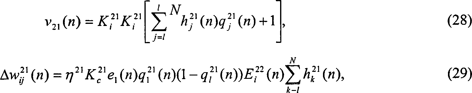
Δh12j (n) = η12K12i e2(n)q12i (n), (35) For compensator C ₁₂ :

q 12 1 (n) = φ (p 12 1 (N)). (32)

.delta.h 12 j (n) = η 12 K 12 i e 2 (N) q 12 i (n), (35)

In these equations, η ²¹ > 0 and η ¹² > 0 are the learning rate. K _c ²¹ > 0 and K _c ¹² > 0 are the respective controller gain for C ₂₁ and C _12, respectively. E _i ²¹ (n) is the delayed error signal of e ₁ (n), and E _i ¹² (n) is the delayed error signal of e ₂ (n).

The compensator sign factors K _s ²¹ and K _s ¹² 43 are a set of constants that relate to the types of action of the process as follows: K s 21 = 1, if G 22 and G 21 have different modes of action (36a) K s 21 = -1, if G 22 and G 21 have the same mode of action (36b) K s 12 = 1, if G 11 and G 12 have different modes of action (36d) K s 12 = -1, if G 11 and G 12 have the same mode of action (36d)

These Sign factors are required to ensure that the MFA compensators Generate signals in the right direction so that the disturbances, through the coupling factors of the multiply variable process caused, can be reduced.

Multi-variable processes can also be controlled by using single-loop MFA controllers. 6 shows a system diagram in which 2 model-free, adaptive controllers 62 with one loop each, to use a 2-input 2-output process 64 to control. In this case, the controllers will treat the coupling factors of the process as failures. This design has the advantage that the structure of the control system is simpler. Due to the powerful adaptive capability of the model-free adaptive controller, this system should work quite well for the multi-variable processes whose coupling factors are not very strong.

A 3 × 3 multi-variable, model-free, adaptive control system is available in 7 with a signal shown in the river plan. In the 3x3 MFA control system, the MFA controller set includes 66 three controllers C ₁₁ , C ₂₂ , C ₃₃ and six compensators C ₂₁ , C ₃₁ , C ₁₂ , C ₃₂ , C ₁₃ and C ₂₃ . The process 68 has nine subprocesses G ₁₁ to G ₃₃ . The process outputs as measured variables y ₁ , y ₂ and y ₃ are used as the feedback signals of the main control loops. They become at adders 70 is compared with the set values r ₁ , r ₂ and r ₃ to produce errors e ₁ , e ₂ and e ₃ . The output of each controller that one of the inputs e _1, e ₂ or e ₃ is associated, by adders 72 combined with the output of the compensators associated with the other two inputs to produce control signals u ₁ , u ₂ and u ₃ .

Without loss in generality Below is a set of equations that are arbitrary, multiple variable, model-free, adaptive N × N control system. Provided N = 3, it applies to the above-mentioned 3 × 3 MFA control system.

q111 (n) = φ(p11j (n)), (38)

Δh11j (n) = η11K11c e1(n)q11j (n), (41)wo l = 1, 2, ... N.For controller C _ll :

q 11 1 (n) = φ (p 11 j (n)), (38)

.delta.h 11 j (n) = η 11 K 11 c e 1 (N) q 11 j (n), (41) where l = 1, 2, ... N.

q lm / j(n) = φ(p lm / i(n)), (43)

Δhlmj (n) = ηlmKlmc em(n)qlmi (n) (46)wo l = 1, 2, ... N; m = 1, 2, ... N und l ≠ m.For compensator C _lm :

q lm / j (n) = φ (p lm / i (n)), (43)

.delta.h lm j (n) = η lm K lm c e m (N) q lm i (n) (46) where l = 1, 2, ... N; m = 1, 2, ... N and l ≠ m.

In these equations, η ^ll > 0 and η ^lm > 0 are the learning rate. K _c ^ll > 0 and K _c ^lm > 0 are the respective controller gain for C _ll and C _lm, respectively. E _i ^lm (n) is the delayed error signal of e ₁ (n), and E _i ^lm (n) is the delayed error signal of e _m (n).

K lm / S is the sign factor for the MFA compensator, which is chosen based on the effects of the subprocesses as follows: K S lm = 1, if G ll and G lm have different modes of action (47a) K S lm = -1, if G ll and G lm have the same mode of action (47b) where l = 1, 2, ... N; m = 1, 2, ... N; and l ≠ m.

C. Model-free, adaptive Control for Processes with big ones delays

In Process control applications have many processes having large time delays as a result of the delay in the transformation of heat, Materials and signals, etc. A good example is a tape rolling process, z. As a steel mill or a paper machine. It is completely the same which tax measures their effects are without a time delay period not measurable. If a PID is used in this case, the Controller output during the delay time constantly continue to grow and a big overshoot cause system reactions or even make the system unstable. Smith Predictor is a useful one Control scheme for coping of processes with big ones Time delays. However, designing a Smith Predictor is usually an exact process model is required because its performance otherwise could not be satisfactory.

8th FIG. 12 shows a block diagram for a model-free, adaptive, single-input, single-output, anti-delay control system including an MFA anti-delay controller 74 and a process with big time delays 76 , A special delay predictor has been designed to generate a dynamic signal y _c (t) to replace the measured variable y (t) as the feedback signal. The input to the controller 80 is then about adder 82 calculated as follows: e (t) = r (t) -y c (T). (48)

The Idea here is an e (t) signal for to generate the controller and let it "feel" its control effect without much delay, thus generating proper control signals will continue.

wo Y(S), Y_p(S), U(S) und Y_c(S) jeweils die Laplace-Transformationen von Signalen y(t), y_p(t), u(t) bzw. y_c(t) sind; wo y_p(t) das prädiktive Signal ist; wo y_c(t) der Ausgang des Prädiktors ist; wo K, T, τ die Parameter für den Prädiktor auf Basis des Prozessapproximationsmodells in einer FOLPD-Form sind. In echten Anwendungen kann DC-Gain K beim Geräteeichungs- und Datenkonvertierungsverfahren nahe 1 eingestellt werden. Der Benutzer kann die Prozessverzögerungszeit leicht grob abschätzen, die als τ im MFA-Prädiktor benutzt werden kann. T kann entweder vom Benutzer ausgewählt oder als 20T vorgegeben werden, wo T das Stichprobenintervall ist. Spätere Simulationen weisen auf, dass das MFA-Antiverzögerungssystem in Bezug auf diese Parameter nicht sehr empfindlich ist.Since the MFA controller of the system has a strong adaptive capability, the delay predictor can be designed in a simple form without knowing the quantitative information of the process. For example, it may be formed in a first-order generic lag-plus-delay (FOLPD) form, represented by the following Laplace transform function:

where Y (S), Y _p (S), U (S), and Y _c (S) each represent the Laplace transforms of signals y (t), y _p (t), u (t), and y _c (t ) are; where y _p (t) is the predictive signal; where y _c (t) is the output of the predictor; where K, T, τ are the parameters for the predictor based on the process approximation model in a FOLPD form. In real applications DC Gain K can be set close to 1 in the device calibration and data conversion process. The user can easily roughly estimate the process delay time, which can be used as τ in the MFA predictor. T can either be selected by the user or specified as 20T, where T is the sampling interval. Later simulations indicate that the MFA anti-delay system is not very sensitive to these parameters.

Compared with the traditional Smith Predictor is the process model for this Design is not required here, and the simulation shows it for processes with very big ones delays but still a big one control quality can achieve.

9 illustrates a 2x2 multi-variable, model-free, adaptive anti-delay control system. The MFA anti-delay controller set 84 includes two MFA controllers C ₁₁ and C ₂₂ , two compensators C ₂₁ and C ₁₂ and two predictors D ₁₁ and D ₂₂ . The process 86 has big time delays in the main control loops. Equation (49) can be used for the design of the predictor. A multi-variable MFA higher-order delay control system can be accordingly designed without loss of generality.

D. Model Free, Adaptive Cascade control system

If a process has two or more significant potential perturbations and the process can be split into two loops (one is fast and one is slow), then cascade control can be used to speed up perturbations and so on quality. As in 10 ₁ , a cascade system includes two controllers, the primary controller C ₁ and the secondary controller C ₂ . The inner loop 88 includes C ₂ and P ₂ , and the outer loop 92 includes C ₁ and P ₁ where P ₁ 90 consists of C ₂ , P ₂ and P ₃ . The output of C ₁ drives the setpoint of C ₂ .

Although Cascade control one of the most useful Control schemes is the process control, it is often found that the In real cascade control applications, the outer loop do not close. They usually do argue that the system reactions start to oscillate as soon as possible the outer loop is closed.

Because of the interacting nature of the control circuits in the cascade control system, it is far more important that controllers be properly tuned. However, if PI or PID controllers are used, 4 to 6 PID parameters must be tuned. It is not easy to find good combinations of such numerous parameters. If the process dynamics change frequently, the controllers need to be continually retuned because otherwise the interacting nature of the inner and outer loops can cause serious problems with system stability. Since the MFA controller is capable of well compensating for changes in the process dynamics, the closed-loop dynamics of the inner loop with MFA controller C ₂ does not show much change, even if the process dynamics of P ₂ u. U. changes greatly. This means that the interconnection of the outer and inner loop becomes much weaker. A more stable inner loop contributes to a more stable outer loop, and vice versa. Further, because each single-variable MFA controller has only one tuning parameter, the controller gain K _c , and it does not normally have to be tuned, it becomes much easier to start and maintain the model-free, adaptive cascade control system.

E. Simulation results

The results obtained by using the invention are best illustrated by the following simulation diagrams. The following notations are used in the discussion of these diagrams:
S - Laplace transform operator.
G _p (S) - Laplace transfer function of the process,
Y (S) - Laplace transform of y (t), the process output or the measured variable,
U (S) - Laplace transform of u (t), the process input or controller output.

The Relationship between Gp (S), Y (S) and U (S) is:

The Process models used in this simulation are in these equations shown:

11 and 12 show the simulation results of the MFA and PID control for a structure-variant process whose control is very difficult. In this case, process models 2 to 5 are used. The process models are brought online during the simulation to generate the structure change. In the simulation, the center position of the MFA controller gain K _c = 1, and PID is matched with K _p = 1, K _i = 10 and K _d = 2 on model 2. The overall controller tuning parameters remain unchanged, although the process is changing.

In 11 and 12 are the curves 100 and 106 Setpoints for MFA and PID, curves 104 and 110 are measured variables for MFA and PID, and curves 102 and 108 are the respective controller outputs for MFA or PID.

In 11 the process model starts with model 2 and then it changes to 3, just before the second set point change, approximately in the 4.5 minute position. In 12 the process model starts with model 4 and then changes to 5, just before the second setpoint change, approximately in the 3.7-minute range. It is readily apparent that the MFA controller can adapt very well to process structure changes while the PID controller is unable to do so.

13 to 15 show the simulation results of a 2 × 2 process, each controlled by a set of MIMO MFA controllers, two SISO MFA controllers and two SISO PID controllers. The 2 × 2 process is simulated on the basis of the process models 1, 2, 3 and 4 for P ₁₁ , P ₂₁ , P ₁₂ and P _22, respectively. This MIMO process is heavily coupled, making it rather difficult to control.

In 13 are curves 112 and 118 the setpoints r ₁ and r ₂ , curves 114 and 120 are the measured variables y ₁ and y ₂ , and curves 116 and 122 There are outputs v ₁₁ and v ₂₂ for MIMO MFA controllers C ₁₁ and C _22, respectively.

In 14 are curves 124 and 130 the setpoints r ₁ and r ₂ , curves 126 and 132 are the measured variables y ₁ and y ₂ , and curves 128 and 134 are outputs u ₁ and u ₂ for SISO MFA controllers C ₁ and C _2, respectively.

In 15 are curves 136 and 142 the setpoints r ₁ and r ₂ , curves 138 and 144 are the measured variables y ₁ and y ₂ , and curves 140 and 146 are outputs u ₁ and u ₂ for SISO PID controllers C ₁ and C _2, respectively.

When comparing 13 . 14 and 15 It should be noted that the MIMO MFA has the best control quality and the SISO PID the worst control performance. Without the compensators, the output u _{2 of} the SISO controller C ₂ drops to 0 percent, limited by the lower limit. With the MIMO MFA compensators, the MIMO controller achieves a wider operating range so that its output v ₂₂ can remain within the working range. In addition, the other control loop is affected by the disturbances caused by the setpoint changes on a much smaller scale. Finally, the MIMO-MFA control can increase the control performance of the system and its stability range. In these simulations, the K _{c of} the MFA controllers are set as the default setting without tuning to 1. The PID controller is well tuned, but its performance is still not very satisfactory.

16 and 17 Figure 4 shows the simulation results of a process controlled by an MFA delay controller with other delay predictor parameters. model 6 is used to simulate a process with large time delays. In these pictures show curves 148 and 158 the setpoint r (t), curves 150 and 160 show the real measured variable y (t), curves 152 and 162 show the controller output u (t), curves 154 and 164 show the output of the predictor y _c (t), and curves 156 and 166 show the predictive signal y _p (t).

Ein PID-Controller kann normalerweise einen Prozess mit einem Verhältnis zwischen τ und T von etwa 1 bewältigen. Hier bei Modell 6 ist dieses Verhältnis zwischen τ und T so hoch wie 9. (τ = 90, dominante Zeitkonstante T = 10). Das zu bewältigen, ist für jede Art normaler Controller sehr schwierig. Der MFA-Antiverzögerungs-Controller kann diesen Prozess jedoch ganz leicht steuern. In 16 ist Prädiktor τ = 90, T = 20, was ziemlich gut mit dem Prozess übereinstimmt. In 17 wird vorsätzlich eine Fehlanpassung zwischen Prädiktorparametern und Prozess erzeugt. Die Prädiktorparameter sind τ = 75, T = 20, die Prozessparamenter sind τ = 90, Dominante T = 10. Ihre Fehlanpassung ist signifikant. Entsprechend 17 kann der MFA den Prozess aber immer noch gut steuern. Der MFA-Antiverzögerungs-Controller bietet wesentliche Vorteile im Vergleich zum traditionellen Smith-Predictor-Steuerschema.The effect of the time delay on the process dynamics is related to the time constant. Normally, the ratio between τ and T is used to measure the significance of time delay effects on a process, as follows:

A PID controller can normally handle a process with a ratio between τ and T of about one. Here in model 6, this ratio between τ and T is as high as 9 (τ = 90, dominant time constant T = 10). This is very difficult for any kind of normal controller. The MFA antivirals However, the controller can easily control this process. In 16 is a predictor τ = 90, T = 20, which agrees pretty well with the process. In 17 A mismatch between predictor parameters and process is intentionally generated. The predictor parameters are τ = 75, T = 20, the process parameters are τ = 90, dominant T = 10. Their mismatch is significant. Corresponding 17 but the MFA can still control the process well. The MFA anti-delay controller offers significant advantages over the traditional Smith Predictor control scheme.

18 shows the simulation results related to the control of processes with large time delays with normal MFA and PID controllers. In 18 are curves 168 and 174 the setpoints, curves 170 and 176 are the measured variables, and curves 172 and 178 are the outputs. The process model 7 is used for the simulation. Since the τ / T ratio for model 7 (τ = 20, dominant T = 10) is 2, it is much easier to control than model 6. However, it can be seen that even a MFA can not control this process very well, while a PID can not handle a process of this kind at all, no matter how you tune it. This simulation also implies the value of the MFA anti-delay controller included in 16 and 17 is shown.

19 and 20 show the MFA and PID control for cascade systems.

In 19 are curves 180 and 186 Setpoints for C ₁ and C ₂ , curves 182 and 188 are measured variables for C ₁ and C ₂ , and curves 184 and 190 are each outputs for C ₁ or C ₂ .

In 20 are curves 192 and 198 Setpoints for C ₁ and C ₂ , curves 194 and 200 are measured variables for C ₁ and C ₂ , and curves 196 and 202 are each outputs for C ₁ or C ₂ .

The simulation starts when both the inner loop and the outer loop are open and u ₂ (curve 190 or 202 ) is set to 20 percent. The inner loop is closed by turning the auto / manual switch of C ₂ at the 3 minute position to automatic and its setpoint r ₂ (curve 186 or 198 ) is increased from 20 to 30 percent. It can be seen that the inner loop can be well controlled by both the MFA and the PID. The remote / local switch of C ₂ is set to remote and requests a remote setpoint at the 4.8 minute position. It will set the setpoint of C ₂ , r ₂ (curve 186 or 198 ) force the output of C ₁ , u ₁ (curves 184 . 196 ) to follow. Thereafter, the outer loop is closed by turning the auto / manual switch from C ₁ to Auto. Then both control loops are closed and the system is cascaded. The control quality of the cascade system is changed by changing the setpoint value of C ₁ , r ₁ (curve 180 or 192 ) simulates. It can be seen that the MFA controllers can control the cascade system without any special requirements. The controller gain K _c = 1 is the default setting for both MFA C ₁ and C ₂ . On the other hand, the PID-controlled system quickly becomes unstable. During this simulation, every effort was made to match the PID, but the result was unsatisfactory. The reason is the sensitivity of PID to changes in process dynamics. In fact, interactions between the inner and outer circuits of a cascade system produce significant dynamic changes.

F. Simulation of the real process

wo X_D die höchste Komposition oder Destillationskomposition ist, X_B die unterste Komposition ist, R_f die Rücklaufströmung ist, S_f die Dampfströmung ist und F_r die Zuführgeschwindigkeit ist. D₁₁ und D₂₂ sind die Störungen, die durch die Änderung der Zuführgeschwindigkeit verursacht werden.For the simulation of the MIMO-MFA control system, a real model of a distillation column, the Wood and Berry Column 21, is selected. The model is represented by the following Laplace transfer functions:

where X _{D is} the highest composition or distillation composition, X _{B is} the lowest composition, R _{f is} the return flow, S _{f is} the vapor flow, and F _{r is} the feed rate. D ₁₁ and D ₂₂ are the disturbances caused by the change of the feeding speed.

21 and 22 show the simulation results for this distillation column with a 2x2 MFA controller set. 21 shows the control quality for setpoint changes, and 22 shows the control quality for load changes.

In 21 are curves 204 and 210 the setpoints for C ₁₁ and C ₂₂ , curves 206 and 212 are the measured variables for C ₁₁ and C ₂₂ , and curves 208 and 214 are the respective outputs for C ₁₁ and C _22, respectively. It can be seen that r ₁ (curve 204 ) is increased at the 1.3 minute position and r ₂ (curve 210 ) is reduced approximately at the 4-minute and 6-minute intervals. This demonstrates good overall control performance. Due to the functions of the MFA compensators included in the MIMO MFA controller set, the disturbances are small in size. If normal PID controllers were used, the disturbances would be far more significant, which would cause significant control problems.

In 22 are curves 216 and 222 the setpoints for C ₁₁ and C ₂₂ , curves 218 and 224 are the measured variables for C ₁₁ and C ₂₂ , and curves 220 and 226 are the respective outputs for C ₁₁ and C _22, respectively. Curve 228 is the feed rate setpoint f _r (t) (F _r (S) in Laplace transform), and curves 230 and 232 are the spurious signals d ₁₁ (t) and d ₂₂ (t) (D ₁₁ (S) and D ₂₂ (S) in Laplace transform) caused by the feed speed change. The simulation shows that the feed rate changes twice at the 2-minute and 3.3-minute intervals, which disturbs the system. The MFA controllers can compensate for these disturbances.

Claims (22)

Model-free adaptive control system for a stable, controllable and direct acting or to reverse-acting industrial open-loop process ( 12 ) with a process input (u (t)), a process output (x (t)) that is a component of a measured process variable (y (t)), a sensitivity function that satisfies the ratio ∂y (t) / ∂u (t ) between the partial derivatives with respect to time of said process output (x (t)) and said process input (u (t)), and a control target function E _s (t) calculated from the error value (e (t)) being the difference between a measured process variable (y (t)) and a selected setpoint (r (t)), characterized in that the system comprises: a) a dynamic block having an error input (e (t)) and a control value output (v (t)), wherein said dynamic block is arranged to iteratively vary over a moving time window said control value output (v (t)) to minimize said error value (e (t)) ; and b) a learning mechanism for continuously iteratively modifying the parameters of said dynamic block to vary said control value output (v (t)) to reduce said error value (e (t)); c) wherein said process is directed according to the control value output (v (t)) used as process input (u (t)). The system of claim 1, further characterized that said learning mechanism only measured on the said Process variable (y (t)), the said control value (v (t)) and the setpoint (r (t)) based. A system according to claim 1 or 2, further characterized in that an arbitrary nonzero constant for the actual sensitivity function of said process ( 12 ) is substituted in said learning mechanism. System according to claim 3, characterized in that the said arbitrary Constant is 1. A system according to any one of claims 1 to 4, characterized in that said control objective function E _{s (t)} = _{1 /} 2e (t) ² and e (t) is said difference value between said measured process variable (y (t)) and the said setpoint value (r (t)) is. System according to one of claims 1 to 5, characterized in that said dynamic block is a neural network ( 18 ) as direct inputs ( 20 ) has a plurality of successive time delayed inputs (E ₁ to E _N ) of said error value (e (t)). System according to one of Claims 1 to 6, characterized in that the output (o (t)) of said neural network ( 18 ) and said error value (e (t)) for generating said control value (v (t)) are added. System according to one of claims 1 to 7, adapted to a process ( 76 ), in which the measured process variable (y (t)) has a large time delay in responding to said process input (u (t)), characterized in that it further comprises: a) a delay predictor ( 78 ) whose inputs are said measured process variable (y (t)) and said process input (u (t)), the output of said delay predictor being:

where Y (S), U (S) and Y _c (S) respectively represent the Laplace transforms of said measured variables (y (t)), said process input (u (t)) and said delay predictor output (y _c (t )) are; K, T and τ are constants; and b) the error value (e (t)) is calculated by e (t) = r (t) -y _c (t). System according to claim 8, characterized in that K is essentially 1 and T and τ are chosen to be known Response delay parameters approaching the said process. System according to one of Claims 1 to 9, characterized in that a) said dynamic block is a three-layer artificial neural network ( 18 ) comprising: i) a first layer ( 20 ) of a first plurality of neurons each having as input and output (E ₁ to E _N ) a value representative of said error value (e (t)) in one of the plurality of successive iterations; ii) a second layer ( 22 ) from a second plurality of neurons ( 30 each having as inputs the outputs of each of said first plurality of neurons multiplied by a first variable weighting factor (w _ij ) and whose output value (p ₁ to p _N ) is the sum of their input values; and iii) a third-layer neuron whose inputs (q ₁ to q _N ) are values corresponding to the output value (p ₁ to p _N ) of each of said second plurality of neurons multiplied by a second variable weighting factor (h _j ), and whose output value is the sum of its input values; b) said control value (v (t)) being a value representative of the sum of the neural network output (o (t)) and said error value (e (t)) in the current iteration; c) wherein said first weighting factor (w _ij ) is updated continuously in successive iterations according to the following formula:

where Δw _{ij is} the change in the weighting factor of the output of the i-th first plurality neuron to the j-th second plurality neuron from the last previous iteration to the current iteration; η is a preselected learning factor; K _{c is} a preselected constant; ∂y (t) / ∂u (t) is the sensitivity function of said process; e is the error value; q _{j is} the normalized output of the j-th second plurality neuron; E _{i is} the normalized error value applied to the ith first-plurality neuron; N is the number of first plurality neurons; Σh _{k is} the sum of said second weighting factors; and (n) denotes the current iteration; and d) wherein said second weighting factor (h _j ) is continuously updated in successive iterations according to the following formula

where Δh _{j is} the change in the weighting factor of the output of the j-th second plurality neuron to said third-layer neuron from the last previous iteration to the current iteration. Model-free adaptive control system for a plurality of stable interacting industrial open-loop processes ( 46 . 54 or 68 ) each with a process input (u ₁ , u ₂ , ...), a measured process output (x ₁₁ , x ₂₁ , x ₁₂ , x ₂₂ , ...), a sensitivity function that relates the relationship between the partial derivatives with respect at the time of said process output and said process input; and a control target function E _s (t) calculated from the error values (e ₁ , e ₂ , ...), each representing the difference between the measured process variable (y ₁ , y ₂ , ...) of a corresponding process and a selected setpoint (r ₁ , r ₂ , ...) for this process; characterized in that said system comprises: a) a first plurality of controllers (C ₁₁ , C ₂₂ , ...) each having an error value input (e ₁ , e ₂ , ...) and a control value output (v ₁₁ , v ₂₂ , ...); and a second plurality of compensators (C ₂₁ , C ₁₂ , ...) each having an error value input (e ₁ , e ₂ , ...) and a compensation value output (v ₂₁ , v ₁₂ , ...); b) a plurality of adders ( 58 or 72 ) with the task for each of said control value outputs (v ₁₁ , v ₂₂ , ...) of said controller (C ₁₁ , C ₂₂ , ...), the compensation value outputs (v ₂₁ , v ₁₂ , ...) of said To add compensators (C ₂₁ , C ₁₂ , ...); c) the output of each said adder being used as process input (u ₁ , u ₂ , ...) from one of said interacting processes (G ₁₁ , G ₂₁ , G ₁₂ , G ₂₂ , ...); and d) a learning mechanism for continuously iteratively modifying the parameters of each of said controllers and compensators to vary said control values (v ₁₁ , v ₂₂ , ...) and compensation values (v ₂₁ , v ₁₂ , ...) by said To reduce error values (e ₁ , e ₂ , ...); wherein said learning mechanism is based only on said measured process variables (y ₁ , y ₂ , ...), control values (v ₁₁ , v ₂₂ , ...) and said set values (r ₁ , r ₂ , ...) , System according to claim 11, characterized in that that said learning mechanism iteratively the said parameters dependent on modified by the aforementioned sensitivity functions in which arbitrary Non-zero constants for the actual Sensitivity functions of said processes are substituted. System according to claim 12, characterized in that that said arbitrary Constant is 1. A system according to claims 11 to 13, characterized in that said control objective function is E _{s (t)} = _1/2 e (t) ² , where e (t) represents each of the error values (e ₁ (t), e ₂ (t) , ...) representing the difference values between the said measured process variables (y ₁ , y ₂ , ...) and said setpoints (r ₁ , r ₂ , ...) are. A system according to claims 11 to 14, characterized in that said controllers (C ₁₁ , C ₂₂ , ...) and compensators (C ₂₁ , C ₁₂ , ...) are artificial neural networks. System according to Claim 15, characterized in that a) each said controller (C ₁₁ , C ₂₂ , ...) and compensator (C ₂₁ , C ₁₂ , ...) is a three-layer artificial neural network ( 18 ), which in turn comprises: i) a first layer ( 20 ) of a first plurality of neurons each having as inputs and outputs (E ₁ to E _N ) a value corresponding to said error value (e ₁ , e ₂ , ...) in one of a plurality of successive iterations is representative; ii) a second layer ( 22 ) from a second plurality of neurons ( 30 each having as inputs the values of the outputs of each of said first plurality of neurons multiplied by a first variable weighting factor (w _ij ); and whose output value (p ₁ to p _N ) is the sum of their input values; and iii) a third-layer neuron ( 34 ) whose inputs (q ₁ to q _N ) are values representative of the output value (p ₁ to p _N ) of each of said second plurality of neurons multiplied by a second variable weighting factor (h _j ) and whose output value is the sum of its Input values is; b) each of said control values (v ₁₁ , v ₂₂ , ...) being a value corresponding to the sum of the neural network output (o (t)) and said error value (e ₁ , e ₂ , ... ) is representative in the current iteration; c) wherein said first weighting factor is continuously updated in each said controller in successive iterations according to the following formula:

and in each said compensator according to the following formula:

where Δw _{ij is} the change in the weighting factor of the output of the i-th first plurality neuron to the j-th second plurality neuron from the last previous iteration to the current iteration; η is a preselected learning factor; K _{c is} a preselected positive controller gain replacing the sensitivity function ∂y (t) / ∂u (t) of said process; e is the error value for a particular controller or compensator; q _{j is} the normalized output of the j-th second plurality neuron; E _{i is} the normalized delayed error value applied to the ith first-plurality neurons of this controller or compensator; Σh _{k is} the sum of said second weighting factors; (n) denotes the current iteration; N is said first plurality; and l and m = 1, 2, ... N with l ≠ m; and d) wherein said second weighting factor is continuously updated in successive iterations in each said controller according to the following formula: .delta.h ll j (n) = η ll K ll c e 1 (N) q ll j (N) and in each of said compensators according to the following formula: .delta.h lm j (n) = η lm K lm c e m (N) q lm j (N) where Δh _{j is} the change of the weighting factor of the output of the jth second plurality neuron to said third layer neuron from the last previous iteration to the current iteration. A system according to claim 16, characterized in that the output of controller II is as follows:

and the output of the compensator lm is as follows:

where K _s ^{lm is} a sign factor which is 1 if processes ll and lm are of different acting types, and -1 if processes ll and lm are of the same acting type. System according to one of claims 11 to 17, adapted to processes ( 86 ) in which the measured process variables (y ₁ , y ₂ , ...) have a large time delay in response to said process inputs (u ₁ , u ₂ , ...), characterized in that it further comprises: a) delay predictors (D ₁₁ , D ₂₂ ,...) having as inputs said measured process variables (y ₁ , y ₂ , ...) and said process inputs (u ₁ , u ₂ , ...), the outputs of said delay predictors are as follows:

where Y (S), U (S) and Y _c (S) are the Laplace transforms of each of said measured process variables (y ₁ , y ₂ , ...), the process inputs (u ₁ , u ₂ , ...) and the delay _{predictor outputs} (y _c1 , y _c2 , ...); K, T and τ are constants, and b) the error values (e ₁ , e ₂ , ...) are calculated by e ₁ (t) = r ₁ (t) - y _c1 (t), e ₂ (t) = r ₂ (t) - y _c2 (t), ... Model-free adaptive cascade control system for stable, controllable and direct-acting or reverse-acting industrial open-loop processes consisting of a plurality of serially connected sub-processes (P ₂ and P ₃ ) with different control requirements, each process having a sub-process input, a sub-process output, the sub-process input of the next subprocess in the series, and has a sensitivity function which is the ratio between the partial derivatives with respect to time of said process output and said process input, said system comprising means for measuring the output (y ₁ ) of the last subprocess ( P ₃ ) in said series and being characterized by comprising: a) a plurality of serially connected controllers (C ₁ and C ₂ ) each having an error value input (e ₁ or e ₂ ), the input (e ₁ ) of the first controller (C ₁ ) the difference between the measured output ( y ₁ ) of the last subprocess (P ₃ ) and a selected desired value (r ₁ ), and the input (e ₂ ) of the second controller (C ₂ ) is the difference between the measured output (y ₂ ) of the first subprocess (P ₂ ) and the output (u ₁₎ of the first controller (C _1), each controller a control value output (u _1, u has ₂₎ and is designed such that it iteratively varied over a moving time window of the control value mentioned, to minimize said error values (e ₁ , e ₂ ); b) where a control objective function is E _{s (t)} = ½e (t) ² , where e (t) represents the error values (e ₁ (t), e ₂ (t)) representing the difference values between said measured process variables ( y ₁ , y ₂ ) and said setpoints (r ₁ , r ₂ ); c) a learning mechanism with the task of continuously iteratively modifying the parameters for said controllers to vary said controller outputs (u ₁ , u ₂ ) to reduce all said error values (e ₁ , e ₂ ), said learning mechanism only based on said measured process outputs (y ₁ , y ₂ ), said controller outputs (u ₁ , u ₂ ) and said setpoint (r1, r2). The system of claim 19, further characterized that an arbitrary Nonzero constant for the actual Sensitivity function of each of the mentioned subprocesses in the substituted learning mechanism is substituted. Method for controlling a system with a variable Entrance, an exit and an unknown relationship between the said input and said output, without approximation or Modeling of said relationship, characterized in that the method comprises the following steps: a) Select one Setpoint representing a setpoint of said output; b) Calculate an error value that depends on the difference between the said setpoint and said output is dependent; c) Apply of said error value to a controller that has a dynamic Contains block its only inputs delayed Functions of the mentioned error value are and whose output Is part of a control value that varies the said factory input; and d) continuous iterative variation of the parameters of said dynamic block, only by said error value to minimize. The method of claim 21, further characterized in that the method includes the step of adding said error value to said dynamic block output to obtain the ge to generate the control value.