CN112149794A - Information processing apparatus, computer-readable storage medium, and information processing method - Google Patents
Information processing apparatus, computer-readable storage medium, and information processing method Download PDFInfo
- Publication number
- CN112149794A CN112149794A CN202010466951.3A CN202010466951A CN112149794A CN 112149794 A CN112149794 A CN 112149794A CN 202010466951 A CN202010466951 A CN 202010466951A CN 112149794 A CN112149794 A CN 112149794A
- Authority
- CN
- China
- Prior art keywords
- matrix
- matrices
- calculation
- stored
- elements
- Prior art date
- Legal status (The legal status is an assumption and is not a legal conclusion. Google has not performed a legal analysis and makes no representation as to the accuracy of the status listed.)
- Pending
Links
- 238000003860 storage Methods 0.000 title claims abstract description 63
- 230000010365 information processing Effects 0.000 title claims abstract description 42
- 238000003672 processing method Methods 0.000 title claims abstract description 10
- 239000011159 matrix material Substances 0.000 claims abstract description 328
- 238000004364 calculation method Methods 0.000 claims abstract description 152
- 238000000034 method Methods 0.000 claims abstract description 74
- 238000004422 calculation algorithm Methods 0.000 claims abstract description 46
- 230000008569 process Effects 0.000 claims abstract description 32
- 238000012545 processing Methods 0.000 claims description 43
- 230000006870 function Effects 0.000 claims description 35
- 238000013135 deep learning Methods 0.000 claims description 21
- 239000006185 dispersion Substances 0.000 claims description 8
- 230000014509 gene expression Effects 0.000 description 59
- 238000010586 diagram Methods 0.000 description 41
- 238000003491 array Methods 0.000 description 16
- 238000010606 normalization Methods 0.000 description 14
- 239000013598 vector Substances 0.000 description 12
- 238000013528 artificial neural network Methods 0.000 description 11
- 210000004027 cell Anatomy 0.000 description 5
- PTNZGHXUZDHMIQ-CVHRZJFOSA-N (4s,4ar,5s,5ar,6r,12ar)-4-(dimethylamino)-1,5,10,11,12a-pentahydroxy-6-methyl-3,12-dioxo-4a,5,5a,6-tetrahydro-4h-tetracene-2-carboxamide;hydrochloride Chemical compound Cl.C1=CC=C2[C@H](C)[C@@H]([C@H](O)[C@@H]3[C@](C(O)=C(C(N)=O)C(=O)[C@H]3N(C)C)(O)C3=O)C3=C(O)C2=C1O PTNZGHXUZDHMIQ-CVHRZJFOSA-N 0.000 description 3
- 101150108288 DPE1 gene Proteins 0.000 description 3
- 239000000872 buffer Substances 0.000 description 3
- 238000013527 convolutional neural network Methods 0.000 description 3
- 238000005070 sampling Methods 0.000 description 3
- 238000013459 approach Methods 0.000 description 2
- 230000006872 improvement Effects 0.000 description 2
- 238000003909 pattern recognition Methods 0.000 description 2
- 230000001174 ascending effect Effects 0.000 description 1
- 210000004556 brain Anatomy 0.000 description 1
- 230000008859 change Effects 0.000 description 1
- 238000009826 distribution Methods 0.000 description 1
- 230000007786 learning performance Effects 0.000 description 1
- 239000004973 liquid crystal related substance Substances 0.000 description 1
- 238000010801 machine learning Methods 0.000 description 1
- 238000004519 manufacturing process Methods 0.000 description 1
- 230000003278 mimic effect Effects 0.000 description 1
- 238000012986 modification Methods 0.000 description 1
- 230000004048 modification Effects 0.000 description 1
- 210000002569 neuron Anatomy 0.000 description 1
- 238000005192 partition Methods 0.000 description 1
- 238000011176 pooling Methods 0.000 description 1
- 230000000644 propagated effect Effects 0.000 description 1
- 238000011160 research Methods 0.000 description 1
- 239000004065 semiconductor Substances 0.000 description 1
- 239000007787 solid Substances 0.000 description 1
Images


Classifications
-
- G—PHYSICS
- G06—COMPUTING; CALCULATING OR COUNTING
- G06F—ELECTRIC DIGITAL DATA PROCESSING
- G06F17/00—Digital computing or data processing equipment or methods, specially adapted for specific functions
- G06F17/10—Complex mathematical operations
- G06F17/15—Correlation function computation including computation of convolution operations
- G06F17/153—Multidimensional correlation or convolution
-
- G—PHYSICS
- G06—COMPUTING; CALCULATING OR COUNTING
- G06F—ELECTRIC DIGITAL DATA PROCESSING
- G06F17/00—Digital computing or data processing equipment or methods, specially adapted for specific functions
- G06F17/10—Complex mathematical operations
- G06F17/16—Matrix or vector computation, e.g. matrix-matrix or matrix-vector multiplication, matrix factorization
-
- G—PHYSICS
- G06—COMPUTING; CALCULATING OR COUNTING
- G06N—COMPUTING ARRANGEMENTS BASED ON SPECIFIC COMPUTATIONAL MODELS
- G06N3/00—Computing arrangements based on biological models
- G06N3/02—Neural networks
- G06N3/04—Architecture, e.g. interconnection topology
- G06N3/045—Combinations of networks
-
- G—PHYSICS
- G06—COMPUTING; CALCULATING OR COUNTING
- G06N—COMPUTING ARRANGEMENTS BASED ON SPECIFIC COMPUTATIONAL MODELS
- G06N3/00—Computing arrangements based on biological models
- G06N3/02—Neural networks
- G06N3/06—Physical realisation, i.e. hardware implementation of neural networks, neurons or parts of neurons
- G06N3/063—Physical realisation, i.e. hardware implementation of neural networks, neurons or parts of neurons using electronic means
-
- G—PHYSICS
- G06—COMPUTING; CALCULATING OR COUNTING
- G06N—COMPUTING ARRANGEMENTS BASED ON SPECIFIC COMPUTATIONAL MODELS
- G06N3/00—Computing arrangements based on biological models
- G06N3/02—Neural networks
- G06N3/08—Learning methods
-
- G—PHYSICS
- G06—COMPUTING; CALCULATING OR COUNTING
- G06N—COMPUTING ARRANGEMENTS BASED ON SPECIFIC COMPUTATIONAL MODELS
- G06N3/00—Computing arrangements based on biological models
- G06N3/02—Neural networks
- G06N3/08—Learning methods
- G06N3/084—Backpropagation, e.g. using gradient descent
Abstract
The invention relates to an information processing apparatus, a computer-readable storage medium, and an information processing method. The information processing apparatus includes: a calculation unit that calculates a combination of t and q that minimizes a calculation time when q calculation cores calculate convolutions between a plurality of first matrices and a plurality of second matrices of t rows and t columns in parallel using a Winograd algorithm, a total number of elements of the plurality of first matrices and the plurality of second matrices not exceeding a number of data sets that can be stored in each of q storage areas of a register, the q calculation cores corresponding to the q storage areas, respectively; an output unit that outputs a program for causing a computing machine to execute a process, the process including: storing the plurality of first matrices and the plurality of second matrices in respective ones of the q storage areas using a combination of t and q; a convolution between the first matrix and the second matrix is computed by each of q computation kernels using a Winograd algorithm, the computation machine comprising q computation kernels and registers.
Description
Technical Field
Certain aspects of embodiments described herein relate to an information processing apparatus, a non-transitory computer-readable storage medium, and an information processing method.
Background
Machine learning using a multilayer neural network is called deep learning, and is applied to various fields. Various calculations are performed in each layer of the deep learning. For example, in the convolutional layer, convolution between image data and a filter is performed, and the result thereof is output to the subsequent layer. Since convolution is an operation between matrices, the amount of calculation thereof is large, resulting in a delay in the processing speed of learning. Therefore, Winograd algorithm is proposed as an algorithm for reducing the amount of convolution calculation. Note that techniques related to the present disclosure are also disclosed in the following documents: "Fast Algorithms for volumetric Neural Networks", Andrew Lavin et al, IEEE Computer Vision and Pattern Recognition (CVPR) conference, 2016, pages 4013 to 4021; and "Deep research Learning for Image Recognition", Kaiming He et al, IEEE Computer Vision and Pattern Recognition (CVPR) conference, 2016, pages 770 to 778.
However, the Winograd algorithm has room for improvement in terms of further increasing the processing speed of convolution.
Disclosure of Invention
The present invention has been made in view of these circumstances, and an object of the present invention is to improve the calculation speed of convolution.
According to an aspect of an embodiment, there is provided an information processing apparatus including: a calculation unit for calculating a combination of t and q that minimizes a calculation time when q calculation cores calculate convolutions between a plurality of first matrices and a plurality of second matrices of t rows and t columns in parallel using a Winograd algorithm, wherein a total number of elements of the plurality of first matrices and the plurality of second matrices does not exceed a number of data sets that can be stored in each of q storage regions of a register, and the q calculation cores correspond to the q storage regions, respectively; and an output unit for outputting a program for causing a computing machine to execute a process, the process including: storing the plurality of first matrices and the plurality of second matrices in respective ones of q storage areas using the calculated combinations of t and q, and calculating a convolution between the first matrices and the second matrices using a Winograd algorithm by each of q calculation cores, the calculation machine including q calculation cores and a register.
Drawings
Fig. 1 schematically shows a process flow of deep learning;
FIG. 2 schematically illustrates convolution performed in a convolutional layer;
3A-3C schematically illustrate convolution between a bottom matrix and a weight matrix;
fig. 4A to 4C schematically show the Winograd algorithm in the forward process;
FIG. 5 is a hardware configuration diagram of a computing machine for performing convolution in deep learning;
FIG. 6A is a hardware configuration diagram of a chain of DPUs, and FIG. 6B is a hardware configuration diagram of a DPU;
FIG. 7 is a hardware configuration diagram for each DPE;
fig. 8 is a hardware configuration diagram of DPE 0;
fig. 9 is a diagram for describing row numbers assigned to the banks R # 0 to R # 7;
fig. 10A to 10C are (first) schematic diagrams for describing a sequential method;
fig. 11A to 11C are (second) schematic diagrams for describing a sequential method;
fig. 12 is a schematic diagram for describing a multicast method;
FIG. 13 schematically shows the contents of register G # 0 of each DPE;
FIG. 14 schematically illustrates array elements of array g in main memory;
fig. 15 shows the contents of register G # 0 of DPE0 immediately after the array element is transmitted by the multicast method;
FIG. 16 shows the contents of register G # 0 of DPE0 after sorting;
FIG. 17 shows the contents of register G # 0 of DPE0 through DPE7 after sorting;
FIG. 18 is a schematic diagram of bank R # 0 of register G # 0 of DPE 0;
fig. 19 is a hardware configuration diagram of an information processing apparatus according to an embodiment;
fig. 20 is a functional configuration diagram of an information processing apparatus according to an embodiment;
FIG. 21 is a functional block diagram of a computing machine;
fig. 22 illustrates contents of registers G # 0 of the DPEs 0 through 7 in which arrays d and G are stored by a storage unit when forward processing is performed in the embodiment;
fig. 23A and 23B are (first) diagrams showing the contents of registers G # 0 to G # 3 of the DPE0 when the calculation unit performs convolution using the Winograd algorithm in the embodiment;
fig. 24 is a (second) diagram showing the contents of registers G # 0 to G # 3 of the DPE0 when the calculation unit performs convolution using the Winograd algorithm in the embodiment;
fig. 25 is a (third) diagram showing the contents of registers G # 0 to G # 3 of the DPE0 when the calculation unit performs convolution using the Winograd algorithm in the embodiment;
FIG. 26 is a diagram showing the calculation of equation (19) of an embodiment in order of steps;
fig. 27 is a diagram showing calculation of equation (21) of the embodiment in order of steps;
fig. 28 is a flowchart of an information processing method according to an embodiment;
fig. 29A to 29C are diagrams when convolution between a top matrix and a weight matrix is performed using a Winograd algorithm in a backward process according to an embodiment;
FIG. 30 shows the contents of register G # 0 of DPE0 through DPE7 where arrays y and G are stored by memory cells according to an embodiment;
31A and 31B are schematic diagrams of a convolution between a top matrix and a bottom matrix performed using Winograd's algorithm in a backward process according to an embodiment;
fig. 32A to 32C are schematic diagrams of convolution between a top matrix and a bottom matrix performed using the Winograd algorithm in a backward process according to an embodiment;
FIG. 33 is a diagram illustrating the contents of register G # 0 of DPE0 through DPE7 where arrays y and d are stored by memory cells according to an embodiment;
fig. 34 shows the contents of register G # 0 of DPE0 in which arrays d and G are stored by the storage unit when performing 1 × 1 convolution in an embodiment;
FIG. 35 shows contents of register G # 0 of DPE0 where a sub-base matrix d is stored by a storage unit during batch normalization according to an embodiment; and
fig. 36A and 36B show the contents of the register G # 0 of the DPE0, and are diagrams for describing the calculation performed by the calculation unit according to the embodiment during batch normalization.
Detailed Description
Before describing the embodiments, the projects studied by the inventors will be described.
Fig. 1 schematically shows a process flow of deep learning. In the deep learning, the neural network learns the feature of the recognition target by supervised learning of the recognition target such as an image. Using the neural network after learning enables the recognition target to be recognized.
Neural networks are networks in which the elements of neurons that mimic the brain are hierarchically connected. Each unit receives data from another unit and transmits data to yet another unit. In the neural network, various recognition targets can be recognized by changing parameters of the cells through learning.
Hereinafter, referring to fig. 1, a Convolutional Neural Network (CNN) for recognition of an image will be described.
The neural network has a multi-layer structure including convolutional layers, sub-sampling layers, and fully-connected layers. In the example of fig. 1, two convolutional layers and two sub-sampling layers are alternately arranged, but three or more convolutional layers and three or more sub-sampling layers may be provided. Furthermore, a plurality of fully connected layers may be provided. The multilayer structure of the neural network and the configuration of each layer may be predetermined by a designer according to an object to be identified.
The process of identifying images by neural networks is also referred to as forward processing. In the forward process, the convolutional and pooling layers are repeated alternately from left to right as shown in FIG. 1. Then, finally, the recognition target included in the image is recognized in the full connection layer.
Further, the process of learning an image through a neural network is also referred to as a backward process. In the backward processing, an error between the recognition result and the correct answer is obtained, and the obtained error is propagated from right to left backward through the neural network to change parameters of each layer of the convolutional neural network.
Fig. 2 schematically shows a convolution performed in a convolutional layer.
Fig. 2 shows a convolution between a bottom matrix in which pixel data of an input image is stored in each element and a weight matrix representing a filter acting on the input image. In this example, a plurality of bottom matrices and a plurality of weight matrices are prepared, and convolution between them is performed.
Each bottom matrix is identified by a lot number N and an input channel number Cin. On the other hand, each weight matrix is identified by an output lane number Cout and an input lane number Cin.
In the example of fig. 2, the convolution is performed as follows. First, a combination of lot number N and output channel number Cout is selected. For example, N ═ 0 and Cout ═ 0.
Then, from among combinations of a plurality of bottom matrices having the selected lot number N and a plurality of weight matrices having the selected output lane number Cout, a combination of a bottom matrix having the same input lane number Cin and a weight matrix is selected. For example, when N is 0 and Cout is 0 as described above, a base matrix in which N is 0 and Cin is 0 and a weight matrix in which Cout is 0 and Cin is 0 are selected.
Then, a convolution between the selected bottom matrix and the selected weight matrix is performed. Hereinafter, the matrix obtained by this convolution is referred to as a top matrix.
By performing such convolution between the bottom matrix of Cin ═ 0 to 255 and the weight matrix with the lot number N and the output channel number Cout fixed, 256 top matrices are obtained. Thereafter, by adding these 256 top matrices, one output matrix identified by the lot number N and the output channel number Cout is obtained.
Further, by performing the above calculation while changing the lot number N and the output channel number Cout, an output matrix of the total number of lot numbers N × the total number of output channel numbers Cout is obtained. In the example of fig. 2, 64 × 384 output matrices are obtained.
In the foregoing manner, convolution between the plurality of bottom matrices and the plurality of weight matrices is performed.
As described above, in such convolution, the convolution between the base matrix and the weight matrix having the same input channel number Cin is calculated. Therefore, the convolution between these matrices will be described in detail.
Fig. 3A to 3C schematically show the convolution between the bottom matrix and the weight matrix.
First, as shown in fig. 3A, a bottom matrix to be subjected to convolution and a weight matrix are prepared. In this example, the bottom matrix is a 13 × 13 square matrix and the weight matrix is a 3 × 3 square matrix.
Then, as shown in fig. 3B, a matrix M of 15 × 15 is obtained by filling zeros around the bottom matrix.
Then, as shown in fig. 3C, a submatrix P having the same size as the weight matrix is extracted from the matrix Mij. Hereinafter, the submatrix PijIs composed of (P)ij)kl(0. ltoreq. k, l. ltoreq.2) and the element in the ith row and the ith column of the weight matrix is represented by gkl(0. ltoreq. k, l. ltoreq.2).
Further, as described above, the matrix obtained by convolution between the matrix M and the weight matrix is referred to as a top matrix. In this case, each element r in the top matrix can be calculated by the following equation (1)ij。

However, in this method, in order to obtain one element r in the top matrixijThe multiplication execution needs to be performed with the number of elements of the weight matrix (i.e. 3 a)3) As many times as there are times. Therefore, it is impossible to increase the calculation speed of convolution.
The Winograd algorithm is known as an algorithm for increasing the speed of convolution calculation. Therefore, the Winograd algorithm will be described below.
As described above, there are forward processing and backward processing in the deep learning. Here, the Winograd algorithm in the forward process will be described.
Fig. 4A to 4C schematically show the Winograd algorithm in the forward process.
First, as shown in fig. 4A, a sub-bottom matrix d of t × t is divided from the bottom matrix. Here, t is a natural number. Then, the sub-top matrix y is obtained according to the following equation (2).
y=AT{(GgGT)◎(BTdB)}A…(2)
The sub-top matrix y is a matrix forming a part of the top matrix.
B, G and A in equation (2) are constant matrices. The elements and sizes of these constant matrices B, G and A vary depending on the size of each matrix g, d. For example, when the size of the weight matrix g is 3 × 3 and the size of the sub-base matrix d is 4 × 4, the elements and the size of each constant matrix B, G, A are represented by the following equation (3).

Operator in equation (2) Representing element-wise multiplication of a matrix. For example, when the elements of each of arbitrary matrices U and V having the same dimension are respectively represented by UijAnd vijIs shown, and
 ij element of
 When the display is carried out, the display time,
then, as shown in fig. 4B, the position of dividing the sub-base matrix d from the base matrix is shifted by two columns from the position in the case of fig. 4A, and the divided sub-base matrix d is subjected to the same calculation as the above calculation. The obtained sub-top matrix y forms a block adjacent to the sub-top matrix y obtained in fig. 4A in the top matrix.
As described above, the top matrix formed of the sub top matrix y as shown in fig. 4C is obtained by repeatedly shifting the position of the sub bottom matrix d divided from the bottom matrix by two columns and two rows.
Through the above processing, the convolution between the bottom matrix and the weight matrix using the Winograd algorithm is completed.
In the Winograd algorithm of equation (2), once matrix GgG is appliedTAnd matrix BTdB forming, convolution can be computed at high speed because the matrix GgG can be computed onlyTAnd matrix BTThe convolution is performed by an element-by-element product of dB.
The inventors calculated the calculation time for the case where the size of the weight matrix g is 3 × 3 and the size of the sub-base matrix d is 4 × 4 as in the above example. In the example of fig. 3A to 3C that does not use the Winograd algorithm, the calculated calculation time is 1152 cycles. Note that the number of "cycles" is equivalent to the number of times data is written to the register.
On the other hand, when the Winograd algorithm is used, the calculation time is 940 cycles, and the result shows that the calculation speed is increased by 1.23(═ 1152/940) times with respect to the calculation speed in the example of fig. 3A to 3C.
Next, a computing machine that performs convolution using the Winograd algorithm will be described.
Fig. 5 is a hardware configuration diagram of a computing machine for performing convolution in deep learning or the like.
As shown in FIG. 5, computing machine 10 includes a main memory 11 and a processor 12 interconnected by a bus 13.
The main memory 11 is a device, such as a Dynamic Random Access Memory (DRAM), that temporarily stores data and executes various programs in cooperation with the processor 12.
On the other hand, the processor 12 is a hardware device including a calculation unit such as an Arithmetic Logic Unit (ALU). In this example, a deep learning unit (DLU: registered trademark) is used as the processor 12. The DLU is a processor having an architecture suitable for deep learning, and includes eight deep learning processing unit (DPU) chains 14.
Fig. 6A is a hardware configuration diagram of one DPU chain 14.
As shown in fig. 6A, the DPU chain 14 includes four DPUs 15. Parallel computations are performed in each of these DPUs 15, as described later.
Fig. 6B is a hardware configuration diagram of one DPU 15.
As shown in fig. 6B, the DPU 15 includes 16 deep learning processing elements (DPEs) 0 to 15. Fig. 7 is a hardware configuration diagram of each DPE.
Although the total number of DPEs is 16 as shown in fig. 6B, hereinafter, only the DPEs 0 through 7 will be described.
As shown in fig. 7, each of the DPEs 0 through 7 includes eight compute cores C # 0 through C # 7 and a register file 20 that can be read/written by the compute cores C # 0 through C # 7.
The computing cores C # 0 to C # 7 are individual Single Instruction Multiple Data (SIMD) computing units, and can perform parallel computing in the computing cores C # 0 to C # 7.
On the other hand, the register file 20 is coupled to the main memory 11 via the bus 13 (see fig. 5), and the register file 20 stores therein data read from the main memory 11 and stores therein results of calculations performed by the calculation cores C # 0 to C # 7.
In this example, the register file 20 is divided into four registers G # 0 to G # 3, and the four registers G # 0 to G # 3 are configured to be readable/writable in parallel. For example, when the register G # 0 reads data from the main memory 11, the results of calculations performed by the calculation cores C # 0 to C # 7 may be stored in the register G # 1 in parallel with the reading of data by the register G # 0.
Fig. 8 is a hardware configuration diagram of the DPE 0. Since the DPEs 1 to 15 have the same hardware configuration as the DPE0, descriptions thereof are omitted. Fig. 8 shows only the hardware configuration of the register G # 0 among the registers G # 0 to G # 3 of the register file 20. The other registers G # 1 to G # 3 have the same hardware configuration as the register G # 0.
As shown in fig. 8, the register G # 0 includes eight banks R # 0 to R # 7. Each of the banks R # 0 to R # 7 is an example of a storage area, and is provided to correspond to each of the computation cores C # 0 to C # 7. For example, the bank R # 0 is a memory area corresponding to the computation core C # 0. When the calculation core C # 0 performs the calculation, the calculation core C # 0 reads data in the bank R # 0, or the calculation core C # 0 writes the calculation result in the bank R # 0.
Fig. 9 is a diagram for describing the row numbers assigned to the banks R # 0 to R # 7.
The row number is an identifier for identifying each entry of the banks R # 0 to R # 7. In this example, 128 line numbers are used: l is0To L127. The data stored in each entry is not particularly limited. In this example, floating point data is stored in one entry. Accordingly, 127 sets of floating point data may be stored in bank R # 0. The same applies to the banks R # 1 to R # 7.
When convolution of deep learning is performed, elements of a matrix to be subjected to convolution are stored in each entry. In this case, the elements of the matrix are stored as array elements in the main memory 11.
Here, a description will be given of an extension method for extending array elements stored in the main memory 11 to the DPEs 0 to 7.
There are a sequential method and a multicast method as an extension method. First, a sequential method will be described.
Fig. 10A to 11C are schematic diagrams for describing a sequential method.
In this example, the array elements a [0], a [1], a [2], …, a [127] stored in main memory 11 are extended to DPE0 through DPE 7.
In this case, as shown in FIG. 10A, the first array element a [0]]The bank R # 0 of the DPE0 is stored with a row number L0In the identified entry.
Then, as shown in FIG. 10B, the line number L is not changed0In case of (2), the next array element a [1]]Is stored in the bank R # 1 adjacent to the bank R # 0.
In the same manner, as shown in FIG. 10C, the line number L is not changed0In the case of (2), array elements are successively stored in memory banks adjacent to each other. Thus, the row number L in the banks R # 0 to R # 7 of the DPEs 0 to 70The identified entry is populated with array elements a [0]]、a[1]、a[2]、…a[63]。
Thereafter, as shown in FIG. 11A, the next array element a [64 ]]The bank R # 0 of the DPE0 is stored with a row number L1In the identified entry.
Then, as shown in FIG. 11B, the line number L is not changed1In the case of (2), the next array element a [65 ]]Is stored in the next bank R # 1.
In addition, the line number L is not changed1In the case of (2), array elements are successively stored in memory banks adjacent to each other. Thus, as shown in fig. 11C, the column numbers L in the banks R # 0 to R # 7 of the DPEs 0 to 71The identified entry is populated with array elements a 64]、a[65]、a[66]、…、a[127]。
Through the above processing, the array element a [0] is processed by the sequential method]、a[1]、a[2]、…、a[127]To DPE0 to DPE 7. According to the sequential method described above, DPE0 to DPE7 have the same line number LiIs sequentially filled and is numbered at line number LiIs filled, the array element is stored with the next row number Li+1In the item (1).
Next, the multicast method will be described. Fig. 12 is a schematic diagram for describing a multicast method.
In this example, the array elements a [0], a [1], a [2], …, a [23] stored in main memory 11 are extended to DPE0 through DPE 7.
In the multicast approach, array elements a [0], a [1], a [2], …, a [23] are stored sequentially in DPE 0. In the same manner, array elements a [0], a [1], a [2], …, a [23] are stored in each of DPE1 through DPE 7. In this approach, the same array elements are stored in each of the DPEs 0 through 7.
Then, the contents of the registers when the computing machine 10 performs convolution using the Winograd algorithm will be described.
Fig. 13 schematically shows the contents of register G # 0 of each DPE.
Hereinafter, the array storing the elements of the matrix will be represented using the same symbol as the symbol representing the matrix. For example, an array storing elements of the bottom matrix d of t × t is denoted by d, and an array storing elements of the weight matrix g of 3 × 3 is denoted by g.
Further, these arrays d and g are represented by the following expression (4).

In the expression (4), N is a lot number having a value of 0 to 63. Cin is an input channel number having a value of 0 to 255, and Cout is an output channel number having a value of 0 to 383.
Each of H and W is a variable that identifies an element in one of the bottom matrices. Similarly, each of H 'and W' is a variable that identifies an element in a weight matrix.
In this case, the array d is extended to the register G # 0 of the DPEs 0 to 7 by a sequential method.
In the case of a multidimensional array such as array d, array elements are stored in the register G # 0 in order starting from the array element at the lowest level. The lowest level element in array d is identified by lot number N. Thus, array elements with lot numbers N of 0, 1, …, 7 are sequentially stored in banks R # 0, R # 1, …, R # 7 of DPE0, respectively. Then, array elements of lot numbers N of 8, 9,. and 15 are sequentially stored in the banks R # 0, R # 1,. and R # 7 of the DPE1, respectively. In this way, elements of lot numbers N of 0 to 63 were expanded to DPE0 to DPE 7.
Furthermore, in the array d [ Cin ] [ H ] [ W ] [ N ], the higher level elements identified by Cin, H, and W are processed as described below.
First, as shown in fig. 4A, the position of the sub-base matrix d divided by t × t from the base matrix is fixed, and then, t × t elements of the divided sub-base matrix d are stored in [ H ] [ W ]. In addition, for Cin, 0 to 3 of the values of 0 to 255 are selected.
Therefore, t × t matrix elements corresponding to Cin ═ 0 are extended to DPEs 0 to 7. Similarly, the t × t matrix elements corresponding to each of Cin ═ 1, Cin ═ 2, and Cin ═ 3 are also extended to DPE0 through DPE 7.
On the other hand, the array G is extended to the register G # 0 of each of the DPEs 0 through 7 by the multicast method.
In this example, array elements having a value of Cout of 0 to 7 are multicast in units of input channel numbers Cin. For example, an element of Cin ═ 0 among array elements of which Cout has values of 0 to 7 is multicast to each of the DPEs 0 to 7. Similarly, array elements of Cin ═ 1, Cin ═ 2, and Cin ═ 3 are transmitted to the DPEs 0 to 7 by multicast.
However, when the array g is transferred by the multicast method as described above, the regularity between the value of the input lane number Cin and the value of the output lane number Cout in the bank R # 0 of the DPE0 is lost. This makes it inconvenient for the computation core C # 0 corresponding to the bank R # 0 to convolve the arrays g and d with the Winograd algorithm. The same applies to the computation cores C # 1 to C # 7 and DPEs 1 to DPE 7. Thus, the elements of array g are ordered as follows.
Fig. 14 schematically shows array elements of the array g in the main memory 11.
As described above, the array g is an array representing a weight matrix, and corresponds to a 3 × 3 square matrix. Therefore, in the following, the numbers 0, 1, …, 8 are assigned to the respective elements of the 3 × 3 square matrix to identify each element by the assigned number.
Therefore, when the array g is described as g [ Cout ] [ Cin ] [ H '] [ W' ] as expression (4), numbers 0, 1, …, 8 are assigned to each of [ H '] and [ W' ].
Fig. 15 shows the contents of register G # 0 of DPE0 immediately after the array element was transmitted by the multicast method described above.
As shown in fig. 15, when array elements are transferred by the multicast method, the first row of the banks R # 0 to R # 7 is filled with elements of g [ Cout ] [ Cin ] [ H '] [ W' ] in order from the lower-level elements of g [ Cout ] [ Cin ] [ H '] [ W' ]. Then, the first row of the last bank R # 7 is filled, and the second row is filled in turn.
The number of elements of the weight matrix g is nine, and the number of the banks R # 0 to R # 7 is eight. Therefore, the numbers of the two do not match. Therefore, when the matrix elements are transferred to the register by the multicast method as described above, nine elements of Cin 0 and Cout 0 are stored in the register across two rows. The same applies to other combinations of Cin and Cout.
Therefore, various array elements having different values of Cin and Cout are stored in the bank R # 0, resulting in a decrease in regularity between Cin and Cout in the bank R # 0.
Thus, in this example, each of the compute cores C # 0 through C # 7 of the DPE0 sort the elements of array G in register G # 0 using one of the remaining registers G # 1 through G # 3 of the DPE0 as a buffer.
FIG. 16 shows the contents of register G # 0 of DPE0 after sorting.
As shown in fig. 16, elements having the same Cout value are stored in the same bank by sorting. For example, only an element of Cout ═ 0 is stored in the bank R # 0.
Fig. 17 shows the contents of register G # 0 of each of DPEs 0 through 7 after sorting as described above.
As shown in fig. 17, for example, elements of the array g, Cout ═ 0 and Cin ═ 0 to 3 are stored in the bank R # 0 of the DPE 0. Further, elements of the array d where N is 0 and Cin is 0 to 3 are stored in the bank R # 0.
This makes the values of Cin of the arrays d and g in bank R # 0 the same, enabling the computation core C # 0 to perform a convolution between the arrays d and g with the same Cin value according to the Winograd algorithm.
Each of the banks R # 0 to R # 7 corresponds to the lot number N one-to-one, and convolution with respect to different lot numbers is performed in the banks R # 0 to R # 7. The same applies to the other DPEs 1 to 7.
Therefore, it is desirable to perform the forward processing and the backward processing of the deep learning at high speed by performing the above-described convolution in parallel by the computation cores C # 0 to C # 7 of each of the DPEs 0 to 7.
However, the studies conducted by the inventors have shown that the method of making each of the banks R # 0 to R # 7 correspond one-to-one to the lot number N has the following problems.
Fig. 18 is a diagram for describing this problem, and is a schematic diagram of the bank R # 0 of the register G # 0 of the DPE 0.
In this example, each of the banks R # 0 to R # 7 is made to correspond one-to-one to the lot number N, and the sub-base matrix d and the weight matrix g having the same input channel number Cin are stored in one bank. Therefore, it is necessary to store the same number of sub-base matrices d and weight matrices in one memory bank, and if the size of the sub-base matrix d increases, elements of the sub-base matrix d overflow from the memory bank.
For example, consider a case where four sub-bottom matrices d and four weight matrices g are stored in the bank R # 0 as shown in fig. 18. The size of the sub-base matrix d is t × t, and the size of the weight matrix g is 3 × 3. Therefore, the number of elements to be stored in the bank R # 0 is 4 × t2+4×32. As described above, since the number of data sets that can be stored in one bank is 127, t needs to be 4 or less than 4 so that the number of elements does not exceed 127.
When t is small, the size of the sub top matrix y obtained by equation (2) becomes small. Therefore, a large number of sub top matrices y need to be calculated to obtain the top matrix, resulting in an increase in calculation time required for convolution. As a result, the characteristic of Winograd algorithm that can improve the calculation speed of convolution cannot be fully utilized.
An embodiment in which convolution can be calculated at high speed will be described below.
Detailed description of the preferred embodiments
Fig. 19 is a hardware configuration diagram of the information processing apparatus 31 according to the embodiment.
The information processing apparatus 31 is a computer such as a Personal Computer (PC) for generating a program that can be executed by the computing machine 10 (see fig. 5), and includes a storage device 32, a main memory 33, a processor 34, an input device 35, and a display device 36. These components are connected to each other by a bus 37.
The storage device 32 is an auxiliary storage device such as, but not limited to, a Hard Disk Drive (HDD) or a Solid State Drive (SSD), and stores an information processing program 39 according to the embodiment.
Execution of the information processing program 39 enables generation of a program executable by the computing machine 10 (see fig. 5) as described later.
It should be noted that the information processing program 39 may be stored in a storage medium 38 that can be read by a computer, and the processor 34 may be caused to read the information processing program 39 in the storage medium 38.
Examples of storage media 38 include physically portable storage media such as, but not limited to, compact disk read only memory (CD-ROM), Digital Versatile Disk (DVD), and Universal Serial Bus (USB) memory. Alternatively, a semiconductor memory such as a flash memory or a hard disk drive may be used as the storage medium 38. These storage media 38 are not temporary storage media such as carrier waves without physical form.
Alternatively, the information processing program 39 may be stored in a device connected to a public network, the internet, or a Local Area Network (LAN), and the processor 34 may read the information processing program 39 and execute it.
On the other hand, the main memory 33 is a hardware device that temporarily stores data, such as a Dynamic Random Access Memory (DRAM), and the information processing program 39 is expanded on the main memory 33.
The processor 34 is a hardware device, such as a Central Processing Unit (CPU), that controls the respective components of the information processing device 31 and executes the information processing program 39 in cooperation with the main memory 33.
The input device 35 is an input device such as a keyboard and a mouse operated by a user. The display device 36 is a display device, such as a liquid crystal display, that displays various commands used by the user during execution of the information processing program 39.
Fig. 20 is a functional block diagram of the information processing apparatus 31 according to the embodiment. As shown in fig. 20, the information processing apparatus 31 includes an output unit 41 and a calculation unit 42. Each unit is realized by executing the above-described information processing program 39 in cooperation between the processor 34 and the main memory 33.
The output unit 41 is a functional block that generates a program 50 that can be executed by the computing machine 10 (see fig. 5). The program may be a file written with intermediate code or an executable binary file.
The calculation unit 42 is a functional block that optimizes various parameters in the program 50. Examples of the parameters include the size t of the sub-base matrix d to be divided from the base matrix as shown in fig. 4A to 4C. In addition, the number q of banks described later is an example of a parameter to be optimized.
Fig. 21 is a functional block diagram of the computing machine 10 realized by executing the program 50.
As shown in fig. 21, the computing machine 10 includes a receiving unit 51, a selecting unit 52, a storing unit 53, a computing unit 54, and an output unit 55. These units are implemented by executing program 50 in cooperation between main memory 11 and DLU 12 in FIG. 5.
The receiving unit 51 receives inputs of the bottom matrix and the weight matrix. The selection unit 52 selects the sub-bottom matrix d of t × t from the bottom matrices as shown in fig. 4A to 4C. As described above, the value of the size t is optimized by the calculation unit 42, and the selection unit 52 selects the sub-base matrix d by using the optimized size t.
The storage unit 53 stores elements in each of the sub-base matrix d and the weight matrix g in the banks R # 0 to R # 7 of the DPEs 0 to 7.
The calculation unit 54 calculates the convolution by using the elements stored in the banks R # 0 to R # 7. The output unit 55 outputs the sub top matrix y (see fig. 4A to 4C) as a calculation result of the convolution.
Next, the function of the storage unit 53 will be described in detail. The storage unit 53 is a functional block that stores the elements of each array read from the main memory 11 into the banks R # 0 to R # 7 but uses a different storage method between forward processing and backward processing.
Here, the forward processing is described. In the case of forward processing, the storage unit 53 sorts the elements of each array read from the main memory 11 as represented by the following expression (5), and stores each element to the banks R # 0 to R # 7 of the DPEs 0 to 7.

The array y is an array for storing elements of the sub top matrix obtained by convolution between the sub bottom matrix d and the weight matrix g. Note that, in this example, the weight matrix g is an example of a first matrix, and the sub-bottom matrix d of t × t is an example of a second matrix.
In addition, (the number of Cin) ═ c (Cin)majorNumber of (Cin) × (Cin)minorThe number of (d). Thus, the input channel number Cin can be combined (Cin)major,Cinminor) To identify. Therefore, hereinafter, combination (Cin)major,Cinminor) Equivalent to the input channel number Cin. For example, Cinmajor=0,CinminorThe array element of 0 corresponds to Cin 0, and Cin ismajor=0,CinminorThe array element of 1 corresponds to Cin 1.
In the same manner, (N number) ═ NmajorNumber of (A) × (N)minorNumber of (N), and lot number N may be combined by (N)major,Nminor) To identify. Thus, hereinafter, combination (N)major,Nminor) Equivalent to batch number N. E.g. Nmajor=0,NminorThe array element of 0 corresponds to N0, and Nmajor=0,NminorThe array element of 1 corresponds to N1.
According to expression (5), a sub-base matrix d can be identified by identifying the input channel number Cin and the batch number N. The input channel number Cin in this example is an example of the first identifier that identifies the sub-base matrix d as described above. Similarly, the lot number N in this example is an example of a second identifier that identifies the child base matrix d.
In addition, in this example, Cin is assumedminorIs 4, and NminorTotal number of (2) is 16. Further, assume that CinmajorIs 1, and NmajorThe total number of (2) is 4. Therefore, convolution is performed on the bottom matrix identified by each of 4(═ 1 × 4) input channel numbers Cin and 64(═ 4 × 16) lot numbers among the 256 input channel numbers Cin as shown in fig. 2.
Furthermore, the element [ H ] [ W ] in the array d corresponds to the element of the sub-bottom matrix d of t × t.
On the other hand, the elements [ H '] [ W' ] of the array g correspond to the elements of the weight matrix g of 3 × 3. In addition, assume that the total number of input lane numbers Cin of the array g is four, which is equal to the number of input lane numbers of the array d. Further, assume that the total number of output channel numbers Cout is eight.
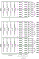
Fig. 22 shows the contents of the register G # 0 of the DPEs 0 through 7 in which each array d, G is stored by the storage unit 53 when the forward processing is performed.
In the DPE0, each of a plurality of computation cores computes a convolution between the matrices d and g stored in the corresponding one of the banks R # 0 to R # 7. Since the convolution is calculated in parallel in a plurality of calculation cores, the calculation speed of the convolution can be increased. This is also the case for DPE1 to DPE 7.
The array d of the arrays d and g is stored in the banks R # 0 to R # 7 of the DPEs 0 to 7 by the sequential method in the same manner as fig. 13. Here, only the Cin has the samemajorAre simultaneously stored in the banks R # 0 to R # 7. Then, after the convolution of array d is completed, there will be a different CinmajorArray d of (2) is stored in banks R # 0 to R # 7. FIG. 22 assumes having CinmajorCase where the array d of 0 is stored in the banks R # 0 to R # 7.
In this case, in the present embodiment, since Cin is shown as expression (5)minorIs the lowest level index of array d, and NminorIs a higher level index, so each bank is at the same NminorCin in the rangeminorAnd correspond to each other. Therefore, when Cin is presentminorTotal number of (2) is q (═ 4)Input channel number (Cin)major,Cinminor) Different from each other and lot number (N)major,Nminor) The same q sub-base matrices d are stored in q banks in one DPE.
For example, in the DPE0, four sub-bottom matrices d having a lot number N of (0, 0) and an input channel number Cin of (0, 0), (0, 1), (0, 2), and (0, 3) are stored in four (═ q) banks R # 0 to R # 3.
Therefore, unlike the case where the lot number N is changed with respect to each of the banks R # 0 to R # 7 as shown in fig. 13, q computation cores can compute the convolution of q sub-base matrices d having the same lot number N in parallel.
On the other hand, the storage unit 53 stores the weight matrix g in each bank of the DPEs 0 to 7 from the main memory 11 by a multicast method in the same manner as the example of fig. 13.
Here, the storage unit 53 stores a weight matrix g having the same input channel number Cin as the sub-base matrix d in each bank of each of the DPEs 0 to 7. By storing the matrices d and g in which the input channel numbers Cin are equal to each other in the same bank, the calculation unit 54 can calculate the convolution between the matrices d and g in which the input channel numbers Cin are equal to each other as shown in fig. 2.
However, as described with reference to fig. 15, when the array g is transferred to each bank by the multicast method, the regularity between the input lane number Cin and the output lane number Cout in one bank is lowered. Therefore, in the present embodiment, when calculating the convolution using the Winograd algorithm, the calculation unit 54 sorts the elements of the array g as follows.
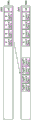
Fig. 23A to 25 show the contents of registers G # 0 to G # 3 of the DPE0 when the calculation unit 54 calculates convolution using the Winograd algorithm. In fig. 23A to 25, only the bank R # 0 of the registers G # 0 to G # 3 is shown to prevent the drawings from becoming complicated.
Before calculating the convolution, as shown in fig. 23A, the elements of the arrays d and G are stored in the bank R # 0 of the register G # 0. With different above-mentioned batch numbers N (═ N)major,Nminor) A plurality of arrays d of) are stored as the arrays dStored in the bank R # 0.
Then, according to equation (2), the array d is multiplied by the matrix B from both sides of the array dTAnd B, and the matrix B thus obtainedTdB is stored in the row that still stores array d. Matrix BTAnd elements of B are stored in constant region cst of bank R # 0.
At this time, the array g representing the weight matrix has a rule of disorder as shown in fig. 15.
Therefore, in the next step, as shown in fig. 23B, each element of the array G stored in the bank R # 0 of the register G # 0 is sorted by transferring the element to the bank R # 0 of the register G # 3.
In the register after sorting, as shown in fig. 16, banks R #0 to R # 7 are in one-to-one correspondence with output lane numbers Cout, and only elements of which Cout is 0 are stored in the bank R # 0.
Then, as shown in FIG. 24, the array G is multiplied by the matrices G and G from both sides of the array G according to equation (2)TAnd the matrix GgG thus obtainedTStored in free space of the memory bank. Matrices G and GTIs stored in the constant region cst of the bank R # 0.
Then, as shown in fig. 25, two matrices B in the bank R # 0 of the register G # 0 are mappedTdB and a matrix GgG in bank R # 0 of register G # 3TPerforming the element-by-element multiplication of equation (2)
Convolution is performed on two matrices with the same input channel number Cin as described with reference to fig. 2. Thus, four matrices GgG in bank R # 0 of register G # 3 are usedTThe matrix of which Cin is 0 and the bank R # 0 of the register G # 0minorTwo matrices B of 0TdB to perform element-by-element multiplication
Thereafter, according to equation (2), will From
From Are multiplied by the matrix aTAnd a to obtain a sub-top matrix y.
Through the above processing, the calculation of convolution using the Winograd algorithm performed by the calculation unit 54 is completed.
According to the foregoing convolution calculation, as shown in fig. 23A, there are different lot numbers N (═ N (N)minor,Nmajor) ) is stored in bank R # 0 of register G # 0.
Therefore, compared to the example in which a plurality of sub-base matrices d having the same lot number N and different input channel numbers Cin are stored in the same bank as described in fig. 17, the number of sub-base matrices d stored in one bank is reduced. As a result, the size t of the bottom matrix d can be increased, and the convolution can be calculated at high speed using the Winograd algorithm.
When the inventors tried for the case where t is 6, in the examples of fig. 3A to 3C in which the Winograd algorithm was not used, the time required for convolution was 2304 cycles. In contrast, the calculation time of the present embodiment is 1264 cycles, which indicates that the calculation speed is improved by 1.82(═ 2304/1264) times.
To further increase the computation speed of the convolution, the value of t is made as large as possible. However, when t is made too large, it becomes impossible to store the sub-base matrix d in each of the banks R # 0 to R # 7. On the other hand, when the value of t is small, the sub-base matrix d can be reliably stored in each of the banks R # 0 to R # 7, but the calculation time of convolution becomes long.
Therefore, in the present embodiment, the optimal value of t is obtained as follows. First, parameters are defined as follows.
p: number of memory banks in one DPE
q: storage in a DPE with the same NminorOf the sub-bottom matrix d
R: number of data sets that can be stored in one memory bank
In the case of the example of fig. 22, specific values of these parameters are as follows.
p:8
q:4
R:128
Further, the following parameters are defined.
Cin': number of input channel numbers Cin to be processed simultaneously in DPE0
Cout': the number of output channel numbers Cout to be processed simultaneously in DPE0
N': number of lots N to be processed simultaneously in DPE0
These parameters will be described with reference to the example of fig. 22.
Cin' is the number of input channel numbers Cin to be processed simultaneously in the DPE0 as described above. Input channel number Cin is composed ofmajor,Cinminor) And (5) identifying. However, since processing is only in DPE0 in the example of fig. 22 (Cin)major,Cinminor) The arrays g and d of (0, 0), (0, 1), (0, 2) and (0, 3) are set, so Cin' is 4.
On the other hand, Cout' is the number of output channel numbers Cout to be processed simultaneously in DPE0 as described above. In the example of fig. 22, since eight weight matrices g having a value of Cout of 0 to 7 are stored in the DPE0, Cout' is 8.
Further, N' is the number of lot numbers N to be processed simultaneously in the DPE0 as described above. In the example of fig. 22, since the combination (N) is processed in the DPE0major,Nminor) Four sub-base matrices d of (0, 0), (0, 1), (1, 0), (1, 1), so N' is 4. Next, the computation time of the convolution will be checked.
First, it will be checked to obtain a matrix B from the sub-base matrix d of t × t as shown in FIG. 23ATComputation time in dB. To obtain a matrix BTdB, e.g. first calculating BTd, and then multiplying the calculation result by the matrix B from the right side of the calculation result. To calculate BTd, decomposing the sub-bottom matrix d of t x t into t column vectors, and calculating the column vectors and the matrix BTThe product of (a).
Thus, in this example, one of the t column vectors and matrix B used to compute the sub-base matrix d that constitutes t TTThe calculation time required for the product of (a) is represented by b (t). B is obtained in a DPE by using the function B (t)TThe calculation time required for dB is represented by the following expression (6).

The reason why expression (6) includes "t" is that: because of the need to put the matrix B into operationTMultiplying by t column vectors of the sub-base matrix d to obtain BTd, so a computation time t times as long as the computation time represented by the function b (t) is required. Similarly, matrix B needs to be dividedTMultiplying d by t column vectors of the matrix B to obtain the matrix BTThe product of d and B. Therefore, the total calculation time becomes (t + t) times the calculation time represented by the function b (t). Therefore, expression (6) includes the factor "t + t".
Further, as shown in fig. 22, since Cin '· N' sub-base matrices d are in one DPE, the number of sub-base matrices d per bank becomes Cin '· N'/q. Since each of the compute cores C # 0 through C # 7 needs to compute B for each of the Cin '. N'/q sub-base matrices d in the corresponding bankTdB, therefore expression (6) includes the factor Cin.N'/q.
Next, it will be examined to obtain a matrix GgG from the 3 × 3 weight matrix g as shown in FIG. 24TThe calculation time of the hour.
To obtain the matrix GgGTFor example, first Gg is calculated, and then the calculation result is multiplied by the matrix G from the right of the calculation resultT. To calculate Gg, the weight matrix G is decomposed into three column vectors, and the product of the column vectors and the matrix G is calculated.
Therefore, in this example, the calculation time required for obtaining the product of one of the three column vectors constituting the 3 × 3 weight matrix G and the matrix G is represented by w (t). GgG are obtained in a DPE by using the function w (t)TWhen required calculationThe space is represented by the following expression (7).

The reason why expression (7) includes "3" is that: since the matrix G needs to be multiplied by three column vectors of the weight matrix G to obtain the matrix Gg, a calculation time three times as long as the calculation time represented by the function w (t) is required.
In addition, to obtain the matrix Gg and the matrix GTThe matrix Gg needs to be multiplied by the matrix GTT column vectors. Therefore, the total calculation time becomes (t +3) times as long as the calculation time represented by the function w (t). Therefore, expression (7) includes the factor "t + 3".
In addition, as shown in fig. 22, since Cin '· Cout' weight matrices g are in one DPE, the number of weight matrices g in one bank becomes Cin '· Cout'/p. Since each of the computation cores C # 0 to C # 7 needs to obtain GgG for each of Cin '. Cout'/p weight matrices g in the corresponding bankTThus, expression (7) includes the factor Cin 'Cout'/p.
Next, as shown in FIG. 25, the matrix B is examinedTdB and GgGTThe computation time required to perform the element-by-element multiplication.
As shown in fig. 22, the number of sub-base matrices d stored in one DPE is N ' · Cin '. Cout '/p. In addition, the number of elements of the sub-base matrix d is t2. Therefore, when in matrix BTdB and GgGTThe number of multiplications when element-by-element multiplication is performed is represented by the following expression (8).

Expressions (6) to (8) are calculation times when N ' lot numbers are selected from N lot numbers, Cout ' output lane numbers are selected from Cout output lane numbers, and Cin ' input lane numbers are selected from Cin input lane numbers. Therefore, in order to calculate the convolution between all the bottom matrices and all the weight matrices in fig. 2, it is necessary to perform the calculation as many times as the number of times represented by the following expression (9).

Factor HW/(t-2) in expression (9)2Indicates the total number of ways to partition the t × t sub-matrices from the H × W base matrix.
According to the above expressions (6) to (9), the calculation time depends not only on t but also on q. Therefore, in the present embodiment, the calculation time when convolution is calculated in one DPE is represented by the first function f (t, q). The first function f (t, q) is represented by the following expression (10) by multiplying the sum of expressions (6) and (7) by expression (9).

In order to reduce the computation time required for convolution, it is necessary to find the combination of t and q that minimizes the value of the first function f (t, q) on the condition that the number of elements in the weight matrix g and the sub-base matrix d does not exceed the number of elements that can be stored in the register.
Therefore, the number of elements of the sub-base matrix d and the weight matrix g will be checked next. First, the number of elements of the sub-base matrix d will be described.
Number of elements E of sub-bottom matrix d in one bank of one DPEbRepresented by the following equation (11).

In equation (11), t2Representing the number of elements of one sub-base matrix d. Cin 'N'/q represents the number of sub-base matrices d to be stored in one bank.
On the other hand, a DNumber E of elements of weight matrix g in one memory bank of PEwRepresented by the following equation (12).

In equation (12), 32Is the number of elements of a weight matrix g. In addition, Cin '. Cout'/p is the number of weight matrices g to be stored in one bank.
Based on equation (11) and equation (12), a second function g (t, q) representing the total number of elements of the sub-base matrix d and the weight matrix g is represented by equation (13) below.

As described above, when the number of data sets that can be stored in one bank is R as described above, the constraint represented by the following equation (14) is obtained.

Therefore, the calculation speed of convolution can be improved by finding the combination of t and q that minimizes the value of the first function f (t, q) represented by expression (10) from the combination of t and q that satisfies the constraint condition of equation (14).
Therefore, in the present embodiment, the calculation unit 42 calculates a combination of t and q that minimizes the value of the first function f (t, q) represented by expression (10) among combinations of t and q that satisfy the constraint condition of equation (14).
In the present embodiment, since R is 128, there are not many candidate combinations of t and q that satisfy equation (14). Therefore, the calculation unit 42 can find a combination of t and q satisfying equation (14) by exhaustive search, and can identify a combination that minimizes the value of the first function f (t, q) of expression (10) from the found combinations.
In expression (10), b (t) and w (t) are regarded as known functions. Here, b (t) and w (t) can be obtained as described below.
First, a method of obtaining w (t) will be described. As described above, w (t) is the calculation time required to obtain the product of one of the three column vectors constituting the weight matrix G of 3 × 3 and the matrix G when computing Gg. When t is 6, the elements of the matrix G are represented by the following equation (15).

This matrix G can be transformed into equation (16) below.

The two matrices on the right side of equation (16) are defined as equations (17) and (18) below.


Therefore, to calculate Gg, G ' G is first calculated, and then, the calculated G ' G is multiplied by G "from the left of G ' G. Therefore, a method of calculating G' G will be described.
Hereinafter, one column g' of the weight matrix g of 3 × 3 is described as (g)0,g1,g2)T. Therefore, G' can be represented by the following equation (19).

Here, (x)0,x1,x2,x3,x4,x5)TIs a variable in which each element of G' is stored.
Here, in order to perform the calculation of equation (19), six array elements a [0] are prepared]、a[1]、a[2]、a[3]、a[4]And a [5 ]]. Then, g is mixed0、g1And g2Are respectively stored in a [0]]、a[1]And a [2]]In (1). Then, two array elements b [0] are prepared]And b [1]]As a buffer for calculations.
In this case, equation (19) may be calculated by inserting the values for each array element in the order of fig. 26.
Fig. 26 is a diagram showing the calculation of equation (19) in order of steps. Here, "//" in fig. 26 is an annotation indicating the meaning of each step. The same applies to fig. 27 described later.
When the calculation is performed according to the sequence shown in FIG. 26, (a [0] ends],a[1],a[2],a[3],a[4],a[5])=(x0,x1,x5,x2,x4,x3) And the calculation result of G 'G' can be stored in the array element a [0]]、a[1]、a[2]、a[3]、a[4]And a [5 ]]In each of which.
G' can be calculated in eight steps. Therefore, w (6) is 8. Even when the value of t is different from 6, the value of w (t) can be obtained in the same manner as described above.
Next, a method of obtaining b (t) will be described. As mentioned above, B (t) is one of the t column vectors and the matrix B for obtaining the sub-base matrix d constituting t × tTProduct of (B)Td required calculation time. When t is 6, the matrix BTIs expressed by the following equation (20).

Further, hereinafter, one column d' of the 6 × 6 sub-base matrix d is described as (d)0,dl,d2,d3,d4,d5)T. In this case, BTd' can be expressed by the following equation (21)。

Here, (x)0,x1,x2,x3,x4,x5)TIs to store B thereinTd' of the elements.
Here, in order to calculate equation (21), six array elements a [0] are prepared]、a[1]、a[2]、a[3]、a[4]And a [5 ]]And d is0、d1、d2、d3、d4And d5Are respectively pre-stored in array elements a [0]]、a[1]、a[2]、a[3]、a[4]And a [5 ]]In (1).
In addition, four array elements b [0], b [1], b [2], and b [3] are prepared as buffers for calculation.
In this case, equation (21) may be calculated by inserting the values for each array element in the order of fig. 27.
Fig. 27 is a diagram showing the calculation of equation (21) in the order of steps. When the calculations are performed in the order shown in FIG. 27, finally (a [0]],a[1],a[2],a[3],a[4],a[5])=(x0,x1,x2,x3,x4,x5) And B isTThe result of the computation of d' may be stored in array element a [0]]、a[1]、a[2]、a[3]、a[4]And a [5 ]]In each of which.
Thus, B can be calculated in 15 stepsTd'. Therefore, b (6) is 15. Even when the value of t is different from 6, the value of b (t) can be obtained in the same manner as described above.
Based on the fact described above, the information processing apparatus 31 according to the present embodiment executes the following information processing method.
Fig. 28 is a flowchart of an information processing method according to the present embodiment. First, in step S1, the calculation unit 42 (see fig. 20) calculates a combination of t and q. For example, the calculation unit 42 calculates a combination that minimizes the value of the first function f (t, q) of the expression (10) among combinations of t and q that satisfy the constraint condition of equation (14). This makes it possible to obtain a combination that minimizes the calculation time from combinations of t and q that allow elements of the weight matrix g and the sub-base matrix d of t × t to be stored in q banks.
Then, in step S2, the output unit 41 (see fig. 20) outputs the program 50 executable by the computing machine 10 (see fig. 5).
The combination of t and q calculated in step S1 is used in the program 50. For example, when the computing machine 10 executes the program 50, the selection unit 52 (see fig. 21) selects the sub-bottom matrix d of t × t from the bottom matrix.
Then, the storage unit 53 stores the sub-bottom matrix d and the weight matrix g of t × t in q banks of the banks R # 0 to R # 7 of the DPE 0. Thereafter, the calculation unit 54 calculates the convolution between the sub-base matrix d and the weight matrix g using the Winograd algorithm according to the process of fig. 23A to 25.
Through the above processing, the basic steps of the information processing method according to the present embodiment are completed.
According to the embodiment described above, the calculation unit 42 calculates a combination of t and q that minimizes the first function f (t, q) representing the calculation time of convolution under the constraint condition of equation (14) that can store the sub-base matrix d and the weight matrix g in one memory bank.
Therefore, when the sub-base matrix d and the weight matrix g are stored in the bank of the register, the convolution can be calculated at high speed using the sub-base matrix d and the weight matrix g.
Backward processing
In the example of fig. 22, the Winograd algorithm is used to compute the convolution in the forward process of deep learning.
Hereinafter, a Winograd algorithm in the backward processing of the deep learning will be described. The backward processing includes a process of obtaining a bottom matrix by convolution between a top matrix and a weight matrix and a process of obtaining a weight matrix by convolution between a top matrix and a bottom matrix.
First, a process of obtaining the bottom matrix by convolution between the top matrix and the weight matrix will be described.
Fig. 29A to 29C are diagrams when convolution between the top matrix and the weight matrix is calculated using the Winograd algorithm in the backward processing.
First, as shown in fig. 29A, the selection unit 52 (see fig. 21) selects a sub top matrix y of t × t from the top matrix of H rows and W columns.
Then, the calculation unit 54 obtains the sub-bottom matrix d by convolution between the weight matrix g and the sub-top matrix y according to the following equation (22).
d=AT{(GgGT)◎(BTyB)}A…(22)
Then, as shown in fig. 29B, the position of dividing the sub-top matrix y from the top matrix is shifted by two columns from the position of the case of fig. 29A, and the divided sub-top matrix y is subjected to the same calculation as described above. The resulting sub-base matrix d forms a block in the base matrix adjacent to the sub-base matrix d obtained in fig. 29A.
As described above, by repeatedly shifting the position of the sub top matrix y divided from the matrix by two columns and two rows, the bottom matrix formed of the sub bottom matrix d is obtained as shown in fig. 29C.
Through the above steps, the calculation of the convolution between the top matrix and the weight matrix in the backward processing is completed. In this example, the weight matrix g is an example of a first matrix, and the sub-top matrix y of t × t is an example of a second matrix.
Next, the function of the storage unit 53 when the backward processing is performed in the above-described manner will be described in detail.
The storage unit 53 sorts the elements of each array as represented by the following expression (23), and stores the elements in the banks R # 0 to R # 7 of the DPEs 0 to 7.

Here, when N is a lot number, (the number of N) ═ NmajorNumber of (A) × (N)minor(number of Cout) ═ Cout (number of Cout)majorNumber of (1) × (Cout)minorThe number of (d). In this case, the lot number N is composed of combinations (N) as in expression (5)major,Nminor) And (5) identifying. In the backward processing, the batch number N is an example of a second identifier for identifying the child top matrix y.
The output channel number Cout is also combined (Cout)major,Coutminor) And (5) identifying. For example, Coutmajor=0,CoutminorThe array element of 0 corresponds to Cout 0, and Coutmajor=0,CoutminorThe array element of 1 corresponds to Cout 1. Further, in the backward processing, the output channel number Cout is a first identifier for identifying the sub-top matrix y.
Further, in this example, as in fig. 2, it is assumed that the total number of lot numbers N is 64, and the total number of output lane numbers Cout is 384. Also assume NmajorTotal number of (1) is 16, and CoutminorThe total number of (a) is 4.
The elements [ H "] [ W" ] in the array y correspond to the elements of the sub-top matrix y of t x t.
Fig. 30 shows the contents of the register G # 0 of the DPEs 0 through 7 in which the arrays y and G are stored by the storage unit 53.
The array y is stored in the banks R # 0 to R # 7 of the DPEs 0 to 7 by the memory cell 53 through a sequential method.
In this case, in the present embodiment, Cout is as shown in expression (23)minorIs the lowest level index of array y, and NminorIs the next higher level index. Thus, each bank is associated with the same NminorCout within rangeminorAnd correspond to each other. Therefore, when CoutminorHas a different output channel number (Cout) when the total number of (c) is q (═ 4)major,Coutminor) And the same lot number (N)major,Nminor) Q sub-top matrices y are stored in q banks of one DPE.
For example, in the DPE0, four sub top matrices y having the lot number N of (0, 0) and the output channel number Cout of (0, 0), (0, 1), (0, 2), (0, 3) are stored in the four banks R # 0 to R # 3, respectively.
Therefore, unlike the example in which the lot number N is changed with respect to each of the banks R # 0 to R # 7 as shown in fig. 13, the convolution of q sub top matrices y having the same lot number N can be calculated in parallel in q calculation cores.
On the other hand, as in the example of fig. 22, the weight matrix g is transferred from the main memory 11 to the DPEs 0 to 7 by the multicast method by the storage unit 53.
As described with reference to fig. 15, in the multicast method, there is no regularity between the value of the input lane number Cin and the value of the output lane number Cout. Therefore, also in this example, the calculation unit 54 sorts the array g as in fig. 23A to 25.
Next, the computation time of convolution in this backward processing will be checked.
B represented by equation (22) is obtained in one DPETThe calculation time required for yB can be expressed by the following expression (24) by replacing Cin 'in expression (6) with Cout'.

In addition, GgG expressed by equation (22) is obtained in one DPE for the same reason as that of expression (7)TThe required calculation time can be represented by expression (25).

Further, matrix B is formed in the execution of equation (22)TyB and GgGTThe number of multiplications in the element-by-element multiplication therebetween is represented by the following expression (26) as with the expression (8).

In order to calculate the convolution between all top matrices and all weight matrices, it is necessary to perform the calculation as many times as the number of times expressed by the following expression (27), where p in the expression (9) is replaced with Cout'.

The first function f (t, q) representing the calculation time when convolution is calculated in one DPE can be represented by the following equation (28) by multiplying the sum of expressions (24) to (26) by expression (27).

Next, the condition that the number of elements of the sub-top matrix y and the weight matrix g does not exceed the number of elements that can be stored in the register will be checked. First, the number of elements of the sub-top matrix y will be described.
Number E of elements of sub-top matrix y in one bank of one DPEyCan be expressed by the following equation (29) by replacing Cin 'in equation (11) with Cout'.

On the other hand, as with equation (12), the number E of elements of the weight matrix g in one bank of one DPE can be expressed by the following equation (30)w。

Based on equation (29) and equation (30), the second function g (t, q) representing the total number of elements of the sub-top matrix y and the weight matrix g can be represented by equation (31) below.

Therefore, when the number of data sets stored in one bank is R, the constraint represented by the following equation (32) is obtained.

Therefore, the calculation speed of convolution can be improved by finding the combination of t and q that minimizes the value of the first function f (t, q) of equation (28) from the combination of t and q that satisfies the constraint condition of equation (32).
Therefore, when performing backward processing for obtaining the sub-bottom matrix d by convolution between the top matrix and the weight matrix, the calculation unit 42 identifies a combination of t and q that satisfies the constraint condition of equation (32). Then, the calculation unit 42 calculates a combination of t and q that minimizes the value of the first function f (t, q) of equation (28) among the identified combinations to increase the calculation speed of convolution.
Next, a backward process for obtaining a weight matrix by convolution between the top matrix and the bottom matrix will be described.
Fig. 31A to 32C are diagrams when convolution between the top matrix and the bottom matrix is calculated using the Winograd algorithm in the backward process.
First, as shown in fig. 31A, the selection unit 52 selects a sub top matrix y of t '× t' from the top matrix of H × W.
Then, as shown in fig. 31B, the selection unit 52 selects a sub-bottom matrix d of (t '-2) × (t' -2) from the bottom matrix of H '× W'.
Then, as shown in fig. 32A, the calculation unit 54 selects a matrix y ' of (t ' -2) × (t ' -2) from the sub top matrix y. Then, the calculation unit 54 obtains 11 components of the weight matrix g according to the following equation (33).
g11=AT{(Gy′GT)◎(BTdB)}A…(33)
Then, as shown in fig. 32B, the position at which the matrix y 'is selected from the sub-top matrix y is shifted by one column from the position in the case of fig. 32A, and the calculation unit 54 performs the same calculation as the above-described calculation on the selected matrix y' to obtain 12 components of the weight matrix g.
As described above, each element of the weight matrix g of 3 × 3 as shown in fig. 32C is obtained by repeatedly moving the position of the division matrix y' from the sub-top matrix y in the column direction and the row direction.
Through the above processing, the calculation of the convolution between the top matrix and the bottom matrix in the backward processing is completed. In this example, the sub-bottom matrix d of (t '-2) × (t' -2) is an example of the first matrix, and the sub-top matrix y of t '× t' is an example of the second matrix.
Next, the function of the storage unit 53 when the backward processing is performed will be described in detail.
The storage unit 53 sorts the elements of each array represented by the following expression (34), and then stores each element to the banks R # 0 to R # 7 of the DPEs 0 to 7.

Also in this example, the sub-base matrix d is passed through the lot number N (═ N)major,Nminor) And an input channel number Cin (═ Cin)major,Cinminor) ) are identified. Lot number N (═ N)major,Nminor) Is an example of the first identifier, and the input channel number Cin (═ Cin)major,Cinminor) Is an example of the second identifier.
Fig. 33 shows the contents of the register G # 0 of the DPEs 0 to 7 in which the arrays y and d are stored by the storage unit 53.
The array d is stored in the banks R # 0 to R # 7 of the DPEs 0 to 7 by the sequential method by the memory cell 53.
In this case, in the present embodiment, since N is shown as expression (34)minorIs the lowest level index of array d, and CinminorIs the next higher level index. Thus, each bank is associated with the same CinminorN within the rangeminorOne-to-one correspondence. Therefore, when N isminorWhen the total number of (c) is q (═ 4), it will have different lot numbers (N)major,Nminor) And the same input channel number (Cin)major,Cinminor) Q sub-base matrices d are stored in q banks of one DPE.
For example, four sub-base matrices d having an input channel number Cin of (0, 0) and a lot number N of (0, 0), (0, 1), (0, 2), (0, 3) are stored in the four banks R # 0 to R # 3 of the DPE0, respectively.
Therefore, unlike the example in which the lot number N is changed with respect to each of the banks R # 0 to R # 7 as shown in fig. 13, the convolution of q sub-base matrices d having the same input channel number Cin can be calculated in parallel by q calculation cores.
The sub-top matrix y is transferred from the main memory 11 to the DPEs 0 to 7 by the storage unit 53 through a multicast method.
Unlike the example of fig. 30, in this example, Cout is shown in expression (34)minorIs the lowest level index of array y, and NminorIs the next higher level index. In addition, let Cout beminorIs 4, and NminorThe total number of (a) is 4.
Thus, for example, in DPE0, with CoutminorAscending order of values will be N major0 and NminorElements of the array y of 0 are stored in the banks R # 0 to R # 3. Then, with CoutminorAscending order of values will be N in the array major0 and NminorThe element of 1 is stored in the banks R # 4 to R # 7.
N in array ymajorThe element 1 is also represented by CoutminorThe ascending order of values is stored in the banks R # 0 to R # 3, and NminorElements that are 1 large are stored in banks R # 4 to R # 7.
Thus, have the same CoutminorThe elements of the array y of values are stored in one memory bank. Thus, it is not necessary to sort the elements of array y to get Cout in the bankminorThe values are the same.
Next, the computation time of convolution in this backward processing will be checked.
Gy' G represented by equation (33) is obtained in one DPETThe required calculation time will be represented by the following expression (35) by replacing t in expression (24) with t'.

Further, for obtaining B represented by equation (33) in one DPETThe calculation time of dB will be represented by the following expression (36) by replacing 3, t and cout 'in the expression (25) with t' -2, t 'and N', respectively.

Further, in equation (33), when the matrix Gy' G is executedTAnd matrix BTThe number of multiplications at element-by-element multiplication between dbs is represented by the following equation (37) as with expression (8).

In order to calculate the convolution between all the top matrices and all the weight matrices, it is necessary to perform the calculation as many times as expressed by expression (38) below, which is the same as expression (27).

The first function f (t, q) representing the calculation time when convolution is calculated in one DPE can be represented by the following equation (39) by multiplying the sum of expressions (35) to (37) by expression (38).

Next, the condition that the number of elements of the sub-bottom matrix d and the sub-top matrix y does not exceed the number of elements that can be stored in the register will be checked.
First, the number of elements of the sub-top matrix y will be described. Number E of elements of sub-top matrix y in one bank of one DPEyCan be represented by the following equation (40).

T 'in equation (40)'2Is the number of elements of a sub-top matrix y. In addition, N '. Cin'/p is the number of sub top matrices y to be stored in one bank.
On the other hand, the number E of elements of the sub-bottom matrix d in one bank of one DPEdCan be expressed by the following equation (41).

In equation (41), (t' -2)2Is the number of elements of one sub-base matrix d. In addition, N '· Cout'/p is the number of sub-bottom matrices d to be stored in one bank.
Based on equation (29) and equation (30), the second function g (t, q) representing the total number of elements of the sub-top matrix y and the weight matrix g can be represented by equation (42) below.

Therefore, when the number of data sets that can be stored in one bank is R, the constraint represented by the following equation (43) is obtained.

Therefore, the calculation speed of convolution can be improved by finding the combination of t and q that minimizes the value of the first function f (t, q) of equation (39) from the combination of t and q that satisfies the constraint condition of equation (43).
Accordingly, when performing the backward processing of obtaining the weight matrix by convolution between the bottom matrix and the top matrix as described in the present example, the calculation unit 42 identifies the combination of t and q that satisfies the constraint condition of equation (43). Then, the calculation unit 42 calculates a combination of t and q that minimizes the value of the first function f (t, q) of equation (39) among the identified combinations to increase the calculation speed of convolution. 1 x 1 convolution
In the deep learning, 1 × 1 convolution may be performed. For example, ResNet-50 or ResNet 101 uses a 1 × 1 convolution. Therefore, 1 × 1 convolution in the present embodiment will be described.
Although there is no particular limitation on the matrix to be subjected to the 1 × 1 convolution, hereinafter, the convolution between the sub-base matrix d and the weight matrix g will be described.
When performing 1 × 1 convolution between the matrices d and g, the storage unit 53 stores the elements of each matrix in the corresponding array represented by expression (44), and stores the elements in the banks R # 0 to R # 7 of the DPEs 0 to 7.

The order of the elements of each array d, g in expression (44) is the same as that of expression (5). For example, in array d, CinminorIs the lowest level index, and NminorIs the next higher level index.
Fig. 34 shows the contents of register G # 0 of DPE0 in which arrays d and G are stored by storage unit 53 when performing 1 × 1 convolution.
In the case of expression (5), as shown in fig. 22, array d is stored in DPEs 0 to 7 by a sequential method, however, in this example, array d is stored in DPEs 0 to 7 by a multicast method.
Thus, for example, N major0 and N minor0 in CinminorThe order of 0, 1, 2, 3 is stored in the banks R # 0, R # 1, R # 2, and R # 3. When N is storedmajor0 and NminorWhen all elements are equal to 0, then N is addedmajor0 and N minor1 in CinminorThe order of 0, 1, 2, 3 is stored in memory banks R #4, R # 5, R # 6, and R # 7. Accordingly, the first row of each of the banks R # 0 to R # 7 is filled, and thus, NminorElements of 2 or greater are stored in the next row.
After completing to NmajorAfter convolution of the element 0, N is addedmajorThe elements of array d, 1, are extended to DPE 0. The same applies to NmajorElements of array d being 2 or greater than 2.
In addition, for the array g, the array g is stored in the bank R # 0 by the multicast method.
There is no Winograd algorithm applicable to the 1 × 1 convolution. Therefore, in this example, the calculation unit 54 performs convolution according to the procedure illustrated in fig. 3A to 3C by using the elements stored in the banks R # 0 to R # 7.
Batch normalization
In deep learning, performance may be improved by performing batch normalization. Batch normalization is a normalization method of making the average value of pixel data of each image 0 and making the distribution of pixel data 1 when the value of pixel data is greatly different among a plurality of images. The method will be described hereinafter.
When performing batch normalization, the storage unit 53 sorts the elements of each array d, y as shown in the following expression (45), and stores the elements in the banks R # 0 to R # 7 of the DPEs 0 to 7 by a multicast method.

Batch normalization is applicable to both the bottom and top matrices. Hereinafter, a case where batch normalization is performed on the sub-base matrix d which is a part of the base matrix will be described.
Fig. 35 shows the contents of the register G # 0 of the DPE0 in which the sub-bottom matrix d is stored by the storage unit 53 when batch normalization is performed.
In this example, as in fig. 34, the storage unit 53 stores the sub-base matrix d in the bank R # 0 by the multicast method. Cin as shown in expression (45)minorIs the lowest level index of the sub-base matrix d. Therefore, when looking at one of the banks R # 0 to R # 7, have the same CinminorThe elements of the value are stored in one memory bank. For example, Cin aloneminorAn element of 0 is stored in the bank R # 0.
In addition, according to expression (45), in the sub-base matrix d, NminorIs the grade ratio CinminorThe high index. Therefore, when looking at one of the banks R # 0 to R # 7, it has a different lot number (N)major,Nminor) Is stored in a memory bank. For example, having (N)major,Nminor) Elements of ═ 0, 0), (0, 2), … (0, 14), (1, 0), (1, 2), … (1, 14), … (3, 0), (3, 2), … (3, 14) are stored in the bank R # 0.
As described above, have the same CinminorAnd different lot numbers (N)major,Nminor) Is stored in a memory bank. Therefore, each of the computation cores C # 0 to C # 7 can compute having the same Cin by using only the corresponding one bankminorAnd different lot numbers (N)major,Nminor) And dispersion (dispersion) of these elements.
The calculation is performed by the calculation unit 54 as follows. Fig. 36A and 36B show the contents of the register G # 0 of the DPE0, and are diagrams for describing the calculation performed by the calculation unit 54 when batch normalization is performed.
First, as shown in fig. 36A, the computation core C # 0 adds up the values of the elements of the sub-bottom matrix d in the bank R # 0, and obtains the value x0Line L stored in bank R # 0sum_1In (1). Also in the other banks R #1 to R # 7, the counterEach of the kernels C # 1 to C # 7 adds up the values of the elements of the sub-bottom matrix d in the corresponding bank, and then adds up the obtained value x1To x7Lines L stored in banks R # 1 to R # 7, respectivelysum_1。
Here, as shown in FIG. 35, only NminorElements that are even numbers are stored in the bank R # 0. Thus, the value x0Become not all lot numbers (N)major,Nminor) Is the sum of elements of (a) and is NminorIs the sum of the values of the elements of even numbers.
Thus, the calculation unit 54 calculates the value x0To x7Is of the same Cin as CinminorThe corresponding values are added. For example, the value x0Sum value x4Both correspond to Cin minor0. Therefore, the calculation unit 54 adds these two values and writes the result to the value x0. The obtained value x0Equal to across all lot numbers (N)major,Nminor) C is to mix CinminorThe elements of 0 are added to obtain the value. Similarly, the calculation unit 54 performs the following calculation.
x1=x1+x5
x2=x2+x6
x3=x3+x7
Then, the computing core C # 0 passes the value x to be stored in the memory bank R # 00Divide by batch number to calculate the average m0And the obtained average value m0Line L stored in bank R # 0meanIn (1). Also in the banks R # 1 to R # 3, the computation cores C # 1 to C # 3 respectively compute the value x1To x3Average value m of1To m3And stores these values in rows L of the banks R # 1 to R # 3, respectivelymeanIn (1).
Through the above processing, the average values m of the elements of the sub-bottom matrix d are obtained for the banks R # 0 to R # 3, respectively0To m3. Next, a method of calculating dispersion will be described.
First, as shown in fig. 36B, the computation core C # 0 pairs each element of the sub-bottom matrix d in the bank R #0And a value y obtained by summing the obtained values is squared and0line L stored in bank R # 0sum_2In (1). Also in the other banks R #1 to R # 7, each of the computation cores C # 1 to C # 7 squares the value of each element in the corresponding bank, sums the obtained values, and sums the obtained value y1To y7Line L stored to a corresponding bank among the banks R # 1 to R # 7sum_2。
As in the example of FIG. 36A, the value y0Not across all batch numbers (N)major,Nminor) Is the sum of the squares of the values of the elements of (b), but only by pairs-as NminorSquared-value of the values of the elements of even numbers. Thus, the calculation unit 54 performs the following calculation, and will span all the lot numbers (N)major,Nminor) Is written at the value y0To y3In (1).
y0=y0+y4
y1=y1+y5
y2=y2+y6
y3=y3+y7
Then, the computing core C # 0 passes the value y to be stored in the memory bank R # 00Divide by lot number to calculate the average a0And calculating the average value a0Line L stored in bank R # 0mean_2In (1). Also in the banks R # 1 to R # 3, the computation cores C # 1 to C # 3 compute the value y1To y3Average value of (a)1To a3And stores these values in rows L of the banks R # 1 to R # 3, respectivelymean_2In (1).
Through the above processing, the average value a of the squares of the elements of the sub-bottom matrix d is obtained for the banks R # 0 to R # 30To a3。
Then, the calculation unit 54 calculates v0=a0-m0 2To calculate the dispersion v of the elements of the sub-base matrix d of the bank R # 00And then will be releasedDifference v0Line L stored in bank R # 0varIn (1). In the same manner, the calculation unit 54 performs the following calculation to calculate the dispersion v of the elements of the banks R # 1 to R # 31To v3And will deviate from the difference v1To v3Are stored in rows L of the memory banks R #1 to R # 3, respectivelyvarIn (1).
v1=a1-m1 2
v2=a2-m2 2
v3=a3-m3 2
Thereafter, the calculation unit 54 calculates the value (d [ N ] of each element of the sub-base matrix d by the following equation (46)major][Cinmajor][H][W][Nminor][i]) With the average value miThe difference between them divided by the dispersion viTo CinminorBatch normalization is performed for i ( i 0, 1, 2, 3).

Through the above processing, batch normalization is completed.
By performing batch normalization as described above, improvement in learning performance of deep learning is expected.
Although the illustrative embodiments of the present invention have been described in detail, the present invention is not limited to the above-mentioned embodiments, and other embodiments, variations, and modifications may be made without departing from the scope of the present invention.
Claims (9)
1. An information processing apparatus comprising:
a calculation unit that calculates a combination of t and q that minimizes a calculation time when q calculation cores calculate convolutions between a plurality of first matrices and a plurality of second matrices of t rows and t columns in parallel using a Winograd algorithm, wherein a total number of elements of the plurality of first matrices and the plurality of second matrices does not exceed a number of data sets that can be stored in each of q storage regions of a register, and the q calculation cores correspond to the q storage regions, respectively; and
an output unit that outputs a program for causing a computing machine to execute processing including: storing the plurality of first matrices and the plurality of second matrices in respective ones of the q storage areas using a combination of the calculated t and q, and calculating a convolution between the first matrix and the second matrix using the Winograd algorithm by each of the q computation cores, the computation machine including the q computation cores and the register.
2. The information processing apparatus according to claim 1,
each of the first matrix and the second matrix is a matrix in a deep-learned convolutional layer.
3. The information processing apparatus according to claim 1,
when the calculation time is represented by a first function f (t, q) and the total number of elements of the plurality of first matrices and the plurality of second matrices stored in one of the storage regions is represented by a second function g (t, q), the calculation unit calculates a combination of q and t that minimizes the value of the first function f (t, q) within a range in which the value of the second function g (t, q) does not exceed the number of data sets that can be stored in one storage region.
4. The information processing apparatus according to claim 3,
each of the first matrix and the second matrix is a matrix in a deep-learned convolutional layer, and
the first function f (t, q) and the second function g (t, q) in the backward processing of the deep learning are different from the first function f (t, q) and the second function g (t, q) in the forward processing of the deep learning, respectively.
5. The information processing apparatus according to claim 1,
each of the plurality of second matrices is identified by a combination of the first identifier and the second identifier, and
the program causes the computing machine to perform a process of storing each of q second matrices in each of the q storage areas, wherein the first identifiers of the q second matrices are different from each other and the second identifiers of the q second matrices are the same.
6. The information processing apparatus according to claim 5,
the program causes the computing machine to execute a process comprising:
storing the first matrix and the second matrix, in which the first identifiers are identical to each other, in the same storage area, and
calculating a convolution between the first matrix and the second matrix stored in the same memory area.
7. The information processing apparatus according to claim 1,
the program causes the computing machine to execute a process comprising:
calculating an average and a dispersion of the values of the elements for each of the plurality of storage areas, an
Normalizing, for each of the plurality of storage regions, a value of the element by dividing a difference between the value of the element and the average by the dispersion.
8. A non-transitory computer-readable storage medium storing an information processing program that causes a computer to execute a process, the process comprising:
calculating a combination of t and q that minimizes a calculation time when q calculation cores calculate convolutions between a plurality of first matrices and a plurality of second matrices of t rows and t columns in parallel using a Winograd algorithm, wherein a total number of elements of the plurality of first matrices and the plurality of second matrices does not exceed a number of data sets that can be stored in each of q storage regions of a register, and the q calculation cores correspond to the q storage regions, respectively; and
outputting a program for causing a computing machine to execute a process, the process comprising: storing the plurality of first matrices and the plurality of second matrices in respective ones of the q storage areas using a combination of the calculated t and q, and calculating a convolution between the first matrix and the second matrix using the Winograd algorithm by each of the q computation cores, the computation machine including the q computation cores and the register.
9. An information processing method implemented by a computer, the information processing method comprising:
calculating a combination of t and q that minimizes a calculation time when q calculation cores calculate convolutions between a plurality of first matrices and a plurality of second matrices of t rows and t columns in parallel using a Winograd algorithm, wherein a total number of elements of the plurality of first matrices and the plurality of second matrices does not exceed a number of data sets that can be stored in each of q storage regions of a register, and the q calculation cores correspond to the q storage regions, respectively; and
outputting a program for causing a computing machine to execute a process, the process comprising: storing the plurality of first matrices and the plurality of second matrices in respective ones of the q storage areas using a combination of the calculated t and q, and calculating a convolution between the first matrix and the second matrix using the Winograd algorithm by each of the q computation cores, the computation machine including the q computation cores and the register.
Applications Claiming Priority (2)
| Application Number | Priority Date | Filing Date | Title |
|---|---|---|---|
| JP2019119018A JP7251354B2 (en) | 2019-06-26 | 2019-06-26 | Information processing device, information processing program, and information processing method |
| JP2019-119018 | 2019-06-26 |
Publications (1)
| Publication Number | Publication Date |
|---|---|
| CN112149794A true CN112149794A (en) | 2020-12-29 |
Family
ID=70682683
Family Applications (1)
| Application Number | Title | Priority Date | Filing Date |
|---|---|---|---|
| CN202010466951.3A Pending CN112149794A (en) | 2019-06-26 | 2020-05-28 | Information processing apparatus, computer-readable storage medium, and information processing method |
Country Status (4)
| Country | Link |
|---|---|
| US (1) | US11631002B2 (en) |
| EP (1) | EP3757902A1 (en) |
| JP (1) | JP7251354B2 (en) |
| CN (1) | CN112149794A (en) |
Families Citing this family (1)
| Publication number | Priority date | Publication date | Assignee | Title |
|---|---|---|---|---|
| JP2023000031A (en) | 2021-06-17 | 2023-01-04 | 富士通株式会社 | Data arrangement program, processor, and data arrangement method |
Citations (2)
| Publication number | Priority date | Publication date | Assignee | Title |
|---|---|---|---|---|
| US20170132496A1 (en) * | 2015-11-05 | 2017-05-11 | Microsoft Technology Licensing, Llc | Hardware-efficient deep convolutional neural networks |
| US20170344876A1 (en) * | 2016-05-31 | 2017-11-30 | Samsung Electronics Co., Ltd. | Efficient sparse parallel winograd-based convolution scheme |
Family Cites Families (7)
| Publication number | Priority date | Publication date | Assignee | Title |
|---|---|---|---|---|
| JP5368687B2 (en) | 2007-09-26 | 2013-12-18 | キヤノン株式会社 | Arithmetic processing apparatus and method |
| US10482155B2 (en) * | 2016-12-30 | 2019-11-19 | Intel Corporation | Winograd algorithm on a matrix processing architecture |
| US10824938B2 (en) * | 2017-04-24 | 2020-11-03 | Intel Corporation | Specialized fixed function hardware for efficient convolution |
| JP6879072B2 (en) | 2017-06-21 | 2021-06-02 | コニカミノルタ株式会社 | Processing methods, programs, information processing equipment, and image processing equipment |
| US10990648B2 (en) * | 2017-08-07 | 2021-04-27 | Intel Corporation | System and method for an optimized winograd convolution accelerator |
| CN107993186B (en) * | 2017-12-14 | 2021-05-25 | 中国人民解放军国防科技大学 | 3D CNN acceleration method and system based on Winograd algorithm |
| CN108765247B (en) * | 2018-05-15 | 2023-01-10 | 腾讯科技(深圳)有限公司 | Image processing method, device, storage medium and equipment |
-
2019
- 2019-06-26 JP JP2019119018A patent/JP7251354B2/en active Active
-
2020
- 2020-05-12 EP EP20174274.9A patent/EP3757902A1/en active Pending
- 2020-05-28 CN CN202010466951.3A patent/CN112149794A/en active Pending
- 2020-05-28 US US16/885,332 patent/US11631002B2/en active Active
Patent Citations (3)
| Publication number | Priority date | Publication date | Assignee | Title |
|---|---|---|---|---|
| US20170132496A1 (en) * | 2015-11-05 | 2017-05-11 | Microsoft Technology Licensing, Llc | Hardware-efficient deep convolutional neural networks |
| CN108351984A (en) * | 2015-11-05 | 2018-07-31 | 微软技术许可有限责任公司 | The depth convolutional neural networks of hardware-efficient |
| US20170344876A1 (en) * | 2016-05-31 | 2017-11-30 | Samsung Electronics Co., Ltd. | Efficient sparse parallel winograd-based convolution scheme |
Non-Patent Citations (1)
| Title |
|---|
| FENG SHI等: "Sparse Winograd Convolutional neural networks on small-scale systolic arrays", FIELD-PROGRAMMABLE GATE ARRAYS 2019, pages 118 - 118 * |
Also Published As
| Publication number | Publication date |
|---|---|
| JP2021005242A (en) | 2021-01-14 |
| EP3757902A1 (en) | 2020-12-30 |
| JP7251354B2 (en) | 2023-04-04 |
| US20200410340A1 (en) | 2020-12-31 |
| US11631002B2 (en) | 2023-04-18 |
Similar Documents
| Publication | Publication Date | Title |
|---|---|---|
| US11720523B2 (en) | Performing concurrent operations in a processing element | |
| US11880768B2 (en) | Method and apparatus with bit-serial data processing of a neural network | |
| CN109324827B (en) | Apparatus, method and system for processing instructions for accessing data | |
| BR112019000541B1 (en) | COMPUTER-IMPLEMENTED IMAGE RECOGNITION METHOD FOR MORE EFFICIENTLY PERFORMING A CONVOLUTIONAL NEURAL NETWORK ONE-LAYER COMPUTATION, IMAGE RECOGNITION SYSTEM AND COMPUTER STORAGE MEDIUM | |
| US11144823B1 (en) | Method and system for hierarchical weight-sparse convolution processing | |
| US11580376B2 (en) | Electronic apparatus and method for optimizing trained model | |
| CN110796235B (en) | Vectorization implementation method for Valid convolution of convolutional neural network | |
| US11164032B2 (en) | Method of performing data processing operation | |
| US11763150B2 (en) | Method and system for balanced-weight sparse convolution processing | |
| EP4009243A1 (en) | Cluster-connected neural network | |
| Mao et al. | Energy-efficient machine learning accelerator for binary neural networks | |
| CN112149794A (en) | Information processing apparatus, computer-readable storage medium, and information processing method | |
| CN113516019A (en) | Hyperspectral image unmixing method and device and electronic equipment | |
| CN109614581A (en) | The Non-negative Matrix Factorization clustering method locally learnt based on antithesis | |
| CN111626368B (en) | Image similarity recognition method, device and equipment based on quantum algorithm | |
| CN114692854A (en) | NPU for generating kernel of artificial neural network model and method thereof | |
| CN116547643A (en) | Method and system for convolution with active sparsity for workload balancing | |
| US20200250536A1 (en) | Gpu-based artificial intelligence system using channel-level architecture search for deep neural network | |
| US20230418600A1 (en) | Non-volatile memory die with latch-based multiply-accumulate components | |
| KR20210014897A (en) | Matrix operator and matrix operation method for artificial neural network | |
| CN117492838A (en) | Accessing preamble and end data | |
| CN110765413A (en) | Matrix summation structure and neural network computing platform | |
| TWI659324B (en) | Method and system for generating circuit planning results | |
| KR102428033B1 (en) | Hardware accelerator for transposed convolution operation | |
| US20240054330A1 (en) | Exploitation of low data density or nonzero weights in a weighted sum computer |
Legal Events
| Date | Code | Title | Description |
|---|---|---|---|
| PB01 | Publication | ||
| PB01 | Publication | ||
| SE01 | Entry into force of request for substantive examination | ||
| SE01 | Entry into force of request for substantive examination |