WO2022270289A1 - 検体に含まれる成分の含有量比の推定方法、組成推定装置、及び、プログラム - Google Patents
検体に含まれる成分の含有量比の推定方法、組成推定装置、及び、プログラム Download PDFInfo
- Publication number
- WO2022270289A1 WO2022270289A1 PCT/JP2022/022813 JP2022022813W WO2022270289A1 WO 2022270289 A1 WO2022270289 A1 WO 2022270289A1 JP 2022022813 W JP2022022813 W JP 2022022813W WO 2022270289 A1 WO2022270289 A1 WO 2022270289A1
- Authority
- WO
- WIPO (PCT)
- Prior art keywords
- matrix
- sample
- specimen
- intensity distribution
- components
- Prior art date
- Legal status (The legal status is an assumption and is not a legal conclusion. Google has not performed a legal analysis and makes no representation as to the accuracy of the status listed.)
- Ceased
Links
Images






Classifications
-
- H—ELECTRICITY
- H01—ELECTRIC ELEMENTS
- H01J—ELECTRIC DISCHARGE TUBES OR DISCHARGE LAMPS
- H01J49/00—Particle spectrometers or separator tubes
- H01J49/0027—Methods for using particle spectrometers
- H01J49/0036—Step by step routines describing the handling of the data generated during a measurement
-
- G—PHYSICS
- G16—INFORMATION AND COMMUNICATION TECHNOLOGY [ICT] SPECIALLY ADAPTED FOR SPECIFIC APPLICATION FIELDS
- G16C—COMPUTATIONAL CHEMISTRY; CHEMOINFORMATICS; COMPUTATIONAL MATERIALS SCIENCE
- G16C20/00—Chemoinformatics, i.e. ICT specially adapted for the handling of physicochemical or structural data of chemical particles, elements, compounds or mixtures
- G16C20/20—Identification of molecular entities, parts thereof or of chemical compositions
-
- H—ELECTRICITY
- H01—ELECTRIC ELEMENTS
- H01J—ELECTRIC DISCHARGE TUBES OR DISCHARGE LAMPS
- H01J49/00—Particle spectrometers or separator tubes
- H01J49/0009—Calibration of the apparatus
Definitions
- the present invention relates to a method for estimating the content ratio of components contained in a sample, a composition estimation device, and a program.
- a method for estimating the composition of a sample which is a mixed system of multiple components
- a method of separating each component in the sample by some method and identifying and quantifying each fraction component is known. It is As one of the identification methods, a mass spectrum obtained by a mass spectrometer has been used.
- Non-Patent Document 1 a method of reducing the dimensions of these multidimensional data by principal component analysis and searching for features has been used.
- mass spectra in which the peak intensity depends on the ionization efficiency.
- ionization efficiency which is an unknown variable for each compound.
- isotope samples with known sample amounts and the same ionization efficiency as standard substances. there were.
- Non-Patent Document 1 loses a lot of information of the original multidimensional data in the process of dimensionality reduction, and although it can perform qualitative analysis of components, it cannot perform quantitative analysis. I didn't.
- the ratio of the magnitude (area) of the mass spectrum obtained is the ratio of the content of each component in the mixture. was not reflected, and this was one of the factors hindering quantitative analysis by mass spectroscopy.
- ADI ambient desorption ionization
- the present invention aims to provide a method for estimating the content ratio of components that can estimate the composition of the components of an unknown mixture even from a mass spectrum obtained under ambient conditions. Make it an issue.
- Another object of the present invention is to provide a composition estimation device and a program.
- [1] A method for estimating the content ratio of the component in an estimation target specimen containing at least one component selected from K types of components, where K is an integer of 1 or more, wherein the K Preparing K or more training specimens having different compositions that contain at least one component selected from the following types of components, and a background specimen that does not contain the above components, the estimation target specimen, and the learning While heating each sample contained in the sample set including the sample for use and the background sample, the gas components generated by thermal desorption and/or thermal decomposition are sequentially ionized, and the mass spectrum is continuously observed.
- Extracting the noise component contained in the intensity distribution matrix by, correcting the intensity distribution matrix so as to reduce the influence of the noise component, obtaining a corrected intensity distribution matrix, and converting the corrected intensity distribution matrix to the specimen Divide into small matrices corresponding to each, express each of the specimens in the vector space using the small matrices as feature vectors, and set a K-1-dimensional simplex containing all of the feature vectors, Determining K endmembers in a K-1-dimensional simplex, calculating Euclidean distances between the K endmembers and the feature vector of the estimated target specimen, respectively, and calculating the Euclidean distance ratio, and estimating the content ratio of the component in the estimation target specimen, and when the K is 3 or more, the learning for A method wherein at least one of the specimen feature vectors is located or wherein the training specimen comprises at least one of the endmembers.
- the determination of the endmembers performs a non-negative matrix factorization of the corrected intensity distribution matrix to obtain a matrix representing the weight fractions of the K types of the components in the specimen; A method according to [6], by a second NMF process that decomposes into products with a matrix representing the fragment presence intensities of .
- a method according to [6] by a second NMF process that decomposes into products with a matrix representing the fragment presence intensities of .
- the method of [6] or [7] wherein the training sample does not contain the endmember.
- obtaining the corrected intensity distribution matrix further includes performing intensity correction on the intensity distribution matrix.
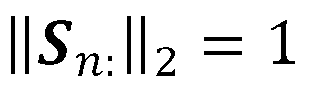
- the sample set further includes a calibration sample, the calibration sample includes all of the K types of components, and has a known composition, and the intensity correction is performed to convert the intensity distribution matrix into The method of [9], comprising normalizing.
- the intensity correction includes allocating at least a portion of the intensity distribution matrix by the product of the mass of the corresponding specimen in the specimen set and an environmental variable; The method according to [9], wherein the environmental variable is a variable representing the effect of the component on ionization efficiency during the observation.
- the environmental variable is a compound with a molecular weight of 50 to 1500 contained in the atmosphere at the time of the observation, or an organic low molecular weight compound with a molecular weight of 50 to 500 contained in each of the specimen sets in a predetermined amount.
- a composition estimation device for estimating the content ratio of the component in an estimation target specimen containing at least one component selected from K types of components, where K is an integer of 1 or more, Included in a sample set containing K or more training samples having different compositions, background samples not containing the above components, and the estimation target sample, which contain at least one component selected from the above K types of components
- a mass spectrometer that successively ionizes gas components generated by thermal desorption and/or thermal decomposition while heating each specimen, and continuously observes the mass spectrum, and information for processing the observed mass spectrum.
- the information processing device stores the mass spectrum obtained for each heating temperature in each row, obtains the two-dimensional mass spectrum for each specimen, and converts at least two of the two-dimensional mass spectra
- a data matrix creation unit that collectively converts the above into a data matrix
- NMF processing that performs non-negative matrix factorization of the data matrix and decomposes into the product of a normalized basis spectrum matrix and its intensity distribution matrix
- NMF A processing unit extracts a noise component included in the intensity distribution matrix by canonical correlation analysis between the base spectral matrix and the data matrix, corrects the intensity distribution matrix so as to reduce the influence of the noise component, and corrects the a correction processing unit that creates an intensity distribution matrix; divides the corrected intensity distribution matrix into submatrices corresponding to each of the specimen sets; a vector processing unit, an end member determination unit for setting a K-1 dimensional simplex containing all of the feature vectors, and determining K end members in the K-1 dimensional simplex; and the feature vector of the estimation target specimen,
- the sample for use comprises at least one of said endmembers.
- the end member determination unit determines the end members based on discriminant labels attached to the learning samples.
- the end member determination unit determines the end members by an algorithm that determines vertices so that the K-1 dimensional simplex has the minimum volume.
- the end member determination unit performs non-negative matrix factorization on the corrected intensity distribution matrix, and obtains a matrix representing the weight fraction of the K types of the components in the specimen, and the K types of individual components.
- the specimen set further includes a calibration specimen, the calibration specimen contains all of the K types of components, and has a known composition, and the intensity correction is performed to convert the intensity distribution matrix to The composition estimation device according to [17], including normalizing.
- the intensity correction includes assigning at least a portion of the intensity distribution matrix by the product of the mass of the corresponding analyte in the analyte set and an environmental variable;
- a mass spectrometer that sequentially ionizes gas components generated by thermal desorption and/or thermal decomposition while heating each sample contained in a sample set and continuously observes the mass spectrum, and the observed mass spectrum.
- a data matrix creation function that converts at least two or more of the above into a data matrix collectively, and NMF processing that decomposes the data matrix into a product of a normalized basis spectrum matrix and its intensity distribution matrix by non-negative matrix factorization extracting the noise component contained in the intensity distribution matrix by the NMF processing function and the canonical correlation analysis between the base spectrum matrix and the data matrix, and correcting the intensity distribution matrix so as to reduce the influence of the noise component.
- a correction processing function that creates a post-correction intensity distribution matrix by dividing the post-correction intensity distribution matrix into submatrices corresponding to each of the specimens, and using the submatrices as feature vectors, the specimens in the vector space and an end member determination function for setting a K-1 dimensional simplex containing all of the feature vectors and determining K endmembers in the K-1 dimensional simplex, Euclidean distances between the K end members and the feature vector of the estimation target specimen are calculated, and the content ratio of the component in the estimation target specimen is estimated from the ratio of the Euclidean distances.
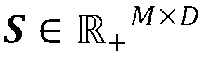
- the K is 3 or more, at least one of the feature vectors of the learning specimen is located in each of the regions outside the hypersphere inscribed in the K-1-dimensional simplex, or , the program, wherein the training sample comprises at least one of the endmembers.
- the method of the present invention heats each sample contained in a sample set, sequentially ionizes gas components generated by thermal desorption and / or thermal decomposition, and obtains a mass spectrum. Observing continuously, obtaining a two-dimensional mass spectrum for each specimen in which the obtained mass spectrum for each heating temperature is stored in each row, and normalizing the data matrix summarizing these by non-negative matrix factorization (NMF)
- NMF non-negative matrix factorization
- the noise component contained in the intensity distribution matrix is extracted and corrected by canonical correlation analysis, and the corrected intensity distribution matrix containing the feature vector of each specimen is obtained.
- One of the characteristic points is the subsequent quantitative calculation.
- the present method determines the mixture ratio (composition ) can be estimated.
- the composition of the sample can be estimated more accurately and easily.
- the endmembers can be determined from the label information, so the composition of the sample can be estimated more easily.
- the endmembers can be determined by vertex component analysis of the feature vector of the training specimen, and the composition of the specimen can be estimated. can.
- the composition of the sample can be determined by determining the end member by using an algorithm that determines the vertex so that the K-1 dimensional simplex has the minimum volume. can be estimated. It is excellent in that it does not require an end member as a training sample.
- the post-correction intensity distribution matrix is the post-intensity correction of the intensity distribution matrix, the accuracy of the estimation is further enhanced.
- the composition of the sample can be estimated with higher accuracy using a simpler procedure.
- the composition of the specimen can be estimated with high accuracy.
- a compound with a molecular weight of 50 to 1500 contained in a predetermined amount in the atmosphere at the time of observation, or an organic low molecule with a molecular weight of 50 to 500 contained in a predetermined amount in each sample of the sample set If it is the total value of the peaks of the mass spectrum of the compound, even if the sample set does not include the calibration sample, a simpler operation will yield a more accurate composition estimation result.
- FIG. 4 is a flow chart of a composition estimation method according to an embodiment of the present invention
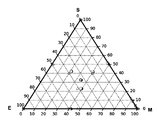
- FIG. 10 is an image diagram showing a K ⁇ 1 dimensional simplex (two-dimensional simplex, triangle) when K is 3
- 1 is a hardware configuration diagram of a composition estimation device according to an embodiment of the present invention
- FIG. 1 is a functional block diagram of a composition estimating device according to an embodiment of the present invention
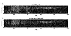
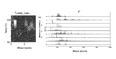
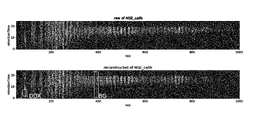
- FIG. 10 is a diagram showing the original spectrum (A) and the reconstructed spectrum (B) after processing for "MSE_calib"; Part C ⁇ (MSE_Calib) of the C matrix after NMF decomposition and S T after removing background and impurity spectra by CCA-Filter.
- FIG. 10 is a diagram showing the original spectrum (upper, raw of MSE_calib) for "MSE_calib" and the reconstructed spectrum after performing the above processing with the CCA-filter removed. It is a composition estimation result when correction by an environmental variable is not performed.
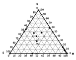
- FIG. 10 is an image diagram showing a K ⁇ 1 dimensional simplex (two-dimensional simplex, triangle) when K is 3; It is an explanatory diagram of the mechanism of the end member determination method in the second embodiment of the present invention.
- FIG. 11 is a diagram showing estimation results of Example 2;
- FIG. 11 is a diagram showing estimation results of Example 3;
- component means a substance that constitutes each sample, and estimation target samples, learning samples, and calibration samples mean mixtures made up of combinations of components.
- Presume target sample is a sample whose composition should be estimated, and both the number of components contained and the content of each component may be unknown.
- the "learning sample” means a sample necessary for determining K endmembers of the K-1 dimension simple substance described later, and these samples include at least one component selected from K components. contained, each with a different composition.
- the number of components contained is not particularly limited, and may be from 1 to K types.
- the learning sample may contain the same composition as the estimation target sample. That is, the estimation target sample and the learning sample may be the same, but the learning samples are different.
- End member means a vector corresponding to the vertex of a K-1 dimensional simplex, and this end member is a sample (learning sample or virtual sample) consisting of only one component of K types. Corresponds to the feature vector.
- a “background sample” means a sample that is different from the estimation target sample and the learning sample and that does not contain any of the above components.
- a “calibration sample” means a sample that is different from the estimation target sample, the learning sample, and the background sample, contains all K types of components, and has a clear composition.
- FIG. 1 is a flow chart of a composition estimation method (hereinafter also referred to as “this method”) according to an embodiment of the present invention.
- an estimation target specimen, K or more learning specimens with mutually different compositions, and background specimens are prepared (step S101).
- the sample set may further include a calibration sample.
- the estimated target sample contains at least one of the K types of components. If the analyte of interest contains one type of component, the purity of that component can be estimated by this method. In this case, the presumed target specimen includes the above-mentioned "ingredient" and other impurities.
- the putative target analyte is a mixture of components.
- the upper limit is not particularly limited.
- K is preferably 1000 or less.
- the number of learning samples is related to the number of components K, and must be K or more. If it is K or more, the number of learning samples is not particularly limited, but if it is more, the accuracy of determining the vertices of the K-1-dimensional simple substance described later tends to be higher, and as a result, more accurate composition estimation. Easy to get results.
- the ratio of the number of learning samples to the number of components K is 1 or more, preferably 2 or more, more preferably 3 or more, further preferably 5 or more, and 10 or more.
- the upper limit is not particularly limited, but generally 1000 or less is preferable.
- the learning samples differ in composition from each other.
- the composition is determined by the type and number of components contained and the content of each component.
- the same composition means that the type, number, and content of the contained components are the same, and if any one of them is different, it will be in a state of "different compositions.”
- the learning samples have different compositions
- other information that is, the types of components contained, the number of components, and the contents of each component, is used for estimating the composition of the estimation target sample.
- the composition of the training sample may be unknown.
- the difference between the estimation target sample and the learning sample is that the learning sample must have different compositions.
- the learning samples may include those having the same composition as the estimation target sample.
- the training sample may contain end members. That is, the learning sample may contain one type of component selected from K types of components (simple, pure). When the training sample contains end members, it is possible to more easily and accurately estimate the composition.
- the end-member learning sample may include a discriminant label. It is preferable that the training sample contains a discriminant label, because it makes it easier to determine the endmembers.
- each of the estimation target specimens is heated to sequentially ionize gases generated by thermal desorption and/or thermal decomposition to acquire a mass spectrum (step S102).
- the method of obtaining a mass spectrum is not particularly limited, a method of performing mass spectrometry on a sample under ambient conditions without pretreatment is preferred.
- a mass spectrometer called DART-MS, which combines an ion source called DART (Direct Analysis in Real Time) ion source and a mass spectrometer, is known.
- the mass spectrometer is not particularly limited, and is preferably capable of accurate mass spectrometry, and may be either a quadrupole type, a time-of-flight (TOF) type, or the like.
- each sample contained in the sample set is sequentially heated at a heating rate of 50 ° C./min, and heated to 50 to 550
- the mass spectrum obtained for each heating temperature is stored in each row to obtain a two-dimensional mass spectrum for each specimen, and at least two or more of these two-dimensional mass spectra are collectively converted into a data matrix (step S103 ).
- step S102 mass spectra are continuously acquired at predetermined temperature rise intervals. These mass spectra may be used to create a data matrix as they are, or may be averaged for each predetermined heating temperature range. The amount of data can be compressed by averaging the mass spectra for each predetermined heating temperature range into one line. Such a temperature rise range is, for example, about 10 to 30.degree.
- the peak intensity may be normalized.
- a method of normalization for example, a method of normalizing so that the sum of squares of peak intensities becomes 1 can be used.
- the number of two-dimensional mass spectra used to create the data matrix X is not particularly limited as long as it is two or more, it is preferable to use the two-dimensional mass spectra of all samples included in the sample set.
- part or all of the two-dimensional mass spectrum obtained by the measurement two or more times may be used to create the data matrix X. .
- NMF non-negative matrix factorization
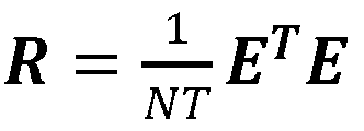
- the spectral data matrix is generally
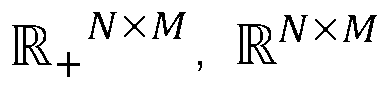
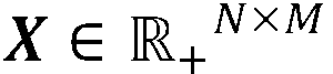
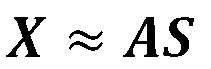
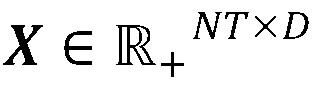
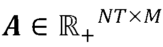
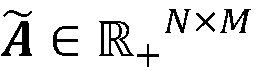
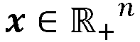
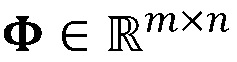
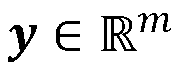
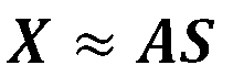
- the data matrix X is an N ⁇ M data matrix formed by stacking N spectra with M channels
- S is a base spectrum matrix
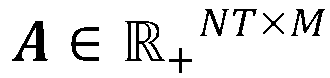
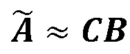
- C is its intensity distribution matrix. If the number of all elements included in the data set is K1, then C is an N ⁇ K1 matrix and S is an M ⁇ K1 matrix. Since the actual measurement contains noise,
- the NMF processing in this step is performed by alternately updating the column vectors of C and S according to Hierarchical alternating least square (HALS), which is easy to incorporate the constraints described below. is preferably solved as a convex optimization problem for each column of .
- HALS Hierarchical alternating least square
- a mass spectrometer generally has a resolution of about 0.1 to 0.001 m/z. Therefore, situations in which the m/z of different gas components match to the nearest decimal point and occupy the same channel are rare. Therefore, it is reasonable to assume some degree of orthogonality between the column vectors of the basis spectral matrix S.
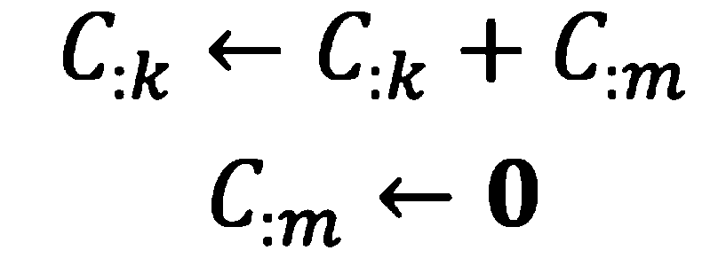
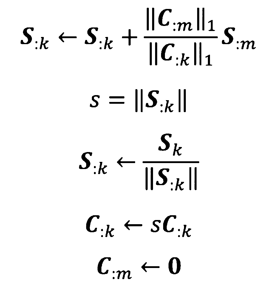
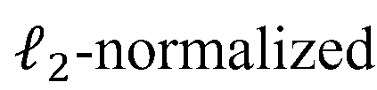
- Threshold is a hyperparameter given between 0.9 and 0.99. It is preferable to merge similar S in a similar manner, and also to superimpose the corresponding column vectors of S according to the weight of C, even when multiple column vectors of C are parallel. i.e.
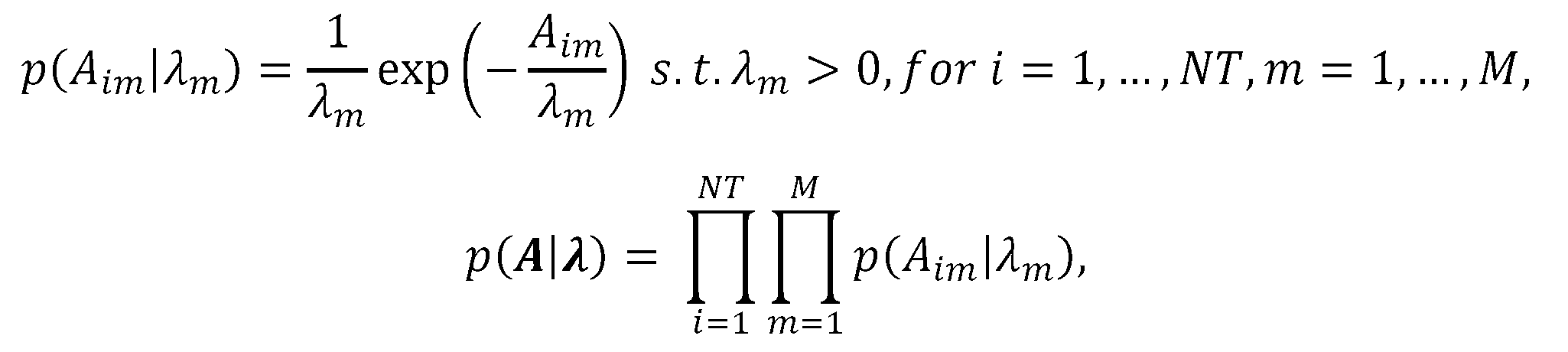
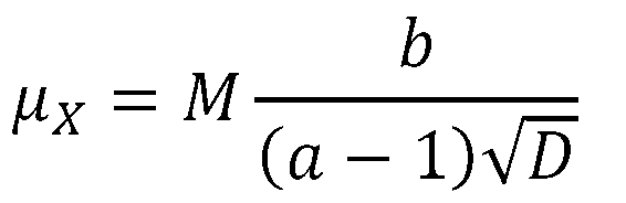
- the element ⁇ k of is a parameter following an inverse gamma distribution representing the importance of the component k in the data. Since we assumed a Gaussian distribution for the noise
- a is a hyperparameter such that a-1 is a very small positive number
- b is the average value ⁇ X of the data matrix.
- ⁇ k is the Lagrangian undetermined multiplier
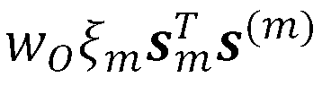
- the soft orthogonality condition can freely adjust the degree of orthogonality between complete orthogonality and no orthogonality constraint by multiplying ⁇ k by a hyperparameter w of [0, 1].
- the final update formula is
- the base spectrum matrix and the data matrix are subjected to canonical correlation analysis to obtain a corrected intensity distribution matrix (step S105).
- the noise component contained in the intensity distribution matrix is extracted by canonical correlation analysis between the base spectrum matrix and the data matrix, the intensity distribution matrix is corrected to reduce the influence of the noise component, and the corrected intensity distribution matrix is get
- NMF is a low-rank approximation of the data matrix, even if the component k does not actually exist in the i-th spectrum, if the approximation is better in the sense of least squares, then C ik >0 and In many cases such C ik is very small and often does not matter in NMF analysis.
- C jk >0 which is present in trace amounts in the j-th spectrum
- C ik >0 which is an NMF artifact
- substitute 0 for C ik which is a ghost peak
- Canonical Correlation Analysis is used to solve the above.
- This step is one of the features of this method, and the present inventors named this step Canonical Correlation Analysis (CCA) Filter.
- CCA Canonical Correlation Analysis
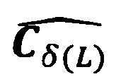
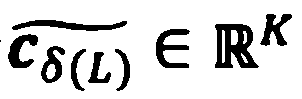
- the CCA filter scans sample-wise whether each component of the base spectrum S T output from NMF was actually included in the original data, and if no peak pattern similar to the original data is found, By erasing from the spectrum of that sample. If the spectrum generated from the L-th sample is stored in rows 1 to 1' of the data matrix X, the submatrix extracting that portion is written as X ⁇ (L) . , l'-2, l'-1 ⁇ .
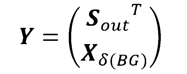
- CCA is conventionally known as a technique for examining the correlation between data of two systems, and is formulated as follows.
- a matrix of N p-dimensional vectors is
- a matrix consisting of N q-dimensional vector data is
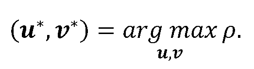
- the CCA problem setting is to project Y and Z onto a certain axis and find the solution (a T ,b T ) T that maximizes the correlation coefficient ⁇ .
- the noise that can be removed by the CCA filter includes, for example, (1) NMF artifacts (so-called false peaks), (2) peaks derived from trace chemical substances that slip into the surrounding environment of the device (background), (3) However, there are peaks (contamination) derived from substances that may distort the nature of the analysis if included in the analysis.
- Contaminants include, but are not limited to, solvents used in sample preparation and loading.
- This step may further include a step of intensity correction of the intensity distribution matrix.
- DART-MS primarily ionizes water and ammonia in the air with helium ions, which secondarily ionizes the sample. Therefore, the peak intensity may change depending on atmospheric conditions such as humidity. Also, the sample mass to be loaded is usually different for each sample, which also affects the peak intensity. Also, the ionization efficiency of each component contained in the sample is generally different, which also affects the peak intensity. By intensity correction of the intensity distribution matrix, the above effects can be reduced and more accurate quantification results can be obtained.
- the intensity correction can be performed by normalizing the intensity distribution matrix.
- Normalizing the intensity distribution matrix means normalizing the C matrix for each specimen, and more specifically means an operation of adding all elements to 1 for each specimen. If we divide the C matrix sample-wise and denote the C matrix derived from sample L as C ⁇ (L) ,
- the ionization efficiency differs for each compound, and the thermal decomposition efficiency also differs, and the amount of compound and the peak intensity are not proportional.
- the peak intensity ratio including the ionization efficiency of component k by NMF is already reflected in S :kT , and the intensity ratio between spectra is reflected in C :k . Thanks to this hierarchical data structure formed by NMF, more accurate quantitative compositional analysis is possible without obtaining unknown ionization efficiencies, as long as peak intensity ratios at the endmembers are taken into consideration.
- the specimen set does not include calibration specimens
- more accurate quantitative analysis is possible by assigning at least part (preferably all) of the intensity distribution matrix by the product of the mass of the corresponding specimen and the environmental variable.
- the environmental variable is a variable representing the influence of each component on the ionization efficiency during observation.
- a component with a high ionization efficiency has a high peak intensity
- a component with a low ionization efficiency has a low peak intensity.
- the peak intensity generally increases as the mass increases, and the peak intensity decreases as the mass decreases.
- the C matrix is corrected as follows so that the intensity information between samples held by the intensity distribution matrix can be used without normalizing the intensity distribution matrix.
- m L is the mass of sample L
- I L is the peak intensity of (poly)dimethylsiloxane generated from the oil pump attached to the DART-MS, observed in the entire temperature range at 610 m/z.
- IL reflects the standby state at the time of measurement, and there is a difference of about three times in peak intensity between rainy days and sunny days. corrected by this
- I L is 610 m/z derived from (poly)dimethylsiloxane, but is not limited to the above, and is derived from a compound with a molecular weight of 50 to 1500 contained in a predetermined amount in the atmosphere at the time of observation. and/or derived from an organic low-molecular-weight compound having a molecular weight of 50 to 500 contained in a predetermined amount in each of all samples.
- the corrected intensity distribution matrix is divided into submatrices corresponding to the respective specimens included in the specimen set, and each specimen is expressed in the vector space as a feature vector (step S106 ). Furthermore, a K-1 dimensional simplex containing all of these feature vectors (each corresponding to each specimen) is set, and K endmembers in the K-1 dimensional simplex are determined (step S107).
- the training specimen contains an end member and the training specimen has a discriminative label (a label for distinguishing that the training specimen is an "end member"), based on that label End members are determined.
- the training sample contains endmembers and the training sample is not labeled discriminatively, i.e. the training sample contains endmembers, but which training sample is the endmember If is unknown, the endmembers are determined by Vertex Component Analysis of the feature vector.
- the endmembers are determined by an algorithm that determines the vertices so that the K-1 dimensional simplex has the minimum volume. It should be noted that the fact that the K ⁇ 1 dimensional simplex has the minimum volume means the minimum area in the case of a two-dimensional simplex (triangle).
- At least one of the feature vectors of the training specimen is located in each of the regions outside the hypersphere inscribed in the K-1-dimensional simplex. (when K is 3 or more), the endmembers can be determined with high accuracy.
- FIG. 2 is an image diagram showing a K-1 dimensional simplex (2-dimensional simplex, triangle) when K is 3.
- the K-1 dimensional simplex 10 is a triangle whose vertices are the end members 13, 14 and 15 determined by the training specimens 16, 17 and 18.
- the algorithm for determining the vertices so that the K-1 dimensional simplex has the minimum volume is not particularly limited, and a known algorithm can be applied.
- Examples of such algorithms include the Minimum Volume Constraint-NMF method, the Minimum Distance Constraint-NMF method, the Simplex identification via split augmented Lagrangian method, and the Simplex volume minimization method.
- the Euclidean distance between the K endmembers and the feature vector of the sample to be estimated is calculated, and the content ratio of each component in the sample is estimated (step S108).
- the feature vector of the other training sample is K ⁇ It may be located in a region inside a hypersphere inscribed in a one-dimensional simplex.
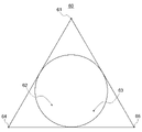
- FIG. 13 is an image diagram showing a K-1 dimensional simplex (two-dimensional simplex, triangle) when K is 3, as in FIG.
- a K-1 dimensional simplex 60 is a triangle whose vertices are end members 64 and 65 determined by a learning sample 61 as an end member, another learning sample 62 and a learning sample 63 .
- the difference from FIG. 2 is that the learning specimens 62 and 63 are located in the region inside the hypersphere inscribed in the K-1 dimensional simplex.
- the other learning samples may be located on a hypersphere inscribed in the K-1 dimensional simple substance, or may be located in the outer region. may be located. That is, in this case, the positions of other learning samples may be arbitrary.
- the other training sample contains 20% by mass or more of an endmember component (another endmember component) different from the endmember learning sample. It is preferably contained, and more preferably 40% by mass or more.
- step S107 in the already described first embodiment if the learning sample does not contain an end member, that is, there is no learning sample located at the K-1 dimensional simplex vertex Contains how the end members (vertices) of a case are determined.
- One of the features of the method according to this embodiment is that the determination of the endmembers is performed by non-negative matrix factorization of the matrix representing the fragment presence intensity for each sample, representing the weight fraction of the K types of components in the sample.
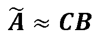
- the second NMF process decomposes into the product of the matrix and the matrix representing the fragment presence intensity for each single unit of the K kinds of components.
- FIG. 14 is a schematic diagram for explaining the mechanism.
- Each sample is a mixture of K types of components (hereinafter, described as a mixture of "polymers"), but what can actually be observed is the spectrum of M types of fragment gases generated by thermal decomposition of each polymer. is a suitable linear summation of S.
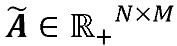
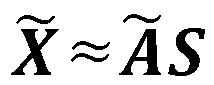
- the feature points according to the present embodiment have the coefficient matrix as given that, , and if it were possible to measure K polymer units, it would be If it is observed that and the idea that composition C can be obtained by performing a second NMF treatment.
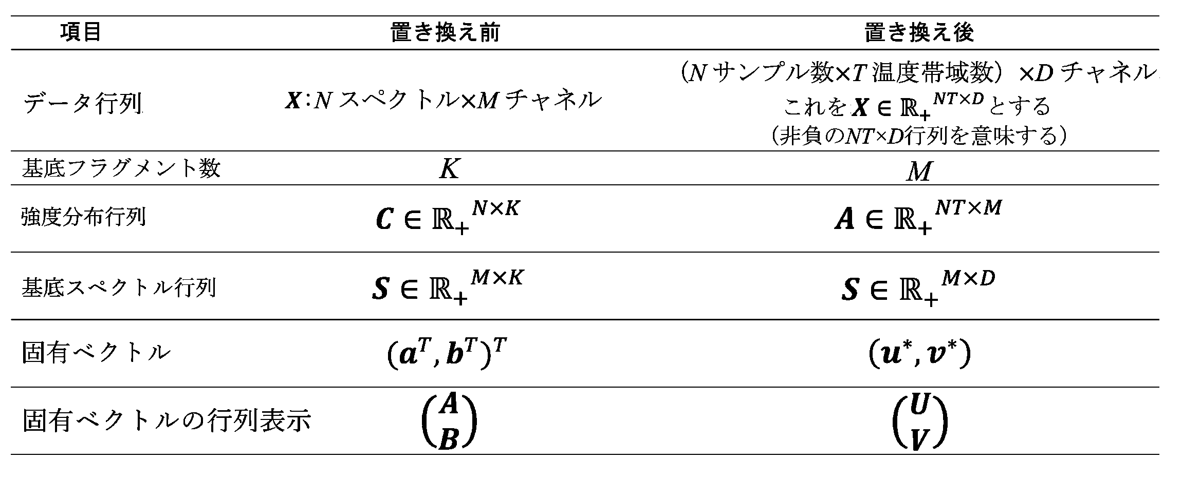
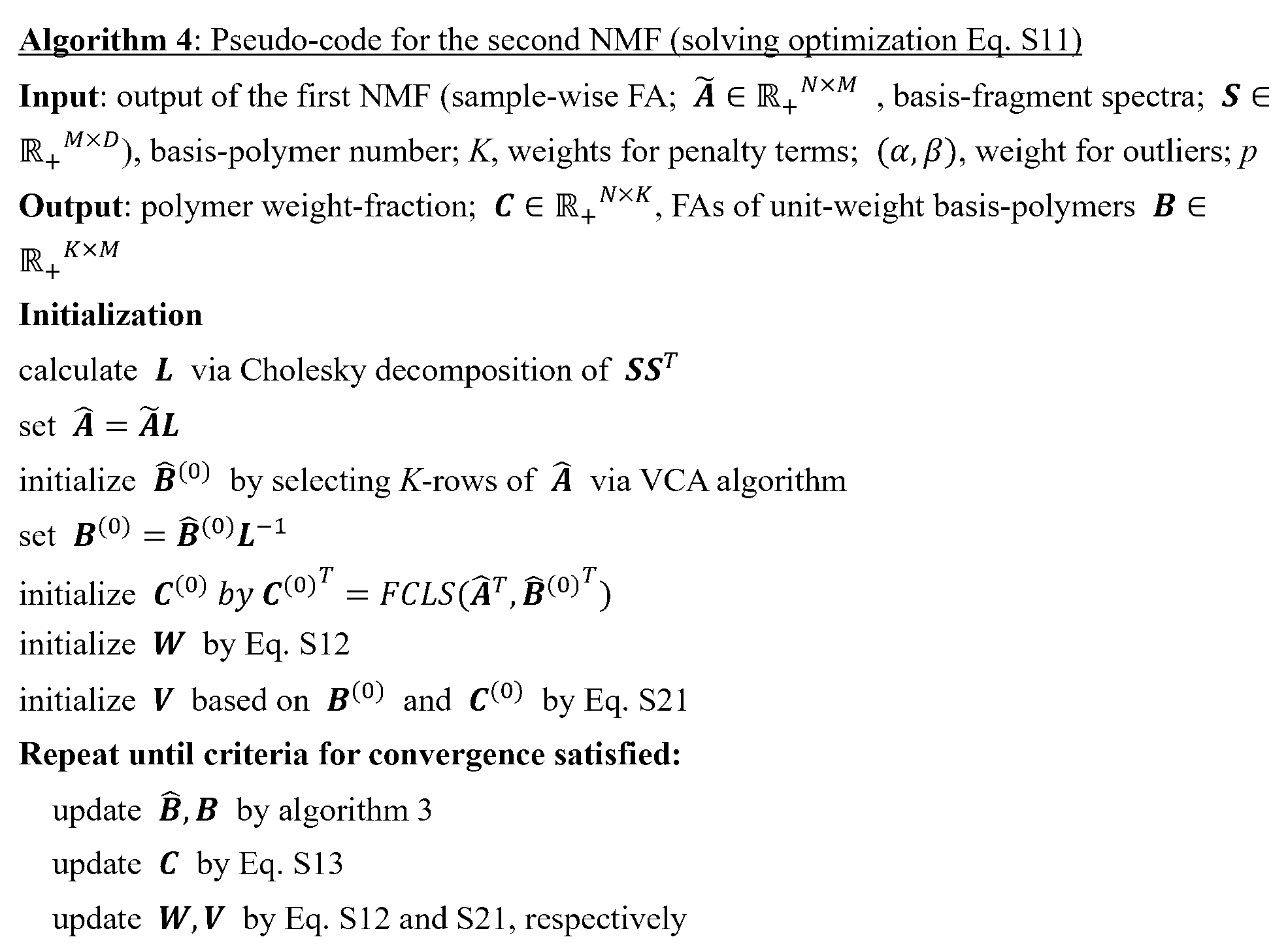
- step S104 (hereinafter also referred to as “first NMF processing”) and the NMF processing performed in determining the end members in step S107 (hereinafter “second NMF processing”) will be described. (also referred to as “processing”) will be described in detail. Note that, in principle, steps that are not described below are the same as the steps in the first embodiment.
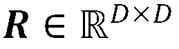
- N represents a non-negative or real N ⁇ M matrix.
- a queue against represent the n-th row vector, m-th column vector, and (n, m)-element, respectively.
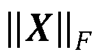
- X T is the transposed matrix of X, represents the Frobenius norm.
- Tr(X) represents a trace and diag(X) represents a diagonal matrix consisting of diagonal elements.
- 1 N and 11 N represent N-dimensional vectors or (N,N) matrices with all elements being 1's.
- I N represents an N-dimensional identity matrix.
- N the number of samples
- T the number of temperature band divisions
- D the number of channels
- M the number of base spectra
- the first NMF was developed to be well adapted to MS (Mass Spectrometry) data interpretation by adding the following three points to the ARD-SO-NMF proposed by Shiga et al.
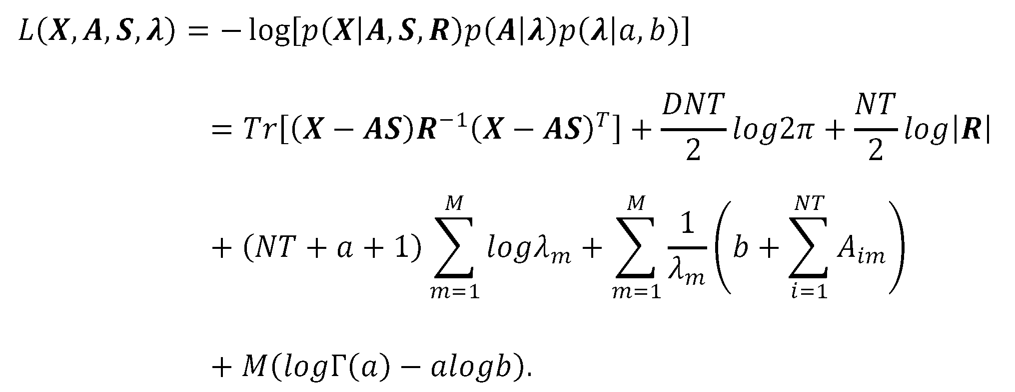
- the overall probabilistic model is can be written as where p(S) is and p( ⁇
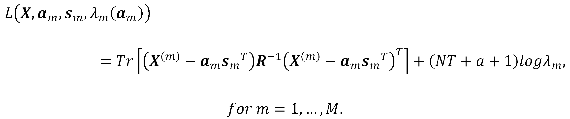
- a,b) is an inverse gamma distribution parameterized by (a,b), i.e. and a is a hyperparameter that adjusts sparsity, a 1+10 ⁇ 16 , b is empirically estimated from the expected value E(A im ) of A im , be associated with This is further expressed as E(X id ) and and approximating E(X id ) by the average ⁇ X of X, From b is is determined. So the negative log-likelihood function is can be written as Since this is a downward convex function with respect to ⁇ , i.e. , the update formula for ⁇ is obtained. Up to this point, the derivation of ARD-SO-NMF reported by Shiga et al. was completely followed.
- HALS hierarchical alternating least square
- the objective function to be minimized is and the gradient with respect to a m and s m is and if these are set to zero, the update formula is becomes. Since s m is normalized for each update, we omitted the constant factor.
- the non-negative constraint was satisfied by projecting into the non-negative quadrant at each update. Specifically, for example: can be projected by here means a vector with absolute values for each element.
- the first step consists of the M-spectrum Let the obtained S be a spectral set similar to S m: and dissimilar spectral sets is to divide into This split is is fulfilled.
- each spectral pair is as well as can be written as The similarity is evaluated by the correlation coefficient ⁇ , here, CCA's problem setting is can be written as the solution is given as a solution to the generalized eigenvalue problem, here is the eigenvector are arranged as column vectors in descending order of their eigenvalues. each eigenvalue is the correlation coefficient of y and z produced by linear combination with the corresponding (u * , v * ) as coefficients.
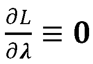
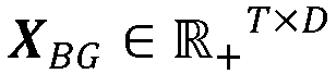
- the background component was removed from the system by deleting the corresponding column vector of A and row vector of S.
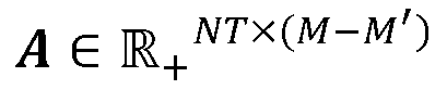
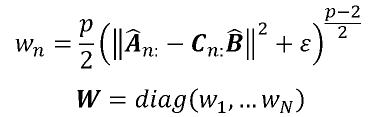
- the M'-component derived from the background has been removed (Hereinafter, MM' is replaced with M for simplicity, ) corrects the assigned intensity for the sample amount and the internal standard peak.
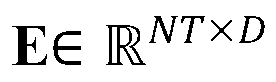
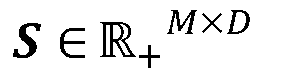
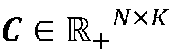
- the submatrix part A (n) of A for sample n was converted into a one-dimensional vector may be used as the input for the second NMF as the feature vector of sample n, but since the temperature distribution of M-fragments is unnecessary information in composition analysis, all temperature bands are summed for each sample to obtain M - represent the fragment abundance (FA) may be used as an input. here for simplicity We will do a second NMF on .
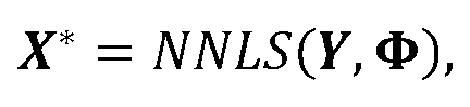
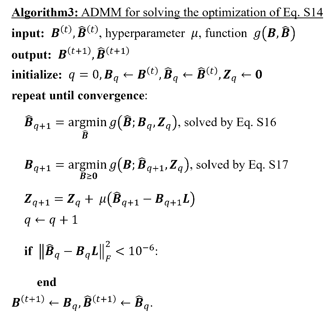
- NLS Non-negative least square
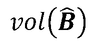
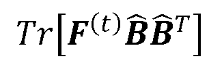
- the volume term of the simplex spanned by the row vector of Let the non-orthogonality terms between the row vectors of Assuming ⁇ >0 and ⁇ [0,1] as weights, by is sought.
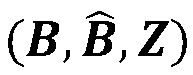
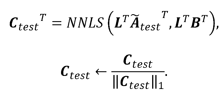
- test data is projected onto the hyperplane of S and B.
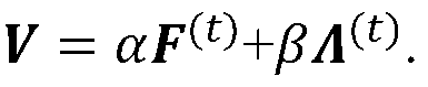
- S-hyperplane is obtained. i.e. Taking the sum over the temperature range, , by projection onto the B-hyperplane and normalization, is obtained. i.e.
- the dataset and hyperparameters are as follows.
- FIG. 3 is a hardware configuration diagram of the composition estimation device according to the embodiment of the present invention.
- the composition estimation device 30 includes a mass spectrometer 31 and an information processing device 33 , and the mass spectrometer 31 includes a decompression pump 32 .
- the information processing device 33 has a processor 34, a storage device 35, a display device 36, and an input device 37, and the mass spectrometer 31 and the information processing device 33 are configured to be able to exchange data with each other. .
- the processor 34 is, for example, a microprocessor, processor core, multiprocessor, ASIC (application-specific integrated circuit), FPGA (field programmable gate array), and GPGPU (general-purpose computing on graphics processing units).
- ASIC application-specific integrated circuit
- FPGA field programmable gate array
- GPGPU general-purpose computing on graphics processing units
- the storage device 35 has a function of temporarily and/or non-temporarily storing various programs and data, and provides a working area for the processor 34 .
- the storage device 35 is, for example, ROM (Read Only Memory), RAM (Random Access Memory), HDD (Hard Disk Drive), flash memory, SSD (Solid State Drive), and the like.
- the input device 37 can receive input of various types of information and input of instructions to the composition estimation device 30 .
- the input device 37 may be a keyboard, mouse, scanner, touch panel, or the like.
- the display device 36 can display the status of the composition estimation device 30, the progress of the analysis, the composition estimation results, and the like.
- the display device 36 may be a liquid crystal display, an organic EL (Electro Luminescence) display, or the like.
- the display device 36 may be configured integrally with the input device 37 .
- the display device 36 is a touch panel display, and the form which provides GUI(Graphical User Interface) is mentioned.
- the information processing device 33 which includes a processor 34, a storage device 35, an input device 37, and a display device 36 that can communicate data with each other via a data bus, is typically a computer.
- the mass spectrometer 31 is equipped with a vacuum pump 32 and is typically a mass spectrometer equipped with a DART ion source, a specimen heating device, and a time-of-flight mass spectrometer. Both the ion source and the mass spectrometer included in the mass spectrometer 31 are non-limiting examples, and the configuration of the mass spectrometer included in the present composition estimation apparatus is not limited to the above.
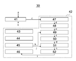
- FIG. 4 is a functional block diagram of the composition estimation device 30 according to the embodiment of the present invention.
- the composition estimating apparatus 30 has a mass spectrometer 41 that performs mass spectrometry on all specimens, and an information processor 42 that processes the mass spectrum obtained by the mass spectrometer 41 .
- the mass spectrometer 41 is configured including the mass spectrometer 31, and is a function realized by the mass spectrometer 31 being controlled by the control unit 43, which will be described later.
- the mass spectrometer 41 performs thermal desorption and/or thermal decomposition while heating the loaded specimen set (the specimen, the learning specimen, and the background specimen, symbol a in FIG. 4) to determine the gas components is ionized, mass spectroscopy is performed sequentially, and a mass spectrum is output (symbol c in FIG. 4).
- an environmental factor caused by the environment in which the mass spectrometer 31 is installed (symbol b in FIG. 4, for example, (poly)dimethylsiloxane generated from the decompression pump 32) is also loaded into the mass spectrometer 31 at the same time. Affects the spectrum.
- the control unit 43 is configured including the processor 34 .
- the control unit 43 implements each function of the composition estimation device 30 by controlling each unit.
- the storage unit 44 includes a storage device 35 .
- the storage unit 44 stores in advance a program for controlling each unit, and provides a temporary or non-temporary storage area for data input/output by each unit.
- the storage unit 44 is controlled by the control unit 43 and can read and write data.
- the input unit 45 includes an input device 37. Also, the output unit 46 is configured including the display device 36 . By controlling these, the control unit 43 receives input from the user of the composition estimation device 30, stores it in the storage unit 44, transmits information stored in the storage unit 44 to each unit, It can be displayed to the user of the composition estimation device 30 via the output unit 46 .
- the data matrix creation unit 47 is a function realized by executing the program stored in the storage unit 44 by the control unit 43 .
- the data matrix creation unit 47 creates a data matrix X from the two-dimensional mass spectrum in which the mass spectrum (symbol c in FIG. 4) acquired for each heating temperature by the mass analysis unit 41 is stored in each row, and performs NMF processing to be described later. It is passed to the unit 48 (symbol d in FIG. 4).
- the details of the data matrix X have already been explained.
- the NMF processing unit 48 is a function realized by executing the program stored in the storage unit 44 by the control unit 43 .
- the result is passed to the correction processing unit 49 (symbol e in FIG. 4).
- NMF non-negative matrix factorization
- the correction processing unit 49 is a function realized by executing the program stored in the storage unit 44 by the control unit 43 .
- the correction processing unit 49 has a function of correcting the intensity distribution matrix by canonical correlation analysis between the base spectrum matrix and the data matrix created by the NMF processing unit 48 to create a post-correction intensity distribution matrix.
- the created intensity distribution matrix after correction is passed to the vector processing unit 50 (symbol f in FIG. 4).
- the correction processing unit 49 may further perform the already-described intensity correction in addition to the above-described correction by the canonical correlation analysis.
- a calibration sample composition calibr sample composition
- it is passed to the correction processing unit 49 via the input unit 45 (symbol k in FIG. 4).
- CCA filter canonical correlation analysis
- the vector processing unit 50 is a function realized by executing a program stored in the storage unit 44 by the control unit 43 .
- the vector processing unit 50 divides the corrected intensity distribution matrix created by the correction processing unit 49 into sub-matrices corresponding to each of all the specimens, and expresses all the specimens in the vector space using these as feature vectors. This result is passed to the end member determination unit 51 (symbol g in FIG. 4).
- the end member determination unit 51 is a function realized by executing a program stored in the storage unit 44 by the control unit 43 .
- the end member determining unit 51 sets a K-1 dimensional simplex containing all the feature vectors generated by the vector processing unit 50, and determines K end members in the K-1 dimensional simplex. This result is passed to the content ratio calculator 52 (symbol h in FIG. 4).
- the learning sample contains an end member and has a discriminant label
- information on the discriminant label is passed from the input unit 45 to the end member determination unit 51 (symbol j in FIG. 4).
- the discrimination label is not essential for end member determination (processing by the end member determination unit 51).
- the content ratio calculation unit 52 is a function realized by executing the program stored in the storage unit 44 by the control unit 43 .
- the content ratio calculation unit 52 calculates Euclidean distances between the K endmembers determined by the endmember determination unit 51 and the feature vectors of the estimation target specimen created by the vector processing unit 50, respectively. From the ratio of the Euclidean distance between the endmember and the feature vector of the specimen, the content ratio of K components in the specimen to be estimated is estimated.
- the content ratio estimation result (indicated by symbol i in FIG. 4) is output from the output unit 46 . At this time, the result of estimating the composition of the learning sample may also be output.
- composition estimation apparatus even solid samples that are difficult to dissolve in solvents and difficult to perform conventional composition analysis can be subjected to analysis without special pretreatment, and accurate quantitative analysis results can be obtained. be done.
- This composition estimating apparatus can significantly reduce the time required to obtain results, particularly when applied to quality control of a sample that is a mixture of multiple components, investigation of causes of defects, and the like.
- composition analysis method will be described in detail based on examples.
- compositional analysis method of the present invention is not to be construed as being limited by the following specific examples.
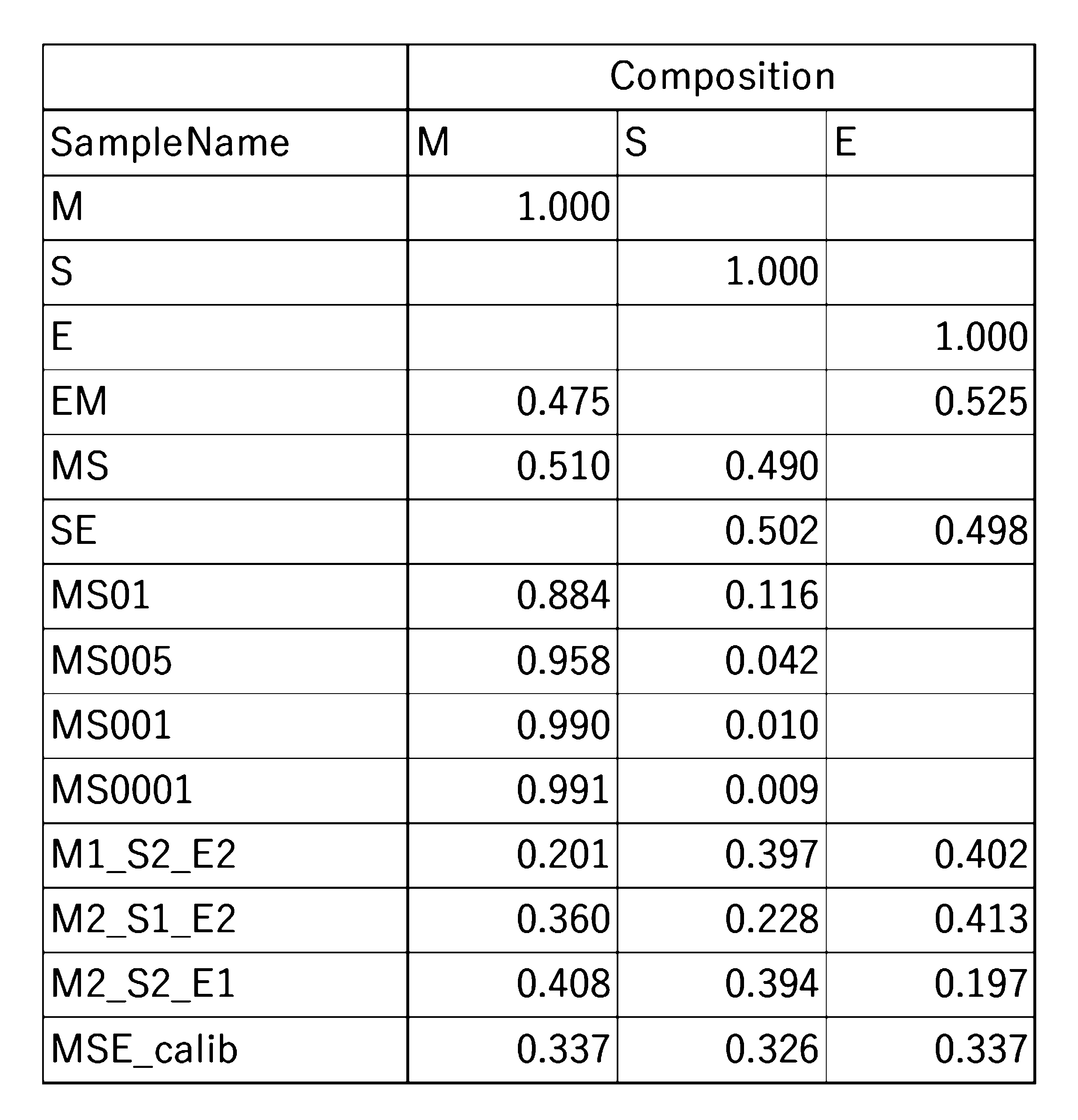
- Example 1 (Preparation of sample) Dioxane solution of three types of polymers: poly (methyl methacrylate), symbol “M”), polystyrene (symbol “S”), and polyethyl methacrylate (symbol “E”) (about 4% by mass, about 0.4 mg as polymer solid content) was cast on a sample pot and air-dried overnight to obtain a sample.
- Table 4 shows the composition of each sample. Mass spectrometry was performed using LCMS-2020 manufactured by SHIMADZU as a detector, a DART ion source manufactured by IonSense, and an ion rocket manufactured by Biochromato as a sample heating unit.
- FIG. 5 is a diagram showing the original spectrum (A) for "MSE_calib" and the reconstructed spectrum (B) after performing the above processing. It can be seen that both waveforms are similar. In other words, it was shown that the original spectral features were preserved by the above processing, making the data easier to use for compositional analysis.
- FIG. 6 shows a part C ⁇ (MSE_Calib) of the C matrix after NMF decomposition and S T after the background and impurity spectra are removed by the CCA-filter.
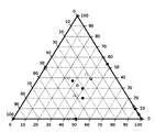
- Fig. 7 is the composition analysis result of the M, S, E ternary system.
- hollow circles and "Calibrated" in the legend indicate that MSE_calib is used as a calibration sample, that is, the composition information of MSE_calib is given as known, and the intensity distribution matrix is intensity-corrected. This is the composition estimation result of
- Non-calibrated is an environmental variable (i.e., 610 m / z: peak intensity of polydimethylsiloxane). It is the result of estimating the composition of a sample when the intensity distribution matrix is intensity-corrected.
- FIG. 8 shows composition estimation results when the orthogonal constraint (1) is canceled from the NMF conditions.
- the definition of each plot is the same as in FIG. From the results in FIG. 8, it can be seen that better estimation results are obtained when the NMF has orthogonality constraints.
- FIG. 9 shows composition estimation results when only merging S is canceled from the MNF optimization conditions.
- the definition of each plot is the same as in FIG. From the results of FIG. 9, it was found that better estimation results are obtained when the MNF optimization condition has merging S. Although the number of components can only be reduced to 36 by ARD, when the condition of Merging S is maintained, the composition can be estimated more accurately with the number of components of 9, which shows the importance of Merging S.
- FIG. 10 shows composition estimation results (comparative example) when the CCA-filter is canceled.
- the definition of each plot is the same as in FIG. In FIG. 10, the calculation result is that the sample "SE" contains about 1% of M even though the content of M is 0%. If 0% is estimated to be 1%, the estimation accuracy is not even several percent, which is not practical.
- FIG. 11 shows the original spectrum of “MSE_calib” (upper, raw of MSE_calib) and the reconstructed spectrum (lower, reconstructed of MSE_calib) after the above processing with the CCA-filter removed. be. From this result, it was found that when the CCA-filter was canceled, neither DOX nor BG noise (see description of FIG. 5) could be removed.
- Fig. 12 shows the composition estimation results when correction by environmental variables is not performed.
- "Non-calibrated" represented by solid circles deviates greatly from Known, and it was found that the estimation results obtained are more accurate by correction using environmental variables.
- Example 2 (Estimation based on samples not containing endmembers)
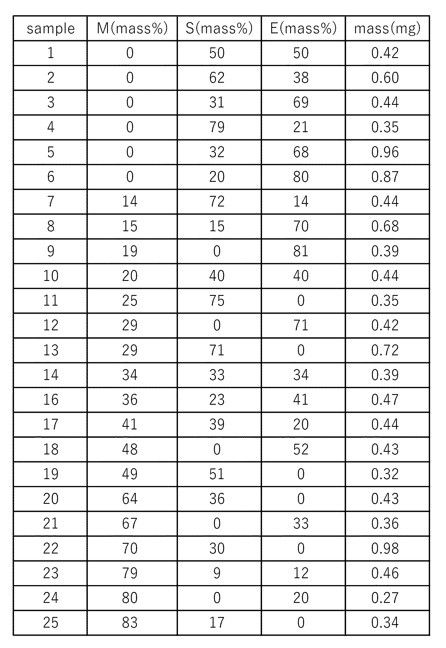
- the samples described in Table 5 were prepared and the same test as in Example 1 was performed.
- the symbols "M”, "S” and “E” mean the same as in Table 4 (Example 1).
- each sample is adjusted so that the weight fraction of a single component (polymer) does not exceed 80%.
- a two-dimensional mass spectrum was obtained for the specimen by the same method as in Example 1, and converted into a data matrix.
- the first NMF processing already described, i.e. carried out. Note that estimation of the variance-covariance matrix of noise can be calculated using only X, so it is performed inside the module in the first NMF processing.
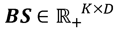
- FIG. 15 illustrates C and BS as a result.
- the composition estimated by this method is indicated by a circle, and the composition of the sample used (correct composition) is indicated by an asterisk. Both show good agreement.
- the absence of plots at the vertices of C also indicates that the samples used did not contain endmembers, ie pure polymers of E, S and M.
- BS in the figure shows the spectrum of the E, M, S pure polymer obtained by estimation and the spectrum of E, M, S actually measured, but there is no difference between the two, and the absolute intensity It was confirmed that it was well estimated, including
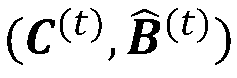
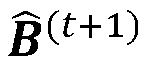
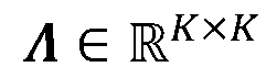
- the pure polymer spectra of E, M, S and the composition of the mixture can be accurately estimated as shown in FIG. 15 BS. rice field. If there is test data, X test is continuously projected onto S and B to obtain C test .
- Example 3 (Estimation from a specimen containing one endmember) Next, if one of the (training) specimens contains an endmember, the component content in the other specimen is arbitrary (it does not have to be the area outside the inscribed circle of the K ⁇ 1 dimensional simplex). We verified that.
- Composition estimation was performed in the same manner as in Example 2, except that among the samples listed in Table 5, samples containing 40% by mass or more of S were excluded and M pure polymer was added as a sample.
- FIG. 16 shows the results.
- the solid circle points represent the estimation results of the sample used for estimating B and S, and the asterisks are the actual compositions. From this result, it was confirmed that S can be estimated with high accuracy, although there were no specimens outside the inscribed circle (hollow circles are specimens that were not used for estimation).
- the non-orthogonality term is considered to be due to the incorporation of as a penalty term.
- fragments of the material are directly pyrolyzed in the atmosphere without pretreatment, the resulting gas is analyzed by DART-MS, and unsupervised learning of the spectrum is performed to obtain a pure endmember spectrum of each component. was estimated, and a method was developed to represent the spectrum of the sample by linear summation of the sum. This allows the identification and quantification of the components of even materials of complex composition without the need for separation.
- each peak intensity of the endmember spectrum can be estimated as an absolute intensity instead of a normalized relative value. It can be obtained as a ratio.
- the present invention which breaks down the sample into components and finds the content ratio, can be a useful tool in material development, such as identifying key components that are factors in demonstrating the performance of materials. Furthermore, it is expected to have a wide range of applications, such as quality control such as content inspection of degraded components, legal compliance inspection such as hazardous material content, and inspection for detecting infringement of rights. Furthermore, it is expected that technologies such as deterioration and lifespan prediction of resins, detection of minute impurity components in resins and organic materials, quantitative analysis of smell and taste, traceability of food products, and tags to prevent falsification of origin can be expected to accelerate.
- Plastics Europe proposed to the European Commission that plastic containers and packaging should contain 30% recycled plastic by 2030, promoting the use of recycled materials.
- the present invention is expected to be applied to quality control, legal compliance inspection, etc., as a technique capable of accurately measuring the ratio of virgin agent and recycled material.
Landscapes
- Chemical & Material Sciences (AREA)
- Analytical Chemistry (AREA)
- Bioinformatics & Cheminformatics (AREA)
- Crystallography & Structural Chemistry (AREA)
- Life Sciences & Earth Sciences (AREA)
- Engineering & Computer Science (AREA)
- Physics & Mathematics (AREA)
- Bioinformatics & Computational Biology (AREA)
- Computing Systems (AREA)
- Theoretical Computer Science (AREA)
- Spectroscopy & Molecular Physics (AREA)
- Other Investigation Or Analysis Of Materials By Electrical Means (AREA)
- Medical Treatment And Welfare Office Work (AREA)
Abstract
Description
また、本発明は、組成推定装置、及び、プログラムを提供することも課題とする。
[2] 上記Kが2以上の整数であり、上記推定対象検体が、上記成分の混合物である、[1]に記載の方法。
[3] 上記学習用検体が、上記エンドメンバーを含む、[1]又は[2]に記載の方法。
[4] 上記エンドメンバーの決定が、上記学習用検体に付された判別ラベルに基づき行われる、[3]に記載の方法。
[5] 上記エンドメンバーの決定が、上記学習用検体の上記特徴ベクトルの頂点成分分析によって行われる、[3]に記載の方法。
[6] 上記エンドメンバーの決定が、上記K-1次元単体が最小体積となるように頂点を定めるアルゴリズムによって実施される、[1]に記載の方法。
[7] 上記エンドメンバーの決定が、上記補正後強度分布行列を非負値行列因子分解し、上記検体中のK種類の上記成分の重量分率を表す行列と、K種類の個別の上記成分ごとのフラグメント存在強度を表す行列との積に分解する第2のNMF処理により行われる、[6]に記載の方法。
[8] 上記学習用検体が、上記エンドメンバーを含まない、[6]又は[7]に記載の方法。
[9] 上記補正後強度分布行列を得ることは、更に、上記強度分布行列の強度補正を行うことを含む、[1]~[8]のいずれかに記載の方法。
[10] 上記検体セットが、更に、キャリブレーション検体を含み、上記キャリブレーション検体は、上記K種類の成分を全て含み、かつ、その組成が既知であり、上記強度補正は、上記強度分布行列を規格化することを含む、[9]に記載の方法。
[11] 上記強度補正は、上記強度分布行列の少なくとも一部を、上記検体セットのうち対応する上記検体の質量と環境変数の積で割り付けることを含み、
上記環境変数は、上記観測の際における上記成分のイオン化効率への影響を表す変数である、[9]に記載の方法。
[12] 上記環境変数が、上記観測の際に、雰囲気中に所定量含まれる分子量50~1500の化合物、又は、上記検体セットのそれぞれに所定量含まれる分子量50~500の有機低分子化合物のマススペクトルのピークの合計値である、[11]に記載の方法。
[13] Kを1以上の整数としたとき、K種類の成分から選択される少なくとも1種の上記成分を含む推定対象検体における、上記成分の含有量比を推定する組成推定装置であって、上記K種類の成分から選択される少なくとも1種の成分を含み、互いに組成の異なるK個以上の学習用検体、上記成分を含まないバックグラウンド検体、及び、上記推定対象検体を含む検体セットに含まれるそれぞれの検体を加熱しながら、熱脱着、及び/又は、熱分解によって生ずるガス成分を順次イオン化し、マススペクトルを連続的に観測する質量分析装置と、上記観測されたマススペクトルを処理する情報処理装置と、を備え、上記情報処理装置は、加熱温度ごとに得られた上記マススペクトルを各行に格納し、上記検体ごとの二次元マススペクトルを得て、上記二次元マススペクトルの少なくとも2つ以上をまとめてデータ行列に変換する、データ行列作成部と、上記データ行列を非負値行列因子分解し、規格化された基底スペクトル行列とその強度分布行列の積に分解するNMF処理を行う、NMF処理部と、上記基底スペクトル行列と上記データ行列との正準相関分析によって強度分布行列に含まれるノイズ成分を抽出し、上記ノイズ成分の影響を減ずるよう上記強度分布行列を補正して、補正後強度分布行列を作成する、補正処理部と、上記補正後強度分布行列を上記検体セットのそれぞれに対応する小行列に分割し、上記小行列を特徴ベクトルとして、ベクトル空間内で上記検体のそれぞれを表現する、ベクトル処理部と、上記特徴ベクトルの全てを内包するK-1次元単体を設定し、上記K-1次元単体におけるK個のエンドメンバーを決定する、エンドメンバー決定部と、上記K個のエンドメンバーと、上記推定対象検体の特徴ベクトルとの、ユークリッド距離をそれぞれ計算し、上記ユークリッド距離の比により、上記推定対象検体中の上記成分の含有量比を推定する、含有量比計算部と、を含み、上記Kが3以上の場合、上記K-1次元単体に内接する超球体の外側の領域のそれぞれに、上記学習用検体の特徴ベクトルの少なくとも1つが位置する、又は、上記学習用検体が上記エンドメンバーの少なくとも1つを含む、組成推定装置。
[14] 上記エンドメンバー決定部は、上記学習用検体に付された判別ラベルに基づいて上記エンドメンバーを決定する、[13]に記載の組成推定装置。
[15] 上記エンドメンバー決定部は、上記K-1次元単体が最小体積となるように頂点を定めるアルゴリズムによって上記エンドメンバーを決定する、[13]に記載の組成推定装置。
[16] 上記エンドメンバー決定部は、上記補正後強度分布行列を非負値行列因子分解し、上記検体中のK種類の上記成分の重量分率を表す行列と、K種類の個別の上記成分ごとのフラグメント存在強度を表す行列との積に分解する第2のNMF処理により上記エンドメンバーを決定する、[15]に記載の組成推定装置。
[17] 上記補正処理部は更に、上記強度分布行列の強度補正を行う、[15]に記載の組成推定装置。
[18] 上記検体セットが、更に、キャリブレーション検体を含み、上記キャリブレーション検体が、上記K種類の成分を全て含み、かつ、その組成が既知であり、上記強度補正が、上記強度分布行列を規格化することを含む、[17]に記載の組成推定装置。
[19] 上記強度補正は、上記強度分布行列の少なくとも一部を、上記検体セットのうち対応する上記検体の質量と環境変数の積で割り付けることを含み、
上記環境変数は、上記観測の際における上記成分のイオン化効率への影響を表す変数である、[17]に記載の組成推定装置。
[20] 上記質量分析装置は減圧ポンプを更に備え、上記環境変数が、上記減圧ポンプの稼働によって生ずる物質のマススペクトルのピークの合計値である、[19]に記載の組成推定装置。
[21] Kを1以上の整数としたとき、K種類の成分から選択される少なくとも1種の上記成分を含む推定対象検体における、上記成分の含有量比を推定する組成推定装置において用いられるプログラムであって、上記K種類の成分から選択される少なくとも1種の成分を含み、互いに組成の異なるK個以上の学習用検体、上記成分を含まないバックグラウンド検体、及び、上記推定対象検体を含む検体セットに含まれるそれぞれの検体を加熱しながら、熱脱着、及び/又は、熱分解によって生ずるガス成分を順次イオン化し、マススペクトルを連続的に観測する質量分析装置と、上記観測されたマススペクトルを処理する情報処理装置と、を備え、上記質量分析装置によって、加熱温度ごとに取得された上記マススペクトルを各行に格納し、上記検体ごとの二次元マススペクトルを得て、上記二次元マススペクトルの少なくとも2つ以上をまとめてデータ行列に変換する、データ行列作成機能と、上記データ行列を非負値行列因子分解し、規格化された基底スペクトル行列とその強度分布行列の積に分解するNMF処理を行う、NMF処理機能と、上記基底スペクトル行列と上記データ行列との正準相関分析によって強度分布行列に含まれるノイズ成分を抽出し、上記ノイズ成分の影響を減ずるよう上記強度分布行列を補正して、補正後強度分布行列を作成する、補正処理機能と、上記補正後強度分布行列を上記検体のそれぞれに対応する小行列に分割し、上記小行列を特徴ベクトルとして、ベクトル空間内で上記検体のそれぞれを表現する、ベクトル処理機能と、上記特徴ベクトルの全てを内包するK-1次元単体を設定し、上記K-1次元単体におけるK個のエンドメンバーを決定する、エンドメンバー決定機能と、上記K個のエンドメンバーと、上記推定対象検体の特徴ベクトルとの、ユークリッド距離をそれぞれ計算し、上記ユークリッド距離の比により、上記推定対象検体中の上記成分の含有量比を推定する、含有量比計算機能と、を含み、上記Kが3以上の場合、上記K-1次元単体に内接する超球体の外側の領域のそれぞれに、上記学習用検体の特徴ベクトルの少なくとも1つが位置する、又は、上記学習用検体が上記エンドメンバーの少なくとも1つを含む、プログラム。
以下に記載する構成要件の説明は、本発明の代表的な実施形態に基づいてなされることがあるが、本発明はそのような実施形態に制限されるものではない。
なお、本明細書において、「~」を用いて表される数値範囲は、「~」の前後に記載される数値を下限値及び上限値として含む範囲を意味する。
本明細書において使用される用語について説明する。なお、以下に説明のない用語については、当業者の間で普通に理解される意味で使用される。
図1は、本発明の実施形態に係る組成推定方法(以下、「本方法」ともいう。)のフローチャートである。
なお、学習用検体の個数は成分数Kに関係して、K個以上である必要がある。K個以上であれば、学習用検体の数としては特に制限されないが、より多い場合、後述するK-1次元単体の頂点の決定の精度がより高くなりやすく、結果として、より正確な組成推定結果が得られやすい。
すなわち、成分数Kに対する学習用検体の数の比(学習用検体の数/成分数)は、1以上であり、2以上が好ましく、3以上がより好ましく、5以上が更に好ましく、10以上が特に好ましい。一方、上限値は特に制限されないが、一般に、1000以下が好ましい。
推定対象検体と学習用検体との相違点は、学習用検体はそれぞれ組成が異なることが必要である点である。なお、学習用検体は、推定対象検体と組成が同一のものを含んでいてもよい。
質量分析計としては特に制限されず、精密質量分析が可能なものが好ましく、四重極型、及び、飛行時間(TOF)型等のいずれでもよい。
このマススペクトルが各行に格納され、加熱温度が各列に格納されると、検体ごとの二次元マススペクトルが得られる。
データ行列Xの作成に用いられる二次元マススペクトルの個数は2つ以上であれば特に制限されないが、検体セットに含まれる全検体の二次元マススペクトルが用いられることが好ましい。
なお、1つの検体について2回以上、測定が行われる場合には、2回以上の測定で得られた二次元マススペクトルの一部、又は、全てがデータ行列Xの作成に用いられてもよい。


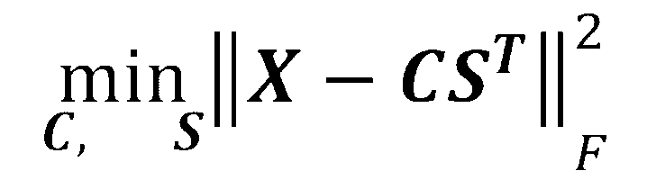




本ステップにおけるNMF処理は、以下に述べる制約を組み込みやすいHierarchical alternating least square (HALS)により、C、Sの列ベクトルワイズに交互に更新していくことで、上記式(数7)をC、Sの各列についての凸最適化問題として解くことが好ましい。
質量分析計は、一般に0.1~0.001m/z程度の分解能を有する。したがって、異なるガス成分のm/zが小数点以下まで一致し、同一のチャネルを占めるという状況は稀にしか生じない。したがって、基底スペクトル行列Sの列ベクトル間にはある程度の直交性を仮定するのが妥当である。
CとSの更新途中で、ほとんど同じ基底スペクトルが複数得られた場合は一つのスペクトルにまとめることで正しい成分数nを得ることができる。EALSのスペクトライメージをNMFに適用すると、Sのk番目の列ベクトルをS:kと書いて、ST :kS:m>thresholdなるk<mが存在するときに、

上記によって得られる更新式について説明する。
モデルの全同時分布は



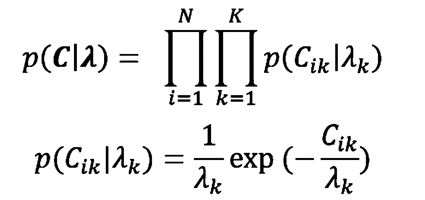

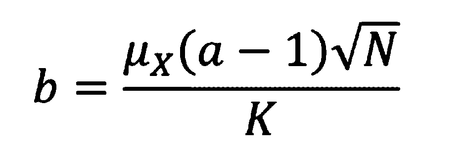
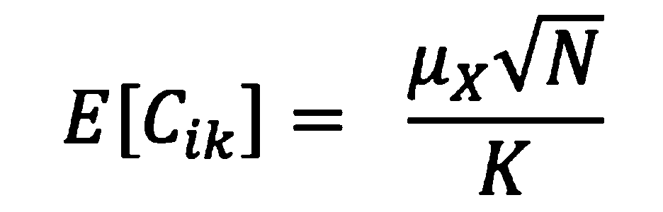


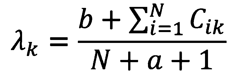
次に、Sの更新式について説明する。まず、負対数尤度関数からS:kに関連する項J(S:k)のみを取り出すことを考える。Xに対するk成分の寄与、




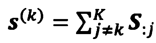


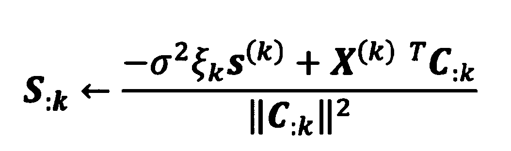
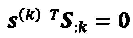
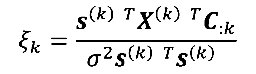
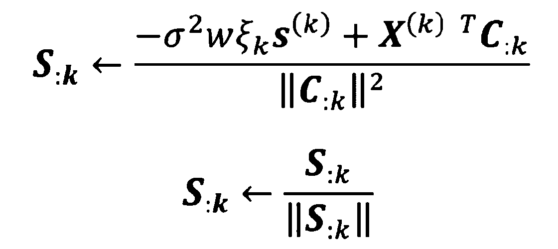
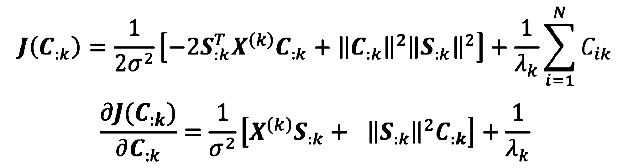

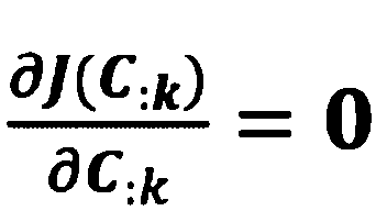
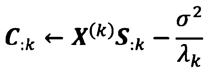
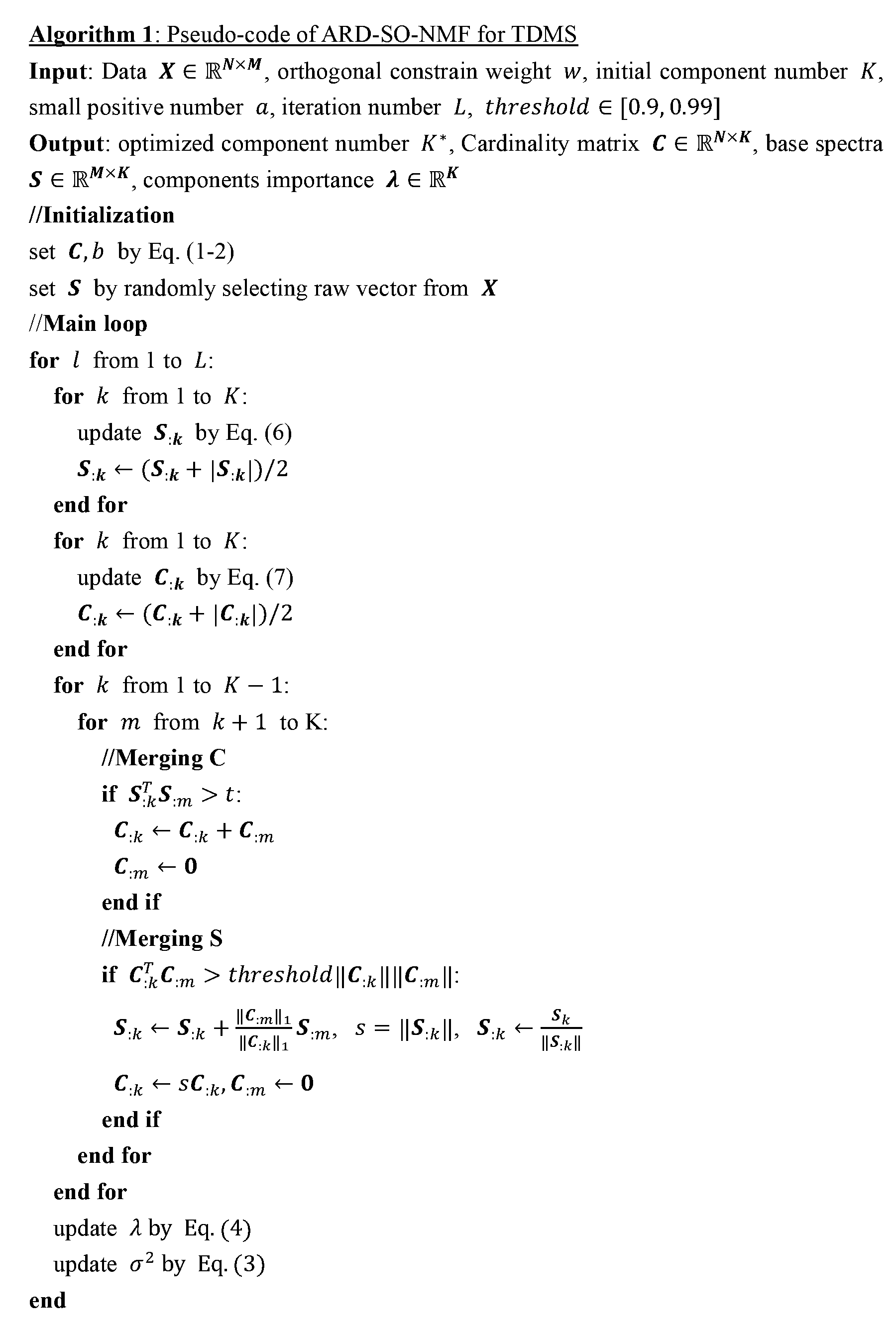
具体的には、基底スペクトル行列とデータ行列との正準相関分析によって強度分布行列に含まれるノイズ成分を抽出し、ノイズ成分の影響を減ずるよう強度分布行列を補正して、補正後強度分布行列を得る。
N個のp次元ベクトルからなる行列を


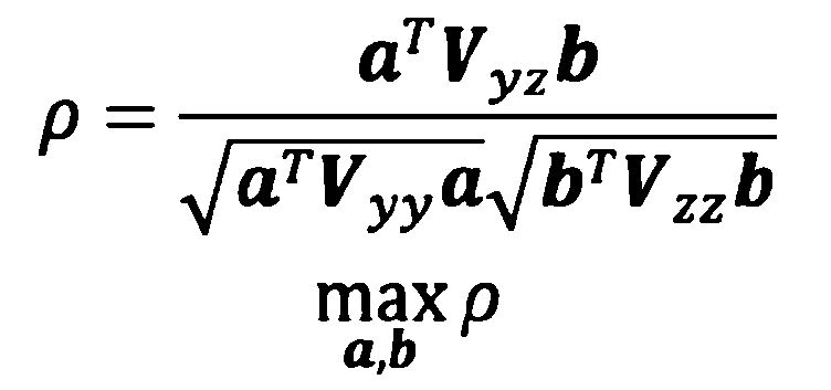


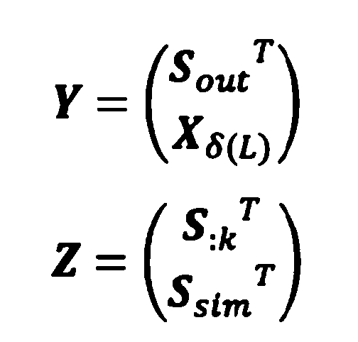
ここで、t1、t2はハイパーパラメータで、NMFのフィッティング精度、すなわちNMFハイパーパラメータであるthresholdの影響を強く受けるので、慎重に吟味する必要がある。経験的にt1=0.9threshold,t2∈[0.1,0.3]程度がよい結果を与える。
強度分布行列の強度補正によれば、上記の影響を減じて、より正確な定量結果を得ることができる。
C行列をサンプルワイズに分割し、サンプルLに由来するC行列をCδ(L)とかくと、





一つのキャリブレーション検体は必ず一つ以上の熱分解サンプルを与えるので、熱分解後の成分数はPは列フルランクな縦長の行列である。したがって一般的には解は不能で、最小二乗の意味での近似解は二次計画法で解くことができる。
しかし、NMFによって成分kのイオン化効率を含めたピーク強度比はS:k Tの中にすでに反映されており、スペクトル間の強度比はC:kに反映されている。
このNMFによって形成された階層的データ構造のおかげで、エンドメンバーにおけるピーク強度比さえ考慮にいれれば、未知のイオン化効率を求めなくても、より正確な定量的な組成分析が可能になる。
ここで、環境変数とは、観測の際における各成分のイオン化効率への影響を表す変数である。
また、検体の質量についても、これが大きくなれば、一般的にピーク強度は大きく成り、小さく成れば、ピーク強度は小さくなる。




さらに、これらの特徴ベクトル(それぞれ各検体に対応する)の全てを内包するK-1次元単体を設定し、K-1次元単体におけるK個のエンドメンバーを決定する(ステップS107)。
なお、上記はRobust Volume Minimization-Based Matrix Factorization for Remote Sensing and Document Clustering, IEEE TRANSACTIONS ON SIGNAL PROCESSING,VOL. 64,NO. 23,DECEMBER 1,2016をベースに考案された。
なかでも、より優れた本発明の効果が得られる点では、他の学習用検体は、エンドメンバーである学習用検体とは異なるエンドメンバーの成分(他のエンドメンバーの成分)を20質量%以上含むことが好ましく、40質量%以上含むことがより好ましい。
本方法の第2実施形態は、すでに説明した第1実施形態におけるステップS107において、学習用検体がエンドメンバーを含まない場合、すなわち、K-1次元単体頂点に位置する学習用検体が1つもない場合のエンドメンバー(頂点)の決定方法を含む。
各検体は、K種類の成分の混合物(以下では、「ポリマー」の混合物として説明する)であるが、実際に観測できるのは、各ポリマーが熱分解して生じたM種類のフラグメントガスのスペクトルSの適当な線形和である。


以下では、図1のフローにおける、ステップS104のNMF処理(以下、「1回目のNMF処理」ともいう。)と、ステップS107におけるエンドメンバーの決定において実施されるNMF処理(以下「2回目のNMF処理」ともいう。)の違い等について詳述する。なお、以下に説明のないステップ等については、原則として、第1実施形態における各ステップと同様である。
ある行列





全体の確率モデルとしては、





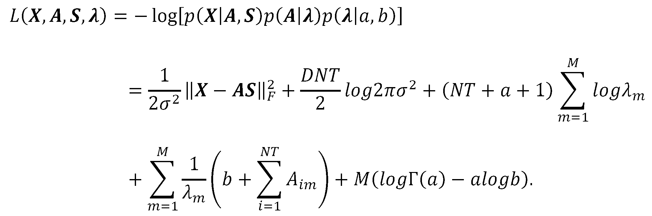





となる。λについての更新式Eq.S3を代入し、定数項を落として簡略化すると、




である。これによりL(X,A,S,λ)は成分mごとに分離して書けて、
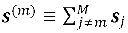

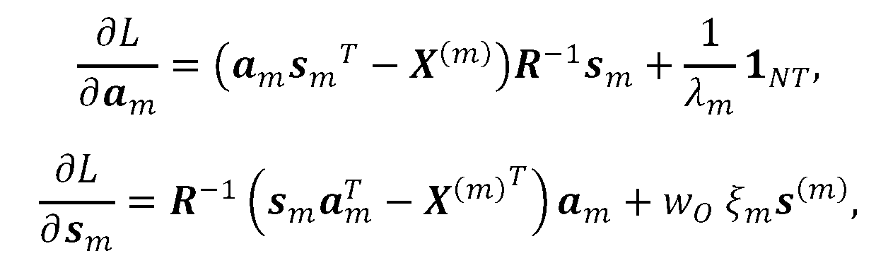

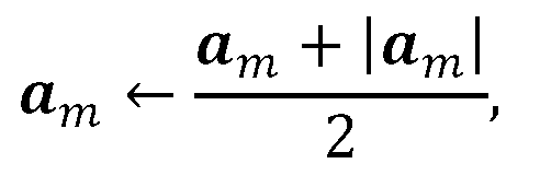

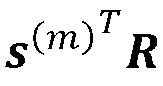
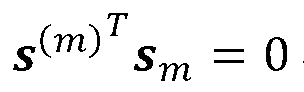
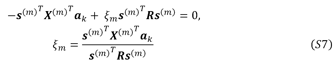
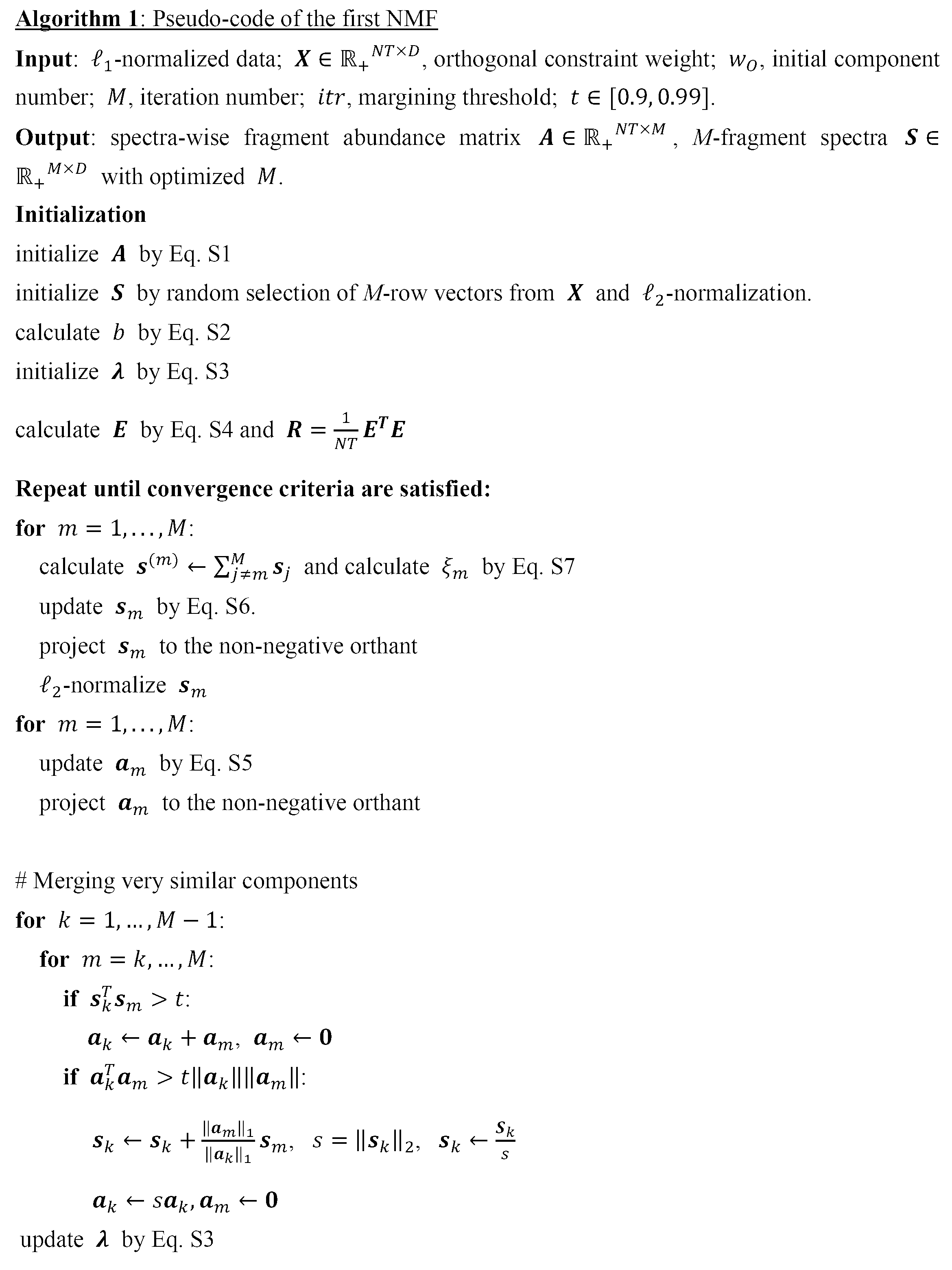
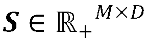



CCA-filterを用いるためには、バックグラウンドスペクトル
最初のステップは、M-スペクトルからなる
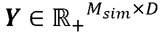
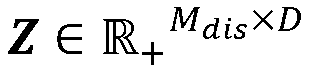

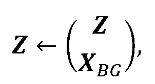
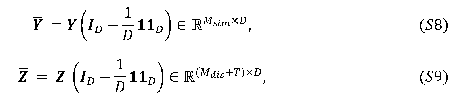


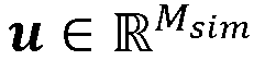
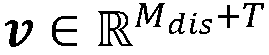
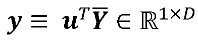
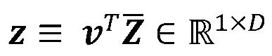


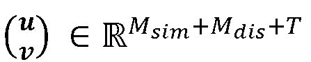

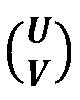

各固有値


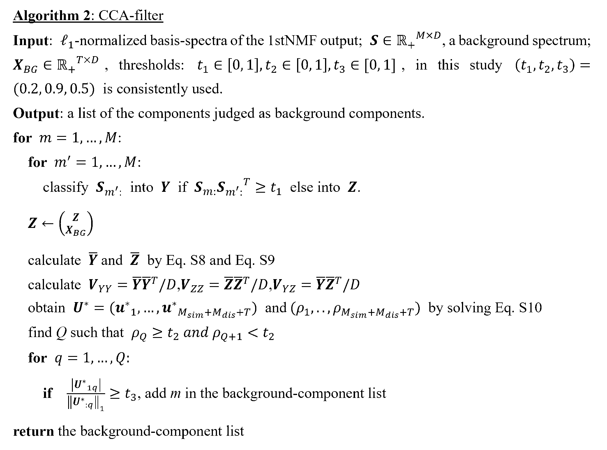
CCA-filterから出力された、バックグラウンドに由来するM′-成分除去済みの












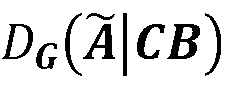


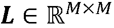




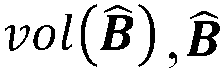
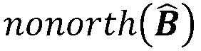











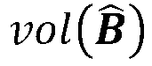
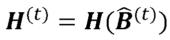


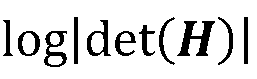


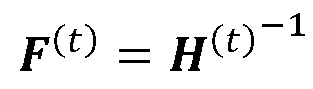










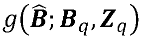




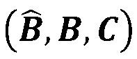





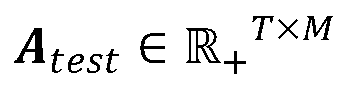
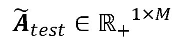
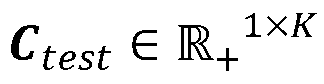
データセットからSとBを推定したのちに、SとBの推定には用いなかったデータ(ここではテストデータと呼ぶ)
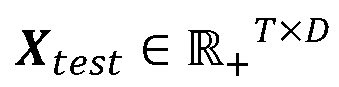
まずS-超平面への射影により、


次に、本発明の実施形態に係る組成推定装置について、図面を参照しながら説明する。図3は、本発明の実施形態に係る組成推定装置のハードウェア構成図である。
記憶デバイス35は、例えば、ROM(Read Only Memory)、RAM(Random Access Memory)、HDD(Hard Disk Drive)、フラッシュメモリ、及び、SSD(Solid State Drive)等である。
また、表示デバイス36は、入力デバイス37と一体として構成されていてもよい。この場合、表示デバイス36がタッチパネルディスプレイであって、GUI(Graphical User Interface)を提供する形態が挙げられる。
質量分析部41は、ロードされた検体セット(検体、学習用検体、及び、バックグラウンド検体、図4中、符号a)について、加熱しながら熱脱着、及び/又は、熱分解されて生ずるガス成分をイオン化し、順次質量分析して、マススペクトルを出力する(図4中、符号c)。
この際、質量分析装置31の設置されている環境に起因した環境要因(図4中、符号b、例えば、減圧ポンプ32から生ずる(ポリ)ジメチルシロキサン)も同時に質量分析装置31にロードされ、マススペクトルに影響を与える。
制御部43は、プロセッサ34を含んで構成される。制御部43は、各部を制御して、組成推定装置30の各機能を実現する。
データ行列作成部47は、質量分析部41によって加熱温度ごとに取得されたマススペクトル(図4中、符号c)を各行に格納した二次元マススペクトルからデータ行列Xを作成し、後述するNMF処理部48に渡す(図4中、符号d)。なお、データ行列Xの詳細については、すでに説明したとおりである。
NMF処理部48は、データ行列作成部47によって作成されたデータ行列X(図4中、符号d)を非負値行列因子分解(NMF)し、規格化された基底スペクトル行列(S)とその強度分布行列(C)との積(X=C×ST)に分解する。その結果は、補正処理部49に渡される(図4中、符号e)。なお、NMF処理の詳細はすでに説明したとおりである。
補正処理部49は、NMF処理部48によって作成された基底スペクトル行列とデータ行列との正準相関分析によって強度分布行列を補正して、補正後強度分布行列を作成する機能である。作成された補正後強度分布行列はベクトル処理部50に渡される(図4中、符号f)。
ベクトル処理部50は、補正処理部49により作成された補正後強度分布行列を全検体のそれぞれに対応する小行列に分割し、これを特徴ベクトルとしてベクトル空間内で全検体を表現する。この結果は、エンドメンバー決定部51に渡される(図4中、符号g)。
エンドメンバー決定部51は、ベクトル処理部50によって作成された特徴ベクトルの全てを内包するK-1次元単体を設定し、K-1次元単体におけるK個のエンドメンバーを決定する。この結果は、含有量比計算部52に渡される(図4中、符号h)。
しかし、すでに説明したとおり、エンドメンバーの決定(エンドメンバー決定部51の処理)には判別ラベルは必須ではない。
含有量比計算部52は、エンドメンバー決定部51によって決定されたK個のエンドメンバーと、ベクトル処理部50により作成された推定対象検体の特徴ベクトルとのユークリッド距離をそれぞれ計算し、K個のエンドメンバーと検体の特徴ベクトルとのユークリッド距離の比から、推定対象検体中のK個の成分の含有量比を推定する。この含有量比の推定結果(図4中、符号i)は、出力部46から出力される。
なお、この際、学習用検体の組成推定結果もあわせて出力してもよい。
(検体の準備)
ポリメチルメタクリレート(poly(methyl methacrylate)、記号「M」)、ポリスチレン(polystyrene、記号「S」)、ポリエチルメタクリレート(poly(ethyl methacrylate)、記号「E」)の三種類の高分子のジオキサン溶液(約4質量%、高分子の固形分として0.4mg程度)を、サンプルポット上にキャストした後に一晩風乾して検体を得た。表4は、各検体の組成である。なお、質量分析は、SHIMADZU社製LCMS-2020を検出器として、IonSense社製DARTイオン源として、バイオクロマト社製イオンロケットをサンプルの加熱部として用いて行った。
(ii)NMF最適化中のマージング条件
(iii)CCA-filterによるNMFアーティファクト、及び、バックグラウンド、コンタミネーション除去
(iv)環境変数を補正項にいれることで、キャリブレーション不要の定量分析
NMF:
orthogonal constrain weight w=0.2, initial component number K=50, small positive number a=1+0.1-15, iteration number L=2000, threshold=0.9
CCA-Filter:
t1=0.8,t2=0.2,
図8の結果から、NMFが直交制約を有する方が、より優れた推定結果が得られることがわかった。
図9の結果から、MNF最適化の条件がmerging Sを有する方が、より優れた推定結果が得られることがわかった。
なお、成分数はARDによって36までしか減らせないが、Merging Sの条件を維持したときは成分数9でより精度よく組成が推定できることから、Merging Sの重要性がわかった。
図10においては、検体「SE」は、Mの含有量は0%にも関わらず1%程度入っているという計算結果となった。0%を1%と推定してしまうと、数%の推定精度もないということになり実用的ではない。
この結果から、CCA-filterを解除すると、DOX、BG(図5の説明を参照)のいずれのノイズも除去できていないことがわかった。
(エンドメンバーを含まない検体による推定)
学習用検体を含む検体(群)が、エンドメンバーを含まない場合にも精度よく推定できることを確かめるために、表5に記載したサンプルを調製して実施例1と同様の試験を行った。
なお、表中、記号「M」「S」「E」が意味するものは、表4(実施例1)と同様である。また、各サンプルは、単独の成分(ポリマー)の重量分率が80%を超えないように調整されている。

図中Cでは、本方法によって、推定された組成を丸印で、使用したサンプルの組成(正しい組成)を星印で示している。いずれもよい一致を示している。
ここでは、使用した検体にエンドメンバー、すなわち、E、S、Mのピュアポリマーが含まれていないことが、Cの各頂点にプロットがないことからもわかる。
なお、テストデータがある場合には、XtestをSとBに連続射影してCtestを得る。
(エンドメンバーを1つ含む検体による推定)
次に、(学習用)検体のうち1つがエンドメンバーを含む場合に、他の検体における成分含有量が任意となる(K-1次元単体の内接円の外側の領域でなくてもよい)ことを検証した。
上記原因のひとつは、すでに説明した2回目のNMF処理(Eq.11)において基底の非直交性項

Claims (21)
- Kを1以上の整数としたとき、K種類の成分から選択される少なくとも1種の前記成分を含む推定対象検体における、前記成分の含有量比を推定する方法であって、
前記K種類の成分から選択される少なくとも1種の成分を含み、互いに組成の異なるK個以上の学習用検体、及び、前記成分を含まないバックグラウンド検体を準備することと、
前記推定対象検体、前記学習用検体、及び、バックグラウンド検体を含む検体セットに含まれるそれぞれの検体を加熱しながら、熱脱着、及び/又は、熱分解によって生ずるガス成分を順次イオン化し、マススペクトルを連続的に観測することと、
加熱温度ごとに得られた前記マススペクトルを各行に格納し、前記検体ごとの二次元マススペクトルを得て、前記二次元マススペクトルの少なくとも2つ以上をまとめてデータ行列に変換することと、
前記データ行列を非負値行列因子分解し、規格化された基底スペクトル行列とその強度分布行列の積に分解するNMF処理を行うことと、
前記基底スペクトル行列と前記データ行列との正準相関分析によって強度分布行列に含まれるノイズ成分を抽出し、前記ノイズ成分の影響を減ずるよう前記強度分布行列を補正して、補正後強度分布行列を得ることと、
前記補正後強度分布行列を前記検体のそれぞれに対応する小行列に分割し、前記小行列を特徴ベクトルとして、ベクトル空間内で前記検体のそれぞれを表現することと、
前記特徴ベクトルの全てを内包するK-1次元単体を設定し、前記K-1次元単体におけるK個のエンドメンバーを決定することと、
前記K個のエンドメンバーと、前記推定対象検体の特徴ベクトルとの、ユークリッド距離をそれぞれ計算し、前記ユークリッド距離の比により、前記推定対象検体中の前記成分の含有量比を推定することと、を含み、
前記Kが3以上の場合、前記K-1次元単体に内接する超球体の外側の領域のそれぞれに、前記学習用検体の特徴ベクトルの少なくとも1つが位置する、又は、前記学習用検体が前記エンドメンバーの少なくとも1つを含む、方法。 - 前記Kが2以上の整数であり、前記推定対象検体が、前記成分の混合物である、請求項1に記載の方法。
- 前記学習用検体が、前記エンドメンバーを含む、請求項1又は2に記載の方法。
- 前記エンドメンバーの決定が、前記学習用検体に付された判別ラベルに基づき行われる、請求項3に記載の方法。
- 前記エンドメンバーの決定が、前記学習用検体の前記特徴ベクトルの頂点成分分析によって行われる、請求項3に記載の方法。
- 前記エンドメンバーの決定が、前記K-1次元単体が最小体積となるように頂点を定めるアルゴリズムによって実施される、請求項1に記載の方法。
- 前記エンドメンバーの決定が、前記補正後強度分布行列を非負値行列因子分解し、前記検体中のK種類の前記成分の重量分率を表す行列と、K種類の個別の前記成分ごとのフラグメント存在強度を表す行列との積に分解する第2のNMF処理により行われる、請求項6に記載の方法。
- 前記学習用検体が、前記エンドメンバーを含まない、請求項6又は7に記載の方法。
- 前記補正後強度分布行列を得ることは、更に、前記強度分布行列の強度補正を行うことを含む、請求項1~8のいずれか1項に記載の方法。
- 前記検体セットが、更に、キャリブレーション検体を含み、
前記キャリブレーション検体は、前記K種類の成分を全て含み、かつ、その組成が既知であり、
前記強度補正は、前記強度分布行列を規格化することを含む、請求項9に記載の方法。 - 前記強度補正は、前記強度分布行列の少なくとも一部を、前記検体セットのうち対応する前記検体の質量と環境変数の積で割り付けることを含み、
前記環境変数は、前記観測の際における前記成分のイオン化効率への影響を表す変数である、請求項9に記載の方法。 - 前記環境変数が、前記観測の際に、雰囲気中に所定量含まれる分子量50~1500の化合物、又は、前記検体セットのそれぞれに所定量含まれる分子量50~500の有機低分子化合物のマススペクトルのピークの合計値である、請求項11に記載の方法。
- Kを1以上の整数としたとき、K種類の成分から選択される少なくとも1種の前記成分を含む推定対象検体における、前記成分の含有量比を推定する組成推定装置であって、
前記K種類の成分から選択される少なくとも1種の成分を含み、互いに組成の異なるK個以上の学習用検体、前記成分を含まないバックグラウンド検体、及び、前記推定対象検体を含む検体セットに含まれるそれぞれの検体を加熱しながら、熱脱着、及び/又は、熱分解によって生ずるガス成分を順次イオン化し、マススペクトルを連続的に観測する質量分析装置と、
前記観測されたマススペクトルを処理する情報処理装置と、を備え、
前記情報処理装置は、
加熱温度ごとに得られた前記マススペクトルを各行に格納し、前記検体ごとの二次元マススペクトルを得て、前記二次元マススペクトルの少なくとも2つ以上をまとめてデータ行列に変換する、データ行列作成部と、
前記データ行列を非負値行列因子分解し、規格化された基底スペクトル行列とその強度分布行列の積に分解するNMF処理を行う、NMF処理部と、
前記基底スペクトル行列と前記データ行列との正準相関分析によって強度分布行列に含まれるノイズ成分を抽出し、前記ノイズ成分の影響を減ずるよう前記強度分布行列を補正して、補正後強度分布行列を作成する、補正処理部と、
前記補正後強度分布行列を前記検体セットのそれぞれに対応する小行列に分割し、前記小行列を特徴ベクトルとして、ベクトル空間内で前記検体のそれぞれを表現する、ベクトル処理部と、
前記特徴ベクトルの全てを内包するK-1次元単体を設定し、前記K-1次元単体におけるK個のエンドメンバーを決定する、エンドメンバー決定部と、
前記K個のエンドメンバーと、前記推定対象検体の特徴ベクトルとの、ユークリッド距離をそれぞれ計算し、前記ユークリッド距離の比により、前記推定対象検体中の前記成分の含有量比を推定する、含有量比計算部と、を含み、
前記Kが3以上の場合、前記K-1次元単体に内接する超球体の外側の領域のそれぞれに、前記学習用検体の特徴ベクトルの少なくとも1つが位置する、又は、前記学習用検体が前記エンドメンバーの少なくとも1つを含む、組成推定装置。 - 前記エンドメンバー決定部は、前記学習用検体に付された判別ラベルに基づいて前記エンドメンバーを決定する、請求項13に記載の組成推定装置。
- 前記エンドメンバー決定部は、前記K-1次元単体が最小体積となるように頂点を定めるアルゴリズムによって前記エンドメンバーを決定する、請求項13に記載の組成推定装置。
- 前記エンドメンバー決定部は、前記補正後強度分布行列を非負値行列因子分解し、前記検体中のK種類の前記成分の重量分率を表す行列と、K種類の個別の前記成分ごとのフラグメント存在強度を表す行列との積に分解する第2のNMF処理により前記エンドメンバーを決定する、請求項15に記載の組成推定装置。
- 前記補正処理部は更に、前記強度分布行列の強度補正を行う、請求項15に記載の組成推定装置。
- 前記検体セットが、更に、キャリブレーション検体を含み、
前記キャリブレーション検体が、前記K種類の成分を全て含み、かつ、その組成が既知であり、
前記強度補正が、前記強度分布行列を規格化することを含む、請求項17に記載の組成推定装置。 - 前記強度補正は、前記強度分布行列の少なくとも一部を、前記検体セットのうち対応する前記検体の質量と環境変数の積で割り付けることを含み、
前記環境変数は、前記観測の際における前記成分のイオン化効率への影響を表す変数である、請求項17に記載の組成推定装置。 - 前記質量分析装置は減圧ポンプを更に備え、
前記環境変数が、前記減圧ポンプの稼働によって生ずる物質のマススペクトルのピークの合計値である、請求項19に記載の組成推定装置。 - Kを1以上の整数としたとき、K種類の成分から選択される少なくとも1種の前記成分を含む推定対象検体における、前記成分の含有量比を推定する組成推定装置において用いられるプログラムであって、
前記K種類の成分から選択される少なくとも1種の成分を含み、互いに組成の異なるK個以上の学習用検体、前記成分を含まないバックグラウンド検体、及び、前記推定対象検体を含む検体セットに含まれるそれぞれの検体を加熱しながら、熱脱着、及び/又は、熱分解によって生ずるガス成分を順次イオン化し、マススペクトルを連続的に観測する質量分析装置と、
前記観測されたマススペクトルを処理する情報処理装置と、を備え、
前記質量分析装置によって、加熱温度ごとに取得された前記マススペクトルを各行に格納し、前記検体ごとの二次元マススペクトルを得て、前記二次元マススペクトルの少なくとも2つ以上をまとめてデータ行列に変換する、データ行列作成機能と、
前記データ行列を非負値行列因子分解し、規格化された基底スペクトル行列とその強度分布行列の積に分解するNMF処理を行う、NMF処理機能と、
前記基底スペクトル行列と前記データ行列との正準相関分析によって強度分布行列に含まれるノイズ成分を抽出し、前記ノイズ成分の影響を減ずるよう前記強度分布行列を補正して、補正後強度分布行列を作成する、補正処理機能と、
前記補正後強度分布行列を前記検体のそれぞれに対応する小行列に分割し、前記小行列を特徴ベクトルとして、ベクトル空間内で前記検体のそれぞれを表現する、ベクトル処理機能と、
前記特徴ベクトルの全てを内包するK-1次元単体を設定し、前記K-1次元単体におけるK個のエンドメンバーを決定する、エンドメンバー決定機能と、
前記K個のエンドメンバーと、前記推定対象検体の特徴ベクトルとの、ユークリッド距離をそれぞれ計算し、前記ユークリッド距離の比により、前記推定対象検体中の前記成分の含有量比を推定する、含有量比計算機能と、を含み、
前記Kが3以上の場合、前記K-1次元単体に内接する超球体の外側の領域のそれぞれに、前記学習用検体の特徴ベクトルの少なくとも1つが位置する、又は、前記学習用検体が前記エンドメンバーの少なくとも1つを含む、プログラム。
Priority Applications (3)
| Application Number | Priority Date | Filing Date | Title |
|---|---|---|---|
| JP2023529793A JP7628731B2 (ja) | 2021-06-24 | 2022-06-06 | 検体に含まれる成分の含有量比の推定方法、組成推定装置、及び、プログラム |
| US18/569,560 US20240297031A1 (en) | 2021-06-24 | 2022-06-06 | Method of inferring content ratio of component in sample, composition inference device, and program |
| EP22828206.7A EP4361624B1 (en) | 2021-06-24 | 2022-06-06 | Method for estimating content ratio of components contained in sample, composition estimating device, and program |
Applications Claiming Priority (2)
| Application Number | Priority Date | Filing Date | Title |
|---|---|---|---|
| JP2021104510 | 2021-06-24 | ||
| JP2021-104510 | 2021-06-24 |
Publications (1)
| Publication Number | Publication Date |
|---|---|
| WO2022270289A1 true WO2022270289A1 (ja) | 2022-12-29 |
Family
ID=84544540
Family Applications (1)
| Application Number | Title | Priority Date | Filing Date |
|---|---|---|---|
| PCT/JP2022/022813 Ceased WO2022270289A1 (ja) | 2021-06-24 | 2022-06-06 | 検体に含まれる成分の含有量比の推定方法、組成推定装置、及び、プログラム |
Country Status (4)
| Country | Link |
|---|---|
| US (1) | US20240297031A1 (ja) |
| EP (1) | EP4361624B1 (ja) |
| JP (1) | JP7628731B2 (ja) |
| WO (1) | WO2022270289A1 (ja) |
Cited By (1)
| Publication number | Priority date | Publication date | Assignee | Title |
|---|---|---|---|---|
| WO2025033010A1 (ja) | 2023-08-09 | 2025-02-13 | 国立研究開発法人物質・材料研究機構 | 組成推定方法、組成推定装置、プログラム、検体容器、及び、熱重量・質量分析方法 |
Citations (5)
| Publication number | Priority date | Publication date | Assignee | Title |
|---|---|---|---|---|
| JP2012516445A (ja) * | 2009-01-27 | 2012-07-19 | ホロジック,インコーポレイテッド | 体液における新生児敗血症の検出のためのバイオマーカー |
| JP2013528287A (ja) * | 2010-06-10 | 2013-07-08 | インターナショナル・ビジネス・マシーンズ・コーポレーション | 質量スペクトルを分析するための方法、コンピュータ・プログラム、およびシステム |
| WO2016120958A1 (ja) * | 2015-01-26 | 2016-08-04 | 株式会社島津製作所 | 3次元スペクトルデータ処理装置及び処理方法 |
| WO2018158801A1 (ja) * | 2017-02-28 | 2018-09-07 | 株式会社島津製作所 | スペクトルデータの特徴抽出装置および方法 |
| JP2021081365A (ja) * | 2019-11-21 | 2021-05-27 | 株式会社島津製作所 | 糖ペプチド解析装置 |
Family Cites Families (2)
| Publication number | Priority date | Publication date | Assignee | Title |
|---|---|---|---|---|
| EP1997049B1 (en) * | 2006-03-21 | 2019-03-13 | Metabolon Inc. | A system, method, and computer program product for analyzing spectrometry data to indentify and quantify individual components in a sample |
| WO2007112597A1 (en) * | 2006-04-05 | 2007-10-11 | National Research Council Of Canada | Blind extraction of pure component mass spectra from overlapping mass spectrometric peaks |
-
2022
- 2022-06-06 JP JP2023529793A patent/JP7628731B2/ja active Active
- 2022-06-06 WO PCT/JP2022/022813 patent/WO2022270289A1/ja not_active Ceased
- 2022-06-06 US US18/569,560 patent/US20240297031A1/en active Pending
- 2022-06-06 EP EP22828206.7A patent/EP4361624B1/en active Active
Patent Citations (5)
| Publication number | Priority date | Publication date | Assignee | Title |
|---|---|---|---|---|
| JP2012516445A (ja) * | 2009-01-27 | 2012-07-19 | ホロジック,インコーポレイテッド | 体液における新生児敗血症の検出のためのバイオマーカー |
| JP2013528287A (ja) * | 2010-06-10 | 2013-07-08 | インターナショナル・ビジネス・マシーンズ・コーポレーション | 質量スペクトルを分析するための方法、コンピュータ・プログラム、およびシステム |
| WO2016120958A1 (ja) * | 2015-01-26 | 2016-08-04 | 株式会社島津製作所 | 3次元スペクトルデータ処理装置及び処理方法 |
| WO2018158801A1 (ja) * | 2017-02-28 | 2018-09-07 | 株式会社島津製作所 | スペクトルデータの特徴抽出装置および方法 |
| JP2021081365A (ja) * | 2019-11-21 | 2021-05-27 | 株式会社島津製作所 | 糖ペプチド解析装置 |
Non-Patent Citations (7)
| Title |
|---|
| "Robust Volume Minimization-based Matrix Factorization for remote Sensing and Document Clustering", IEEE TRANSACTIONS ON SIGNAL PROCESSING, vol. 64, no. 23, 1 December 2016 (2016-12-01) |
| ANALYTICAL CHEMISTRY, vol. 92, 2020, pages 1925 - 1933 |
| J. M. B. DIASJ. M. P. NASCIMENTO: "Vertex component analysis: A geometric-based approach to unmix hyperspectral data", SIGNAL IMAGE PROCESS. REMOTE SENS., vol. 43, 2006, pages 415 - 439 |
| S. BOYDN. PARIKHE. CHUB. PELEATOJ. ECKSTEIN: "Distributed optimization and statistical learning via the alternating direction method of multipliers", FOUND. TRENDS MACH. LEARN., vol. 3, 2010, pages 1 - 122, XP055127725, DOI: 10.1561/2200000016 |
| See also references of EP4361624A4 |
| SHIGA, M. ET AL.: "Sparse modeling of EELS and EDX spectral imaging data by nonnegative matrix factorization", ULTRAMICROSCOPY, vol. 170, 2016, pages 43 - 59 |
| X. FUK. HUANGB. YANGW. K. MAN. D. SIDIROPOULOS: "Robust Volume Minimization-Based Matrix Factorization for Remote Sensing and Document Clustering", IEEE TRANS. SIGNAL PROCESS., vol. 64, 2016, pages 6254 - 6268, XP011625333, DOI: 10.1109/TSP.2016.2602800 |
Cited By (1)
| Publication number | Priority date | Publication date | Assignee | Title |
|---|---|---|---|---|
| WO2025033010A1 (ja) | 2023-08-09 | 2025-02-13 | 国立研究開発法人物質・材料研究機構 | 組成推定方法、組成推定装置、プログラム、検体容器、及び、熱重量・質量分析方法 |
Also Published As
| Publication number | Publication date |
|---|---|
| EP4361624A1 (en) | 2024-05-01 |
| JPWO2022270289A1 (ja) | 2022-12-29 |
| EP4361624A4 (en) | 2025-07-02 |
| EP4361624B1 (en) | 2026-05-06 |
| US20240297031A1 (en) | 2024-09-05 |
| JP7628731B2 (ja) | 2025-02-12 |
Similar Documents
| Publication | Publication Date | Title |
|---|---|---|
| Burger et al. | Data handling in hyperspectral image analysis | |
| JP6089345B2 (ja) | 時および/または空間系列ファイルの多成分回帰/多成分分析 | |
| Gorrochategui et al. | Chemometric strategy for untargeted lipidomics: biomarker detection and identification in stressed human placental cells | |
| Trindade et al. | Non-negative matrix factorisation of large mass spectrometry datasets | |
| CN103959426B (zh) | 用于通过质谱术识别微生物的方法 | |
| Moorthy et al. | Pattern similarity measures applied to mass spectra | |
| CN109738413B (zh) | 基于稀疏非负最小二乘的混合物拉曼光谱定性分析方法 | |
| JP6748085B2 (ja) | 干渉検出および着目ピークのデコンボルーション | |
| Lewis et al. | Comparing multiple statistical methods for inverse prediction in nuclear forensics applications | |
| Koo et al. | Analysis of metabolomic profiling data acquired on GC–MS | |
| Borsoi et al. | Fast unmixing and change detection in multitemporal hyperspectral data | |
| Franceschi et al. | Self‐organizing maps: A versatile tool for the automatic analysis of untargeted imaging datasets | |
| US20240393310A1 (en) | Biomarker reflectance signatures for disease detection and classification | |
| Mani-Varnosfaderani et al. | Estimating complicated baselines in analytical signals using the iterative training of Bayesian regularized artificial neural networks | |
| Gibb et al. | Mass spectrometry analysis using MALDIquant | |
| Rapin et al. | Application of non-negative matrix factorization to LC/MS data | |
| Lalor et al. | Sim-to-real supervised domain adaptation for radioisotope identification | |
| Deng et al. | An infinite Gaussian mixture model with its application in hyperspectral unmixing | |
| JP7757246B2 (ja) | 試料分析装置及び方法 | |
| Teurtrie et al. | From STEM-EDXS data to phase separation and quantification using physics-guided NMF | |
| EP4361624B1 (en) | Method for estimating content ratio of components contained in sample, composition estimating device, and program | |
| Zhang et al. | Chromatographic fingerprinting and chemometric techniques for quality control of herb medicines | |
| JP2008500537A (ja) | 分光計によって生成されたデータからスペクトルを抽出するためのシステム及び方法 | |
| Negoita et al. | Artificial intelligence application designed to screen for new psychoactive drugs based on their ATR-FTIR spectra | |
| Caiafa | On the conditions for valid objective functions in blind separation of independent and dependent sources |
Legal Events
| Date | Code | Title | Description |
|---|---|---|---|
| 121 | Ep: the epo has been informed by wipo that ep was designated in this application |
Ref document number: 22828206 Country of ref document: EP Kind code of ref document: A1 |
|
| WWE | Wipo information: entry into national phase |
Ref document number: 2023529793 Country of ref document: JP |
|
| WWE | Wipo information: entry into national phase |
Ref document number: 18569560 Country of ref document: US |
|
| WWE | Wipo information: entry into national phase |
Ref document number: 2022828206 Country of ref document: EP |
|
| NENP | Non-entry into the national phase |
Ref country code: DE |
|
| ENP | Entry into the national phase |
Ref document number: 2022828206 Country of ref document: EP Effective date: 20240124 |
|
| WWG | Wipo information: grant in national office |
Ref document number: 2022828206 Country of ref document: EP |