WO2019044729A1 - 状態監視方法および状態監視装置 - Google Patents
状態監視方法および状態監視装置 Download PDFInfo
- Publication number
- WO2019044729A1 WO2019044729A1 PCT/JP2018/031476 JP2018031476W WO2019044729A1 WO 2019044729 A1 WO2019044729 A1 WO 2019044729A1 JP 2018031476 W JP2018031476 W JP 2018031476W WO 2019044729 A1 WO2019044729 A1 WO 2019044729A1
- Authority
- WO
- WIPO (PCT)
- Prior art keywords
- waveform
- feature
- feature amount
- waveforms
- value
- Prior art date
- Legal status (The legal status is an assumption and is not a legal conclusion. Google has not performed a legal analysis and makes no representation as to the accuracy of the status listed.)
- Ceased
Links
Images





Classifications
-
- G—PHYSICS
- G01—MEASURING; TESTING
- G01M—TESTING STATIC OR DYNAMIC BALANCE OF MACHINES OR STRUCTURES; TESTING OF STRUCTURES OR APPARATUS, NOT OTHERWISE PROVIDED FOR
- G01M99/00—Subject matter not provided for in other groups of this subclass
-
- G—PHYSICS
- G05—CONTROLLING; REGULATING
- G05B—CONTROL OR REGULATING SYSTEMS IN GENERAL; FUNCTIONAL ELEMENTS OF SUCH SYSTEMS; MONITORING OR TESTING ARRANGEMENTS FOR SUCH SYSTEMS OR ELEMENTS
- G05B23/00—Testing or monitoring of control systems or parts thereof
- G05B23/02—Electric testing or monitoring
Definitions
- the present invention relates to a method and a device for monitoring the state of a device under test such as a rotary machine.
- the state of the test object is monitored based on measurement data of physical quantities measured by various sensors. Specifically, a feature amount indicating the feature of the waveform indicated by the measurement data is calculated, and the presence or absence of an abnormality of the test object is determined using the calculated feature amount.
- Patent Document 1 determines the presence or absence of abnormality using a set of a frequency at which a peak obtained from a time change of a spectrum of waveform data occurs and a time interval at which the peak occurs. Methods for diagnosing abnormalities are disclosed.
- Patent Document 2 determines the presence or absence of abnormality of equipment using the minimum distance between each neuron of the clustering map and the neuron corresponding to the frequency component extracted from the signal during operation of the equipment. A method of monitoring equipment is disclosed.
- Patent Document 1 Japanese Patent Application Laid-Open No. 2006-300895
- the present invention has been made to solve the above-mentioned problems, and an object thereof is to provide a state monitoring method and a state monitoring apparatus with high accuracy in determining the presence or absence of an abnormality of an object to be tested.
- the present invention is a state monitoring method for monitoring the state of an object under test using measurement data acquired from a sensor installed on the object under test.
- the condition monitoring method includes first to fourth steps.
- a plurality of first waveforms respectively corresponding to the plurality of band pass filters are generated by performing filter processing on each of the plurality of band pass filters having center frequencies different from each other on the measurement data.
- a first feature amount is calculated for each of the plurality of first waveforms.
- the center frequency is taken on the horizontal axis
- the first feature value is taken on the vertical axis
- each of the plurality of band pass filters is generated using the center frequency of the band pass filter and the band pass filter.
- a second feature amount indicating a feature of a second waveform obtained by plotting the calculated first feature amount with respect to the calculated time waveform is calculated.
- the test target object based on the second feature value calculated by performing the first to third steps on the test data obtained from the sensor at the time of diagnosis of the test object among the measurement data. Determine if the object is abnormal.
- the plurality of first waveforms are time waveforms.
- the first feature quantity includes a first waveform corresponding to the first feature quantity among the plurality of first waveforms, a third waveform obtained by Fourier transforming the corresponding first waveform, and a Fourier transform of the third waveform. And the characteristic of any one waveform with the fourth waveform obtained.
- the plurality of first waveforms are time waveforms.
- the second step Fourier-transforms the first waveform corresponding to the first feature amount among the plurality of first waveforms, the third waveform obtained by Fourier-transforming the corresponding first waveform, and the third waveform.
- a step of calculating a third feature value indicating the feature of the waveform and a third feature value calculated for each of the at least two waveforms 1 includes the step of calculating the feature amount.
- the second feature value obtained by performing the first to third steps on normal data obtained from the sensor when the test object is normal among the measurement data is used as learning data.
- the method further comprises a fifth step of determining an algorithm for determining whether the object under test is abnormal by performing machine learning. In a fourth step, it is determined whether or not the object under test is abnormal according to an algorithm.
- the second feature value is any one of an effective value, a maximum value, a crest factor, a kurtosis, a skewness, a variation coefficient, and a contribution rate of the second waveform.
- the present invention in another aspect, is a condition monitoring apparatus that diagnoses an object under test using any of the above-described methods.
- the state monitoring method of the present invention can increase the determination accuracy of the presence or absence of abnormality of the device under test.
- FIG. 18 is a diagram showing a t-test result of the second feature value calculated by the data calculation method of the embodiment in verification experiment 2. It is a figure which shows t examination result of the feature-value for comparison calculated by the data calculation method of a comparative example. It is a figure showing an example of the 1st feature quantity of a modification.
- FIG. 18 is a diagram showing a t-test result of the second feature amount in verification experiment 3.
- FIG. 18 is a diagram showing the result of t-test of the second feature amount in verification experiment 4.
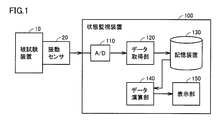
- FIG. 1 is a block diagram showing the configuration of the state monitoring device according to the present embodiment.
- the state monitoring apparatus 100 receives a vibration acceleration signal from a vibration sensor 20 installed in the device under test 10, monitors the state of the device under test 10, and determines the presence or absence of abnormality.
- the device under test 10 is a facility including a rotary machine installed, for example, in a factory or a power plant, and the vibration sensor 20 can detect abnormal vibration generated during rotation.
- the vibration sensor 20 that outputs the vibration acceleration signal is illustrated, but any output signal that can confirm the operating condition of the facility may be a detection signal other than the vibration sensor.
- a sensor that outputs a signal indicating a physical quantity such as speed, displacement, sound, AE (Acoustic Emission), temperature, load torque, or motor power may be used instead of the vibration sensor 20.
- the state monitoring device 100 includes an A / D converter 110, a data acquisition unit 120, a storage device 130, a data calculation unit 140, and a display unit 150.
- the A / D converter 110 receives the vibration acceleration signal of the vibration sensor 20, converts it into a digital signal, and outputs it.
- the data acquisition unit 120 receives the vibration acceleration signal in digital form from the A / D converter 110, performs noise removal processing, and generates measurement data indicating a change in the vibration acceleration for a predetermined time (for example, 20 seconds).
- the data acquisition unit 120 records the generated measurement data in the storage device 130.
- the data operation unit 140 reads measurement data (normal data) measured at normal times from the storage device 130, determines an algorithm for determining the presence or absence of abnormality, or measures at the time of test using the algorithm. From the measurement data (test data), it is determined whether or not there is an abnormality in the device under test 10. When the data calculation unit 140 determines the presence or absence of an abnormality, the data calculation unit 140 causes the display unit 150 to display the determination result.
- FIG. 2 is a block diagram showing details of the data calculation unit.
- the data calculation unit 140 includes a filter processing unit 141, a feature quantity calculation unit 142, a learning unit 143, a threshold storage unit 144, and a determination unit 146.
- the filter processing unit 141 performs a filtering process on the measurement data stored in the storage device 130 using each of a plurality of band pass filters (BPF (Band-pass Filter)) having center frequencies different from each other. And generating a plurality of time waveforms (first waveforms) respectively corresponding to the plurality of band pass filters.
- BPF Band-pass Filter
- the feature amount calculation unit 142 calculates a first feature amount for each of the plurality of time waveforms generated by the filter processing unit 141. Furthermore, the feature quantity calculator 142 arranges the first feature quantities in the order of low center frequency of the band pass filter for each measurement data (hereinafter referred to as “center frequency waveform”) (second waveform). Generate The feature amount calculation unit 142 calculates, for each measurement data, a second feature amount indicating the feature of the center frequency waveform corresponding to the measurement data.
- the learning unit 143 performs machine learning using, as learning data, a plurality of second feature values respectively calculated for a plurality of measurement data (normal data) acquired when the device under test 10 is normal (initial state etc.) Thus, an algorithm for determining whether the device under test 10 is abnormal is determined.
- the learning unit 143 causes the threshold storage unit 144 to store the determined algorithm.
- the determination unit 146 uses the second feature value calculated for the measurement data (test data) obtained at the time of diagnosis of the device under test 10 according to the algorithm stored in the threshold value storage unit 144. Determine if there is an abnormality in
- FIG. 3 is a flowchart for explaining the process performed by the data acquisition unit of FIG.
- the data acquisition unit 120 receives a digital vibration acceleration signal, and generates data indicating a change in vibration acceleration for a predetermined time (for example, 20 seconds).
- the data acquisition unit 120 performs appropriate filtering among the generated data, such as a low pass filter, a band pass filter, or a high pass filter, to generate measurement data from which basic noise is removed.
- the data acquisition unit 120 stores the generated measurement data in the storage device 130.
- the data acquisition unit 120 stores measurement data acquired when it is known that the device under test 10 operates normally at the initial state of the device under test 10 or at the time of repair completion, etc., in the storage device 130 as normal data.
- the data acquisition unit 120 stores measurement data acquired when it is desired to make a diagnosis while using the device under test 10 as test data in the storage device 130.
- the data acquisition unit 120 automatically acquires test data at a time (for example, every two hours) designated by a timer or the like.
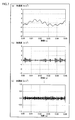
- FIG. 4 is a view showing an example of measurement data acquired by the data acquisition unit 120.
- FIG. 5 is a diagram showing another example of measurement data acquired by the data acquisition unit 120.
- FIG. 4 and 5 show temporal changes in vibration acceleration when the device under test 10 is a bearing.
- Figure 4 shows the measured data when artificially providing a cylindrical damage with a diameter of 1.35 mm in the bearing raceway surface, and Figure 5 artificially creates a larger damage in the bearing raceway surface.
- FIG. 6 is a flowchart for explaining the processing performed by the filter processing unit 141 and the feature quantity calculation unit 142 in FIG.
- the filter processing unit 141 performs filter processing on the measurement data using each of a plurality of band pass filters having different center frequencies.
- the bandwidths of the plurality of band pass filters are not particularly limited, and may be constant (for example, 1 kHz) or may be different from each other.
- the center frequencies of the plurality of band pass filters may be at regular intervals (for example, 1 kHz) or at irregular intervals.
- the band of one band pass filter among the plurality of band pass filters may not overlap with the band of any of the remaining band pass filters, or may overlap with the band of any of the remaining band pass filters. May be
- the filter processing unit 141 generates a plurality of time waveforms respectively corresponding to a plurality of band pass filters.
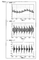
- FIG. 7 shows three time waveforms generated from the measurement data of FIG.
- FIG. 8 shows three time waveforms generated from the measurement data of FIG.
- FIGS. 7 and 8A show time waveforms generated using a band pass filter having a pass band of 0 to 1 kHz.
- FIGS. 7 and 8B show time waveforms generated using a band pass filter having a pass band of 1 to 2 kHz.
- FIGS. 7 and 8C show time waveforms generated using a band pass filter having a pass band of 9 to 10 kHz. As shown in FIGS. 7 and 8, the time waveform differs depending on the frequency band.
- the feature quantity calculation unit 142 calculates a first feature quantity for each of the plurality of time waveforms.
- the first feature quantity is a time domain feature quantity indicating the feature of the corresponding time waveform, and a frequency domain feature quantity indicating the feature of the frequency waveform (third waveform) obtained by Fourier transforming the time waveform.
- a quefence region feature value that indicates the feature of a quefrance waveform (fourth waveform) obtained by Fourier transform of the frequency waveform as a time waveform.
- the first feature value is, for example, the effective value, maximum value, crest factor, kurtosis, skewness, peak-to-peak value, variation coefficient, standard deviation, variance, correlation coefficient, contribution rate, waveform after envelope processing of waveform Is the effective value of Alternatively, the first feature value may be a common logarithm of any value of these parameters.
- the correlation coefficient is a coefficient that indicates the degree of the relationship (for example, a linear relationship) of the distribution law of two random variables (here, time, frequency or quefency and acceleration).
- the contribution rate is the square value of the correlation coefficient.
- the feature quantity calculation unit 142 generates a center frequency waveform with the center frequency of the band pass filter as a variable. That is, the feature quantity calculation unit 142 sets the center frequency of the band pass filter on the horizontal axis and the first feature quantity on the vertical axis, and for each of the plurality of band pass filters, the center frequency of the band pass filter; A center frequency waveform is generated by plotting points indicating the calculated first feature amount with respect to the time waveform corresponding to the band pass filter.
- FIG. 9 is a diagram showing an example of the center frequency waveform.
- FIG. 9 shows a center frequency waveform when the first feature value is the maximum value of the frequency waveform.
- the center frequency waveform described as “damage size 1.35 mm” shows the waveform generated from the measurement data of FIG. 4 and the center frequency waveform described as “no damage” is the device under test 10 And a waveform generated from measurement data when no damage is found in the bearing.
- the shape of the center frequency waveform without damage is different from the shape of the center frequency waveform with damage. This means that the shape of the center frequency waveform is affected by the presence or absence of damage.
- the feature amount calculation unit 142 When the plurality of types of first feature amounts are calculated, the feature amount calculation unit 142 generates a plurality of center frequency waveforms corresponding to each of the plurality of types of first feature amounts.
- the feature quantity calculation unit 142 calculates a second feature quantity indicating the feature of the center frequency waveform.
- the second feature value is, for example, the effective value, maximum value, crest factor, kurtosis, skewness, peak-to-peak value, variation coefficient, standard deviation, variance, correlation coefficient and contribution rate of the center frequency waveform, and envelope processing It is one of the effective values of the later center frequency waveform.
- the correlation coefficient is a coefficient that indicates the degree of the relationship (for example, the linear relationship) of the distribution law of two random variables (here, the center frequency and the first feature value).
- the contribution rate is the square value of the correlation coefficient.
- a sample correlation coefficient can be used as the correlation coefficient.
- the correlation coefficient is calculated using the value of the first feature quantity in the center frequency of the specific range. It may be done.
- the feature amount calculation unit 142 may calculate one type of second feature amount or one or more types of second feature amounts for one center frequency waveform. For example, the feature amount calculation unit 142 may calculate seven types of second feature amounts of the effective value, the maximum value, the crest factor, the kurtosis, the skewness, the variation coefficient, and the contribution rate for the center frequency waveform. .
- FIG. 10 is a flowchart for explaining the process performed by the learning unit 143 in FIG.
- the learning unit 143 acquires the second feature values calculated from the plurality of pieces of normal data measured in the first normal period in which the device under test 10 is normal.
- step S22 the learning unit 143 performs machine learning using the second feature value acquired in step S21 as learning data, and determines an arithmetic expression for calculating an abnormality degree for determining the presence or absence of an abnormality. Specifically, the learning unit 143 determines a classification boundary between abnormal and normal from the learning data, using a known machine learning method (One Class Support Vector Machine: OC-SVM). Then, the learning unit 143 sets the distance from the determined classification boundary as the abnormality degree, and determines an arithmetic expression for calculating the abnormality degree.
- a known machine learning method One Class Support Vector Machine: OC-SVM
- the feature quantity calculation unit 142 can calculate m first feature quantities of m types (m is an integer of 1 or more) for one measurement data, and can be calculated as one type of first feature quantity.
- n types (n is an integer of 1 or more) of second feature amounts. Therefore, there are m ⁇ n types of second feature amounts output from the feature amount calculating unit 142 for one measurement data.
- the learning unit 143 generates a feature amount vector as a component of each of m ⁇ n types of second feature amounts calculated for one normal data.
- the learning unit 143 uses OC-SVM to determine classification boundaries from the same number of feature quantity vectors as the number of normal data, and determines an arithmetic expression for calculating an abnormality degree that is a distance from the determined classification boundaries. Do.
- step S23 the learning unit 143 acquires the second feature values calculated from the plurality of pieces of normal data measured in the second normal period in which the device under test 10 is normal.
- the second normal period is a period after the first normal period.
- step S24 the learning unit 143 calculates the degree of abnormality using the second feature value acquired in step S23 for each normal data, according to the arithmetic expression determined in step S22.
- step S25 the learning unit 143 determines an abnormality determination threshold based on the variation in the degree of abnormality calculated for each piece of normal data.
- the learning unit 143 determines a value obtained by adding a constant multiple (for example, three times) of the standard deviation of the abnormality degree to the average value of the abnormality degree as the abnormality determination threshold value.
- the learning unit 143 uses an arithmetic expression of the degree of abnormality determined in step S22 and the abnormality determination threshold determined in step S25 as an algorithm for determining whether the device under test 10 is abnormal or not. It is stored in the threshold storage unit 144.
- step S23 is omitted, and in step S24, the learning unit 143 calculates the degree of abnormality using the second feature value acquired in step S21 for each normal data according to the arithmetic expression determined in step S22. It is also good.
- FIG. 11 is a flowchart for explaining the process performed by the determination unit 146 in FIG.
- the determination unit 146 acquires a second feature value calculated from measurement data (test data) measured at the time of diagnosis of the device under test 10.
- the determination unit 146 calculates the degree of abnormality using the second feature amount acquired in step S ⁇ b> 31 in accordance with the arithmetic expression stored in the threshold storage unit 144.
- the determination unit 146 compares the abnormality degree calculated in step S32 with the abnormality determination threshold value stored in the threshold value storage unit 144, and based on the comparison result, the abnormality of the device under test 10 is determined. Determine the presence or absence.
- Verification experiment 1 of the effect of the present embodiment Verification experiments were conducted to verify that the degree of abnormality calculated by the above state monitoring method is superior to the degree of abnormality calculated by a known method.
- a non-damaged new bearing was used as the device under test, and the bearing was continuously operated until an abnormality occurred and it became unusable.
- Measurement data of vibration acceleration measured by a vibration sensor installed in a bearing was acquired every two hours. Operating conditions and measurement conditions are as follows.
- Bearings Angular contact ball bearings (Model number 7216: Inner diameter 80 mm, Outer diameter 140 mm, Width 26 mm) Radial load: 1.3kN Axial load: 1.3kN Rotational speed: 1500 revolutions / minute Lubrication method: Grease ⁇ Measurement conditions> Measurement data: Vibration acceleration data length: 20 seconds Sampling speed: 50 kHz.
- the data calculation method in the embodiment was as follows.
- ⁇ Processing method by the filter processing unit 141 With 20 kHz bandwidth of each band pass filter, spacing 1 kHz between center frequencies of a plurality of band pass filters, and a frequency range of 0 to 20 kHz, 20 time waveforms are generated from one measurement data .
- First feature amount calculated by the feature amount calculation unit 142 for one measurement data 6 types (effective value and kurtosis of each of a time waveform, a frequency waveform, and a quefrency waveform).
- Second feature quantity that the feature quantity calculation unit 142 calculates for one center frequency waveform 7 types (effective value, maximum value, crest factor, kurtosis, skewness, variation coefficient, contribution rate).
- the contribution rate is the square of the correlation coefficient between the center frequency and the first feature value in the center frequency range of 1.5 to 9.5 kHz.
- the machine learning method of the learning unit 143 OS-SVM.
- 6 ⁇ 7 42 kinds of second feature amounts calculated from each of the first to predetermined initial measurement data (normal data) in the measurement data group are components.
- the data calculation method of the comparative example was as follows.
- -Feature quantity to be used each of a time waveform represented by measurement data, a frequency waveform obtained by Fourier transforming the time waveform, and a quefrance waveform obtained by Fourier transforming the frequency waveform regarded as the time waveform
- OS-SVM OS-SVM.
- a feature amount vector having the above-mentioned 15 types of feature amounts calculated from each of the first to predetermined initial measurement data (normal data) in the measurement data group is used as a component
- an arithmetic expression of the degree of abnormality was determined.
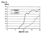
- FIG. 12 is a diagram showing changes in the degree of abnormality between the example and the comparative example.
- the degree of abnormality calculated from the same measurement data group the time when the degree of abnormality of the example starts to increase is compared to the time when the degree of abnormality of the comparative example starts to increase.
- the abnormality degree calculated by the embodiment is a value reflecting a slight abnormality of the bearing. As described above, it was confirmed that the presence or absence of an abnormality in the bearing can be determined with high accuracy by using the abnormality degree calculated in the embodiment.
- the artificial damage is a fine cylindrical hole provided in the outer ring raceway of the bearing by electric discharge machining.
- the vibration acceleration was measured when these bearings were operated at a constant rotational speed under radial load and axial load. The rotational speed was set to three conditions.
- the discharge hole diameter (hereinafter, damage size) is of the following five types (damage size of 0.00 mm indicates a non-damaged bearing). The vibration acceleration was measured 36 times at each damage size. Operating conditions and measurement conditions are as follows.
- Bearings Angular contact ball bearings (Model number 7216: Inner diameter 80 mm, Outer diameter 140 mm, Width 26 mm) Radial load: 1.3kN Axial load: 1.3kN Rotational speed: 1000 revolutions / min, 1500 revolutions / min, 2000 revolutions / min.
- Lubrication method Circulating oil damage size: 0.00 mm (no damage), ⁇ 0.34 mm, ⁇ 0.68 mm, ⁇ 1.02 mm, ⁇ 1.35 mm
- Measurement data Vibration acceleration data length: 20 seconds
- Sampling speed 50 kHz Number of measurements: 36 times.
- the data calculation method in the embodiment was as follows.
- ⁇ Processing method by the filter processing unit 141 With 20 kHz bandwidth of each band pass filter, spacing 1 kHz between center frequencies of a plurality of band pass filters, and a frequency range of 0 to 20 kHz, 20 time waveforms are generated from one measurement data .
- First feature amount calculated by the feature amount calculation unit 142 for one measurement data 6 types (effective value and kurtosis of each of a time waveform, a frequency waveform, and a quefrency waveform).
- Second feature quantity that the feature quantity calculation unit 142 calculates for one center frequency waveform 7 types (effective value, maximum value, crest factor, kurtosis, skewness, variation coefficient, contribution rate).
- the contribution rate is a square of the correlation coefficient between the center frequency and the first feature amount in the center frequency range of 1.5 to 9.5 kHz.
- the data calculation method of the comparative example was as follows.
- -Feature quantity to be used (hereinafter referred to as "comparison feature quantity”): A time waveform represented by measurement data, a frequency waveform obtained by Fourier transforming the time waveform, and a frequency waveform considering the frequency waveform as a time waveform A total of 15 types of effective value, maximum value, crest factor, kurtosis, and skewness of each with the quefrency waveform obtained by conversion.
- Feature amount calculated from measurement data corresponding to a non-damaged bearing (the second feature amount in the example, a comparison feature amount in the comparative example) and feature amount calculated from the measurement data corresponding to the damaged bearing Then, the difference with the second feature value (comparative feature value in the comparative example) was evaluated using a t-test.
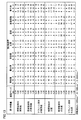
- FIG. 13 is a diagram showing a t-test result of the second feature amount calculated by the data calculation method of the embodiment.
- FIG. 14 is a diagram showing t examination results of the comparison feature value calculated by the data calculation method of the comparative example.
- the test result is the absolute value of the common logarithm value.
- the numerical value is 10 or more
- the feature amount indicating a numerical value of 10 or more has a good sensitivity to the abnormality of the bearing. Therefore, the determination accuracy of the presence or absence of abnormality of a bearing improves by using the feature-value which shows ten or more numerical values.
- the t-test results of the example are generally superior to the t-test results of the comparative example.
- the feature quantity whose t test result is 30 or more under the condition of rotational speed 1000 times / minute and damage size ⁇ 1.35 mm is one type in the data calculation method of the comparative example, whereas the feature quantity is one type. There were seven types.
- the wave height factor, the kurtosis, the skewness and the variation coefficient of the center frequency waveform having the kurtosis of the frequency waveform as the first feature amount, and the effective value of the time waveform as the first feature amount The “contribution rate" of the center frequency waveform that is the feature quantity, the “contribution rate” of the center frequency waveform that uses the effective value of the frequency waveform as the first feature quantity, and the center frequency that has the eff It is the "contribution rate" of the waveform.
- the "contribution rate” of the center frequency waveform which uses the effective value of the quefrance waveform as the first feature value indicates the examination result of 40 or more, and it has excellent sensitivity to the abnormality of the bearing.
- the “effective value”, “maximum value”, and “variation coefficient” of the central frequency waveform having the kurtosis of the frequency waveform as the first feature value, and the center having the effective value of the time waveform as the first feature value The “contribution rate” of the frequency waveform, the “contribution rate” of the center frequency waveform with the effective value of the frequency waveform as the first feature quantity, and the “contribution rate of the center frequency waveform with the effective value of the quefrance waveform as the first feature quantity ".
- These second feature quantities have excellent sensitivity to bearing abnormalities regardless of the rotational speed.
- the “contribution rate” of the center frequency waveform whose first feature value is the effective value of the frequency waveform, is the result of examination of all three rotational speeds, even for bearings with a damage size of ⁇ 0.6 mm or more. The above is shown.
- the second feature quantities calculated by the data calculation method of the embodiment include feature quantities that exhibit excellent sensitivity to bearing abnormalities.
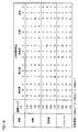
- FIG. 16 is a diagram showing the result of t-test of the second feature amount in verification experiment 3.
- the test result shown in FIG. 16 is the absolute value of the common logarithm value as in FIG.
- the t-test result of verification experiment 3 is also generally superior to the t-test result of the comparative example (see FIG. 14). That is, even if the range of the center frequency of the band pass filter was not limited when obtaining the contribution rate, the contribution rate had excellent sensitivity to the abnormality of the bearing.
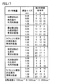
- FIG. 17 is a diagram showing the result of t-test of the second feature amount in verification experiment 4.
- the test result shown in FIG. 17 is an absolute value of a commonly used logarithmic value as in FIG.
- the t-test result of verification experiment 4 is also generally superior to the t-test result of the comparative example (see FIG. 14). That is, even if the common logarithm value of the value of the parameter is used as the first feature amount, the contribution rate has excellent sensitivity to the abnormality of the bearing.
- the feature quantity calculation unit 142 uses the time domain feature quantity that indicates the feature of the time waveform generated using the band pass filter, and the frequency that indicates the feature of the frequency waveform obtained by Fourier transforming the time waveform.
- One of the region feature amount and the quefency region feature amount that indicates the feature of the quefency waveform obtained by subjecting the frequency waveform to Fourier transform is calculated as a first feature amount.
- the feature quantity calculation unit 142 calculates at least two feature quantities of the above-described time domain feature quantity, frequency domain feature quantity, and quefrance domain feature quantity, and the at least two steps.
- a step of calculating a first feature amount from the feature amount may be performed.
- the feature quantity calculation unit 142 calculates the correlation between at least two of the time domain feature quantity (third feature quantity), the frequency domain feature quantity (third feature quantity), and the quefrance area feature quantity (third feature quantity). Values (sum, difference, ratio, average) and the like to be shown are calculated as the first feature amount.
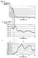
- FIG. 15 is a diagram illustrating an example of the first feature amount of the modification.
- (a) shows the maximum value p of the frequency waveform, which is one of the frequency domain feature quantities
- (b) shows the maximum value q of the quefrance waveform, which is one of the quefrency domain feature quantities.
- (C) shows a first feature quantity.
- the feature amount calculation unit 142 determines, for each of the plurality of band pass filters, the maximum value p of the frequency waveform obtained from the time waveform generated using the band pass filter, and the frequency p The ratio (q / p) to the maximum value q of the quefrance waveform obtained from the waveform is calculated as the first feature value.
- the learning unit 143 performs machine learning using the OC-VSM.
- the learning unit 143 may perform machine learning using random forests, logistic regression, decision trees, and neural networks in addition to SVM.
- the feature quantity calculation unit 142 may calculate only the specific second feature quantity.
- the learning unit 143 determines only the abnormality determination threshold value.
- the determination unit 146 may determine the presence or absence of an abnormality of the device under test 10 based on the comparison result of the second feature amount calculated for the test data and the abnormality determination threshold value.
- the state monitoring method is a method of monitoring the state of the device under test 10 using measurement data acquired from the vibration sensor 20 installed in the device under test (test object) 10.
- a plurality of time waveforms respectively corresponding to the plurality of band pass filters are subjected to filter processing using each of the plurality of band pass filters having center frequencies different from each other on the measurement data. (1st waveform) is generated.
- a first feature amount is calculated for each of the plurality of time waveforms.
- the center frequency of the band pass filter and the band pass A second feature amount indicating a feature of a center frequency waveform (second waveform) obtained by plotting the first feature amount calculated with respect to the time waveform generated using the filter is calculated.
- the fourth step (S32, S33) based on the second feature amount calculated by performing the first to third steps on the test data obtained from the sensor at the time of diagnosis of the device under test 10 among the measurement data. Then, it is determined whether the device under test 10 is abnormal.
- the device under test 10 is abnormal or not based on the second feature amount that has a high sensitivity to the failure of the device under test 10.
- the determination accuracy of the presence or absence of abnormality of the to-be-tested apparatus 10 can be raised.
- an abnormality of the device under test 10 can be detected early.
- the second feature value indicates the feature of the center frequency waveform.
- the center frequency waveform is obtained by plotting the center frequency of each of the plurality of band pass filters and the corresponding first feature amount in a graph in which the center frequency is the horizontal axis and the first feature amount is the vertical axis.
- step S22, S24, S25 of determining an algorithm for determining whether the device under test 10 is abnormal or not is further provided.
- steps S32 and S33 the determination unit 146 determines whether the device under test 10 is abnormal according to the algorithm.
- the first feature value may be, for example, a corresponding time waveform, a frequency waveform (third waveform) obtained by subjecting the time waveform to Fourier transform, and a kerfness waveform obtained by subjecting the frequency waveform to Fourier transform
- the 4th waveform shows the characteristic of one of the waveforms.
- step S12 the time waveform corresponding to the first feature amount among the plurality of time waveforms, the frequency waveform obtained by subjecting the corresponding time waveform to Fourier transform, and the frequency waveform are regarded as the time waveform to perform Fourier transform Calculating, for each of the at least two waveforms, a feature quantity (third feature quantity) indicating the feature of the waveform for each of at least two waveforms with the quefrency waveform obtained by Calculating the first feature amount from the feature amount.
- a feature quantity third feature quantity
- the second feature value is, for example, one of the effective value, maximum value, crest factor, kurtosis, skewness, coefficient of variation, and contribution rate of the second waveform.
- vibration sensor 100 condition monitoring device 110 A / D converter 120 data acquisition unit 130 storage device 140 data operation unit 141 filter processing unit 142 feature amount calculation unit 143 learning unit 144 Threshold storage unit, 146 determination unit, 150 display unit.
Landscapes
- Physics & Mathematics (AREA)
- General Physics & Mathematics (AREA)
- Engineering & Computer Science (AREA)
- Automation & Control Theory (AREA)
- Testing Of Devices, Machine Parts, Or Other Structures Thereof (AREA)
Abstract
状態監視方法は、測定データに対して、互いに異なる中心周波数を有する複数のバンドパスフィルタの各々を用いたフィルタ処理を行なうことにより、複数の第1波形を生成する第1工程と、複数の第1波形の各々に対して第1特徴量を算出する第2工程と、中心周波数を横軸とし、第1特徴量を縦軸とするグラフに、複数のバンドパスフィルタの各々について、当該バンドパスフィルタの中心周波数と、当該バンドパスフィルタを用いて生成された時間波形の第1特徴量とをプロットすることにより得られる第2波形の特徴を示す第2特徴量を算出する第3工程と、テストデータに対して第1~第3工程を行なうことにより算出された第2特徴量に基づいて、被試験対象物が異常か否かを判定する第4工程とを備える。
Description
本発明は、回転機械等の被試験装置の状態監視方法および状態監視装置に関する。
従来、回転機械等の被試験対象物では、各種センサが測定した物理量の測定データに基づいて、被試験対象物の状態を監視している。具体的には、測定データによって示される波形の特徴を示す特徴量が算出され、算出された特徴量を用いて被試験対象物の異常の有無が判定される。
異常の有無の判定精度は、特徴量の異常に対する感度に依存する。そのため、様々な特徴量を用いた状態監視方法が開発されている。たとえば、特開平10-274558号公報(特許文献1)には、波形データのスペクトルの時間変化から求めたピークが生じる周波数と、当該ピークが生じる時間間隔との組を用いて異常の有無を判定する異常診断方法が開示されている。特開2006-300895号公報(特許文献2)には、クラスタリングマップの各ニューロンと設備の運転時の信号から抽出した周波数成分に対応するニューロンとの最小距離を用いて設備の異常の有無を判定する設備監視方法が開示されている。
しかしながら、被試験対象物の異常の有無の判定の精度をさらに向上させることが望まれている。
この発明は、上記の課題を解決するためになされたものであって、その目的は、被試験対象物の異常の有無の判定精度の高い状態監視方法および状態監視装置を提供することである。
この発明は、被試験対象物に設置したセンサから取得した測定データを用いて被試験対象物の状態を監視する状態監視方法である。状態監視方法は、第1~第4工程を備える。第1工程では、測定データに対して、互いに異なる中心周波数を有する複数のバンドパスフィルタの各々を用いたフィルタ処理を行なうことにより、複数のバンドパスフィルタにそれぞれ対応する複数の第1波形を生成する。第2工程では、複数の第1波形の各々に対して第1特徴量を算出する。第3工程では、中心周波数を横軸とし、第1特徴量を縦軸とするグラフに、複数のバンドパスフィルタの各々について、当該バンドパスフィルタの中心周波数と、当該バンドパスフィルタを用いて生成された時間波形に対して算出された第1特徴量とをプロットすることにより得られる第2波形の特徴を示す第2特徴量を算出する。第4工程では、測定データのうち被試験対象物の診断時にセンサから得られたテストデータに対して第1~第3工程を行なうことにより算出された第2特徴量に基づいて、被試験対象物が異常か否かを判定する。
好ましくは、複数の第1波形は時間波形である。第1特徴量は、複数の第1波形の中の当該第1特徴量に対応する第1波形と、対応する第1波形をフーリエ変換して得られる第3波形と、第3波形をフーリエ変換して得られる第4波形とのいずれか1つの波形の特徴を示す。
好ましくは、複数の第1波形は時間波形である。第2工程は、複数の第1波形の中の第1特徴量に対応する第1波形と、対応する第1波形をフーリエ変換して得られる第3波形と、第3波形をフーリエ変換して得られる第4波形との少なくとも2つの波形の各々に対して、当該波形の特徴を示す第3特徴量を算出する工程と、少なくとも2つの波形の各々に対して算出した第3特徴量から第1特徴量を算出する工程とを含む。
好ましくは、状態監視方法は、測定データのうち被試験対象物の正常時にセンサから得られた正常データに対して第1~第3工程を行なうことにより得られた第2特徴量を学習データとして機械学習を行なうことにより、被試験対象物が異常か否かを判定するためのアルゴリズムを決定する第5工程をさらに備える。第4工程では、アルゴリズムに従って前記被試験対象物が異常か否かを判定する。
好ましくは、第2特徴量は、第2波形の実効値、最大値、波高率、尖度、歪度、変動係数および寄与率のいずれかである。
この発明は、他の局面においては、上記のいずれかの方法を用いて、被試験対象物を診断する、状態監視装置である。
本発明の状態監視方法は、被試験装置の異常の有無の判定精度を高めることができる。
以下、本発明の実施の形態について図面を参照しつつ説明する。なお、以下の図面において同一または相当する部分には同一の参照番号を付し、その説明は繰返さない。
[状態監視装置の基本構成]
図1は、本実施の形態に係る状態監視装置の構成を示すブロック図である。図1を参照して、状態監視装置100は、被試験装置10に設置された振動センサ20から振動加速度信号を受けて、被試験装置10の状態を監視し、異常の有無を判定する。被試験装置10は、例えば工場や発電所などに設置された回転機械を含む設備であり、振動センサ20は、回転時に生じる異常振動を検出することができる。なお、本実施の形態では、振動加速度信号を出力する振動センサ20を例示するが、設備の運転状況を確認できる出力信号であれば振動センサ以外の検出信号であっても良い。たとえば、速度、変位、音、AE(Acoustic Emission)、温度、負荷トルク、モータ電力等の物理量を示す信号を出力するセンサを振動センサ20に代えて使用してもよい。
図1は、本実施の形態に係る状態監視装置の構成を示すブロック図である。図1を参照して、状態監視装置100は、被試験装置10に設置された振動センサ20から振動加速度信号を受けて、被試験装置10の状態を監視し、異常の有無を判定する。被試験装置10は、例えば工場や発電所などに設置された回転機械を含む設備であり、振動センサ20は、回転時に生じる異常振動を検出することができる。なお、本実施の形態では、振動加速度信号を出力する振動センサ20を例示するが、設備の運転状況を確認できる出力信号であれば振動センサ以外の検出信号であっても良い。たとえば、速度、変位、音、AE(Acoustic Emission)、温度、負荷トルク、モータ電力等の物理量を示す信号を出力するセンサを振動センサ20に代えて使用してもよい。
状態監視装置100は、A/Dコンバータ110と、データ取得部120と、記憶装置130と、データ演算部140と、表示部150とを含む。
A/Dコンバータ110は、振動センサ20の振動加速度信号を受け、デジタル形式の信号に変換して出力する。データ取得部120は、A/Dコンバータ110からデジタル形式の振動加速度信号を受け、ノイズ除去処理を行なって、所定時間(たとえば20秒)の振動加速度の変化を示す測定データを生成する。データ取得部120は、生成した測定データを記憶装置130に記録する。データ演算部140は、記憶装置130から正常時に測定しておいた測定データ(正常データ)を読み出して、異常の有無を判定するためのアルゴリズムを決定したり、当該アルゴリズムを用いてテスト時に測定した測定データ(テストデータ)から被試験装置10の異常の有無を判定したりする。データ演算部140は、異常の有無を判定した場合、表示部150に判定結果を表示させる。
図2は、データ演算部の詳細を示すブロック図である。データ演算部140は、フィルタ処理部141と、特徴量算出部142と、学習部143と、しきい値記憶部144と、判定部146とを含む。
フィルタ処理部141は、記憶装置130に格納された測定データに対して、互いに異なる中心周波数を有する複数のバンドパスフィルタ(BPF(Band-pass Filter))の各々を用いたフィルタ処理を行なうことにより、複数のバンドパスフィルタにそれぞれ対応する複数の時間波形(第1波形)を生成する。
特徴量算出部142は、フィルタ処理部141により生成された複数の時間波形の各々に対して第1特徴量を算出する。さらに、特徴量算出部142は、測定データごとに、バンドパスフィルタの中心周波数の低い順に第1特徴量を並べることによって得られる波形(以下、「中心周波数波形」という)(第2波形)を生成する。特徴量算出部142は、測定データごとに、当該測定データに対応する中心周波数波形の特徴を示す第2特徴量を算出する。
学習部143は、被試験装置10が正常時(初期状態など)に取得された複数の測定データ(正常データ)に対してそれぞれ算出された複数の第2特徴量を学習データとして機械学習を行なうことにより、被試験装置10が異常か否かを判定するためのアルゴリズムを決定する。学習部143は、決定したアルゴリズムをしきい値記憶部144に記憶させる。
判定部146は、しきい値記憶部144が記憶するアルゴリズムに従って、被試験装置10の診断時に得られた測定データ(テストデータ)に対して算出された第2特徴量を用いて被試験装置10の異常の有無を判定する。
[データ取得部の処理]
図3は、図1のデータ取得部が行なう処理を説明するためのフローチャートである。データ取得部120は、ステップS1において、デジタル形式の振動加速度信号を受信し、所定時間(たとえば20秒)の振動加速度の変化を示すデータを生成する。ステップS2において、データ取得部120は、生成したデータに対して、ローパスフィルタ、バンドパスフィルタ、ハイパスフィルタ等のうち適切なフィルタ処理を施して、基本的なノイズを除去した測定データを生成する。ステップS3において、データ取得部120は、生成した測定データを記憶装置130に記憶する。
図3は、図1のデータ取得部が行なう処理を説明するためのフローチャートである。データ取得部120は、ステップS1において、デジタル形式の振動加速度信号を受信し、所定時間(たとえば20秒)の振動加速度の変化を示すデータを生成する。ステップS2において、データ取得部120は、生成したデータに対して、ローパスフィルタ、バンドパスフィルタ、ハイパスフィルタ等のうち適切なフィルタ処理を施して、基本的なノイズを除去した測定データを生成する。ステップS3において、データ取得部120は、生成した測定データを記憶装置130に記憶する。
なお、データ取得部120は、被試験装置10の初期状態、修理完了時などの正常動作することが分かっている時に取得した測定データを正常データとして記憶装置130に記憶する。データ取得部120は、被試験装置10の使用中に診断を行ないたい時に取得した測定データをテストデータとして記憶装置130に記憶する。データ取得部120は、タイマーなどで指定された時間(たとえば2時間ごと)に自動的にテストデータを取得する。
図4は、データ取得部120が取得した測定データの一例を示す図である。図5は、データ取得部120が取得した測定データの別の例を示す図である。図4および図5には、被試験装置10が軸受であるときの振動加速度の時間変化が示される。図4には、軸受の軌道面に、直径1.35mmの円筒状の損傷を人工的に設けたときの測定データが示され、図5には、軸受の軌道面にさらに大きい損傷を人工的に設けたときの測定データが示される。
[フィルタ処理部および特徴量算出部の処理]
図6は、図2のフィルタ処理部141および特徴量算出部142が行なう処理を説明するためのフローチャートである。
図6は、図2のフィルタ処理部141および特徴量算出部142が行なう処理を説明するためのフローチャートである。
フィルタ処理部141は、ステップS11において、測定データに対して、互いに中心周波数の異なる複数のバンドパスフィルタの各々を用いたフィルタ処理を行なう。複数のバンドパスフィルタのバンド幅は特に限定されるものではなく、一定(たとえば1kHz)であってもよいし、互いに異なっていてもよい。複数のバンドパスフィルタの中心周波数は、一定間隔(たとえば1kHz)であってもよいし、変則的な間隔であってもよい。さらに、複数のバンドパスフィルタの中の1つのバンドパスフィルタの帯域は、残りのいずれのバンドパスフィルタの帯域とも重なっていなくてもよいし、残りのいずれかのバンドパスフィルタの帯域と重なっていてもよい。フィルタ処理部141は、複数のバンドパスフィルタにそれぞれ対応する複数の時間波形を生成する。
図7は、図4の測定データから生成された3つの時間波形を示す。図8は、図5の測定データから生成された3つの時間波形を示す。図7および図8の(a)は、0~1kHzを通過帯域とするバンドパスフィルタを用いて生成された時間波形を示す。図7および図8の(b)は、1~2kHzを通過帯域とするバンドパスフィルタを用いて生成された時間波形を示す。図7および図8の(c)は、9~10kHzを通過帯域とするバンドパスフィルタを用いて生成された時間波形を示す。図7および図8に示されるように、周波数帯域によって時間波形が異なる。
図6に戻って、次にステップS12において、特徴量算出部142は、複数の時間波形の各々に対して第1特徴量を算出する。具体的には、第1特徴量は、対応する時間波形の特徴を示す時間領域特徴量と、当該時間波形をフーリエ変換して得られる周波数波形(第3波形)の特徴を示す周波数領域特徴量と、当該周波数波形を時間波形と見なしてフーリエ変換して得られるケフレンシ波形(第4波形)の特徴を示すケフレンシ領域特徴量とのいずれかである。第1特徴量は、たとえば、波形の実効値、最大値、波高率、尖度、歪度、ピークトゥピーク値、変動係数、標準偏差、分散、相関係数、寄与率、エンベロープ処理後の波形の実効値である。もしくは、第1特徴量は、これらパラメータのいずれかの値の常用対数であってもよい。相関係数とは、2つの確率変数(ここでは、時間、周波数またはケフレンシと加速度)の分布法則の関係(たとえば線形関係)の程度を示す係数である。寄与率は、相関係数の二乗値である。
特徴量算出部142は、1つの時間波形に対して、1種類の第1特徴量を算出してもよいし、複数種類の第1特徴量を算出してもよい。たとえば、特徴量算出部142は、時間波形、周波数波形およびケフレンシ波形の3つの波形の各々に対して、実効値および尖度を算出してもよい。この場合、特徴量算出部142は、1つの時間波形に対して、3×2=6種類の第1特徴量を算出することになる。
次にステップS13において、特徴量算出部142は、バンドパスフィルタの中心周波数を変数とする中心周波数波形を生成する。つまり、特徴量算出部142は、バンドパスフィルタの中心周波数を横軸とし、第1特徴量を縦軸とするグラフに、複数のバンドパスフィルタの各々について、当該バンドパスフィルタの中心周波数と、当該バンドパスフィルタに対応する時間波形に対して算出された第1特徴量とを示す点をプロットすることにより中心周波数波形を生成する。
図9は、中心周波数波形の例を示す図である。図9には、第1特徴量が周波数波形の最大値であるときの中心周波数波形が示される。図9において、「損傷サイズ1.35mm」と記載された中心周波数波形は、図4の測定データから生成された波形を示し、「損傷なし」と記載された中心周波数波形は、被試験装置10である軸受に損傷が見られないときの測定データから生成された波形を示す。図9に示されるように、損傷がないときの中心周波数波形の形状と、損傷があるときの中心周波数波形の形状とが異なる。このことは、中心周波数波形の形状が損傷の有無に影響されることを意味している。
特徴量算出部142は、複数種類の第1特徴量を算出した場合、当該複数種類の第1特徴量のそれぞれに対応する複数の中心周波数波形を生成する。
図6に戻って、次にステップS14において、特徴量算出部142は、中心周波数波形の特徴を示す第2特徴量を算出する。第2特徴量は、たとえば、中心周波数波形の実効値、最大値、波高率、尖度、歪度、ピークトゥピーク値、変動係数、標準偏差、分散、相関係数および寄与率、ならびにエンベロープ処理後の中心周波数波形の実効値のいずれかである。
相関係数とは、2つの確率変数(ここでは、中心周波数と第1特徴量)の分布法則の関係(たとえば線形関係)の程度を示す係数である。寄与率は、相関係数の二乗値である。相関係数として標本相関係数を用いることができる。標本相関係数ρは、バンドパスフィルタの中心周波数の値をxi(i=1、2、・・・、n)、当該バンドパスフィルタを用いて生成された時間波形に対応する第1特徴量の値をyi(i=1、2、・・・、n)とするとき、以下の式1で算出される。式1において、xaveは、xi(i=1、2、・・・、n)の平均値であり、yaveは、yi(i=1、2、・・・、n)の平均値である。

なお、第1特徴量が中心周波数の特定範囲において大きく変化しやすことが予めわかっている場合には、中心周波数が当該特定範囲内の第1特徴量の値を用いて、相関係数が算出されてもよい。
特徴量算出部142は、1つの中心周波数波形に対して、1種類の第2特徴量を算出してもよいし、複数種類の第2特徴量を算出してもよい。たとえば、特徴量算出部142は、中心周波数波形に対して、実効値、最大値、波高率、尖度、歪度、変動係数および寄与率の7種類の第2特徴量を算出してもよい。
[学習部の処理]
図10は、図2の学習部143が行なう処理を説明するためのフローチャートである。学習部143は、まずステップS21において、被試験装置10が正常である第1正常期間に測定された複数の正常データからそれぞれ算出された第2特徴量を取得する。
図10は、図2の学習部143が行なう処理を説明するためのフローチャートである。学習部143は、まずステップS21において、被試験装置10が正常である第1正常期間に測定された複数の正常データからそれぞれ算出された第2特徴量を取得する。
次にステップS22において、学習部143は、ステップS21で取得した第2特徴量を学習データとして機械学習を行ない、異常の有無を判定するための異常度を算出するための演算式を決定する。具体的には、学習部143は、既知の機械学習手法(One Class Support Vector Machine:OC-SVM)を用いて、学習データから異常と正常との分類境界を決定する。そして、学習部143は、決定した分類境界からの距離を異常度とし、当該異常度を算出するための演算式を決定する。
上述したように、特徴量算出部142は、1つの測定データに対してm種類(mは1以上の整数)の第1特徴量を算出可能であり、かつ、1種類の第1特徴量に対してn種類(nは1以上の整数)の第2特徴量を算出可能である。そのため、1つの測定データに対して特徴量算出部142から出力される第2特徴量の種類は、m×n種類となる。学習部143は、1つの正常データに対して算出されるm×n種類の第2特徴量の各々の成分とする特徴量ベクトルを生成する。学習部143は、OC-SVMを用いて、正常データの個数と同じ個数の特徴量ベクトルから分類境界を決定し、決定した分類境界からの距離である異常度を算出するための演算式を決定する。
次にステップS23において、学習部143は、被試験装置10が正常である第2正常期間に測定された複数の正常データからそれぞれ算出された第2特徴量を取得する。第2正常期間は、第1正常期間の後の期間である。ステップS24において、学習部143は、ステップS22で決定された演算式に従って、正常データごとに、ステップS23で取得した第2特徴量を用いて異常度を算出する。ステップS25において、学習部143は、正常データごとに算出された異常度のばらつきに基づいて、異常判定しきい値を決定する。たとえば、学習部143は、異常度の平均値に異常度の標準偏差の定数倍(たとえば3倍)の値を加算した値を異常判定しきい値として決定する。ステップS26において、学習部143は、ステップS22で決定した異常度の演算式と、ステップS25で決定した異常判定しきい値とを、被試験装置10が異常か否かを判定するためのアルゴリズムとしてしきい値記憶部144に記憶させる。
なお、ステップS23を省略し、学習部143は、ステップS24において、ステップS22で決定された演算式に従って、正常データごとに、ステップS21で取得した第2特徴量を用いて異常度を算出してもよい。
[判定部の処理]
図11は、図2の判定部146が行なう処理を説明するためのフローチャートである。判定部146は、まずステップS31において、被試験装置10の診断時に測定された測定データ(テストデータ)から算出された第2特徴量を取得する。ステップS32において、判定部146は、しきい値記憶部144が記憶する演算式に従って、ステップS31で取得した第2特徴量を用いて異常度を算出する。ステップS33において、判定部146は、ステップS32で算出した異常度と、しきい値記憶部144が記憶する異常判定しきい値とを比較し、比較結果に基づいて、被試験装置10の異常の有無を判定する。
図11は、図2の判定部146が行なう処理を説明するためのフローチャートである。判定部146は、まずステップS31において、被試験装置10の診断時に測定された測定データ(テストデータ)から算出された第2特徴量を取得する。ステップS32において、判定部146は、しきい値記憶部144が記憶する演算式に従って、ステップS31で取得した第2特徴量を用いて異常度を算出する。ステップS33において、判定部146は、ステップS32で算出した異常度と、しきい値記憶部144が記憶する異常判定しきい値とを比較し、比較結果に基づいて、被試験装置10の異常の有無を判定する。
[本実施の形態の効果の検証実験1]
上記の状態監視方法によって算出される異常度が公知の方法によって算出される異常度に比べて優れていることの検証実験を行なった。
上記の状態監視方法によって算出される異常度が公知の方法によって算出される異常度に比べて優れていることの検証実験を行なった。
被試験装置として損傷のない新品の軸受を用い、異常が生じて使用不可能となるまで当該軸受を連続運転させた。軸受に設置した振動センサによって測定された振動加速度の測定データを2時間ごとに取得した。運転条件および測定条件は以下の通りである。
<運転条件>
軸受:アンギュラ玉軸受(型番7216:内径80mm、外径140mm、幅26mm)
ラジアル負荷:1.3kN
アキシアル負荷:1.3kN
回転速度:1500回転/分
潤滑方式:グリース
<測定条件>
測定データ:振動加速度
データ長さ:20秒
サンプリング速度:50kHz。
軸受:アンギュラ玉軸受(型番7216:内径80mm、外径140mm、幅26mm)
ラジアル負荷:1.3kN
アキシアル負荷:1.3kN
回転速度:1500回転/分
潤滑方式:グリース
<測定条件>
測定データ:振動加速度
データ長さ:20秒
サンプリング速度:50kHz。
このような運転条件および測定条件により取得された測定データ群に対して、実施例のデータ演算方法に従って算出された異常度の変化と、比較例のデータ演算方法に従って算出された異常度の変化とを比較した。
実施例におけるデータ演算方法を以下のようにした。
・フィルタ処理部141による処理方法:各バンドパスフィルタのバンド幅1kHz、複数のバンドパスフィルタの中心周波数の間隔1kHz、周波数レンジ0~20kHzとし、1つの測定データから20個の時間波形を生成する。
・特徴量算出部142が1つの測定データに対して算出する第1特徴量:6種類(時間波形、周波数波形およびケフレンシ波形の各々の実効値および尖度)。
・特徴量算出部142が1つの中心周波数波形に対して算出する第2特徴量:7種類(実効値、最大値、波高率、尖度、歪度、変動係数、寄与率)。寄与率は、中心周波数が1.5~9.5kHzの範囲における中心周波数と第1特徴量との相関係数の二乗である。
・学習部143の機械学習の手法:OS-SVM。
・フィルタ処理部141による処理方法:各バンドパスフィルタのバンド幅1kHz、複数のバンドパスフィルタの中心周波数の間隔1kHz、周波数レンジ0~20kHzとし、1つの測定データから20個の時間波形を生成する。
・特徴量算出部142が1つの測定データに対して算出する第1特徴量:6種類(時間波形、周波数波形およびケフレンシ波形の各々の実効値および尖度)。
・特徴量算出部142が1つの中心周波数波形に対して算出する第2特徴量:7種類(実効値、最大値、波高率、尖度、歪度、変動係数、寄与率)。寄与率は、中心周波数が1.5~9.5kHzの範囲における中心周波数と第1特徴量との相関係数の二乗である。
・学習部143の機械学習の手法:OS-SVM。
実施例のデータ演算方法では、上記の測定データ群のうち1番目から所定番目までの初期の測定データ(正常データ)の各々から算出された6×7=42種類の第2特徴量を成分とする特徴量ベクトルを学習データとして機械学習を行なうことにより、異常度の演算式を決定した。
一方、比較例のデータ演算方法を以下のようにした。
・使用する特徴量:測定データで示される時間波形と、当該時間波形をフーリエ変換して得られる周波数波形と、当該周波数波形を時間波形と見なしてフーリエ変換して得られるケフレンシ波形との各々の実効値、最大値、波高率、尖度、歪度の計15種類。
・機械学習の手法:OS-SVM。
・使用する特徴量:測定データで示される時間波形と、当該時間波形をフーリエ変換して得られる周波数波形と、当該周波数波形を時間波形と見なしてフーリエ変換して得られるケフレンシ波形との各々の実効値、最大値、波高率、尖度、歪度の計15種類。
・機械学習の手法:OS-SVM。
比較例のデータ演算方法は、上記の測定データ群のうち1番目から所定番目までの初期の測定データ(正常データ)の各々から算出された上記15種類の特徴量を成分とする特徴量ベクトルを学習データとして機械学習を行なうことにより、異常度の演算式を決定した。
図12は、実施例と比較例との異常度の変化を示す図である。図12に示されるように、同一の測定データ群から算出した異常度であるにもかかわらず、実施例の異常度が上昇し始める時点は、比較例の異常度が上昇し始める時点に比べて約3ケ月早い。つまり、実施例によって算出された異常度は、軸受のわずかな異常を反映した値であることがわかる。このように、実施例によって算出された異常度を用いることにより、軸受の異常の有無を精度良く判定できることが確認された。
[本実施の形態の効果の検証実験2]
次に、被試験装置の異常に対する上記の状態監視方法で用いた第2特徴量の感度が優れていることの検証実験を行なった。
次に、被試験装置の異常に対する上記の状態監視方法で用いた第2特徴量の感度が優れていることの検証実験を行なった。
被試験装置として、損傷のない軸受と、人工の損傷を設けた軸受とを準備した。人工の損傷は、軸受の外輪軌道に放電加工で設けた微細な円筒穴である。これらの軸受を、ラジアル負荷およびアキシアル負荷のかかる状態で、一定の回転速度で運転した時の振動加速度を測定した。回転速度は3条件とした。放電穴直径(以下、損傷サイズ)は以下に示す5種類(損傷サイズ0.00mmは損傷のない軸受を示す)である。各損傷サイズで36回振動加速度を測定した。運転条件および測定条件は次の通りである。
<運転条件>
軸受:アンギュラ玉軸受(型番7216:内径80mm、外径140mm、幅26mm)
ラジアル負荷:1.3kN
アキシアル負荷:1.3kN
回転速度:1000回転/分、1500回転/分、2000回転/分
潤滑方式:循環給油
損傷サイズ:0.00mm(損傷なし)、φ0.34mm、φ0.68mm、φ1.02mm、φ1.35mm
<測定条件>
測定データ:振動加速度
データ長さ:20秒
サンプリング速度:50kHz
測定回数:36回。
軸受:アンギュラ玉軸受(型番7216:内径80mm、外径140mm、幅26mm)
ラジアル負荷:1.3kN
アキシアル負荷:1.3kN
回転速度:1000回転/分、1500回転/分、2000回転/分
潤滑方式:循環給油
損傷サイズ:0.00mm(損傷なし)、φ0.34mm、φ0.68mm、φ1.02mm、φ1.35mm
<測定条件>
測定データ:振動加速度
データ長さ:20秒
サンプリング速度:50kHz
測定回数:36回。
実施例におけるデータ演算方法を以下のようにした。
・フィルタ処理部141による処理方法:各バンドパスフィルタのバンド幅1kHz、複数のバンドパスフィルタの中心周波数の間隔1kHz、周波数レンジ0~20kHzとし、1つの測定データから20個の時間波形を生成する。
・特徴量算出部142が1つの測定データに対して算出する第1特徴量:6種類(時間波形、周波数波形およびケフレンシ波形の各々の実効値および尖度)。
・特徴量算出部142が1つの中心周波数波形に対して算出する第2特徴量:7種類(実効値、最大値、波高率、尖度、歪度、変動係数、寄与率)。寄与率は、中心周波数が1.5~9.5kHzの範囲における中心周波数と第1特徴量との相関係数の二乗とした。
・フィルタ処理部141による処理方法:各バンドパスフィルタのバンド幅1kHz、複数のバンドパスフィルタの中心周波数の間隔1kHz、周波数レンジ0~20kHzとし、1つの測定データから20個の時間波形を生成する。
・特徴量算出部142が1つの測定データに対して算出する第1特徴量:6種類(時間波形、周波数波形およびケフレンシ波形の各々の実効値および尖度)。
・特徴量算出部142が1つの中心周波数波形に対して算出する第2特徴量:7種類(実効値、最大値、波高率、尖度、歪度、変動係数、寄与率)。寄与率は、中心周波数が1.5~9.5kHzの範囲における中心周波数と第1特徴量との相関係数の二乗とした。
一方、比較例のデータ演算方法を以下のようにした。
・使用する特徴量(以下、「比較用特徴量」という):測定データで示される時間波形と、当該時間波形をフーリエ変換して得られる周波数波形と、当該周波数波形を時間波形と見なしてフーリエ変換して得られるケフレンシ波形との各々の実効値、最大値、波高率、尖度、歪度の計15種類。
・使用する特徴量(以下、「比較用特徴量」という):測定データで示される時間波形と、当該時間波形をフーリエ変換して得られる周波数波形と、当該周波数波形を時間波形と見なしてフーリエ変換して得られるケフレンシ波形との各々の実効値、最大値、波高率、尖度、歪度の計15種類。
損傷なしの軸受に対応する測定データから算出した特徴量(実施例では第2特徴量、比較例では比較用特徴量)と、損傷ありの軸受に対応する測定データから算出した特徴量(実施例では第2特徴量、比較例では比較用特徴量)との差をt検定を用いて評価した。
図13は、実施例のデータ演算方法により算出された第2特徴量のt検定結果を示す図である。図14は、比較例のデータ演算方法により算出された比較用特徴量のt検討結果を示す図である。図13および図14において、検定結果は常用対数化した値の絶対値である。ここでは、10以上の数値である場合に、損傷なしの軸受に対応する測定データから算出した特徴量と、損傷ありの軸受に対応する測定データから算出した特徴量とに明らかな差があると言える。すなわち、10以上の数値を示す特徴量は、軸受の異常に対して良好な感度を有する。そのため、10以上の数値を示す特徴量を用いることにより、軸受の異常の有無の判定精度が向上する。
図13および図14に示されるように、実施例のt検定結果は、全般的に、比較例のt検定結果よりも優れている。
たとえば、回転速度1000回/分、損傷サイズφ1.35mmの条件において、t検定結果が30以上である特徴量は、比較例のデータ演算方法では1種類であるのに対し、実施のデータ演算方法では7種類であった。具体的には、周波数波形の尖度を第1特徴量とする中心周波数波形の「波高率」、「尖度」、「歪度」および「変動係数」と、時間波形の実効値を第1特徴量とする中心周波数波形の「寄与率」と、周波数波形の実効値を第1特徴量とする中心周波数波形の「寄与率」と、ケフレンシ波形の実効値を第1特徴量とする中心周波数波形の「寄与率」とである。この中でも、周波数波形の尖度を第1特徴量とする中心周波数波形の「尖度」および「変動係数」と、周波数波形の実効値を第1特徴量とする中心周波数波形の「寄与率」と、ケフレンシ波形の実効値を第1特徴量とする中心周波数波形の「寄与率」とは、40以上のt検討結果を示し、軸受の異常に対して優れた感度を有した。
また、比較例のデータ演算方法では、損傷サイズが最大のφ1.35mmの軸受であっても、3つの回転速度の全てについてt検討結果10以上を示す比較用特徴量はなかった。これに対し、実施例のデータ演算方法では、損傷サイズが最大のφ1.35mmの軸受に対して、6種類の第2特徴量が、3つの回転速度の全てについてt検討結果10以上を示した。具体的には、周波数波形の尖度を第1特徴量とする中心周波数波形の「実効値」、「最大値」および「変動係数」と、時間波形の実効値を第1特徴量とする中心周波数波形の「寄与率」と、周波数波形の実効値を第1特徴量とする中心周波数波形の「寄与率」と、ケフレンシ波形の実効値を第1特徴量とする中心周波数波形の「寄与率」とである。これらの第2特徴量は、回転速度にかかわらず、軸受の異常に対して優れた感度を有する。この中でも、周波数波形の実効値を第1特徴量とする中心周波数波形の「寄与率」は、損傷サイズがφ0.6mm以上の軸受に対しても、3つの回転速度の全てについてt検討結果10以上を示した。
このように、実施例のデータ演算方法により算出される第2特徴量の中には、軸受の異常に対して優れた感度を示す特徴量が含まれることが確認された。
なお、42種類の第2特徴量の中には、損傷サイズおよび回転速度がいずれであっても、10未満のt検討結果を示すものが含まれる。しかしながら、上述したように、従来特徴量よりも優れたt検討結果を示す第2特徴量が複数存在している。そのため、42種類の第2特徴量を成分とする特徴量ベクトルを用いて異常度を演算することにより、軸受の異常の有無を精度良く判定することが可能となる。
[本実施の形態の効果の検証実験3]
以下の(a)に記す点のみを変更し、上記の検証実験2と同様の検証実験3を行なった。
(a)特徴量算出部142が1つの中心周波数波形に対して算出する第2特徴量:1種類(寄与率)。寄与率は、バンドパスフィルタの中心周波数(中心周波数の範囲は限定しない)と第1特徴量との相関係数の二乗とした。
以下の(a)に記す点のみを変更し、上記の検証実験2と同様の検証実験3を行なった。
(a)特徴量算出部142が1つの中心周波数波形に対して算出する第2特徴量:1種類(寄与率)。寄与率は、バンドパスフィルタの中心周波数(中心周波数の範囲は限定しない)と第1特徴量との相関係数の二乗とした。
図16は、検証実験3における第2特徴量のt検定結果を示す図である。図16に示す検定結果は、図13と同様に、常用対数化した値の絶対値である。図16に示されるように、検証実験3のt検定結果も、全般的に、比較例のt検定結果(図14参照)よりも優れている。すなわち、寄与率を求める際にバンドパスフィルタの中心周波数の範囲を限定しなくても、寄与率は、軸受の異常に対して優れた感度を有した。
[本実施の形態の効果の検証実験4]
以下の(b)(c)に記す点のみを変更し、上記の検証実験2と同様の検証実験4を行なった。
(b)特徴量算出部142が1つの測定データに対して算出する第1特徴量:6種類(時間波形、周波数波形およびケフレンシ波形の各々の実効値および尖度の常用対数)。なお、時間波形の尖度については負の値をとる場合があるため、全データの最小値を各データから差し引く処理を行なうことにより得られる値の常用対数を用いた。
(c)特徴量算出部142が1つの中心周波数波形に対して算出する第2特徴量:1種類(寄与率)。寄与率は、バンドパスフィルタの中心周波数(中心周波数の範囲は限定しない)と第1特徴量との相関係数の二乗とした。
以下の(b)(c)に記す点のみを変更し、上記の検証実験2と同様の検証実験4を行なった。
(b)特徴量算出部142が1つの測定データに対して算出する第1特徴量:6種類(時間波形、周波数波形およびケフレンシ波形の各々の実効値および尖度の常用対数)。なお、時間波形の尖度については負の値をとる場合があるため、全データの最小値を各データから差し引く処理を行なうことにより得られる値の常用対数を用いた。
(c)特徴量算出部142が1つの中心周波数波形に対して算出する第2特徴量:1種類(寄与率)。寄与率は、バンドパスフィルタの中心周波数(中心周波数の範囲は限定しない)と第1特徴量との相関係数の二乗とした。
図17は、検証実験4における第2特徴量のt検定結果を示す図である。図17に示す検定結果は、図13と同様に、常用対数化した値の絶対値である。図17に示されるように、検証実験4のt検定結果も、全般的に、比較例のt検定結果(図14参照)よりも優れている。すなわち、第1特徴量としてパラメータの値の常用対数値を用いても、寄与率は、軸受の異常に対して優れた感度を有した。
[変形例]
上記の説明では、特徴量算出部142は、バンドパスフィルタを用いて生成された時間波形の特徴を示す時間領域特徴量と、当該時間波形をフーリエ変換して得られる周波数波形の特徴を示す周波数領域特徴量と、当該周波数波形をフーリエ変換して得られるケフレンシ波形の特徴を示すケフレンシ領域特徴量とのいずれかを第1特徴量として算出した。しかしながら、ステップS12(図6参照)において、特徴量算出部142は、上記の時間領域特徴量、周波数領域特徴量およびケフレンシ領域特徴量の少なくとも2つの特徴量を算出する工程と、当該少なくとも2つの特徴量から第1特徴量を算出する工程とを行なってもよい。たとえば、特徴量算出部142は、上記の時間領域特徴量(第3特徴量)、周波数領域特徴量(第3特徴量)およびケフレンシ領域特徴量(第3特徴量)の少なくとも2つの相関関係を示す値(和、差、比、平均)などを第1特徴量として算出する。
上記の説明では、特徴量算出部142は、バンドパスフィルタを用いて生成された時間波形の特徴を示す時間領域特徴量と、当該時間波形をフーリエ変換して得られる周波数波形の特徴を示す周波数領域特徴量と、当該周波数波形をフーリエ変換して得られるケフレンシ波形の特徴を示すケフレンシ領域特徴量とのいずれかを第1特徴量として算出した。しかしながら、ステップS12(図6参照)において、特徴量算出部142は、上記の時間領域特徴量、周波数領域特徴量およびケフレンシ領域特徴量の少なくとも2つの特徴量を算出する工程と、当該少なくとも2つの特徴量から第1特徴量を算出する工程とを行なってもよい。たとえば、特徴量算出部142は、上記の時間領域特徴量(第3特徴量)、周波数領域特徴量(第3特徴量)およびケフレンシ領域特徴量(第3特徴量)の少なくとも2つの相関関係を示す値(和、差、比、平均)などを第1特徴量として算出する。
図15は、変形例の第1特徴量の一例を示す図である。図15において、(a)は、周波数領域特徴量の1つである、周波数波形の最大値pを示し、(b)は、ケフレンシ領域特徴量の1つである、ケフレンシ波形の最大値qを示し、(c)は、第1特徴量を示す。図15に示されるように、特徴量算出部142は、複数のバンドパスフィルタの各々について、当該バンドパスフィルタを用いて生成された時間波形から得られた周波数波形の最大値pと、当該周波数波形から得られたケフレンシ波形の最大値qとの比(q/p)を第1特徴量として算出する。
上記の説明では、学習部143は、OC-VSMを用いて機械学習を行なった。しかしながら、学習部143は、SVM以外にも、ランダムフォレスト、ロジスティック回帰、決定木、ニューラルネットワークを用いて機械学習を行なってもよい。
図13に示されるように、t検討結果が優れた特定の第2特徴量(図13では、第1特徴量を「周波数波形の実効値」とするときの寄与率)が予め分かっている場合には、特徴量算出部142は、当該特定の第2特徴量のみを算出してもよい。この場合、学習部143は、異常判定しきい値のみを決定する。判定部146は、テストデータに対して算出された第2特徴量と異常判定しきい値との比較結果に基づいて、被試験装置10の異常の有無を判定すればよい。
[作用・効果]
本実施の形態に係る状態監視方法は、被試験装置(被試験対象物)10に設置した振動センサ20から取得した測定データを用いて被試験装置10の状態を監視する方法であり、第1~第4工程を備える。第1工程(S11)では、測定データに対して、互いに異なる中心周波数を有する複数のバンドパスフィルタの各々を用いたフィルタ処理を行なうことにより、複数のバンドパスフィルタにそれぞれ対応する複数の時間波形(第1波形)を生成する。第2工程(S12)では、複数の時間波形の各々に対して第1特徴量を算出する。第3工程(S13,S14)では、中心周波数を横軸とし、第1特徴量を縦軸とするグラフに、複数のバンドパスフィルタの各々について、当該バンドパスフィルタの中心周波数と、当該バンドパスフィルタを用いて生成された時間波形に対して算出された第1特徴量とをプロットすることにより得られる中心周波数波形(第2波形)の特徴を示す第2特徴量を算出する。第4工程(S32、S33)では、測定データのうち被試験装置10の診断時にセンサから得られたテストデータに対して第1~第3工程を行なうことにより算出された第2特徴量に基づいて、被試験装置10が異常か否かを判定する。
本実施の形態に係る状態監視方法は、被試験装置(被試験対象物)10に設置した振動センサ20から取得した測定データを用いて被試験装置10の状態を監視する方法であり、第1~第4工程を備える。第1工程(S11)では、測定データに対して、互いに異なる中心周波数を有する複数のバンドパスフィルタの各々を用いたフィルタ処理を行なうことにより、複数のバンドパスフィルタにそれぞれ対応する複数の時間波形(第1波形)を生成する。第2工程(S12)では、複数の時間波形の各々に対して第1特徴量を算出する。第3工程(S13,S14)では、中心周波数を横軸とし、第1特徴量を縦軸とするグラフに、複数のバンドパスフィルタの各々について、当該バンドパスフィルタの中心周波数と、当該バンドパスフィルタを用いて生成された時間波形に対して算出された第1特徴量とをプロットすることにより得られる中心周波数波形(第2波形)の特徴を示す第2特徴量を算出する。第4工程(S32、S33)では、測定データのうち被試験装置10の診断時にセンサから得られたテストデータに対して第1~第3工程を行なうことにより算出された第2特徴量に基づいて、被試験装置10が異常か否かを判定する。
上記の構成によれば、被試験装置10の異常に対する感度が良好な第2特徴量に基づいて被試験装置10が異常か否かを判定する。これにより、被試験装置10の異常の有無の判定精度を高めることができる。その結果、被試験装置10の異常を早期に発見することができる。
被試験装置10に異常が生じた場合、測定データの特定の周波数帯域に変化が見られることが多い。そのため、当該特定の周波数帯域のみを抽出することにより、異常の有無を判定しやすくなる。そこで、従来の状態監視方法では、異常の有無の判定の精度を上げるために、異常の有無の判定に有効な周波数帯域を予め最適化していた。ただし、異常の内容によって、変化が見られる周波数帯域が異なるため、被試験装置10ごとに周波数帯域の最適化を行なう必要があった。
上記の構成によれば、第2特徴量は、中心周波数波形の特徴を示す。中心周波数波形は、中心周波数を横軸とし、第1特徴量を縦軸とするグラフに、複数のバンドパスフィルタの各々の中心周波数と対応する第1特徴量とをプロットすることにより得られる。被試験装置10の異常によって変化が生じる特定の周波数帯域が不明であったとしても、中心周波数波形における当該特定の周波数帯域に含まれる中心周波数の箇所に、異常の程度に応じた変化が見られる。そのため、当該箇所の変化が反映された第2特徴量を確認することにより、被試験装置10の異常の有無を容易に判定することができる。
状態監視方法は、測定データのうち被試験装置10の正常時に振動センサ20から得られた正常データに対してステップS11~S14を行なうことにより得られた第2特徴量を学習データとして機械学習を行なうことにより、被試験装置10が異常か否かを判定するためのアルゴリズムを決定する第5工程(S22,S24,S25)をさらに備える。ステップS32、S33では、判定部146は、アルゴリズムに従って被試験装置10が異常か否かを判定する。
これにより、第2特徴量の種類が複数であったとしても、これらを総合的に考慮したアルゴリズムに従って異常か否かを判定することができる。
第1特徴量は、たとえば、対応する時間波形と、当該時間波形をフーリエ変換して得られる周波数波形(第3波形)と、周波数波形を時間波形と見なしてフーリエ変換して得られるケフレンシ波形(第4波形)とのいずれか1つの波形の特徴を示す。
あるいは、ステップS12は、複数の時間波形の中の第1特徴量に対応する時間波形と、当該対応する時間波形をフーリエ変換して得られる周波数波形と、周波数波形を時間波形と見なしてフーリエ変換して得られるケフレンシ波形との少なくとも2つの波形の各々に対して、当該波形の特徴を示す特徴量(第3特徴量)を算出する工程と、当該少なくとも2つの波形の各々に対して算出した特徴量から第1特徴量を算出する工程とを含んでもよい。
第2特徴量は、たとえば、前記第2波形の実効値、最大値、波高率、尖度、歪度、変動係数および寄与率のいずれかである。
今回開示された実施の形態は、すべての点で例示であって制限的なものではないと考えられるべきである。本発明の範囲は、上記した実施の形態の説明でなくて請求の範囲によって示され、請求の範囲と均等の意味および範囲内でのすべての変更が含まれることが意図される。
10 被試験装置、20 振動センサ、100 状態監視装置、110 A/Dコンバータ、120 データ取得部、130 記憶装置、140 データ演算部、141 フィルタ処理部、142 特徴量算出部、143 学習部、144 しきい値記憶部、146 判定部、150 表示部。
Claims (6)
- 被試験対象物に設置したセンサから取得した測定データを用いて前記被試験対象物の状態を監視する状態監視方法であって、
前記測定データに対して、互いに異なる中心周波数を有する複数のバンドパスフィルタの各々を用いたフィルタ処理を行なうことにより、前記複数のバンドパスフィルタにそれぞれ対応する複数の第1波形を生成する第1工程と、
前記複数の第1波形の各々に対して第1特徴量を算出する第2工程と、
中心周波数を横軸とし、第1特徴量を縦軸とするグラフに、前記複数のバンドパスフィルタの各々について、当該バンドパスフィルタの前記中心周波数と、当該バンドパスフィルタを用いて生成された時間波形に対して算出された前記第1特徴量とをプロットすることにより得られる第2波形の特徴を示す第2特徴量を算出する第3工程と、
前記測定データのうち前記被試験対象物の診断時に前記センサから得られたテストデータに対して前記第1~第3工程を行なうことにより算出された前記第2特徴量に基づいて、前記被試験対象物が異常か否かを判定する第4工程とを備える状態監視方法。 - 前記複数の第1波形は時間波形であり、
前記第1特徴量は、前記複数の第1波形の中の当該第1特徴量に対応する第1波形と、前記対応する第1波形をフーリエ変換して得られる第3波形と、前記第3波形をフーリエ変換して得られる第4波形とのいずれか1つの波形の特徴を示す、請求項1に記載の状態監視方法。 - 前記複数の第1波形は時間波形であり、
前記第2工程は、
前記複数の第1波形の中の前記第1特徴量に対応する第1波形と、前記対応する第1波形をフーリエ変換して得られる第3波形と、前記第3波形をフーリエ変換して得られる第4波形との少なくとも2つの波形の各々に対して、当該波形の特徴を示す第3特徴量を算出する工程と、
前記少なくとも2つの波形の各々に対して算出した前記第3特徴量から前記第1特徴量を算出する工程とを含む、請求項1に記載の状態監視方法。 - 前記測定データのうち前記被試験対象物の正常時に前記センサから得られた正常データに対して前記第1~第3工程を行なうことにより得られた前記第2特徴量を学習データとして機械学習を行なうことにより、前記被試験対象物が異常か否かを判定するためのアルゴリズムを決定する第5工程をさらに備え、
前記第4工程では、前記アルゴリズムに従って前記被試験対象物が異常か否かを判定する、請求項1から3のいずれか1項に記載の状態監視方法。 - 前記第2特徴量は、前記第2波形の実効値、最大値、波高率、尖度、歪度、変動係数および寄与率のいずれかである、請求項1から4のいずれか1項に記載の状態監視方法。
- 請求項1から5のいずれか1項に記載の方法を用いて、前記被試験対象物を診断する、状態監視装置。
Applications Claiming Priority (4)
| Application Number | Priority Date | Filing Date | Title |
|---|---|---|---|
| JP2017-166824 | 2017-08-31 | ||
| JP2017166824 | 2017-08-31 | ||
| JP2018153463A JP7083293B2 (ja) | 2017-08-31 | 2018-08-17 | 状態監視方法および状態監視装置 |
| JP2018-153463 | 2018-08-17 |
Publications (1)
| Publication Number | Publication Date |
|---|---|
| WO2019044729A1 true WO2019044729A1 (ja) | 2019-03-07 |
Family
ID=65525634
Family Applications (1)
| Application Number | Title | Priority Date | Filing Date |
|---|---|---|---|
| PCT/JP2018/031476 Ceased WO2019044729A1 (ja) | 2017-08-31 | 2018-08-27 | 状態監視方法および状態監視装置 |
Country Status (1)
| Country | Link |
|---|---|
| WO (1) | WO2019044729A1 (ja) |
Cited By (2)
| Publication number | Priority date | Publication date | Assignee | Title |
|---|---|---|---|---|
| CN115034252A (zh) * | 2021-03-05 | 2022-09-09 | 住友重机械工业株式会社 | 状态诊断系统 |
| CN115335838A (zh) * | 2020-04-06 | 2022-11-11 | 三菱电机株式会社 | 特征量提取装置、时间序列推理装置、时间序列学习系统、时间序列特征量提取方法、时间序列推理方法和时间序列学习方法 |
Citations (6)
| Publication number | Priority date | Publication date | Assignee | Title |
|---|---|---|---|---|
| JPS56104246A (en) * | 1980-01-23 | 1981-08-19 | Rion Co Ltd | Product inspecting apparatus by sound discrimination |
| JPS5720625A (en) * | 1980-07-15 | 1982-02-03 | Agency Of Ind Science & Technol | Detection of tool chipping |
| JPS58108419A (ja) * | 1981-12-23 | 1983-06-28 | Toshiba Corp | 異常検査装置 |
| JP2012177653A (ja) * | 2011-02-28 | 2012-09-13 | Tokyo Electric Power Co Inc:The | 音響診断方法、プログラム及び装置 |
| WO2013105164A1 (ja) * | 2012-01-13 | 2013-07-18 | 日本電気株式会社 | 異常信号判定装置、異常信号判定方法、および異常信号判定プログラム |
| JP2017173321A (ja) * | 2016-03-17 | 2017-09-28 | Ntn株式会社 | 状態監視システムおよび風力発電装置 |
-
2018
- 2018-08-27 WO PCT/JP2018/031476 patent/WO2019044729A1/ja not_active Ceased
Patent Citations (6)
| Publication number | Priority date | Publication date | Assignee | Title |
|---|---|---|---|---|
| JPS56104246A (en) * | 1980-01-23 | 1981-08-19 | Rion Co Ltd | Product inspecting apparatus by sound discrimination |
| JPS5720625A (en) * | 1980-07-15 | 1982-02-03 | Agency Of Ind Science & Technol | Detection of tool chipping |
| JPS58108419A (ja) * | 1981-12-23 | 1983-06-28 | Toshiba Corp | 異常検査装置 |
| JP2012177653A (ja) * | 2011-02-28 | 2012-09-13 | Tokyo Electric Power Co Inc:The | 音響診断方法、プログラム及び装置 |
| WO2013105164A1 (ja) * | 2012-01-13 | 2013-07-18 | 日本電気株式会社 | 異常信号判定装置、異常信号判定方法、および異常信号判定プログラム |
| JP2017173321A (ja) * | 2016-03-17 | 2017-09-28 | Ntn株式会社 | 状態監視システムおよび風力発電装置 |
Cited By (2)
| Publication number | Priority date | Publication date | Assignee | Title |
|---|---|---|---|---|
| CN115335838A (zh) * | 2020-04-06 | 2022-11-11 | 三菱电机株式会社 | 特征量提取装置、时间序列推理装置、时间序列学习系统、时间序列特征量提取方法、时间序列推理方法和时间序列学习方法 |
| CN115034252A (zh) * | 2021-03-05 | 2022-09-09 | 住友重机械工业株式会社 | 状态诊断系统 |
Similar Documents
| Publication | Publication Date | Title |
|---|---|---|
| JP7083293B2 (ja) | 状態監視方法および状態監視装置 | |
| EP3575908B1 (en) | State monitoring method and state monitoring apparatus | |
| JP7098399B2 (ja) | 状態監視装置および状態監視方法 | |
| TW388787B (en) | Bearing condition evaluation | |
| CN107976304B (zh) | 基于对信号的周期性信息进行分析的机器故障预测 | |
| JP6820771B2 (ja) | 状態監視システムおよび風力発電装置 | |
| Klausen et al. | Multi-band identification for enhancing bearing fault detection in variable speed conditions | |
| JP5740208B2 (ja) | 軸受診断方法及びシステム | |
| US11002641B2 (en) | System for separating periodic amplitude peaks from non-periodic amplitude peaks in machine vibration data | |
| KiranKumar et al. | Review on Condition Monitoring of Bearings using vibration analysis techniques. | |
| JP2018120407A (ja) | 状態監視方法および状態監視装置 | |
| KR20190081933A (ko) | 제조 설비의 이상 감지 및 진단 방법 | |
| CN116304848B (zh) | 一种滚动轴承故障诊断系统及方法 | |
| JP2020003363A (ja) | 転がり軸受の異常診断方法及び異常診断装置、異常診断プログラム | |
| US11635345B2 (en) | System for separating periodic frequency of interest peaks from non-periodic peaks in machine vibration data | |
| JP7383367B1 (ja) | 回転機器の振動データ分析方法及び分析システム | |
| JP7040920B2 (ja) | 軸受の状態監視装置及び異常診断方法 | |
| WO2019044575A1 (ja) | 状態監視装置および状態監視方法 | |
| JP6791770B2 (ja) | 状態監視方法および状態監視装置 | |
| Furch et al. | Identification of the Technical Condition of Roller Bearings by means of Vibrodiagnostics and Tribodiagnostics | |
| WO2024043051A1 (ja) | 監視装置および監視方法 | |
| JP2021096102A (ja) | 転がり軸受の状態監視方法及び転がり軸受の状態監視装置 | |
| JP7408519B2 (ja) | 状態監視装置および状態監視方法 | |
| CN116738372A (zh) | 一种炼化用离心泵滚动轴承故障诊断方法、装置及设备 | |
| JP7843815B1 (ja) | 状態監視装置および状態監視方法 |
Legal Events
| Date | Code | Title | Description |
|---|---|---|---|
| 121 | Ep: the epo has been informed by wipo that ep was designated in this application |
Ref document number: 18852484 Country of ref document: EP Kind code of ref document: A1 |
|
| NENP | Non-entry into the national phase |
Ref country code: DE |
|
| 122 | Ep: pct application non-entry in european phase |
Ref document number: 18852484 Country of ref document: EP Kind code of ref document: A1 |