WO2018212115A1 - Dispositif et procédé de visualisation tomographique de la viscoélasticité de tissu - Google Patents
Dispositif et procédé de visualisation tomographique de la viscoélasticité de tissu Download PDFInfo
- Publication number
- WO2018212115A1 WO2018212115A1 PCT/JP2018/018455 JP2018018455W WO2018212115A1 WO 2018212115 A1 WO2018212115 A1 WO 2018212115A1 JP 2018018455 W JP2018018455 W JP 2018018455W WO 2018212115 A1 WO2018212115 A1 WO 2018212115A1
- Authority
- WO
- WIPO (PCT)
- Prior art keywords
- tissue
- viscoelasticity
- deformation
- optical
- light
- Prior art date
Links
Images
Classifications
-
- A—HUMAN NECESSITIES
- A61—MEDICAL OR VETERINARY SCIENCE; HYGIENE
- A61B—DIAGNOSIS; SURGERY; IDENTIFICATION
- A61B5/00—Measuring for diagnostic purposes; Identification of persons
- A61B5/0059—Measuring for diagnostic purposes; Identification of persons using light, e.g. diagnosis by transillumination, diascopy, fluorescence
- A61B5/0062—Arrangements for scanning
- A61B5/0066—Optical coherence imaging
-
- G—PHYSICS
- G01—MEASURING; TESTING
- G01B—MEASURING LENGTH, THICKNESS OR SIMILAR LINEAR DIMENSIONS; MEASURING ANGLES; MEASURING AREAS; MEASURING IRREGULARITIES OF SURFACES OR CONTOURS
- G01B9/00—Measuring instruments characterised by the use of optical techniques
- G01B9/02—Interferometers
- G01B9/0209—Low-coherence interferometers
- G01B9/02091—Tomographic interferometers, e.g. based on optical coherence
-
- A—HUMAN NECESSITIES
- A61—MEDICAL OR VETERINARY SCIENCE; HYGIENE
- A61B—DIAGNOSIS; SURGERY; IDENTIFICATION
- A61B1/00—Instruments for performing medical examinations of the interior of cavities or tubes of the body by visual or photographical inspection, e.g. endoscopes; Illuminating arrangements therefor
-
- A—HUMAN NECESSITIES
- A61—MEDICAL OR VETERINARY SCIENCE; HYGIENE
- A61B—DIAGNOSIS; SURGERY; IDENTIFICATION
- A61B5/00—Measuring for diagnostic purposes; Identification of persons
- A61B5/0033—Features or image-related aspects of imaging apparatus classified in A61B5/00, e.g. for MRI, optical tomography or impedance tomography apparatus; arrangements of imaging apparatus in a room
- A61B5/004—Features or image-related aspects of imaging apparatus classified in A61B5/00, e.g. for MRI, optical tomography or impedance tomography apparatus; arrangements of imaging apparatus in a room adapted for image acquisition of a particular organ or body part
-
- A—HUMAN NECESSITIES
- A61—MEDICAL OR VETERINARY SCIENCE; HYGIENE
- A61B—DIAGNOSIS; SURGERY; IDENTIFICATION
- A61B5/00—Measuring for diagnostic purposes; Identification of persons
- A61B5/44—Detecting, measuring or recording for evaluating the integumentary system, e.g. skin, hair or nails
- A61B5/441—Skin evaluation, e.g. for skin disorder diagnosis
- A61B5/442—Evaluating skin mechanical properties, e.g. elasticity, hardness, texture, wrinkle assessment
-
- A—HUMAN NECESSITIES
- A61—MEDICAL OR VETERINARY SCIENCE; HYGIENE
- A61B—DIAGNOSIS; SURGERY; IDENTIFICATION
- A61B8/00—Diagnosis using ultrasonic, sonic or infrasonic waves
- A61B8/08—Detecting organic movements or changes, e.g. tumours, cysts, swellings
-
- G—PHYSICS
- G01—MEASURING; TESTING
- G01B—MEASURING LENGTH, THICKNESS OR SIMILAR LINEAR DIMENSIONS; MEASURING ANGLES; MEASURING AREAS; MEASURING IRREGULARITIES OF SURFACES OR CONTOURS
- G01B11/00—Measuring arrangements characterised by the use of optical techniques
- G01B11/16—Measuring arrangements characterised by the use of optical techniques for measuring the deformation in a solid, e.g. optical strain gauge
- G01B11/161—Measuring arrangements characterised by the use of optical techniques for measuring the deformation in a solid, e.g. optical strain gauge by interferometric means
-
- G—PHYSICS
- G01—MEASURING; TESTING
- G01N—INVESTIGATING OR ANALYSING MATERIALS BY DETERMINING THEIR CHEMICAL OR PHYSICAL PROPERTIES
- G01N21/00—Investigating or analysing materials by the use of optical means, i.e. using sub-millimetre waves, infrared, visible or ultraviolet light
- G01N21/17—Systems in which incident light is modified in accordance with the properties of the material investigated
-
- G—PHYSICS
- G01—MEASURING; TESTING
- G01N—INVESTIGATING OR ANALYSING MATERIALS BY DETERMINING THEIR CHEMICAL OR PHYSICAL PROPERTIES
- G01N29/00—Investigating or analysing materials by the use of ultrasonic, sonic or infrasonic waves; Visualisation of the interior of objects by transmitting ultrasonic or sonic waves through the object
- G01N29/04—Analysing solids
- G01N29/06—Visualisation of the interior, e.g. acoustic microscopy
- G01N29/0654—Imaging
- G01N29/0672—Imaging by acoustic tomography
-
- G—PHYSICS
- G01—MEASURING; TESTING
- G01N—INVESTIGATING OR ANALYSING MATERIALS BY DETERMINING THEIR CHEMICAL OR PHYSICAL PROPERTIES
- G01N29/00—Investigating or analysing materials by the use of ultrasonic, sonic or infrasonic waves; Visualisation of the interior of objects by transmitting ultrasonic or sonic waves through the object
- G01N29/22—Details, e.g. general constructional or apparatus details
- G01N29/24—Probes
- G01N29/2418—Probes using optoacoustic interaction with the material, e.g. laser radiation, photoacoustics
-
- G—PHYSICS
- G01—MEASURING; TESTING
- G01N—INVESTIGATING OR ANALYSING MATERIALS BY DETERMINING THEIR CHEMICAL OR PHYSICAL PROPERTIES
- G01N2291/00—Indexing codes associated with group G01N29/00
- G01N2291/02—Indexing codes associated with the analysed material
- G01N2291/028—Material parameters
- G01N2291/02818—Density, viscosity
-
- G—PHYSICS
- G01—MEASURING; TESTING
- G01N—INVESTIGATING OR ANALYSING MATERIALS BY DETERMINING THEIR CHEMICAL OR PHYSICAL PROPERTIES
- G01N2291/00—Indexing codes associated with group G01N29/00
- G01N2291/02—Indexing codes associated with the analysed material
- G01N2291/028—Material parameters
- G01N2291/02827—Elastic parameters, strength or force
Definitions
- the present invention relates to an apparatus and method capable of displaying a tomographic display of viscoelasticity of a tissue to be measured on a microscale.
- OCT optical coherence tomography
- a tomographic method using low-coherence optical interference can visualize the morphological distribution of a living tissue with high spatial resolution on a micro scale.
- the acquisition rate of two-dimensional OCT is equal to or higher than the video rate, and has a high temporal resolution.
- Patent Document 1 a method for visualizing the mechanical properties of a living tissue using tomography using OCT.
- OCT optical coherence tomography
- Patent Document 1 When performing such mechanical characteristic evaluation, an algorithm for deforming a living tissue is incorporated in OCT measurement. For this reason, the technique of Patent Document 1 employs a method in which a piezoelectric element is brought into contact with the surface of a measurement object and loaded.
- a measurement object that requires strict quality assurance such as a regenerative tissue
- such contact of the piezoelectric element may cause tissue contamination and hinder the practical use of the system. Based on such knowledge, the inventor has realized that the OCT system needs to be improved.
- the present invention has been made in view of such problems, and one of its purposes is to provide a technique that enables mechanical property evaluation by OCT measurement even for a measurement object that requires strict quality assurance. There is.
- a certain aspect of the present invention relates to a viscoelasticity visualization apparatus that includes an optical system using OCT and visualizes the viscoelasticity of a tissue in a measurement target by a tomography.
- This device controls the drive of the optical mechanism for guiding the light from the light source to the tissue for scanning, the load device for applying deformation energy to the tissue, and the drive of the load device and the optical mechanism.
- a control calculation unit that calculates a tomographic distribution of the viscoelasticity of the tissue by processing an optical interference signal by the optical system based on the above, and a display device that displays the viscoelasticity of the tissue in a manner of visualizing the tomogram.
- the load device is a non-contact load device that loads an excitation force by an acoustic radiation pressure on a tissue by outputting an ultrasonic wave toward a focal point set inside the measurement target.
- Another aspect of the present invention relates to a viscoelasticity visualization method for visualizing a viscoelasticity of a tissue to be measured by a tomography.
- This method obtains an optical interference signal based on backscattered light from a tissue that is deformed by a load by using a loading process in which a load is applied to the tissue with ultrasonic acoustic radiation pressure and OCT.
- One embodiment of the present invention is a viscoelasticity visualization apparatus using OCT.
- This device includes a light source, an optical mechanism, a load device, a control calculation unit, and a display device, and visualizes the viscoelasticity of the tissue in the measurement target by tomography.
- the “measurement target” may be a living tissue such as skin or cartilage, or may be a regenerated tissue (tissue composed of cultured cells) such as regenerated skin or regenerated cartilage.
- the load device outputs an ultrasonic wave toward a focal point set inside the measurement target, and loads an acoustic radiation pressure on the tissue.
- the focal point is a point where the excitation force due to the acoustic radiation pressure is concentrated inside the measurement object, and is set by the control calculation unit.
- the load by acoustic radiation pressure and the detection by OCT are performed.
- the load due to the acoustic radiation pressure may be a dynamic load (excitation force). It is possible to induce a tissue deformation by applying a load in a non-contact manner to a desired tomographic position to be measured by acoustic radiation pressure.
- OCT enables tomographic measurement in a non-contact / non-invasive manner. That is, according to this aspect, both the load device and the optical mechanism can be made non-contact with respect to the measurement target. For this reason, even if the measurement target requires strict quality assurance, the contamination can be prevented and the mechanical properties (viscoelasticity) can be evaluated.
- the axis of light irradiated toward the measurement target may be set so as to pass through the focal point of the acoustic radiation pressure on the measurement target. Thereby, the deformation of the tissue at the focal position can be detected directly and in real time.
- the optical axis may be set at a predetermined distance from the focal point, and a viscoelasticity evaluation standard corresponding to the distance may be set.
- the control calculation unit calculates a predetermined mechanical feature amount caused by the tissue deformation or a change in the mechanical feature amount due to the tissue deformation in association with the tomographic position of the measurement target, and based on the calculation result, the viscoelasticity of the tissue
- the fault distribution may be calculated.
- the “mechanical feature amount” here may be obtained based on the deformation amount or deformation vector of the tissue.
- a strain tensor obtained by spatially differentiating the deformation vector may be used. It may be the amplitude or phase of distortion. Alternatively, it may be a deformation rate vector obtained by temporally differentiating the deformation vector, or a strain rate tensor obtained by further spatially differentiating the deformation rate vector. Their amplitude or phase may be used.
- the viscoelasticity may be calculated based on the amplitude of the excitation force due to the acoustic radiation pressure, the amplitude of the strain detected by the OCT, and the phase difference between them. Since the excitation force due to the acoustic radiation pressure is generated by driving the load device, it can be used that the amplitude and phase of the excitation force are known.
- the magnitude (amplitude value) of the deformation rate (strain rate) with respect to the load variation and the follow-up property (responsiveness) of the deformation rate (strain rate) with respect to the fluctuation of the excitation force Tend to change.
- the amplitude value of the deformation speed (strain speed) increases and the time delay (phase delay) tends to decrease. Viscoelasticity can also be evaluated based on such a tendency.
- a shear wave generated by applying ultrasonic waves to the measurement target may be detected as a fault, and the viscoelasticity of the tissue may be calculated from the propagation speed.
- Non-contact elastography using acoustic radiation pressure is used to detect tissue viscoelasticity by OCT.
- the optical mechanism may emit light from the front side of the measurement target, and the load device may output ultrasonic waves from the back side of the measurement target. Thereby, it becomes easy to prevent physical interference between the optical mechanism and the load device, and the design of the device becomes easy.
- a support base that supports a container that stores the regenerated tissue may be provided.
- this container one having translucency and sound wave permeability may be adopted, and a hole for exposing the back side of the container may be provided in the support base.
- the container is preferably sealable for quality assurance of the regenerated tissue. You may arrange
- This device may include a first optical mechanism, a second optical mechanism, and a light detection device.
- the first optical mechanism is provided in an object arm that passes through the measurement target, and guides light from the light source to the measurement target to be scanned.
- the second optical mechanism is provided in a reference arm that does not pass through the measurement target, and guides and reflects light from the light source to the reference mirror.
- the light detection device detects interference light in which the object light reflected by the measurement target and the reference light reflected by the reference mirror are superimposed.
- the control calculation unit performs frequency analysis on the optical interference signal input from the light detection device, and calculates the deformation rate of the tissue using the Doppler frequency.
- the viscoelasticity may be calculated based on strain information obtained based on the deformation speed and acoustic radiation pressure information obtained from the load device.
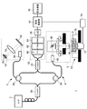
- FIG. 1 is a diagram schematically illustrating a configuration of a viscoelasticity visualization apparatus according to an embodiment.
- the apparatus of the present embodiment visualizes the viscoelasticity of the regenerated tissue by measuring the tomography on a micro scale. For this tomographic measurement, load by acoustic radiation pressure and detection by OCT are used.
- the OCT apparatus 1 includes a light source 2, an object arm 4, a reference arm 6, optical mechanisms 8 and 10, a light detection device 12, a load device 13, a control calculation unit 14, and a display device 16.
- Each optical element is connected to each other by an optical fiber.
- an optical system based on a Mach-Zehnder interferometer is shown, but a Michelson interferometer or other optical system can also be adopted.
- TD-OCT Time Domain OCT
- SS-OCT Sewept Source OCT
- SD-OCT Spectrum Domain OCT
- the light emitted from the light source 2 is divided by a coupler 18 (beam splitter), one of which is guided to the object arm 4 to become object light, and the other is guided to the reference arm 6 to become reference light.
- the object light of the object arm 4 is guided to the optical mechanism 8 via the circulator 20 and is irradiated onto a measurement target (hereinafter referred to as “target S”).
- the target S is a regenerated tissue (cultured tissue) in this embodiment. This object light is reflected as backscattered light on the surface and cross section of the target S, returns to the circulator 20, and is guided to the coupler 22.
- the reference light of the reference arm 6 is guided to the optical mechanism 10 via the circulator 24.
- This reference light is reflected by the reference mirror 26 of the optical mechanism 10, returns to the circulator 24, and is guided to the coupler 22. That is, the object light and the reference light are combined (superimposed) by the coupler 22, and the interference light is detected by the light detection device 12.
- the light detection device 12 detects this as an optical interference signal (a signal indicating the intensity of interference light).
- This optical interference signal is input to the control calculation unit 14 via the A / D converter 28.
- the control calculation unit 14 performs control processing for the entire optical system, control of the load device (ultrasonic vibration device), and image output by OCT.
- the command signal of the control calculation unit 14 is input to the light source 2, the optical mechanisms 8 and 10, the load device 13, and the like via a D / A converter (not shown).
- the control calculation unit 14 processes the optical interference signal input to the light detection device 12 and acquires a tomographic image of the target S by OCT. Based on the tomographic image data, a viscoelastic tomographic distribution in the object S is calculated by a method described later.
- the light source 2 is a broadband light source composed of a super luminescent diode (hereinafter referred to as “SLD”).
- SLD super luminescent diode
- the light emitted from the light source 2 is divided into object light and reference light by the coupler 18 and guided to the object arm 4 and the reference arm 6, respectively.
- a polarization maintaining optical fiber (Polarization Maintaining Fiber) capable of suppressing the influence of polarization is used as an optical fiber.
- the optical mechanism 8 constitutes the object arm 4 and includes a mechanism for guiding the light from the light source 2 to the target S and scanning, and a drive unit for driving the mechanism.
- the optical mechanism 8 includes a collimator lens 40, a biaxial galvanometer mirror 42, and an objective lens 44.
- the objective lens 44 is disposed to face the target S.
- the light that has passed through the circulator 20 is guided to the galvanometer mirror 42 via the collimator lens 40, and is scanned in the x-axis direction and the y-axis direction to irradiate the target S.
- the reflected light from the target S returns to the circulator 20 as object light and is guided to the coupler 22.
- the optical mechanism 10 is an RSOD (Rapid / Scanning / Optical / Delay / Line) mechanism and constitutes a reference arm 6.
- This RSOD may be a single-pass type in which light is irradiated to a diffraction grating 52, which will be described later, once in a reciprocating manner, or a double-pass type in which light is irradiated twice in a reciprocating manner.
- the optical mechanism 10 includes a collimator lens 50, a diffraction grating 52, a lens 54, and a reference mirror 26. The light that has passed through the circulator 24 is guided to the diffraction grating 52 through the collimator lens 50.
- This light is dispersed for each wavelength by the diffraction grating 52 and is condensed by the lens 54 at different positions on the reference mirror 26.
- the reflected light from the reference mirror 26 returns to the circulator 24 as reference light and is guided to the coupler 22. Then, the light is superimposed on the object light and transmitted to the light detection device 12 as interference light.
- the light passing through the diffraction grating 52 may be condensed on the reference mirror 26 by a curved mirror instead of the lens 54.
- the light detection device 12 includes a light detector 60, a filter 62 and an amplifier 64.
- the interference light obtained by passing through the coupler 22 is detected by the photodetector 60 as an optical interference signal.
- the optical interference signal has noise removed or reduced by the filter 62 and is input to the control calculation unit 14 via the amplifier 64 and the A / D converter 28.
- the load device 13 includes a support base 70 for holding the target S on the optical axis of the OCT, an ultrasonic device 72 that outputs ultrasonic waves toward the target S, and a drive circuit 74 that drives the ultrasonic device 72. .
- a support base 70 for holding the target S on the optical axis of the OCT
- an ultrasonic device 72 that outputs ultrasonic waves toward the target S
- a drive circuit 74 that drives the ultrasonic device 72. .
- the drive circuit 74 scans the ultrasonic beam vertically and horizontally so as to synchronize with the detection of the OCT based on a command from the control calculation unit 14.
- the dynamic load vibration load, excitation force
- the acoustic radiation pressure load signal due to this oscillation needs to be amplitude-modulated.
- the amplitude that directly depends on the sound pressure amount (compression load amount) of the acoustic radiation pressure is modulated with a sine wave and transmitted. Since this amplitude modulation promotes tissue deformation, the deformation speed due to this modulation is detected by OCT.
- the control calculation unit 14 includes a CPU, a ROM, a RAM, a hard disk, and the like.
- the control calculation unit 14 performs calculation processing for controlling the entire optical system, driving control of the load device 13, and image output by OCT, using these hardware and software.
- the control calculation unit 14 controls the driving of the load device 13 and the optical mechanisms 8 and 10, processes the optical interference signal output from the light detection device 12 based on the driving, and obtains a tomographic image of the target S by OCT. get. Then, based on the tomographic image data, the viscoelasticity of the tissue in the target S is calculated by a method described later.
- the display device 16 includes, for example, a liquid crystal display, and displays the viscoelasticity of the tissue of the target S calculated by the control calculation unit 14 on the screen in a manner of visualizing the tomography.
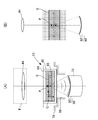
- FIG. 2 is an explanatory diagram illustrating a method of applying a load to the target S without contact.
- A schematically shows the configuration of the load device 13 and its periphery.
- B shows the load state of acoustic radiation pressure.
- the object S is accommodated in a container 80, and the container 80 is set on the support base 70.
- the target S is a regenerated tissue, contamination is not caused during load loading or OCT measurement.
- the container 80 accommodates the substrate 82 seeded with the target S in a state of being immersed in the culture solution C, and is closed (sealed) by a lid 84.
- the container 80, the base material 82, and the lid 84 are made of a material having translucency and sound wave permeability.
- the support base 70 is provided with a vertical through hole 86.
- the container 80 is placed on the support base 70 so as to straddle the through hole 86, and the back surface side is exposed through the through hole 86.
- the object S is arranged so that at least the measurement range is included in the projection plane in the axial direction of the through hole 86.
- the ultrasonic device 72 faces the back surface of the container 80 through the through hole 86 and outputs ultrasonic waves toward the target S.
- the ultrasonic device 72 has a curved transducer array 90 on its upper surface.
- the transducer array 90 includes a plurality of elements 92 arranged in a curved shape.
- the element 92 includes an ultrasonic element (piezo element) that generates ultrasonic waves for vibration.
- the acoustic radiation pressure is focused with the desired position in the target S as the focal point F, and the tissue is focused at the focal point F. It can be vibrated (displaced) (see white arrow).
- a shear wave is generated in the direction parallel to the surface of the object S starting from the focal point F (see a two-dot chain line arrow).
- the light axis by OCT is set to pass through the focal point F of the object S.
- the position of the focal point F can be adjusted (scanned) by selecting (changing) a drive target (energization target) among the plurality of elements 92.
- the ultrasonic radiation elements may be arranged in a planar shape and the acoustic radiation pressure may be focused on the focal point F by using an acoustic lens.
- the control calculation unit 14 sets the focal point F of the acoustic radiation pressure in the target S, the ultrasonic element to be driven, the excitation frequency by the acoustic radiation pressure, and the like, and sends a control signal (pulse) to the drive circuit 74 based on these settings. Output.
- a drive signal (pulse) is output from the drive circuit 74 to the ultrasonic device 72, and an ultrasonic wave (excitation pulse) is output toward the focal point F.
- the control calculation unit 14 can acquire this optical interference signal as a tomographic image of the target S based on the interference light intensity.
- this tomographic distribution can be calculated in three dimensions, the calculation in one or two dimensions will be described here.
- the coherence length l c which is the resolution in the OCT optical axis direction (depth direction) is determined by the autocorrelation function of the light source.
- the coherence length l c is the half-width of the comprehensive line of the autocorrelation function and can be expressed by the following formula (1).
- ⁇ c is the center wavelength of the beam
- ⁇ is the full width at half maximum of the beam.
- the resolution in the direction perpendicular to the optical axis is 1 ⁇ 2 of the beam spot diameter D based on the light condensing performance of the condensing lens.
- the beam spot diameter ⁇ can be expressed by the following formula (2).
- d is a beam diameter incident on the condenser lens
- f is a focal length of the condenser lens.
- the deformation rate distribution of the tissue can be calculated. That is, the electric field E ′ r (t) of the reference light is represented by the following formula (3).
- a (t) is the amplitude
- ⁇ c is the central angular frequency of the light source
- ⁇ r is the Doppler angular frequency generated by the rotation of the RSOD reference mirror 26.
- the electric field E ′ o (t) of the object light is expressed by the following formula (4).
- the detected interference light intensity I ′ d (t) is expressed by the following formula (5).
- the detected tomographic interference signal I d (x, y, z) is expressed by the following equation (6).
- the angular frequency of the interference signal is ⁇ r ⁇ d .
- the Doppler angular frequency shift amount ⁇ d caused by the deformation speed is detected.
- the Doppler angular frequency shift amount omega d it is possible to obtain a deformation speed v.
- lambda c is the center wavelength
- theta (x, y, z) angle formed coordinates (x, y, z) is the incident direction of the deformation rates in the direction of the beam at the light source.
- n is the average refractive index inside the tissue.
- a depth direction (Z-axis direction) scanning method using RSOD is employed.
- the Hilbert transform and the adjacent autocorrelation method are applied. That is, the adjacent autocorrelation method is applied to the analysis signal (complex signal) ⁇ (t) obtained by applying the Hilbert transform to spatially adjacent interference signals.
- the phase difference ⁇ at a predetermined time interval (time difference ⁇ T) in an arbitrary coordinate is obtained, and the Doppler angular frequency shift amount ⁇ d due to the deformation speed is detected.
- the respective interference signals are expressed by the following equation (8).
- s (t) represents the real part of the analytic signal ⁇ (t)
- s ⁇ (t) represents the imaginary part
- ⁇ T represents the acquisition time interval of the j, j + 1-th interference signal
- A represents the amplitude of the interference signal (that is, the backscattering intensity).
- the phase difference between the interference signals is zero.
- the phase difference between the interference signals of ⁇ j and ⁇ j + 1 corresponds to the phase change amount ⁇ d ⁇ T due to Doppler modulation caused by the deformation speed. That is, the Doppler angular frequency shift amount ⁇ d generated by the deformation speed is expressed as the following formula (9).
- the amount of phase change can be detected in the range of ⁇ to ⁇ . Further, by performing an ensemble averaging process on n interference signals according to the following equation (10), the detectability of the Doppler angular frequency shift amount ⁇ d can be improved.
- Doppler angular frequency shift amount omega d obtained as above by substituting the above equation (7) can be calculated deformation velocity v. Based on the deformation speed v, the viscoelasticity of the tissue can be calculated.
- the complex elastic modulus of the viscoelastic body is represented by E * in the following formula (11).
- the real part E ′ of the complex elastic modulus E * corresponds to a component in which stress and strain are in phase
- the imaginary part E ′′ corresponds to a component in which stress and strain are 90 degrees out of phase.
- the former E ′ is an elastic component.
- storage elastic modulus E ′ is an elastic component.
- storage elastic modulus E ′ (hereinafter referred to as “storage elastic modulus E ′”).
- the latter E ′′ corresponds to a viscous component in which the stress and strain rate are in phase and is called “loss elastic modulus” (hereinafter referred to as “loss elastic modulus E” ”). Therefore, the distribution of the storage elastic modulus E ′ and the loss elastic modulus E ′′ can be calculated as a viscoelastic distribution.
- the strain amount (strain rate) at each time can be calculated by the least square method from the distribution of the tissue deformation rate v (distribution in the Z direction), and the amplitude of the strain amount (strain amplitude ⁇ 0) can be detected as a fault.
- the magnitude of the ultrasonic acoustic radiation pressure (stress amplitude ⁇ 0) is a control amount set for the ultrasonic device 72 by the control calculation unit 14, and thus can be grasped.
- the control calculation unit 14 grasps the ultrasonic oscillation timing and the OCT measurement timing, the phase difference (loss angle ⁇ ) between stress and strain can be calculated. Therefore, the storage elastic modulus E ′ and the loss elastic modulus E ′′, which are viscoelastic parameters, can be calculated from the following formula (11), respectively.
- the fault distribution of the storage elastic modulus E ′ and the loss elastic modulus E ′′ obtained in this manner substantially indicates the viscoelastic fault distribution of the tissue.
- the control calculation unit 14 performs the viscoelasticity of the tissue. Visualize the fault.
- This technique is a technique of calculating a deformation vector distribution by applying a digital cross-correlation method to two OCT tomographic images before and after deformation of a measurement object, and detecting a strain rate tensor distribution of the tissue on a micro scale. .
- the recursive cross-correlation method which performs repeated cross-correlation processing.
- This is a technique of applying a cross-correlation method by referring to a deformation vector calculated at a low resolution, limiting an exploration area and hierarchically reducing an inspection area. Thereby, a high-resolution deformation vector can be acquired.
- an adjacent cross-correlation multiplication method (Adjacent cross-correlation Multiplication) that performs multiplication with a correlation value distribution in an adjacent inspection region is used. Then, the maximum correlation value is searched from the correlation value distribution that has been multiplied to increase the SN.
- the sub-pixel accuracy of the deformation vector is important.
- both the up-stream gradient method using brightness gradient (Up-stream Gradientmethod) and the image deformation method considering image expansion and shear (Image Deformation method) are used together to detect deformation vectors with high accuracy.
- the “windward gradient method” here is a kind of gradient method (optical flow method).
- FIG. 3 is a diagram schematically showing a processing procedure by the recursive cross-correlation method.
- FIG. 4 is a diagram schematically showing a processing procedure by subpixel analysis.
- FIGS. 3A to 3C show processing steps by the recursive cross-correlation method. Each figure shows tomographic images before and after continuous imaging by OCT. The previous tomographic image (Image1) is shown on the left side, and the later tomographic image (Image2) is shown on the right side.
- the cross-correlation method is a method for evaluating the local speckle pattern similarity based on the correlation value R ij based on the following equation (12). For this reason, as shown in FIG. 3A, with respect to the preceding and following OCT images, an inspection region S1 to be inspected with similarity to the previous tomographic image (Image1) is set, and the subsequent tomographic image is displayed. In (Image2), a search area S2 that is a search range of similarity is set.
- the Z axis is set in the optical axis direction
- the X axis is set in the direction perpendicular to the optical axis.
- f (X i , Z j ) and g (X i , Z j ) are in the inspection area S1 (N x ⁇ N z pixels) of the center position (X i , Z j ) set in the OCT images before and after the deformation. Represents a speckle pattern. Note that f ⁇ and g ⁇ represent average values of f (X i , Z j ) and g (X i , Z j ) in the inspection region S1.
- a correlation value distribution R i, j ( ⁇ X, ⁇ Z) in the search area S2 (M x ⁇ M z pixels) is calculated, and pattern matching is performed as shown in FIG.
- the movement amount U i, j giving the maximum correlation value is determined as the deformation vector before and after the deformation.
- This method employs a recursive cross-correlation method that increases the spatial resolution by repeating the cross-correlation process while reducing the inspection area S1.
- the spatial resolution is doubled.
- the inspection area S1 is divided into 1 ⁇ 4, and the search area S2 is reduced by referring to the deformation vector calculated in the previous hierarchy.
- the search area S2 is also divided into 1 ⁇ 4.
- Equation (14) is used to set a threshold value using the average deviation ⁇ of a total of nine deformation vectors including the surrounding eight coordinates centered on the coordinates being calculated, and remove the erroneous vectors. Suppresses error propagation associated with recursive processing.
- Um represents the median value of the vector quantity, and the coefficient ⁇ serving as a threshold is arbitrarily set.
- an adjacent cross-correlation multiplication method is introduced as a method for determining an accurate maximum correlation value from a highly random correlation value distribution affected by speckle noise.
- the correlation value distribution Ri, j ( ⁇ x, ⁇ z) in the inspection region S1 and Ri + ⁇ i, j ( ⁇ x, ⁇ z) with respect to the adjacent inspection region overlapping the inspection region S1 Multiplication of Ri, j + ⁇ j ( ⁇ x, ⁇ z) is performed, and a maximum correlation value is retrieved using a new correlation value distribution R′i, j ( ⁇ x, ⁇ z).
- Windward gradient method 4A to 4C show a processing process by subpixel analysis. Each figure shows tomographic images before and after continuous imaging by OCT. The previous tomographic image (Image1) is shown on the left side, and the later tomographic image (Image2) is shown on the right side.
- an upwind gradient method and an image deformation method are used for subpixel analysis.
- the final movement amount is calculated by an image deformation method described later
- the windward gradient method is applied prior to the image deformation method because of the problem of convergence of the calculation.
- the image deformation method and the windward gradient method for detecting the sub-pixel movement amount with high accuracy are applied under the condition of the inspection area size being small and the high spatial resolution.
- the subpixel movement amount is calculated by the windward gradient method.
- the luminance difference before and after deformation at the point of interest is represented by the luminance gradient and movement amount of each component.
- the sub-pixel movement amount can be determined using the least square method from the luminance gradient data in the inspection region S1.
- the windward difference method is used which gives the windward brightness gradient before the subpixel deformation.
- the windward gradient method calculates the movement of the point of interest in the inspection region S1 not only with the pixel accuracy shown in FIG. 4A but also with the sub-pixel accuracy shown in FIG. 4B.
- Each grid in the figure represents one pixel. Actually, it is considerably smaller than the tomographic image shown in the figure, but for the convenience of explanation, it is shown in large size.
- This windward gradient method is a method for formulating the change of the luminance distribution before and after the minute deformation by the luminance gradient and the moving amount.
- f is the luminance
- the following equation (Taylor expansion of the minute deformation f (x + ⁇ x, z + ⁇ z) is performed. 16).
- the above formula (16) indicates that the luminance difference before and after the deformation of the attention point is represented by the luminance gradient and the movement amount before the deformation. Since the movement amount ( ⁇ x, ⁇ z) cannot be determined only by the above equation (16), it is assumed that the movement amount is constant in the inspection region S1, and is calculated by applying the least square method.
- the luminance difference before and after the movement at each point of interest on the right side can only be obtained uniquely. Therefore, how accurately the luminance gradient is calculated is directly related to the accuracy of the movement amount.
- the primary accuracy upwind difference is used. This is because applying high-order differences in differentiating requires a lot of data and is greatly affected when noise is included.
- the high-order difference based on each point in the inspection area S1 uses a lot of data outside the inspection area S1, and there is a problem that the amount of movement of the inspection area S1 itself is lost. is there.
- the difference on the windward side is applied before the deformation.
- the windward is not the actual movement direction but the direction of the subpixel movement amount with respect to the pixel movement amount, and the upwind is determined by performing parabolic approximation on the maximum correlation value peak.
- the luminance difference on the leeward side after the deformation moves in the opposite direction, a difference in luminance at the point of interest occurs, so the difference on the leeward side is applied after the deformation.
- the position of the point of interest before (after) deformation is obtained from the amount of subpixel movement when parabolic approximation is performed.
- the luminance gradient is calculated from the ratio thereof. Specifically, the following formula (17) is used.
- the amount of movement was determined by applying the least square method using the luminance gradient thus calculated and the luminance change.
- the cross-correlation is performed between the inspection region S1 before the tissue deformation and the inspection region S1 in consideration of the expansion and contraction and shear deformation after the tissue deformation, and the sub-pixel deformation amount is determined by iterative calculation based on the correlation value. Note that the expansion and contraction and the shear deformation of the inspection region S1 are linearly approximated.
- the image deformation method is generally used in a material surface strain measurement method, and is applied to an image obtained by photographing a material surface coated with a random pattern with a high spatial resolution camera.
- the OCT tomogram not only contains a lot of speckle noise, but especially in a living tissue, the refractive index changes with the flow of the substrate and water in the tissue, so the deformation to the speckle pattern is large.
- Reduction of the examination area S1 in this method is indispensable for detecting local tissue mechanical characteristics.
- the amount of deformation obtained by the windward gradient method is adopted as the initial value of the convergence calculation, and further, low robustness is realized even when the inspection area S1 is reduced by bicubic function interpolation of the luminance distribution. ing.
- an interpolation function other than bicubic function interpolation may be used.
- a bicubic function interpolation method is applied to the luminance distribution of the OCT tomogram before tissue deformation, and the luminance distribution is made continuous.
- the bicubic function interpolation method is a technique for reproducing spatial continuity of luminance information using a convolution function obtained by piecewise approximating a sinc function.
- a point spread function depending on the optical system is convolved. Therefore, by performing deconvolution using a sinc function, the original continuous luminance distribution is restored.
- the convolution function h (x) is expressed by the following equation (18).
- the value of a is determined based on the verification result by the numerical experiment using the pseudo OCT tomogram.
- the inspection region S1 calculated in consideration of expansion and contraction and shear deformation is accompanied by deformation as it moves.
- the values of x * , z * Is represented by the following formula (19).
- ⁇ x and ⁇ z are distances from the center of the inspection region S1 to the coordinates x and z
- u and v are deformation amounts in the x and z directions, respectively
- ⁇ u / ⁇ x and ⁇ v / ⁇ z are x, respectively.
- the deformation amount in the vertical direction of the inspection region S1 in the z direction, ⁇ u / ⁇ z, and ⁇ v / ⁇ x are the deformation amounts in the shear direction of the inspection region S1 in the x and z directions, respectively.
- the Newton-Raphson method is used for the numerical solution, and the correlation value derivative with 6 variables (u, v, ⁇ u / ⁇ x, ⁇ u / ⁇ z, ⁇ v / ⁇ x, ⁇ v / ⁇ z) is 0. That is, iterative calculation is performed so as to obtain the maximum correlation value.
- the sub-pixel movement amount obtained by the windward gradient method is used as the initial movement amount in the x and z directions.
- the Hessian matrix for the correlation value R is H and the Jacobian vector for the correlation value is ⁇ R
- the update amount ⁇ Pi obtained in one iteration is expressed by the following equation (20).
- the asymptotic solution obtained at any time by iterative calculation is sufficiently small in the vicinity of the convergence solution.
- a correct convergence solution may not be obtained because it cannot be followed by linear deformation.
- the sub-pixel movement amount obtained by the windward gradient method is employed.
- the deformation velocity vector distribution can be calculated by differentiating the deformation vector of subpixel accuracy obtained in this way with respect to time.
- MLSM Moving least square method
- MLSM is a technique that enables smooth calculation of a differential coefficient while smoothing a movement amount distribution.
- the square error equation used in MLSM is expressed by the following equation (21).
- Equation (21) parameters a to k that minimize S (x, z, t) are obtained. That is, the following equation (22) is adopted as a three-variable quadratic polynomial in the horizontal direction x, the depth direction z, and the time direction t as an approximate function. Based on the least square approximation, an optimal derivative is calculated from the following equation (23) and smoothed.
- the strain rate tensor shown in the following formula (24) can be calculated.
- fx and fz indicate the strain increment of each axis, and the strain rate is calculated from the amount of change over time.
- the strain amount can be calculated by time integration of the strain rate calculated by the above equation (24), and the amplitude of the strain amount (strain amplitude ⁇ 0) can be detected as a fault. Further, as described in relation to the above equation (11), the magnitude of the ultrasonic acoustic radiation pressure (stress amplitude ⁇ 0) can be given as the modulation amplitude by the control calculation unit 14 or the drive circuit 74. It is known and the phase difference (loss angle ⁇ ) between stress and strain can also be calculated. Therefore, the storage elastic modulus E ′ and the loss elastic modulus E ′′, which are viscoelastic parameters, can be calculated.
- the fault distribution of the storage elastic modulus E ′ and the loss elastic modulus E ′′ obtained in this way is the viscoelasticity parameter of the tissue.
- the fault distribution will be substantially shown.
- the control calculation unit 14 visualizes the viscoelasticity of the tissue as a tomogram. In addition, formulation is possible even with the strain rate. That is, correspondence with viscoelastic parameters can be taken.
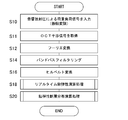
- FIG. 5 is a flowchart showing the flow of the viscoelastic tomographic visualization process executed by the control calculation unit 14. This process is repeatedly executed at a predetermined calculation cycle.
- the control calculation unit 14 drives and controls the light source 2, the optical mechanisms 8 and 10, and the load device 13. Thereby, the acoustic radiation pressure load signal appropriately amplitude-modulated is input to the tissue (S10), and an optical interference signal by OCT is acquired (S11).
- the control calculation unit 14 performs frequency analysis by performing Fourier transform on the optical interference signal for calculation in the frequency space (S12). Subsequently, after the band-pass filtering process is executed so as to correspond to the modulation frequency in the optical mechanism 10 to improve the signal SN ratio (S14), the Hilbert transform is executed (S16). An autocorrelation type real-time viscoelasticity calculation process is executed using the analysis signal obtained by the Hilbert transform (S18). In parallel with this, viscoelastic fault distribution calculation processing is executed (S20).
- the real-time viscoelasticity calculation process is a process of calculating and visualizing the uniaxial (Z direction) viscoelasticity in the tissue of the target S almost in real time in the process of acquiring the OCT tomographic image.
- the viscoelastic tomographic distribution calculation process is a process of acquiring a plurality of OCT tomographic images (two-dimensional images) and visualizing the viscoelasticity of the tissue in a post-process based on them.
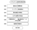
- FIG. 6 is a flowchart showing in detail the real-time viscoelasticity calculation process of S18 in FIG.
- the control calculation unit 14 performs adjacent autocorrelation processing using the analysis signal acquired in S16 to obtain a phase difference at an arbitrary coordinate (S30), and obtains a Doppler frequency (Doppler angular frequency shift amount) (S32).
- the tomographic distribution of the deformation speed in the tissue is calculated by spatial smoothing or spatial averaging processing (S34).
- a strain distribution strain rate distribution
- S36 the least squares method
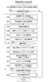
- FIG. 7 is a flowchart showing in detail the viscoelastic fault distribution calculation process of S20 in FIG.
- the control calculation unit 14 calculates the interference light intensity based on the envelope (amplitude) of the analysis signal (S50).
- S50 envelope
- I amplitude
- Is read (S54).
- processing by a recursive cross correlation method is executed.
- cross-correlation processing is executed at the minimum resolution (inspection area of the maximum size) to obtain a correlation coefficient distribution (S56).
- the product of adjacent correlation coefficient distributions is calculated by the adjacent cross correlation multiplication method (S58).
- error vectors are removed by a spatial filter such as a standard deviation filter (S60), and interpolation of the removal vectors is executed by a least square method or the like (S62).
- the cross correlation process is continued by increasing the resolution by reducing the inspection area (S64). That is, the cross-correlation process is executed based on the reference vector at the low resolution. If the resolution at this time is not the predetermined maximum resolution (N in S66), the process returns to S58.
- the processing from S58 to S66 is repeated, and when the cross-correlation processing at the highest resolution is completed (Y in S66), the sub-pixel analysis is executed. That is, based on the distribution of the deformation vector at the maximum resolution (the inspection area of the minimum size), the subpixel movement amount by the windward gradient method is calculated (S68). Based on the sub-pixel movement amount calculated at this time, the sub-pixel deformation amount by the image deformation method is calculated (S70). Subsequently, the error vector is removed by filtering using the maximum cross-correlation value (S72), and interpolation of the removal vector is executed by the least square method or the like (S74).
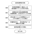
- FIG. 8 is a flowchart showing in detail the viscoelasticity calculation presentation process of S80 in FIG.
- the control calculation unit 6 executes the smoothing of the deformation velocity vector distribution calculated in S76 by the space-time moving least square method (S90). Then, only the component synchronized with the excitation frequency ⁇ (amplitude modulation frequency) by the acoustic radiation pressure is extracted from the smoothed deformation velocity vector (S92). Then, the strain rate tensor is calculated by performing spatial differentiation on the deformation rate vector (S94).
- the strain rate is calculated by time-integrating the strain rate obtained in S94, and the fault distribution of the strain amount (strain amplitude ⁇ 0) is calculated.
- a fault having a storage elastic modulus E ′ and a loss elastic modulus E ′′ using the magnitude of the acoustic radiation pressure of ultrasonic waves (stress amplitude ⁇ 0) and the phase difference between stress and strain (loss angle ⁇ ).
- the distribution is calculated (S96), and the viscoelasticity of the tissue is visualized as a tomogram (S98) It is possible to formulate even with the strain rate, that is, the correspondence with the viscoelastic parameters can be taken.
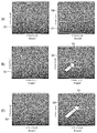
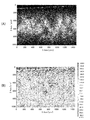
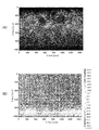
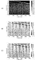
- FIG. 9 and FIG. 10 are diagrams showing experimental results for a sample simulating a biological tissue.
- FIG. 9 shows the results when a hard gel sample is used
- FIG. 10 shows the results when a soft gel sample is used.
- (A) shows an OCT tomographic image
- (B) shows a tomographic distribution of deformation speed (see the above equation (7)).
- the deflection angle of the reference mirror 26 was set to ⁇ 1.9 deg, the scanning frequency was set to 4 kHz, and the depth scanning range (Z direction detection range) of the sample was set to 900 ⁇ m.
- the ultrasonic device 72 was driven with a fundamental wave of 1 MHz, and the applied sound pressure was measured with a hydrophone before the experiment.
- a gel sample (15 mm ⁇ 15 mm ⁇ 5 mm) simulating the optical characteristics of human skin was used.
- Two types of gel samples were prepared: a soft gel sample with a gel hardener weight percentage of 0.5% and a hard gel sample with a weight percentage of the gel hardener four times that of the gel hardener. Visualization evaluation was performed.
- the deformation rate is small in the high-rigid hard gel sample and the deformation rate is large in the low-rigid soft gel sample. This can be said to be in line with the actual situation that the low rigidity portion of the living tissue vibrates greatly (large amplitude) and the high rigidity portion vibrates small (small amplitude) with respect to the excitation force.
- the distribution of the deformation speed in the soft gel sample is due to the distribution of the acoustic radiation pressure.
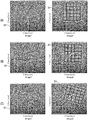
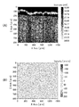
- FIG. 11 and FIG. 12 are diagrams showing experimental results for a layered sample in which the rigidity is changed to a layer.
- FIG. 11 shows the experimental results when no acoustic radiation pressure is applied
- FIG. 12 shows the experimental results when the acoustic radiation pressure is applied.
- (A) shows an OCT tomogram
- (B) shows a tomographic distribution of deformation speed.
- a soft gel layer was used up to about 200 ⁇ m from the surface, and a hard gel layer was used up to about 1000 ⁇ m below it.
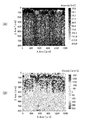
- FIG. 13 is a diagram illustrating experimental results related to viscosity evaluation.
- A shows an OCT tomogram
- B shows a tomographic distribution of deformation speed.
- C shows that there is a phase lag of the deformation speed in the depth direction (Z direction) in (B) by a two-dot chain line.
- a sample similar to that shown in FIG. 12 was used. While performing X-direction scanning in OCT, the amplitude of the acoustic radiation pressure due to ultrasonic waves was periodically changed, and the resulting deformation speed was visualized as a tomogram.
- the amplitude modulation frequency is 2.4 Hz.
- the micro-tomography of the viscoelasticity of the tissue of the target S is visualized by non-contact load loading by acoustic radiation pressure and non-contact / non-invasive tomographic measurement by OCT. For this reason, even if the target S requires strict quality assurance, the contamination can be prevented and the mechanical property evaluation can be performed with high accuracy. This is considered to contribute to the elucidation of biomechanics of regenerative tissues.
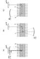
- FIG. 14 is a diagram illustrating a load application method according to a modification.
- A shows a 1st modification
- B shows a 2nd modification
- C shows a 3rd modification.
- the optical mechanism 8 and the ultrasonic device 172 are set on the same side with respect to the target S, and the optical axis by OCT is set to pass through the focal point F.
- the transducer array 190 is formed in a donut shape, and a hole 192 is formed in the center thereof.
- the OCT light is applied to the object S through the hole 192. According to such a structure, it is not necessary to provide a through-hole like the said Example in the support stand of a load apparatus.
- the optical mechanism 8 and the ultrasonic device 72 are arranged on the opposite side with respect to the target S, and the optical axis does not pass through the focus F in the process of tomographic measurement by OCT.
- the case where the focal point F of the ultrasonic device 72 is fixed and OCT X-direction scanning is performed corresponds to this case.
- the deformation of the tissue at a position displaced from the focal point F in the X direction by a predetermined distance is detected.
- the optical mechanism 8 and the ultrasonic device 72 are arranged on the same side with respect to the target S, and the optical axis is set so as not to pass the focal point F in the process of tomographic measurement by OCT. .
- the amplitude and phase of the acoustic radiation pressure can be easily grasped at the detection location by OCT, so that the arithmetic processing becomes easy.
- the accuracy is easy to increase.
- the second and third modified examples have an advantage that the system can be easily constructed.
- the viscoelasticity of the tissue may be determined based on the propagation speed. That is, non-contact elastography based on acoustic radiation pressure may be used to detect tissue viscoelasticity by OCT.
- the support base 70 is fixed, and the optical axis of the OCT and the focal point of the ultrasonic wave are moved.
- the support base 70 may be controlled to move in the X direction and the Y direction, and the ultrasonic focus and the OCT detection position in the target S may be changed.
- the measurement target is a regenerative tissue (cultured cell)
- the above apparatus may be applied to a regenerative treatment of a living body and tissue engraftment may be monitored.
- the apparatus can be applied not only to the medical field such as cartilage diagnosis and skin diagnosis but also to various uses and fields such as the cosmetic surgery field and the cosmetic industry field.
- tissue deformation is induced by acoustic radiation pressure.
- tissue deformation may be induced by incorporating particles having electrical conductivity or magnetism (such as molecular target drugs) into a living tissue and irradiating an electromagnetic field.
- viscoelasticity evaluation is performed from the storage elastic modulus E ′ and the loss elastic modulus E ′′ is shown, but a value expressing the viscoelastic physical quantity is newly added from the storage elastic modulus E ′ and the loss elastic modulus E ′′.
- viscoelasticity evaluation may be performed based on the definition.
- a tomographic image by OCT is acquired in two dimensions, but it may be acquired in three dimensions. That is, not only the depth direction (Z direction) and the X direction but also the Y direction may be scanned to visualize the viscoelasticity of the tissue as a tomographic image.
- this invention is not limited to the said Example and modification, A component can be deform
- Various inventions may be formed by appropriately combining a plurality of constituent elements disclosed in the above-described embodiments and modifications. Moreover, you may delete some components from all the components shown by the said Example and modification.
Abstract
Selon un mode de réalisation, l'invention concerne un dispositif 1 comprenant un système optique utilisant une tomographie par cohérence optique (OCT), et effectuant une visualisation tomographique de la viscoélasticité de tissu dans une cible S. Ce dispositif est équipé: d'un mécanisme optique 8 pour guider et balayer la lumière provenant d'une source lumineuse 2 dans le tissu de la cible S; d'un dispositif de charge 13 pour transmettre une énergie de déformation au tissu; d'une unité de commande et de calcul 14 qui commande l'entraînement du dispositif de charge 13 et du mécanisme optique 8, et, par traitement d'un signal d'interférence optique résultant du système optique au moyen de l'entraînement du dispositif de charge 13 et du mécanisme optique 8, calcule une distribution tomographique de la viscoélasticité du tissu; et d'un dispositif d'affichage 16 qui effectue un affichage de sorte que la viscoélasticité du tissu puisse être visualisée d'une manière tomographique. Le dispositif de charge 13 est un dispositif de charge sans contact qui charge le tissu avec une pression de rayonnement acoustique en émettant des ondes ultrasonores vers un point focal défini à l'intérieur de la cible S.
Priority Applications (2)
| Application Number | Priority Date | Filing Date | Title |
|---|---|---|---|
| JP2019518761A JP7154542B2 (ja) | 2017-05-15 | 2018-05-14 | 組織の粘弾性を断層可視化する装置および方法 |
| US16/685,094 US20200077897A1 (en) | 2017-05-15 | 2019-11-15 | Device and method for tomographically visualizing viscoelasticity of tissue |
Applications Claiming Priority (2)
| Application Number | Priority Date | Filing Date | Title |
|---|---|---|---|
| JP2017-096134 | 2017-05-15 | ||
| JP2017096134 | 2017-05-15 |
Related Child Applications (1)
| Application Number | Title | Priority Date | Filing Date |
|---|---|---|---|
| US16/685,094 Continuation US20200077897A1 (en) | 2017-05-15 | 2019-11-15 | Device and method for tomographically visualizing viscoelasticity of tissue |
Publications (1)
| Publication Number | Publication Date |
|---|---|
| WO2018212115A1 true WO2018212115A1 (fr) | 2018-11-22 |
Family
ID=64273726
Family Applications (1)
| Application Number | Title | Priority Date | Filing Date |
|---|---|---|---|
| PCT/JP2018/018455 WO2018212115A1 (fr) | 2017-05-15 | 2018-05-14 | Dispositif et procédé de visualisation tomographique de la viscoélasticité de tissu |
Country Status (3)
| Country | Link |
|---|---|
| US (1) | US20200077897A1 (fr) |
| JP (1) | JP7154542B2 (fr) |
| WO (1) | WO2018212115A1 (fr) |
Families Citing this family (4)
| Publication number | Priority date | Publication date | Assignee | Title |
|---|---|---|---|---|
| WO2018016652A1 (fr) * | 2016-07-21 | 2018-01-25 | 国立大学法人奈良先端科学技術大学院大学 | Procédé et dispositif de mesure de viscoélasticité |
| JP6979510B2 (ja) * | 2018-02-22 | 2021-12-15 | 富士フイルム株式会社 | 内視鏡システム及びその作動方法 |
| CN110864640A (zh) * | 2018-08-28 | 2020-03-06 | 合肥京东方显示技术有限公司 | 光学系统及利用感光相机测量物体应变的方法 |
| WO2023075694A2 (fr) * | 2021-10-28 | 2023-05-04 | Agency For Science, Technology And Research | Système et procédé de mesure sans contact d'une ou plusieurs propriétés mécaniques d'un matériau |
Citations (6)
| Publication number | Priority date | Publication date | Assignee | Title |
|---|---|---|---|---|
| JP2008510585A (ja) * | 2004-08-24 | 2008-04-10 | ザ ジェネラル ホスピタル コーポレイション | 試料の機械的歪み及び弾性的性質を測定するプロセス、システム及びソフトウェア |
| JP2008170363A (ja) * | 2007-01-15 | 2008-07-24 | Olympus Medical Systems Corp | 被検体情報分析装置、内視鏡装置及び被検体情報分析方法 |
| JP2009507208A (ja) * | 2005-05-27 | 2009-02-19 | ボード オブ リージェンツ, ザ ユニバーシティ オブ テキサス システム | 細胞および組成物の光学コヒーレンス断層撮影法による検出 |
| US20100191110A1 (en) * | 2008-12-01 | 2010-07-29 | Insana Michael F | Techniques to evaluate mechanical properties of a biologic material |
| US20150148654A1 (en) * | 2012-06-29 | 2015-05-28 | The General Hospital Corporation | System, method and computer-accessible medium for providing and/or utilizing optical coherence tomographic vibrography |
| WO2016031697A1 (fr) * | 2014-08-26 | 2016-03-03 | 公立大学法人大阪市立大学 | Dispositif de diagnostic du cartilage et sonde de diagnostic |
Family Cites Families (4)
| Publication number | Priority date | Publication date | Assignee | Title |
|---|---|---|---|---|
| AU2002239360A1 (en) * | 2000-11-28 | 2002-06-11 | Allez Physionix Limited | Systems and methods for making non-invasive physiological assessments |
| JP4646716B2 (ja) * | 2005-02-03 | 2011-03-09 | 三洋電機株式会社 | 微生物検出装置及び微生物検出用カセット |
| DE102009043524A1 (de) * | 2009-09-30 | 2011-03-31 | Siemens Healthcare Diagnostics Products Gmbh | Vorrichtung für die photometrische Untersuchung von Proben |
| WO2011153268A2 (fr) * | 2010-06-01 | 2011-12-08 | The Trustees Of Columbia University In The City Of New York | Dispositifs, procédés et systèmes de mesure des propriétés élastiques de tissus biologiques |
-
2018
- 2018-05-14 JP JP2019518761A patent/JP7154542B2/ja active Active
- 2018-05-14 WO PCT/JP2018/018455 patent/WO2018212115A1/fr active Application Filing
-
2019
- 2019-11-15 US US16/685,094 patent/US20200077897A1/en active Pending
Patent Citations (6)
| Publication number | Priority date | Publication date | Assignee | Title |
|---|---|---|---|---|
| JP2008510585A (ja) * | 2004-08-24 | 2008-04-10 | ザ ジェネラル ホスピタル コーポレイション | 試料の機械的歪み及び弾性的性質を測定するプロセス、システム及びソフトウェア |
| JP2009507208A (ja) * | 2005-05-27 | 2009-02-19 | ボード オブ リージェンツ, ザ ユニバーシティ オブ テキサス システム | 細胞および組成物の光学コヒーレンス断層撮影法による検出 |
| JP2008170363A (ja) * | 2007-01-15 | 2008-07-24 | Olympus Medical Systems Corp | 被検体情報分析装置、内視鏡装置及び被検体情報分析方法 |
| US20100191110A1 (en) * | 2008-12-01 | 2010-07-29 | Insana Michael F | Techniques to evaluate mechanical properties of a biologic material |
| US20150148654A1 (en) * | 2012-06-29 | 2015-05-28 | The General Hospital Corporation | System, method and computer-accessible medium for providing and/or utilizing optical coherence tomographic vibrography |
| WO2016031697A1 (fr) * | 2014-08-26 | 2016-03-03 | 公立大学法人大阪市立大学 | Dispositif de diagnostic du cartilage et sonde de diagnostic |
Non-Patent Citations (2)
| Title |
|---|
| QU, Y. Q. ET AL.: "Acoustic radiation force optical coherence elastography of corneal tissue", IEEE JOURNAL OF SELECTED TOPICS IN QUANTUM ELECTRONICS, vol. 22, no. 3, 25 April 2016 (2016-04-25), pages 1 - 7, XP011607504 * |
| ZHU, J. ET AL.: "Imaging and characterizing shear wave and shear modulus under orthogonal acoustic radiation force excitation using OCT Doppler variance method", OPTICS LETTERS, vol. 40, no. 9, 1 May 2015 (2015-05-01), pages 2099 - 2102, XP055561834 * |
Also Published As
| Publication number | Publication date |
|---|---|
| JPWO2018212115A1 (ja) | 2020-03-12 |
| JP7154542B2 (ja) | 2022-10-18 |
| US20200077897A1 (en) | 2020-03-12 |
Similar Documents
| Publication | Publication Date | Title |
|---|---|---|
| TWI735596B (zh) | 皮膚診斷裝置、皮膚狀態輸出方法、電腦程式產品及記錄媒體 | |
| Song et al. | Tracking mechanical wave propagation within tissue using phase-sensitive optical coherence tomography: motion artifact and its compensation | |
| WO2018212115A1 (fr) | Dispositif et procédé de visualisation tomographique de la viscoélasticité de tissu | |
| Song et al. | Shear modulus imaging by direct visualization of propagating shear waves with phase-sensitive optical coherence tomography | |
| Zvietcovich et al. | Comparative study of shear wave-based elastography techniques in optical coherence tomography | |
| JP5486046B2 (ja) | 変位計測方法及び装置 | |
| JP6707258B2 (ja) | 応力可視化装置および力学物性値可視化装置 | |
| US20150009507A1 (en) | Swept source optical coherence tomography and method for stabilizing phase thereof | |
| KR101704113B1 (ko) | 편광 감응식 광 간섭 단층 촬영의 편광 데이터를 처리하기 위한 방법 및 장치 | |
| JP2010505127A (ja) | 生体環境中での構造および流れの撮像 | |
| US9693728B2 (en) | Systems and methods for measuring mechanical properties of deformable materials | |
| EP2784438B1 (fr) | Procédé pour produire des images bidimensionnelles à partir des données d'interférogramme à tomographie par cohérence optique tridimensionnelle | |
| JP2007152074A (ja) | 変位又は歪計測方法及び装置、速度計測方法、弾性率・粘弾性率計測装置、及び、超音波診断装置 | |
| Neri et al. | Low-speed cameras system for 3D-DIC vibration measurements in the kHz range | |
| Smith et al. | Optimum scan spacing for three-dimensional ultrasound by speckle statistics | |
| JP6623163B2 (ja) | 軟骨診断装置および診断用プローブ | |
| JP6648891B2 (ja) | 物質含有量を断層可視化する装置および方法 | |
| Claus et al. | Large-field-of-view optical elastography using digital image correlation for biological soft tissue investigation | |
| Claeson et al. | Marker-free tracking of facet capsule motion using polarization-sensitive optical coherence tomography | |
| Beuve et al. | Diffuse shear wave spectroscopy for soft tissue viscoelastic characterization | |
| Chen et al. | Quantitative reconstruction of a disturbed ultrasound pressure field in a conventional hydrophone measurement | |
| Almqvist et al. | High resolution light diffraction tomography: nearfield measurements of 10 MHz continuous wave ultrasound | |
| Buchta et al. | Soft tissue elastography via shearing interferometry | |
| JP7174993B2 (ja) | マイクロ断層可視化装置および方法 | |
| Zvietcovich et al. | A comparative study of shear wave speed estimation techniques in optical coherence elastography applications |
Legal Events
| Date | Code | Title | Description |
|---|---|---|---|
| 121 | Ep: the epo has been informed by wipo that ep was designated in this application |
Ref document number: 18802534 Country of ref document: EP Kind code of ref document: A1 |
|
| ENP | Entry into the national phase |
Ref document number: 2019518761 Country of ref document: JP Kind code of ref document: A |
|
| NENP | Non-entry into the national phase |
Ref country code: DE |
|
| 122 | Ep: pct application non-entry in european phase |
Ref document number: 18802534 Country of ref document: EP Kind code of ref document: A1 |