WO2018042840A1 - 連続値最適化問題の大域的探索装置及びプログラム - Google Patents
連続値最適化問題の大域的探索装置及びプログラム Download PDFInfo
- Publication number
- WO2018042840A1 WO2018042840A1 PCT/JP2017/023050 JP2017023050W WO2018042840A1 WO 2018042840 A1 WO2018042840 A1 WO 2018042840A1 JP 2017023050 W JP2017023050 W JP 2017023050W WO 2018042840 A1 WO2018042840 A1 WO 2018042840A1
- Authority
- WO
- WIPO (PCT)
- Prior art keywords
- value
- individuals
- individual
- variable
- evaluation
- Prior art date
- Legal status (The legal status is an assumption and is not a legal conclusion. Google has not performed a legal analysis and makes no representation as to the accuracy of the status listed.)
- Ceased
Links
Images














Classifications
-
- G—PHYSICS
- G05—CONTROLLING; REGULATING
- G05B—CONTROL OR REGULATING SYSTEMS IN GENERAL; FUNCTIONAL ELEMENTS OF SUCH SYSTEMS; MONITORING OR TESTING ARRANGEMENTS FOR SUCH SYSTEMS OR ELEMENTS
- G05B13/00—Adaptive control systems, i.e. systems automatically adjusting themselves to have a performance which is optimum according to some preassigned criterion
- G05B13/02—Adaptive control systems, i.e. systems automatically adjusting themselves to have a performance which is optimum according to some preassigned criterion electric
-
- G—PHYSICS
- G06—COMPUTING OR CALCULATING; COUNTING
- G06N—COMPUTING ARRANGEMENTS BASED ON SPECIFIC COMPUTATIONAL MODELS
- G06N99/00—Subject matter not provided for in other groups of this subclass
Definitions
- This disclosure relates to a global search apparatus and program for continuous value optimization problems.
- Patent Document 1 For example, a method for obtaining an optimum value of a variable, that is, a parameter in a multidimensional search space has been proposed (for example, see Patent Document 1).
- a plurality of individuals whose elements are the parameters for which the optimum value is calculated are generated in the search space, the evaluation values of these individuals are calculated, and the individuals with bad evaluation values are selected from the individuals. Is selected. Then, the selected individual is brought close to an individual having a good evaluation value at a predetermined rate.
- an individual with a bad evaluation value is moved to an arbitrary region within a certain Euclidean distance from the individual with the best evaluation value.
- the purpose of the present disclosure is to search for the minimum or maximum value of an evaluation function having a plurality of extreme values so that the optimal value can be reached with as few times as possible while increasing the probability of reaching the optimal value of the variable.
- an optimization device that derives an individual variable or an optimal value of a variable based on setting an individual in an evaluation function having a plurality of extreme values in a search space having one or more dimensions Is targeted.
- the setting unit sets variables for multiple individuals according to the evaluation function in the search space.
- the extreme value unit derives an attraction potential that causes attraction to act on at least two or more selected individuals among a plurality of individuals set by the setting unit, and adds an evaluation value of an evaluation function by the plurality of individuals
- the effective evaluation value obtained by adding the attractive value between the added value and the derived attractive potential between the selected individuals and multiplying the added value by the attractive force coefficient that acts between the selected individuals is converted into an extreme value.
- the derivation unit changes the variables of the plurality of individuals so that the effective evaluation value is maximized by the extreme value unit while gradually increasing the attractive coefficient from the initial value, and the multiple values when the predetermined end condition is satisfied.
- an individual variable, an optimal value of the variable, an evaluation value corresponding to the variable, or an optimal value of the evaluation value is derived.
- the optimal value can be reached with as few times as possible while increasing the probability of reaching the optimal value of the variable.
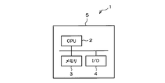
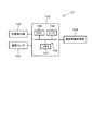
- FIG. 1A is an electrical configuration diagram of a global search device for a continuous value optimization problem according to the first embodiment
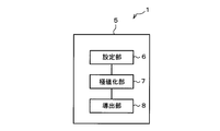
- FIG. 1B is a block diagram functionally illustrating a global search apparatus for a continuous value optimization problem
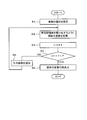
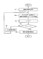
- FIG. 2 is a flowchart schematically showing the flow of processing.
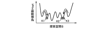
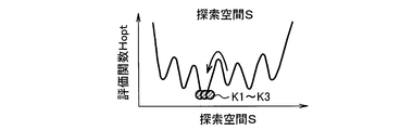
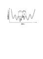
- FIG. 3A is part 1 of an image diagram showing a movement state when an individual converges to an optimal solution in a search space.
- FIG. 3B is part 2 of an image diagram showing a movement state when an individual converges to an optimal solution in the search space.
- FIG. 3A is part 1 of an image diagram showing a movement state when an individual converges to an optimal solution in a search space.
- FIG. 3B is part 2 of an image diagram showing a movement state when an individual converges to an optimal solution in the search space.
- FIG. 3C is part 3 of an image diagram showing a moving state when an individual converges to an optimal solution in the search space.
- FIG. 3D is a fourth part of an image diagram showing a movement state when an individual converges to an optimal solution in the search space;
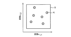
- FIG. 4 is an explanatory diagram of the second embodiment and is a first diagram showing an initial distribution of individuals.
- FIG. 5 is part 2 of the diagram showing the initial distribution of individuals.
- FIG. 6 is part 3 of the diagram showing the initial distribution of individuals.
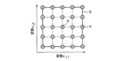
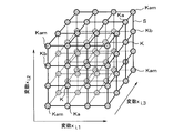
- FIG. 7 is part 4 of the diagram showing the initial distribution of individuals.
- FIG. 8 is part 5 of a diagram showing an initial distribution of individuals,
- FIG. 9 is part 6 of a diagram showing an initial distribution of individuals,
- FIG. 10 is part 7 of a diagram showing an initial distribution of individuals, FIG.
- FIG. 11 is part 8 of the diagram showing the initial distribution of individuals
- FIG. 12 is part 9 of the diagram showing the initial distribution of individuals
- FIG. 13 is part 10 of a diagram showing an initial distribution of individuals
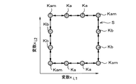
- FIG. 14 is an explanatory diagram of the third embodiment and is a diagram illustrating an example of an individual distribution
- FIG. 15 is an explanatory diagram showing an example of a selected individual that gives an attractive potential
- FIG. 16 is part 2 of an explanatory diagram showing an example of a selected individual that gives an attractive potential
- FIG. 17 is part 3 of an explanatory diagram showing an example of a selected individual that gives an attractive potential
- FIG. 18 is a fourth explanatory diagram showing an example of a selected individual that gives an attractive potential.
- FIG. 15 is an explanatory diagram showing an example of a selected individual that gives an attractive potential
- FIG. 16 is part 2 of an explanatory diagram showing an example of a selected individual that gives an attractive potential
- FIG. 17 is part 3 of an explanatory diagram showing an example of a
- FIG. 19 is part 5 of an explanatory diagram showing an example of a selected individual that gives an attractive potential.
- FIG. 20A is part 1 of an explanatory diagram showing the movement process of an individual
- FIG. 20B is the second part of the explanatory diagram showing the movement process of the individual
- FIG. 20C is a third part of the explanatory diagram showing the movement process of the individual
- FIG. 20D is Part 4 of an explanatory diagram showing the movement process of an individual
- FIG. 21 is an explanatory diagram of the fifth embodiment, schematically illustrating the principle of the auxiliary function method
- FIG. 22 is the first illustration of Lipschitz constants.
- FIG. 23 is the second illustration of Lipschitz constants.
- FIG. 24 is a flowchart schematically showing the flow of processing
- FIG. 25 is a diagram showing an evaluation function used for the simulation.
- FIG. 26 is a diagram showing constants used in the simulation.
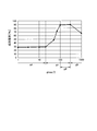
- FIG. 27 shows the simulation result.
- FIG. 28 is a diagram illustrating a process of convergence to a certain predetermined area.
- FIG. 29 is an explanatory diagram of the sixth embodiment and is an explanatory diagram showing a state after the individual has converged,
- FIG. 30 is an electrical configuration diagram showing the seventh embodiment.
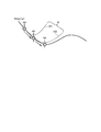
- FIG. 31 is a first part of a bird's eye view showing an optimal route of a moving object at a certain time.
- FIG. 32 is a second bird's-eye view showing the optimum route of the moving object at a certain time.
- the optimization device 1 is a continuous value optimization using a microcomputer (hereinafter referred to as a microcomputer) 5 constituted by connecting a CPU 2, a memory 3 such as a ROM and a RAM, and an input / output interface 4 or a general-purpose computer. Configured as a global search device in question.
- a microcomputer hereinafter referred to as a microcomputer
- the microcomputer 5 executes the optimization process.
- the microcomputer 5 executes an optimization program stored in the memory 3 and executes various procedures to execute an optimization process.
- the memory 3 is used as a non-transitional tangible recording medium.
- the optimization process assumes a search space S composed of Euclidean space having one or more M ( ⁇ 1) dimensions, and the minimum or maximum value of the evaluation function Hopt predetermined in the search space S, that is, process of obtaining the optimal value, or / and, showing the process of obtaining the variable x i to the evaluation function Hopt is the optimum value.
- a form for obtaining the minimum value of the evaluation function Hopt as the optimum value is shown, but it may be applied to processing for obtaining the maximum value as the optimum value.
- the evaluation function Hopt indicates a mathematical function based on one or more M variables (parameters). For example, an arbitrary polynomial, a rational function, an irrational function, an exponential function, a logarithmic function, a combination of addition, subtraction, multiplication and division, etc. Can be mentioned.
- the optimization device 1 includes various functional blocks such as a setting unit 6, an extreme value unit 7, and a derivation unit 8 as functional blocks realized by the microcomputer 5.
- Setting unit 6 sets along the variable x i of a plurality of individual K inside the evaluation function Hopt search space S.
- Each of the plurality of individual K comprises M-dimensional variables x i.
- the extremization unit 7 derives an attractive potential fij that causes an attractive force to act on at least two or more selected individuals K among the plurality of individuals K set by the setting unit 6, and uses the variable x i of the plurality of individuals K.
- An evaluation addition value ⁇ Hopt (x i ) obtained by adding the evaluation value Hopt (x i ) of the evaluation function Hopt and an attractive potential fij between the derived selected individuals K are added, and this added value is added between the selected individuals K.
- the effective evaluation value Heff obtained by adding the attractive force value multiplied by the attractive force coefficient g / 2 to be applied is maximized, and is minimized in the present embodiment.
- the deriving unit 8 increases the variable x i of the plurality of individuals K so that the effective evaluation value Heff is maximized by the extreme value converting unit 7 while gradually increasing the attractive coefficient g / 2 from the initial value (for example, 0).
- the variable x i of the individual K is derived based on the evaluation value of at least one individual K of the plurality of individuals K when the predetermined end condition is satisfied. Then, a plurality of individuals K easily converge to one point of the minimum value of the evaluation function Hopt. In this embodiment, using this principle, a variable x i of a certain individual K is derived and output as a solution.
- FIG. 2 is a flowchart showing the detailed flow of the optimization process
- FIGS. 3A to 3D show image diagrams of the search process.
- the search space S is a one-dimensional Euclidean space
- this evaluation function Hopt is a function having a plurality of minimum values
- the individual K for searching for the minimum value in the evaluation function Hopt The image figure of a movement state is shown.
- the microcomputer 5 sets the individual K along the evaluation function Hopt in S1 of FIG.
- N 3 (N> 2)
- the individuals K1 to K3 will be abbreviated as individuals K, and special individuals K will be described with a suffix after the symbol K. Do.
- the microcomputer 5 obtains the effective evaluation value Heff in S2 of FIG. 2, updates by changing the variables x i of the individual K to minimize the effective evaluation value Heff.
- the effective evaluation value Heff is a value based on the evaluation value Hopt (x i ) obtained by introducing the variable x i of a plurality of individuals K into the evaluation function Hopt as described above, and can be expressed as follows as a specific example. .
- Heff indicates an effective evaluation value
- Hopt (x i ) indicates the evaluation value of each individual K of the evaluation function Hopt.
- g / 2 represents an attractive force coefficient
- ⁇ fij (x i -x j ) represents an added value of the attractive potential.
- the evaluation addition value obtained by adding the evaluation values Hopt (x i ) of the evaluation function Hopt by the plurality of individuals K that is, the variable x i of the plurality of individuals K is substituted into the evaluation function Hopt.
- An addition value obtained by adding the evaluation value Hopt (x i ) is shown, and the second term of the equation (1) adds the attractive potential fij between the plurality of individuals K, and the added value is obtained between the plurality of individuals K.
- the attractive force value obtained by multiplying the attractive force coefficient g / 2 to be applied to is shown.
- the attractive potential fij may be set so that one individual K acts with all other individuals K. However, as shown in an embodiment described later, a part of all the individuals K is used.
- the attractive potential fij may be set by selecting the selected individual K. Further, as the function of the attractive potential fij, as will be described later, a function in which the attractive value increases as the so-called Euclidean distance between a plurality of individuals K increases, or the attractive force regardless of the Euclidean distance may be applied.
- the value may be set to be a constant value. Further, the present invention is not limited to this, and a function in which the attractive value decreases as the Euclidean distance increases may be applied.
- Microcomputer 5 the effective evaluation value Heff obtained by adding the this evaluation sum value and the value of the attractive force derived in S2 in FIG. 2, searches for a variable x i of the individual K to reduce the effective evaluation value Heff. As the search method, it is desirable to use the auxiliary function method shown in the embodiment described later, but any method may be used as long as it is a method capable of searching for extreme values.
- the evaluation function Hopt is a function having a plurality of local minimum values as shown in FIG. 3A
- increasing the attractive coefficient g / 2 of the second term of the equation (1) causes the individual K to converge to one point.
- the individual K rises in order from the lowest mountain, that is, moves so as to exceed the maximum value, and moves in the order of the valley, that is, the minimum value.
- the individual K1 moves the variable x i in the search space S in the direction of increasing example
- individuals K3 is a variable x i in the search space S in a direction to decrease e.g. To do.
- the process for determining whether or not the predetermined upper limit number ⁇ in S4 of FIG. When the state update count t is equal to or smaller than the predetermined upper limit count ⁇ and the termination condition is not satisfied, the microcomputer 5 increases the attractive coefficient g / 2 by, for example, a predetermined number in S5, and returns to S2 to repeat the process.
- the microcomputer 5 repeats the processing of S2 to S3 while gradually increasing the attractive coefficient g / 2 in this way, so that each individual K gradually increases the peak of the maximum value of the evaluation function Hopt as shown in FIG. 3C. It will be over.
- a plurality of individuals K1 to K3 converge to one point of the evaluation function Hopt.
- the microcomputer 5 outputs the solution of the variable x i of any one of the individuals K1 to K3, for example, when the termination condition is satisfied in S5 of FIG. Thereby, the variable x i of the individual K can be output as a solution.
- the attraction coefficient g / 2 to change the variable x i of a plurality of individual K so that the effective evaluation value Heff is extremizing while gradually increasing from the initial value, the state update count t is given
- the variable x i of the individual K is derived based on at least one individual K among the plurality of individuals K when the upper limit number ⁇ is exceeded.
- the variable x i of satisfying individual K evaluation value of the evaluation function Hopt is the lowest may be solution output. This makes it possible to reach the optimum number of times as small as possible while increasing the probability reaching the optimal value of the variable x i.
- (Second Embodiment) 4 to 13 show additional explanatory views of the second embodiment.
- the second embodiment illustrating a method of setting the initial distribution of the variables x i of the individual K.
- each individual K has an M-dimensional variable x i, and the valley of the evaluation function Hopt depends on the form of the initial distribution of the M-dimensional variable x i.
- the number of passes that is, the number of passes of extreme values, and the convergence method also change.
- the microcomputer 5 preferably initializes the individual K so as to fill the search space S in advance. Increasing the number of individuals K increases the accuracy, but increasing the number of individuals K increases the processing time. For this reason, it is desirable to perform processing using a limited number of individuals K, and the initial distribution of the variable x i of the limited number of individuals K occupies an important element in the optimum value search processing. For this purpose, for example, from FIG. 4, as shown in FIG. 13, it is desirable to set the initial distribution of the variables x i of the individual K.
- FIG. 7 shows a plurality of individual individuals K. Shows an example of an initial distribution in a case where M has a three-dimensional variable x i .
- variables x i of a plurality of individuals K may be set in the search space S at random.
- Individuals Ka of FIG Among these, as shown in Kb, may be an upper limit value or lower limit value of at least one or more individuals Ka, the Kb of the variable x i search space S.
- the variable x i of other individual K may be set to random. By setting in this way, a wider range of extreme values can be searched.
- variable x i of the individual K may be set so as to be the lattice point position obtained by dividing the search space S as the initial distribution.
- “adjacent” means the individual K having the shortest Euclidean distance.
- M 3 dimensional variables x i, respectively, as shown in FIG. 7, by setting the variable x i as the individual K is located at the grid point position An initial distribution should be constructed. In this way, by initially distributing the individuals K at the lattice point positions, it is possible to search for the extreme values inside the search space S.
- variable x i of the individual K which contributes to the generation of valleys , is divided by the variable x i, 1 of the individual K having a low contribution degree. May be set larger.
- the degree of contribution is set in advance according to experiments, simulations, or the like, or is set based on qualitative consideration for an actual problem.
- the number of divisions of the variable x i, 2 is 5, and the number of divisions of the variable x i, 1 is 2. Then, it is possible to search for the extreme values in the search space S while reducing the number of individuals K set as the initial distribution. Since the number of individuals K can be reduced, the processing time can be reduced.
- the search space S may be divided into a plurality of partial spaces Sc and Sd as an initial distribution, and an individual K may be set in each of the partial spaces Sc and Sd.
- the effective evaluation value Heff is obtained for each of the partial spaces Sc and Sd
- the variable x i of the individual K is based on at least one individual K of the plurality of individuals K when the effective evaluation value Heff satisfies a predetermined termination condition. May be derived. Thereby, it is possible to exhaustively search the search space S with a smaller number of individuals K.
- subspace Sc it is possible to determine the subspace Sc, obtain the minimum value of the different evaluation functions Hopt every Sd (the optimum value) individual Kg1, Kg2 variables x i, finally subspace Sc, obtained for each Sd individuals Kg1, evaluation value of the evaluation function Hopt variables x i of Kg2 compares, may be derived as a solution to select a variable x i of an individual Kg1, Kg2 to obtain the minimum value of the evaluation value.
- a variable x i changes continuously in time.
- the microcomputer 5 derives a solution of such a variable x i (t) at every predetermined time, in order to obtain a solution of the variable x i (t + 1) at the next timing, the current variable x i (t )
- the derivation process of the solution of the variable x i (t + 1) at the next timing may be performed quickly and accurately.
- a limited search range Sa limited in the search space S is provided as an initial distribution, and the initial distribution is set so as to include the estimated solution xiz as the limited search range Sa. desirable.
- a predetermined range from the estimated solution xiz for example, x i, 1 ⁇ 1 ⁇ variable x i, 1 ⁇ x i, 1 + ⁇ 1, x i, 2 ⁇ 2 ⁇ variable x i, 2 ⁇ x i, 2 + ⁇ 2
- the probability of reaching the optimal solution of the variable x i can be increased with a smaller number of evaluations.
- the initial distribution may be set such that the closer to the space including the estimated solution xiz, the denser the individuals K are distributed, and the further away from the estimated solution, the density of the individuals K is decreased. As a result, the probability of reaching the optimal solution of the variable x i can be increased with a smaller number of individuals K.
- the individuals K are densely distributed within a predetermined range Sb close to the space including the estimated solution xiz as an initial distribution, and other individuals K are randomly distributed outside the predetermined range Sb.
- at least one individual Ka, Kb may be set to the upper limit value or lower limit value of the variable x i of the variable x i a search range S of Kam.
- (Third embodiment) 14 to 20D show additional explanatory diagrams of the third embodiment.
- the attractive potential fij can be expressed as a function of the difference between the i-th individual K and the j-th individual K as shown in the equation (1).
- the attractive potential fij may be obtained by obtaining the difference by the number of combinations of all the two individuals K and obtaining the added value.
- FIG. 14 when many individuals K are densely distributed in one valley H1, and other individuals Kc are sparsely distributed in another valley H2, the density is densely distributed. It becomes easy to be influenced by many individuals K in the valley H1.
- the density of the individual K may vary for each predetermined region and space.
- the attractive potential fij is given to the combination of all two individuals K, the condition that the influence of the density distribution of the individual K is assumed to be strong (for example, the evaluation function Hopt Or / and the condition of the initial distribution of the density of the individual K), it is desirable to select the individual K that gives the attractive potential fij and give the attractive potential fij only between specific selected individuals K.
- the microcomputer 5 orders the identification codes (for example, 1 to 5) in particular for a plurality of individuals K and assigns the identification codes that are adjacent in order.
- the attractive potential fij is derived using the selected individual K as the selected individual K1-K2, K2-K3, K3-K4, K4-K5, and the individual K with the identification code that is not adjacent in order is not selected and the attractive potential fij Should be set to 0. Then, it can converge without making the influence of the density of the individual K too strong.
- FIGS. 15 and 16 show an embodiment in which given the identification codes 1-5 in ascending order of variables x i of the individual K, is necessary to arrange assigned the identification codes 1-5 in ascending order of the variable x i
- the order of attaching the identification codes 1 to 5 does not affect the magnitude of the variable x i .
- the microcomputer 5 derives the attractive potential fij using two adjacent individuals K among these individuals K as selected individuals, and sets the attractive potential fij to 0 without setting the other individuals K as selected individuals.
- the upper limit value variable x i is the search space S or It can be made to converge sequentially from the individual Kam, Ka, Kb which becomes the lower limit value. Then, the search space S can be exhaustively searched.
- FIG. 20A shows the initial distribution. This initial distribution is the same as the initial distribution shown in FIG. 19, but will be described again.
- All individuals K are vertices whose variables x i, 1 and x i, 2 are both the upper limit value or the lower limit value of the search space S.
- the individual Ka and the variable x i, 1 set to the side where the variable xi , 2 is set to the upper limit value or the lower limit value of the search space S are the upper limit value or the lower limit value of the search space S.
- It consists of an individual Kb set on the side. That is, all individuals Ka, Kb, Kam is set such that each two-dimensional variable x i, 1, x i, 2 of one of the variable x i is the upper limit or lower limit.
- two-dimensional variables x i, 1 , x i, 2 are initially set at equal intervals.
- the attractive potential fij is applied with the adjacent individuals Ka, Kb, and Kam as selected individuals.
- the evaluation function Hopt is not taken into consideration is shown.
- the attractive potential fij can be expressed as a function of the difference between the i-th individual K and the j-th individual K, as shown in the equation (1).
- the attractive potential fij is desirably derived based on, for example, the following equation (2) when the p-th variable of the i-th individual K is expressed as xi, p .
- the attraction potential fij in the equation (2) is set so as to increase as the Euclidean distance between the plurality of individuals K increases, and to decrease as the distance between the plurality of individuals K decreases.
- the individuals K distributed over a wide range as the initial distribution can be quickly converged.
- this expression for the differentiable function can be easily extremizing by obtaining the variables x i of the effective evaluation value to the differential value to zero.
- the attractive potential fij may be derived based on the following equation (3), for example.
- (Fifth embodiment) 21 to 26 show additional explanatory views of the fifth embodiment.
- an auxiliary function method as a specific example for changing the variable x i of the individual K so as to minimize the effective evaluation value Heff (x i ) will be described.
- the auxiliary function method is a method used to minimize the evaluation added value of the first term and the attractive value of the second term of the expression (1), and is a quadratic that approximates the evaluation function Hopt to the evaluation function Hopt. It shows a method of replacing with a function and converting it to an extreme value based on the replaced quadratic function.
- FIG. 21 A detailed image of the auxiliary function method is shown in FIG.
- the evaluation function of the variable x is fmej (x)
- the current solution candidate x ⁇ * (xa, xb in FIG. 21) is substituted into the variable x of the evaluation function fmej (x).
- the evaluation value fmej (x ⁇ *) is passed and the differential value is equal to the partial differential value ⁇ fmej (x ⁇ *) / ⁇ x of the evaluation function and includes the solution candidate x ⁇ *.
- a quadratic function ff using a Lipschitz constant L that satisfies a condition for obtaining a value larger than the evaluation value fmej (x i ) in all the variables x i in the space S is introduced.
- This quadratic function ff can be expressed as a right side of equation (4-1). Further, if the solution satisfying the condition that the quadratic function ff becomes an extreme value is xz, it can be derived as shown in the equation (4-2).
- Equation (4-1) L represents a Lipschitz constant
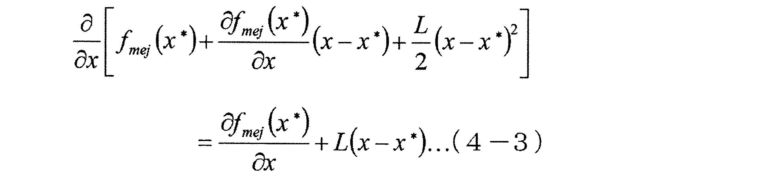
- x ⁇ * represents a current solution candidate for x. If the right side of the equation (4-2) is differentiated, it can be derived as the equation (4-3).
- the second term of the equation (4-3) can be set to 0 by substituting the solution candidate x ⁇ * into the variable x, and the differential value in the current solution candidate x ⁇ * Equals one term.
- the first term of the equation (4-3) coincides with the partial differential value ⁇ fmej (x ⁇ *) / ⁇ x of the evaluation function fmej in the solution candidate x ⁇ *.
- the quadratic function ff is larger than the evaluation value fmej (x i ) of the evaluation function fmej for all variables x i including the solution candidate x ⁇ *. It is desirable to obtain the extreme value of the evaluation function fmej using such a quadratic function ff.
- the solution candidate xz is repeatedly derived.
- the quadratic function ff1 is first searched, and the solution satisfying the extreme value of the quadratic function ff1 is set as the next solution candidate xb.
- the secondary function ff2 is searched again for the next solution candidate xb, and the solution satisfying the extreme value of the quadratic function ff2 is updated to the solution candidate xc.
- the solution candidates change so as to be xa ⁇ xb ⁇ xc.
- equation (2) By substituting the attractive potential fij of equation (2) into equation (1), it can be expressed as the following equation (5). As shown in the fourth embodiment, the function of the attraction potential fij in the equation (5) applies the function of the equation (2) that increases the attraction value when the distance is increased.
- the individual K to which the attractive potential fij is applied as shown in FIG. 15 of the second embodiment, the individual K1-K2, K2-K3,. are selected individuals. That is, a mathematical formula for selecting the i-th and i + 1-th individuals K and applying the attractive potential fij is shown. Although this example will be described here, other examples described in the second and third embodiments can be combined in the same manner.
- the auxiliary function method is applied separately for the first term representing the evaluation function Hopt and the second term representing the attractive coefficient g / 2 ⁇ attractive potential fij.
- the first function on the right side of the equation (5) is replaced by applying the auxiliary function method, the right side of the equation (6) is obtained.
- the right side of the equation (6) shows a mathematical formula in which the auxiliary function method is applied to the first term on the right side of the equation (5) when the q-th variable x j, q in the j-th individual K is updated. Yes. If the second term on the right side of equation (5) is replaced by applying the auxiliary function method, the right side of equation (7) is obtained.
- the Lipschitz constant L should be recalculated every time the solution of the variable x i is updated, and set as small as possible while satisfying the inequality of the equation (4-1).
- the solution x j, q after the update of the q-th variable in the j-th individual in the second term can be derived as in equation (8).
- the qth variable x ⁇ j, q can be updated in the same manner , and the qth variable of the 1st to Nth individuals K can be obtained.
- x j, q can be updated at once using a determinant as shown in equation (9-1).
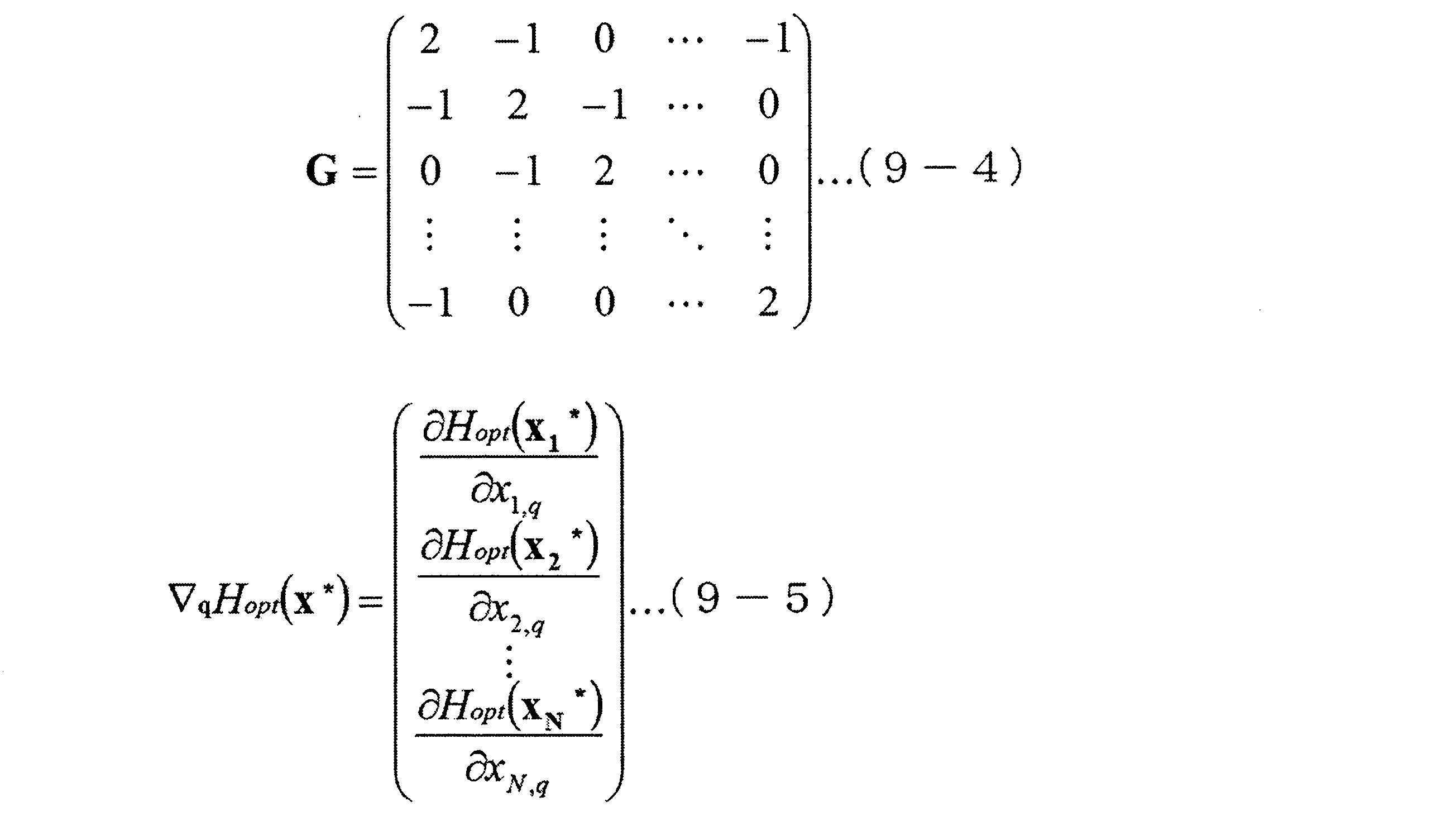
- the variable matrix x q , the Lipschitz coefficient matrix L q , the attractive coefficient matrix G, and the evaluation function partial differentiation matrix q q Hopt are the expressions (9-2), (9-3), (9-4), It can be expressed as shown in equation (9-5).
- the auxiliary function method may be applied to the evaluation function Hopt, and the auxiliary function method may not be used for the attractive value of the second term. That is, when the auxiliary function method is applied only to the evaluation function Hopt when updating the q-th variable x j, q of the j-th individual, the effective evaluation value Heff corresponding to the equations (5) to (7) is (9 -6) It can be expressed as
- the microcomputer 5 first sets a plurality of individuals K in the search space S in S1. At this time, for example, as shown in the second embodiment, an individual K may be set to configure an initial distribution.
- the microcomputer 5 updates all variables x i of the individual K using the equation (8) indicating the auxiliary function method in S2a.
- the processing of S2a may be performed a plurality of times at this timing.
- the microcomputer 5 gradually increases the attractive force value by gradually increasing the attractive coefficient g / 2 between the plurality of individuals K in S5 until a predetermined end condition is satisfied in S4. Then, by repeating these processes of S2a to S5, the individuals K scattered over a wide range converge at one place.
- the timing of increasing the attractive value may be after the update process using the auxiliary function method is executed only once in S2a, or the number of times that the extreme value of the effective evaluation value Heff can be obtained for the process of S2a. It may be after repeated execution.
- the number of individuals K at the end point does not necessarily have to be converged to one predetermined area and converted to an extreme value, but in order to take advantage of the advantage of converging individuals K by attractive force, It is desirable to converge within a predetermined range narrower than the dispersion range of the individual K in the initial distribution.
- the inventor performs a simulation for deriving an optimum value according to an example in which the evaluation function Hopt is a specific mathematical expression.
- the evaluation function Hopt is defined as the following equation (10-1).
- f (x) is the equation (10-2)
- g (x) is the equation (10-3)
- ⁇ is the equation (10-4).
- constants xm, a, P, A, B, C in the expressions (10-1), (10-2), (10-3), and (10-4) are used. Is set.
- the evaluation function Hopt particularly sets the search range (search space S) for the variable x to ⁇ 5.0 ⁇ x ⁇ 5.0.
- search space S search space S
- the predetermined upper limit number ⁇ of the state update count t is set to 100, the number N of individuals K is set to 10, and the process using the auxiliary function method is executed as shown in S2a of FIG. .
- the attractive coefficient g / 2 is increased, but the attractive coefficient g / 2 is increased in accordance with the increase in the number of state updates t as shown in the following equation (10-5). Set to.
- gmax / 2 indicates the maximum value of the attractive coefficient g / 2.
- the horizontal axis represents the maximum value gmax / 2 of the attractive coefficient g / 2
- the vertical axis represents the success probability derived by dividing the number of simulations that can be regarded as successful convergence by the total number of simulations. As shown.
- the success probability depends on gmax / 2.
- the maximum value gmax / 2 of the attractive coefficient g / 2 is made too small, the attractive value is weak and the possibility that the individual K converges becomes low and the success probability becomes relatively low. This method is similar to the so-called parallel gradient method.
- the maximum value gmax / 2 of the attractive coefficient g / 2 is too large, as shown in the range gb of FIG. 27, the evaluation function Hopt is ignored and the probability of success decreases.
- the success probability can be increased as much as possible by setting the maximum value gmax / 2 of the attractive coefficient g / 2 to a certain predetermined range gc which is not the ranges ga and gb.
- a success probability close to 90% could be achieved by setting the maximum value gmax / 2 of the attractive coefficient g / 2 to a specific range gd in the range gc.
- variable x i of the individual K is a predetermined area corresponding to the valley Hy containing an optimal solution in the process of converging to a single point
- the state update count t is shown on the horizontal axis for the state of convergence to xx. As described above, if at least one variable x of the individual after convergence is input to the predetermined region xx shown in FIG.
- FIG. 29 shows an additional explanatory diagram of the sixth embodiment.
- the sixth embodiment shows processing after convergence. For example, even when the process shown in FIG. 2 or FIG. 24 is executed and the effective update value Heff is extreme when the state update count t is repeated up to the predetermined upper limit count ⁇ , as shown in FIG. K does not converge to one point of the valley Hy1 including optimal value, may located Hy2 like other valley, this result can not be determined a variable x i of any of the individual K or solution output There is a case.
- the microcomputer 5 sets the attractive coefficient g / 2 of the second term of the equation (1) to 0 as the final stage process, and derives the extreme value of the evaluation value Hopt of the evaluation function Hopt of the first term as the effective evaluation value Heff. It is desirable to do.
- variable x i of the individual K that satisfies the minimum value of the effective evaluation value Heff obtained by substituting the variable x i into the first term of the equation (1).
- the optimal value of the variable x i can be derived.
- the individual K has not converged in one place, it is possible to reliably obtain the variable x i to the evaluation function Hopt becomes extreme.
- the processing according to the present embodiment is applied, it is not always necessary to converge in one valley (for example, Hy1) when the above-described embodiment or a method combining these embodiments is used, and at least one individual K There become well if the convergence in the valley Hy1, including the optimal solution of the variable x i. Therefore, for example, the predetermined upper limit number ⁇ can be set smaller than in a method not using this process.
- (Seventh embodiment) 30 to 32 show additional explanatory views of the seventh embodiment.
- the seventh embodiment shows an example in which an estimated solution is given in advance before the search is started.
- the vehicle driving support device 101 has been actively developed in recent years to cope with traffic conditions, changes thereof, and accident prevention, and in particular, has been developed to reduce the driving burden on the driver.
- the driving support apparatus 101 includes a controller 102 and is configured by connecting a position detector 103, a speed sensor 104, a map information acquisition unit 105, and the like, and determines an optimal movement position at a future time. It is an apparatus configured as an optimization apparatus that optimizes an optimal route that passes through.
- the controller 102 mainly includes, for example, a CPU 107, a memory 107 such as a ROM, a RAM, and an EEPROM, and a microcomputer 109 having an I / O 108, and a program relating to model prediction control processing is stored in the memory 107.
- the driving support device 101 includes functions as a setting unit 6, an extreme value unit 7, and a derivation unit 8 similar to those in FIG.
- the position detector 103 detects current position information using, for example, GPS (Global Positioning System).
- the speed sensor 104 detects the moving speed of the moving body C.
- the map information acquisition unit 105 acquires map information stored in advance in a predetermined storage device (for example, HDD) or map information from an external map server.
- the controller 102 executes a model prediction control process program stored in the memory 107, thereby acquiring current position information acquired from the position detector 103, movement speed information of the moving object C acquired from the speed sensor 104, And model prediction control is performed based on the map information acquired by the map information acquisition part 105.
- FIG. Various sensors acquired by other sensors such as an ultrasonic sensor for detecting obstacles Ob1 and Ob2 around the vehicle, a distance measuring device for measuring a distance from the obstacles Ob1 and Ob2 around the vehicle, and the like. Model prediction control may be performed using information.
- This model predictive control technology is a technology for performing future prediction, and is a technology for performing optimal control for a certain period including the future and updating these optimal controls at predetermined time intervals.
- the driving support device 101 uses the model predictive control technique to derive an optimal travel route of the moving object (for example, a car) C in a certain period including the future, or to perform predetermined parking without colliding with the obstacles Ob1 and Ob2. Can help lead to space.
- the controller 102 of the driving support apparatus 101 performs the route search process while avoiding the collision with the obstacles Ob1 and Ob2, as shown in the bird's-eye view in FIG. 31, from the current time t0 to the future times t1 to t6.
- the optimum movement position L1 at time t1 is determined by deriving the optimum route R0 of the moving body C in the predetermined period t0 to t6.
- FIG. 32 shows a bird's eye view of the model prediction control process at time t1.
- the controller 102 of the driving support apparatus 101 newly derives the optimum route R1 at future times t2 to t7 after the current time t1 at time t1, but the optimum route R1 at time t1 It can be considered that the locus is close to the optimum route R0 at t0.
- the controller 102 uses, for example, the optimum route R0 based on the positions L1 to L6 corresponding to the times t1 to t6 as an estimated solution, and based on this estimated solution, for example, as shown in the second embodiment, for example, this optimum route R0.
- the initial distribution is configured by setting the individual K so that the individual K is more densely distributed closer to the region including the distance and the density decreases as the distance from the optimum route R0 increases. Then, the probability of reaching the optimal solution with a small number of searches can be increased.
- the controller 102 when the controller 102 derives the optimum route R1 of the moving body C at future times t2 to t7, the past optimum route R0 is used as the estimated solution, and the region including the optimum route R0 as the initial distribution is set. As the distance is closer, the individual K is more densely distributed, and the density of the individual K decreases as the distance from the optimum route R0 increases. Thereby, the probability of reaching the optimal solution with a small number of searches can be increased.
- variable x i of the individual K is output as a solution.
- the evaluation value corresponding to the variable x i that is, the evaluation value obtained by substituting the variable x i to be output as the solution into the evaluation function Hopt. May be output as a solution.
- a variable x i before deducing the attractive force value based on the attractive potential fij to 0 may be derived, and the variable x i may be directly output as a solution.
- the attractive force value may be reduced to 0.
- the optimal value of the variable x i after the conversion may be derived and output as a solution. It is also possible to derived solution output the evaluation values obtained by substituting the optimum values of the variable x i to the evaluation function Hopt. You may apply when deriving such various values.
- the state update count t is conditional on whether exceeds a predetermined upper limit number tau, is not limited thereto, for example, the evaluation value of the evaluation function Hopt of substituting the variable x i is given Different conditions such as whether the value is less than or equal to the value may be used.
- 1 is an optimization device
- 101 is a driving support device (global search device for continuous value optimization problem)
- 102 is a controller
- 6 is a setting unit
- 7 is an extreme value unit
- 8 is a derivation unit
- K denotes an individual
- S is the search space
- x i is a variable
- g / 2 is attraction coefficient
- Hopt evaluation function Heff is an effective evaluation value
- Xiz estimated solution a.
Landscapes
- Engineering & Computer Science (AREA)
- Software Systems (AREA)
- Physics & Mathematics (AREA)
- Theoretical Computer Science (AREA)
- General Physics & Mathematics (AREA)
- Health & Medical Sciences (AREA)
- Mathematical Physics (AREA)
- General Engineering & Computer Science (AREA)
- Computing Systems (AREA)
- Artificial Intelligence (AREA)
- Computer Vision & Pattern Recognition (AREA)
- Evolutionary Computation (AREA)
- Medical Informatics (AREA)
- Automation & Control Theory (AREA)
- Feedback Control In General (AREA)
- Management, Administration, Business Operations System, And Electronic Commerce (AREA)
Abstract
設定部(6)は、複数の個体の変数を探索空間の中の評価関数に沿って設定する。極値化部(7)は、設定部により設定される複数の個体のうち少なくとも2つ以上の選定個体に引力を作用させる引力ポテンシャルを導出し、複数の個体の変数による評価関数の評価値を加算した評価加算値、及び、導出された選定個体の間の引力ポテンシャルを加算しこの加算値に選定個体の間に作用させる引力係数(g/2)とを乗算した引力値、を加算した実効評価値(Heff)を極値化する。導出部(8)は、引力係数を初期値から徐々に大きくしながら極値化部により実効評価値が極値化するように複数の個体の変数を変化させ、所定の終了条件を満たしたときにおける複数の個体の少なくとも一つの個体に基づいて、個体の変数、その変数の最適値、変数に対応した評価値、又は、評価値の最適値による各種値を導出する。
Description
本出願は、2016年9月2日に出願された日本出願番号2016-171776号に基づくもので、ここにその記載内容を援用する。
本開示は、連続値最適化問題の大域的探索装置及びプログラムに関する。
例えば、多次元の探索空間において変数、すなわちパラメータの最適値を求める手法が提案されている(例えば、特許文献1参照)。特許文献1記載の技術によれば、探索空間内に最適値算出対象のパラメータを要素とする複数の個体を生成し、これらの個体の評価値を算出し、個体の中から評価値の悪い個体を選択している。そして、この選択された個体を評価値の良い個体に所定の割合で近づけている。また、評価値の悪い個体を最良の評価値の個体から一定のユークリッド距離内にある任意の領域に移動させている。そして、より良い評価値の個体を選択し最良の評価値の個体を随時更新し、複数の個体の評価値を収束させ、終了判定条件を満たしたと判定した時点で最良の評価値を有する個体に含まれるパラメータをパラメータの最適値として出力している。
特許文献1等に記載の技術を用いて、例えば、複数の極値(例えば、極小値)を備えた評価関数の最小値又は最大値となる変数の最適値を探索するとき、当該変数の最適値への到達確率を高めるためには、複数の個体が最適な1カ所に収束する過程において可能な限り多くの極値(例えば、極小値)を探索することが望ましい。
しかしながら、特許文献1記載の技術を適用したとしても、複数の個体を互いに近づける収束過程において、個体の移動経路はその評価関数の形状とは無関係に決定されてしまう。このため、個体が収束過程において極値を通過するとは限らず、どの個体に収束させることが望ましいか正確に判断できなかったり最適値を通過してしまうことがある。個体の移動処理を極力細かくすることにより最適値への到達確率は高まるものの、個体の移動の回数が増加してしまい好ましくない。
本開示の目的は、複数の極値を備えた評価関数の最小値又は最大値を探索するときに、変数の最適値への到達確率を高めながら極力少ない回数で最適値へ到達できるようにした連続値最適化問題の大域的探索装置及びプログラムを提供することにある。
本開示の一態様によれば、1以上の次元を備えた探索空間に複数の極値を備える評価関数に個体を設定することに基づいて個体の変数又は変数の最適値を導出する最適化装置を対象としている。
設定部は、複数の個体の変数を探索空間の中の評価関数に沿って設定する。また、極値化部は、設定部により設定される複数の個体のうち少なくとも2つ以上の選定個体に引力を作用させる引力ポテンシャルを導出し、複数の個体による評価関数の評価値を加算した評価加算値、及び、導出された選定個体の間の引力ポテンシャルを加算しこの加算値に選定個体の間に作用させる引力係数とを乗算した引力値、を加算した実効評価値を極値化する。そして導出部は、引力係数を初期値から徐々に大きくしながら極値化部により実効評価値が極値化するように複数の個体の変数を変化させ、所定の終了条件を満たしたときにおける複数の個体の少なくとも一つの個体の評価値に基づいて、個体の変数、その変数の最適値、変数に対応した評価値、又は、評価値の最適値を導出する。このような処理を行うことで、複数の極値を備えた評価関数の最小値又は最大値を探索するときに、変数の最適値への到達確率を高めながら極力少ない回数で最適値へ到達できる。
本開示についての上記目的およびその他の目的、特徴や利点は、添付の図面を参照しながら下記の詳細な記述により、より明確になる。図面においては、
図1Aは、第1実施形態を示す連続値最適化問題の大域的探索装置の電気的構成図であり、
図1Bは、連続値最適化問題の大域的探索装置を機能的に示すブロック図であり、
図2は、処理の流れを概略的に示すフローチャートであり、
図3Aは、個体が探索空間内の最適解に収束するときの移動状態を示すイメージ図のその1であり、
図3Bは、個体が探索空間内の最適解に収束するときの移動状態を示すイメージ図のその2であり、
図3Cは、個体が探索空間内の最適解に収束するときの移動状態を示すイメージ図のその3であり、
図3Dは、個体が探索空間内の最適解に収束するときの移動状態を示すイメージ図のその4であり、
図4は、第2実施形態の説明図であり個体の初期分布を示す図のその1であり、
図5は、個体の初期分布を示す図のその2であり、
図6は、個体の初期分布を示す図のその3であり、
図7は、個体の初期分布を示す図のその4であり、
図8は、個体の初期分布を示す図のその5であり、
図9は、個体の初期分布を示す図のその6であり、
図10は、個体の初期分布を示す図のその7であり、
図11は、個体の初期分布を示す図のその8であり、
図12は、個体の初期分布を示す図のその9であり、
図13は、個体の初期分布を示す図のその10であり、
図14は、第3実施形態の説明図であり個体の存在分布の例を示す図であり、
図15は、引力ポテンシャルを与える選定個体の例を示す説明図のその1であり、
図16は、引力ポテンシャルを与える選定個体の例を示す説明図のその2であり、
図17は、引力ポテンシャルを与える選定個体の例を示す説明図のその3であり、
図18は、引力ポテンシャルを与える選定個体の例を示す説明図のその4であり、
図19は、引力ポテンシャルを与える選定個体の例を示す説明図のその5であり、
図20Aは、個体の移動過程を示す説明図のその1であり、
図20Bは、個体の移動過程を示す説明図のその2であり、
図20Cは、個体の移動過程を示す説明図のその3であり、
図20Dは、個体の移動過程を示す説明図のその4であり、
図21は、第5実施形態の説明図であり補助関数法の原理を概略的に示す説明図であり、
図22は、リプシッツ定数の説明図のその1であり、
図23は、リプシッツ定数の説明図のその2であり、
図24は、処理の流れを概略的に示すフローチャートであり、
図25は、シミュレーションに用いた評価関数を示す図であり、
図26は、シミュレーションに用いた定数を示す図であり、
図27は、シミュレーション結果であり、
図28は、ある所定領域に収束する過程を示す図であり、
図29は、第6実施形態の説明図であり個体が収束した後の状態を示す説明図であり、
図30は、第7実施形態を示す電気的構成図であり、
図31は、ある時刻における移動体の最適経路を示す鳥瞰図のその1であり、
図32は、ある時刻における移動体の最適経路を示す鳥瞰図のその2である。
以下、本開示の連続値最適化問題の大域的探索装置及びプログラムの幾つかの実施形態について図面を参照して説明する。以下の実施形態中では、各実施形態間で同一機能または類似機能を備えた部分に同一符号を付して説明を行い、同一又は類似機能を備えた構成及びその作用、連携動作説明等を必要に応じて省略する。
(第1実施形態)
図1A~図3Dは第1実施形態の説明図を示している。最適化装置1は、CPU2と、ROM、RAM等のメモリ3と、入出力インタフェース4とをバス接続して構成されたマイクロコンピュータ(以下マイコン)5、又は汎用コンピュータなどを用いて連続値最適化問題の大域的探索装置として構成される。以下、マイコン5が最適化処理を実行することとして説明を行う。マイコン5が、メモリ3に記憶された最適化プログラムを実行し、各種手順を実行することで最適化処理を実行する。メモリ3は非遷移的実体的記録媒体として用いられる。
図1A~図3Dは第1実施形態の説明図を示している。最適化装置1は、CPU2と、ROM、RAM等のメモリ3と、入出力インタフェース4とをバス接続して構成されたマイクロコンピュータ(以下マイコン)5、又は汎用コンピュータなどを用いて連続値最適化問題の大域的探索装置として構成される。以下、マイコン5が最適化処理を実行することとして説明を行う。マイコン5が、メモリ3に記憶された最適化プログラムを実行し、各種手順を実行することで最適化処理を実行する。メモリ3は非遷移的実体的記録媒体として用いられる。
ここで最適化処理とは、1以上のM(≧1)次元を備えたユークリッド空間からなる探索空間Sを想定し、この探索空間Sに予め定められる評価関数Hoptの最小値又は最大値、すなわち最適値を求める処理、又は/及び、評価関数Hoptが最適値となる変数xiを求める処理を示す。以下では、評価関数Hoptの最小値を最適値として求めるための形態を示すが、最大値を最適値として求める処理に適用しても良い。評価関数Hoptは、1以上のM個の変数(パラメータ)に基づく数式による関数を示すものであり、例えば任意の多項式、有理関数、無理関数、指数関数、対数関数やその加減乗除等による組み合わせなどを挙げることができる。
図1Bに示すように、最適化装置1は、マイコン5により実現される機能ブロックとして、設定部6、極値化部7、及び導出部8などの各種機能ブロックを備えるものである。設定部6は、複数の個体Kの変数xiを探索空間Sの内部の評価関数Hoptに沿って設定する。複数の個体KはそれぞれM次元の変数xiを備える。
また極値化部7は、設定部6により設定された複数の個体Kのうち少なくとも2つ以上の選定個体Kに引力を作用させる引力ポテンシャルfijを導出し、複数の個体Kの変数xiによる評価関数Hoptの評価値Hopt(xi)を加算した評価加算値ΣHopt(xi)、及び、導出された選定個体Kの間の引力ポテンシャルfijを加算しこの加算値に選定個体Kの間に作用させる引力係数g/2とを乗算した引力値、を加算した実効評価値Heffを極値化、本実施形態では極小化する。
そして導出部8は、引力係数g/2を初期値(例えば0)から徐々に大きくしながら極値化部7により実効評価値Heffが極値化するように複数の個体Kの変数xiを変化させ、所定の終了条件を満たしたときにおける複数の個体Kの少なくとも一つの個体Kの評価値に基づいて、個体Kの変数xiを導出する。すると、複数の個体Kが評価関数Hoptの最小値の一点に収束しやすくなる。本実施形態では、この原理を利用し、ある個体Kの変数xiを導出して解出力する。
図2に最適化処理の詳細な流れをフローチャートで示し、図3A~図3Dに探索処理のイメージ図を示している。これらの図3A~図3Dでは、探索空間Sを一次元のユークリッド空間とし、この評価関数Hoptが複数の極小値を備えた関数である場合にその中の最小値を探索する際の個体Kの移動状態のイメージ図を示している。
まずマイコン5は、図2のS1において評価関数Hoptに沿って個体Kを設定する。図3Aには、N=3個(N>2)すなわち複数の個体K1~K3を設定した状態を示している。以下、断らない限り、複数の個体K1~K3のうちの一部又は全ての個体を個体Kと略して説明を行うと共に、特別な個体Kについては符号Kの後に添え字を付して説明を行う。
次に、マイコン5は、図2のS2において実効評価値Heffを求め、この実効評価値Heffを極小化するように個体Kの変数xiを変化させて更新する。実効評価値Heffは、前述したように複数の個体Kの変数xiを評価関数Hoptに導入した評価値Hopt(xi)に基づく値であり、具体例としては下記のように表すことができる。

(1)式の第1項は、複数の個体Kによる評価関数Hoptの評価値Hopt(xi)を加算した評価加算値、すなわち、評価関数Hoptに複数の個体Kの変数xiを代入した評価値Hopt(xi)を加算した加算値を示しており、(1)式の第2項は、複数の個体K間の引力ポテンシャルfijを加算し、この加算値に複数の個体Kの間に作用させる引力係数g/2を乗算した引力値、を示している。この引力ポテンシャルfijは、1つの個体Kが、他の全ての個体Kとの間で作用するように設定しても良いが、後述実施形態に示すように、全ての個体Kのうち一部を選定し当該選定個体Kを対象として引力ポテンシャルfijを設定しても良い。また、この引力ポテンシャルfijの関数は、後述実施形態に示すように、複数の個体K間の所謂ユークリッド距離が遠いほど引力値が大きくなる関数を適用しても良いし、ユークリッド距離に拘わらず引力値が一定値となるように設定しても良い。またこれに限られるものではなく、ユークリッド距離が遠いほど引力値が小さくなる関数を適用しても良い。マイコン5は、図2のS2においてこの評価加算値と引力値とを加算した実効評価値Heffを導出し、実効評価値Heffを小さくする個体Kの変数xiを探索する。この探索方法としては、後述実施形態に示す補助関数法を用いることが望ましいが、極値を探索可能な方法であればどのような方法を用いて探索しても良い。
例えば、評価関数Hoptが図3Aに示すように複数の極小値を備える関数であるときには、(1)式の第2項の引力係数g/2を増加させると、個体Kを一点に収束させる引力が強くなり、個体Kは低い山から順に昇り、すなわち極大値を超えるように順に移動し、谷、すなわち極小値、を順に移動する。このため、例えば図3Bに示すように、個体K1は探索空間S内の変数xiを例えば増加する方向に移動すると共に、個体K3は探索空間S内の変数xiを例えば減少する方向に移動する。
次に、マイコン5は、図2のS3において状態更新回数tをインクリメントすることでt=t+1とし、この状態更新回数tが所定上限回数τを超えたか否か、すなわち図2のS4においてt=τ+1であるか否かを判定する。本実施形態では、この図2のS4における所定上限回数τを超えたか否かの判定処理を所定の終了条件としている。マイコン5は、状態更新回数tが所定上限回数τ以下であり、この終了条件を満たしていないときには、S5において引力係数g/2を例えば所定数だけ増加し、S2に戻り処理を繰り返す。マイコン5は、このように引力係数g/2を徐々に大きくしながらS2~S3の処理を繰り返すことで、図3Cに示すように、各個体Kは評価関数Hoptの極大値の大きな山を徐々に超えるようになる。これらの処理が繰り返されることにより、図3Dに示すように、複数の個体K1~K3が評価関数Hoptの一点に収束するようになる。そして、マイコン5は、図2のS5において終了条件を満たしたときに例えば個体K1~K3のうちの何れか一つの個体Kの変数xiの解を出力する。これにより個体Kの変数xiを解出力できる。
本実施形態によれば、引力係数g/2を初期値から徐々に大きくしながら実効評価値Heffが極値化するように複数の個体Kの変数xiを変化させ、状態更新回数tが所定上限回数τを超えたときにおける複数の個体Kのうち少なくとも一つの個体Kに基づいて個体Kの変数xiを導出している。またこのとき、評価関数Hoptの評価値が最も低くなる条件を満たす個体Kの変数xiを解出力すると良い。これにより、変数xiの最適値への到達確率を高めながら極力少ない回数で最適値へ到達できるようになる。
(第2実施形態)
図4から図13は第2実施形態の追加説明図を示している。第2実施形態では、個体Kの変数xiの初期分布の設定方法を説明する。前述実施形態に示したように、各個体KはM次元の変数xiを備えているが、このM次元の変数xiの初期分布を如何なる形態とするかに応じて、評価関数Hoptの谷の通過数、すなわち極値の通過数、及び、収束方法も変化する。
図4から図13は第2実施形態の追加説明図を示している。第2実施形態では、個体Kの変数xiの初期分布の設定方法を説明する。前述実施形態に示したように、各個体KはM次元の変数xiを備えているが、このM次元の変数xiの初期分布を如何なる形態とするかに応じて、評価関数Hoptの谷の通過数、すなわち極値の通過数、及び、収束方法も変化する。
評価関数Hoptの評価値がどのような値で極値、最小値となるか予め把握することはできないため、マイコン5は、予め探索空間Sを満たすように個体Kを初期設定することが望ましい。個体Kの数を多くすれば精度が高くなるが、個体Kの数を多くすれば処理時間も大きくなる。このため、限られた数の個体Kを用いて処理を行うことが望ましく、この限られた個体Kの変数xiの初期分布が最適値の探索処理に重要な要素を占めることになる。このためには、例えば図4から図13に示すように、個体Kの変数xiの初期分布を設定することが望ましい。
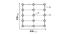
図4から図6、図8から図13は、複数のそれぞれの個体KがM=2次元の変数xiを備えている場合の初期分布の例を示し、図7は複数のそれぞれの個体KがM=3次元の変数xiを備えている場合の初期分布の例を示している。
M=2次元の探索空間Sを想定したときに、例えば図4に示すように、探索空間S内に複数の個体Kの変数xiをランダムに設定すると良い。この場合、個体Kが一点に収束する過程において広範囲の極値を探索することができるようになる。この中でも図5の個体Ka、Kbに示すように、少なくとも1つ以上の個体Ka、Kbの変数xiを探索空間Sの上限値又は下限値とすると良い。また、その他の個体Kの変数xiをランダムに設定すると良い。このように設定することで、さらに広範囲の極値を探索できる。特に、探索空間Sの中で全ての変数xiについて上限値又は下限値となるように個体Kamの変数xiを設定することがさらに望ましい。
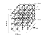
また、例えば図6に示すように、初期分布として探索空間Sを分割した格子点位置になるように個体Kの変数xiを設定しても良い。この場合、図6にM=2次元の例を示すように、隣接する個体Kの間を等分割して設定しても良いが、変数xi毎、すなわちxi,1、xi,2毎に異なる分割数となるように設定しても良い。ここで「隣接」とはユークリッド距離が最も近い個体Kを意味する。また、例えば、複数の個体KがそれぞれM=3次元の変数xiを備えているときには、図7に示すように、個体Kが格子点位置に位置するように変数xiを設定することで初期分布を構成すると良い。このように格子点位置に個体Kを初期分布させることで探索空間Sの内部における極値を網羅して探索できる。
さらに図8に示すように、個体Kの変数xiが谷の生成に寄与する寄与度の高い個体Kの変数xi,2の分割数を寄与度の低い個体Kの変数xi,1よりも大きく設定するようにしても良い。寄与度は、予め実験やシミュレーション等に応じて設定したり、実際の問題に対する定性的な考察から設定する。図8の例では、変数xi,2の分割数を5とし、変数xi,1の分割数を2としている。すると、初期分布として設定する個体Kの数を削減しながら探索空間Sの内部における極値を網羅して探索できる。個体Kの数を削減できるため処理時間を削減できる。
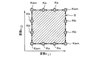
また図9に示すように、例えば図6から図8のように設定されている場合、この中から少なくとも1つ以上の変数xiが探索空間Sで上限値又は下限値となる個体Kだけを選定して設定しても良い。すると、個体Kの数を削減しながら広範囲において極値の探索を行うことができる。
また図10に示すように、初期分布として探索空間Sを複数の部分空間Sc、Sdに分けて各部分空間Sc、Sdにそれぞれ個体Kを設定しても良い。このとき、各部分空間Sc、Sd毎に実効評価値Heffを求め当該実効評価値Heffが所定終了条件を満たしたときにおける複数の個体Kの少なくとも一つの個体Kに基づいて個体Kの変数xiを導出するようにしても良い。これにより、より少ない個体Kの数で探索空間Sを網羅的に探索できる。この場合、部分空間Sc、Sd毎に異なる評価関数Hoptの最小値(最適値)を得る個体Kg1,Kg2の変数xiを求めることができるが、最終的に部分空間Sc、Sd毎に得られた個体Kg1,Kg2の変数xiの評価関数Hoptの評価値を比較し、この評価値の最小値を得る個体Kg1,Kg2の変数xiを選定して解として導出すると良い。
これまで説明したように、収束過程において広範囲の極値を探索できるようにするため、探索空間Sの全てを極力網羅するように個体Kを広範囲に分布させることが望ましいが、例えば探索空間Sの内部に推定解が与えられる場合もある。
例えば、ある変数xiが時間的に連続して変化することを考慮する。例えばマイコン5がこのような変数xi(t)の解をある所定の時間毎に導出するときに、次回のタイミングにおける変数xi(t+1)の解を得るために今回の変数xi(t)の解を推定解xizとして与えることで、次回のタイミングにおける変数xi(t+1)の解の導出処理を素早くしかも正確に行うことができる場合もある。
このような場合、図11に示すように、初期分布として探索空間S内に限定された限定探索範囲Saを設け、この限定探索範囲Saとして推定解xizを含むように初期分布を設定することが望ましい。特にこの場合、例えば推定解xizから所定範囲(例えばxi,1-α1<変数xi,1<xi,1+β1、xi,2-α2<変数xi,2<xi,2+β2;但し、α1、α2、β1、β2>0)を満たすように限定探索範囲Saを絞ることが望ましい。これにより、さらに少ない評価回数で変数xiの最適解への到達確率を高めることができる。
さらに図12に示すように、初期分布として推定解xizを含む空間に近いほど個体Kを密に分布させると共に推定解から遠ざかるほど個体Kの密度を減少させるように設定するようにしても良い。これにより、より少ない個体Kの数で変数xiの最適解への到達確率を高めることができる。
さらに図13に示すように、初期分布として推定解xizを含む空間に近い所定範囲Sb内に個体Kを密に分布させると共にその他の個体Kを所定範囲Sbの外にランダムに分布させ、その他の個体Kのうち、少なくとも1つの個体Ka、Kb、Kamの変数xiを探索範囲Sの変数xiの上限値又は下限値に設定するようにしても良い。これにより、変数xiの推定解xizの付近を重点的に探索しながら広範囲を探索することができ、推定解xiz又はその周辺に解が存在していなかった場合においても、変数xiの最適解への到達確率の低下を防ぐことができる。
(第3実施形態)
図14から図20Dは第3実施形態の追加説明図を示す。第3実施形態は、選定個体の選定方法について説明する。引力ポテンシャルfijは(1)式に示したように、i番目の個体Kとj番目の個体Kの差の関数として表すことができる。この場合、引力ポテンシャルfijは、全ての2つの個体Kの組み合わせ数分の差分を求めて加算値を求めるようにすると良い。しかし図14に示すように、多数の個体Kが一の谷H1の中で密に分布すると共に、他の個体Kcが他の谷H2の中で疎に分布しているときには、密度が密に分布している谷H1の中の多数の個体Kの影響を受けやすくなる。
図14から図20Dは第3実施形態の追加説明図を示す。第3実施形態は、選定個体の選定方法について説明する。引力ポテンシャルfijは(1)式に示したように、i番目の個体Kとj番目の個体Kの差の関数として表すことができる。この場合、引力ポテンシャルfijは、全ての2つの個体Kの組み合わせ数分の差分を求めて加算値を求めるようにすると良い。しかし図14に示すように、多数の個体Kが一の谷H1の中で密に分布すると共に、他の個体Kcが他の谷H2の中で疎に分布しているときには、密度が密に分布している谷H1の中の多数の個体Kの影響を受けやすくなる。
すると、図14の矢印Yに示すように、本来評価値が最小値となり変数xiが最適値となる個体Kcが、他の多数の個体Kの影響を受けて谷H2を抜け出してしまうことがある。また例えば第2実施形態に初期分布を示したように、個体Kの密度がそのある所定の領域、空間毎にばらつくこともある。
このような場合を考慮し、全ての2つの個体Kの組み合わせに引力ポテンシャルfijを与えてしまうと、個体Kの密度分布の影響が強くなることが想定されるような条件(例えば、評価関数Hoptの条件、又は/及び、個体Kの密度の初期分布の条件)を用いるときには、引力ポテンシャルfijを与える個体Kを選定し、特定の選定個体Kの間にだけ引力ポテンシャルfijを与えることが望ましい。
この場合、図15に変数M=1次元の例を示すように、マイコン5が特に複数の個体Kに対し識別符号(例えば1~5)を順序付けて付し、順序が隣接する識別符号が付された個体Kを選定個体K1-K2、K2-K3、K3-K4、K4-K5として引力ポテンシャルfijを導出し、順序が隣接しない識別符号が付された個体Kを選定個体とせず引力ポテンシャルfijを0とすると良い。すると個体Kの密度の影響を強くしすぎることなく収束させることができる。
また、マイコン5が全個体Kに対し引力ポテンシャルfijを対等に印加するためには、図16に示すように、個体K1と個体K5との間にも引力ポテンシャルfijを印加するようにすると良い。なお図15及び図16には個体Kの変数xiの小さい順に識別符号1~5を付した形態を示しているが、変数xiの小さい順に識別符号1~5を付して並べる必要はなく、識別符号1~5を付す順序は変数xiの大小に影響するものではない。
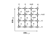
また図17にM=2次元の選定個体Kの例を示す。この図17は図6のように探索空間SにおけるM=2次元の格子点位置に個体Kを初期分布させたときの選定個体の例を示す。また図18に変数M=3次元の例を示す。この図18は図7のようにM=3次元の格子点位置に個体Kを初期分布させたときの選定個体の例を示す。
マイコン5は、格子点位置の個体Kと隣接する格子点位置の最大2×M個の個体Kを選定個体として引力ポテンシャルfijを導出し、その他の個体Kを選定個体とせず引力ポテンシャルfijを0とすることが望ましい。図17に示すように、個体Kd1に隣接する格子点位置に存在する個体Kd2~Kd5を選定個体として引力ポテンシャルfijを設定し、その他の個体Kを選定個体としないように引力ポテンシャルfijを0に設定する。すなわち、個体KがそれぞれM=2次元の変数xiを備えるときには、最大2×M=4個の隣接する格子点位置の個体Kを選定個体として引力ポテンシャルfijを導出する。
また、図18に示すように、個体KがそれぞれM=3次元の変数xiを備えるときには、最大2×M=6個の格子点位置の個体Kを選定個体として引力ポテンシャルfijを導出する。
また図19には図9に示すようにM=2次元の格子点位置の上限値又は下限値に個体Kを初期分布させたときの選定個体Kの例を示す。マイコン5は、これらの個体Kのうち隣接する2個の個体Kを選定個体として引力ポテンシャルfijを導出し、その他の個体Kを選定個体とせず引力ポテンシャルfijを0とする。図19に示すように、マイコン5が例えば初期分布として複数の個体Kを探索範囲Sの変数xiの上限値又は下限値に設定した場合には、探索空間Sにおいて変数xiが上限値又は下限値となる個体Kam、Ka、Kbから順次収束させることができる。すると探索空間Sを網羅して探索できる。
<評価関数Hoptを考慮しない場合における初期分布からの個体Kの移動イメージ>
図20Aから図20Dに個体Kの移動イメージを示している。図20Aに初期分布を示している。この初期分布は、図19に示す初期分布と同様であるが、改めて説明すると、全個体Kは、変数xi,1及びxi,2が共に探索空間Sの上限値又は下限値となる頂点に設定された個体Kam、変数xi,2が探索空間Sの上限値又は下限値となる辺部に設定された個体Ka、変数xi,1が探索空間Sの上限値又は下限値となる辺部に設定された個体Kb、からなっている。すなわち、全個体Ka、Kb、Kamは、それぞれ2次元の変数xi、1、xi、2の何れかの変数xiが上限値又は下限値となるように設定されている。
図20Aから図20Dに個体Kの移動イメージを示している。図20Aに初期分布を示している。この初期分布は、図19に示す初期分布と同様であるが、改めて説明すると、全個体Kは、変数xi,1及びxi,2が共に探索空間Sの上限値又は下限値となる頂点に設定された個体Kam、変数xi,2が探索空間Sの上限値又は下限値となる辺部に設定された個体Ka、変数xi,1が探索空間Sの上限値又は下限値となる辺部に設定された個体Kb、からなっている。すなわち、全個体Ka、Kb、Kamは、それぞれ2次元の変数xi、1、xi、2の何れかの変数xiが上限値又は下限値となるように設定されている。
隣接する個体Kは、2次元の変数xi、1、xi、2が等間隔で初期設定されている。そして、この例では、隣接する個体Ka、Kb、Kamを選定個体として引力ポテンシャルfijを印加するようにしている。なお、説明を単純化するため評価関数Hoptは考慮しない例を示す。
この例の場合、矢印を付した隣接した選定個体Ka、Kb、Kamの間に引力がかかるため、隣接する個体Ka、Kb、Kamは当該引力を合成したベクトル方向に引き寄せられることになる。このため、まず図20Bに示すように、探索空間Sの頂点に初期設定された個体Kamが、探索空間Sの内方に引き込まれるように移動する。さらに図20Cに示すように、探索空間Sの辺部に初期設定された個体Ka、Kbが探索空間Sの内方に引き込まれるように移動する。
さらに図20Dに示すように、全個体Ka、Kb、Kamが徐々に探索空間Sの中央内側に引き込まれるように移動する。これにより全個体Ka、Kb、Kamがそれらの2変数xi,1、xi,2が互いに同一となる一点に収束するようになる。この例では、評価関数Hoptを考慮していない例を挙げているため、最終的には探索空間Sの中央に収束することになるが、実際に評価関数Hoptを考慮すれば、変数xiに応じた評価値Hopt(xi)が実効評価値Heffに反映されるため、この実効評価値Heffを最小化するように個体Ka、Kb、Kamが移動する。すなわち個体Ka、Kb、Kamのそれぞれの変数xiが変化する。これにより、これらの全探索空間Sにおいて変数xiの最適値を網羅的に探索できることがわかる。
(第4実施形態)
以下、第4実施形態を説明する。この第4実施形態では、引力ポテンシャルfijの設定方法について説明する。引力ポテンシャルfijは(1)式に示したように、i番目の個体Kとj番目の個体Kの差分の関数として表すことができる。この場合、引力ポテンシャルfijは、i番目の個体Kのp番目の変数をxi,pと表したときに、例えば下記の(2)式に基づいて導出することが望ましい。
以下、第4実施形態を説明する。この第4実施形態では、引力ポテンシャルfijの設定方法について説明する。引力ポテンシャルfijは(1)式に示したように、i番目の個体Kとj番目の個体Kの差分の関数として表すことができる。この場合、引力ポテンシャルfijは、i番目の個体Kのp番目の変数をxi,pと表したときに、例えば下記の(2)式に基づいて導出することが望ましい。

また、引力ポテンシャルfijを例えば下記の(3)式に基づいて導出するようにしても良い。

(第5実施形態)
図21~図26は第5実施形態の追加説明図を示す。本実施形態では、実効評価値Heff(xi)を極小化するように個体Kの変数xiを変化させるための具体例となる補助関数法について説明する。補助関数法は、(1)式の第1項の評価加算値、第2項の引力値を極小化するときに用いられる一方法であり、評価関数Hoptを当該評価関数Hoptに近似した2次関数に置換し、この置換した2次関数に基づいて極値化する方法を示している。
図21~図26は第5実施形態の追加説明図を示す。本実施形態では、実効評価値Heff(xi)を極小化するように個体Kの変数xiを変化させるための具体例となる補助関数法について説明する。補助関数法は、(1)式の第1項の評価加算値、第2項の引力値を極小化するときに用いられる一方法であり、評価関数Hoptを当該評価関数Hoptに近似した2次関数に置換し、この置換した2次関数に基づいて極値化する方法を示している。
以下、補助関数法について詳細説明する。補助関数法の詳細イメージを図21に示している。図21に示すように、変数xの評価関数をfmej(x)としたときに、この評価関数fmej(x)の変数xに現在の解候補x^*(図21ではxa、xb)を代入し、この評価値fmej(x^*)を通過すると共に、その微分値が評価関数の偏微分値∂fmej(x^*)/∂xと等しく、且つ、その解候補x^*を含む探索空間S内の全ての変数xiにおける評価値fmej(xi)よりも大きな値を得る条件を満たすリプシッツ定数Lを用いた2次関数ffを導入する。この2次関数ffを数式化すると、(4-1)式の右辺のように示すことができる。また、この2次関数ffが極値となる条件を満たす解をxzとすると(4-2)式のように導出できる。

(4-2)式に示すように、解候補xzを繰り返し導出する。図21に示すように、現在の解候補をxaとしたときに、まず2次関数ff1を探索し、2次関数ff1の極値を満たす解を次回の解候補xbとする。その後、この次回の解候補xbについて再度2次関数ff2の探索を行い、2次関数ff2の極値を満たす解を解候補xcに更新する。したがって解候補はxa→xb→xcとなるように変化する。これらの処理が、例えば所定回数以上繰り返されることで評価関数fmej(x)の極小値と見做すことが可能な解(例えばxc)を得ることができる。
さて(1)式に(2)式の引力ポテンシャルfijを代入すると下記の(5)式のように示すことができる。この(5)式における引力ポテンシャルfijの関数は、第4実施形態に示したように、距離を大きくしたときに引力値を大きくする(2)式の関数を適用している。

この(5)式の右辺において、評価関数Hoptを表す第1項と、引力係数g/2×引力ポテンシャルfijを表す第2項とに分けて補助関数法を適用する。(5)式の右辺の第1項について、補助関数法を適用して置換すると(6)式の右辺のようになる。


リプシッツ定数Lは大きすぎると、(4-1)式の不等式を満たすことになるものの、2次係数が比較的大きくなることから、図22に2次関数ffのイメージを示すように、解の更新処理の幅が小さくなりすぎる。このため、評価関数Hoptの谷H2の極値に到達するまでの処理ステップが多くなり処理時間が長くなる。
逆に、リプシッツ定数Lが小さすぎると(4-2)式の不等式を満たさなくなり、図23に2次関数ffのイメージを示すように、解の更新処理の幅が大きくなりすぎる。すると、1ステップの処理だけで隣接する谷H1に移動してしまうことが確認されている。
このため、リプシッツ定数Lは、変数xiの解を更新する度に計算し直すと共に、式(4-1)の不等式を満たす中で可能な限り小さい値を設定すると良いが、特に(5)式の右辺の第2項に補助関数法を適用するときには、(7)式に示すようにリプシッツ係数Lを4に固定することが望ましい。このリプシッツ係数L=4は変数xiの解を更新処理する度に導出し直す必要がないことが発明者らにより確認されている。このとき特に、第2項におけるj番目の個体におけるq番目の変数の更新後の解xj,qは(8)式のように導出できる。



また、評価関数Hoptに補助関数法を適用し、第2項の引力値に補助関数法を用いなくても良い。すなわち、j番目の個体のq番目の変数xj,qを更新するときに評価関数Hoptだけに補助関数法を適用すると、(5)~(7)式に対応した実効評価値Heffは(9-6)式のように表すことができる。




このような最適化処理のフローチャートを図24に示している。図24に示すように、マイコン5はまずS1において探索空間S内に複数の個体Kを設定する。このとき、例えば第2実施形態に示したように個体Kを設定して初期分布を構成すると良い。マイコン5は、引力係数g/2を初期値=0とすることで実効評価値Heff=(1)式の右辺の第1項(=複数の個体Kの評価関数Hoptの評価値)となるように初期設定する。そして、マイコン5はS2aにおいて補助関数法を示す(8)式を用いて個体Kの全変数xiを更新する。
このS2aの処理は、このタイミングで複数回行うようにしても良い。そして、マイコン5は、S4にて所定の終了条件を満たすまで、S5において複数の個体Kの間の引力係数g/2を徐々に増加させることで引力値を徐々に強くする。すると、これらのS2a~S5の処理を繰り返すことで広範囲に散らばった個体Kは1カ所に収束することになる。引力値を増加するタイミングは、S2aにおいて補助関数法を用いた更新処理を1回だけ実行した後でも良いし、S2aの処理について実効評価値Heffの極値を得られることが想定される回数だけ繰り返し実行した後であっても良い。
また、終了時点における個体Kの数は必ずしも1カ所の所定領域に収束して極値化している必要はないものの、引力により個体Kを収束させることによる優位性を活用するために、処理後には初期分布における個体Kの分散範囲よりも狭い所定範囲内に収束していることが望ましい。
<具体例>
発明者は評価関数Hoptを具体的な数式とした実例に合わせて最適値を導出するシミュレーションを行っている。以下ではこの具体例を説明する。評価関数Hoptを下記の(10-1)式と定義した。ただし、f(x)は(10-2)式、g(x)は(10-3)式とし、ωは(10-4)式としている。
発明者は評価関数Hoptを具体的な数式とした実例に合わせて最適値を導出するシミュレーションを行っている。以下ではこの具体例を説明する。評価関数Hoptを下記の(10-1)式と定義した。ただし、f(x)は(10-2)式、g(x)は(10-3)式とし、ωは(10-4)式としている。
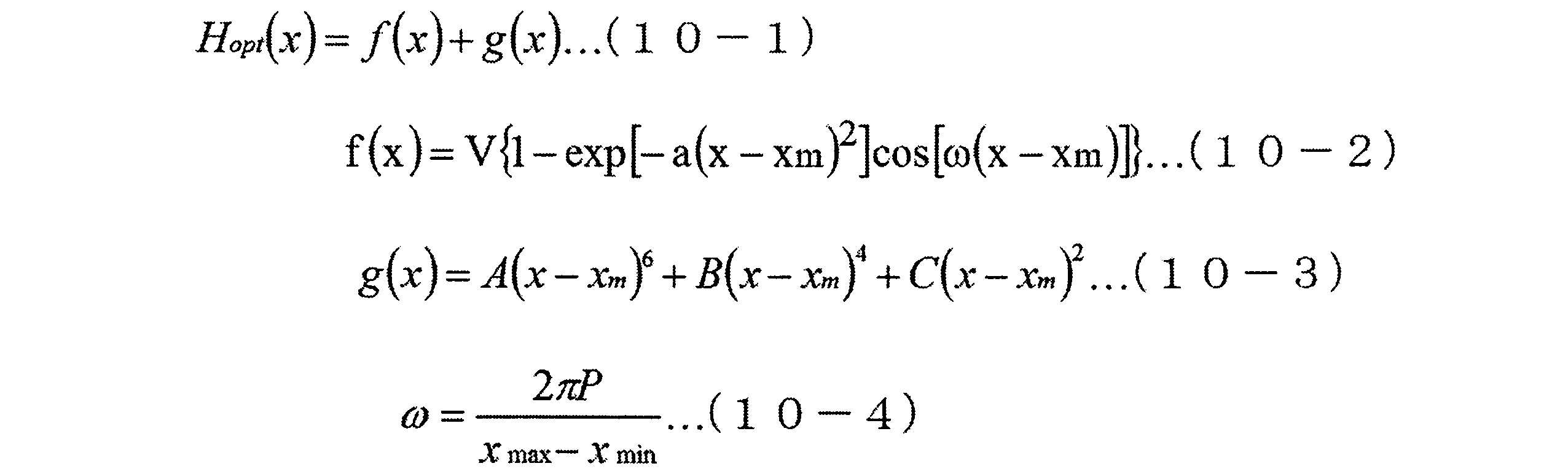
また図26に示したように、状態更新回数tの所定上限回数τを100とし、個体Kの数Nを10とし、図24のS2aに示すように、補助関数法を適用した処理を実行した。また図24の処理ステップS5において、引力係数g/2を増加させているが、下記の(10-5)式のように状態更新回数tの増加に応じて引力係数g/2を増加するように設定した。

ここでは、少なくとも一つの個体Kの変数xiが、最適解x=0.5の谷Hyに含まれていることを成功条件としてカウントしている。ここでいう谷Hyとは、図25に示すように評価関数Hoptの評価値が最適解x=0.5の評価値からその高低両側の極大値に至るまでの範囲となることを満たす領域を示している。したがって、収束後において、少なくとも一つの個体Kの変数xiが谷Hyに対応した領域内に含まれることを成功と見做している。
図27に示した結果を考慮すると、成功確率はgmax/2に依存することがわかる。図27の範囲gaに示すように、引力係数g/2の最大値gmax/2を小さくしすぎると、引力値が弱く個体Kが収束する可能性は低くなり成功確率は比較的低くなる。この方法は所謂並列勾配法に類似した方法となる。逆に、引力係数g/2の最大値gmax/2を大きくしすぎると、図27の範囲gbに示すように、評価関数Hoptを無視して収束することになり成功確率が低下する。このため、引力係数g/2の最大値gmax/2をそれらの範囲ga、gbとはならないある所定範囲gcに設定することで成功確率を極力上げることができる。特に、引力係数g/2の最大値gmax/2を範囲gcの中でも特定の範囲gdに設定することで90%近い成功確率を達成できることを確認できた。
図28は、全ての個体Kが最適解に含まれないように初期分布を構成し、当該個体Kの変数xiが、ある一点に収束する過程で最適解を含む谷Hyに対応した所定領域xxに収束する様子について状態更新回数tを横軸として示している。前述したように、この図28に示す所定領域xxに収束後の個体の変数xが1つでも入力していれば成功と見做す。
個体Kが収束過程における広範囲を探索処理することで評価関数Hoptの極値をくまなく探索できるようになる。
しかも図25に示しているように、評価関数Hoptが変数x≒-0.5~1.5の領域において極値を多数有する関数であったとしても、図28に示すように最適解=0.5を含む谷Hyに対応した領域xx内に個体Kを収束させることができることを確認できた。
しかも図25に示しているように、評価関数Hoptが変数x≒-0.5~1.5の領域において極値を多数有する関数であったとしても、図28に示すように最適解=0.5を含む谷Hyに対応した領域xx内に個体Kを収束させることができることを確認できた。
(第6実施形態)
図29は第6実施形態の追加説明図を示している。第6実施形態は、収束後の処理を示す。例えば図2又は図24に示す処理を実行し、状態更新回数tを所定上限回数τまで繰り返したときに実効評価値Heffが極値化している場合であっても、図29に示すように個体Kが最適値を含む谷Hy1の1カ所に収束せず、他の谷Hy2等に位置していることがあり、この結果、何れの個体Kの変数xiを解出力するか定めることができない場合がある。
図29は第6実施形態の追加説明図を示している。第6実施形態は、収束後の処理を示す。例えば図2又は図24に示す処理を実行し、状態更新回数tを所定上限回数τまで繰り返したときに実効評価値Heffが極値化している場合であっても、図29に示すように個体Kが最適値を含む谷Hy1の1カ所に収束せず、他の谷Hy2等に位置していることがあり、この結果、何れの個体Kの変数xiを解出力するか定めることができない場合がある。
(1)式を考慮すれば明らかなように、実効評価値Heffが極値とされていたとしても、複数の個体Kの間に引力を生じている状態で釣り合っていることになるため、ある個体Kの変数xiを評価関数Hoptに代入してもその評価関数Hoptの評価値が必ずしも極値とはならないことが多い。このため、マイコン5は最終段階の処理として(1)式の第2項の引力係数g/2を0とし、実効評価値Heffとして第1項の評価関数Hoptの評価値そのものの極値を導出することが望ましい。
例えば図29に示すように、複数の個体Kがそれぞれ複数の谷Hy1、Hy2に位置している場合には、例えば前述の補助関数法を用いて極値化することで、複数の個体Kがそれぞれ対応した複数の谷Hy1、Hy2の極値に移動することになる。
これらの複数の個体Kの中で、変数xiを(1)式の第1項に代入した実効評価値Heffが最小値を満たす個体Kの変数xiを解として出力することが望ましい。これにより、変数xiの最適値を導出できる。しかも、個体Kが1カ所に収束していない場合であっても、評価関数Hoptが極値となる変数xiを確実に得ることができる。
本実施形態に係る処理を適用すれば、前述実施形態又はそれらの実施形態を組み合わせた方法をしたときに必ずしも1カ所の谷(例えばHy1)に収束している必要がなくなり、少なくとも1つの個体Kが変数xiの最適解を含む谷Hy1に収束していればよくなる。このため、この処理を用いていない方法に比較して、例えば所定上限回数τを少なく設定できるようになる。
(第7実施形態)
図30から図32は第7実施形態の追加説明図を示している。この第7実施形態では探索開始前に予め推定解が与えられる例を示す。
図30から図32は第7実施形態の追加説明図を示している。この第7実施形態では探索開始前に予め推定解が与えられる例を示す。
例えば、車両用の運転支援装置101は、交通状況やその変化、事故防止への対応のために近年活発に開発されており、特にドライバーへの運転負担を軽減するために開発されている。例えば運転支援装置101は、図30に示すように、制御器102を備え、位置検出器103、速度センサ104、地図情報取得部105、等を接続して構成され、未来時刻における最適移動位置を通過する最適経路を最適化する最適化装置として構成される装置である。
制御器102は、例えばCPU106、ROM、RAM、EEPROMなどのメモリ107、及び、I/O108を備えたマイクロコンピュータ109を主として構成され、モデル予測制御処理に関するプログラムがメモリ107に記憶されている。運転支援装置101は、制御器102により実現される機能ブロックとして、図示しないが、図1Bと同様の設定部6、極値化部7、導出部8としての機能を備える。
位置検出器103は、例えばGPS(Global Positioning System)等を用いて現在位置の情報を検出する。速度センサ104は移動体Cの移動速度を検出する。地図情報取得部105は、所定の記憶装置(例えばHDD)に予め記憶される地図情報、又は、外部の地図サーバから地図情報を取得する。制御器102は、メモリ107に記憶されたモデル予測制御処理のプログラムを実行することにより、位置検出器103から取得される現在位置情報、速度センサ104から取得される移動体Cの移動速度情報、及び、地図情報取得部105により取得される地図情報に基づいてモデル予測制御を行う。なお、その他のセンサ、例えば車両周辺の障害物Ob1、Ob2を検知するための超音波センサ、車両周辺の障害物Ob1、Ob2との距離を測定するための測距装置、などにより取得される各種情報を用いてモデル予測制御を行っても良い。
このモデル予測制御技術は、未来予測を行う技術であり、未来を含む一定期間の最適制御を行い、これらの最適制御を所定の時間毎に更新する技術である。運転支援装置101は、モデル予測制御技術を用いることで未来を含む一定期間における移動体(例えば自動車)Cの最適な走行経路を導出したり、障害物Ob1、Ob2に衝突することなく所定の駐車スペースに導くように支援できる。
このような運転支援装置101の制御器102が、障害物Ob1、Ob2への衝突を避けながら経路探索処理を行うときには、図31に鳥瞰図を示すように、現在時刻t0から未来時刻t1~t6までの一定期間t0~t6における移動体Cの最適経路R0を導出することで時刻t1における最適移動位置L1を決定する。
図32に時刻t1におけるモデル予測制御処理を鳥瞰図で示している。図32に示すように、運転支援装置101の制御器102は、時刻t1において新たに現在時刻t1以降における未来時刻t2~t7における最適経路R1を導出するが、時刻t1における最適経路R1は、時刻t0における最適経路R0と近い軌跡となることが考えられる。
このため、制御器102は、例えば時刻t1~t6に対応した位置L1~L6による最適経路R0を推定解とし、この推定解に基づいて第2実施形態に示したように、例えばこの最適経路R0を含む領域に近いほど個体Kを密に分布させると共に当該最適経路R0から遠ざかるほど密度を減少させるように個体Kを設定して初期分布を構成する。すると、少ない探索回数で最適解に到達する確率を高めることができるようになる。
本実施形態によれば、制御器102が、未来時刻t2~t7における移動体Cの最適経路R1を導出するときには、過去の最適経路R0を推定解とし、初期分布として最適経路R0を含む領域に近いほど個体Kを密に分布させると共に最適経路R0から遠ざかるほど個体Kの密度を減少させる。これにより、少ない探索回数で最適解に到達する確率を高めることができる。
(他の実施形態)
本開示は、上記した実施形態に限定されるものではなく、以下のように変形又は拡張することができる。
本開示は、上記した実施形態に限定されるものではなく、以下のように変形又は拡張することができる。
前述実施形態では、個体Kの変数xiを解出力する形態を説明しているが、変数xiに対応した評価値、すなわち、解出力すべき変数xiを評価関数Hoptに代入した評価値を解出力するようにしても良い。また、引力ポテンシャルfijに基づく引力値を0にする前の変数xiを導出し、この変数xiをそのまま解出力しても良いし、第6実施形態で説明したように、引力値を0にした後の変数xiの最適値を導出して解出力しても良い。また、この変数xiの最適値を評価関数Hoptに代入した評価値を導出し解出力しても良い。このような各種値を導出する場合に適用しても良い。
評価関数Hoptが極小値、最小値となる条件を満たす変数xiを最適値として解出力する形態を示したが、極大値、最大値となる条件を満たす変数xiを最適値として解出力する形態に適用しても良い。
所定の終了条件として、状態更新回数tが所定上限回数τを上回るか否かを条件としているが、これに限定されるものではなく、例えば変数xiを代入した評価関数Hoptの評価値が所定値以下となっているか、などの異なる条件を用いても良い。
引力係数g/2を初期値=0から徐々に大きくする形態を示したが、初期値は0に限られない。
図面中、1は最適化装置、101は運転支援装置(連続値最適化問題の大域的探索装置)、102は制御器、6は設定部、7は極値化部、8は導出部、Kは個体、Sは探索空間、xiは変数、g/2は引力係数、Hoptは評価関数、Heffは実効評価値、xizは推定解、を示す。
図面中、1は最適化装置、101は運転支援装置(連続値最適化問題の大域的探索装置)、102は制御器、6は設定部、7は極値化部、8は導出部、Kは個体、Sは探索空間、xiは変数、g/2は引力係数、Hoptは評価関数、Heffは実効評価値、xizは推定解、を示す。
また、請求の範囲に記載した括弧内の符号は、本開示の一つの態様として前述する実施形態に記載の具体的手段との対応関係を示すものであって、本開示の技術的範囲を限定するものではない。前述実施形態の一部を、課題を解決できる限りにおいて省略した態様も実施形態と見做すことが可能である。また、請求の範囲に記載した文言によって特定される本質を逸脱しない限度において、考え得るあらゆる態様も実施形態と見做すことが可能である。
また本開示は、前述した実施形態に準拠して記述したが、本開示は当該実施形態や構造に限定されるものではないと理解される。本開示は、様々な変形例や均等範囲内の変形をも包含する。加えて、様々な組み合わせや形態、さらには、それらに一要素、それ以上、あるいはそれ以下、を含む他の組み合わせや形態をも、本開示の範畴や思想範囲に入るものである。
Claims (40)
- 1以上の次元を備えた探索空間(S)に複数の極値を備える評価関数(Hopt)に個体(K)を設定することに基づいて個体の変数(xi)または変数の最適値を導出する連続値最適化問題の大域的探索装置(1、101)であって、
複数の個体の変数を前記探索空間の中の評価関数に沿って設定する設定部(6)と、
前記設定部により設定される複数の個体のうち少なくとも2つ以上の選定個体に引力を作用させる引力ポテンシャルを導出し、前記複数の個体の変数による評価関数の評価値を加算した評価加算値、及び、導出された前記選定個体の間の引力ポテンシャルを加算しこの加算値に前記選定個体の間に作用させる引力係数(g/2)とを乗算した引力値、を加算した実効評価値(Heff)を極値化する極値化部(7)と、
前記引力係数を初期値から徐々に大きくしながら前記極値化部により実効評価値が極値化するように前記複数の個体の変数を変化させ、所定の終了条件を満たしたときにおける前記複数の個体の少なくとも一つの個体に基づいて、前記個体の変数、その変数の最適値、変数に対応した評価値、又は、評価値の最適値による各種値を導出する導出部(8)と、
を備える大域的探索装置。 - 前記変数の探索を開始する前に予め変数の推定解(xiz)が与えられている場合には、
前記設定部は、初期分布として前記探索空間の内部に限定された限定探索範囲(Sa)であって当該推定解を含む限定探索範囲に前記個体の変数を設定する請求項1記載の大域的探索装置。 - 前記設定部は、初期分布として前記探索空間に前記複数の個体の変数をランダムに設定する請求項1または2記載の大域的探索装置。
- 前記設定部は、初期分布として少なくとも1つ以上の個体の少なくとも一つ以上の変数を前記探索空間の上限値又は下限値とし、その他の個体の変数をランダムに設定する請求項1または2記載の大域的探索装置。
- 前記設定部は、初期分布として前記探索空間を分割した格子点位置になるように前記個体の変数を設定する請求項1または2記載の大域的探索装置。
- 前記個体の変数が谷の生成に寄与する寄与度の高い前記個体の変数の分割数を寄与度の低い個体の変数よりも大きく設定する請求項5記載の大域的探索装置。
- 前記設定部は、前記初期分布として少なくとも1つ以上の変数が上限値又は下限値となる個体を選定して設定する請求項5または6記載の大域的探索装置。
- 前記設定部は、前記探索空間を複数の部分空間(Sc、Sd)に分け、当該各部分空間にそれぞれ個体を設定し、
前記導出部は、前記極値化部により求められた実効評価値が所定終了条件を満たしたときにおける前記複数の個体の少なくとも一つの個体に基づいて前記各種値を導出する請求項3から7の何れか一項に記載の大域的探索装置。 - 前記変数の探索を開始する前に予め変数の推定解(xiz)が与えられている場合には、
前記設定部は、初期分布として前記推定解を含む空間に近いほど個体を密に分布させると共に前記推定解から遠ざかるほど個体の密度を減少させるように設定する請求項1記載の大域的探索装置。 - 前記変数の探索を開始する前に予め変数の推定解(xiz)が与えられている場合には、
前記設定部は、初期分布として前記推定解を含む空間に近い所定範囲(Sb)に個体を密に分布させると共にその他の個体を前記所定範囲の外にランダムに分布させ、その他の個体の少なくとも1つの個体の少なくとも一つ以上の変数を前記探索範囲の上限値又は下限値に設定する請求項1記載の大域的探索装置。 - 前記極値化部は、前記複数の個体に対し識別符号を順序付けて付し、順序が隣接する識別符号が付された個体を前記選定個体として引力値を導出し、順序が隣接しない識別符号が付された個体を前記選定個体とせず引力値を0とする請求項1から10の何れか一項に記載の大域的探索装置。
- 前記極値化部は、変数の数をM(但しMは1以上の自然数)としたときに、前記格子点位置の個体と隣接する格子点位置の最大2×M個の個体を前記選定個体として引力値を導出し、その他の個体を選定個体とすることなく前記引力値を0とする請求項5から7の何れか一項に記載の大域的探索装置。
- 前記極値化部が前記複数の個体の間の引力ポテンシャルを導出し引力値を導出するときには、前記複数の個体の間の距離が大きいほど大きな引力値とし距離が小さいほど小さな引力値とする請求項11または12記載の大域的探索装置。
- 前記極値化部が前記複数の個体の間の引力ポテンシャルを導出し引力値を導出するときに、

- 前記極値化部が前記複数の個体の間の引力ポテンシャルを導出し引力値を導出するときには、前記複数の個体の間の距離に依存しない一定の引力値とする請求項11または12記載の大域的探索装置。
- 前記極値化部が前記複数の個体の間の引力ポテンシャルを導出し引力値を導出するときに、

- 前記導出部は、少なくとも一つの個体の評価値に基づいて各種値を導出するときに、前記引力値を0として前記複数の個体の評価加算値による実効評価値を極値化して前記複数の個体の変数の実効評価値の最小値を導出し、当該実効評価値が最小値を満たす変数を最適値として導出する請求項1から16の何れか一項に記載の大域的探索装置。
- 前記極値化部が、前記実効評価値を極値化するときには、
前記評価加算値及び前記引力値のそれぞれについて、当該値の解候補を求めた後、当該解候補を代入したときの微分値が当該評価関数の微分値と等しく、且つ、前記解候補を含む探索空間の内の全ての変数における評価値よりも大きな値を得る条件を満たす2次関数に置換し、当該2次関数の極値を次回の値の解候補として繰り返して更新する補助関数法を用い、
前記評価加算値と前記引力値とを加算した実効評価値を極値化する請求項1から17の何れか一項に記載の大域的探索装置。 - 前記極値化部が、前記実効評価値を極値化するときには、
前記評価加算値及び前記引力値のそれぞれについて、当該値の解候補を求めた後、当該解候補を代入したときの微分値が当該評価関数の微分値と等しく、且つ、前記解候補を含む探索空間の内の全ての変数における評価値よりも大きな値を得る条件を満たすリプシッツ定数を用いた2次関数に置換し、当該2次関数の極値を次回の値の解候補として繰り返して更新する補助関数法を用い、
前記評価加算値と前記引力値とを加算した実効評価値を極値化するものであり、
前記極値化部が、前記引力値について前記補助関数法を用いるときには前記2次関数のリプシッツ定数を4に固定して設定する請求項14記載の大域的探索装置。 - 前記導出部が、前記個体の変数又はその最適値として、未来時刻における最適経路(R1)を導出するときに、
前記設定部は、過去の最適経路(R0)を推定解とし、前記初期分布として前記推定解を含む領域に近いほど個体を密に分布させると共に前記推定解から遠ざかるほど個体の密度を減少させるように設定する請求項1記載の大域的探索装置。 - 1以上の次元を備えた探索空間(S)に複数の極値を備える評価関数(Hopt)に個体(K)を設定することに基づいて個体の変数(xi)または変数の最適値を導出するプログラムであって、
大域的探索装置(1,101)に、
複数の個体の変数を前記探索空間の中の評価関数に沿って設定する手順と、
設定された複数の個体のうち少なくとも2つ以上の選定個体に引力を作用させる引力ポテンシャルを導出し、前記複数の個体の変数による評価関数の評価値を加算した評価加算値、及び、導出された前記選定個体の間の引力ポテンシャルを全て加算しこの加算値に前記選定個体の間に作用させる引力係数(g/2)とを乗算した引力値、を加算した実効評価値(Heff)を極値化する手順と、
前記引力係数を初期値から徐々に大きくしながら前記極値化部により実効評価値が極値化するように前記複数の個体の変数を変化させ、所定の終了条件を満たしたときにおける前記複数の個体の少なくとも一つの個体の評価値に基づいて、前記個体の変数、その変数の最適値、変数に対応した評価値、又は、評価値の最適値による各種値を導出する手順と、
を実行させるプログラム。 - 前記変数の探索を開始する前に予め変数の推定解(xiz)が与えられている場合には、
前記最適化装置が前記複数の個体の変数を設定する手順では、初期分布として前記探索空間に限定された限定探索範囲(Sa)であって当該推定解を含む限定探索範囲に前記個体の変数を設定する請求項21記載のプログラム。 - 前記最適化装置が前記複数の個体の変数を設定する手順では、初期分布として前記探索空間に前記複数の個体の変数をランダムに設定する請求項21または22記載のプログラム。
- 前記最適化装置が前記複数の個体の変数を設定する手順では、初期分布として少なくとも1つ以上の個体の少なくとも一つ以上の変数を前記探索空間の上限値又は下限値とし、その他の個体の変数をランダムに設定する請求項21または22記載のプログラム。
- 前記最適化装置が前記複数の個体の変数を設定する手順では、初期分布として前記探索空間において全ての個体の変数を分割した格子点位置になるように前記個体の変数を設定する請求項21または22記載のプログラム。
- 前記最適化装置が前記複数の個体の変数を設定する手順では、前記個体の変数が谷の生成に寄与する寄与度の高い前記個体の変数の分割数を寄与度の低い個体の変数よりも大きく設定する請求項25記載のプログラム。
- 前記最適化装置が前記複数の個体の変数を設定する手順では、前記初期分布として少なくとも1つ以上の変数が上限値又は下限値となる個体を選定して設定する請求項25または26記載のプログラム。
- 前記探索空間を複数の部分空間(Sc、Sd)に分け、当該各部分空間にそれぞれ個体を設定し、前記極値化部により実効評価値を求め当該実効評価値が所定終了条件を満たしたときにおける前記複数の個体の少なくとも一つの個体の評価値に基づいて前記個体の変数又はその変数の最適値を導出する請求項23から27の何れか一項に記載のプログラム。
- 前記変数の探索を開始する前に予め変数の推定解(xiz)が与えられている場合には、
前記最適化装置が前記複数の個体の変数を設定する手順では、初期分布として前記推定解を含む空間に近いほど個体を密に分布させると共に前記推定解から遠ざかるほど個体の密度を減少させるように設定する請求項21記載のプログラム。 - 前記変数の探索を開始する前に予め変数の推定解(xiz)が与えられている場合には、
前記最適化装置が前記複数の個体の変数を設定する手順では、初期分布として前記推定解を含む空間に近い所定範囲内に個体を密に分布させると共にその他の個体を前記所定範囲の外にランダムに分布させ、その他の個体の少なくとも1つの個体の少なくとも一つ以上の変数を前記探索範囲の上限値又は下限値に設定する請求項21記載のプログラム。 - 前記実効評価値を極値化する手順では、前記複数の個体に対し識別符号を順序付けて付し、順序が隣接する識別符号が付された個体を前記選定個体として引力値を導出し、順序が隣接しない識別符号が付された個体を前記選定個体とせず引力値を0とする請求項21から30の何れか一項に記載のプログラム。
- 前記実効評価値を極値化する手順では、変数の数をM(但しMは1以上の自然数)としたときに、前記格子点位置の個体と隣接する格子点位置の最大2×M個の個体を前記選定個体として引力値を導出し、その他の個体を選定個体とすることなく前記引力値を0とする請求項25から27の何れか一項に記載のプログラム。
- 前記実効評価値を極値化する手順では、前記複数の個体の間の引力ポテンシャルを導出し引力値を導出するときには、前記複数の個体の間の距離が大きいほど大きな引力値とし距離が小さいほど小さな引力値とする請求項31または32記載のプログラム。
- 前記実効評価値を極値化する手順では、前記複数の個体の間の引力ポテンシャルを導出し引力値を導出するときに、

- 前記実効評価値を極値化する手順において、前記複数の個体の間の引力ポテンシャルを導出するときには、前記複数の個体の間の距離に依存しない一定の引力値とする請求項31または32記載のプログラム。
- 前記実効評価値を極値化する手順では、前記複数の個体の間の引力ポテンシャルを導出し引力値を導出するときに、

- 前記各種値を導出する手順では、少なくとも一つの個体の評価値に基づいて個体の変数を導出するときに、前記引力値を0として前記複数の個体の評価加算値による実効評価値を極値化して前記複数の個体の変数の実効評価値の最小値を導出し、当該実効評価値が最小値を満たす変数を最適値として導出する請求項21から36の何れか一項に記載のプログラム。
- 前記実効評価値を極値化する手順では、
前記評価加算値及び前記引力値のそれぞれについて、当該値の解候補を求めた後、当該解候補を代入したときの微分値が当該評価関数の微分値と等しく、且つ、前記解候補を含む探索空間の内の全ての変数における評価値よりも大きな値を得る条件を満たす2次関数に置換し、当該2次関数の極値を次回の値の解候補として繰り返して更新する補助関数法を用い、
前記評価加算値と前記引力値とを加算した実効評価値を極値化する請求項21から37の何れか一項に記載のプログラム。 - 前記実効評価値を極値化する手順では、
前記評価加算値及び前記引力値のそれぞれについて、当該値の解候補を求めた後、当該解候補を代入したときの微分値が当該評価関数の微分値と等しく、且つ、前記解候補を含む探索空間の内の全ての変数における評価値よりも大きな値を得る条件を満たすリプシッツ定数を用いた2次関数に置換し、当該2次関数の極値を次回の値の解候補として繰り返して更新する補助関数法を用い、
前記評価加算値と前記引力値とを加算した実効評価値を極値化するものであり、
前記引力値について前記補助関数法を用いるときには前記2次関数のリプシッツ定数を4に固定して設定する請求項34記載のプログラム。 - 前記個体の変数又はその最適値を導出する手順では、未来時刻における最適経路(R1)を導出するものであって、
前記複数の個体の変数を設定する手順では、過去の最適経路(R0)を推定解とし、前記初期分布として前記推定解を含む領域に近いほど個体を密に分布させると共に前記推定解から遠ざかるほど個体の密度を減少させるように設定する請求項21記載のプログラム。
Applications Claiming Priority (2)
| Application Number | Priority Date | Filing Date | Title |
|---|---|---|---|
| JP2016171776A JP6718338B2 (ja) | 2016-09-02 | 2016-09-02 | 連続値最適化問題の大域的探索装置及びプログラム |
| JP2016-171776 | 2016-09-02 |
Publications (1)
| Publication Number | Publication Date |
|---|---|
| WO2018042840A1 true WO2018042840A1 (ja) | 2018-03-08 |
Family
ID=61300401
Family Applications (1)
| Application Number | Title | Priority Date | Filing Date |
|---|---|---|---|
| PCT/JP2017/023050 Ceased WO2018042840A1 (ja) | 2016-09-02 | 2017-06-22 | 連続値最適化問題の大域的探索装置及びプログラム |
Country Status (2)
| Country | Link |
|---|---|
| JP (1) | JP6718338B2 (ja) |
| WO (1) | WO2018042840A1 (ja) |
Cited By (3)
| Publication number | Priority date | Publication date | Assignee | Title |
|---|---|---|---|---|
| JP2022151049A (ja) * | 2021-03-26 | 2022-10-07 | 横河電機株式会社 | 装置、方法およびプログラム |
| CN117157595A (zh) * | 2021-04-22 | 2023-12-01 | 三菱电机株式会社 | 加工条件搜索装置、程序和加工条件搜索方法 |
| US12241797B2 (en) | 2021-08-26 | 2025-03-04 | Kabushiki Kaisha Toshiba | Generation method, generation device, generation system, program, and storage medium |
Citations (3)
| Publication number | Priority date | Publication date | Assignee | Title |
|---|---|---|---|---|
| JPH1185728A (ja) * | 1997-09-10 | 1999-03-30 | Hitachi Ltd | 極小値・最小値探索方法 |
| JP2013036084A (ja) * | 2011-08-08 | 2013-02-21 | Kobe Steel Ltd | 転炉の副原料投入量計算装置および該方法 |
| WO2015168431A1 (en) * | 2014-04-30 | 2015-11-05 | Stc.Unm | Optimization methods for radiation therapy planning |
-
2016
- 2016-09-02 JP JP2016171776A patent/JP6718338B2/ja not_active Expired - Fee Related
-
2017
- 2017-06-22 WO PCT/JP2017/023050 patent/WO2018042840A1/ja not_active Ceased
Patent Citations (3)
| Publication number | Priority date | Publication date | Assignee | Title |
|---|---|---|---|---|
| JPH1185728A (ja) * | 1997-09-10 | 1999-03-30 | Hitachi Ltd | 極小値・最小値探索方法 |
| JP2013036084A (ja) * | 2011-08-08 | 2013-02-21 | Kobe Steel Ltd | 転炉の副原料投入量計算装置および該方法 |
| WO2015168431A1 (en) * | 2014-04-30 | 2015-11-05 | Stc.Unm | Optimization methods for radiation therapy planning |
Cited By (4)
| Publication number | Priority date | Publication date | Assignee | Title |
|---|---|---|---|---|
| JP2022151049A (ja) * | 2021-03-26 | 2022-10-07 | 横河電機株式会社 | 装置、方法およびプログラム |
| JP7463996B2 (ja) | 2021-03-26 | 2024-04-09 | 横河電機株式会社 | 装置、方法およびプログラム |
| CN117157595A (zh) * | 2021-04-22 | 2023-12-01 | 三菱电机株式会社 | 加工条件搜索装置、程序和加工条件搜索方法 |
| US12241797B2 (en) | 2021-08-26 | 2025-03-04 | Kabushiki Kaisha Toshiba | Generation method, generation device, generation system, program, and storage medium |
Also Published As
| Publication number | Publication date |
|---|---|
| JP6718338B2 (ja) | 2020-07-08 |
| JP2018037003A (ja) | 2018-03-08 |
Similar Documents
| Publication | Publication Date | Title |
|---|---|---|
| Chen et al. | Polydiffuse: Polygonal shape reconstruction via guided set diffusion models | |
| CN112488104A (zh) | 深度及置信度估计系统 | |
| KR20200095378A (ko) | 사람의 주행 데이터를 트레이닝 데이터로서 사용하여 강화 학습을 지원함으로써 맞춤형 경로 플래닝을 수행하는 학습 방법 및 학습 장치 | |
| KR102543698B1 (ko) | 컴퓨팅 시스템 및 상기 장치에서 수행되는 데이터 라벨링 방법 | |
| Wirthmüller et al. | Predicting the time until a vehicle changes the lane using LSTM-based recurrent neural networks | |
| Németh et al. | Optimal control of overtaking maneuver for intelligent vehicles | |
| CN113204988A (zh) | 小样本视点估计 | |
| CN113963227A (zh) | 包括非单射变换的图像分类器 | |
| JP2020201927A (ja) | 複数物体追跡装置、方法及びプログラム | |
| US20240420344A1 (en) | Method and apparatus for predicting vehicle trajectory, and method and apparatus for training neural network prediction model | |
| US20220237814A1 (en) | Method and apparatus with pose prediction | |
| WO2018042840A1 (ja) | 連続値最適化問題の大域的探索装置及びプログラム | |
| CN111967583B (zh) | 压缩神经网络的方法、装置、设备和介质 | |
| CN116758511A (zh) | 多任务模型训练方法、任务预测方法、装置、设备及介质 | |
| CN118135519A (zh) | 一种基于密集体素表示的隐式场景补全方法 | |
| CN120542472A (zh) | 使用扩散模型生成图数据 | |
| CN109840558A (zh) | 基于密度峰值-核心融合的自适应聚类方法 | |
| US11049265B2 (en) | Balancing diversity and precision of generative models with complementary density estimators | |
| US20230034973A1 (en) | Methods and Systems for Predicting Trajectory Data of an Object | |
| CN120259399A (zh) | 针对小目标的双目视差图获取方法、装置与系统 | |
| Zhang et al. | Learning uncertainty using clustering and local gaussian process regression | |
| JP7045150B2 (ja) | 連続最適化問題の大域的探索装置及びプログラム | |
| Itkina et al. | Convolutional neural network information fusion based on Dempster-Shafer theory for urban scene understanding | |
| CN120293140B (zh) | 一种自主水下航行器路径规划方法、系统及电子设备 | |
| Koller et al. | Can land cover classification models benefit from distance-aware architectures? |
Legal Events
| Date | Code | Title | Description |
|---|---|---|---|
| 121 | Ep: the epo has been informed by wipo that ep was designated in this application |
Ref document number: 17845850 Country of ref document: EP Kind code of ref document: A1 |
|
| NENP | Non-entry into the national phase |
Ref country code: DE |
|
| 122 | Ep: pct application non-entry in european phase |
Ref document number: 17845850 Country of ref document: EP Kind code of ref document: A1 |