US20130275096A1 - Solder Joint Fatigue Life Prediction Method - Google Patents
Solder Joint Fatigue Life Prediction Method Download PDFInfo
- Publication number
- US20130275096A1 US20130275096A1 US13/801,162 US201313801162A US2013275096A1 US 20130275096 A1 US20130275096 A1 US 20130275096A1 US 201313801162 A US201313801162 A US 201313801162A US 2013275096 A1 US2013275096 A1 US 2013275096A1
- Authority
- US
- United States
- Prior art keywords
- lab
- dwell
- field
- temperature
- fatigue life
- Prior art date
- Legal status (The legal status is an assumption and is not a legal conclusion. Google has not performed a legal analysis and makes no representation as to the accuracy of the status listed.)
- Abandoned
Links
Images
Classifications
-
- G06F17/5018—
-
- G—PHYSICS
- G06—COMPUTING; CALCULATING OR COUNTING
- G06F—ELECTRIC DIGITAL DATA PROCESSING
- G06F30/00—Computer-aided design [CAD]
- G06F30/20—Design optimisation, verification or simulation
- G06F30/23—Design optimisation, verification or simulation using finite element methods [FEM] or finite difference methods [FDM]
-
- G—PHYSICS
- G01—MEASURING; TESTING
- G01R—MEASURING ELECTRIC VARIABLES; MEASURING MAGNETIC VARIABLES
- G01R31/00—Arrangements for testing electric properties; Arrangements for locating electric faults; Arrangements for electrical testing characterised by what is being tested not provided for elsewhere
- G01R31/28—Testing of electronic circuits, e.g. by signal tracer
- G01R31/2801—Testing of printed circuits, backplanes, motherboards, hybrid circuits or carriers for multichip packages [MCP]
- G01R31/281—Specific types of tests or tests for a specific type of fault, e.g. thermal mapping, shorts testing
- G01R31/2817—Environmental-, stress-, or burn-in tests
-
- G—PHYSICS
- G01—MEASURING; TESTING
- G01R—MEASURING ELECTRIC VARIABLES; MEASURING MAGNETIC VARIABLES
- G01R31/00—Arrangements for testing electric properties; Arrangements for locating electric faults; Arrangements for electrical testing characterised by what is being tested not provided for elsewhere
- G01R31/50—Testing of electric apparatus, lines, cables or components for short-circuits, continuity, leakage current or incorrect line connections
- G01R31/66—Testing of connections, e.g. of plugs or non-disconnectable joints
- G01R31/70—Testing of connections between components and printed circuit boards
- G01R31/71—Testing of solder joints
Definitions
- the present invention relates to predicting the fatigue life of a solder joint, and more specifically to a method for predicting the fatigue life of a solder joint using accelerated testing.
- the Modified Coffin-Manson (Norris-Landzberg) Equation is the most commonly used method for predicting electrical component solder joint fatigue life. This equation is expressed as follows.
- Equation ⁇ ⁇ 1 AF ( ⁇ ⁇ ⁇ T field ⁇ ⁇ ⁇ T lab ) - n ⁇ ( F field F lab ) m ⁇ ⁇ E a R ⁇ ( 1 T max_field - 1 T max_lab ) ( Equation ⁇ ⁇ 1 )
- the acceleration factor (AF) is a number representing the degree to which results from accelerated testing are accelerated relative to the field environment.
- the index “field” represents the field environment on the market
- “lab” represents the laboratory environment.
- ⁇ T field and ⁇ T lab are the difference between the T max (maximum temperature) and the T min (minimum temperature) in a temperature cycle test repeating high and low temperatures.
- F is the frequency of the temperature cycle (representing the number of rising temperature and falling temperature cycles within a given period of time)
- F field is the temperature cycle frequency in the field environment
- F lab is the temperature cycle frequency in the laboratory environment.
- T max — field is the maximum temperature in the field environment
- T max — lab is the maximum temperature in the laboratory environment.
- E a is the activation energy
- R is the Boltzmann Constant.
- the activation energy E a is a value (constant) determined from experimental results.
- the value used for 5Sn-95Pb solder is usually 0.123 eV in fatigue life estimates.
- the Boltzmann Constant R is 8.6159 ⁇ 10 ⁇ 5 eV/k (physical constant).
- the ⁇ T, F and T max for the field environment (field) and the laboratory environment (lab) are known, and can be used in the calculation along with the constants to predict the fatigue life in the field environment (field) from experimental results.
- the acceleration factor AF derived from the Modified Coffin-Manson Equation is 4.5
- the fatigue life of the solder is predicted using finite element analysis, and the strain energy density is used as one of the parameters in predicting the fatigue life of the solder.
- the acceleration factor modeled and calculated in the finite element analysis is in harmony with actual experimental results.
- An aspect of the present invention is a method for predicting the fatigue life of a solder joint in a product joined by soldering, the method including the steps of: establishing a maximum temperature T max — field , a minimum temperature T min — field , and a temperature cycle frequency F field in a field environment of the product; establishing a maximum temperature T max — lab , a minimum temperature T min — lab , and a temperature cycle frequency F lab in a laboratory environment for accelerated testing of the product; implementing the accelerated testing of the product to measure a test fatigue life N lab until failure of the product; determining exponent m 1 for the ramp rate and exponent m 2 for the dwell time in Equation 2 below, which is represented using the ramp rate Ramp field and the dwell time Dwell field of the field environment, and the ramp rate Ramp lab and the dwell time Dwell lab of the laboratory environment from the profile data of a temperature cycle using the established maximum temperature T max — field , the minimum temperature T min — field , and the temperature cycle frequency F field
- T lab T max — lab ⁇ T min — lab
- stamp rate is the rate at which the temperature rises to a high temperature or falls to a low temperature (unit: ° C./hour)
- dwell time is the retention time at a predetermined high temperature or low temperature (unit: hours).
- the step for calculating the acceleration factor AF further includes, when determining the exponent m 1 for the term of the ramp rates Ramp field and Ramp lab , determining whether or not the size of the ramp rate RampUp lab and the ramp rate RampDown lab for a rising temperature and a falling temperature in the temperature cycle of the laboratory environment for the ramp rate Ramp lab are the same or different.
- a function is derived representing the test fatigue life N lab using a ramp rate Ramp lab corresponding to a ramp rate RampUp lab or RampDown lab for a rising or falling temperature, and a correlation is determined between the test fatigue life N lab and the ramp rate Ramp lab .
- a linear function representing a normalized test fatigue life N lab using a normalized ramp rate Ramp lab is derived from the function representing the test fatigue life N lab using the ramp rate Ramp lab
- m 1 is determined from the slope of the linear function
- the ramp rate term [Ramp field /Ramp lab ] m1 is calculated.
- a function is derived representing the test fatigue life N lab using the ramp rate RampUp lab during a rising high temperature and the correlation is determined between the test fatigue life N lab and the ramp rate RampUp lab during a rising high temperature
- a function is derived representing the test fatigue life N lab using the ramp rate RampDown lab during a falling low temperature and the correlation is determined between the test fatigue life N lab and the ramp rate RampDown lab during a falling low temperature.
- a linear function representing a normalized test fatigue life N lab using a normalized ramp rate during a rising high temperature RampUp lab is derived from a function representing the test fatigue life N lab using the ramp rate during a rising high temperature RampUp lab
- m 1a is determined for [RampUp field /RampUp lab ] m1a constituting a portion of the ramp rate term [Ramp field /Ramp lab ] m1 from the slope of the linear function
- [RampUp field /RampUp lab ] m1a is calculated.
- a linear function representing a normalized test fatigue life N lab using a normalized ramp rate during a falling low temperature RampDown lab is derived from a function representing the test fatigue life N lab using the ramp rate during a falling low temperature RampDown lab
- m 1b is determined for [RampDown field /RampDown lab ] m1b constituting another portion of the ramp rate term [Ramp field /Ramp lab ] m1 from the slope of the linear function
- [RampDown field /RampDown lab ] m1b is calculated.
- the step for calculating the acceleration factor AF further includes, when determining the exponent m 2 for the term of the dwell times Dwell field and Dwell lab , determining whether or not a dwell time Dwell_High lab and a dwell time Dwell_Low lab for a high temperature and a low temperature in the laboratory environment for the dwell time Dwell lab are the same or different.
- a function is derived representing the test fatigue life N lab using a dwell time Dwell lab corresponding to the Dwell_High lab or the Dwell_Low lab for a high temperature or a low temperature, and a correlation is derived between the test fatigue life N lab and the dwell time Dwell lab .
- a linear function representing a normalized test fatigue life N lab using a normalized dwell rate Dwell lab is derived from the function representing the test fatigue life N lab using the dwell time Dwell lab
- m 2 is determined from the slope of the linear function
- the dwell time term [Dwell field /Dwell lab ] m2 is calculated.
- a function is derived representing the test fatigue life N lab using the dwell time Dwell_High lab for a high temperature and the correlation is determined between the test fatigue life N lab and the dwell time Dwell_High lab for a high temperature
- a function is derived representing the test fatigue life N lab using the dwell time Dwell_Low lab for a low temperature and a correlation is determined between the test fatigue life N lab and the dwell time Dwell_Low lab for a low temperature.
- a linear function representing a normalized test fatigue life N lab using a normalized dwell time at a high temperature Dwell_High lab is derived from the function representing the test fatigue life N lab using the dwell time at a high temperature Dwell_High lab
- m 2 a is determined for [Dwell_High field /Dwell_High lab ] m2a constituting a portion of the dwell time term [Dwell field /Dwell lab ] m2 from the slope of the linear function
- [Dwell_High field /Dwell_High lab ] m2a is calculated.
- a linear function representing a normalized test fatigue life N lab using a normalized dwell time at a low temperature Dwell_Low lab is derived from the function representing the test fatigue life N lab using the dwell time at a low temperature Dwell_Low lab
- m 2 b is determined for [Dwell_Low field /Dwell_Low lab ] m2b , constituting another portion of the dwell time term [Dwell field /Dwell lab ] m2b from the slope of the linear function
- [Dwell_Low field /Dwell_Low lab ] m2b is calculated.
- a further aspect of the present invention is a method for predicting the fatigue life of a solder joint in a product joined by soldering, the method comprising the steps of: establishing a maximum temperature T max — field , a minimum temperature T min — field , and a temperature cycle frequency F field in a field environment of the product; establishing a maximum temperature T max — lab , a minimum temperature T min — lab , and a temperature cycle frequency F lab in a laboratory environment for accelerated testing of the product; implementing the accelerated testing of the product to measure a test fatigue life N lab until failure of the product; determining exponent m 1 for the ramp rate, exponent m 2 for the dwell time, and exponent m 2 for the minimum temperature in Equation 3 below, which is represented using the ramp rate Ramp field and the dwell time Dwell field of the field environment, and the ramp rate Ramp lab and the dwell time Dwell lab of the laboratory environment from the profile data of a temperature cycle using the established maximum temperature T max — field , the minimum temperature T
- T lab T max — lab ⁇ T min — lab
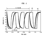
- FIG. 1 is a graph showing profiles of temperature cycles at two different frequencies.
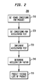
- FIG. 2 is a flowchart schematically illustrating a method for predicting a solder joint fatigue life according to an embodiment of the present invention.
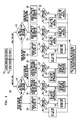
- FIG. 3 is a flowchart showing processing performed in Step 240 of the method shown in FIG. 2 .
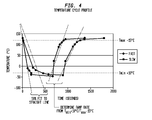
- FIG. 4 is a graph showing profiles of temperature cycles related to ramp rate.
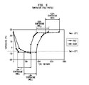
- FIG. 5 is a graph showing profiles of temperature cycles related to dwell time.
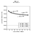
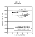
- FIG. 6 is a graph showing a function representing test fatigue life using a ramp rate.
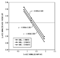
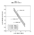
- FIG. 7 is a graph showing a linear function representing normalized test fatigue life using a normalized ramp rate.
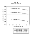
- FIG. 8 is a graph showing a function representing test fatigue life using a dwell time.
- FIG. 9 is a graph showing a linear function representing normalized test fatigue life using a normalized dwell time.
- the acceleration factor AF is a function of the temperature cycle frequency F. Because of the relationship to the temperature cycle frequency F lab for a laboratory environment in the denominator, m is 1 ⁇ 3 and a positive value. Thus, the value for the acceleration factor AF is smaller at a faster temperature cycle with a greater F lab value, and the value for the acceleration factor AF is larger at a slower temperature cycle with a smaller F lab value relative to a longer fatigue life. Therefore, the fatigue life is shorter.
- the oven conditions were JEDEC JESD 22-A104 Condition G ( ⁇ 45/125° C.) as shown in FIG. 1 .
- the T min minimum temperature
- the T max maximum temperature
- SoakMode2 was used.
- the temperature cycle frequencies are 2 cycles per hour (see 110 in FIG. 1 ) and 2.6 cycles per hour (see 120 in FIG. 1 ), with the holding time at T min and T max being a minimum of five minutes.
- the fatigue life was 20% faster, that is, shorter, at 2.6 cycles per hour, which is the slower temperature cycle frequency.
- the acceleration factor modeled and calculated in the finite element analysis is in harmony with actual experimental results, but a model has to be created in the finite element analysis simulation for each product shape to be tested.
- the results depend entirely on the equation representing the model, how the model is created, the boundary conditions, and the incorporated parameters. In other words, it is not generalized, and a simple fatigue life prediction method cannot be obtained.
- a solder joint fatigue life prediction method using the crack growth rate of the solder joint is also not a simple fatigue life prediction method because the crack growth rates have to be determined and used individually.
- the present invention realizes a simple method that is able to predict the fatigue life of a solder joint in a product.
- FIG. 2 is a flowchart schematically illustrating a method 200 for predicting a solder joint fatigue life according to an embodiment of the present invention.
- the field conditions of the solder-joined product include the maximum temperature T max — field , the minimum temperature T min — field , and the temperature cycle frequency F field under the field conditions of the product. These can be established by simply using the specifications of the product when available. At a minimum, the following items are usually provided in the specifications of a product.
- Step 220 the conditions for the accelerated testing are established.
- the conditions for the accelerated testing include the maximum temperature T max — lab , the minimum temperature T min — lab , and the temperature cycle frequency F lab in the laboratory environment for accelerated testing of the product.
- the accelerated testing can be performed under the JEDEC JESD 22-A104 Condition G ( ⁇ 45/125° C.) as shown in FIG. 1 .
- the T min (minimum temperature) is ⁇ 45° C.
- the T max (maximum temperature) is 125° C.
- SoakMode2 is used.
- the temperature cycle frequencies are 2 cycles per hour (see 110 in FIG. 1 ) and 2.6 cycles per hour (see 120 in FIG.
- the dwell time (holding time) at T min and T max being a minimum of five minutes.
- the maximum temperature T max — lab is established at 125° C.
- the minimum temperature T min — lab is established at ⁇ 45° C.
- the temperature cycle frequencies F lab are established at 2 cycles per hour and 2.6 cycles per hour.
- the accelerated testing is implemented under the established conditions (Step 230 ).
- the accelerated testing is implemented, and the test fatigue life N lab is measured until failure of the product. If the test fatigue life N lab can be measured in the accelerated testing by accelerating the failure of the product using the temperature load of the temperature cycle, an actual experiment does not have to be conducted. An experiment simulation able to faithfully reproduce an experiment can be employed.
- the acceleration factor is determined using a novel acceleration factor equation (Step 240 ).
- the novel acceleration factor equation can be either Equation 2 or Equation 3.
- An acceleration factor can be determined using either Equation 2 or Equation 3.
- Equation ⁇ ⁇ 2 AF ( ⁇ ⁇ ⁇ T field ⁇ ⁇ ⁇ T lab ) - n ⁇ ( Ramp field Ramp lab ) m 1 ⁇ ( Dwell field Dwell lab ) m 2 ⁇ ⁇ ⁇ E a R ⁇ ( 1 T max_field - 1 T max_lab ) ( Equation ⁇ ⁇ 2 )
- exponent m 1 for the ramp rate term [Ramp field /Ramp lab ] m1 and exponent m 2 for the dwell time term [Dwell field /Dwell lab ] m2 which are represented using the ramp rate Ramp field and the dwell time Dwell field of the field environment, and the ramp rate Ramp lab and the dwell time Dwell lab of the laboratory environment, are determined from the profile data of the temperature cycle using the established maximum temperature T max — field , the minimum temperature T min — field , and the temperature cycle frequency F field of the field environment established in Step 210 , from the profile data of the temperature cycle using the established maximum temperature T max — lab , of minimum temperature T min — lab , and the temperature cycle frequency F lab of the laboratory environment established in Step 220 , and from the test fatigue life N lab measured in Step 230 , and the acceleration factor AF is calculated by plugging the determined exponents m 1 and m 2 into Equation 2.
- exponent m 1 for the ramp rate term [Ramp field /Ramp lab ] m1 , exponent m 2 for the dwell time term [Dwell field /Dwell lab ] m2 , and exponent m 3 for the minimum temperature term [T min — field /T min — lab ] m3 which are represented using the ramp rate Ramp field , the dwell time Dwell field , and the minimum temperature T min — field of the field environment, and the ramp rate Ramp lab , the dwell time Dwell lab , and the minimum temperature T min — lab of the laboratory environment, are determined from the profile data of the temperature cycle using the established maximum temperature T max — field , the minimum temperature T min — field , and the temperature cycle frequency F field of the field environment established in Step 210 , from the profile data of the temperature cycle using the established maximum temperature T max — lab , the minimum temperature T min — lab , and the temperature cycle frequency F lab of the laboratory environment established in Step 220 , and from the measured
- the fatigue life of the product is estimated (Step 250 ).
- the fatigue life of the solder joint estimated in this way does not depend on the temperature cycle frequency as in the Modified Coffin-Manson Equation, but is derived in a newly devised way from the ramp rate and the dwell time or from the ramp rate, the dwell time and the minimum temperature. As a result, the fatigue life is more accurately reflected in accelerated testing, and matches experimental results more closely than the Modified Coffin-Manson Equation.
- FIG. 3 is a flowchart showing processing 300 performed in Step 240 of the method 200 .
- the temperature cycle profiles which represent the relationship between temperature and time, include the temperature cycle profile for the field environment and the temperature cycle profile for the laboratory environment.
- the temperature cycle profile data for the field environment is obtained from the maximum temperature T max — field , minimum temperature T min — field , and the temperature cycle frequency F field
- the temperature cycle profile data for the laboratory environment is obtained from the maximum temperature T max — lab , minimum temperature T min — lab , and the temperature cycle frequency F lab .
- a temperature cycle profile for the field environment can be obtained from the data in the following way.
- the power ON time is calculated as 40,000/3,000 ⁇ 13.3 hours/cycle, and the time per cycle is 13.3 hours.
- T min — field and the maximum temperature T max — field for the field environment of the product are ⁇ 10° C.
- the dwell times Dwell_High field and Dwell_Low field and the ramp rates RampUp field and RampDown field for the field environment can be obtained whether the high-temperature and low-temperature dwell times and the rising temperature and falling temperature ramp rates are the same or different.
- a temperature cycle profile for the laboratory environment can be obtained from the data in the following way.
- a temperature cycle profile for the laboratory environment is represented in a graph using temperature and time data.
- the graphs in FIG. 4 and FIG. 5 represent the relationship between temperature and time by linking the temperature (° C.) and the time (seconds) when the temperature cycle frequency is 2.6 cycles/hour (FAST) and when the temperature cycle frequency is 2 cycles/hour (SLOW).
- a single temperature cycle is shown in FIG. 4 and FIG. 5 , but a single cycle is enough to determine the temperature cycle profile because the same cycle is repeated.
- FIG. 4 and FIG. 5 show examples of temperature cycle profile data for two different temperature cycles, but the temperature cycle profile data can also be determined using a single temperature cycle frequency. When determined using a single temperature cycle frequency, various temperature cycle profiles can be obtained by varying the ramp rate and dwell time.
- the ramp rates for the laboratory environment include the rising temperature and falling temperature ramp rates RampUp lab and RampDown lab in the temperature cycle.
- the ramp rates for the laboratory environment can be determined from the temperature rate (unit: ° C./hour) for the portion of the relationship of the temperature and the time when the temperature is rising or falling which is a 90% fit with a straight line, or from the temperature rate (unit: ° C./hour) for a rising or falling temperature between the maximum temperature T max —lab ⁇ 15° C.
- the falling temperature ramp rate RampDown lab is determined from the temperature rate (unit: ° C./hour) for the portion which is a 90% fit with a straight line
- the rising temperature ramp rate RampUp lab is determined from the temperature rate (unit: ° C./hour) between the maximum temperature T max — lab ⁇ 15° C. and the minimum temperature T min — lab +10° C.
- the dwell times for the laboratory environment include high-temperature and low-temperature dwell times Dwell_High lab and Dwell_Low lab .
- the high-temperature dwell time Dwell_High lab can be the time the temperature is held between the maximum temperature T max — lab and the maximum temperature T max — lab ⁇ 15° C.
- the low-temperature dwell time Dwell_Low lab can be the time the temperature is held between the minimum temperature T min — lab and the minimum temperature T max — lab +10° C.
- the high-temperature dwell time Dwell_High lab is the time the product is held at a temperature between 110° C. (125-15° C.) and 125° C.
- the low-temperature dwell time Dwell_Low lab is the time the product is held at a temperature between ⁇ 35° C. ( ⁇ 45+10° C.) and ⁇ 45° C.
- the high-temperature and low-temperature dwell times Dwell_High lab and Dwell_Low lab are determined from the temperature cycle profiles.
- Step 320 it is first determined whether the sizes of the rising temperature and falling temperature ramp rates RampUp lab and RampDown lab are the same or different. In this determination, it is determined whether the sizes of these ramp rates RampUp lab and RampDown lab are different by 20% or more. If not, they are deemed to be the same. The faster or larger ramp rate is used as the reference, and it is determined by comparing 20% of the size to the difference between the sizes of both ramp rates.
- the process advances to Step 330 , and the correlation between the ramp rate and the fatigue life is calculated.
- the temperature cycle profile data is used to derive a function representing the test fatigue life N lab using at least three different ramp rates for at least three different dwell times.
- the three different dwell times may be the same at the high-temperature end, the low-temperature end, or both ends, and may be 5 minutes, 10 minutes and 20 minutes.
- the three different ramp rates at these dwell times may be the same for a rising temperature, a falling temperature, or both.
- test fatigue life N(50) at which 50% of the products in the accelerated testing failed A fatigue life N(50) at which 50% of the products in the accelerated testing fail is used as the test fatigue life N lab so as to take into account the implementation time of the accelerated testing.
- the test fatigue life N lab is not limited to fatigue life N(50). If the implementation time of the accelerated testing is not taken into account, any fatigue life N(P) at which 50% or more of the products in the accelerated testing fail can be used.
- 50 ⁇ P ⁇ 100 because 50% or more of the products have to fail in the accelerated testing in order to obtain a test fatigue life N lab that is reliable and accurate.
- the functions shown in FIG. 6 were derived by plotting the data in Table 1 on a graph in which the vertical axis denotes the fatigue life N(50) and the horizontal axis denotes the ramp rate. As shown in FIG. 6 , the fatigue life N(50) becomes smaller or shorter as the ramp rate becomes faster or larger.
- Step 332 the correlation with fatigue life is determined.
- Step 336 the process advances to Step 336 where the ramp rate term is calculated.
- the ramp rate term a linear function representing a normalized fatigue life N(50) using a normalized ramp rate is derived from a function representing the three fatigue lives N(50) derived in Step 330 (in the calculation of the correlation between the ramp rate and the fatigue life) using the ramp rate.
- the logarithms of the data in Table 1 are taken, and the values shown in Table 2 below are used.
- Step 340 the correlation between the ramp rate and the fatigue life during high-temperature rising is calculated.
- Step 350 the correlation between the ramp rate and the fatigue life during low-temperature falling is calculated.
- the data for the ramp rate is data for the ramp rate during high-temperature rising or data for the ramp rate during low-temperature falling. Data is obtained as shown in Table 1, and as shown in FIG. 6 , functions are derived representing the fatigue life N(50) using the ramp rate during high-temperature rising or the ramp rate during low-temperature falling.
- Step 342 and Step 352 the correlations with the fatigue life are determined. These determinations are performed in the same way as the determination in Step 332 . If the three functions derived in Step 340 or Step 350 are similar, the correlation with the fatigue life can be determined. If the three derived functions are different or the ramp rates do not change the fatigue life N(50) by more than 5% in the entire ramp rate range, it can be determined that there is no correlation between fatigue life and ramp rate.
- Step 342 When it has been determined in Step 342 that there is a correlation between the fatigue life and the high-temperature rising ramp rate, the process advances to Step 346 where the high-temperature rising ramp rate term is calculated.
- Step 352 When it has been determined in Step 352 that there is a correlation between the fatigue life and the low-temperature falling ramp rate, the process advances to Step 356 where the low-temperature falling ramp rate term is calculated.
- the calculation for the high-temperature rising ramp rate term and the calculation for the low-temperature falling ramp rate term are performed in the same way as the calculation in Step 336 .
- a linear function expressing a normalized fatigue life N(50) using a normalized high-temperature rising ramp rate is derived from a function representing the three fatigue lives N(50) derived in Step 340 (in the calculation of the correlation between the high-temperature rising ramp rate and the fatigue life) using the high-temperature rising ramp rate, determining, from the slope of the derived linear function, m 1a for [RampUp field /RampUp lab ] m1a , which is one portion of the ramp rate term [Ramp field /Ramp lab ] m1 , and [RampUp field /RampUp lab ] m1a is calculated.
- a value obtained in the manner described above is used for RampUp field , and a value obtained in accelerated testing is used for RampUp lab .
- a linear function expressing a normalized fatigue life N(50) using a normalized low-temperature falling ramp rate is derived from a function representing the three fatigue lives N(50) derived in Step 350 (in the calculation of the correlation between the low-temperature falling ramp rate and the fatigue life) using the low-temperature falling ramp rate, determining, from the slope of the derived linear function, m 1b for [RampDown field /RampDown lab ] m1b , which is one portion of the ramp rate term [Ramp field /Ramp lab ] m1 , and [RampDown field /RampDown lab ] m1b is calculated.
- Step 325 it is first determined whether the high-temperature and low-temperature dwell times are the same or different. In this determination, it is determined whether the dwell times Dwell_High lab and Dwell_Low lab are different by 20% or more. If not, they are deemed to be the same. The longer dwell time is used as the reference, and it is determined by comparing 20% of the longer time to the difference between both dwell times.
- the process advances to Step 360 , and the correlation between the dwell time and the fatigue life is calculated.
- the temperature cycle profile data is used to derive a function representing the test fatigue life N lab using at least three different dwell times for at least three different ramp rates.
- the three different ramp rates may be the same for a rising temperature, a falling temperature, or both. These may be 82.5° C./minute, 16.5° C./minute and 6.6° C./minute during a rising temperature.
- the three different dwell times at these ramp rates may be the same at the high-temperature end, the low-temperature end, or both ends, and may be 5 minutes, 10 minutes and 20 minutes.
- the results shown in Table 1 above were obtained when nine different combinations of these dwell times and ramp rates were applied to fatigue life N(50) at which 50% of the products in the accelerated testing failed.
- the functions shown in FIG. 8 are derived when the data in Table 1 is graphed with the vertical axis denoting the fatigue life N(50) and the horizontal axis denoting the dwell time.
- Step 362 the correlation with fatigue life is determined.
- Step 366 the dwell time term is calculated.
- a linear function representing a normalized fatigue life N(50) using a normalized dwell time is derived from a function representing the three fatigue lives N(50) derived in Step 360 (in the calculation of the correlation between the dwell time and the fatigue life) using the dwell time.
- the logarithms of the data in Table 1 are taken, and the values shown in Table 2 below are used.
- Step 370 the correlation between the high-temperature dwell time and the fatigue life is calculated.
- Step 380 the correlation between the low-temperature dwell time and the fatigue life is calculated.
- the data for the dwell time is data for the high-temperature dwell time or data for the low-temperature dwell time. Data is obtained as shown in Table 1, and as shown in FIG. 8 , functions are derived representing the fatigue life N(50) using the high-temperature dwell time or the low-temperature dwell time.
- Step 372 and Step 382 the correlations with the fatigue life are determined. These determinations are performed in the same way as the determination in Step 362 . If the three functions derived in Step 370 or Step 380 are similar, the correlation with the fatigue life can be determined. If the three derived functions are different or the dwell times do not change the fatigue life N(50) by more than 5% in the entire dwell time range, it can be determined that there is no correlation between fatigue life and dwell time.
- Step 372 When it has been determined in Step 372 that there is a correlation between the fatigue life and the high-temperature dwell time, the process advances to Step 376 where the high-temperature dwell time term is calculated.
- Step 382 When it has been determined in Step 382 that there is a correlation between the fatigue life and the low-temperature dwell time, the process advances to Step 386 where the low-temperature dwell time term is calculated.
- the calculation for the high-temperature dwell time term and the calculation for the low-temperature dwell time term are performed in the same way as the calculation in Step 366 .
- a linear function expressing a normalized fatigue life N(50) using a normalized high-temperature dwell time is derived from a function representing the three fatigue lives N(50) derived in Step 370 (in the calculation of the correlation between the high-temperature dwell time and the fatigue life) using the high-temperature dwell time, determining, from the slope of the derived linear function, m 2 a for [Dwell_High field /Dwell_High lab ] m2a , which is one portion of the dwell time term [Dwell field /Dwell lab ] m2 , and [Dwell_High field /Dwell_High lab ] m2a is calculated.
- a value obtained in the manner described above is used for Dwell_High field , and a value obtained in accelerated testing is used for Dwell_High lab .
- a linear function expressing a normalized fatigue life N(50) using a normalized low-temperature dwell time is derived from a function representing the three fatigue lives N(50) derived in Step 380 (in the calculation of the correlation between the low-temperature dwell time and the fatigue life) using the low-temperature dwell time, determining, from the slope of the derived linear function, m 2 b for [Dwell_Low field /Dwell_Low lab ] m2b , which is one portion of the dwell time term [Dwell field /Dwell lab ] m2 , and [Dwell_Low field /Dwell_Low lab ] m2b is calculated.
- Step 390 the values of the ramp rate term and the dwell time term corresponding to the calculations are plugged into the novel acceleration factor equation of Equation 2 or Equation 3, and the acceleration factor AF is calculated.
- the product of the acceleration factor AF calculated in process 300 of FIG. 3 and the fatigue life N(50) is determined to calculate the field fatigue life of the product, and the fatigue life of the product is predicted as shown in Step 250 of FIG. 2 .
- a minimum temperature term [T min — field /T min — lab ] m3 is included in the novel acceleration factor equation of Equation 3.
- the minimum temperature term is incorporated so as to take into account the effect of the minimum temperature on the fatigue life of a solder joint in the same manner as the ramp rate and dwell time.
- the value for the minimum temperature can be determined in the same way the values for the ramp rate term and the dwell time term were determined in FIG. 3 .
Landscapes
- Engineering & Computer Science (AREA)
- Physics & Mathematics (AREA)
- Computer Hardware Design (AREA)
- General Engineering & Computer Science (AREA)
- General Physics & Mathematics (AREA)
- Microelectronics & Electronic Packaging (AREA)
- Theoretical Computer Science (AREA)
- Evolutionary Computation (AREA)
- Geometry (AREA)
- Testing Of Devices, Machine Parts, Or Other Structures Thereof (AREA)
Abstract
A solder joint fatigue life predicting method includes: establishing a maximum temperature, a minimum temperature, and a temperature cycle frequency in a field environment; establishing a maximum temperature, a minimum temperature, and a temperature cycle frequency in a laboratory environment for accelerated testing; implementing the accelerated testing to measure test fatigue life until failure of the product; determining exponents for the ramp rate and dwell time in a novel acceleration factor equation which is represented using the ramp rates and dwell times of the field environment and the laboratory environment from profile data of the temperature cycle in the field environment, from profile data of the temperature cycle in the laboratory environment, and from test fatigue life data, and calculating an acceleration factor by plugging these exponents into the acceleration factor equation; and calculating field fatigue life of the product from the calculated acceleration factor and measured test fatigue life.
Description
- 1. Technical Field
- The present invention relates to predicting the fatigue life of a solder joint, and more specifically to a method for predicting the fatigue life of a solder joint using accelerated testing.
- 2. Background Art
- The Modified Coffin-Manson (Norris-Landzberg) Equation is the most commonly used method for predicting electrical component solder joint fatigue life. This equation is expressed as follows.
-
- In
Equation 1, the acceleration factor (AF) is a number representing the degree to which results from accelerated testing are accelerated relative to the field environment. The index “field” represents the field environment on the market, and “lab” represents the laboratory environment. ΔTfield and ΔTlab are the difference between the Tmax (maximum temperature) and the Tmin (minimum temperature) in a temperature cycle test repeating high and low temperatures. F is the frequency of the temperature cycle (representing the number of rising temperature and falling temperature cycles within a given period of time), Ffield is the temperature cycle frequency in the field environment, and Flab is the temperature cycle frequency in the laboratory environment. Tmax— field is the maximum temperature in the field environment, and Tmax— lab is the maximum temperature in the laboratory environment. Ea is the activation energy, and R is the Boltzmann Constant. - The activation energy Ea is a value (constant) determined from experimental results. The value used for 5Sn-95Pb solder is usually 0.123 eV in fatigue life estimates. The Boltzmann Constant R is 8.6159×10⁻⁵ eV/k (physical constant). The exponent n for ΔT (ΔTfield and ΔTlab) is a value (constant) determined from experimental results, with n=1.9 used for 5Sn-95Pb solder, and n=2.1 used for Pb-free solder. The exponent m for F (Ffield and Flab) is a value (constant) determined using Norris-Landsberg testing, where m=⅓. In accelerated testing, the ΔT, F and Tmax for the field environment (field) and the laboratory environment (lab) are known, and can be used in the calculation along with the constants to predict the fatigue life in the field environment (field) from experimental results. For example, when the test fatigue life of an experimental solder joint is 3,000 cycles, and the acceleration factor AF derived from the Modified Coffin-Manson Equation is 4.5, the following fatigue life is estimated for the field environment of the market: 3,000 cycles×4.5 (acceleration factor)=13,500 cycles.
- The fatigue life of the solder is predicted using finite element analysis, and the strain energy density is used as one of the parameters in predicting the fatigue life of the solder. The acceleration factor modeled and calculated in the finite element analysis is in harmony with actual experimental results.
- Also, methods for predicting the fatigue life of a solder joint have been proposed in which the crack growth rate of the solder joint is determined and used. These fatigue life prediction methods have been disclosed in the following patent literature:
- An aspect of the present invention is a method for predicting the fatigue life of a solder joint in a product joined by soldering, the method including the steps of: establishing a maximum temperature Tmax
— field, a minimum temperature Tmin— field, and a temperature cycle frequency Ffield in a field environment of the product; establishing a maximum temperature Tmax— lab, a minimum temperature Tmin— lab, and a temperature cycle frequency Flab in a laboratory environment for accelerated testing of the product; implementing the accelerated testing of the product to measure a test fatigue life Nlab until failure of the product; determining exponent m1 for the ramp rate and exponent m2 for the dwell time inEquation 2 below, which is represented using the ramp rate Ramp field and the dwell time Dwellfield of the field environment, and the ramp rate Ramp lab and the dwell time Dwelllab of the laboratory environment from the profile data of a temperature cycle using the established maximum temperature Tmax— field, the minimum temperature Tmin— field, and the temperature cycle frequency Ffield of the field environment, from the profile data of a temperature cycle using the established maximum temperature Tmax— lab, the minimum temperature Tmin— lab, and the temperature cycle frequency Flab of the laboratory environment, and from the measured data of the test fatigue life Nlab, and calculating an acceleration factor AF by plugging the determined exponents m1 and m2 intoEquation 2; and calculating a field fatigue life Nfield of the product from the calculated acceleration factor AF and the test fatigue life Nlab (Nfield=AF×Nlab). -
ΔT field =T max— field −T min— field -
ΔT lab =T max— lab −T min— lab - As understood by those skilled in the art, “ramp rate” is the rate at which the temperature rises to a high temperature or falls to a low temperature (unit: ° C./hour), and “dwell time” is the retention time at a predetermined high temperature or low temperature (unit: hours).
- In an embodiment, the step for calculating the acceleration factor AF further includes, when determining the exponent m1 for the term of the ramp rates Rampfield and Ramplab, determining whether or not the size of the ramp rate RampUplab and the ramp rate RampDownlab for a rising temperature and a falling temperature in the temperature cycle of the laboratory environment for the ramp rate Ramplab are the same or different.
- In an embodiment, when it has been determined that the size of the ramp rate RampUplab and the ramp rate RampDownlab for a rising temperature and a falling temperature in the temperature cycle of the laboratory environment are the same, a function is derived representing the test fatigue life Nlab using a ramp rate Ramplab corresponding to a ramp rate RampUplab or RampDownlab for a rising or falling temperature, and a correlation is determined between the test fatigue life Nlab and the ramp rate Ramplab.
- In an embodiment, when it has been determined in the determination of a correlation between the test fatigue life Nlab and the ramp rate Ramplab that there is no correlation, m1=0, and the ramp rate term [Rampfield/Ramplab]m1=1.
- In an embodiment, when it has been determined in the determination of a correlation between the test fatigue life Nlab and the ramp rate Ramplab that there is a correlation, a linear function representing a normalized test fatigue life Nlab using a normalized ramp rate Ramplab is derived from the function representing the test fatigue life Nlab using the ramp rate Ramplab, m1 is determined from the slope of the linear function, and the ramp rate term [Rampfield/Ramplab]m1 is calculated.
- In an embodiment, when it has been determined that the size of the ramp rate RampUplab and the ramp rate RampDownlab for a rising temperature and a falling temperature in the temperature cycle of the laboratory environment are different, a function is derived representing the test fatigue life Nlab using the ramp rate RampUplab during a rising high temperature and the correlation is determined between the test fatigue life Nlab and the ramp rate RampUplab during a rising high temperature, and a function is derived representing the test fatigue life Nlab using the ramp rate RampDownlab during a falling low temperature and the correlation is determined between the test fatigue life Nlab and the ramp rate RampDownlab during a falling low temperature.
- In an embodiment, when it has been determined in the determination of a correlation between the test fatigue life Nlab and the ramp rate during a rising high temperature RampUplab that there is no correlation, m1a=0 and [RampUpfield/RampUplab]m1a=1 for [RampUpfield/RampUplab]m1a constituting a portion of the ramp rate term [Rampfield/Ramplab]m1.
- In an embodiment, when it has been determined in the determination of a correlation between the test fatigue life Nlab and the ramp rate during a rising high temperature RampUplab that there is a correlation, a linear function representing a normalized test fatigue life Nlab using a normalized ramp rate during a rising high temperature RampUplab is derived from a function representing the test fatigue life Nlab using the ramp rate during a rising high temperature RampUplab, m1a is determined for [RampUpfield/RampUplab]m1a constituting a portion of the ramp rate term [Rampfield/Ramplab]m1 from the slope of the linear function, and [RampUpfield/RampUplab]m1a is calculated.
- In an embodiment, when it has been determined in the determination of a correlation between the test fatigue life Nlab and the ramp rate during a falling low temperature RampDownlab that there is no correlation, m1b=0 and [RampDownfield/RampDownlab]m1b=1 for [RampDownfield/RampDownlab]m1b constituting another portion of the ramp rate term [Rampfield/Ramplab]m1.
- In an embodiment, when it has been determined in the determination of a correlation between the test fatigue life Nlab and the ramp rate during a falling low temperature RampDownlab that there is a correlation, a linear function representing a normalized test fatigue life Nlab using a normalized ramp rate during a falling low temperature RampDownlab is derived from a function representing the test fatigue life Nlab using the ramp rate during a falling low temperature RampDownlab, m1b is determined for [RampDownfield/RampDownlab]m1b constituting another portion of the ramp rate term [Rampfield/Ramplab]m1 from the slope of the linear function, and [RampDownfield/RampDownlab]m1b is calculated.
- In an embodiment, the step for calculating the acceleration factor AF further includes, when determining the exponent m2 for the term of the dwell times Dwellfield and Dwelllab, determining whether or not a dwell time Dwell_Highlab and a dwell time Dwell_Lowlab for a high temperature and a low temperature in the laboratory environment for the dwell time Dwelllab are the same or different.
- In an embodiment, when it has been determined that the dwell time Dwell_Highlab and the dwell time Dwell_Lowlab for a high temperature and a low temperature in the laboratory environment are the same, a function is derived representing the test fatigue life Nlab using a dwell time Dwelllab corresponding to the Dwell_Highlab or the Dwell_Lowlab for a high temperature or a low temperature, and a correlation is derived between the test fatigue life Nlab and the dwell time Dwelllab.
- In an embodiment, when it has been determined in the determination of a correlation between the test fatigue life Nlab and the dwell time Dwelllab that there is no correlation, m2=0 and the dwell time term [Dwellfield/Dwelllab]m2=1.
- In an embodiment, when it has been determined in the determination of a correlation between the test fatigue life Nlab and the dwell time Dwelllab that there is a correlation, a linear function representing a normalized test fatigue life Nlab using a normalized dwell rate Dwelllab is derived from the function representing the test fatigue life Nlab using the dwell time Dwelllab, m2 is determined from the slope of the linear function, and the dwell time term [Dwellfield/Dwelllab]m2 is calculated.
- In an embodiment, when it has been determined that the dwell times Dwell_Highlab and the Dwell_Lowlab for a high temperature and a low temperature in the laboratory environment are different, a function is derived representing the test fatigue life Nlab using the dwell time Dwell_Highlab for a high temperature and the correlation is determined between the test fatigue life Nlab and the dwell time Dwell_Highlab for a high temperature, and a function is derived representing the test fatigue life Nlab using the dwell time Dwell_Lowlab for a low temperature and a correlation is determined between the test fatigue life Nlab and the dwell time Dwell_Lowlab for a low temperature.
- In an embodiment, when it has been determined in the determination of a correlation between the test fatigue life Nlab and the dwell time at high temperature Dwell_Highlab that there is no correlation, m2a=0 and [Dwell_Highfield/Dwell_Highlab]m2a=1 for [Dwell_Highfield/Dwell_Highlab]m2a constituting a portion of the dwell time term [Dwellfield/Dwelllab]m2.
- In an embodiment, when it has been determined in the determination of a correlation between the test fatigue life Nlab and the dwell time at high temperature Dwell_Highlab that there is a correlation, a linear function representing a normalized test fatigue life Nlab using a normalized dwell time at a high temperature Dwell_Highlab is derived from the function representing the test fatigue life Nlab using the dwell time at a high temperature Dwell_Highlab, m2a is determined for [Dwell_Highfield/Dwell_Highlab]m2a constituting a portion of the dwell time term [Dwellfield/Dwelllab]m2 from the slope of the linear function, and [Dwell_Highfield/Dwell_Highlab]m2a is calculated.
- In an embodiment, when it has been determined in the determination of a correlation between the test fatigue life Nlab and the dwell time at low temperature Dwell_Lowlab that there is no correlation, m2b=0 and [Dwell_Lowfield/Dwell_Lowlab]m2b=1 for [Dwell_Lowfield/Dwell_Lowlab]m2b constituting a portion of the dwell time term [Dwellfield/Dwelllab]m2.
- In an embodiment, when it has been determined in the determination of a correlation between the test fatigue life Nlab and the dwell time at low temperature Dwell_Lowlab that there is a correlation, a linear function representing a normalized test fatigue life Nlab using a normalized dwell time at a low temperature Dwell_Lowlab is derived from the function representing the test fatigue life Nlab using the dwell time at a low temperature Dwell_Lowlab, m2b is determined for [Dwell_Lowfield/Dwell_Lowlab]m2b, constituting another portion of the dwell time term [Dwellfield/Dwelllab]m2b from the slope of the linear function, and [Dwell_Lowfield/Dwell_Lowlab]m2b is calculated.
- A further aspect of the present invention is a method for predicting the fatigue life of a solder joint in a product joined by soldering, the method comprising the steps of: establishing a maximum temperature Tmax
— field, a minimum temperature Tmin— field, and a temperature cycle frequency Ffield in a field environment of the product; establishing a maximum temperature Tmax— lab, a minimum temperature Tmin— lab, and a temperature cycle frequency Flab in a laboratory environment for accelerated testing of the product; implementing the accelerated testing of the product to measure a test fatigue life Nlab until failure of the product; determining exponent m1 for the ramp rate, exponent m2 for the dwell time, and exponent m2 for the minimum temperature in Equation 3 below, which is represented using the ramp rate Rampfield and the dwell time Dwellfield of the field environment, and the ramp rate Ramplab and the dwell time Dwelllab of the laboratory environment from the profile data of a temperature cycle using the established maximum temperature Tmax— field, the minimum temperature Tmin— field, and the temperature cycle frequency Ffield of the field environment, from the profile data of a temperature cycle using the established maximum temperature Tmax— lab, the minimum temperature Tmin— lab, and the temperature cycle frequency Flab of the laboratory environment, and from the measured data of the test fatigue life Nlab, and calculating an acceleration factor AF by plugging the determined exponents m1, m2 and m3 into Equation 3; and calculating a field fatigue life Nfield of the product from the calculated acceleration factor AF and the test fatigue life Nlab (Nfield=AF×Nlab). -
ΔT field =T max— field −T min— field -
ΔT lab =T max— lab −T min— lab -
-
FIG. 1 is a graph showing profiles of temperature cycles at two different frequencies. -
FIG. 2 is a flowchart schematically illustrating a method for predicting a solder joint fatigue life according to an embodiment of the present invention. -
FIG. 3 is a flowchart showing processing performed inStep 240 of the method shown inFIG. 2 . -
FIG. 4 is a graph showing profiles of temperature cycles related to ramp rate. -
FIG. 5 is a graph showing profiles of temperature cycles related to dwell time. -
FIG. 6 is a graph showing a function representing test fatigue life using a ramp rate. -
FIG. 7 is a graph showing a linear function representing normalized test fatigue life using a normalized ramp rate. -
FIG. 8 is a graph showing a function representing test fatigue life using a dwell time. -
FIG. 9 is a graph showing a linear function representing normalized test fatigue life using a normalized dwell time. - In the commonly used Modified Coffin-Manson Equation, the acceleration factor AF is a function of the temperature cycle frequency F. Because of the relationship to the temperature cycle frequency Flab for a laboratory environment in the denominator, m is ⅓ and a positive value. Thus, the value for the acceleration factor AF is smaller at a faster temperature cycle with a greater Flab value, and the value for the acceleration factor AF is larger at a slower temperature cycle with a smaller Flab value relative to a longer fatigue life. Therefore, the fatigue life is shorter.
- However, an experiment was conducted in which the oven conditions were JEDEC JESD 22-A104 Condition G (−45/125° C.) as shown in
FIG. 1 . In other words, the Tmin (minimum temperature) was −45° C., the Tmax (maximum temperature) was 125° C., and SoakMode2 was used. Under these conditions, the temperature cycle frequencies are 2 cycles per hour (see 110 inFIG. 1 ) and 2.6 cycles per hour (see 120 inFIG. 1 ), with the holding time at Tmin and Tmax being a minimum of five minutes. As a result, the fatigue life was 20% faster, that is, shorter, at 2.6 cycles per hour, which is the slower temperature cycle frequency. In the calculation performed using the Modified Coffin-Manson Equation, 2 cycles per hour, which is the faster temperature cycle frequency, had a larger acceleration factor AF than 2.6 cycles per hour, which is the slower temperature cycle frequency, and the fatigue life was 9% shorter. Thus, the experimental results demonstrated that the fatigue life prediction for the solder joint of the product using the Modified Coffin-Manson Equation was not accurate. - The acceleration factor modeled and calculated in the finite element analysis is in harmony with actual experimental results, but a model has to be created in the finite element analysis simulation for each product shape to be tested. The results depend entirely on the equation representing the model, how the model is created, the boundary conditions, and the incorporated parameters. In other words, it is not generalized, and a simple fatigue life prediction method cannot be obtained. A solder joint fatigue life prediction method using the crack growth rate of the solder joint is also not a simple fatigue life prediction method because the crack growth rates have to be determined and used individually.
- The present invention realizes a simple method that is able to predict the fatigue life of a solder joint in a product.
- The following is an explanation of the present invention with reference to a preferred embodiment of the present invention. However, the present embodiment does not limit the present invention in the scope of the claims. Also, all combinations of characteristics explained in the embodiment are not necessarily required in the technical solution of the present invention. The present invention can be embodied in many different ways, and the present invention should not be interpreted as being limited to the content of the embodiment described below. In the explanation of the embodiment of the present invention, identical configurational units and configurational elements are denoted using the same reference signs.
-
FIG. 2 is a flowchart schematically illustrating amethod 200 for predicting a solder joint fatigue life according to an embodiment of the present invention. First, the field conditions of the solder-joined product are established (Step 210). The field conditions of the product include the maximum temperature Tmax— field, the minimum temperature Tmin— field, and the temperature cycle frequency Ffield under the field conditions of the product. These can be established by simply using the specifications of the product when available. At a minimum, the following items are usually provided in the specifications of a product. -
- Number of Years Under Product Warranty
- Power ON Time (Power ON Time Guarantee)
- ON/OFF Cycle (Number of Product ON/OFF Cycles)
- Minimum/Maximum Operating Environment Temperatures (Installation Environment of the Product)
- Minimum/Maximum Product Temperatures
- Maximum Power of Product
- Air Flow Rate During Cooling
- Next, the conditions for the accelerated testing are established (Step 220).
- The conditions for the accelerated testing include the maximum temperature Tmax
— lab, the minimum temperature Tmin— lab, and the temperature cycle frequency Flab in the laboratory environment for accelerated testing of the product. For example, the accelerated testing can be performed under the JEDEC JESD 22-A104 Condition G (−45/125° C.) as shown inFIG. 1 . In other words, the Tmin (minimum temperature) is −45° C., the Tmax (maximum temperature) is 125° C., and SoakMode2 is used. Under these conditions, the temperature cycle frequencies are 2 cycles per hour (see 110 inFIG. 1 ) and 2.6 cycles per hour (see 120 inFIG. 1 ), with the dwell time (holding time) at Tmin and Tmax being a minimum of five minutes. Thus, the maximum temperature Tmax— lab is established at 125° C., the minimum temperature Tmin— lab is established at −45° C., and the temperature cycle frequencies Flab are established at 2 cycles per hour and 2.6 cycles per hour. - Next, the accelerated testing is implemented under the established conditions (Step 230). The accelerated testing is implemented, and the test fatigue life Nlab is measured until failure of the product. If the test fatigue life Nlab can be measured in the accelerated testing by accelerating the failure of the product using the temperature load of the temperature cycle, an actual experiment does not have to be conducted. An experiment simulation able to faithfully reproduce an experiment can be employed.
- Next, the acceleration factor is determined using a novel acceleration factor equation (Step 240). The novel acceleration factor equation can be either
Equation 2 or Equation 3. An acceleration factor can be determined using eitherEquation 2 or Equation 3. -
- As for
Equation 2, exponent m1 for the ramp rate term [Rampfield/Ramplab]m1 and exponent m2 for the dwell time term [Dwellfield/Dwelllab]m2, which are represented using the ramp rate Rampfield and the dwell time Dwellfield of the field environment, and the ramp rate Ramplab and the dwell time Dwelllab of the laboratory environment, are determined from the profile data of the temperature cycle using the established maximum temperature Tmax— field, the minimum temperature Tmin— field, and the temperature cycle frequency Ffield of the field environment established inStep 210, from the profile data of the temperature cycle using the established maximum temperature Tmax— lab, of minimum temperature Tmin— lab, and the temperature cycle frequency Flab of the laboratory environment established inStep 220, and from the test fatigue life Nlab measured inStep 230, and the acceleration factor AF is calculated by plugging the determined exponents m1 and m2 intoEquation 2. -
- As for Equation 3, exponent m1 for the ramp rate term [Rampfield/Ramplab]m1, exponent m2 for the dwell time term [Dwellfield/Dwelllab]m2, and exponent m3 for the minimum temperature term [Tmin
— field/Tmin— lab]m3, which are represented using the ramp rate Rampfield, the dwell time Dwellfield, and the minimum temperature Tmin— field of the field environment, and the ramp rate Ramplab, the dwell time Dwelllab, and the minimum temperature Tmin— lab of the laboratory environment, are determined from the profile data of the temperature cycle using the established maximum temperature Tmax— field, the minimum temperature Tmin— field, and the temperature cycle frequency Ffield of the field environment established inStep 210, from the profile data of the temperature cycle using the established maximum temperature Tmax— lab, the minimum temperature Tmin— lab, and the temperature cycle frequency Flab of the laboratory environment established inStep 220, and from the measured data of the test fatigue life Nlab established inStep 230, and an acceleration factor AF is calculated by plugging the determined exponents m1, m2 and m3 into Equation 3. - Next, the fatigue life of the product is estimated (Step 250). The fatigue life of the product is estimated by calculating the field fatigue life Nfield of the product from the acceleration factor AF calculated using
Equation 2 or Equation 3, and from the measured test fatigue life Nlab (Nfield=AF×Nlab) The fatigue life of the solder joint estimated in this way does not depend on the temperature cycle frequency as in the Modified Coffin-Manson Equation, but is derived in a newly devised way from the ramp rate and the dwell time or from the ramp rate, the dwell time and the minimum temperature. As a result, the fatigue life is more accurately reflected in accelerated testing, and matches experimental results more closely than the Modified Coffin-Manson Equation. -
FIG. 3 is aflowchart showing processing 300 performed inStep 240 of themethod 200. First, the temperature cycle profiles are acquired (Step 310). The temperature cycle profiles, which represent the relationship between temperature and time, include the temperature cycle profile for the field environment and the temperature cycle profile for the laboratory environment. The temperature cycle profile data for the field environment is obtained from the maximum temperature Tmax— field, minimum temperature Tmin— field, and the temperature cycle frequency Ffield, and the temperature cycle profile data for the laboratory environment is obtained from the maximum temperature Tmax— lab, minimum temperature Tmin— lab, and the temperature cycle frequency Flab. - A temperature cycle profile for the field environment can be obtained from the data in the following way. When there are 3,000 ON/OFF cycles over 40,000 hours, the power ON time is calculated as 40,000/3,000≈13.3 hours/cycle, and the time per cycle is 13.3 hours. When the rising temperature and falling temperature times are 30 minutes each and the retention time at the high temperature and the low temperature are the same based on the characteristics of the product and its application, the dwell time for the field environment is Dwell_Highfield=Dwell_Lowfield=Dwellfield, or Dwellfield=[(40000/3000)−(0.5*2)]/2≈6.17 hours. When the minimum temperature Tmin
— field and the maximum temperature Tmax— field for the field environment of the product are −10° C. and 105° C., and the sizes of the ramp rates RampUpfield and RampDownfield during rising and falling temperatures are the same, the ramp rate for the field environment is RampUpfield=RampDownfield=Rampfield, or Rampfield=[105−(−10)]/30≈3.83° C./minute. In this way, the dwell times Dwell_Highfield and Dwell_Lowfield and the ramp rates RampUpfield and RampDownfield for the field environment can be obtained whether the high-temperature and low-temperature dwell times and the rising temperature and falling temperature ramp rates are the same or different. - A temperature cycle profile for the laboratory environment can be obtained from the data in the following way. In
FIG. 4 andFIG. 5 , a temperature cycle profile for the laboratory environment is represented in a graph using temperature and time data. The graphs inFIG. 4 andFIG. 5 represent the relationship between temperature and time by linking the temperature (° C.) and the time (seconds) when the temperature cycle frequency is 2.6 cycles/hour (FAST) and when the temperature cycle frequency is 2 cycles/hour (SLOW). A single temperature cycle is shown inFIG. 4 andFIG. 5 , but a single cycle is enough to determine the temperature cycle profile because the same cycle is repeated.FIG. 4 andFIG. 5 show examples of temperature cycle profile data for two different temperature cycles, but the temperature cycle profile data can also be determined using a single temperature cycle frequency. When determined using a single temperature cycle frequency, various temperature cycle profiles can be obtained by varying the ramp rate and dwell time. - Next, the temperature cycle profile is divided (Step 315), and the ramp rate term and the dwell time term are processed. Because the ramp rates and dwell times for the field environment have already been explained, the ramp rates and dwell times for the laboratory environment will now be explained. The ramp rates for the laboratory environment include the rising temperature and falling temperature ramp rates RampUplab and RampDownlab in the temperature cycle. The ramp rates for the laboratory environment can be determined from the temperature rate (unit: ° C./hour) for the portion of the relationship of the temperature and the time when the temperature is rising or falling which is a 90% fit with a straight line, or from the temperature rate (unit: ° C./hour) for a rising or falling temperature between the maximum temperature Tmax
—lab −15° C. and the minimum temperature Tmin— lab+10° C. InFIG. 4 , the falling temperature ramp rate RampDownlab is determined from the temperature rate (unit: ° C./hour) for the portion which is a 90% fit with a straight line, and the rising temperature ramp rate RampUplab is determined from the temperature rate (unit: ° C./hour) between the maximum temperature Tmax— lab−15° C. and the minimum temperature Tmin— lab+10° C. - The dwell times for the laboratory environment include high-temperature and low-temperature dwell times Dwell_Highlab and Dwell_Lowlab. In dwell times for the laboratory environment, the high-temperature dwell time Dwell_Highlab can be the time the temperature is held between the maximum temperature Tmax
— lab and the maximum temperature Tmax— lab−15° C., and the low-temperature dwell time Dwell_Lowlab can be the time the temperature is held between the minimum temperature Tmin— lab and the minimum temperature Tmax— lab+10° C. For example, when the maximum temperature Tmax— lab is 125° C., the high-temperature dwell time Dwell_Highlab is the time the product is held at a temperature between 110° C. (125-15° C.) and 125° C. When the minimum temperature Tmin— lab is −45° C., the low-temperature dwell time Dwell_Lowlab is the time the product is held at a temperature between −35° C. (−45+10° C.) and −45° C. As shown inFIG. 5 , the high-temperature and low-temperature dwell times Dwell_Highlab and Dwell_Lowlab are determined from the temperature cycle profiles. - When the ramp rate term shown on the left in
FIG. 3 is processed, it is first determined whether the sizes of the rising temperature and falling temperature ramp rates RampUplab and RampDownlab are the same or different (Step 320). In this determination, it is determined whether the sizes of these ramp rates RampUplab and RampDownlab are different by 20% or more. If not, they are deemed to be the same. The faster or larger ramp rate is used as the reference, and it is determined by comparing 20% of the size to the difference between the sizes of both ramp rates. - Next, when it has been determined that the sizes of the rising temperature and falling temperature ramp rates RampUplab and RampDownlab are the same, the process advances to Step 330, and the correlation between the ramp rate and the fatigue life is calculated. In this calculation, the temperature cycle profile data is used to derive a function representing the test fatigue life Nlab using at least three different ramp rates for at least three different dwell times. For example, the three different dwell times may be the same at the high-temperature end, the low-temperature end, or both ends, and may be 5 minutes, 10 minutes and 20 minutes. The three different ramp rates at these dwell times may be the same for a rising temperature, a falling temperature, or both. These may be 82.5° C./minute, 16.5° C./minute and 6.6° C./minute during a rising temperature. The results shown in Table 1 below were obtained when nine different combinations of these dwell times and ramp rates were applied to fatigue life N(50) at which 50% of the products in the accelerated testing failed. A fatigue life N(50) at which 50% of the products in the accelerated testing fail is used as the test fatigue life Nlab so as to take into account the implementation time of the accelerated testing. However, the test fatigue life Nlab is not limited to fatigue life N(50). If the implementation time of the accelerated testing is not taken into account, any fatigue life N(P) at which 50% or more of the products in the accelerated testing fail can be used. Here, 50≦P≦100 because 50% or more of the products have to fail in the accelerated testing in order to obtain a test fatigue life Nlab that is reliable and accurate.
-
TABLE 1 N(50) Fatigue Life Dwell Time (Minutes) 5 10 20 Rising 82.5 2389 2345 2308 Ramp Rate 16.5 2722 2677 2637 (° C./min.) 6.6 2926 2880 2837 - The functions shown in
FIG. 6 were derived by plotting the data in Table 1 on a graph in which the vertical axis denotes the fatigue life N(50) and the horizontal axis denotes the ramp rate. As shown inFIG. 6 , the fatigue life N(50) becomes smaller or shorter as the ramp rate becomes faster or larger. - Next, the correlation with fatigue life is determined (Step 332). In this determination, the derived functions are used. As shown in
FIG. 6 , the three derived functions are similar, and indicate the correlation between fatigue life and ramp rate. If the three derived functions are different or the ramp rates do not change the fatigue life N(50) by more than 5% in the entire ramp rate range, it can be determined that there is no correlation between fatigue life and ramp rate. In this situation, the process advances to Step 334, where m1=0 for the ramp rate term [Rampfield/Ramplab]m1 inEquation 2 or Equation 3, and [Rampfield/Ramplab]m1=1. Afterwards, the process advances to Step 390, and [Rampfield/Ramplab]m1=1 is used in the novel acceleration function equation ofEquation 2 or Equation 3. - When it has been determined in
Step 332 that there is a correlation between the fatigue life and the ramp rate, the process advances to Step 336 where the ramp rate term is calculated. In the calculation of the ramp rate term, a linear function representing a normalized fatigue life N(50) using a normalized ramp rate is derived from a function representing the three fatigue lives N(50) derived in Step 330 (in the calculation of the correlation between the ramp rate and the fatigue life) using the ramp rate. In this derivation, the logarithms of the data in Table 1 are taken, and the values shown in Table 2 below are used. -
TABLE 2 Normalized N(50) Fatigue Life Dwell Time 0.69897 1 1.30103 Rising 1.916454 3.378245 3.370086 3.363315 Ramp 1.217484 3.434904 3.427662 3.421146 Rate 0.819544 3.466319 3.45943 3.452926 - When numerical values in Table 2 are graphed with the vertical axis denoting the normalized fatigue life N(50) and the horizontal axis denoting the normalized ramp rate, the linear functions shown in
FIG. 7 are derived. The resulting slopes of the three linear functions are a coefficient of variable x. The average of the three slopes is taken as the slope of the linear function. Because the ramp rate is RampUplab=RampDownlab=Ramplab, m1 is obtained from the resulting slope, and the ramp rate term [Rampfield/Ramplab]m1 is calculated. A value obtained in the manner described above is used as Rampfield, and a value obtained in the accelerated testing is used as Ramplab. Afterwards, the process advances to Step 390, and the calculated ramp rate term [Rampfield/Ramplab]m1 is plugged into the novel acceleration factor equation inEquation 2 or Equation 3. - When it has been determined in
Step 320 that the sizes of the rising temperature and falling temperature ramp rates are different, the process advances to Step 340 orStep 350. InStep 340, the correlation between the ramp rate and the fatigue life during high-temperature rising is calculated. InStep 350, the correlation between the ramp rate and the fatigue life during low-temperature falling is calculated. These calculations are performed in the same way as the calculations inStep 330. However, the data for the ramp rate is data for the ramp rate during high-temperature rising or data for the ramp rate during low-temperature falling. Data is obtained as shown in Table 1, and as shown inFIG. 6 , functions are derived representing the fatigue life N(50) using the ramp rate during high-temperature rising or the ramp rate during low-temperature falling. - Next, the correlations with the fatigue life are determined (
Step 342 and Step 352). These determinations are performed in the same way as the determination inStep 332. If the three functions derived inStep 340 orStep 350 are similar, the correlation with the fatigue life can be determined. If the three derived functions are different or the ramp rates do not change the fatigue life N(50) by more than 5% in the entire ramp rate range, it can be determined that there is no correlation between fatigue life and ramp rate. In this situation, the process advances to Step 344 andStep 354, where m1a=0 for [RampUpfield/RampUplab]m1a, which is a portion of ramp rate term [Rampfield/Ramplab]m1 inEquation 2 or Equation 3, and [RampUpfield/RampUplab]m1a=1. Alternatively, m1b=0 for [RampDownfield/RampDownlab]m1b, which is a portion of ramp rate term [Rampfield/Ramplab]m1 inEquation 2 or Equation 3, and [RampDownfield/RampDownlab]m1b=1. Afterwards, the process advances to Step 390, and [RampUpfield/RampUplab]m1a=1 or [RampDownfield/RampDownlab]m1b=1 is used in the novel acceleration function equation ofEquation 2 or Equation 3. - When it has been determined in
Step 342 that there is a correlation between the fatigue life and the high-temperature rising ramp rate, the process advances to Step 346 where the high-temperature rising ramp rate term is calculated. When it has been determined inStep 352 that there is a correlation between the fatigue life and the low-temperature falling ramp rate, the process advances to Step 356 where the low-temperature falling ramp rate term is calculated. The calculation for the high-temperature rising ramp rate term and the calculation for the low-temperature falling ramp rate term are performed in the same way as the calculation inStep 336. A linear function expressing a normalized fatigue life N(50) using a normalized high-temperature rising ramp rate is derived from a function representing the three fatigue lives N(50) derived in Step 340 (in the calculation of the correlation between the high-temperature rising ramp rate and the fatigue life) using the high-temperature rising ramp rate, determining, from the slope of the derived linear function, m1a for [RampUpfield/RampUplab]m1a, which is one portion of the ramp rate term [Rampfield/Ramplab]m1, and [RampUpfield/RampUplab]m1a is calculated. A value obtained in the manner described above is used for RampUpfield, and a value obtained in accelerated testing is used for RampUplab. A linear function expressing a normalized fatigue life N(50) using a normalized low-temperature falling ramp rate is derived from a function representing the three fatigue lives N(50) derived in Step 350 (in the calculation of the correlation between the low-temperature falling ramp rate and the fatigue life) using the low-temperature falling ramp rate, determining, from the slope of the derived linear function, m1b for [RampDownfield/RampDownlab]m1b, which is one portion of the ramp rate term [Rampfield/Ramplab]m1, and [RampDownfield/RampDownlab]m1b is calculated. A value obtained in the manner described above is used for RampDownfield, and a value obtained in accelerated testing is used for RampDownlab. Afterwards, the process advances to Step 390, and the calculated ramp rate term [RampUpfield/RampUplab]m1a or [RampDownfield/RampDownlab]m1b is applied to the novel acceleration factor equation ofEquation 2 or Equation 3. - When the dwell time term shown on the right in
FIG. 3 is processed, it is first determined whether the high-temperature and low-temperature dwell times are the same or different (Step 325). In this determination, it is determined whether the dwell times Dwell_Highlab and Dwell_Lowlab are different by 20% or more. If not, they are deemed to be the same. The longer dwell time is used as the reference, and it is determined by comparing 20% of the longer time to the difference between both dwell times. - Next, when it has been determined that the high-temperature and low-temperature dwell times Dwell_Highlab and Dwell_Lowlab are the same, the process advances to Step 360, and the correlation between the dwell time and the fatigue life is calculated. In this calculation, the temperature cycle profile data is used to derive a function representing the test fatigue life Nlab using at least three different dwell times for at least three different ramp rates. For example, the three different ramp rates may be the same for a rising temperature, a falling temperature, or both. These may be 82.5° C./minute, 16.5° C./minute and 6.6° C./minute during a rising temperature. The three different dwell times at these ramp rates may be the same at the high-temperature end, the low-temperature end, or both ends, and may be 5 minutes, 10 minutes and 20 minutes. The results shown in Table 1 above were obtained when nine different combinations of these dwell times and ramp rates were applied to fatigue life N(50) at which 50% of the products in the accelerated testing failed. The functions shown in
FIG. 8 are derived when the data in Table 1 is graphed with the vertical axis denoting the fatigue life N(50) and the horizontal axis denoting the dwell time. - Next, the correlation with fatigue life is determined (Step 362). In this determination, the derived functions are used. As shown in
FIG. 8 , the three derived functions are similar, and indicate the correlation between fatigue life and ramp rate. If the three derived functions are different or the dwell times do not change the fatigue life N(50) by more than 5% in the entire dwell time range, it can be determined that there is no correlation between fatigue life and dwell time. In this situation, the process advances to Step 364, where m2=0 for the dwell time term [Dwellfield/Dwelllab]m2 inEquation 2 or Equation 3, and [Dwellfield/Dwelllab]m2=1. Afterwards, the process advances to Step 390, and [Dwellfield-Dwelllab]m2=1 is used in the novel acceleration function equation ofEquation 2 or Equation 3. - When it has been determined in
Step 362 that there is a correlation between the fatigue life and the dwell time, the process advances to Step 366 where the dwell time term is calculated. In the calculation of the dwell time term, a linear function representing a normalized fatigue life N(50) using a normalized dwell time is derived from a function representing the three fatigue lives N(50) derived in Step 360 (in the calculation of the correlation between the dwell time and the fatigue life) using the dwell time. In this derivation, the logarithms of the data in Table 1 are taken, and the values shown in Table 2 below are used. When numerical values in Table 2 are graphed with the vertical axis denoting the normalized fatigue life N(50) and the horizontal axis denoting the normalized dwell time, the linear functions shown inFIG. 9 are derived. The resulting slopes of the three linear functions are a coefficient of variable x. The average of the three slopes is taken as the slope of the linear function. Because the dwell time is Dwell_Highlab=Dwell_Lowlab=Dwelllab, m2 is obtained from the resulting slope, and the dwell time term [Dwellfield/Dwelllab]m2 is calculated. A value obtained in the manner described above is used as Dwellfield, and a value obtained in the accelerated testing is used as Dwelllab. Afterwards, the process advances to Step 390, and the calculated dwell time term [Dwellfield/Dwelllab]m2 is plugged into the novel acceleration factor equation inEquation 2 or Equation 3. - When it has been determined in
Step 325 that the high-temperature and low-temperature dwell times are different, the process advances to Step 370 orStep 380. InStep 370, the correlation between the high-temperature dwell time and the fatigue life is calculated. InStep 380, the correlation between the low-temperature dwell time and the fatigue life is calculated. These calculations are performed in the same way as the calculations inStep 360. However, the data for the dwell time is data for the high-temperature dwell time or data for the low-temperature dwell time. Data is obtained as shown in Table 1, and as shown inFIG. 8 , functions are derived representing the fatigue life N(50) using the high-temperature dwell time or the low-temperature dwell time. - Next, the correlations with the fatigue life are determined (
Step 372 and Step 382). These determinations are performed in the same way as the determination inStep 362. If the three functions derived inStep 370 orStep 380 are similar, the correlation with the fatigue life can be determined. If the three derived functions are different or the dwell times do not change the fatigue life N(50) by more than 5% in the entire dwell time range, it can be determined that there is no correlation between fatigue life and dwell time. In this situation, the process advances to Step 374 andStep 384, where m2a=0 for [Dwell_Highfield/Dwell_Highlab]m2a, which is a portion of dwell time term [Dwell_Highfield/Dwell_Highlab]m2 inEquation 2 or Equation 3, and [Dwell_Highfield/Dwell_Highlab]m2a=1. Alternatively, m2b=0 for [Dwell_Lowfield/Dwell_Lowlab]m2b, which is a portion of dwell time term [Dwellfield/Dwelllab]m2 inEquation 2 or Equation 3, and [Dwell_Lowfield/Dwell_Lowlab]m2b=1. Afterwards, the process advances to Step 390, and [Dwell_Highfield/Dwell_Highlab]m2a=1 or [Dwell_Lowfiled/Dwell_Lowlab]m2b=1 is used in the novel acceleration function equation ofEquation 2 or Equation 3. - When it has been determined in
Step 372 that there is a correlation between the fatigue life and the high-temperature dwell time, the process advances to Step 376 where the high-temperature dwell time term is calculated. When it has been determined inStep 382 that there is a correlation between the fatigue life and the low-temperature dwell time, the process advances to Step 386 where the low-temperature dwell time term is calculated. The calculation for the high-temperature dwell time term and the calculation for the low-temperature dwell time term are performed in the same way as the calculation inStep 366. A linear function expressing a normalized fatigue life N(50) using a normalized high-temperature dwell time is derived from a function representing the three fatigue lives N(50) derived in Step 370 (in the calculation of the correlation between the high-temperature dwell time and the fatigue life) using the high-temperature dwell time, determining, from the slope of the derived linear function, m2a for [Dwell_Highfield/Dwell_Highlab]m2a, which is one portion of the dwell time term [Dwellfield/Dwelllab]m2, and [Dwell_Highfield/Dwell_Highlab]m2a is calculated. A value obtained in the manner described above is used for Dwell_Highfield, and a value obtained in accelerated testing is used for Dwell_Highlab. A linear function expressing a normalized fatigue life N(50) using a normalized low-temperature dwell time is derived from a function representing the three fatigue lives N(50) derived in Step 380 (in the calculation of the correlation between the low-temperature dwell time and the fatigue life) using the low-temperature dwell time, determining, from the slope of the derived linear function, m2b for [Dwell_Lowfield/Dwell_Lowlab]m2b, which is one portion of the dwell time term [Dwellfield/Dwelllab]m2, and [Dwell_Lowfield/Dwell_Lowlab]m2b is calculated. A value obtained in the manner described above is used for Dwell_Lowfield, and a value obtained in accelerated testing is used for Dwell_Lowlab. Afterwards, the process advances to Step 390, and the calculated dwell time term [Dwell_Highfield/Dwell_Highlab]m2a or [Dwell_Lowfield/Dwell_Lowlab]m2b is applied to the novel acceleration factor equation ofEquation 2 or Equation 3. - Afterwards, in
Step 390, the values of the ramp rate term and the dwell time term corresponding to the calculations are plugged into the novel acceleration factor equation ofEquation 2 or Equation 3, and the acceleration factor AF is calculated. The product of the acceleration factor AF calculated inprocess 300 ofFIG. 3 and the fatigue life N(50) is determined to calculate the field fatigue life of the product, and the fatigue life of the product is predicted as shown inStep 250 ofFIG. 2 . - A minimum temperature term [Tmin
— field/Tmin— lab]m3 is included in the novel acceleration factor equation of Equation 3. The minimum temperature term is incorporated so as to take into account the effect of the minimum temperature on the fatigue life of a solder joint in the same manner as the ramp rate and dwell time. The value for the minimum temperature can be determined in the same way the values for the ramp rate term and the dwell time term were determined inFIG. 3 . - The present invention was explained using an embodiment, but the technical scope of the present invention is not limited to the embodiment described above. Various changes and improvements can be added to the embodiment, and embodiments with these changes and improvements are included within the technical scope of the present invention.
Claims (20)
1. A method for predicting the fatigue life of a solder joint in a product joined by soldering, the method comprising the steps of:
establishing a maximum temperature Tmax — field, a minimum temperature Tmin — field, and a temperature cycle frequency Ffield in a field environment of the product;
establishing a maximum temperature Tmax — lab, a minimum temperature Tmin — lab, and a temperature cycle frequency Flab in a laboratory environment for accelerated testing of the product;
implementing the accelerated testing of the product to measure a test fatigue life Nlab until failure of the product;
determining exponent m1 for the ramp rate and exponent m2 for the dwell time in Equation 1 below, which is represented using the ramp rate Rampfield and the dwell time Dwellfield of the field environment, and the ramp rate Ramplab and the dwell time Dwelllab of the laboratory environment from profile data of a temperature cycle using the established maximum temperature Tmax — field, the minimum temperature Tmin — field, and the temperature cycle frequency Ffield of the field environment, from profile data of a temperature cycle using the established maximum temperature Tmax — lab, the minimum temperature Tmin — lab, and the temperature cycle frequency Flab of the laboratory environment, and from measured data of the test fatigue life Nlab, and calculating an acceleration factor AF by plugging determined exponents m1 and m2 into Equation 1;
ΔT field =T max— field −T min — field
ΔT lab =T max— lab −T min — lab
ΔT field =T max
ΔT lab =T max
n: Constant Determined By Solder
Ea: Activation Energy
R: Boltzmann Constant
and calculating a field fatigue life Nfield of the product from the calculated acceleration factor AF and the test fatigue life Nlab (Nfield=AF×Nlab).
2. The method of claim 1 , wherein the step for calculating the acceleration factor AF further comprises, when determining the exponent m1 for the term of the ramp rates Rampfield and Ramplab, determining whether or not the size of a ramp rate RampUplab and a ramp rate RampDownlab for a rising temperature and a falling temperature in the temperature cycle of the laboratory environment for the ramp rate Ramplab are the same or different.
3. The method of claim 2 , further comprising, when it has been determined that the size of the ramp rate RampUplab and the ramp rate RampDownlab for a rising temperature and a falling temperature in the temperature cycle of the laboratory environment are the same, deriving a function representing the test fatigue life Nlab using a ramp rate Ramplab corresponding to the ramp rate RampUplab or the ramp rate RampDownlab for a rising or falling temperature, and determining a correlation between the test fatigue life Nlab and the ramp rate Ramplab.
4. The method of claim 3 , wherein, when it has been determined in the determination of a correlation between the test fatigue life Nlab and the ramp rate Ramplab that there is no correlation, m1=0, and the ramp rate term [Rampfield/Ramplab]m1=1.
5. The method of claim 3 , wherein, when it has been determined in the determination of a correlation between the test fatigue life Nlab and the ramp rate Ramplab that there is a correlation, a linear function representing a normalized test fatigue life Nlab using a normalized ramp rate Ramplab is derived from the function representing the test fatigue life Nlab using the ramp rate Ramplab, m1 is determined from the slope of the linear function, and the ramp rate term [Rampfield/Ramplab]m1 is calculated.
6. The method of claim 2 , further comprising, when it has been determined that the size of the ramp rate RampUplab and the ramp rate RampDownlab for a rising temperature and a falling temperature in the temperature cycle of the laboratory environment are different, deriving a function representing the test fatigue life Nlab using the ramp rate RampUplab during a rising high temperature and determining a correlation between the test fatigue life Nlab and the ramp rate RampUplab during a rising high temperature, and deriving a function representing the test fatigue life Nlab using the ramp rate RampDownlab during a falling low temperature and determining a correlation between the test fatigue life Nlab and the ramp rate RampDownlab during a falling low temperature.
7. The method of claim 6 , wherein, when it has been determined in the determination of a correlation between the test fatigue life Nlab and the ramp rate during a rising high temperature RampUplab that there is no correlation, m1a=0 and [RampUpfield/RampUplab]m1a=1 for [RampUpfield/RampUplab]m1a constituting a portion of the ramp rate term [Rampfield/Ramplab]m1.
8. The method of claim 6 , wherein, when it has been determined in the determination of a correlation between the test fatigue life Nlab and the ramp rate during a rising high temperature RampUplab that there is a correlation, a linear function representing a normalized test fatigue life Nlab using a normalized ramp rate during a rising high temperature RampUplab is derived from the function representing the test fatigue life Nlab using the ramp rate during a rising high temperature RampUplab, m1a is determined for [RampUpfield/RampUplab]m1a constituting a portion of the ramp rate term [Rampfield/Ramplab]m1 from the slope of the linear function, and [RampUpfield/RampUplab]m1a is calculated.
9. The method of claim 6 , wherein, when it has been determined in the determination of a correlation between the test fatigue life Nlab and the ramp rate during a falling low temperature RampDownlab that there is no correlation, m1b=0 and [RampDownfield/RampDownlab]m1b=1 for [RampDownfield/RampDownlab]m1b constituting another portion of the ramp rate term [Rampfield/Ramplab]m1.
10. The method of claim 6 , wherein, when it has been determined in the determination of a correlation between the test fatigue life Nlab and the ramp rate during a falling low temperature RampDownlab that there is a correlation, a linear function representing a normalized test fatigue life Nlab using a normalized ramp rate during a falling low temperature RampDownlab is derived from the function representing the test fatigue life Nlab using the ramp rate during a falling low temperature RampDownlab, m1b is determined for [RampDownfield/RampDownlab]m1b constituting another portion of the ramp rate term [Rampfield/Ramplab]m1 from the slope of the linear function, and [RampDownfield/RampDownlab]m1b is calculated.
11. The method of claim 1 , wherein the step for calculating the acceleration factor AF further comprises, when determining the exponent m2 for the term of the dwell times Dwellfield and Dwelllab, determining whether or not a dwell time Dwell_Highlab and a dwell time Dwell_Lowlab for a high temperature and a low temperature in the laboratory environment for the dwell time Dwelllab are the same or different.
12. The method of claim 11 , further comprising, when it has been determined that the dwell time Dwell_Highlab and the dwell time Dwell_Lowlab for a high temperature and a low temperature in the laboratory environment are the same, deriving a function representing the test fatigue life Nlab using a dwell time Dwelllab corresponding to the dwell time Dwell_Highlab or the dwell Dwell_Lowlab for a high temperature or a low temperature, and determining a correlation between the test fatigue life Nlab and the dwell time Dwelllab.
13. The method of claim 12 , wherein, when it has been determined in the determination of a correlation between the test fatigue life Nlab and the dwell time Dwelllab that there is no correlation, m2=0 and the dwell time term [Dwellfield/Dwelllab]m2=1.
14. The method of claim 12 , wherein, when it has been determined in the determination of a correlation between the test fatigue life Nlab and the dwell time Dwelllab that there is a correlation, a linear function representing a normalized test fatigue life Nlab using a normalized dwell rate Dwelllab is derived from the function representing the test fatigue life Nlab using the dwell time Dwelllab, m2 is determined from the slope of the linear function, and the dwell time term [Dwellfield/Dwelllab]m2 is calculated.
15. The method of claim 11 , further comprising, when it has been determined that the dwell times Dwell_Highlab and the Dwell_Lowlab for a high temperature and a low temperature in the laboratory environment are different, deriving a function representing the test fatigue life Nlab using the dwell time Dwell_Highlab for a high temperature and determining a correlation between the test fatigue life Nlab and the dwell time Dwell_Highlab for a high temperature, and deriving a function representing the test fatigue life Nlab using the dwell time Dwell_Lowlab for a low temperature and determining a correlation between the test fatigue life Nlab and the dwell time Dwell_Lowlab for a low temperature.
16. The method of claim 15 , wherein, when it has been determined in the determination of a correlation between the test fatigue life Nlab and the dwell time at high temperature Dwell_Highlab that there is no correlation, m2a=0 and [Dwell_Highfield/Dwell_Highlab]m2a=1 for [Dwell_Highfield/Dwell_Highlab]m2a constituting a portion of the dwell time term [Dwellfield/Dwelllab]m2.
17. The method of claim 15 , wherein, when it has been determined in the determination of a correlation between the test fatigue life Nlab and the dwell time at high temperature Dwell_Highlab that there is a correlation, a linear function representing a normalized test fatigue life Nlab using a normalized dwell time at a high temperature Dwell_Highlab is derived from the function representing the test fatigue life Nlab using the dwell time at a high temperature Dwell_Highlab, m2a is determined for [Dwell_Highfield/Dwell_Highlab]m2a constituting a portion of the dwell time term [Dwellfield/Dwelllab]m2 from the slope of the linear function, and [Dwell_Highfield/Dwell_Highlab]m2a is calculated.
18. The method of claim 15 , wherein, when it has been determined in the determination of a correlation between the test fatigue life Nlab and the dwell time at low temperature Dwell_Lowlab that there is no correlation, m2b=0 and [Dwell_Lowfield/Dwell_Lowlab]m2b=1 for [Dwell_Lowfield/Dwell_Lowlab]m2b constituting a portion of the dwell time term [Dwellfield/Dwelllab]m2.
19. The method of claim 15 wherein, when it has been determined in the determination of a correlation between the test fatigue life Nlab and the dwell time at low temperature Dwell_Lowlab that there is a correlation, a linear function representing a normalized test fatigue life Nlab using a normalized dwell time at a low temperature Dwell_Lowlab is derived from the function representing the test fatigue life Nlab using the dwell time at a low temperature Dwell_Lowlab, m2b is determined for [Dwell_Lowfield/Dwell_Lowlab]m2b constituting another portion of the dwell time term [Dwell/Dwellfield/Dwelllab]m2 from the slope of the linear function, and [Dwell_Lowfield/Dwell_Lowlab]m2b is calculated.
20. A method for predicting the fatigue life of a solder joint in a product joined by soldering, the method comprising the steps of:
establishing a maximum temperature Tmax — field, a minimum temperature Tmin — field, and a temperature cycle frequency Ffield in a field environment of the product;
establishing a maximum temperature Tmax — lab, a minimum temperature Tmin — lab, and a temperature cycle frequency Flab in a laboratory environment for accelerated testing of the product;
implementing the accelerated testing of the product to measure a test fatigue life Nlab until failure of the product;
determining exponent m1 for the ramp rate, exponent m2 for the dwell time, and exponent m3 for the minimum temperature in Equation 2 below, which is represented using the ramp rate Rampfield and the dwell time Dwellfield of the field environment, and the ramp rate Ramp lab and the dwell time Dwelllab of the laboratory environment from profile data of a temperature cycle using the established maximum temperature Tmax — field, the minimum temperature Tmin — field, and the temperature cycle frequency Ffield of the field environment, from profile data of a temperature cycle using the established maximum temperature Tmax — lab, the minimum temperature Tmin — lab, and the temperature cycle frequency Flab of the laboratory environment, and from the measured data of the test fatigue life Nlab, and calculating an acceleration factor AF by plugging the determined exponents m1, m2 and m3 into Equation 2;
ΔT field =T max— field −T min — field
ΔT lab =T max— lab −T min — lab
ΔT field =T max
ΔT lab =T max
n: Constant Determined By Solder
Ea: Activation Energy
R: Boltzmann Constant
and calculating a field fatigue life Nfield of the product from the calculated acceleration factor AF and the test fatigue life Nlab (Nfield=AF×Nlab).
Applications Claiming Priority (2)
| Application Number | Priority Date | Filing Date | Title |
|---|---|---|---|
| JP2012093407 | 2012-04-16 | ||
| JPJP2012093407 | 2012-04-16 |
Publications (1)
| Publication Number | Publication Date |
|---|---|
| US20130275096A1 true US20130275096A1 (en) | 2013-10-17 |
Family
ID=49325864
Family Applications (1)
| Application Number | Title | Priority Date | Filing Date |
|---|---|---|---|
| US13/801,162 Abandoned US20130275096A1 (en) | 2012-04-16 | 2013-03-13 | Solder Joint Fatigue Life Prediction Method |
Country Status (1)
| Country | Link |
|---|---|
| US (1) | US20130275096A1 (en) |
Cited By (11)
| Publication number | Priority date | Publication date | Assignee | Title |
|---|---|---|---|---|
| CN106092879A (en) * | 2016-06-07 | 2016-11-09 | 西安向阳航天材料股份有限公司 | Explosion clad pipe bonding state detection method based on vibratory response information |
| CN106153324A (en) * | 2016-07-28 | 2016-11-23 | 西安冠泰检测技术有限公司 | A kind of inflation fatigue test loading device |
| CN106644781A (en) * | 2016-12-20 | 2017-05-10 | 哈尔滨工业大学 | Metal fatigue life prediction method based on test piece surface temperature evolutionary analysis |
| CN109632489A (en) * | 2019-01-16 | 2019-04-16 | 西南交通大学 | A kind of Metal Material Fatigue crack propagation model construction method based on monotonic tension parameter |
| CN110059964A (en) * | 2019-04-22 | 2019-07-26 | 西安电子科技大学 | A kind of lead joint welding transmission performance evaluation method towards interconnection point defect |
| CN110726923A (en) * | 2018-07-16 | 2020-01-24 | 郑州宇通客车股份有限公司 | Accelerated life test method for motor controller circuit board |
| CN111208364A (en) * | 2019-12-17 | 2020-05-29 | 中国人民解放军92942部队 | Comprehensive stress reliability accelerated test method based on multiple models |
| CN111380772A (en) * | 2019-04-30 | 2020-07-07 | 中国人民解放军63961部队 | Method for measuring storage life of rubber sealing element in long-term storage product |
| CN112019158A (en) * | 2019-05-28 | 2020-12-01 | 汉能移动能源控股集团有限公司 | Outdoor life evaluation method and device for photovoltaic module |
| US10887979B2 (en) * | 2018-01-10 | 2021-01-05 | Hamilton Sunstrand Corporation | Low cycle fatigue prevention |
| EP3914054A4 (en) * | 2019-01-18 | 2022-01-19 | Mitsubishi Electric Corporation | Life prediction means for solder joint, and life prediction method for solder joint |
Citations (2)
| Publication number | Priority date | Publication date | Assignee | Title |
|---|---|---|---|---|
| US20070208548A1 (en) * | 2006-03-03 | 2007-09-06 | Solido Design Automation Inc. | Modeling of systems using canonical form functions and symbolic regression |
| US20130067424A1 (en) * | 2011-09-09 | 2013-03-14 | Renesas Electronics Corporation | Life prediction method of electronic device and design method of electronic device using the method |
-
2013
- 2013-03-13 US US13/801,162 patent/US20130275096A1/en not_active Abandoned
Patent Citations (2)
| Publication number | Priority date | Publication date | Assignee | Title |
|---|---|---|---|---|
| US20070208548A1 (en) * | 2006-03-03 | 2007-09-06 | Solido Design Automation Inc. | Modeling of systems using canonical form functions and symbolic regression |
| US20130067424A1 (en) * | 2011-09-09 | 2013-03-14 | Renesas Electronics Corporation | Life prediction method of electronic device and design method of electronic device using the method |
Non-Patent Citations (13)
| Title |
|---|
| Arnold, J., Reliability Testing of Ni-Modified SnCu and SAC305 Accelerated Thermal Cycling, 2008, Resistor, 1(1), 1. * |
| Clauset, A., Power-Law Distribution In Emperical Data, arXiv:0706.1062v2 [physics.data-an] 2 Feb 2009 * |
| Clech, J., Closed-Form, Strain-Energy-Based Acceleration Factors for Thermal Cycling of Lead-Free Assemblies, Tuesday, February 2, 2010 teaches to build a AF model that includes dwell time. See below. * |
| Clech, J.P., Acceleration Factors and Thermal Cycling Test Efficincy for Lead-Free SN-AG-CU Assembliers, SMTAI 2005. * |
| ESPEC_2007.pdf, Yuichi Aoki, Ichisaku Tsujie, Takayuki Nagai, The effect of ramp rate on temperature cycle fatique in solder joints, ESPEC Technology Report No. 25 , September 15, 2007 * |
| ESPEC_2008.pdf, Yuichi Aoki, Ichisaku Tsujie, Takayuki Nagai, The effect of ramp rate on temperature cycle fatique in solder joints, ESPEC Technology Report No. 27, 2008 * |
| Falk, R., Many Faces of the Correlation Coefficient, Journal of Statistics Education v.5, N.3 (1997) * |
| Hopkins, W.G., A New View of Statistics: P Values, 2002, http://www.sportsci.org/resource/stats/pvalues.html * |
| Maydeu-Olivares, A., Goodness-of-Fit Testing, International Encyclopedia of Education (2010), vol. 7, pp. 190-196 * |
| Salmela, O., Acceleration Factors for Lead-Free Solder Materials, IEEE Transactions on Components and Packaging Technology, Vol., 30, No. 4, December 2007. * |
| Tasooji, A., Design Parameters Influencing Reliability of CCGA Assembly: A Sensitivity Analysis, IEEE 2006 * |
| Weglinski, R., Highly Accelerated Stress Screening for Air-cooled Switching Power Supplies, Part 1 Understanding Stress Test Methodology, White Papter: TW0058, February 1, 2007, TCI Power * |
| Zhai, C., Board Level Solder Reliability Versus Ramp Rate and Dwell time During Temperature Cycling, IEEE Transactions on Device and Materials Reliability, Vol. 3, No. 44, December 2003 * |
Cited By (12)
| Publication number | Priority date | Publication date | Assignee | Title |
|---|---|---|---|---|
| CN106092879A (en) * | 2016-06-07 | 2016-11-09 | 西安向阳航天材料股份有限公司 | Explosion clad pipe bonding state detection method based on vibratory response information |
| CN106153324A (en) * | 2016-07-28 | 2016-11-23 | 西安冠泰检测技术有限公司 | A kind of inflation fatigue test loading device |
| CN106644781A (en) * | 2016-12-20 | 2017-05-10 | 哈尔滨工业大学 | Metal fatigue life prediction method based on test piece surface temperature evolutionary analysis |
| US10887979B2 (en) * | 2018-01-10 | 2021-01-05 | Hamilton Sunstrand Corporation | Low cycle fatigue prevention |
| CN110726923A (en) * | 2018-07-16 | 2020-01-24 | 郑州宇通客车股份有限公司 | Accelerated life test method for motor controller circuit board |
| CN109632489A (en) * | 2019-01-16 | 2019-04-16 | 西南交通大学 | A kind of Metal Material Fatigue crack propagation model construction method based on monotonic tension parameter |
| EP3914054A4 (en) * | 2019-01-18 | 2022-01-19 | Mitsubishi Electric Corporation | Life prediction means for solder joint, and life prediction method for solder joint |
| US20220105583A1 (en) * | 2019-01-18 | 2022-04-07 | Mitsubishi Electric Corporation | Solder joint life predictor and solder joint life prediction method |
| CN110059964A (en) * | 2019-04-22 | 2019-07-26 | 西安电子科技大学 | A kind of lead joint welding transmission performance evaluation method towards interconnection point defect |
| CN111380772A (en) * | 2019-04-30 | 2020-07-07 | 中国人民解放军63961部队 | Method for measuring storage life of rubber sealing element in long-term storage product |
| CN112019158A (en) * | 2019-05-28 | 2020-12-01 | 汉能移动能源控股集团有限公司 | Outdoor life evaluation method and device for photovoltaic module |
| CN111208364A (en) * | 2019-12-17 | 2020-05-29 | 中国人民解放军92942部队 | Comprehensive stress reliability accelerated test method based on multiple models |
Similar Documents
| Publication | Publication Date | Title |
|---|---|---|
| US20130275096A1 (en) | Solder Joint Fatigue Life Prediction Method | |
| JP7266587B2 (en) | Method and system for controlling rechargeable batteries | |
| US20190138926A1 (en) | Degradation modeling and lifetime prediction method considering effective shocks | |
| CN104820781B (en) | Consider that temperature follows the BGA thermal fatigue life of solder joint Forecasting Methodologies of load sequence loading effect | |
| CN103246821B (en) | A kind of many stress small sample accelerated life test plan design optimization method based on emulation | |
| US9093844B2 (en) | Charge/discharge scheduling system and charge/discharge scheduling method | |
| US11719760B2 (en) | Probabilistic determination of transformer end of life | |
| US8965712B2 (en) | Life predicting method for solder joint, life predicting apparatus for solder joint and electronic device | |
| KR101526313B1 (en) | Method for predicting fatigue life | |
| US11841402B2 (en) | Battery state estimation device | |
| US10126373B2 (en) | Inspection method of secondary battery | |
| JP7202958B2 (en) | Storage battery condition evaluation system | |
| US20170167741A1 (en) | Air conditioning parameter generation apparatus, air conditioning operational evaluation apparatus, method and non-transitory computer readable medium | |
| JP5808285B2 (en) | Solder joint life prediction method | |
| CN111239515A (en) | Current-carrying fault prediction method and system for power equipment | |
| Lamár et al. | Average probability of failure of aperiodically operated devices | |
| US10605868B2 (en) | Performance tracking of an electrical energy storage system | |
| CN106991074A (en) | Accelerated degradation test Optimization Design based on accelerated factor principle of invariance | |
| US10935966B2 (en) | Product inspection device, product inspection method, and computer program | |
| Baussaron et al. | Degradation test plan for Wiener degradation processes | |
| US10733331B2 (en) | Information processing apparatus, information processing method, and recording medium | |
| KR101726483B1 (en) | Apparatus and method for battery usage pattern analysis | |
| CN112834942A (en) | Battery management system service life testing method and device based on temperature alternation test | |
| JP2013024671A (en) | Semiconductor integrated circuit test method, system, and program | |
| CN112986733B (en) | Storage reliability evaluation method of electronic product |
Legal Events
| Date | Code | Title | Description |
|---|---|---|---|
| AS | Assignment |
Owner name: INTERNATIONAL BUSINESS MACHINES CORPORATION, NEW Y Free format text: ASSIGNMENT OF ASSIGNORS INTEREST;ASSIGNORS:YOSHIMURA, AKIFUMI;OKAMOTO, KEISHI;REEL/FRAME:029988/0397 Effective date: 20130313 |
|
| STCB | Information on status: application discontinuation |
Free format text: ABANDONED -- FAILURE TO RESPOND TO AN OFFICE ACTION |