JP5448827B2 - Method and apparatus for generating a route - Google Patents
Method and apparatus for generating a route Download PDFInfo
- Publication number
- JP5448827B2 JP5448827B2 JP2009535133A JP2009535133A JP5448827B2 JP 5448827 B2 JP5448827 B2 JP 5448827B2 JP 2009535133 A JP2009535133 A JP 2009535133A JP 2009535133 A JP2009535133 A JP 2009535133A JP 5448827 B2 JP5448827 B2 JP 5448827B2
- Authority
- JP
- Japan
- Prior art keywords
- route
- destination
- source
- cost
- routing tree
- Prior art date
- Legal status (The legal status is an assumption and is not a legal conclusion. Google has not performed a legal analysis and makes no representation as to the accuracy of the status listed.)
- Expired - Fee Related
Links
Images


Classifications
-
- G—PHYSICS
- G09—EDUCATION; CRYPTOGRAPHY; DISPLAY; ADVERTISING; SEALS
- G09B—EDUCATIONAL OR DEMONSTRATION APPLIANCES; APPLIANCES FOR TEACHING, OR COMMUNICATING WITH, THE BLIND, DEAF OR MUTE; MODELS; PLANETARIA; GLOBES; MAPS; DIAGRAMS
- G09B29/00—Maps; Plans; Charts; Diagrams, e.g. route diagram
- G09B29/10—Map spot or coordinate position indicators; Map reading aids
- G09B29/106—Map spot or coordinate position indicators; Map reading aids using electronic means
-
- G—PHYSICS
- G01—MEASURING; TESTING
- G01C—MEASURING DISTANCES, LEVELS OR BEARINGS; SURVEYING; NAVIGATION; GYROSCOPIC INSTRUMENTS; PHOTOGRAMMETRY OR VIDEOGRAMMETRY
- G01C21/00—Navigation; Navigational instruments not provided for in groups G01C1/00 - G01C19/00
- G01C21/26—Navigation; Navigational instruments not provided for in groups G01C1/00 - G01C19/00 specially adapted for navigation in a road network
- G01C21/34—Route searching; Route guidance
- G01C21/3446—Details of route searching algorithms, e.g. Dijkstra, A*, arc-flags, using precalculated routes
-
- G—PHYSICS
- G06—COMPUTING; CALCULATING OR COUNTING
- G06Q—INFORMATION AND COMMUNICATION TECHNOLOGY [ICT] SPECIALLY ADAPTED FOR ADMINISTRATIVE, COMMERCIAL, FINANCIAL, MANAGERIAL OR SUPERVISORY PURPOSES; SYSTEMS OR METHODS SPECIALLY ADAPTED FOR ADMINISTRATIVE, COMMERCIAL, FINANCIAL, MANAGERIAL OR SUPERVISORY PURPOSES, NOT OTHERWISE PROVIDED FOR
- G06Q10/00—Administration; Management
- G06Q10/04—Forecasting or optimisation specially adapted for administrative or management purposes, e.g. linear programming or "cutting stock problem"
- G06Q10/047—Optimisation of routes or paths, e.g. travelling salesman problem
-
- G—PHYSICS
- G06—COMPUTING; CALCULATING OR COUNTING
- G06Q—INFORMATION AND COMMUNICATION TECHNOLOGY [ICT] SPECIALLY ADAPTED FOR ADMINISTRATIVE, COMMERCIAL, FINANCIAL, MANAGERIAL OR SUPERVISORY PURPOSES; SYSTEMS OR METHODS SPECIALLY ADAPTED FOR ADMINISTRATIVE, COMMERCIAL, FINANCIAL, MANAGERIAL OR SUPERVISORY PURPOSES, NOT OTHERWISE PROVIDED FOR
- G06Q30/00—Commerce
- G06Q30/02—Marketing; Price estimation or determination; Fundraising
- G06Q30/0283—Price estimation or determination
-
- H—ELECTRICITY
- H04—ELECTRIC COMMUNICATION TECHNIQUE
- H04L—TRANSMISSION OF DIGITAL INFORMATION, e.g. TELEGRAPHIC COMMUNICATION
- H04L45/00—Routing or path finding of packets in data switching networks
- H04L45/12—Shortest path evaluation
-
- H—ELECTRICITY
- H04—ELECTRIC COMMUNICATION TECHNIQUE
- H04L—TRANSMISSION OF DIGITAL INFORMATION, e.g. TELEGRAPHIC COMMUNICATION
- H04L45/00—Routing or path finding of packets in data switching networks
- H04L45/34—Source routing
Description
本発明は、加重有向グラフにおいて複数の多様なルートを生成する方法および装置に関する。 The present invention relates to a method and apparatus for generating a plurality of diverse routes in a weighted directed graph.
本明細書で用いられる用語「多様なルート(diverse routes)」とは、それらの長さの予め定められた比率よりも小さい比率で(通常はそれらの長さの85%未満の比率で)同じリンクを共有するルートを意味する。 As used herein, the term “diverse routes” is the same at a ratio that is less than a predetermined ratio of their lengths (typically less than 85% of their lengths). Means a route sharing a link.
グラフG=<V,E>は、頂点の集合(別名位置またはノード)Vおよびエッジの集合(別名アークまたはリンク)Eから成る。エッジは、2つの頂点uおよびvを接続する。vは、uに隣接していると言われている。有向グラフにおいては、各エッジは、uからvまで方向性を有し、順序対(ordered pair) <u,v>またはu->vとして書かれている。無向グラフにおいては、エッジは、方向性を有しなくて、非順序対(unordered pair){u、v}またはu<−>vとして書かれる。あらゆる無向エッジ{u、v}が2つの有向エッジ<u、v>および<v、u>により表される場合、無向グラフは有向グラフにより表されることができる。 The graph G = <V, E> consists of a set of vertices (also known as positions or nodes) V and a set of edges (also known as arcs or links) E. An edge connects two vertices u and v. v is said to be adjacent to u. In a directed graph, each edge is directional from u to v and is written as ordered pair <u, v> or u-> v. In undirected graphs, edges are not oriented and are written as unordered pairs {u, v} or u <-> v. An undirected graph can be represented by a directed graph if every undirected edge {u, v} is represented by two directed edges <u, v> and <v, u>.
有向および無向グラフには、重み付けをすることができる。重みは、各エッジに付与される。これは、例えば、2つの都市の間の距離、ドライブ時間、旅行の費用、電気径路(パス)の抵抗その他の、エッジと関連した量を表すために用いられることが可能である。特にグラフがある種のマップを表すとき、重みはエッジの長さまたはコストと呼ばれることがある。重みまたはパスまたはサイクルの長さは、重みまたはそのコンポーネント・エッジの長さの合計である。 Directed and undirected graphs can be weighted. A weight is assigned to each edge. This can be used, for example, to represent an edge-related quantity, such as distance between two cities, drive time, travel costs, electrical path resistance, etc. The weight may be referred to as edge length or cost, especially when the graph represents some kind of map. The weight or path or cycle length is the sum of the weight or length of its component edges.
この出願に記載されている方法は、通常、コストが加重有向グラフによって、記載でき、そのグラフに負のコストのサイクルがない如何なる領域にも適用可能である。我々は実施例の多くにおいて、ルーティングを道路網に用いている、しかし、この技術が他のドメイン、たとえば、交換点のネットワーク周辺でのパケットの中のルーティングや、集積回路、プリント回路基板または建物の配線のためのパスの発見等においても、等しくよく適用できることを理解すべきである。 The method described in this application is generally applicable to any region where the cost can be described by a weighted directed graph and the graph does not have a negative cost cycle. In many of the embodiments we use routing in the road network, but this technology is used for routing in packets around other domains, eg, switching point networks, integrated circuits, printed circuit boards or buildings. It should be understood that the present invention can be applied equally well in the discovery of the path for the other wiring.
道ルート・プランナは、ソースAから目的地Bまでの最適ルートを見つけるように設計されている。それらは、これを最小限のコストを有する単一のルートとして定義する。ここで、コスト関数は、時間、ジャンクション遅延、距離、財政的なコスト、ルートを形成するリンクの道のタイプの単純な加重和(総和)である。これらの方法は、「最短パス」としばしば呼ばれているが、これは、コスト(それらが何を表すにせよ)の合計において、最短であることを意味し、必ずしもメートルにおいて、最短であることを意味するものではないと理解される。所与のコスト関数および道グラフに対して、AからBへの最も低いコストが存在する。そして、これは周知のアルゴリズム、例えばダイクストラのアルゴリズムを用いることにより発見できる。退化ケースにおいては、グローバルに最低のコストを共有する複数のルートがある場合があるが、上記アルゴリズムはそれらのうちの1つだけを見つけ出す。ダイクストラのアルゴリズムは実際にAからすべてのノードまでの最適ルートを捜し出す。しかし、そのアルゴリズムのバリエーションは、早期に終了しBの方向を優先して調査するように設計されている。グラフへの主たる制約は、負の全体コストを有するサイクルがあってはならないことであり、それはすべてのコストが正である道路網について満足させるのに十分単純なものである。 The road route planner is designed to find the best route from source A to destination B. They define this as a single route with minimal cost. Here, the cost function is time, junction delay, distance, financial cost, and a simple weighted sum (sum) of the types of link paths that form the route. These methods are often referred to as “shortest paths”, which means they are the shortest in the sum of the costs (whatever they represent), and are necessarily shortest in meters Is understood not to mean. For a given cost function and road graph, there is the lowest cost from A to B. This can be found by using a well-known algorithm such as Dijkstra's algorithm. In the degenerate case, there may be multiple routes sharing the lowest cost globally, but the algorithm finds only one of them. Dijkstra's algorithm actually finds the optimal route from A to all nodes. However, the algorithm variations are designed to end early and to prioritize the direction of B. The main constraint to the graph is that there should be no cycle with a negative overall cost, which is simple enough to satisfy a road network where all costs are positive.
異なるルート・プランナは、わずかに異なる道データベースおよびコスト関数を有する。それらは、AからBまでの等しくもっともらしいルート(時々相互に非常に異なる)を見つけ出すことができる。すべてのこの種のもっともらしいルート(特に互いに非常に相違するルート)を見ることは、ユーザにとって便利である。 Different route planners have slightly different road databases and cost functions. They can find equally plausible routes from A to B (sometimes very different from each other). It is convenient for the user to see all such plausible routes, especially those that are very different from each other.
推奨されたルートがユーザが推測したか好んだものでないとわかることは一般にあることである。したがって、彼らは、時間および距離を比較できるように、ルート・プランナに彼らのルートを選ばせようとする。これは、道に沿って強制的なストップを加えることによって、または、ルーターが回避することになっている道リンク、ジャンクションまたは領域を指定することによって、または、コスト関数の加重を変えてより早い、より短い、より多くの高速道路ルートまたは他の基準の方を優先することによって、達成される。これは非常に時間がかかることがありえる。そして、しばしば、人は、他の人であれば試したであろうより良好なルートがあるのではないかと考えるままにされている。 It is common to see that the recommended route is not what the user guessed or liked. Therefore, they try to have the route planner choose their route so that they can compare time and distance. This is faster by adding a forced stop along the road, or by specifying a road link, junction or area that the router is supposed to avoid, or by changing the weight of the cost function Achieved by prioritizing shorter, more highway routes or other criteria. This can be very time consuming. And often people are left to think that there is a better route that others would have tried.
例えば、ケンブリッジからマンチェスターまで移動することを考える。1つのルート・ファインダーは、A14、それからM6、M56を用いることを提案する。別のものは、M6料金(M6 toll)を用いる。更に別のものは、A14それに続くA1を推奨する。これらの全ては、上手な人間のプランナが選ぶであろうルートの中にあるが、我々はそれ以外のものをどうやって見つけるのであろうか。 For example, consider moving from Cambridge to Manchester. One route finder proposes to use A14, then M6, M56. Another uses an M6 fee (M6 toll). Still another recommends A14 followed by A1. All of these are in the route that a good human planner would choose, but how do we find others?
大部分の単一の最短路ルーターの基礎は、ダイクストラのアルゴリズムの何らかのバリエーションである。このアルゴリズムについての良いオリジナル参考文献は、E.W. Dijkstra. 「A note on two problems in connexion with graphs グラフに関しての2つの問題についての覚書」Numerische Matematik 1:269-271(1959)である。 The basis of most single shortest path routers is some variation of Dijkstra's algorithm. A good original reference for this algorithm is E.W. Dijkstra. “A note on two problems in connexion with graphs” Memurische Matematik 1: 269-271 (1959).
これらのアルゴリズムは、ソースから任意のノードに着くためにそれまでに見つかった最も低いコストを維持する。それらは、(異なるヒューリスティック、例えばA*アルゴリズムに基づいて)低コストを有する活動ノード(出リンクがまだ調査されることを必要とするもの)を繰り返し選択し、幾つかの出エッジを探査して、それらがこれまでに記録されたものよりも低いコストの別のノードに達することができるかどうかを見る。 These algorithms maintain the lowest cost ever found to get to any node from the source. They repeatedly select active nodes (those that require the outgoing link still to be probed) and explore several outgoing edges (based on different heuristics, eg A * algorithm) See if they can reach another node with a lower cost than what has been recorded so far.
このA*アルゴリズムについての良いオリジナル参考文献は、P. E. Hart, N. J. Nilsson および B. Raphael 「A formal basis for heuristic determination of minimum path cost最小限のパス・コストの帰納的決定の形式的根拠」、IEEE Transactions on Systems Science and Cybernetics, 4:100-107(1968)である。 A good original reference for this A * algorithm is PE Hart, NJ Nilsson and B. Raphael "A formal basis for heuristic determination of minimum path cost", IEEE Transactions on Systems Science and Cybernetics, 4: 100-107 (1968).
今までに知られているのよりも安いコストでノードに達することができる場合、そのような各ノードは活動ノードのリストに加えられる。一旦アルゴリズムが終了すると、これらのアルゴリズムは、1グループ全体のノード(デスティネーションより低いコストを有するもの)への最も最低コスト・ルートを捜し出して、ソースから、目的地に着くことに役立つかもしれないすべてのノードまでのルーティング木(RT)を効果的に計算してしまっている。たとえどんな巧妙なプルーニングがこの木、例えばA*(この木はソースおよび目的地に焦点を有する略楕円形状に終端する)に行われても、我々の方法はそれを多様な迂回ルート発見アルゴリズムに変換するために用いることができる。 Each node is added to the list of active nodes if the node can be reached at a lower cost than previously known. Once the algorithms are finished, these algorithms may help find the lowest cost route to the entire group of nodes (those that have a lower cost than the destination) from the source to the destination. The routing tree (RT) to all nodes has been calculated effectively. Whatever clever pruning is done on this tree, for example A * (this tree terminates in a generally elliptical shape with focus on the source and destination), our method makes it a diverse detour route discovery algorithm Can be used to convert.
EP1335315は、加重無向グラフにおける複数の非多様なパスを計画(プランニング)するための技術を開示する。ダイクストラのアルゴリズムは、二回用いられる。スタートからグラフのすべてのノードまでルーティング木を提供するために一回、そして、もう一回は、特にゴールからすべてのノードまでのルーティング木を提供するためである。そして、両方の木からの重みは合計され、グラフのあらゆるノードを介してスタートからゴールに行く重みを得る。位相的に異なるパスを見つけるべく、ルートは、障壁の存在下、位相的に相互へと変換でき得るかどうかについてテストされる。この種の技術はロボット・ガイダンスに特に適している。 EP 1335315 discloses a technique for planning a plurality of non-various paths in a weighted undirected graph. Dijkstra's algorithm is used twice. One time to provide a routing tree from the start to all nodes in the graph, and another time to provide a routing tree specifically from the goal to all nodes. The weights from both trees are then summed to get the weight going from start to goal through every node in the graph. In order to find topologically different paths, the routes are tested to see if they can be converted to topologically in the presence of a barrier. This kind of technology is particularly suitable for robot guidance.
ソースから目的地までK個の最短路を捜し出すように設計されたアルゴリズムの種類がある。実施例は、イェン(Yen)のアルゴリズム(制約のないK番目の最短パス)およびスアバレ(Suurballe)のアルゴリズム(最短の素パス対)である(J.Y.Yen. 「Another algorithm for finding the K shortest loopless network paths K個の最短無ループネットワークパスを見つけるための別のアルゴリズム」第41回ミーティング会報において、アメリカ・オペレーションズ・リサーチ学会、vol. 20、1972、J.W.Suurballe, R.E.Tarjan. 「A Quick Method for Finding Shortest Pairs of Disjoint Paths 最短の素パス対を見つける手っ取り早い方法」ネットワークス、14:325336、pp 325-336、1984)。 There are types of algorithms designed to find the K shortest paths from the source to the destination. Examples are the Yen algorithm (the Kth shortest path without constraints) and the Survalle algorithm (the shortest prime path pair) (JY Yen. “Another algorithm for finding the K”). shortest loopless network paths Another Algorithm for Finding K Shortest Loopless Network Paths "In the 41st meeting bulletin, American Operations Research Society, vol. 20, 1972, JW Suurballe, R.E. Tarjan. “A Quick Method for Finding Shortest Pairs of Disjoint Paths”, Networks, 14: 325336, pp 325-336, 1984).
イェンのアルゴリズムは良い代替ルートを見つけることに役立たない。なぜならば、K番目の最短パスは、最適ルートの軽微なバリエーションに過ぎないからである。それは、効果的にそれらのコストを無限に設定することによって、エッジおよびノードが禁止されるグラフ上でダイクストラのアルゴリズムを繰り返し実行することによって、働く。道路網において、これは真に多様なルートを見つけるにおいて、成功の見込みのないものである。というのは、禁止されたノードまたはリンクが良好な代替ルートのうちの1つに不可欠かどうか知る方法がないからである。 Yen's algorithm does not help find a good alternative route. This is because the Kth shortest path is only a slight variation of the optimum route. It works by iteratively executing Dijkstra's algorithm on a graph where edges and nodes are prohibited by effectively setting their costs to infinity. In the road network, this is unlikely to be successful in finding truly diverse routes. This is because there is no way to know if a forbidden node or link is essential for one of the good alternative routes.
スアバレのアルゴリズムおよび他のものは、エッジ素パスまたはノード素パスを見つけるように設計されている。これらは良い代替ルートを見つけるためには役に立たない。なぜならば、幾つかの道路区分は、我々が見つけることを望む多様な代替ルートのいくつかに共有される場合があり、したがってそれらは素ではないからである。それらは、主要経路を見つけるためにダイクストラのアルゴリズムを走らせ、そして、リンク・コストの全てを変え、そして、予備ルートを見つけるために再びダイクストラのアルゴリズムを走らせることによって、機能する。 The Subare algorithm and others are designed to find edge element paths or node element paths. These are useless to find a good alternative route. Because some road segments may be shared by some of the various alternative routes we want to find, so they are not prime. They work by running Dijkstra's algorithm to find the main path, and changing all of the link costs and running Dijkstra's algorithm again to find a spare route.
道ルートの発見のために、我々は、K個のルートのこの種の数学的に厳密な定義を必要としないかもしれない。 For the discovery of road routes, we may not need this kind of mathematically exact definition of K routes.
例えば、我々は、以前のルートにおいて、用いられた道リンクに対して加重することによって、連続するルートを見つけることができる。残念なことに、この種のルートは次第により装飾過剰になる。というのは、より多くのリンクが加重されており、多くの場合、良いルートのいくつかは一般的な始めまたは終了を共有するが、それは、この技術によって、あまりに早く除外されるからである。 For example, we can find consecutive routes by weighting the used road links in previous routes. Unfortunately, this type of route becomes increasingly over-decorated. This is because more links are weighted and in many cases some of the good routes share a common beginning or end, which is excluded too early by this technique.
我々は、他のルートを生成することを目指して道リンク・コストまたはコスト関数を変えることができる。これは裏道路よりむしろ高速道路に対する好みのように、異なる利用者の嗜好を表すことに役立つことはありえる。しかし、それは、これらの特徴、例えばM6を用いるか、またはバーミンガムのまわりのM6料金を用いるかの選択、を共有する代替ルートを示さない。 We can change the road link cost or cost function with the aim of generating other routes. This can be useful for expressing different user preferences, such as preferences for highways rather than back roads. However, it does not show an alternative route that shares these features, such as the choice of using M6 or using M6 charges around Birmingham.
システムの中には、ドライブ中、道リンクのサブセットのコストを変えて、ルートを再計算できるものがある。これはユーザが、迂回路を望むと言うためにボタンを押したか、または、いくつかのリンクを用いることのコストを変える新しい交通情報をシステムが受信したからかもしれない。これらの場合、現在のシステムは、単一のルーティング・アルゴリズムを別に走らせ、新規な最短パス(最低コスト)ルートにユーザを案内する。これは、通常、影響を受けたリンク周辺での短い迂回となり、第一のルートへ戻る結果となる。これは我々のものと非常に異なる技術である。なぜならば、それは、リンクのための新規なコストを用い、多様な選択肢ではなく単一の最も最適なルートを再び探すからである。 Some systems can recalculate routes while driving, changing the cost of a subset of road links. This may be because the user has pressed a button to say he wants a detour or the system has received new traffic information that changes the cost of using some links. In these cases, the current system runs a single routing algorithm separately and guides the user to the new shortest path (lowest cost) route. This usually results in a short detour around the affected link and results in returning to the first route. This is a very different technology from ours. This is because it uses the new cost for the link and again looks for the single most optimal route rather than multiple options.
米国特許6199009号は、異なる優先設定(最速、最短、組合せ)に基づいていくつかのルートを計算して、ユーザがそれらの間で選択を行うことを許容するための技術を開示する。このアプローチに関する問題は、ほとんどの場合において、ルートが相互に類似しているか同一でさえあって(例えば、最短ルートは、最速ルートであってもよい)、おそらく5%だけ長い根本的に異なるルートは示されないということである。 U.S. Pat. No. 6,199,099 discloses a technique for calculating several routes based on different preferences (fastest, shortest, combination) and allowing the user to make a selection between them. The problem with this approach is that in most cases the routes are similar or even identical to each other (eg, the shortest route may be the fastest route), and a radically different route that is probably 5% longer Is not shown.
周知のシステムは、いかなるルート内(en-route)代替物を示すこともなく1本の選択されたルートに沿って、ドライバを導く。もちろん、ドライバが選択されたルートからそれる場合、多くの市販システムは新規なルートを再計算する。そして、米国特許5675492号は、いくつかの代替ルートを事前計算し、それらを表示する方法を示している。これらは、大抵いつも、以前の選択ルートへ戻る短い迂回路であり、完全に異なるルートのための選択とは解釈されない。 Known systems guide the driver along one selected route without showing any en-route alternatives. Of course, if the driver deviates from the selected route, many commercial systems will recalculate the new route. And US Pat. No. 5,675,492 shows how to precalculate several alternative routes and display them. These are usually short detours back to the previous selected route, and are not interpreted as selections for completely different routes.
本発明の第1の側面によれば、加重有向グラフにおいて、ソースから目的地までの複数の多様なルートを装置によって生成する方法が提供される。この方法は、上記ソースから上記グラフの点の第1の集合へのソース・ルーティング木を生成するステップと、上記グラフの点の第2の集合から上記目的地への目的地ルーティング木を生成するステップと、上記ルートを形成するために上記ソース・ルーティング木と目的地ルーティング木とを組み合わせる、つまり合成する(combining)ステップとを備える。 According to a first aspect of the present invention, there is provided a method for generating a plurality of various routes from a source to a destination by a device in a weighted directed graph. The method generates a source routing tree from the source to a first set of points in the graph, and generates a destination routing tree from the second set of points in the graph to the destination. And a step of combining, ie combining, the source routing tree and the destination routing tree to form the route.
上記第1の集合は、上記グラフの点の全てを含むことができる。 The first set can include all of the points of the graph.
上記第2の集合は、上記グラフの点の全てを含むことができる。 The second set can include all of the points in the graph.
上記第1および第2の集合は、ソースおよび目的地の両方に隣接するグラフの点を含むことができる。 The first and second sets may include graph points adjacent to both the source and the destination.
上記第1および第2の集合は、同じ点を含むことができる。 The first and second sets can include the same points.
上記グラフは、それぞれが使用の第1優先度を有するリンクの第1の集合およびそれぞれが上記第1優先度よりも高い第2の優先度を有するリンクの第2の集合を有することができる。上記点の第1の集合は、上記グラフにおける上記ソースを含む第1領域において、上記第1または第2の集合のリンクによって、相互接続されている点と、上記第1領域の外側にある上記グラフの第2領域において、上記第1の集合のリンクによって、相互接続されているが上記第2の集合のリンクによっては相互接続されていない点とを備えることができる。上記点の第2の集合は、上記グラフにおける上記目的地を含む第3領域において、上記第1または第2の集合のリンクによって、相互接続されている点と、上記第3領域の外側にある上記グラフの第4領域において、上記第2の集合のリンクによって、相互接続されているが上記第1の集合のリンクによっては相互接続されていない点とを備えることができる。 The graph can have a first set of links, each having a first priority of use, and a second set of links, each having a second priority higher than the first priority. The first set of points in the first region including the source in the graph is interconnected by a link of the first or second set and the outside of the first region. The second region of the graph may comprise points that are interconnected by the first set of links but are not interconnected by the second set of links. The second set of points is outside of the third region in the third region including the destination in the graph and the point interconnected by the link of the first or second set The fourth region of the graph may comprise points interconnected by the second set of links but not interconnected by the first set of links.
上記ソース・ルーティング木(以下、「ソース木」ともいう)および目的地ルーティング木(以下、「目的地木」ともいう)は、最小限コスト木であってもよい。 The source routing tree (hereinafter also referred to as “ source tree ”) and the destination routing tree (hereinafter also referred to as “ destination tree ”) may be minimum cost trees.
上記合成するステップは、上記ソース木および目的地木に共通であり、かつ、上記ソース木および目的地木が同じ方向に辿る各下位ルートを選択することを備えることができる。上記ソース木および目的地木はバックポインタを含むことができ、上記下位ルートは、上記ソース木および目的地木の両方のバックポインタにより示されている隣接点のシーケンスを見つけることにより選択されてもよい。あるいは、上記ソース木および目的地木の点はコストと関連づけられることができ、上記下位ルートは上記ソース木および目的地木からのコストの合計が同じである隣接点のシーケンスを見つけることにより選択されてもよい。上記合成するステップは、上記ルートのうちの1つを形成するために、必要に応じて上記ソース木および目的地木に沿って各下位ルートをソースおよび目的地まで延ばすことを更に備えることができる。 The combining step may comprise selecting each sub-route that is common to the source tree and destination tree and that the source tree and destination tree follow in the same direction. The source tree and destination tree may include a back pointer, and the sub-root may be selected by finding a sequence of adjacent points indicated by the back pointers of both the source tree and the destination tree. Good. Alternatively, the points of the source tree and destination tree can be associated with a cost, and the sub-root is selected by finding a sequence of neighboring points with the same total cost from the source tree and destination tree. May be. The combining step may further comprise extending each sub-route along the source tree and destination tree to the source and destination as needed to form one of the routes. .
上記方法は、各ルートに良好度を割り当てることを更に備えることができる。上記良好度は、下位ルートの長さおよびルートの長さの関数でもよい。上記良好度は、下位ルートの長さおよびルートの長さの差の関数でもよい。 The method can further comprise assigning a goodness degree to each route. The goodness may be a function of the length of the lower route and the length of the route. The goodness may be a function of the difference between the length of the lower route and the length of the route.
上記方法は、いかなる下位ルート上にもいかなる拡張下位ルート上にもない通過点(バイアポイント)を少なくとも1つ選択するステップと、上記ソースから上記少なくとも一つの通過点を経て上記目的地までの最小限コスト・ルートを上記ソース木および目的地木から算出するステップと、上記1つのまたは各算出コストを、選択された下位ルートのうちの少なくとも1つのためのコストの同じ総和と比較するステップとを含むことができる。上記方法は、上記1つの算出コストまたは各算出コストと上記選択された下位ルートのための同じ総和との差を形成することを含むことができる。上記方法は、算出コストと同じ総和との上記差が閾値より大きい上記1つの通過点または各通過点をはずすことを含むことができる。 The method includes the steps of selecting at least one via point that is not on any sub-route or on any extended sub-route, and a minimum from the source to the destination via the at least one transit point. Calculating a cost-limited route from the source tree and the destination tree, and comparing the one or each calculated cost with the same sum of costs for at least one of the selected sub-routes. Can be included. The method can include forming a difference between the one calculated cost or each calculated cost and the same sum for the selected subordinate route. The method may include removing the one or each passing point where the difference between the calculated cost and the same sum is greater than a threshold.
上記方法は、上記良好度に従って上記ルートのいくつかだけを選択することを更に備えることができる。上記方法は、最も高い良好度のN個のルートを選択することを含むことができる。ここで、Nは、正の整数である。上記方法は、良好度が閾値より大きいルートの少なくともいくつかを選択することを備えることができる。 The method may further comprise selecting only some of the routes according to the goodness. The method may include selecting N routes with the highest goodness. Here, N is a positive integer. The method can comprise selecting at least some of the routes whose goodness is greater than a threshold.
上記方法は、上記ルーティング木のうちの少なくとも1つを格納することを含むことができる。 The method can include storing at least one of the routing trees.
上記グラフは、コストと関連したリンクを備えることができる。上記リンクのうちの少なくともいくつかの各々を辿るコストは、辿り(traversal)のパラメータによって、変化し得る。上記リンクのうちの少なくともいくつかの各々を辿るコストは、辿りの時間によって、変化し得る。実行されるべき複数回の上記生成するステップのうちの1回目は、一般的な辿りパラメータ値のためのリンクのコストを算出して、格納することを含むことができ、これらの格納されたコストは、2回目の上記生成するステップ中に用いられることが可能である。上記目的地ルーティング木を生成するステップは、上記ソース・ルーティング木を生成するステップの前に行われることができる。 The graph may comprise links associated with costs. Cost to follow at least some of each of the above links, by the parameters of the tracing (traversal), it may vary. Cost to follow at least some of each of the above link, by the time of tracing can vary. The first of the multiple generating steps to be performed may include calculating and storing link costs for general trace parameter values, and these stored costs Can be used during the second generation step. The step of generating the destination routing tree may be performed before the step of generating the source routing tree.
上記ルートは、各ルートの少なくとも1つの特性に従って順序づけられていてもよい。上記特性は、良好度でもよい。 The routes may be ordered according to at least one characteristic of each route. The above characteristics may be goodness.
上記グラフは道路網を表すことができ、上記ルートは道ルートでもよい。 The graph can represent a road network, and the route may be a road route.
上記グラフは集積回路またはプリント回路を表すことができ、上記ルートは配線(インターコネクション)であってもよい。 The graph may represent an integrated circuit or a printed circuit, and the route may be a wiring (interconnection).
上記グラフは配線設備を表すことができ、上記ルートはワイヤリング配線であってもよい。 The graph may represent a wiring facility, and the route may be a wiring wiring.
上記方法は、選択されたルートおよび/または良好度の数に応じて上記配線の配置の順序を選択することを更に含んでもよい。選択されたルートの数が最も低いものについての配線が、最初に配置されてもよい。 The method may further include selecting the order of placement of the wiring according to the number of selected routes and / or goodness. The wiring for the one with the lowest number of selected routes may be placed first.
上記グラフは通信ネットワークを表すことができ、上記ルートは通信パスである。上記通信ネットワークは、インターネットでもよい。 The graph can represent a communication network, and the route is a communication path. The communication network may be the Internet.
本発明の第2の側面によれば、本発明の第1の側面に係る方法によって、道ルートを生成することを含むナビゲーション方法が提供される。 According to a second aspect of the present invention there is provided a navigation method comprising generating a road route by the method according to the first aspect of the present invention.
上記方法は、ユーザに道ルートに関する情報を提示することを備えていてもよい。上記方法は、ユーザが点に接近するときに、複数のルートが分岐する当該点からのルートの選択に関する情報を提示することを備えてもよい。上記情報は、道路標識を表す形で表示されてもよい。 The method may comprise presenting information about a road route to a user. The method may comprise presenting information regarding selection of a route from the point at which the plurality of routes branch when the user approaches the point. The information may be displayed in a form representing a road sign.
上記方法は、上記ルートのなかから選択されたルートに沿ってユーザにガイダンスを提供することを備えてもよい。上記方法は、ユーザが選択されたルートを離れるとき、この選択されたルートの下位ルートへのガイダンスを提供することを備えてもよい。 The method may comprise providing guidance to a user along a route selected from the routes. The method may comprise providing guidance to a sub-route of the selected route when the user leaves the selected route.
本発明の第3の側面によれば、本発明の上記第1または第2の側面に係る方法を実行するためのコンピュータ・プログラムが提供される。 According to a third aspect of the present invention, there is provided a computer program for executing the method according to the first or second aspect of the present invention.
本発明の第4の側面によれば、本発明の上記第3の側面に係るプログラムを格納しているコンピュータ可読媒体が提供される。 According to a fourth aspect of the present invention, there is provided a computer readable medium storing a program according to the third aspect of the present invention.
本発明の第5の側面によれば、本発明の第3の側面に係るプログラムの通信パスを横断する伝送が提供される。 According to a fifth aspect of the present invention, there is provided transmission across a communication path of a program according to the third aspect of the present invention.
本発明の第6の側面によれば、本発明の第3の側面に係るプログラムを実行するようにプログラムされたコンピュータが提供される。 According to a sixth aspect of the present invention, there is provided a computer programmed to execute a program according to the third aspect of the present invention.
本発明の第7の側面によれば、本発明の第3の側面に係るプログラムを格納したコンピュータが提供される。 According to a seventh aspect of the present invention, there is provided a computer storing a program according to the third aspect of the present invention.
本発明の第8の側面によれば、本発明の第1または第2の側面に係る方法を実行するようになっている装置が提供される。 According to an eighth aspect of the present invention there is provided an apparatus adapted to carry out the method according to the first or second aspect of the present invention.
このように、加重有向グラフにおいて、ソースから目的地への複数の多様なルートを生成する技術を提供することは可能である。それは、どれくらいのルートが必要とされるかとは無関係に、2つのルーティング木を生成することだけが必要である。 As described above, it is possible to provide a technique for generating a plurality of various routes from a source to a destination in a weighted directed graph. It only needs to generate two routing trees, regardless of how many routes are needed.
更に、それは、例えば、重み付け、あるいはコスト関数、あるいは個々のリンク・コストを変えることは必要でない。 Furthermore, it does not require changing, for example, weights, or cost functions, or individual link costs.
第一の例証および説明のために、多様なルート生成の単純な仮定的な例が初めに記載される。我々は、仮定道に沿ったジャンクション間の距離だけしか分かっていない表示を用いる。図1は、数十メートルでの注釈がその長さに付された道の小さいサブセットを示す。 For the first illustration and explanation, a simple hypothetical example of various route generation is first described. We use a representation that only knows the distance between junctions along the hypothesis. FIG. 1 shows a small subset of the road annotated with tens of meters attached to its length.
我々は、1つの道の端(ソースノード、「Source」と示される)から別の道の端(目的地ノード、「目的地」と示される)までのルートを計算し、最も短いルートだけでなく、良好な多様な代替物であるいくつかの他のルートも見つける。もちろん、この種の制限されたネットワークでは、代替物は残りの道を、多く取り上げる。しかし、何百万ものノードを有する本当のネットワークでは、我々は何億もの可能性の中から最良の僅かな代替物だけを見つける。 We calculate the route from the end of one road (source node, indicated as “Source”) to the end of another road (destination node, indicated as “Destination”), and only the shortest route Also find some other routes that are good and diverse alternatives. Of course, in this kind of restricted network, alternatives take up the rest of the road a lot. But in a real network with millions of nodes, we find only the best few alternatives out of hundreds of millions of possibilities.
我々の次の仔細な実施の説明はより複雑な道路網を用いる。それは描画するのがより難しいもので、典型的な道は、2つのリンク(各方向において、1つ)により表される。我々は、それから、ターン遅延、各方向においての異なる状況および禁じられたターンを含む知識を組み込んで、各リンクから各考えられるサクセッサ・リンクへ行くコストをコード化する。 Our next detailed implementation description uses a more complex road network. It is more difficult to draw and a typical path is represented by two links (one in each direction). We are, then, turn delay, by incorporating the knowledge, including the different situations and forbidden turn of Te each direction smell, which encodes the cost to go to the successor link to be considered each from each link.
このように、我々は、我々の方法がノード・ベースまたはリンク・ベースのいずれの表示のためにも等しく良好に機能することを示す。それは、最短パス(最小限のコスト)木の計算に基づくいかなるルーティング・アルゴリズムをも強化するはずである。それは、どのようにしてそれらの木に到達したかということとは無関係であり、木を形成する最小限のコスト値およびバック・ポインタからのみ働く。たった2つの木の計算から、それは何千もの可能なルートを評価して、小さいサブセットを見つける。そのサブセットは、すべて良い代替物であり、各々局所的に最適であり、グローバルに多様であるサブセットである。 Thus, we show that our method works equally well for either node-based or link-based displays. It should enhance any routing algorithm based on the computation of the shortest path (minimum cost) tree. It is independent of how those trees are reached, and only works from the minimum cost value and back pointer that form the tree. From just two tree calculations, it evaluates thousands of possible routes and finds a small subset. The subsets are all good alternatives, each locally optimal and globally diverse.
第一段階は、ソースノードから他の全てのノードまで最小限のコスト木を計算することである。これは、通常は、ダイクストラのアルゴリズムの異型またはA*アルゴリズムを用いて実行されるが、このアルゴリズムは、計算の速度を上げたり格納要件を減らすために、しばしば幹線道路、予計算およびグラフ拘束条件を上手く使用することにより改良される。我々の例として、これの結果を図2として示す。 The first step is to compute a minimal cost tree from the source node to all other nodes. This is usually performed using a variant of Dijkstra's algorithm or the A * algorithm, which is often used for highway, precalculation and graph constraints to speed up computations and reduce storage requirements. It is improved by using it well. As our example, the results are shown in FIG.
各道部分の各端において、我々は、ソースから最短パスを用いたその端までの距離を付記している。各道部分の各端から、たった1つの外向きの矢印が出ている。これは、最短パスを用いてソースの方へ戻る道を示す。我々は、これをバックポインタと言う。なお、ソース木については、それは、移動方向と反対の方向となる。これらは、ダイクストラのアルゴリズムまたはA*アルゴリズムの必要な部分として計算されて、格納される。 At each end of each road segment we note the distance from the source to that end using the shortest path. From each end of each road section, there is only one outward arrow. This shows the way back to the source using the shortest path. We call this the back pointer. For the source tree, it is the direction opposite to the moving direction. These are calculated and stored as required parts of Dijkstra's algorithm or A * algorithm.
例えば、ソースから目的地(距離310)として示されたノードへの最短パスは、距離が282、245、207、197、130、85、25、14、そして最後に0であるノードを通って矢印をたどることにより、後方に追跡されることができる。これは、ソースから目的地への最短パスルートであって、ダイクストラのアルゴリズムまたはA*アルゴリズムによれば、まさにこの方法でトレースされるであろう。
For example, the shortest path from a source to a node indicated as a destination (distance 310) is an arrow through nodes with
第二段階は、他の全てのノードから目的地ノードに最小限のコスト木を計算することである。これはちょうど以前のアルゴリズムの異型であり、その出力は図3として示される。今回は、最短パスに沿った目的地ノードまでの距離が付記されており、矢印(ここでも各道の端から一つだけ)は、最短パスを用いた目的地までの往きの道を示す。 The second stage is to calculate a minimal cost tree from all other nodes to the destination node. This is just a variant of the previous algorithm and its output is shown as FIG. This time, the distance to the destination node along the shortest path is appended, and the arrow (again, only one from the end of each road) indicates the way back to the destination using the shortest path.
例えば、距離234を有する左上のノードから目的地までの最短パスは、矢印をたどって距離が225、215、174、113、103、65、28、および0である隣接ノードを通ることにより見つけられる。この木も、グローバルに最も短いパスをコード化するが、これはソースノードから目的地ノードまでの矢印を追うことによって、見つけられ、常に、図2から見つけられるものと同一である。
For example, the shortest path from the upper left node having a
第1の木(図2)が単一のノードから多くの他のものまでの最短パス・ルートをコード化する一方で、第2の木(図3)は多くの他のものから単一のノードまでの最短パスをコード化するという点で、両木間に微妙な差があることに注目されねばならない。 While the first tree (Figure 2) encodes the shortest path route from a single node to many others, the second tree (Figure 3) is single from many others It should be noted that there is a subtle difference between the trees in terms of coding the shortest path to the node.
我々の方法における次のステップは、ノードごとに、各木からの最小限のコストを合計することである。我々は、これをコスト-総和(cost-sum)と呼ぶ。これの結果は、図4に示される。例えば、上部のナンバー471は、図2および図3の最上部の対応する番号218および253を加えることによって、得られた。
The next step in our method is to sum the minimum cost from each tree for each node. We call this the cost-sum. The result of this is shown in FIG. For example, the
これらの数は、強力な解釈を有する。いかなるノードPでも、それらは、ソースノードからノードPを経た目的地ノードへの最短パス・ルートのコストである。このようにして、我々は、ソースから目的地までのグラフ中の他のあらゆるノードを経た最短パス・ルートの集合を計算してしまった。これはそれ自体において、強力な結果である。しかし、膨大な数のこの種のルートが存在する。そして、ソースから目的地までどのようにして到達するかを計画するとき、大抵それらは重要でない。 These numbers have a strong interpretation. For any node P, they are the cost of the shortest path route from the source node to the destination node via node P. In this way, we have computed a set of shortest path routes through every other node in the graph from source to destination. This is a powerful result in itself. However, there are a huge number of such routes. And when planning how to get from source to destination, they are usually unimportant.
我々は、同じコスト−総和を有する隣接ノードのチェーンが幾つもあることに気がつく。もちろん、ソースから目的地まで最短パス・ルートに沿って位置するノードの全ては同じコスト−総和を有しなければならない。そして、それはまさに最短パス・ルートのコストである。しかしながら、別のこの種のチェーンがある。この例では、それらは、310、332、335および395のコスト−総和を有し、図5において、太い線により強調されている。あたかもコスト−総和が何らかの想像上の平面より上の高さを表すかのように、我々は同じコスト−総和を有する最大長のチェーンの各々を「台地」と呼ぶ。 We notice that there are several chains of adjacent nodes with the same cost-sum. Of course, all of the nodes located along the shortest path route from the source to the destination must have the same cost-sum. And that is exactly the cost of the shortest path route. However, there is another such chain. In this example, they have a cost-sum of 310, 332, 335 and 395 and are highlighted in FIG. 5 by thick lines. We call each of the longest chains with the same cost-sum as a “plateau”, as if the cost-sum represents a height above some imaginary plane.
これらの台地のチェーンを見つけるために、様々な公知のアルゴリズムが用いられることが可能であるであろう。我々は、典型例を説明する。 Various known algorithms could be used to find these plateau chains. We will explain a typical example.
この例に関して、我々は、各ノードに、我々がそのノードを訪問したことを示す単一ビットを与えることから始める。なお、まず最初は、未訪問に対して0を与える。我々は、それから、あらゆるノードを次々に走査する。順番は重要でない。それが既訪問(1)として示されている場合、我々は走査において、次のノードへ移動する。ノードが未訪問(0)として示されている場合、我々がそれを訪問したことを示すためにそれを1に変える。このように新たにマークの記された各ノードに対して、それをノードQと呼ぶとして、我々は、そのノードQへの参照のみを加えることによって、当該チェーンにおける隣接ノードのリストを開始する。我々はそれから、ソース木におけるリンク(矢印)をたどって隣接ノードつまりノードR1まで進み、それが同じコスト−総和を有する場合には、我々はそれを既訪問としてマークすると共にリストにR1への参照を追加する。そしてR2などのために繰り返す。これが終わると、我々はノードQに戻って、目的地木におけるリンク(矢印)をたどって隣接ノードS1に進む。S1でのコスト−総和がノードQについて同じである場合、我々はリストにS1への参照を追加し、S1を既訪問としてマークする。我々は、それから目的地木におけるリンク(矢印)をたどってS1から新ノードS2まで進む。そして、今度も、それがノードQと同じコスト−総和を有する場合には、それをリストに加えるとともに既訪問としてマークする。これが終わったき、我々は、ノードQがその一部であるチェーンのノードの全てを備えるリストを有する。 For this example, we start by giving each node a single bit that indicates that we have visited that node. First, 0 is given to unvisited. We then scan every node one after another. The order is not important. If it is shown as visited (1), we move to the next node in the scan. If the node is shown as unvisited (0), change it to 1 to indicate that we have visited it. For each newly marked node we call it node Q, we start the list of neighboring nodes in the chain by adding only a reference to that node Q. We then follow the links (arrows) in the source tree to the adjacent node or node R1, and if it has the same cost-sum, we mark it as visited and reference to R1 in the list Add And repeat for R2. When this is done, we return to node Q, follow the link (arrow) in the destination tree and proceed to the adjacent node S1. If the cost at S1-the sum is the same for node Q, we add a reference to S1 to the list and mark S1 as visited. We then follow the link (arrow) in the destination tree and proceed from S1 to the new node S2. Again, if it has the same cost-sum as node Q, it is added to the list and marked as visited. When this is done we have a list with all of the nodes of the chain that node Q is part of.
この時点で、我々は、そのチェーンのための良好性要因を計算して、それが今までに見つけられた最良のn個のうちの1つである場合だけ、リストにそれを保存する。ここで、nは、通常は5であるが、例えば1000かもしれない。良好性要因については後で説明する。 At this point, we calculate a goodness factor for the chain and save it in the list only if it is one of the best n found so far. Here, n is normally 5, but may be 1000, for example. The goodness factor will be described later.
それから、我々は、走査において、次のノードへと続く。 Then we continue to the next node in the scan.
ソースおよび目的木が道路区分のチェーンを同じ向きに辿るときに、台地は形成される。これは、当該チェーンが、ソースから離れること及び目的地の方へ行くことの両方に役立つことを示す。これは、当該チェーンがソースから目的地まで行くことに役立つかもしれないことを強力に示している。この種のチェーンは、それらの近傍の最良の道を用いる傾向にあって、ソースから目的地まで行くのを助けるために整列配置される。何百万ものノードを有する現実の道路網には、この種のチェーンが何千もある。そして、それらの多くが非常に短い。 A plateau is formed when the source and destination trees follow the chain of road segments in the same direction. This indicates that the chain is useful both to leave the source and to go to the destination. This is a strong indication that the chain may help to go from source to destination. This type of chain tends to use the best path in their vicinity and is aligned to help go from source to destination. A real road network with millions of nodes has thousands of such chains. And many of them are very short.
台地の完全なルートを作るために、我々は単に、上記ソース木および目的地木において、矢印をたどってソースノードおよび目的地ノード自体に戻りさえすればよい。図6は、合成コスト(それをCCと言う)が図5において、395であった台地のための関連の矢印を示す。このルートは、上記台地を含むソースから目的地への最短パス・ルートである。 To make a complete route of the plateau, we simply need to follow the arrows in the source and destination trees and return to the source and destination nodes themselves. FIG. 6 shows the associated arrows for the plateau whose composite cost (referred to as CC) was 395 in FIG. This route is the shortest path route from the source including the plateau to the destination.
その台地について、その長さ(それをLと言う)は、単にソース木からのノードAとノードBでの値の差(図2から、221 − 170=51)又は目的地木からのノードAとノードBでの値の差(図3から、225 − 174=51)に過ぎない。 For that plateau, its length (referred to as L) is simply the difference in values at node A and node B from the source tree (from FIG. 2, 221-170 = 51) or node A from the destination tree. And the difference between the values at node B (225-174 = 51 from FIG. 3).
ソースから台地への最短パス・ルートは、ソース木からのAおよびBでの値のうちより小さいもの(図2から、min(170,221)=170)に等しい長さ(それをSPと言う)を有する。したがって、SP=170である。 The shortest path route from the source to the plateau is equal to the length equal to the smaller of the values at A and B from the source tree (min (170, 221) = 170 from FIG. 2) (referred to as SP) ). Therefore, SP = 170.
台地から目的地への最短パス・ルートは、目的地木からのAおよびBでの値のうちより小さいもの(図3から、min(225,174)=174)に等しい長さ(それをPDと言う)を有する。したがって、PD=174である。 The shortest path route from the plateau to the destination is a length equal to the smaller of the values at A and B from the destination tree (min (225, 174) = 174 from FIG. 3) Say). Therefore, PD = 174.
このように、台地を組み込む最適ルートの全長はSP+L+PDによって、与えられる。そして、それはこの場合170+51+174=395である。この値は正確にソースから台地のノードのいずれか一つを経た目的地への最短パス・ルートの長さでなければならない。そして、それを我々は合成木(図4)から合成コストCCとしてすでに見つけている。
Thus, the total length of the optimal route incorporating the plateau is given by SP + L + PD. And in this
ソースから目的地に着くために役立つ台地は、役立たないものより長い傾向にある。なぜならば、それは、その近傍の他のものと比較して、速くかつよく整列配置された長く延びたルートを示しているからである。したがって、我々は、Lのより大きい値を探している。 Plateaus that help to get from source to destination tend to be longer than those that don't help. This is because it shows a long and elongated route that is fast and well aligned compared to others in its vicinity. Therefore we are looking for a larger value of L.
ソースから目的地まで着くために役立つ台地は、あまり長くないルートの一部である傾向がある。なぜならば、長い台地がソースおよび目的地の両方から長距離のところにある場合、我々は長い台地に興味がないからである。したがって、我々は、SP+L+PDのより小さい値を探している。 Plateaus that help to get from source to destination tend to be part of a route that is not very long. This is because if the long plateau is at a long distance from both the source and destination, we are not interested in the long plateau. Therefore, we are looking for a smaller value of SP + L + PD.
したがって、台地の「良好性」の良い第1の評価は、台地の長さ引く台地が一部であるルートの長さである。そして、それはL − (SP+L+PD)= − (SP+PD)である。我々の例において、それは、−(170+174)=−344である。一般に、より複雑な表示については、それは、台地を辿るコスト引く全てのルートのコストであろう。これは、負の数である。 Accordingly, the first evaluation of the “goodness” of the plateau is the length of the route in which the plateau minus the plateau is a part. And it is L− (SP + L + PD) = − (SP + PD). In our example, it is − (170 + 174) = − 344. In general, for more complex displays it would be the cost of all routes minus the cost of traversing the plateau. This is a negative number.
長さ単位(または一般に、コスト単位)から独立してこの計算を行うために、我々は、それをグローバルに最も短いパス・ルートの長さ(コスト)で割る。それは、この場合310である。したがって、我々の原(未加工の)良好性(それをRGと言う)は−344/310=−1.11である。 In order to make this calculation independent of the length unit (or generally the cost unit), we divide it by the length (cost) of the global shortest path route. That is 310 in this case. Therefore, our original (raw) goodness (referred to as RG) is −344 / 310 = −1.11.
これをより使い勝手よくするために、我々は、その順序を保存するいかなる関数によっても、それを変形できる。我々は、結果として生じる値を「良好性」または略してGと言う。我々が以後用いる関数は、G=100 − 99−RG である。 To make this more user-friendly, we can transform it with any function that preserves its order. We say the resulting value is “good” or G for short. The function we will use later is G = 100-99-RG .
それは、最適ルートが良好性G=99を有するように選択される。台地の外側のルートが最適ルート長の最大85%(RG=−0.85またはよりポジティブ)までであるルートはGの値が50より大きい。台地の外側のルートが最適ルートとほぼ同じであるルートは、Gの値が略1(これらは通常、数千もあり、それらは全て、グローバルに最適なルートの軽微なバリエーションである)である。そして、より悪いルートは1未満の値を有し、それは急速に負になり得る。 It is chosen so that the optimal route has goodness G = 99. Routes where the route outside the plateau is up to 85% of the optimum route length (RG = −0.85 or more positive) have a G value greater than 50. Routes where the route outside the plateau is approximately the same as the optimal route has a G value of approximately 1 (these are usually thousands, all of which are minor variations of the globally optimal route). . And the worse route has a value less than 1 and it can quickly become negative.
図5において、太く濃く示される他のチェーンは、以下の値を有する。

ユーザに対する表示のために、我々は閾値としてGの値を用いることができる。そして、G>50の値は良い結果を生じる。彼らがより多くのルートを見ることを望む場合、いくらか低い閾値、即ちG>10にして、常により多くのルートを保持できる。通常は、これは、より多くの代替物を求めるか、Gのための閾値を変えるユーザにより達成される。これは、一般ユーザには必要でない。 For display to the user, we can use the value of G as a threshold. And a value of G> 50 gives good results. If they want to see more routes, they can always keep more routes with a somewhat lower threshold, ie G> 10. Usually this is achieved by the user seeking more alternatives or changing the threshold for G. This is not necessary for general users.
ケンブリッジからカンタベリーまでの完全なグレートブリテン道路網上のテストにおいて、G>50を有するルートは1つしかない。これは、ほとんど全ての長さについて高速道路(すなわち、M11、M25およびM2)を用いる。調査のために、我々は閾値を緩和した。しかし、G<50を有するルートは全く興味をそそらなかった。なぜならば、それらの高速道路は非常によく整列配置されており、西側はロンドンの貧弱な道により、そして東側は海に囲まれているからである。 In testing on the full Great Britain road network from Cambridge to Canterbury, there is only one route with G> 50. This uses highways (ie M11, M25 and M2) for almost all lengths. For the investigation, we relaxed the threshold. However, routes with G <50 were not intriguing at all. Because the highways are very well aligned, the west is surrounded by poor London roads and the east is surrounded by the sea.
用途によっては、G>50を有する多くのルートがあることがわかった場合、我々は、ユーザに負担を掛けすぎるのを回避するために、示された数を制限することを選択してもよい。通常はGの値が最も高い5つのルートだけを示す。ここでも、ユーザは、彼らが望む場合には、このパラメータを変えることができるが、上位の5つが通常最も興味をそそるルートを包含していることがわかる。デスクトップ・ルート・プランナのためには、我々はG>50を有するすべてのルートを示すかもしれない。しかし、車両内またはPDAで計画を立てているときには、我々は上位の5つだけを示すかもしれない。 Depending on the application, if we find that there are many routes with G> 50, we may choose to limit the number shown to avoid overburdening the user . Normally only the five routes with the highest G values are shown. Again, users can change this parameter if they want, but it will be seen that the top five usually contain the most interesting routes. For the desktop route planner we may show all routes with G> 50. However, when planning in-vehicle or on a PDA, we may show only the top five.
グレートブリテン・ネットワークでのテストにおいて、これの例は、ケンブリッジからマンチェスターへのもので、G>50である良い代替ルートは8つあるが、トップ5は多分最も人気のある選択肢を含むだろう。 In testing on the Great Britain network, an example of this is from Cambridge to Manchester, where there are eight good alternative routes with G> 50, but the top five will probably contain the most popular options.
最小限のコスト・ルート(例えばダイクストラのアルゴリズムまたはA*アルゴリズムにおいて、)を見つけるために用いられる関数は、単に移動距離よりもずっと複雑でありえる。ほとんどの状況において、それは、実際に、所用時間により支配されるが、例えば、道のタイプ、ドライバの精通度、財務費用、安全記録によっても、すでに知られている態様で、影響されもするかもしれない。我々は、台地の計算において、通常、最も利用可能な、時間から独立したコスト関数を用いる。それは単に、距離の代わりに適当なコストを道にラベルづけすることに過ぎず、しきい値処理を含むアルゴリズムの残りの部分は同じままである。 The function used to find the minimal cost route (eg in Dijkstra's algorithm or A * algorithm) can be much more complex than just the travel distance. In most situations, it is actually governed by time required, but may also be affected in a known manner, for example by road type, driver familiarity, financial costs, and safety records. unknown. We typically use the most available time-independent cost function in the plateau calculation. It simply labels the road with the appropriate cost instead of distance, and the rest of the algorithm, including thresholding, remains the same.
時間依存情報が台地の計算において、用いられることが可能である。しかし、1つのコストだけが各道部分と関連づけられることに留意する必要があるであろう。さもなければ、上記ソース木および目的地木は同じ部分に対して異なるコストを有するかもしれない。そして、それは我々が複合コスト(CC)値を用いてチェーンを確認(識別)するのを妨げることになるであろう。これを克服する方法が以下に示される。 Time-dependent information can be used in the calculation of the plateau. However, it should be noted that only one cost is associated with each road segment. Otherwise, the source tree and the destination tree may have different costs for the same part. And that would prevent us from verifying (identifying) the chain using a composite cost (CC) value. A way to overcome this is shown below.
時間依存情報を扱うための代替方式は、コストのうち時間非依存部分を用いて良好な代替ルートを計算し、次に、ユーザに提示するために時間依存要因を計算することである。時間依存要因は、渋滞による追加時間、可変料金コストおよび時間により変わる道路使用料を含む。このようにして、ユーザは、良い地理的ルートがどのように時間依存要因に影響を受けたかについて見ることができ、別の時間での旅の方が適当であるかどうかとか、どのルートを選択したいかなどを、自分自身で決定できる。例えば、ドライバの通常のルートは渋滞により最適ルートよりも5分遅くなったかもしれないが、彼らがその選択肢を与えられれば、彼らは彼らの通常のルートを選択することを望むかもしれない。別の日には、彼らは、別の方法で選択するかもしれない。コンピュータは、すべての状況の下で正しくこの決定をすることは決して十分にはできないであろう。したがって、ドライバは、コンピュータが各選択肢の距離、時間、コストその他を推定するという激務を行うことで、現実的な選択肢について情報を与えられるべきである。 An alternative scheme for handling time-dependent information is to calculate a good alternative route using the time-independent portion of the cost, and then calculate a time-dependent factor for presentation to the user. Time-dependent factors include additional time due to congestion, variable toll costs and road usage fees that vary with time. In this way, the user can see how good geographic routes are affected by time-dependent factors, whether a trip at another time is more appropriate and which route to choose. You can decide for yourself what you want. For example, the driver's normal route may have been 5 minutes slower than the optimal route due to traffic, but if they are given that option, they may want to choose their normal route. On another day, they may choose in a different way. The computer will never be able to make this decision correctly under all circumstances. Thus, the driver should be informed about realistic options by making the hard work of the computer estimating the distance, time, cost, etc. of each option.
コストが上記ソース木および目的地木との間で異なってもよい場合には(おそらくそれらが時間依存であり、辿り時間の見積もりは必然的に異なるため)、我々は台地を見つけるためにCC値を用いることができないだろう。別の方法は、台地を形成するリンクを確認するために上記ソース木および目的地木(図2および図3における矢印)におけるバックポインタを用いることである。すなわち、上記ソース木および目的地木の両方において、同じ運転方向(しかし、矢印は反対方向)に辿られる連続的なリンクを見つけることである。ソース木において、一方向に、そして目的地木において、反対方向に矢印を有するいかなるリンクも、この種のチェーンの一部である。そして、台地は、上記と類似の走査テクニックを用いて、その特性を有するすべての隣接するリンクを合成することによって、見つけられる。 If the cost may be different between the source tree and destination tree (perhaps because they are time-dependent and the estimated time to follow is necessarily different), we will use the CC value to find the plateau Could not be used. Another method is to use back pointers in the source and destination trees (arrows in FIGS. 2 and 3) to identify the links that form the plateau. That is, to find a continuous link in both the source tree and destination tree that is traced in the same driving direction (but the arrow is in the opposite direction). Any links that have arrows in the source tree in one direction and in the opposite direction in the destination tree are part of this type of chain. The plateau is then found by combining all adjacent links with that characteristic using a scanning technique similar to that described above.
一旦我々が台地の数をG値を用いることにより減らして最も興味深いものに絞ってしまうと、我々は多くの他の方法でそれらをフィルターにかけることができる。例えば、我々は、利用者の好み(高速道路、ジャンクションはより少なく、より低料金、運転コスト、精通度)に基づいて、それらを順番に並べることを選択できる。我々は、どのように歴史的およびリアルタイムの交通情報が旅の所要時間についての我々の評価(見積)を変えたかをユーザを示すこともでき、それによっユーザは、ある特定のルートがなぜ今日最も速いルートになったか、そして、それが、どのように以前用いられたかもしれない他のものに匹敵するかを理解できる。ユーザは、特にデスクトップで、マウスボタンをクリックすると、これらの要因のいずれかによって、良い代替ルートをソートする能力を与えられることが可能である。 Once we have reduced the number of terraces by using the G value and narrowed down to the most interesting ones, we can filter them in many other ways. For example, we can choose to order them based on user preferences (highways, fewer junctions, lower tolls, operating costs, familiarity). We can also show users how historical and real-time traffic information has changed our rating (estimate) on travel time, so that users can understand why a particular route is the most You can understand how it became a fast route and how it is comparable to others that may have been used before. The user can be given the ability to sort good alternative routes by any of these factors, especially when clicking a mouse button on the desktop.
我々は、通常は、臨時の使用用に2つの制御を上級ユーザに提示するだろう。1つは、Gが上回らなければならない閾値を設定するもの(デフォルト50)、そしてもう1つは表示される代替物の数(デフォルト5)を制限するものである。 We will typically present two controls to advanced users for occasional use. One is to set a threshold that G must be above (default 50), and the other is to limit the number of alternatives displayed (default 5).
上記の我々の例において、上記の表は、G>50の閾値については、我々は310、332および335の合成コスト(CC)を有する台地から生成されるルートを推奨するだけであることを示す。なお、これらはたまたま、上記表における合成コストで最も低い値であるが、それは必ずしもそうである必要はない。また、すべてのこれらのルートは、グローバルに最適なルートの10%以内にあるコストを有するので、ドライバだけに知られている他の要因は、関係する僅かな余分の距離を容易に上回るかもしれない、そして、彼らはそれらの全てを見たことを喜ぶだろう。 In our example above, the above table shows that for thresholds of G> 50 we only recommend routes generated from plateaus with composite costs (CC) of 310, 332 and 335 . Incidentally, these happen to be the lowest value of the synthesis cost in the above table, but this need not necessarily be the case. Also, all these routes have a cost that is within 10% of the globally optimal route, so other factors known only to the driver may easily exceed the small extra distance involved. Not and they will be glad to see all of them.
我々は通常、「良好性」の順にソートされたルートを提示する。そして、それは好都合なことに、第1のものが良好性99を有するグローバルに最適ルートであることを意味する。我々は、他の計算された要因(例えば、表欄内の時間、距離、コスト)を提示することができ、ユーザが望む場合には、これら他の要因に従って彼らがソートし表示することを許容する。
We usually present routes sorted in order of “goodness”. And it conveniently means that the first is a globally optimal route with
ユーザの求めに応じて、次のリンク、または、計画ルートにおいて、ある距離だけ前方のリンク全てを禁止し、それらの新たな拘束条件を前提としてグローバルに最適なルートを1つ捜し出すことにより、代替ルートを計算できるシステムがすでにある。それらは、通常は問題域周辺で短い迂回ルートを見つけ、その後、本来のルートに戻る。但し、時々、それらは全く異なるルートを見つけるかもしれない。我々の技術はこの時点でも用いられることができ、より多くの選択肢を提示することもできる、しかし、この種の情報でドライバを混乱させることは賢明でなないかもしれない。むしろ、我々の技術は、迂回機能(diversionary function)を補足する予備のオプションとして使われるようにすることができる。 Depending on the user's request, in the next link or planned route, all the links ahead by a certain distance are prohibited, and one globally optimal route is searched under the premise of these new constraints. There is already a system that can calculate routes. They usually find a short detour route around the problem area and then return to the original route. However, sometimes they may find a completely different route. Our technology can still be used at this point and offer more options, but it may not be wise to confuse the driver with this kind of information. Rather, our technology can be used as a spare option to supplement the diversionary function.
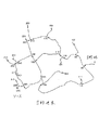
更なる例証および説明のために、多様なルートの生成方法の比較的単純な実際の例を説明する。これは図7〜10において、示される。そして、これらの図は同じ縮尺および広がりで描かれたマップである。選択された例は、英国ケンブリッジから英国マンチェスターまでのルートである。 For further illustration and explanation, a relatively simple practical example of a variety of route generation methods is described. This is shown in FIGS. These figures are maps drawn at the same scale and spread. The example chosen is the route from Cambridge, UK to Manchester, UK.
第一ステップは、ケンブリッジから他の全ての点まで最良のルート(最小限のコスト)を含んでいる木を計算することである。これは、図7において、示される。
The first step is to compute the tree that contains the best route (minimum cost) from Cambridge to all other points. This is shown in FIG.
木は印刷のために単純化されており、その主要枝だけを示している。木全体の葉を入れると、このスケールでは、ほぼ完全にその土地を埋め尽くしてしまうからである。この種の木を計算する方法は、当該技術において、周知であり、ダイクストラのアルゴリズムおよびA*アルゴリズムを含む。 The tree has been simplified for printing, showing only its main branches. If you put the leaves of the whole tree, this scale will almost completely fill the land. Methods for computing this type of tree are well known in the art and include Dijkstra's algorithm and A * algorithm.
第二ステップは、他の全ての点からマンチェスターまでの最良の(最小限のコスト)ルートを含んでいる木を計算することである。これは、図8において、示される。 The second step is to compute the tree that contains the best (minimum cost) route from all other points to Manchester. This is shown in FIG.
第三ステップは、両方の木において、同じ方向に、すなわち、図7において、ケンブリッジから離れる方向へ、そして、図8において、マンチェスターの方へ、辿られる道を見つけることである。辿りの方向が重要であるので、そのような道は単に2本の木の重なりでない。結果として生じる道は、図9において、示される。 The third step is to find a path that is followed in both trees in the same direction, ie, away from Cambridge in FIG. 7, and towards Manchester in FIG. Such a path is not just an overlap of two trees, since the direction of tracing is important. The resulting path is shown in FIG.
第四ステップ(その出力が図10において、示される)は、最も長い道のチェーンを図9から選択し、図7のソース木を用いてケンブリッジへ戻るまで、そして、図8の目的地木を用いてマンチェスターに戻るまで、各チェーンの終端点を連結することにより、それぞれのチェーンから完全なルートを生成することから始まる。ルートはそれからそれらの良好性(重なり合うチェーンのコスト引く全てのルートのコスト)に従って並べられる。そして、この場合、我々は上位5個(良好性の順に0番から4番まで)を表示することを選択した。 The fourth step (whose output is shown in FIG. 10) selects the longest path chain from FIG. 9 and returns to Cambridge using the source tree of FIG. 7 and the destination tree of FIG. Start by generating a complete route from each chain by connecting the end points of each chain until you use it back to Manchester. The routes are then ordered according to their goodness (cost of overlapping chains minus cost of all routes). And in this case, we have chosen to display the top 5 (from 0 to 4 in order of goodness).
本実施例における最終ステップは、ユーザに関係情報を表示することである。たとえば、表1に示されるような情報である。
表1
Table 1
次に、多様ルート発生器および車両ナビゲーション・システムにおけるそのアプリケーションのより包括的な例について説明する。見出しは、便宜のために提供される。 A more comprehensive example of a multi-route generator and its application in a vehicle navigation system will now be described. Headings are provided for convenience.
<ルーティング木>
これらの役立つチェーンを見つけるために、我々はまず、Aからすべてのノードまでの、そして、すべてのノードからBまでのルートを見る。我々は、ダイクストラのアルゴリズムを用いてAからすべてのノードまでの最適ルートを計算し、これらが単一の木構造つまり、A(RTa)からのルーティング木に格納され得ることに気がつくことができる。その木では、各ノードまたはリンクは、最適ルートに沿って以前のものへのポインタを含む。図11は、このような木を示すために単純な例を示す。ノードまたはリンクは、その点までの最適ルートのコストを含むこともできる。この木は、局所的に最適でありAから離れるためによく整列配置される道を用いる傾向がある。「局所的に最適」であるとは、全体コストを低下させることができるルートを外れるマイナーな迂回路がないことを意味している。
<Routing tree>
To find these useful chains, we first look at the route from A to all nodes and from all nodes to B. We can use Dijkstra's algorithm to compute the optimal route from A to all nodes and notice that these can be stored in a single tree structure, ie the routing tree from A (RTa). In that tree, each node or link contains a pointer to the previous one along the optimal route. FIG. 11 shows a simple example to illustrate such a tree. A node or link can also include the cost of the optimal route to that point. This tree tends to use paths that are locally optimal and well aligned to leave A. “Locally optimal” means that there are no minor detours off the route that can reduce the overall cost.
次に、我々は、すべてのノードからB(RTb)までの最も最適なパスを格納する第2のルーティング木を計算する。この木は、局所的に速くかつBの方へ行くのに役立つ道路区分に有利に働く。そして、図12は図11において、示される例のための、得られた木を示す。 Next, we compute a second routing tree that stores the most optimal path from all nodes to B (RTb). This tree favors a road segment that is locally fast and helps to go towards B. And FIG. 12 shows the resulting tree for the example shown in FIG.
<木の合成(combining)>
今度は、我々は、両方の木において、同じ方向に用いられるノードのチェーンを見つけるために、2つのRTを合成する。これらのチェーンは、Aから移動して離れるのにおいて、そして、Bの方へ移動するために役立つ。このようなチェーンから完全なルートを生成するために、我々は、RTaを用いてチェーンの始めからAへとたどって戻り、RTbを用いてチェーンの端からBまで前進する。図11の例のための結果生じたルートは、図13に示される。このルートは、局所的に最適である。すなわち、AからBまで行くのに全体コストがより低くなる小さいずれは存在しない。チェーンからのこのようなずれがある場合には、チェーンはより低コストのそれたルートで形成されていたのだろうし、ルートのたどられた端からこのような脇道がある場合には、適切なルーティング木(RTaまたはRTb)が最適ではなかったのであろう。
<Combining wood>
This time we synthesize two RTs to find a chain of nodes used in the same direction in both trees. These chains serve to move away from A and move toward B. To generate a complete route from such a chain, we go back to A from the beginning of the chain using RTa and advance from the end of the chain to B using RTb. The resulting route for the example of FIG. 11 is shown in FIG. This route is locally optimal. That is, there is no small going from A to B that the overall cost is lower. If there was such a deviation from the chain, the chain would have been formed with a less expensive route, and if there was such a side street from the traced end of the route, it would be appropriate The correct routing tree (RTa or RTb) may not have been optimal.
これらのチェーンから生成されるルートが局所的に最適であるにもかかわらず、それらがグローバルには最適でない点に注意する。一般に、グローバルに最適なルートは1つだけある。それは単一のルーター(例えばダイクストラのアルゴリズム)によって、見つけられるものである。2番目に最適なルートは、通常 1番目に最適なルートの軽微なバリエーションであって、コスト僅かに増加しているだけである。例えば、町で始まり町で終わる3時間の車の旅において、計算された旅行時間に僅か何分かを追加する、脇道による何百もの小さいずれが潜在的に存在する。それら全て並べ替えると、3時間10分までの行程時間を有するルートを何百万も生成することになる。その後でようやく、我々は、町と町との間の非常に異なるルートを用いるものであって余分に12分要する第1の旅を見るかもしれない。この旅にも潜在的に何百万もの小さいバリエーションがある。それらはすべて、ほんのわずかだけ高コストであるが、局所的に最適である。もちろん、それが1,000,000番目に短いルートである場合であっても、それは、依然として完全に現実的な代替物であるかもしれない。というのは、見積行程時間は、多分±10分の誤差を有するからである。そして、我々が選択肢を提示される場合、我々は他の要因を考慮できる。例えば、我々がドライブするルートがどれくらい楽しいかとか、我々がそのルートにどれくらい慣れているかとか、この機会における財政的なコスト対時間の重要性とかである。 Note that even though the routes generated from these chains are locally optimal, they are not globally optimal. In general, there is only one route that is globally optimal. It can be found by a single router (eg Dijkstra's algorithm). The second best route is usually a minor variation of the first best route, with only a slight increase in cost. For example, in a three hour car trip that starts and ends in town, there are potentially hundreds of small ones by side roads that add only a few minutes to the calculated travel time. Rearranging all of them will generate millions of routes with journey times of up to 3 hours and 10 minutes. Only then may we see a first trip that uses a very different route between towns and takes an extra 12 minutes. There are potentially millions of small variations on this journey as well. They are all locally optimal, although only slightly more expensive. Of course, even if it is the 1,000,000th shortest route, it may still be a completely realistic alternative. This is because the estimated travel time will probably have an error of ± 10 minutes. And when we are presented with options, we can consider other factors. For example, how fun the route we are driving, how familiar we are with the route, and the importance of financial cost versus time at this opportunity.
もちろん、このようなチェーンは多くあるが、それらの数の上限はグラフ中のエッジの数である。しかし、それらは道路区分の重なり合うチェーン(それを我々は、台地と呼ぶ)の長さ(一般に、コスト)およびそのチェーンを用いる最適ルートのための道の長さ(コスト)によって、特徴付けられることが可能である。これのためのコスト情報はRTsデータにおいて、すでに利用できるので、これは代替ルートの良好性を評価する非常に効率的な方法である。我々は、適正な良好性関数を発見した。この関数は、グローバルに最適なものから下方への最良の多様ルートを順序づけるだけでなく、どれくらいの代替物が本当に役立つかについて確認するために無次元閾値を提供する。 Of course, there are many such chains, but their upper limit is the number of edges in the graph. However, they are characterized by the length of the overlapping chain of road segments (which we call the plateau) (generally cost) and the length of the road (cost) for the optimal route using that chain Is possible. Since the cost information for this is already available in the RTs data, this is a very efficient way to evaluate the goodness of alternative routes. We have found a good goodness function. This function not only orders the best diverse routes down from the globally optimal one, but also provides a dimensionless threshold to see how many alternatives are really useful.
この方法を用いることにより、我々は、ダイクストラのアルゴリズムを二回実行することにより支配される時間で、AからBまでのN個の最良の多様な代替ルートを計算できる。我々は、ダイクストラのアルゴリズムを実行するよりも非常に少ない時間で、このようなルートを数千も評価し順序づけることができる。但し、通常は、良好性要因が閾値を上回るものは1ダース未満である。 By using this method, we can compute the N best diverse alternative routes from A to B in a time dominated by running Dijkstra's algorithm twice. We can evaluate and order thousands of such routes in much less time than executing Dijkstra's algorithm. However, it is usually less than a dozen if the goodness factor exceeds the threshold.
周知の単一のルーター(AからBへの最も短い単一のパス)のいくつかの実施において、ダイクストラのアルゴリズムのバリエーションを用いることは、望ましいかもしれない。これらは、より良い状態のノードまたはエッジを探索するために、または、より早く終了するために、または主要道路だけを調べるために、または、同時にソースおよび目的地から外へ調査するために、特別なヒューリスティックを用いる。それらは、より速く動作したり、メモリの使用量を減らすために、これを行う。台地を見つけるためにRTを合成する我々の方法がRTsがどのような方法で計算されたかということとは無関係であることを理解すべきである。したがって、これらのバリエーションが適切であれば、それらのより良い実行時間またはメモリ使用特性を利用しつつ、多様な代替ルートを産生するために、我々の方法をそれらに適用できる。 In some implementations of a known single router (the shortest single path from A to B), it may be desirable to use a Dijkstra algorithm variation. These are special for exploring nodes or edges in better condition, or to finish earlier, or to examine only the main road, or to investigate out of the source and destination at the same time Use heuristics. They do this to work faster or reduce memory usage. It should be understood that our method of synthesizing RT to find plateaus is independent of how RTs were calculated. Thus, if these variations are appropriate, our method can be applied to them to produce a variety of alternative routes while taking advantage of their better execution time or memory usage characteristics.
<コスト関数>
最良の多様な代替ルート(選択ルートchoice route)を計算するために用いられるコスト関数は、周知の要因のいずれでも組み込むことができる。それは、時間および期間に対して敏感であってもよく、リアルタイムまたは歴史的な交通情報を組み込むことができ、利用者の好みを考慮することができ、財務情報(例えば道路使用料金)を用いることができる。
<Cost function>
The cost function used to calculate the best variety of alternative routes (choice route choice route) can be incorporated with any of the well-known factors. It may be sensitive to time and duration, can incorporate real-time or historical traffic information, can take into account user preferences, and use financial information (eg road usage charges) Can do.
しかしながら、好ましい実施例において、我々は、基本的なコスト関数を用いる。それは、殆ど時間に重みをおき、距離については余り参酌しない。これは、人がAからBまで行くために考慮するかもしれないルートの殆どを生成する。次に、我々は、ルートプランナにおいて、それらに各々のためのデータを提示することができる。そのデータは、時間、距離、財政的なコスト、渋滞情報およびその他の計算しうるあらゆるパラメータ(ターン数、安全性等)を与えるものである。我々はこれらを、1日の異なる時間、異なる曜日、異なるタイプの車両のすべてに対して非常に簡単に計算することができる。なぜならば、我々は、第一ステップにおいて、見つけた一握りの選択ルートだけを考慮しさえすればよいからである。いまや我々はユーザをループに入れたので、彼らはすばやく各ルートがどこに行くかを見ることができ、彼らが異なるコスト基準にどのような重みを与えることを望むかに基づいて、彼らを決定できる。 However, in the preferred embodiment we use a basic cost function. It puts a lot of weight on time and doesn't really care about distance. This generates most of the routes that a person may consider to go from A to B. Then we can present them data for each in the route planner. The data gives time, distance, financial costs, traffic jam information and any other parameters that can be calculated (number of turns, safety, etc.). We can calculate these very easily for all of the different times of the day, different days of the week and different types of vehicles. This is because we only have to consider in the first step only a handful of selected routes we find. Now that we have put the users in a loop, they can quickly see where each route goes and can determine them based on how they want to give different cost criteria .
我々は、道路利用者課金があたりまえになれば、これが特に重要になると思っている。なぜならば、すべての旅に対して、そしてもちろんすべてのユーザに対して正しい方法で時間、距離および費用負担のバランスをとることは可能でないからである。同じ日の同じユーザさえ、彼らがその旅を終えるための固定期限を有するかどうか、疲れてきているかどうか、または、ちょうど現金が不足したかどうかによって、優先するものが異なるかもしれない。彼らは、かなり短い非高速道路ルートを通常好むかもしれないが、代替物が多くのターンを伴う場合、彼らは気分を変えるかもしれない。 We think this will be particularly important if road user billing becomes commonplace. This is because it is not possible to balance time, distance and cost burden in the right way for every trip and of course for every user. Even the same users on the same day may have different priorities depending on whether they have a fixed deadline to finish their journey, whether they are getting tired, or just run out of cash. They may usually prefer fairly short non-highway routes, but they may change their mood if the alternative involves many turns.
<選択肢提示>
周知のルート・プランナに関する他の問題は、ユーザがいくつかの他のルートがなぜ推奨されなかったかについて疑問に思うかもしれないということである。彼らに代替ルートをそれらの特徴とともに示すことによって、ユーザがそれらの代替ルートがどのように最良のものに匹敵するかについて見て、適正な選択をすることは、容易である。例えば、いつものルートはいつになくひどい渋滞になるかもしれない、あるいは、バイパスの建設のため代替ルートが好ましくなったかもしれない。
<Option presentation>
Another problem with known route planners is that users may be wondering why some other routes were not recommended. By showing them alternate routes along with their characteristics, it is easy for the user to see how those alternate routes are comparable to the best and make the right choice. For example, the usual route may never have been terribly congested, or an alternative route may have become preferred due to the construction of a bypass.
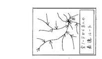
ルート選定(route planning)ツールにおいて、我々は、異なる色を用いて異なるルートを強調することができ、各ルートについて時間、コストなどの関連した詳細を有するテキストボックスを提示することができる。先に説明されたケンブリッジからマンチェスターまでのルートに対するテキストボックスの例が図14に示される。マップ上のルートを選択すればテキストボックス内の関連した線を強調することができ、テキストボックスにおいて、ある線を選択すればマップ上の関連したルートを強調することができるであろう。このようにして、ユーザは、我々が与えることのできるできるだけ多くの情報でもってルートを選択できる。 In a route planning tool, we can highlight different routes using different colors and present a text box with relevant details such as time, cost, etc. for each route. An example text box for the previously described Cambridge to Manchester route is shown in FIG. Selecting a route on the map will highlight the associated line in the text box, and selecting a line in the text box will highlight the associated route on the map. In this way, the user can select a route with as much information as we can give.
ルート選定ツールにおいて同時に選択ルートを提示する代わりに、我々は、他のユーザーインターフェースを考慮できる。例えば、ルート内(en-route)ガイダンスとしては、我々は、代替物を示すマップでドライバを混乱させたくない。むしろ、行程内で選択が行われることができる箇所(それを、我々は選択点と呼ぶ)を計算し、彼らがその選択点に接近するときにドライバに知らせる。ケンブリッジからマンチェスターへの6本の最善ルートの例に対しては、ドライバは、彼らの旅の間、多くても3回選択肢が提示される。更に、これらは、利用可能な情報の関連サブセットとともに提示されることができる。それらは、おそらくジャンクション図表として、どちらかといえば図15に示したような沿道のジャンクション看板のように、提示されることができる。この種の図表は、自動車のナビゲーション・システムにおいて、よく使用されており、最適ルート上にとどまるためにとるべき正しいターンをドライバに示す。選択点に接近するとき、我々のシステムは異なる。我々は、最適ルートと強調された他のあらゆる選択ルートの両方を有するジャンクション図表を示す。我々は、これを、用いられた道の概要、彼らの目的地までの相対時間、財政的なコスト等の情報で強化する。これらは、道路標識の形で示されることができ(そして、これ以上気をそらせるものであってはならない)、音声合成を用いて読出しすることもできる。それは「ロータリーで、M6およびM56用の第1の出口を出てください。あるいは、10分間長いけれども7ポンド安くするために、M1およびA6プライム2用の第2の出口を出てください”といった形をとることができる。交通情報が考慮された場合であってユーザが最適ルートがなぜ彼らが予想したものでないかについて疑問に思っているかもしれない場合に、特に役立つであろう。保存された時間またはコストは、これを彼らに明らかにする。 Instead of presenting the selected route at the same time in the route selection tool, we can consider other user interfaces. For example, as en-route guidance, we do not want to confuse the driver with a map showing alternatives. Rather, it calculates where in the journey a selection can be made (we call it a selection point) and informs the driver when they approach that selection point. For the example of the six best routes from Cambridge to Manchester, drivers are offered at most three choices during their journey. Furthermore, they can be presented with a relevant subset of available information. They can be presented, perhaps as a junction chart, rather like a roadside junction sign as shown in FIG. This type of chart is commonly used in car navigation systems and shows the driver the correct turn to take to stay on the optimal route. Our system is different when approaching the selection point. We show a junction diagram with both the optimal route and any other selected route highlighted. We enhance this with information such as an overview of the roads used, the relative time to their destination, and financial costs. These can be shown in the form of road signs (and should not be distracted any more) and can also be read out using speech synthesis. It's a form like "Take the first exit for M6 and M56 at the roundabout. Or take the second exit for M1 and A6 Prime 2 to make it 10 minutes long but 7 pounds cheaper" Can be taken. This will be especially useful when traffic information is considered and the user may be wondering why the optimal route is not what they expected. Saved time or cost makes this clear to them.
選択ルート(Choice Routes) が一旦わかれば、ソース・リンクから目的地リンクまで少数の選択ルートをたどることによって、選択点(Choice Points)自体を発見するのは容易である。我々はソース・リンクから始める。そして、それはあらゆる選択ルートの初まりで発見される。あらゆる選択ルート上の次のリンクが同じである場合、我々はそれへ移動する。次のリンクがルートで異なる場合、我々は選択点に達しているので、あたかも我々がちょうど今再びソース・リンクから始めたかのように、各ルートを別個にたどる。各ルートが目的地リンクに達したとき、我々は終了する。我々は、旅を開始するときに選択点の全てを計算できる、または、常に少なくとも1の選択点を前もって知るように保ちつつ、行く道中で、それらを計算できる。 Once the Choice Routes are known, it is easy to find the Choice Points themselves by following a few selected routes from the source link to the destination link. We start with a source link. And it is discovered at the beginning of every selected route. If the next link on every selected route is the same, we move to it. If the next link is different in the route, we have reached the selection point, so we will follow each route separately as if we just started again from the source link. When each route reaches the destination link, we are finished. We can calculate all of the selected points when we start the journey, or we can calculate them on the way to go, always keeping in mind at least one selected point in advance.
選択点を計算するために用いられることが可能である他の方法がある。例えば1つの選択ルートにより用いられたリンクの全てをマークしする。そして、どこで選択ルートが、マークされたノードからマークされていないノード(選択点)へ変更され、そして、また、マークされていないノードへ変更(収束点)されるのかに注目して、他の各選択ルートをマークする。これらの方法のいずれも選択点を決定するために用いられることができ、アプリケーションの正確な必要性に従って選択されることができる。 There are other methods that can be used to calculate the selection points. For example, mark all of the links used by one selected route. And note where the selected route is changed from a marked node to an unmarked node (selection point) and also to an unmarked node (convergence point) Mark each selected route. Any of these methods can be used to determine the selection point and can be selected according to the exact needs of the application.
<建設的、非破壊的>
我々の方法の重要な特性は、それが建設的であり、同時にすべての良い道を見つけ、非常に良い重みを用いて、しかも、個々の道リンクのコスト要素を盲目的に変える必要なく、それらの道を評価するということである。重みまたは個々のコスト要素を変えて最も最適なルートをあまり最適ではなくさせる方法は、その他の未知の良いルートの最適性を低めなかったかどうかわからない。したがって、それは決して見つからない。
<Constructive and non-destructive>
An important characteristic of our method is that it is constructive and at the same time finds all good roads, uses very good weights, and without having to blindly change the cost elements of individual road links It is to evaluate the way. It is not known whether changing the weights or individual cost factors to make the most optimal route less optimal is not reducing the optimality of other unknown good routes. Therefore it is never found.
我々は、この種の方法で我々の方法が第1に発見されるべきものであると思っている。なぜならば、我々の調査において、見つけた他のすべてのものが重みまたは個々の道要素を用いるコストの変更を伴うからである。以前に見つかったルートで用いられた一つ以上の道要素を禁止すること(人工的にそれらに無限のコストを与えることに等しい)によって、動作するものさえある。 We believe our method should be discovered first in this kind of method. Because in our study, everything else we find involves a change in weight or cost using individual path elements. Some even work by prohibiting one or more road elements used in previously found routes (equivalent to artificially giving them infinite cost).
<道グラフの表示>
重み付けをされた有向グラフのために用いられることが可能である様々な表示がある。例えば道路網のために、我々は、ジャンクションをグラフにおけるノードとして、ジャンクション間の道リンクをグラフにおけるエッジとして表すかもしれない。道を辿るコスト(例えばジャンクション間の道のりを辿るためにかかる距離および平均時間)を表すために、我々は、エッジにコストを割り当てることができる。あるいは、ジャンクションを通過するコスト(例えば、まっすぐに進行するためにかかる時間または左折若しくは右折するためにかかる時間)を表すために、我々はノードに対して、そのノードに着くために用いられるエッジ及びそのノードを離れるために用いられるエッジに依存するコストを割り当てることができる。この表示の多くのバリエーションは可能である。そして、我々の方法はその全部に適用できなければならない。
<Display of road graph>
There are various displays that can be used for weighted directed graphs. For example, for a road network we may represent junctions as nodes in the graph and road links between junctions as edges in the graph. To represent the cost (e.g. such distance and the average time to follow the road junction-) following the road, you can assign a cost to the edge. Alternatively, to represent the cost of going through a junction (eg, the time it takes to travel straight or the time it takes to turn left or right), we use the edge used to get to that node and A cost can be assigned that depends on the edge used to leave the node. Many variations of this display are possible. And our method must be applicable to all of them.
この実施のために、我々は、ルーティング木を計算するために特に高速である表示を用いる。この表示は、ノードとして道ジャンクションを表さない。その代わりに、各エッジは片方向である。したがって、二方向の道(往復道)の伸びは2つのエッジ(各移動方向につき1つ)により表される。そして、これらは厳格にグラフのノードを形成する。これにより我々が移動方向ごとに異なる遅延をコード化することができる。そして、それは渋滞の時間に重要かもしれない。我々は、各エッジを「リンク」と言う。 For this implementation we use a display that is particularly fast to compute the routing tree. This display does not represent a road junction as a node. Instead, each edge is unidirectional. Thus, the extension of the bi-directional road (round trip) is represented by two edges (one for each direction of movement). These strictly form graph nodes. This allows us to code different delays for each direction of travel. And that may be important during times of traffic. We call each edge a “link”.
ジャンクションの特性をコード化するために、各リンクは、グラフにおいて、それから達することができる次のリンクへのポインタの組(集合)を有する。これらは、「次リンク」と呼ばれている。これらの次リンク・ポインタは、厳密にグラフのエッジである。第一のリンクから次のものへ移動するコスト(時間、距離、財政的なコストその他において、)は、このような各ポインタと関連づけられる。我々の実施は、1つのリンク・エッジの中間点から別のものの中間点へ移動するのにかかられる時間(次リンク時間)を用いることを選択する、しかし、他のものは、リンクの起点またはそれら終点を用いることを選択するかもしれない。結果に差はない。我々は、各リンクの長さ(「リンク距離」)を格納し、長さを加えて2で割ることによって、1つのリンクの中央から次のリンクの中央までの距離を計算する。このようにして、我々は、1つの「次リンク」において、ある長さの道を辿るコストおよびある特定の方向転換のためのジャンクションを用いるコストの両方をコード化した。それにより、あるソース・エッジまたはノードから他のエッジまたはノードまでのルートの全てを計算することが特に効率的なものとなる。 To encode the junction characteristics, each link has a set of pointers to the next link from which it can be reached in the graph. These are called “next links”. These next link pointers are strictly the edges of the graph. The cost of moving from the first link to the next (in time, distance, financial costs, etc.) is associated with each such pointer. Our implementation chooses to use the time it takes to move from one link edge midpoint to another (next link time), but the other is the link origin Or you may choose to use those endpoints. There is no difference in the results. We calculate the distance from the center of one link to the center of the next link by storing the length of each link (“link distance”), adding the length and dividing by two. In this way, we are in the one "next link", by coding both cost using junction for cost and certain turning follow the path of a certain length. This makes it particularly efficient to compute all of the routes from one source edge or node to another edge or node.
ソース・リンクからの最適ルートよりもむしろ特定の目的地リンクへの最適ルートを計算するために、我々は各リンクにPrevLinksの集合を与える。それは、そのリンクへすべての可能な先行リンク(すなわちそこへ入れる道の部分)から入るコストをコード化する。あらゆるPrevlinkは対応するNextLinkを有するので、幾らかの冗長がある。したがって、我々はいくつかの表示よりも多くのメモリを用いるが、実行時間は少ない。 In order to calculate the optimal route to a particular destination link rather than the optimal route from the source link, we give each link a set of PrevLinks. It encodes the cost of entering that link from all possible predecessor links (ie, the portion of the way into it). Every Prevlink has a corresponding NextLink, so there is some redundancy. Therefore, we use more memory than some displays, but run less.
図16は、脇道がジャンクションの方へ一方通行である道ジャンクションを示す。Aと記された道部分は2つのリンク1および3により表される。それは対面(2方向)道路だからである。同様に、道部分Bは、2つのリンク2および4により表される。道部分Cは、ジャンクションへ向かう一方通行であるので、1つのリンク5だけで表される。
FIG. 16 shows a road junction where the side road is one-way towards the junction. The road portion marked A is represented by two
さて、道部分A上のジャンクションの方へ移動している車両は、部分Bだけに続くことができる。そのため、1つの「次リンク」(矢印)だけがリンク1から出ており、そのリンクはリンク2を指している。同様に、道部分B上のジャンクションの方へ移動している車両は、部分Aに続けることができるだけである。そのため、リンク4から次リンクが出ており、それはリンク3を指している。ジャンクションの方へ道部分Cを移動している車両は、部分Aまたは部分Bのどちらかに折れてジャンクションから離れることができるので、対応するリンク5はそれから出ている次リンクを2つ有する。それらはリンク2,3を指している。ここでの重要な要因は、NextLinksが、それらが向かうリンクからではなく、それらが出ているリンクから、列挙されることができるということである。
Now, a vehicle moving towards a junction on road part A can only follow part B. Therefore, only one “next link” (arrow) exits from
PrevLinksは、次リンクの逆であって、ここでも、それらが出ているリンクから列挙される。それらは、車両がそこからこのリンクに入るかもしれないリンクを示す。例えば、車両は、このジャンクションで道部分BまたはCから道部分Aに入るかもしれないので、リンク3は、リンク4およびリンク5を指すPrevLinksを有する。 PrevLinks is the inverse of the next link, again enumerated from the links they exit. They indicate the links from which the vehicle may enter this link. For example, link 3 has PrevLinks pointing to link 4 and link 5 because the vehicle may enter road portion B from road portion B or C at this junction.
このリンク・データは一組のファイルすなわちファイルの集合(各ファイルにはタイプ別の情報)として格納される。それらは、効率的にアクセスできるようメモリに簡単にマップされることができる。各リンクは単純な整数ID(長さ32ビット、0から順に大きい数字)を与えられる。そしてそれは、さまざまなファイルへのオフセットとして用いられる。我々は、例としてリンクID435を用いる。リンク435の長さは、ファイルLinkDistanceの43第五の16ビット語で見つかる。それは、16ビットのメートル単位の長さとしてコード化されている。NextLinksであるリンク435から達することができるリンクは、NextLinksと呼ばれるファイルに32ビットのリンクIDを有する。ファイルNextLinkIndexにおいて、43第五の32ビット語はファイルNextLinksにオフセットを与える。そのファイルには次リンクのlinkIDsが隣接して見つかる。それらの数は、ファイルNextLinkCountにおいて、43第五の8ビット語で見つかる。特定の次リンクへ移動するためにかかる時間は、ファイルNextLinkTimeにおいて、与えられる。NextLinkIndexおよびNextLinkCountの見出しも付けられている。さらに、我々は、リンクの数(nLinks)、次リンクの数(nNextLinks)およびPrevLinksの数(nPrevLinks)を格納するマスター・ファイルを加える。一般に、nPrevLinks=nNextLinksである。 The link data is stored as a set of files, that is, a set of files (information on each type for each file). They can be easily mapped into memory for efficient access. Each link is given a simple integer ID (32 bits in length, starting with 0 in order). And it is used as an offset to various files. We use link ID 435 as an example. The length of link 435 is found in the 43th fifth 16-bit word of the file LinkDistance. It is encoded as a 16-bit metric length. A link that can be reached from link 435 which is NextLinks has a 32-bit link ID in a file called NextLinks. In the file NextLinkIndex, the 43rd fifth 32-bit word gives an offset to the file NextLinks. LinkIDs of the next link are found adjacent to the file. Those numbers are found in the 43th fifth 8-bit word in the file NextLinkCount. The time taken to move to a specific next link is given in the file NextLinkTime. There are also headings for NextLinkIndex and NextLinkCount. In addition, we add a master file that stores the number of links (nLinks), the number of next links (nNextLinks), and the number of PrevLinks (nPrevLinks). In general, nPrevLinks = nNextLinks.
これまでのファイル定義を示す。ファイル内の要素の数は、ファイル名の後、角括弧内に示され、その後には、各要素のタイプが続いている。 The file definition so far is shown. The number of elements in the file is shown in square brackets after the file name, followed by the type of each element.
ファイル記述:
Master[3]:INT32:リンクの数(nLinks)と、次リンクの数(nNextLinks)と、前リンクの数(nPrevLinks)とを格納し、そして、おそらく、ファイルがどのようにして生成されたかについてのその他のトップ・レベル情報も格納している。これまでのところ、全3フィールドは、INT32である。
File description:
Master [3]: INT32: Stores the number of links (nLinks), the number of next links (nNextLinks), the number of previous links (nPrevLinks), and possibly about how the file was generated Other top level information is also stored. So far, all three fields are INT32.
すべての他のファイルは、単純アレーである。リンクは、そのリンク・インデックス、すなわち0とnLinks−1との間の整数により定義される。それは、長さが[nLinks]の倍数であるファイルに格納されたアレーの全てを指し示している。
NextLinkIndex[nLinks]:INT32:次リンクが見つけられるNextLinksファイルにおけるオフセットを格納する。
NextLinkCount[nLinks]:INT8:次リンクの数を格納する。
NextLinks[nNextLinks]:INT32:1つのリンクからアクセスされることができる次リンク(インデックスによって、)を格納する。
PrevLinkと呼ばれている同様の1組の3つのファイルは、目的地ルーティングのためのルーティング木をコード化する。
PrevLinkIndex[nLinks]:INT32:次リンクがあるNextLinksファイルにおけるオフセットを格納する。
PrevLinkCount[nLinks]:INT8:リンクの数を格納する。
PrevLinks[nPrevLinks]:INT32:1つのリンクからアクセスされることができるリンク(インデックスによって、)を格納する
LinkType[nLinks]:INT8:道リンクのタイプ。0は速い、255は遅い。
NextlinkTime[nNextlinks]:INT32:このリンクの中央から次リンクの中央まで行くのにかかる増加時間(ミリ秒)(ジャンクション遅延を含む)。
PrevLinkTime[nPrevlinks]:INT32:前のリンクの中央からこのリンクの中央まで来るのにかかる増加時間(ミリ秒)(ジャンクション遅延を含む)。
LinkDistance[nLinks]:INT16:このリンクを用いたときの増加距離(メートル)。
All other files are simple arrays. A link is defined by its link index, an integer between 0 and nLinks-1. It points to all the arrays stored in a file whose length is a multiple of [nLinks].
NextLinkIndex [nLinks]: INT32: Stores the offset in the NextLinks file where the next link can be found.
NextLinkCount [nLinks]: INT8: Stores the number of next links.
NextLinks [nNextLinks]: INT32: Stores the next link (by index) that can be accessed from one link.
A similar set of three files called PrevLink encodes a routing tree for destination routing.
PrevLinkIndex [nLinks]: INT32: Stores the offset in the NextLinks file where the next link is.
PrevLinkCount [nLinks]: INT8: Stores the number of links.
PrevLinks [nPrevLinks]: INT32: LinkType [nLinks]: INT8: Type of road link that stores links (by index) that can be accessed from one link. 0 is fast and 255 is slow.
NextlinkTime [nNextlinks]: INT32: Increase time (in milliseconds) taken from the center of this link to the center of the next link (including junction delay).
PrevLinkTime [n Prevlinks]: INT32: Increased time (in milliseconds) taken from the center of the previous link to the center of this link (including junction delay).
LinkDistance [nLinks]: INT16: Increased distance (in meters) when using this link.
<ルーティング、アルゴリズム、ソース木>
所定のリンクから他の全てのリンクまでの最小コスト・ルート(ソース・ルーティング木)を造るために用いるルーティング・アルゴリズム(ダイクストラのアルゴリズムの一バージョン)は、以下の通りである。
<Routing, algorithm, source tree>
The routing algorithm (one version of Dijkstra's algorithm) used to build the least cost route (source routing tree) from a given link to all other links is as follows.
そのリンクに達するためにこれまでに見つかった最小限のコストであるmin−costを有するすべてのリンクから始める。そのリンクの原点(min−costがゼロである)以外のすべてのリンクについてそれを無限とする。活動ノード(我々がそれらの出リンクの全てをまだ探索したわけではないもの)の可変長リストを造る。最初にこのリストにソース・リンクだけを入れる。 Start with all links that have min-cost, the lowest cost found so far to reach that link. Make it infinite for all links other than the link origin (min-cost is zero). Build a variable-length list of active nodes (those we have not yet searched all of their outgoing links). First put only source links in this list.
これを繰り返す。
アクティブリストが空であれば、我々は終了しており、リターンする。
Repeat this.
If the active list is empty, we are done and return.
そうでなければ、アクティブリンクのリストから第1のアクティブリンクを削り、それをlinkPと呼ぶ。それは、我々がそれに着くことができることを知っている最小コストcostPを有する。出リンクlinkPNごとに、linkPからlinkNへ行く増分費用costPNを加える。そして、それがその出リンクに関して格納された最小コスト(costN)未満かどうか確かめる。もしもそうであるならば、costNを低い値で更新し、linkPを参照するためにlinkNのバックポインタを更新し、linkNをアクティブリンクのリストに加える(それがまだそこにない場合)。 Otherwise, remove the first active link from the list of active links and call it linkP. It has a minimum cost costP that we know can get to it. For each outgoing linkPN, add the incremental cost costPN going from linkP to linkN. It then checks to see if it is less than the stored minimum cost (costN) for that outgoing link. If so, update costN with a low value, update linkN's back pointer to reference linkP, and add linkN to the list of active links (if it is not already there).
このアルゴリズムが終わると、我々はルーティング木を構築したことになる。 When this algorithm is over, we have built a routing tree.
<ルーティング木の格納>
我々の実施例において、我々は前に計算されたルーティング木を再利用したいかもしれないので、我々は3つのファイルとしてそれぞれをファイリングシステムに格納する。異なる木は、各ファイル上の後置整数値<n>を用いることにより区別される。例えば、TTBackIndex1には、木1のためのバックポインタが入っている。規約により、現在選択されているソースおよび目的地リンクのための木は、nが0および1であるファイルに格納される。ここでも、ファイルの長さは、ファイル名の後、角括弧内に示されている。
<Storing the routing tree>
In our example, we may want to reuse the previously computed routing tree, so we store each as three files in the filing system. Different trees are distinguished by using a postfix integer value <n> on each file. For example, TBackIndex1 contains a back pointer for
ファイル記述:
TTMaster<n>[4]:一連のINT32:nLinks、fromSource(0=目的地、1=ソース)rootLinkIndex、rootSubnodeIndex。
TTBackIndex<n>[nLinks]:INT32:木<n>について、最も低いコストでこのリンクに到達するために用いられたリンク。次または前の(ソースまたは目的地)木のための作業。
TTMinCost<n>[nLinks]:INT32:木<n>について、このリンクに到達するために見つかった最小限のコスト。
File description:
TTMaster <n> [4]: A series of INT32: nLinks, fromSource (0 = destination, 1 = source) rootLinkIndex, rootSubnodeIndex.
TTBackIndex <n> [nLinks]: INT32: The link used to reach this link at the lowest cost for the tree <n>. Work for the next or previous (source or destination) tree.
TTMinCost <n> [nLinks]: INT32: Minimum cost found to reach this link for tree <n>.
<最適ルートをたどる(トレースバックする)こと>
ソース・リンクlinkAから目的地リンクlinkBまでの最適ルートを見つけるために、我々は、TTBackIndex0ファイルを用いなければならないだけである。例えば、linkBがID678,123を持っていたと仮定する。最適ルートに沿って我々をlinkBに導いたリンクは、ファイルTTBackIndex0において、オフセット678,123で見つかる。このリンクがID1,456,789を有していたと仮定する。最適ルートに沿って我々をこれに導いたリンクは、ファイルTTBackIndex0において、オフセット1,456,789で見つかる。ファイルから抽出されたリンクIDがソース・リンクlinkAのリンクIDに合致するまで、我々はこれを繰り返し続ける。そうすると、我々は、最適(最も短い)パスのリンクIDの全てを逆順に抽出したことになる。一旦ダイクストラのアルゴリズムが終わってしまうと、これは最短パスを抽出する一般的な方法である。
<Follow the optimal route (trace back)>
In order to find the optimal route from source link linkA to destination link linkB, we only have to use the TTBackIndex0 file. For example, assume that linkB has IDs 678 and 123. The link that led us to linkB along the optimal route is found at offset 678,123 in the file TTBackIndex0. Assume that this link had ID 1,456,789. The link that led us to this along the optimal route is found at offset 1,456,789 in the file TTBackIndex0. We will continue this until the link ID extracted from the file matches the link ID of the source link linkA. Then, we have extracted all the link IDs of the optimal (shortest) path in reverse order. Once Dijkstra's algorithm is over, this is a common way to extract the shortest path.
この抽出法は、活動ノードが全くなくなるまでルーティング・アルゴリズムを走らせたのであれば、linkAからグラフ中の他のいかなるリンクlinkCまでの最短パスを見つけるためにも機能する。ルーティング・アルゴリズムが早く終了された場合、我々はグラフ中のノードのサブセットへの最適ルートを見つけるために木を用いることができるだけである。 This extraction method works to find the shortest path from linkA to any other link linkC in the graph if the routing algorithm is run until there are no active nodes. If the routing algorithm is finished early, we can only use the tree to find the best route to a subset of nodes in the graph.
<ルーティング・アルゴリズム、目的地木>
すべてのリンクから所定のリンク(目的地ルーティング木)までの最小コスト・ルートを造るために我々が用いるルーティング・アルゴリズム(ダイクストラのアルゴリズムのバージョン)は、以下の通りである。
<Routing algorithm, destination tree>
The routing algorithm we use to build the least cost route from all links to a given link (destination routing tree) (Dijkstra's algorithm version) is as follows.
そのリンクから目的地リンクまで移動するためのそれまでに見つかった最小限のコストであるmin−costを有するすべてのリンクから始める。ルートの目的地(目的地リンク)(min−costがゼロである)以外のすべてのリンクについて、それを無限大にする。活動ノード(我々がまだそれらの入リンクの全てを探索し終えていないもの)の可変長リストを造る。最初はこのリストに目的地リンクデータのみを読み込む。 Start with all links with min-cost, the minimum cost found so far to travel from that link to the destination link. For all links other than the destination of the route (destination link) (min-cost is zero), make it infinite. Build a variable length list of active nodes (those we have not yet explored all of those incoming links). Initially, only the destination link data is read into this list.
これを繰り返す。
アクティブリストが空である場合、我々は終了したので、リターンする。そうでなければ、アクティブリンクのリストから第1のアクティブリンクを削除し、それをlinkQと呼ぶ。それは、我々が目的地に着くことができることがわかっている最小コストcostQを有する。入リンクlinkNQごとに、linkNからlinkQへ行く増分費用costNQを加える。そして、それが入リンクと共に格納されている最小コスト(costN)未満かどうか確かめる。もしもそうであるならば、costNをそのより低い値に更新し、linkQを参照するためにlinkNのバックポインタを更新し、アクティブリンク)のリストに、linkNを加える(それがまだそこにない場合)。
Repeat this.
If the active list is empty, we are finished and return. Otherwise, remove the first active link from the list of active links and call it linkQ. It has a minimum cost costQ that we know we can get to our destination. For each incoming linkNQ, add the incremental cost costNQ going from linkN to linkQ. It then checks to see if it is less than the minimum cost (costN) stored with the incoming link. If so, update costN to its lower value, update linkN's back pointer to reference linkQ, add linkN to the list of active links (if it is not already there) .
このアルゴリズムが終了するとき、我々はルーティング木を造り終えたことになる。 When this algorithm ends, we have finished building the routing tree.
<最適ルートをたどる(トレースバックする)こと>
目的地木を用いてソース・リンクlinkAから目的地リンクlinkBへの最適ルートを発見するために、我々は、TTBackIndex1ファイルを用いなければならないだけである。例えば、linkAがID 238,345を持っていたと仮定する。linkAが最適ルートに沿って先行したリンクは、ファイルTTBackIndex1において、オフセット238,345で見つかる。このリンクがID 1,432,876を持っていたと仮定する。このリンクが最適ルートに沿って先行したリンクは、ファイルTTBackIndex1において、オフセット1,432,876で見つかる。我々は、ファイルから引き出されたリンクIDが目的地リンクlinkBのlinkIDに合致するまで、これを繰り返し続ける。そうして、我々は、最適(最も短い)パスのリンクIDの全てを正順(前進方向)に抽出する。一旦ダイクストラのアルゴリズムが終わっているならば、これは最短パスを引き出す一般的な方法である。
<Follow the optimal route (trace back)>
In order to find the optimal route from source link linkA to destination link linkB using the destination tree, we only have to use the TTBackIndex1 file. For example, assume that linkA had ID 238,345. The link that linkA preceded along the optimal route is found at offset 238,345 in the file TTBackIndex1. Suppose this link had ID 1,432,876. The link that this link preceded along the optimal route is found at offset 1,432,876 in file TBackIndex1. We keep repeating this until the link ID extracted from the file matches the link ID of the destination link linkB. Then, we extract all link IDs of the optimal (shortest) path in the normal order (forward direction). Once the Dijkstra algorithm is over, this is a common way to derive the shortest path.
なお、このパスは、上記セクションにおいて、ソース・ルーティング木から引き出されたものと同一となる。ダイクストラのアルゴリズムをソースノードから外側へと走らせるか、目的地ノードから内側へと走らせるかは重要でない。それはlinkAからlinkBまで単一の最短パス・ルートを常に見つける。しかしながら、ダイクストラのアルゴリズムの副産物であるルーティング木同士は、非常に異なる。それらが完全に共有する唯一のルートは、グローバルな最短パス・ルートである。 Note that this path is the same as that extracted from the source routing tree in the above section. It doesn't matter whether Dijkstra's algorithm runs from the source node to the outside or from the destination node to the inside. It always finds a single shortest path route from linkA to linkB. However, the routing trees that are a byproduct of Dijkstra's algorithm are very different. The only route that they fully share is the global shortest path route.
この抽出法は、活動ノードが全くなくなるまでルーティング・アルゴリズムを走らせたのであれば、グラフ中の他のいかなるリンクlinkCからlinkBまでの最短パスを見つけるためにも機能する。ルーティング・アルゴリズムが早く終了された場合、我々はグラフ中のノードのサブセットへの最適ルートを見つけるために木を用いることができるだけである。 This extraction method works to find the shortest path from any other link linkC to linkB in the graph if the routing algorithm is run until there are no active nodes. If the routing algorithm is finished early, we can only use the tree to find the best route to a subset of nodes in the graph.
<ルーティング木の合成(combining)>
一旦我々がソース・リンクlinkAからの木RTaおよび目的地リンクlinkBまでの木RTbを計算してしまうと、我々は豊富なコスト情報も持つことになる。
<Combining routing tree>
Once we compute the tree RTa from the source link linkA and the tree RTb to the destination link linkB, we will also have a wealth of cost information.
例えば、グローバルな最適ルートに沿ってlinkAからlinkBへ行くコストを見つけるために、我々は、目的地ルーティング木のための最小コストが入っているTTMinCost1ファイルにおいて、オフセット<linkA>を見る。 For example, to find the cost of going from linkA to linkB along the global optimal route, we look at the offset <linkA> in the TTMinCost1 file that contains the minimum cost for the destination routing tree.
我々は、ソース・ルーティング木のための最小コストが入っているTTMinCost0ファイルにおいて、オフセット<linkB>を見ることもできる。この値は、同じである。 We can also see the offset <linkB> in the TTMinCost0 file that contains the minimum cost for the source routing tree. This value is the same.
さて、我々が他のリンクlinkCに興味がある場合にはどうだろうか。ファイルTTMinCost1におけるオフセット<linkCのコスト>でのコストは、linkCから目的地linkBへの最小限コスト・ルートのコストである。ファイルTTMinCost0におけるオフセット<linkC>でのコストは、ソース・リンクlinkAからlinkCへの最小限コスト・ルートのコストである。これらの2つの量を合計すれば、我々はlinkAからlinkCを経てlinkBまでの最小限コスト・ルートのコストを見つけたことになる。 Now what if we are interested in other links linkC? The cost at the offset <cost of linkC> in the file TTMinCost1 is the cost of the minimum cost route from linkC to the destination linkB. The cost at offset <linkC> in file TTMinCost0 is the cost of the minimum cost route from source link linkA to linkC. Summing these two quantities, we have found the cost of the minimum cost route from linkA to linkC to linkB.
したがって、更なる反復なしで、我々は、linkAからグラフ内の他の任意のリンクlinkCを経てlinkBへ行くコストを見つけてしまった。我々は、ファイルTTBackIndex0およびTTBackIndex1に入れられているバックポインタを用いることにより、表示または他のために最適ルートを素早くたどることもできる。これは非常に強力な結果である。なぜならば、我々は(経由するグラフ中のリンクと同数程度の)代替ルートの全体集合をそれらのコストとともに効果的に計算したからである。もちろん、これらは可能なルートの全てのうちの小さいサブセットにすぎない。なぜならば、それらは、linkAからlinkCまでグローバルに最適なルートをたどり、linkCからlinkBまでグローバルに最適なルートをたどることを強いられているからである。 Thus, without further iterations, we have found the cost of going from linkA to linkB via any other link linkC in the graph. We can also quickly follow the optimal route for display or otherwise by using the back pointers contained in the files TTBackIndex0 and TTBackIndex1. This is a very powerful result. This is because we have effectively computed the entire set of alternative routes (as many as the links in the route graph) along with their costs. Of course, these are just a small subset of all possible routes. This is because they are forced to follow a globally optimal route from linkA to linkC and a globally optimal route from linkC to linkB.
<台地>
いまや、我々は、ルートが唯一でないことに気がつく。いくつかのリンク、即ちlinkPおよびlinkQが、ある。そこにおいて、linkPを経由してlinkAからlinkBへ行くことは、linkQを経由してlinkAからlinkBへ行くのと全く同じルートを生成する。1のルーティング木(即ちソース・ルーティング木 RTa)におけるlinkPおよびlinkQ間のルートが他のルーティング木(RTb)におけるlinkPおよびlinkQ間のルートと同一のときに、これは起こる。すなわち、linkPおよびlinkQ間の道の区画は、両方の木によって、連続して用いられたわけである。
<Plateau>
Now we realize that the route is not the only one. There are several links: linkP and linkQ. In this case, going from linkA to linkB via linkP generates exactly the same route as going from linkA to linkB via linkQ. This occurs when the route between linkP and linkQ in one routing tree (ie, source routing tree RTa) is the same as the route between linkP and linkQ in the other routing tree (RTb). That is, the road segment between linkP and linkQ was used in succession by both trees.
これらはまさに、我々が多様な代替ルートの一部として興味がある道の「良い」チェーンである。それらは、両方の木において、連続的に現れるチェーンである。我々はそれらを、リンクが入って離れる道を比較することにより見つけることを試みることができ、あるいは、RTaおよびRTbからのコストの総和を用いることができる。 These are exactly the “good” chains of roads that we are interested in as part of various alternative routes. They are chains that appear continuously in both trees. We can try to find them by comparing the way the links enter and leave, or we can use the sum of the costs from RTa and RTb.
それらのチェーンは、最小コストルート上のlinkAからlinkBへチェーン内のリンクのいずれかを経由して行くコストが同じコストであることにより特定される。このために、我々はこのようなチェーンを台地と呼ぶ。なぜならば、それを構成するリンクに沿って、コストの総和が一定であるからである。 These chains are identified by the same cost going from link A to link B on the least cost route via any of the links in the chain. For this reason, we call such a chain a plateau. This is because the total cost is constant along the links constituting the link.
次の2つのサブセクションは台地の一部であるリンクを見つけるための代替方式を提供する。それらの方法は、コスト関数の特性、および当該方法を実施するメモリおよびプロセッサアーキテクチャに応じて、異なる効果を持っているかもしれない。これらの方法が、異なるグラフ表示、異なるフラグ格納手段、および異なるコスト関数特性に適合できることも、明らかである。 The next two subsections provide alternative ways to find links that are part of the plateau. These methods may have different effects depending on the characteristics of the cost function and the memory and processor architecture that implements the method. It is also clear that these methods can be adapted to different graphical representations, different flag storage means, and different cost function characteristics.
<合成コストから台地リンクを見つけること>
台地の全てを見つけるために、我々は、linkIDsの全てをスキャンする。それぞれのために、我々は、各木(RTaおよびRTb)において、BackIndexにより示されているリンクを見て、コストの総和が双方とも同じであるかどうか見る。それらが同じである場合、我々は台地の一部としてこのリンクにフラグを立てる。フラグは、通常通り、メモリマップ式ファイルに格納される。それは、TCFlags01と呼ばれ、1リンクにつき8ビットを入れている。それは、この手順の初めに初期化されて、すべてのビット集合を0にセット(フラグの設定解除)する。我々は、そのオフセットを有するリンクが台地の一部として特定されたかどうかを示すフラグとして、最下位ビット(bit7)を用いる。
<Finding plateau links from synthesis costs>
To find all of the plateaus, we scan all of the linkIDs. For each one, we look at the links indicated by BackIndex in each tree (RTa and RTb) to see if the sum of costs is both the same. If they are the same, we flag this link as part of the plateau. The flags are stored in a memory mapped file as usual. It is called TCFlags01 and has 8 bits per link. It is initialized at the beginning of this procedure and sets all bit sets to 0 (unsets the flag). We use the least significant bit (bit 7) as a flag to indicate whether a link with that offset has been identified as part of the plateau.
フラグのファイル定義を示す。ファイル内の要素の数は、ファイル名の後、角括弧内に示され、その後には、各要素のタイプが続いている。 Indicates the file definition of the flag. The number of elements in the file is shown in square brackets after the file name, followed by the type of each element.
ファイル記述:
TCFlags01[nLinks]:0および1で表されるRTを合成するときに、フラグとして用いられる一連のINT8。
一旦この走査が終了すると、我々はチェーン(bit7を用いる)の一部であるリンクの全てに、端の2つのリンクを除き、フラグを立てている。
File description:
TCFlags01 [nLinks]: A series of INT8s used as flags when synthesizing RTs represented by 0 and 1.
Once this scan is complete, we flag all links that are part of the chain (using bit 7) except for the two links at the end.
コスト値が整数である場合のみ、この方法は機能する。その結果、丸め誤差は我々が期待している同等性を損なわない。更に、木がいかなる順序で造られたとしても、木内のリンクを辿るためのコストが常に同じである場合のみにこの方法は働く。これは大概そのとおりであるが、例えば、リンク・コストが時間に依存するものであって、2本の木において、わずかに異なる時間に辿られる場合、この方法は機能しないだろう。したがって、バックポインタに基づく代替方式がその代わりに用いられなければならない。 This method only works if the cost value is an integer. As a result, rounding errors do not compromise the equivalence we expect. Furthermore, no matter what order the trees are built, this method only works if the cost to follow the links in the tree is always the same. This is mostly true, but this method will not work if, for example, the link cost is time dependent and is traced to slightly different times in the two trees. Therefore, an alternative scheme based on the back pointer must be used instead.
<バックポインタから台地リンクを見つけること>
台地の全てを見つけるために、我々は、すべてのlinkIDをスキャンする。linkIDの値、即ちlinkPごとに、我々は、そのリンクがソース木において、バックポインタを持っているかどうか見る。ソース・リンク以外のすべてのリンクは、有効ポインタを持っている。それがlinkQを指していると仮定する。そうすると、我々は、オフセットがID linkQであるTCFlags01ファイル内のバイトに指名ビット(即ちTCFlags01ファイルにおけるbit5)をセットすることによって、linkQをソースポインタを有するものとしてマークする。我々は、linkPが目的地木において、バックポインタを持っているかどうかも見る。もしそうならば、つまりlinkRならば、我々は、オフセットがID linkRであるバイトに、異なるビット(即ちTCFlags01ファイル内のbit4)をセットする。我々がbit4およびbit5でフラグのどちらかをセットする場合、我々はもう一方を見て、それもセットされている場合には、このリンクが台地の一部であることがわかるので、我々はコスト方法と同様に台地ビット(bit7)をセットすることもできる。
<Finding plateau links from the back pointer>
To find all of the plateau, we scan all linkIDs. For each linkID value, ie linkP, we see whether the link has a back pointer in the source tree. All links except the source link have a valid pointer. Suppose it points to linkQ. We then mark linkQ as having a source pointer by setting the nomination bit (ie bit 5 in the TCFlags01 file) to the byte in the TCFlags01 file whose offset is ID linkQ. We also see if linkP has a back pointer in the destination tree. If so, ie linkR, we set a different bit (ie bit 4 in the TCFlags01 file) in the byte whose offset is ID linkR. If we set one of the flags in bit4 and bit5, we look at the other and if it is also set we know that this link is part of the plateau so we The plateau bit (bit 7) can be set in the same manner as the method.
一旦この走査が完了すると、我々はここでも、チェーン(bit7を用いる)の一部である全部のリンクに、2つの端リンクを除いて、フラグを立てたことになる。 Once this scan is complete, we again flag all links that are part of the chain (using bit 7) except for the two end links.
<台地リンクを集めること>
我々は、今度は、チェーン自体を見つけて、それらの特徴を描写することが必要である。我々は、新たにリンクの全てを走査することによりこれを行う。
<Collecting plateau links>
We now need to find the chains themselves and describe their characteristics. We do this by scanning all of the new links.
リンクごとに、我々は、(bit7を用いて)それが台地の一部としてフラグを立てられたかどうか見るために調べる。そうであった場合には、我々はbit6を見てそれがすでに処理されたかどうか見る。そうでなかった場合には、処理されたものとしてそれにマークし(bit6を用いて)、遭遇するリンクが台地の一部としてマークされる限り、上記ソース木および目的地木内をたどる(トレースバックする)。我々はすべてのこのようなリンクをビット6を用いて処理されたものとしてマークするので、走査の後段階でそれらに再び遭遇しても、この台地では我々はどのリンクも処理しないだろう。 For each link we check to see if it was flagged as part of the plateau (using bit 7). If so, we look at bit 6 to see if it has already been processed. If not, mark it as processed (using bit 6) and follow the source and destination trees as long as the link encountered is marked as part of the plateau (trace back) ). We mark all such links as processed using bit 6, so if we encounter them again later in the scan, we will not process any links on this plateau.
このようにして台地を追跡するので、我々はそれ以後の使用ために台地についての情報、たとえば、その長さおよびそれを辿るコスト等の情報を集めることができる。しかし、この特定の実施例では、我々は最良のプラトー選択の基礎としてコストを用いるだけである。そのコストはTTMinCostファイルにすでに保存されているので、我々はそれらを再度計算する必要がない。むしろ、我々は、台地の端のlinkIDに注意する。linkIDpsはソースに最も近い台地の端である。そして、linkIDpdは目的地に最も近い台地の端である。我々がこうして見つけた台地ごとに、(可能ならば)我々は、1つのリンクを上記端からソースおよび目的地近傍まで延ばし、RTaまたはRTbのいずれかから調べられたそれらのリンクについて最小コストの差を計算する(台地が各木の接続部を形成しているので、結果は同一でなければならない)。これが、我々が台地を辿るためのコストとするものである。 Since track this manner plateau, we information about the plateau for use thereafter, for example, it is possible to collect information such as cost of following its length and the same. However, in this particular embodiment we only use cost as the basis for selecting the best plateau. Since the costs are already stored in the TTMinCost file, we do not need to calculate them again. Rather we note the linkID at the edge of the plateau. linkIDps is the edge of the plateau closest to the source. LinkIDpd is the edge of the plateau closest to the destination. For each plateau we found in this way, we extended (if possible) one link from the end to near the source and destination, and the difference in the minimum cost for those links examined from either RTa or RTb. (The results must be the same because the plateau forms a connection for each tree). This is the cost for us to follow the plateau.
<良好性の基準>
さて、スキャンするとき、我々は一般に、より短い台地を拒否し、より長いものを保つことを望む。また、我々は、あまり長くないルートの部分を形成する台地を支持することを望む。我々がケンブリッジからマンチェスターへ行く場合、我々は多分、スコットランドにある長い台地(それは道のある配列により時々形成される)には興味を起こさないだろう。
<Goodness criteria>
Now, when scanning, we generally want to reject shorter plateaus and keep longer ones. We also want to support a plateau that forms part of a route that is not too long. If we go from Cambridge to Manchester, we probably won't be interested in the long plateau in Scotland, which is sometimes formed by an array of roads.
より高い関心のある台地だけを選択するために、我々は「良好性」値を計算する。我々は我々が興味がある台地に対してそれがより高い値を持つようにアレンジしている。そうして、我々は、最も高いn個の良好性値を有する台地の端部リンクを記録する。ここで、nは、我々がおそらくユーザに表示したくなり得る数(即ち100)より大きい。良好性は、ルートの特性(例えば距離、財政的コスト、道のタイプ、ソースおよび目的地からの距離)のいずれかを用いて、いかなる方法でも計算されることができる。 In order to select only the plateaus of higher interest, we calculate a “goodness” value. We arrange it to have a higher value for the plateau we are interested in. Thus we record the end link of the plateau with the highest n goodness values. Here, n is greater than the number we may want to display to the user (ie 100). Goodness can be calculated in any way using any of the characteristics of the route (eg distance, financial cost, type of road, distance from source and destination).
この実施において、我々は、(最小コスト(mincost)を計算するために用いられるような)コストに良好性値の基礎をおくことを選ぶ。我々は、端間のコスト差がより大きい台地に対してより高い良好性を欲する。というのは、それらは、一致させられたルーティング・ツリーのより長い部分を表すからであり、それ故、linkAからlinkBまで行くのに局所的に役立つより長く伸びた道を表すからである。しかしながら、我々はまた、全体コストがより高いlinkAからlinkBまでのルートを形成する台地に対してはより低い良好性値が欲しい。 In this implementation we choose to base goodness values on costs (such as those used to calculate mincost). We want higher goodness for a plateau with a higher cost difference between the edges. This is because they represent the longer part of the matched routing tree and therefore represent a longer stretched path that serves locally to go from linkA to linkB. However, we also want a lower goodness value for the plateau that forms the route from link A to link B, which has a higher overall cost.
したがって、単純な良好性値は、台地を辿る全体コストから、この台地を用いるlinkAからlinkBまでのルートのコストを引いたものである。これは一般に負(マイナス)であり、つまり、台地自体の中で含まれない、台地を用いたルートのコストの否定である。この為、我々は、ルートが台地の外側に含まれる最小コストを有する台地を優先して保持している。 Therefore, a simple goodness value is obtained by subtracting the cost of the route from link A to link B using this plateau from the total cost of tracing the plateau. This is generally negative, that is, denial of the cost of a route using the plateau that is not included in the plateau itself. For this reason, we preferentially retain plateaus with the lowest cost where the route is included outside the plateau.
我々が台地の各走査を完了したとき、我々はその良好性を計算し、我々がソート済みリスト内で見つけたトップn個(通常は100個)を保存する。ある台地の良好性が上記リストにおいて、最も低い良好性を有する台地より大きい場合、その台地の詳細を保存しさえすればよいことを我々は知っており、我々はそれに置換する。 As we complete each plateau scan, we compute its goodness and save the top n (usually 100) we find in the sorted list. If the goodness of a plateau is greater than the plateau with the lowest goodness in the above list, we know that we only have to preserve the details of that plateau, and we replace it.
<最良の台地選択>
我々が定義した良好性値は、台地を、我々がそれらをユーザに示したい順番に置いてしまっているが、我々は幾つを示さなければならないのだろうか。
<Selecting the best plateau>
The goodness values we have defined place the terraces in the order we want them to be shown to the user, but how many do we have to show?
これを行うため、我々は、良好性値を、ソースおよび目的地リンクならびに道グラフのコストおよびスケールから独立しているスケールで台地を評価できる何かに変換することが必要である。これを行うため、我々は、まず最初に、グローバルに最小限のコスト・ルート(GMCost)のコストで良好性を割ることによって、良好性を無次元とする。これを「生の良好性」(raw goodness) と呼ぶ。 To do this, we need to convert the goodness value into something that can evaluate the plateau on a scale that is independent of the cost and scale of the source and destination links and the road graph. To do this, we first make goodness dimensionless by dividing goodness by the cost of the global minimum cost route (GMCost). This is called “raw goodness”.
つまり、生の良好性とは、台地の一部でない台地を伴うルートのコストを、グローバルに最小コストのルート(GMCost)のコストで割った値の負数である。 That is, the raw goodness is a negative value of a value obtained by dividing the cost of a route accompanied by a platen that is not a part of the plateau by the cost of the route with the lowest cost (GMCost) globally.
台地外にはゼロコストがあるので、この生の良好性は、グローバルに最小限のコスト・ルートに対してゼロの値を有する。 Since there is zero cost outside the plateau, this raw goodness has a value of zero for the globally minimal cost route.
では、2つの台地は決して互いに接触することができないため、グローバルに最小限のコスト・ルート(それはそれ自体がその全長に対しての台地である)からのいかなる小さいずれも、小さい台地を含むことができるだけである点を考えてみよう。小さいずれの外側にあるコストは、GMCostよりわずかに低いだけであり、したがって、生の良好性は−1よりわずかに大きい負数(例えば−0.994、−0.987、−0.992など)である。 Now, since any two plateaus can never touch each other, any small from the globally minimal cost route (which is itself a plateau for its entire length) includes a small plateau Let's consider the point that is possible. The cost outside any small is only slightly lower than GMCost, so the raw goodness is a negative number slightly larger than −1 (eg, −0.994, −0.987, −0.992 etc.) It is.
では、辿りコストがGMCostと粗方同一である台地はどうであろうか。それがソースおよび目的地リンクの非常に近傍まで延びている場合、それはそれ自身の外でほとんどコストを持っていない。したがって、生の良好性は0よりもわずかに負で、おそらく0.027、0.012、0.023などである。台地の外側のコストがGMCostに匹敵するほど台地がソースおよび目的地リンクから十分に遠い場合、生の良好性はおよそ−1である。台地がより近くであって、台地の外側のコストがGMCostの半分である場合、それは−0.5の生の良好性を有する。 In traces costs what about plateau a rough way identical to GMCost. If it extends very close to the source and destination links, it has little cost outside of itself. Thus, the raw goodness is slightly more negative than 0, perhaps 0.027, 0.012, 0.023, etc. If the plateau is far enough from the source and destination links that the cost outside the plateau is comparable to GMCost, the raw goodness is approximately -1. If the plateau is closer and the cost outside the plateau is half that of GMCost, it has a raw goodness of -0.5.
これらの値をよりわかりやすくするために、我々は、単調にそれらを他の範囲に変換する。そこにおいて、0(最良の)は99に位置し、−0.5は90に位置し、−0.85は50に位置し、そして−1はゼロに位置する。これは、ユーザへの表示のために用いられるだけであり、約20と99の間の値が「不良」から「良好」までのルートの範囲にわたっている。 To make these values more understandable, we monotonically convert them to other ranges. There, 0 (best) is located at 99, -0.5 is located at 90, -0.85 is located at 50, and -1 is located at zero. This is only used for display to the user, and values between about 20 and 99 span the range of routes from “bad” to “good”.
用いられる関数は、次の通りである。
良好性=100 − (99−生_良好性)
The functions used are as follows.
Goodness = 100− (99− raw_goodness )
考慮に値する多様な代替ルートの最小の集合を自動的選択するために、我々は良好性分離(カットオフ)点を50(または生の良好性で−0.85)に設定し、表示装置やその他のものを介してユーザにこれらの選択だけに気づかせる。 In order to automatically select the smallest set of diverse alternative routes worth considering, we set the goodness (cutoff) point to 50 (or -0.85 for raw goodness), Make the user only aware of these choices through others.
ケンブリッジからマンチェスターについて、これは6つのルート(我々のテストデータベースは、M6料金よりも前のものである)だけを選択する。 For Cambridge to Manchester, this selects only 6 routes (our test database is before the M6 fee).
<成功の基準>
成功と考えられるために、我々の方法は、合理的に思えるルートを見つけ出さなければならないだけで、異様なものを見つける必要はない。我々はこれを達成するために旅の時間または旅の長さに制限を加えることができた。しかし、少なくともこの出願において、上で概説された良好性要因はこの予備のステップを不必要とするように思われる。
<Criteria of success>
To be considered a success, our method only has to find a reasonable route, not an odd one. We were able to limit travel time or travel length to achieve this. However, at least in this application, the goodness factors outlined above appear to make this preliminary step unnecessary.
多様な代替ルートの集合は、我々が自分自身の経験から良好なルートとして知っている全てのものまたは少なくともそれらの軽微なバリエーションを含むべきである(なぜならば、ルーティング・データベースはコストについてのユーザの考えを完全には反映していないが、より長い伸びにおいては粗方正しいからである。)。多様な代替ルートの集合は、他のルート・プランナ(例えば(英国用に)マイクロソフト社のオートルート、アルク社のコーパイロット、メディオン社のナビゲータ、アイシス社のパーソナルナビゲータ)により計算された最良の単一ルートの各々を含むべきである。 A diverse set of alternative routes should include everything we know as good routes from our own experience, or at least a minor variation of them (because the routing database is the user's cost It does not fully reflect the idea, but for longer stretches it is coarser). A diverse set of alternative routes is best-calculated by other route planners (eg, Microsoft Autoroute (for UK), Ark Co-Pilot, Medion Navigator, Isis Personal Navigator). Each of the routes should be included.
ソースおよび目的地が数百マイルも離れていようが10マイルしか離れていまいが、上で概説した方法が、これらの基準を満たす一組の多様な代替ルートを産生することを我々は発見した。ソースおよび目的地がかなり近接している(即ち1マイル)場合、ルートはあまり多様ではあり得ないので、ほぼ同一の長さであるが多様性の良好なほんの少数のルートだけが提案されるかもしれない。それらが非常に近接していて1つのルートのことしか思いつかないような場合には、1つのルート、グローバルに最小コストなもの、だけが提案される。もちろん、多くの他のものが我々の方法により生成されていたであろうが、1つのルートだけが50を超える良好性を有するだろう。
We have found that the method outlined above produces a set of diverse alternative routes that meet these criteria, whether the source and destination are hundreds of miles away or only ten miles away. If the source and destination are in close proximity (
<台地アルゴリズム・コスト>
台地を見つけ、分類し、ソートする際に伴う走査はダイクストラのアルゴリズムまたはその異型を実行するより一般に少なくとも100倍速いので、この全てのフェーズは、単一の最適ルートを見つけることよりもかなり少ない時間しかかからない。したがって、我々の方法の全体のコストは、単一ルート−ファインダーを2回走らせるコストにその何分の1かを加えた程度である。大ざっぱに言って、単一の最短パス・ルートを見つけるよりも2〜3倍の時間かかるが、我々は、何千ものものを考慮し、そして、ユーザに表示するために最良のわずかなものを選択している。
<Platform algorithm cost>
All of this phase takes significantly less time than finding a single optimal route because the scans involved in finding, classifying and sorting the plateau are generally at least 100 times faster than executing Dijkstra's algorithm or its variants. It only takes. Thus, the overall cost of our method is a fraction of the cost of running a single route finder twice. Roughly speaking, it takes 2-3 times longer than finding a single shortest path route, but we consider thousands and do the best few to display to the user Selected.
<他の基準の使用>
我々の実施例は、時間(秒)の100倍プラス長さ(メートル)であるコスト関数を用いる。したがって、我々が1kmを余分にドライブすることによって、旅(60秒)の1分を節約することができれば、我々は各ルートをほとんど均一であると思うだろう。これは、良い選択肢の集合を生成するための良い一般的設定のように見える。それは、最も速いルートの方ほど重く重み付けをしている。
<Use of other standards>
Our example uses a cost function that is 100 times the time (seconds) plus the length (meters). Therefore, if we can save 1 minute of travel (60 seconds) by driving an extra 1 km, we will think that each route is almost uniform. This looks like a good general setting for generating a good set of choices. It is weighted more heavily on the fastest route.
より短いルートを支持するために、我々は時間(秒)の10倍プラス長さ(メートル)とするかもしれない。そして、それはほぼ同一の選択肢を与える。 To support a shorter route we may be 10 times the time (seconds) plus the length (meters). And it gives almost the same options.
コスト関数として純粋な距離を用いることにより完全に時間を無視しても機能し、我々は異なる組の選択肢を得る。ほとんどの場合、ルートの全てはかなり遅いが、我々はなお同様のコスト(このケースにおいて、距離)の選択肢の多様な集合を得る。 By using pure distance as a cost function, it works perfectly even if time is ignored, and we get a different set of options. In most cases, all of the routes are quite slow, but we still get a diverse set of options with similar costs (in this case distance).
単一ルーターのために用いられるかもしれない他のものをコスト関数に含めてはならない理由はない。これらは、財政的なコスト(ガソリン、消耗品、道路使用料金制、通行料金)、歴史的なおよびリアルタイム渋滞情報、安全性、天気、道のタイプ、回避する領域、ドライバの精通性、その他多くのもの)を含む。旅が進むにつれて、これらのいくつかは変化する。そして、我々はそれらの新しい値に適応したいと思うかもしれない。 There is no reason why the cost function should not include anything that might be used for a single router. These include financial costs (gasoline, consumables, road fees, tolls), historical and real-time traffic information, safety, weather, road types, areas to avoid, driver familiarity, and much more Included). Some of these change as the journey progresses. And we may want to adapt to those new values.
例えば、車両に供給されている最新の渋滞情報に従ってルート選択が行われるシステムを記述するために、フレーズダイナミックルーティングが用いられる。このような情報を用いるために、我々は、データベースにおいて、渋滞その他の要因によって、影響を受けるリンク上の遅延を更新し、我々の方法を再実行することができた。これは、新情報が利用可能なときに単一ルーターがすることである。 For example, phrase dynamic routing is used to describe a system in which route selection is performed according to the latest traffic information supplied to the vehicle. To use such information, we were able to update the delay on the affected links in the database due to congestion and other factors and re-execute our method. This is what a single router will do when new information is available.
我々は別の、もっと興味深い利用可能なアプローチを有する。我々がすでに計算された良い多様なルートの集合を持っているので、我々は単一ルーターを動かすのに必要である時間のうちのほんの少しの時間で上記新しいコスト基準に従ってそれぞれのルートを評価できる。そして次に、我々は、ユーザに表示するためにこれらの新しいコスト基準を用いてルートの順番を付け直すことができる。 We have another, more interesting available approach. Since we already have a good set of calculated routes, we can evaluate each route according to the above new cost criteria in a fraction of the time required to run a single router . And then we can reorder the routes using these new cost criteria for display to the user.
我々は、一日の異なる時間にコストおよび期間について多様なルートの各々を点検し、ユーザに対して、彼らの旅をするのに最適な時間あるいは最適な日さえ提供できる。これがあらゆる曜日(1000回)の10分ごとに単一ルーターを再実行することによって、されるならば、とられる時間は極端に大きくなるだろう(4000秒=66分)。最初に多様なルートの集合を選択し、それから時間依存コスト・パラメータを用いてそれらを評価する我々の方法は、わずかな時間おそらくこのスケールで約12秒で動作する。それはむしろ、人間がルート選定マップを見、道タイプ(速度)および方向に基づいて、用いるべきありそうなルートを選択し、そして、すべてのコストを合計するという激務をするためにコンピュータの助けをかりて、それらのルートをその特性について評価することに類似している。これはコンピュータにとって、それが最少のコストを見つけ出すためにすべての可能な最適ルートのコストを評価しなければならない場合に比べて、はるかに少ない仕事である。 We can check each of the various routes for cost and duration at different times of the day and provide the user with the best time or even the best day to make their journey. If this is done by rerunning a single router every 10 minutes on every day of the week (1000 times), the time taken will be extremely large (4000 seconds = 66 minutes). Our method of initially selecting a diverse set of routes and then evaluating them using time-dependent cost parameters works in a small amount of time, perhaps about 12 seconds on this scale. Rather, it helps the computer to do the hard work of looking at the route map, selecting the likely route to use based on the road type (speed) and direction, and summing all costs. It is similar to evaluating those routes for their properties. This is much less work for the computer than if it had to evaluate the cost of all possible optimal routes to find the least cost.
動的な情報のなかには大きく再計算が必要であるあるものがある。したがって、我々は我々のシステムを既存の技術への追加とみなす。例えば、他のあらゆる多様なルートが現在のルートを離れる前に、大きい遅延を前もって示す新情報が旅中に入った場合、我々はこの新しい障害物周辺で単一ルートを計算するために既存の技術に頼るだろう。もちろん、一旦これがなされると、我々は続行して我々が現在いるところから目的地までの多様なルートを計算し、必要に応じて選択肢を提供できるだろう。 Some dynamic information may require significant recalculation. We therefore regard our system as an addition to existing technology. For example, if new information enters the journey in advance of a large delay before any other diverse route leaves the current route, we will use the existing route to calculate a single route around this new obstacle. Will rely on technology. Of course, once this is done, we will be able to continue to calculate the various routes from where we are now to the destination and provide options as needed.
この選択ルーティングの重要な特徴は、それがユーザに伝える情報である。単一ルーターが動く多くのケースにおいて、ユーザは、如何に最適ルートが彼らが選んだかもしれないルートに匹敵するかについて理解しない。実際、ほとんどの場合、両方のルートは、非常に類似したコストを有するだろう。我々がユーザに相対的な時刻および距離を示せば、彼らは自分が好むルートを用いるか、新しく推奨されたルートを取るかの選択を行うことができる。我々が回避したであろうものは、ユーザが何か間違ったことをしたかもしれないという不確定性である。それは、例えば、間違った目的地の選択、間違った好みの設定等である。提案最適ルートが、普通でない渋滞のために行われたのであれば、これは、選択点(極めて少ない)で、第一の最善ルートおよび今日推奨されるルートの両方のオプションをそれぞれの旅時間情報と共にユーザに示すことによって、ユーザに明らかにできる。実際、我々は、旅時間が通常のものとは著しく異なる場合には、強調さえするかもしれない。 An important feature of this selective routing is the information it conveys to the user. In many cases where a single router runs, the user does not understand how the optimal route is comparable to the route they may have chosen. In fact, in most cases both routes will have very similar costs. If we show the time and distance relative to the user, they can choose to use their preferred route or take a newly recommended route. What we would have avoided is the uncertainty that the user may have done something wrong. For example, wrong destination selection, wrong preference setting, etc. If the proposed optimal route was made due to unusual traffic jams, this is the choice point (very few), with options for both the first best route and the route recommended today for each travel time information It can be made clear to the user by showing to the user. In fact, we may even emphasize if the travel time is significantly different from the normal one.
例えば、M6を伴うルートが20分余分に遅延を被ると仮定する。これは、M1へのルートを約5分早めることになるかもしれない。単一ルーターはM1ルートの方へとユーザを自動的に案内するが、我々の方法は彼らに、(彼らが他の理由のために好むかもしれない)M6上にとどまって5分を犠牲にするという、情報に基づいた選択を行わせるだろう。 For example, assume that a route with M6 suffers an extra 20 minutes of delay. This may speed up the route to M1 by about 5 minutes. A single router automatically guides the user towards the M1 route, but our method stays on M6 (which they may prefer for other reasons) and sacrifices 5 minutes To make an informed choice.
この情報は、音声プロンプトまたは模式的なジャンクション表示(道路標識のようなもの)といった一般的な形で与えることができる。我々のシステムについての差は、旅の重要な部分において、ガイダンスが、たどるべき単一のルートを単に提示するのではなく、2つ以上のオプション(2を超えることはめったにない)を、それらの相対的な旅時間に関する情報と共に提示することである。これの例は、図15に示される。 This information can be given in a general form such as a voice prompt or a schematic junction display (such as a road sign). The difference with our system is that, in an important part of the journey, the guidance does not simply present a single route to follow, but two or more options (rarely more than two) It is to be presented with information on relative travel times. An example of this is shown in FIG.
<パフォーマンス>
ルーティング計算の速度を上げるために、我々は、グラフにおいて、最近選択されたリンクへの、そして、それらのルートからのルーティング木を保存しておくことができる。これは、簡単なリコール(再呼び出し)のための最近入力されたロケーション(時々「好きなもの」リストと呼ばれている)の保存の拡張である。ルートの一端がリストに載っている場合、我々はそのルーティング・ツリーのどちらも計算する必要はない。他のいかなるノードへの、あるいは、からの最良の単一ルートは、木をバックトレースすることによって、すぐ見つかる。ルートの両端がリストに載っている場合、我々は我々の選択肢ルーティングのために必要である両方のルーティング・ツリーをリコールすることができて、もはやダイクストラのアルゴリズムを走らせることを必要としない。したがって、我々は、従来のルーターが単一の最善ルートを計算できるより速く、多様な代替ルートを見つけ出すことができる。
<Performance>
To speed up the routing computation, we can save the routing tree to and from recently selected links in the graph. This is an extension of the storage of recently entered locations (sometimes referred to as “likes” lists) for easy recall. If one end of the route is on the list, we don't need to compute either of its routing trees. The best single route to or from any other node is quickly found by backtracing the tree. If both ends of the route are on the list, we can recall both routing trees needed for our alternative routing and no longer need to run Dijkstra's algorithm. Thus, we can find a variety of alternative routes faster than traditional routers can calculate a single best route.
それらの木は、それらのコストおよびバックポインタが計算済みのファイルを保持することにより保存されることができる。あるいは、代替実施例が用いられたのであれば、新規なファイルフォーマットをこの情報の記憶のために定義できるだろう。記憶が非常に高額であれば、バックポインタかコストのうちの一方だけが保存されることを必要とする。なぜならば、ルーティング・データベースの走査を用いて、もう一方を再構築できるからであり、ルーティング・アルゴリズム全体を走らせる必要はない。 The trees can be saved by keeping files whose cost and back pointer have been calculated. Alternatively, a new file format could be defined for storing this information if an alternative embodiment was used. If the memory is very expensive, only one of the back pointer or the cost needs to be saved. This is because the other can be rebuilt using a routing database scan, and the entire routing algorithm need not be run.
<時間依存ルーティング>
リンクの速度が時刻によって、変化するかもしれない所では、または、道路使用料金が時間とともに変化する所では、または、リアルタイム交通情報が利用できる所では、従来のルーターはダイクストラのアルゴリズムと類似のものを走らせて最良のルートを見つける。その場合、リンク・コストは、最新の時間依存情報を反映するために変えられてしまっており、それらは、リンクが辿られるのに予想される時間に対して高感度である。
<Time-dependent routing>
Traditional routers are similar to Dijkstra's algorithms where link speeds may change over time, where road usage fees change over time, or where real-time traffic information is available. To find the best route. In that case, the link costs have been changed to reflect the latest time-dependent information, and they are sensitive to the time expected for the link to be followed .
我々の技術はまさに同一方法において、用いられることができ、最新のコスト情報を用いてダイクストラのアルゴリズムを2回走らせる。グローバルに最適なルートよりかなり長く時間がかかる選択ルートは、予想辿り時間よりも僅かに早いか遅い時間のために時間依存情報を用いるかもしれない。その理由は、もはやソースから目的地までの固有の旅時間はなく、むしろ小範囲の旅時間があるからである。これは問題となりそうになない。いずれにしろ旅時間および予測された交通レベルには何らかの固有の(つまり内在する)可変性があるからである。 Our technology can be used in exactly the same way, running Dijkstra's algorithm twice with the latest cost information. A selected route that takes significantly longer than the globally optimal route may use time-dependent information for a time that is slightly earlier or later than the expected travel time. The reason is that there is no longer a specific travel time from the source to the destination, but rather a small range of travel time. This is not likely to be a problem. In any case, travel time and predicted traffic levels have some inherent (ie inherent) variability.
予想辿り時間におけるこの不確実性を取り除くために、我々は生成した少数の最良ルートを取り、それらを個々に時間変動コスト・パラメータに対してすばやく再評価し、可能な限り最も正確な結果を得る。 In order to remove this uncertainty in the expected travel time, we take a small number of best routes generated and quickly re-evaluate them individually against time-varying cost parameters to get the most accurate results possible .
これは、更なる技術を提案する。第1のルーティングの実行において時間依存コスト・パラメータを用いる代わりに、我々は、基本的なコスト関数(例えば、時間(渋滞のない)および距離だけ)を用いることができた。一旦我々がこの基本的なコスト関数を用いて少数の選択ルートを見つけると、我々は、新しい時間依存基準に対してそれらの各々を再評価して、ユーザに提示するためにそれらを並べ替えるだけである。このようにして、我々は、変化に迅速に反応することができ、ユーザに対してなぜ別のものでなくこのルートが選択されたのかを明らかにでき、しかも、最善のルートとほぼ同程度に良い選択肢をユーザに示すことができる。 This proposes a further technique. Instead of using time-dependent cost parameters in the first routing run, we could use a basic cost function (eg, only time (no congestion) and distance). Once we find a few selected routes using this basic cost function, we only re-evaluate each of them against the new time-dependent criteria and reorder them for presentation to the user It is. In this way, we can react quickly to changes, reveal to the user why this route was chosen rather than another, and almost as well as the best route Good options can be shown to the user.
コスト関数が時間依存または他のコスト・パラメータにより徹底的に変化した場合、制限されたコスト関数の下で計算された選択ルートは、完全なコスト基準の下では、グローバルに最適なルートをもはや含まないかもしれない。この場合、我々は、制限されたコスト関数および完全なコスト関数の両方のモードで、我々の選択肢ルーティング・アルゴリズムを走らせることができる。次に我々は、各モードからの最善のルートをユーザに表示することを選ぶことができる。したがって、彼らは、現在利用可能な非常に良いルートと共に、それらが、彼らが時間と距離だけで選んだかもしれないものにどのように匹敵するかを見る。 If the cost function changes drastically due to time-dependent or other cost parameters, the selected route calculated under the limited cost function no longer contains the globally optimal route under full cost criteria It may not be. In this case we can run our alternative routing algorithm in both limited cost function and full cost function modes. Then we can choose to display the best route from each mode to the user. Thus, they see how they compare to what they may have chosen only by time and distance, along with the very good routes currently available.
完全な時間依存コスト関数の使用は、いくつかの状況において、逆効果でありえる。ひどい渋滞の下で、時間依存最適ルートは、交通センサも交通報告もないマイナーな道を巻き込む可能性が高い。これらの道は、流れるように進むように見えるが、実際は、それらは渋滞するかもしれないので、選ばれたルートは結局最適でないかもしれない。したがって、我々は、ユーザが望む場合ユーザが主要ルート上にとどまることを選ぶことができるように、時間依存情報なしで計算されたが時間依存情報によって、再評価された選択ルートの少なくともいくつかを表示することを常に推奨する。これはまた、救急隊が主要ルートを移動させ続けて機能停止に対処するような悪天の場合には、より安全なオプションでありえる。 The use of a complete time-dependent cost function can be counterproductive in some situations. Under severe traffic jams, time-dependent optimal routes are likely to involve minor roads without traffic sensors or traffic reports. Although these roads appear to flow, in fact, they may be congested, so the chosen route may eventually not be optimal. Therefore, we calculated at least some of the selected routes that were calculated without time-dependent information but re-evaluated by the time-dependent information so that the user can choose to stay on the main route if the user desires. It is always recommended to display. This can also be a safer option in case of bad weather as the ambulance team continues to move the main route to deal with outages.
<他のコスト要因>
他のコスト要因が変化するとき、基本的なコスト関数を用いているルートは再計算される必要はない。我々が多様な代替ルートの各々を再評価するときに、ユーザに提示するためのルートの新たな順序を我々に与えるべく我々はコスト関数において、新規な重みおよび道リンク上の新しいコスト要因を用いることができる。実際、ユーザが彼らのオプションを探索するとき、良いデスクトップ・インタフェースは、ユーザが時間、距離、財政的なコスト、道のタイプ、曲折の数その他によって、代替ルートをソートすることができるようにするはずである。これはいかなる再計算も必ずしも必要とするというわけではない。なぜならば、それらの要因は、計算され、最初に生成されたとき代替ルートとともに格納されることができるからである。
<Other cost factors>
When other cost factors change, routes using the basic cost function need not be recalculated. When we reevaluate each of the various alternative routes, we use new weights and new cost factors on the road links in the cost function to give us a new order of routes to present to the user be able to. In fact, when users explore their options, a good desktop interface allows users to sort alternative routes by time, distance, financial cost, road type, number of turns, etc. It should be. This does not necessarily require any recalculation. This is because those factors can be calculated and stored with the alternate route when first generated.
道路利用者課金がより一般的になったとき、役立つコスト関数を定義することが可能かどうかは、まだ知られていない。問題は旅のコストと速度の間のトレードオフが目的地での時間厳守の重要性(それは予測不可能な方法において、日々変化する。)に応じて変化するかもしれないということである。トレードオフは、如何に遅くドライバーが彼らの旅に出発したかに応じて変化することもある。彼らが早い場合、彼らはより速いルートに費用を払うことを望まないかもしれない。しかし、彼らが遅く走っている場合には、料金はより受け入れられやすいかもしれない。 It is not yet known whether it is possible to define a useful cost function when road user billing becomes more common. The problem is that the trade-off between travel cost and speed may change depending on the importance of punctuality at the destination, which changes daily in an unpredictable way. The trade-offs can vary depending on how late the driver left on their journey. If they are early, they may not want to pay for a faster route. However, fees may be more acceptable if they are running late.
基本的なコスト・パラメータ(時間および距離)だけを用いて選択ルートを計算する我々の技術によって、我々はドライバに、賢明なルートの選択肢をそれらの推定時間およびコストとともに見せることができ、ドライバは、ルート・プランナが決して知っていないかもしれない予備情報の全てを考慮して、自身のための決定を行うことができる。これは、時々「人間をループに入れる」と呼ばれ、結果として生じるシステムをより簡単でより使い勝手のよいものとすることができる。なぜならば、ユーザがそれ自身のための複雑なトレードオフを行い、その一方で、コンピュータは旅時間、距離、コストその他を試算する激務をしているからである。 Our technique of calculating a selected route using only basic cost parameters (time and distance) allows us to show the driver wise route choices along with their estimated time and cost. Considering all of the preliminary information that the route planner may never know, it can make decisions for itself. This is sometimes referred to as “putting a human in a loop” and can make the resulting system simpler and more user-friendly. This is because the user makes a complicated trade-off for himself, while the computer is making a hard effort to estimate travel time, distance, cost, etc.
<交通計画(Traffic planning)>
選択ルートは、単独で用いられる必要はない。我々が、旅の起点および目的地の形で旅情報を持っている場合、我々は選択ルートを用いて、これらのルートに用いられるリンクの全てに、ルートの良好性に比例して交通を割り当てることができる。良好性計算において、用いられるパラメータの調整によって、実際のデータに対して調整されるとき、そのようなツールの中心で選択肢ルーティング・アルゴリズムを使用することは、流れまたは単一ルート・アルゴリズムに基づく現在のツールを用いるよりも交通パターンのより正確な予測を与えるかもしれない。
<Traffic planning>
The selected route need not be used alone. If we have travel information in the form of travel origins and destinations, we use selected routes to assign traffic to all of the links used for these routes in proportion to the goodness of the route be able to. In a goodness calculation, using an alternative routing algorithm at the center of such a tool when adjusted to the actual data by adjusting the parameters used is currently based on a flow or single route algorithm May give a more accurate prediction of traffic patterns than using the tool.
このタイプの方法は、例えば建物、航空機、プリント回路基板および集積回路において、ワイヤ、導線、導体またはケーブルのルーティングにも適用されるかもしれない。ワイヤのためのルートを見つけるときに、道ルートのためのケースとは違う点が2、3ある。特に配線ネットのルーティングおよび配置順序の付加的変数である。 This type of method may also be applied to the routing of wires, conductors, conductors or cables, for example in buildings, aircraft, printed circuit boards and integrated circuits. When finding a route for a wire, there are a few differences from the case for a road route. In particular, it is an additional variable for routing and placement order of wiring nets.
<配線ネット>
ワイヤが始まることができるいくつかの点およびいくつかの終端点(その内のどれも充分な目的地である)があるかもしれない。より複雑なのは信号ネットで、ワイヤは、いくつかの点集合の各々からの少なくとも一つの点に接続する必要がある。我々はこれらの点の全てを基点もしくは原点と呼ぶ。なぜならば、通行があるときの流れの方向がなく、起点とか目的地とかの明白な概念がないからである。ダイクストラのアルゴリズムに類似の技術がしばしば用いられ、おそらく、同時にいくつかの起点から始まり、辿られる各ノードでの最小コストおよびバックポインタの通常の値を保持し、起点の全部が合成されると最適ルートを終了して、トレースバックする。これらの技術の多くのバリエーションがあるが、それらが各ノードで最小限のコストおよびバックポインタの基礎をなす構造を持っている限り、我々は我々の技術を適用して各起点ノードからの別々のルーティング木を合計し、同一のコスト−総和(台地)のチェーンを見つけ、いくつかの代替物選択ルート(または信号ネット)を、それらをたどって起点まで戻ることにより、生成する。
<Wiring net>
There may be several points where the wire can begin and several termination points, all of which are sufficient destinations. More complex is the signal net, where the wires need to connect to at least one point from each of several point sets. We call all these points the origin or origin. This is because there is no direction of flow when there is traffic, and there is no clear concept of origin or destination. Techniques similar to Dijkstra's algorithm are often used, probably starting from several origins at the same time, keeping the minimum cost and normal value of the back pointer at each traversed node, and optimal when all of the origins are combined Exit the route and trace back. There are many variations of these techniques, but as long as they have a minimum cost and back pointer underlying structure at each node, we apply our technique separately from each origin node The routing trees are summed to find the same cost-sum (plateau) chain, and several alternative selection routes (or signal nets) are generated by following them back to the origin.
<配置順序>
道ルーティングおよび配線ルーティング間の重要な差は、配線に対しては、我々は、通常、単一ワイヤのパスを最適化することに興味はなく、ワイヤ全体の集まりのパスを最適化することに興味をもっているということである。これは、我々がどのような順序で個々のルートのルーティングを行うようにすべきかの問題を生じさせる。ここでも、多くのバリエーションがあるが、一般的な技術は、ルートを見つけ、全ワイヤのうちのいくつかの位置を固定(ワイヤの配置」と呼ばれる)することである。そして、更なるワイヤが過密なパス等の問題を持っている場合、我々は配置済みのいくつかのワイヤを引き上げ、それらを未配線ワイヤのリストに加え、新しいワイヤをルーティングして、続ける。このリップアップ(切り取り)および再ルートの技術は、計算機的に非常に高価で、しかも非常に劣ったルートで終わるかもしれない。さまざまな周知の増強手段は、どの信号ワイヤが配置するのが最も困難になるかを、それらの長さ及びそれらの大雑把なパスに沿ったルーティング・チャネルの幅をみることによって、評価しようとする。あるいは、渋滞が起こったとき渋滞の領域を観測し、それらに対してコスト関数を重み付けをすることによって、それらがさらに渋滞するのを回避しようとする。
<Arrangement order>
An important difference between way routing and wire routing is that for wiring we are usually not interested in optimizing a single wire path, but in optimizing the path of a whole wire collection. It means that you are interested. This raises the question of how we should route individual routes. Again, although there are many variations, a common technique is to find a route and fix some positions of all wires (called wire placement). And if additional wires have problems such as overcrowded paths, we pull up some placed wires, add them to the list of unwired wires, route new wires and continue. This rip-up and reroute technique is computationally very expensive and may end up with a very poor route. Various known enhancement means attempt to assess which signal wires are most difficult to place by looking at their length and the width of the routing channel along their rough path. . Alternatively, when congestion occurs, the area of the congestion is observed, and a cost function is weighted on them to avoid further congestion.
<配置順序のための選択肢ルーティング>
選択肢ルーティングの我々の技術は、ワイヤが配置される順序を選ぶための重要な要因を提供できる。ワイヤが配置される前に、ワイヤごとに選択ルートを計算することによって、いずれが利用可能な良いルートを1つだけ(道の場合において、ケンブリッジからカンタベリーへのようなもの)持っているか、そして、いずれが幾つかの良いルート(ケンブリッジからマンチェスターへのようなもの)を持っているか見ることができる。最初により少しの選択ルートを有するワイヤを配置することは意味をなす。なぜならば,それらが後のワイヤのためのルートのいくつかをブロックすれば、それらの後のワイヤは利用可能な他の良い代替物を有することになるからである。更に、我々が幾つの良好なルートが利用可能かということのみならず、それらが如何に良好であるかを参酌するよう、我々の良好性値を用いることができる。典型的実施は、配線ネットごとに、閾値(即ち20の最小良好性が20)を越えるトップ10のルートの良好性値を合計し、最も低い総和を有するルートを最初に配線する。もちろん、この技術は周知の技術に置き換わるものでない。というのは、我々はなお、いくつかのネットをリップアップ及び再ルーティングしなければならないかもしれないからである。しかし、我々は、利用可能な選択肢の量によって、未配置ネットをソートして、最少の選択肢を有するものを常に最初に配置する。それは、解法を見つけるための時間の速度を上げるはずで、さらに重要なことに、配線ネットを全体的により短く保つことによって、または、このような広いルーティングチャネルを要求しないことによって、最終結果を向上させる。
<Option routing for placement order>
Our technology of alternative routing can provide an important factor for choosing the order in which the wires are placed. Which has only one good route available (like Cambridge to Canterbury in the case of a road), by calculating the selected route for each wire before the wires are placed, and You can see which one has some good routes (like Cambridge to Manchester). It makes sense to initially place a wire with fewer selected routes. This is because if they block some of the routes for later wires, those later wires will have other good alternatives available. Furthermore, our goodness value can be used to take into account how good they are, as well as how many good routes are available. A typical implementation sums the top 10 route goodness values that exceed a threshold (ie, a minimum goodness of 20 is 20) for each wiring net, and routes the route with the lowest sum first. Of course, this technique does not replace the well-known technique. This is because we may still have to rip up and reroute some nets. However, we sort the unplaced nets by the amount of choices available and always place the one with the least choice first. It should speed up the time to find a solution, and more importantly, improve the end result by keeping the wiring net shorter overall or by not requiring such a wide routing channel Let
図17は、ナビゲーション装置の例を示す。この装置は、プログラムメモリ11(例えばROM、フラッシュメモリ、ハードディスクドライブおよび/または光学ディスクドライブ)を有するコンピュータ10の形態をとり、車両(例えば自動車)に搭載される。しかしながら、このような装置は、車両で用いるものに制限されなくて、他の物体に取付または搭載してもよい。例えば、このような装置は、例えばその地理的場所および現在時刻に関する情報を受信するタイプの携帯または移動電話に搭載できる。
FIG. 17 shows an example of a navigation device. This apparatus takes the form of a
車両は車両電子システム12を備える。そして、車両電子システム12は車両に搭載された装置を、多く監視し制御する。コンピュータ10は、したがって、車両の現在の状態のさまざまな面に関する情報を受信することが可能である。
The vehicle includes a vehicle
車両は、アンテナ14を介してGPSから受け取る信号から車両の位置および現在時刻を決定するためGPSレシーバ13を更に備える。例えば衛星航法機能または「サテライトナビ(Sat Nav)」システムを提供するために、この情報は車両電子システム12にも供給される。
The vehicle further includes a
コンピュータ10は、人間の知覚できる出力を提供するために出力装置15も備える。出力装置15は表示装置として示されており、例えば、サテライトナビシステムまたは車内娯楽システムの一部を形成しているが、それに代えまたは追加的に、スピーカ等の音声出力装置を備えてもよい。
The
コンピュータ10、プログラムメモリ11およびレシーバ13は図17において、別々の部材として示されているが、それらは、ディスプレー15も含む単一の装置として具体化されるかもしれない。
Although
<道タイプを用いた制限検索>
より速くルート計算を行う一般的な手段は、検索を道のサブセットに制限することである(それらは、旅の起点または目的地から十分に遠いときには、一般に、より速い、あるいは、より有用である)。我々はそれらを優先道と言う。そして、サブセットはそれらが完全に接続されることを確実にするために、ジャンクション、進入路その他を含むように調整される。このような道の集合は、図18に示される。ソースおよび目的地木が各木において、同じ方向に辿られる道リンクのチェーンを見つけるために合成される場合、選択肢ルーティングの技術は、このような制限された木によってもうまく機能する。しかしながら、選択肢ルーティングの場合、それは、両方の木において、起点および目的地で遅いローカル道をカバーすることは必要でない。
<Restricted search using road type>
A common means of performing faster route calculations is to limit the search to a subset of the road (they are generally faster or more useful when far enough from the origin or destination of the journey ). We call them priority roads. The subsets are then adjusted to include junctions, approach paths and others to ensure that they are fully connected. Such a set of roads is shown in FIG. If the source and destination trees are combined in each tree to find a chain of road links that follow in the same direction, the alternative routing technique works well with such limited trees. However, in the case of alternative routing, it is not necessary to cover slow local roads at the origin and destination in both trees.
ソース木については、我々はソースから外方へ捜すので、いくつかの限度に達するまではすべての道タイプを用いることができ、その後、より速い道を考慮することに切り替えるだけである。ソース木の例は図19に示される。上記限度は、速い道が最初に見つかるコストに注目し、そして、予備のコスト(時間および距離において、)およびおそらくパーセンテージ超過を許容することにより良好に決定される。例えば、時間だけを用いると、我々は、20%の超過プラス10分を用いるかもしれない。我々が起点から13分のところで第1の速い道に遭遇するならば、最小限のコスト面が(13*1.2)+10=25.6分に達するまで、我々はローカル道が用いられるようにするだろう。我々がより段階的な道分類法を用いるならば、我々はいくつかの閾値、例えば、ローカル道検索、都市道検索、都市連絡道検、幹線道路検索のための閾値を持つことができるだろう。 For the source tree, we search outward from the source, so all path types can be used until some limit is reached, then only switch to consider faster paths. An example of a source tree is shown in FIG. The above limit is well determined by noting the cost at which a fast path is first found and allowing for spare costs (in time and distance) and possibly a percentage excess. For example, using only time, we might use a 20% excess plus 10 minutes. If we encounter the first fast road at 13 minutes from the starting point, we will use the local road until the minimum cost side reaches (13 * 1.2) + 10 = 25.6 minutes Will do. If we use a more gradual road classification, we could have several thresholds, eg thresholds for local road search, city road search, city road inspection, arterial road search .
ソース木については、それが目的地に接近するとき、道タイプの従来の使用は、我々が近付いている(つまり、50mphの速さで直線距離にして30分以内のところ、すなわち、25マイル以内のところである)ことを検出し、再び遅い道タイプを検索することへ切り替えるためにこれを用いるだろう。優先道のいずれも目的地の25マイル以内に来ないかもしれないので、更なる問題がここにある。したがって、我々はローカル・ルーティングへ決して切り替わらないかもしれないので、我々は完全に目的地を見逃すだろう。これを避けるために、もう少し高度な方式を用いて、いくらか大きい範囲でローカル・ルーティングへ切り替わるようにすることができるだろう。これは従来行われていることで、そうすると、選択肢ルーティングは上記ソース木および目的地木を通常の方法で組み合わせることができる。 For the source tree, when it approaches the destination, the conventional use of the road type is close to us (ie within 50 minutes and within 30 minutes on a straight distance, ie within 25 miles) Would use this to switch to searching for slow path types again. There is a further problem here because none of the priority roads may come within 25 miles of the destination. Therefore, we will never miss the destination because we may never switch to local routing. To avoid this, it would be possible to use a slightly more advanced scheme to switch to local routing over a somewhat larger range. This is conventional, so that alternative routing can combine the source and destination trees in the usual way.
しかしながら、選択肢ルーティングにおいて、我々は、より良いオプションを持っている。それが台地の小さい一部にすぎないので、我々はソース木が目的地に着くこともその近傍において、ローカル道を探索することも必要としない。この為、我々はソースの近くにあるすべてのローカル道を探索するソース木を持っている、しかし、我々がソースから移動するにつれて、探索する道タイプはすくなくなり、目的地が速い道タイプの1つにない場合、恐らく目的地を見失う。ここで、我々は、同じように目的地木を計算するが、今回は、目的地の近くにあるすべてのローカル道を探索する。そして、目的地から移動するにつれて探索する道タイプは少なくない、ソースが速い道タイプの1つにない場合、恐らくソースを見失う。その例が図20に示される。次に、我々は、我々の通常の方法でこれらの木を合成する。ソースと目的地との間に有用に整列配置される良い速い道について、我々は、それらが両方の木に存し同じ方向に辿られるので、台地が通常通り形成されることがわかる。その例が図21に示される。1つの違いは、台地が必ずしもソースから目的地までずっと伸びているわけではなくて、最も長いものが各先端でぴったりと止まるということである。これは、ローカル道が両方の木で探索されたわけではなかったためである。但し、これは問題でない。というのは、我々は最初に最も長い台地を見つけ、そして、通常の方法で最適ルートを生成し、ソース木(それは、ソースの近くでローカル道を用いる)を用いてソースまでたどり、目的地木(それは、目的地の近くでローカル道を用いる)において、目的地までたどるので、各先端でローカル道を用いる完全なルートを得るからである。その例は、図22に示される。 However, in choice routing we have better options. Since it is only a small part of the plateau, we do not need the source tree to reach its destination or to explore local roads in the vicinity. Because of this, we have a source tree that explores all local roads near the source, but as we move away from the source, there are fewer road types to search and one of the fastest road types If not, you probably lose sight of your destination. Here we compute the destination tree in the same way, but this time explore all local roads near the destination. And as you move from your destination, there are many types of roads to search for, and if the source is not in one of the fast path types, you probably miss the source. An example is shown in FIG. Then we synthesize these trees in our usual way. For a good fast path that is usefully aligned between the source and destination, we see that the plateau is formed as usual because they reside in both trees and are traced in the same direction. An example is shown in FIG. One difference is that the plateau does not necessarily extend all the way from the source to the destination, but the longest stops exactly at each tip. This is because the local road was not searched in both trees. However, this is not a problem. Because we first find the longest plateau and generate the optimal route in the usual way, use the source tree (which uses the local path near the source) to the source, (That is, use a local road near the destination), so you get to the destination, so you get a complete route that uses the local road at each tip. An example is shown in FIG.
この方法は、ソースおよび目的地で用いられるより遅い道を有するソース木または目的地木を計算しようとする方法に勝る2つの利点を持っている。第1に、我々は各木において、2つの遅い道タイプ検索から各木のための1つだけに計算諸経費を減らすので、選択肢ルーティングはより効率的であり、従来のルーターを動かすだけのコストに近くなる。第2に、ソース木において、起点から、または、目的地木において、目的地から離れて移動するときに、いつ遅い道からより速い道タイプへ切り替えるべきか決定がかなりより容易である。これは、我々が、どれくらいの数の高いタイプの道に我々が遭遇したかに気がつくことができ、スイッチング基準の一部としてそれを用いることができるからである。これは、より速い道タイプの階層のために、数回、容易になし得る。ソース木において、目的地の方へ進むとき、従来のルーターはより高い諸経費がかかるだろう。これは、より遅い道タイプが最後の30マイルに対して用いられなければならない困難なケースが随時あるからであるが、それは事前にはわからない。この為、従来のルーターは、常に、この最悪のケース距離で切り替わるであろう。しかし、遅い道タイプは最後の5マイルについてだけ必要かもしれない通常のケースに対して、30マイルの距離でのより遅い道タイプへのスイッチングは非常に無駄である。 This method has two advantages over methods that attempt to compute source or destination trees with slower paths used at the source and destination. First, because we reduce the computational overhead from two slow path type searches to only one for each tree in each tree, alternative routing is more efficient and the cost of running a traditional router Close to. Second, it is much easier to decide when to switch from a slow road to a faster road type when moving away from the destination in the source tree or in the destination tree. This is because we can notice how many types of roads we have encountered and can use it as part of the switching criteria. This can easily be done several times for a faster path type hierarchy. In the source tree, traditional routers will cost more when traveling towards the destination. This is because there are occasional difficult cases where slower road types must be used for the last 30 miles, but that is not known in advance. For this reason, conventional routers will always switch at this worst case distance. However, switching to a slower road type at a distance of 30 miles is very wasteful, as opposed to the normal case where a slow road type may only be needed for the last 5 miles.
<貫通ルート木における時間依存性>
我々が時間に依存する情報(例えば各日の5分間毎の平均道速度)を持っている場合、我々はまだ我々のソース木および目的地木を計算することができ、通常の方法において、それらを合成できる。例えば、我々が到達時間(すなわち目的地に達する時刻)を与えられる場合、我々は、コスト関数を推定するまさに同じ方法で各道リンクを辿る時刻を推定して格納し、その時刻に対する平均速度を用いて各リンクを辿るためにかかる時間およびコストを計算して、目的地木を最初に計算するだろう。一旦目的地木がソースに達してしまうと、我々はソースからの必要な出発時間の推定(見積もり)を持つことになるだろう。そして、我々はこの出発時間を用いてソース木を造ることができるのであるが、ここでも、その時刻に対する平均速度を得て交通速度における変化を考慮するために、各リンクに遭遇する推定時刻を用いる。我々は、それから、我々の通常の方法でこれらの木を合成して台地を得て、我々の良好性関数に従って等級づけを行うことができる。これは適切に機能するが、もっとよくなり得る。問題は、グローバルに最適なルートにない特定の一連の道路区分は、それらの辿りについての時間見積がソース木において、目的地木におけるのとはわずかに異なる時間にあるということである。これによって、取るルートに軽微なバリエーションが生じるかもしれない。そして、それは、結果として生じる台地を2つに分け、旅全体とは無関係である軽微なバリエーションのために、その台地の良好性基準のランクを下げ得る。
<Time dependency in penetration route tree>
If we have time-dependent information (eg average road speed every 5 minutes each day) we can still calculate our source and destination trees, and in the usual way they Can be synthesized. For example, if we are given an arrival time (ie, a time to reach the destination), we estimate and store the time to follow each road link in exactly the same way to estimate the cost function, and the average speed for that time The destination tree will be calculated first, using to calculate the time and cost to follow each link. Once the destination tree has reached the source, we will have an estimate of the required departure time from the source. And we can use this departure time to build the source tree, but again, to get the average speed for that time and take into account the change in traffic speed, Use. We can then synthesize these trees in our usual way to get a plateau and grade according to our goodness function. This works properly, but can be better. The problem is that for a particular set of road segments that are not on the globally optimal route, the time estimate for their trajectory is at a slightly different time in the source tree than in the destination tree. This may cause minor variations in the route taken. It can then divide the resulting plateau in two and lower the plateau's goodness criteria rank for minor variations that are unrelated to the entire journey.
これらの軽微なバリエーションを回避するために、我々は、我々が計算する第1の木から、辿り推定時間を固定する。すなわち、道リンクごとに、我々がそのリンクに達したときのコストだけでなく、それを辿る推定時間も格納する。次の木を計算するときに、我々は、新たにそれらを計算するよりはむしろ、それらの時間を用いる。このようにして、各リンクを辿る時間依存コストは両方の木において、同一となり、採用されるルートにはいかなる軽微なバリエーションもなくなるので、長い台地は木間の小さい無関係な違いにより切断されることはない。 To avoid these minor variations, we fix the estimated time traversed from the first tree that we calculate. That is, for each road link, we store not only the cost of reaching that link, but also the estimated time to follow it. When calculating the next tree, we use those times rather than calculating them anew. Thus, it in a time-dependent cost both trees following the each link, the same as it, since the route to be employed eliminates any minor variations, long plateau cleaved by irrelevant differences small between trees There is no.
この実施例へのわずかな変更は、辿りの時間よりむしろ各リンクの辿りのコストを第1の木に格納することである。それから、これらのコストは(新たにそれらを計算するよりむしろ)第2の木の計算において、用いられる。この技術は、(辿り時間の違いによるにせよ、それまでたどってきたルートの違いによるにせよ、はたまたそれ以外の理由によるにせよ、2本の木の間で変動するかもしれないいかなるコスト関数についても使用できるだろう。 A slight modification to this embodiment is to store the cost of follow each link rather than the time of tracing in the first tree. These costs are then used in the second tree calculation (rather than calculating them anew). This technique (for any cost function that may fluctuate between two trees, whether due to differences in travel time, due to differences in the route it has taken, or for other reasons) Could also be used.
<選択点の後のガイダンス>
一旦、選択ルートがわかると、我々が第一のコスト関数に含みたいかもしれない、または含みたくないかもしれない一範囲の異なる基準について、選択ルート各々を評価できる。例えば、我々は天候のせいで、選択されている道が変わるのを望まないかもしれないが、異なる選択肢がどれくらい同等であるかに非常に興味を持っているかもしれない。特に1つのルートが乾燥していると予測され、別のものは濡れているかもしれない場合そうである。更なるルート計算なしで、我々は、選択ルートごとに、これらの他の基準を計算して表示し、それらのルートをそれらに応じた順序で(例えば最良の天気を最初に、またはカーボン排出量の低いものから、または停車箇所が良好に散らばっているものから)表示できる。
<Guidance after selection point>
Once the selected route is known, each selected route can be evaluated against a range of different criteria that we may or may not want to include in the first cost function. For example, we may not want the chosen road to change due to the weather, but we may be very interested in how the different options are equivalent. This is especially true when one route is expected to be dry and another may be wet. Without further route calculation, we calculate and display these other criteria for each selected route and display those routes in the order according to them (e.g., best weather first, or carbon emissions) Can be displayed (from those with low or low scattered locations).
一旦選択ルートがわかると、我々は一つ以上の選択肢が分岐するジャンクションも計算できる。先に説明したように、ジャンクションに十分先立って、我々はドライバにこれらの選択肢を、それらの特性に関する情報とともに提示できるので、ドライバは単に彼らがどちらの道を行くことを望んでいるかを選び、それに沿ってドライブすることができる。 Once the chosen route is known, we can also calculate the junction where one or more options diverge. As explained earlier, well ahead of the junction, we can present these options to the driver, along with information about their characteristics, so drivers simply choose which way they want to go, You can drive along it.
ドライバがルート・ガイダンスを要請した場合、どのようにそれが選択点で働くべきであろうか?道路標識としての選択肢の表示は、1つの出口が強調された通常のジャンクション・ダイヤグラムの良い置換物である。そして、音声ガイダンスは、ジャンクションに十分先立ってなされているとき、同様に2つ以上のオプションを提供できる。 If a driver asks for route guidance, how should it work at the selection point? The display of options as a road sign is a good replacement for the normal junction diagram with one exit highlighted. And when voice guidance is made well before the junction, it can provide more than one option as well.
ドライバはここで、ボタン、タッチスクリーン等の何らかの従来のインタフェースによって、または、音声命令によって、ルートの1つを選択することにより、彼らが導かれることを望むルートを選ぶことができる。しかしながら、我々は、新規な方法を提供できる。我々はジャンクションが選択の行われることになっている場所であることは知っているので、我々はそこでのドライバのふるまいをルート間の正の選択として解釈できる。車両が選択ルートのうちの1つ上のジャンクションから離れる場合、我々はそれをドライバによる選択と解釈する。しかし、今度はどのようにして我々はガイダンスを実行するであろうか?我々は、単に選択ルート自体を用いることができ、各更なるジャンクションで、ドライバをそのルート上の次の道部分へ導くことができる。しかし、ドライバがそのルートから逸脱する場合、何が起こるか。 The driver can now select the route they want to be routed by selecting one of the routes by some conventional interface, such as a button, touch screen, or by voice command. However, we can provide a new method. We know that the junction is where the selection is to be made, so we can interpret the driver behavior there as a positive choice between routes. If the vehicle leaves a junction on one of the selected routes, we interpret it as a driver selection. But this time, how will we implement the guidance? We can simply use the selected route itself, and at each further junction we can direct the driver to the next road segment on that route. But what happens if the driver deviates from the route?
従来のガイダンスシステムであれば、現在位置から目的地まで最適ルートを再計算して、それに沿ってガイダンスを再開するであろう。我々の問題は、この新たな最適ルートは、選ばれた選択ルートでないかもしれないので、ドライバは、彼ら自身が選んだ道に沿って案内されていないのに気づくだろうということである。一旦ドライバが、選ばれたルートに沿って十分遠くにきて台地上にいると、目的地までの最適ルートが選択ルート自体であることがわかる。しかし、ルートが台地部分に着くまでは、一般に、この台地を用いないより最適なルートがある。これは、我々に1つの可能な解法を与える。 A conventional guidance system would recalculate the optimal route from the current position to the destination and resume guidance accordingly. Our problem is that this new optimal route may not be the chosen route of choice, so drivers will notice that they are not being guided along their chosen route. Once the driver is far enough along the chosen route and on the plateau, it can be seen that the optimum route to the destination is the chosen route itself. However, until the route reaches the plateau, there is generally a more optimal route that does not use this plateau. This gives us one possible solution.
ドライバがジャンクションから離れたあと、我々はガイダンスを、選択されたルートのために台地上にあるポイントに切替え、その点が一旦通過されると、我々は目的地へのガイダンスを再開する。我々は台地上のいかなる点、例えば始部、中央または末端を用いることができた。しかし、この中間のガイダンス点ができるだけ早く落とされることができるようにするために、我々は、台地上の到達した第一の道部分を用いることを勧める。ドライバがその点を通過するとき、我々は目的地へガイダンスを切替える。いずれにしろそれは今や選択ルートに沿っているからである。第1の台地に到達する前に他の選択点があるという可能性もある。その場合、我々は、単に次の選択点をガイダンスのための一時的な目的地とし、一旦その点が通過されると、再びガイダンスを目的地に切り替える。 After the driver leaves the junction, we switch the guidance to a point that is on the ground for the selected route, and once that point is passed, we resume guidance to the destination. We could use any point on the platform, such as the beginning, middle or end. However, in order to be able to drop this intermediate guidance point as soon as possible, we recommend using the first road segment reached on the plateau. When the driver passes that point, we switch guidance to the destination. Either way, it is now along the chosen route. There is also the possibility that there are other selection points before reaching the first plateau. In that case, we simply take the next selected point as a temporary destination for guidance, and once that point is passed, switch the guidance back to the destination.
ドライバが中間のガイダンス点を通過しないという可能性がまだある。そして、それは経由地点またはバイアが旅に加えられることが可能である従来のシステムが直面する問題である。したがって、従来の解法のいずれであっても用いることができる。
例えば、ドライバが、我々がそれらを導いているルートからそれて、目的地木からわかるように、バイアへの新しく計算された最適ルートが、ある距離(またはコスト)だけ最終目的地から離れるものになれば、我々は、あたかもそのバイアに達したかのようにそのバイアへのガイダンスをキャンセルし、その後に来る次の選択点、または、最高の良好性を有するルート上の台地の始まりのうちの最初に到達したものからガイダンスを続けることができる。
There is still the possibility that the driver will not pass the middle guidance point. And that is the problem faced by traditional systems where a waypoint or via can be added to a journey. Therefore, any conventional solution can be used.
For example, as the driver deviates from the route we are leading them from and sees from the destination tree, the newly calculated optimal route to the via will be away from the final destination by some distance (or cost) If so, we will cancel the guidance to that via as if it had reached that via, and then the next choice that comes next, or the beginning of the plateau on the route with the best goodness Guidance can be continued from what has been reached.
これらの技術により、我々が提示したルート間でドライバがそれらのルートの1つに沿って行くことにより彼らの選択を行えるようにでき、しかも、彼らが導かれたルートからそれる場合であっても、必要であれば、我々はガイダンスをなおも提供できる。 These techniques allow drivers to make their choices between the routes we have presented along one of those routes, and if they deviate from the route they have been guided But if necessary, we can still provide guidance.
<高速迂回路検索>
一旦ソース木および目的地木が合成されると、我々は合成木において、いかなるノードを介してもソースから目的地へ行くことのコスト(または時間または距離)を計算したことになる。これはそれ自体において、興味がある特定の場所を伴うルートを見つけるために役立つことがありえる。というのは、どのようなノードを経たルートであっても、配線アルゴリズムを再度走らせる必要なく、上記2本の木において、たどることができるからである。
<Fast detour search>
Once the source tree and destination tree are combined, we have calculated the cost (or time or distance) of going from the source to the destination through any node in the composite tree. This in itself can help find a route with a particular location of interest. This is because a route that has passed through any node can be traced in the two trees without having to run the wiring algorithm again.
我々が多数のノードのいずれかを介して行くコストを考慮したい場合、これは特に重要でありえる。これの例は、我々が旅で良い停止場所を探したいと思っている場合である。選ばれたルートに対して、我々は、直線距離にしてそこから所定の距離の範囲内に位置するすべての興味のある地点(おそらくレストラン、化粧用施設、ガソリンスタンド、休息所)を見つけることができる。我々はこれを付近検索と呼び、これを行うための周知の技術がある。1つの技術は、最小限の垂直な距離を見つけるためにルート上の各リンクまでの垂直な距離を計算することであり、別のものは、ドライブ距離の下限を見つけるためにルート上の各ジャンクションまでの直線距離を計算することである。通常は、我々は、ルートの両側の5kmのバンドの範囲内のすべてのレストランまたはルート上のジャンクション(いかなるものであっても)の1kmの円内のすべてのガソリンスタンドを見つけるかもしれない。ここで、レストランまたはガソリンスタンドは直線距離にすれば近接しているけれども、それらは、大量の余分のドライブ(おそらく10km外に出て、次の高速道路ジャンクションからバック)を伴うことがありえる、または、それらは、ごくわずかな余分のドライブ(1つのジャンクションを離れ、次のものと平行して移動)しか伴わないことがありえる。 This can be particularly important if we want to consider the cost of going through any of a number of nodes. An example of this is when we want to find a good stop on our journey. For the chosen route, we will find all points of interest (probably restaurants, makeup facilities, gas stations, resting areas) that are located within a predetermined distance from a straight distance. it can. We call this neighborhood search and there are well known techniques for doing this. One technique is to calculate the vertical distance to each link on the route to find the minimum vertical distance, and the other is to calculate each junction on the route to find the lower limit of drive distance. Is to calculate the straight-line distance to Normally we might find all the gas stations in a 1 km circle of all restaurants or junctions on the route (anything) within the 5 km band on either side of the route. Here, restaurants or gas stations are close by a linear distance, but they can involve a large amount of extra drive (probably going out 10 km and back from the next highway junction), or , They can involve very few extra drives (leaving one junction and moving in parallel with the next).
余分のドライブ時間および距離は、新たなルート計算がそれらを見つけることを必要としない。我々が合成木を見る場合、我々はすでに、レストランがあるリンクを介してソースから目的地へ行くコストを持っている。したがって、我々は、そのリンクを経由するソースから目的地までの最適ルートの時間および距離を持っている。これは、一般に、近くの選択ルートのバイア・コスト(そのルートのための台地上のリンクを介して行くコストとして入手可能)よりも高く、一般に、その選択ルートからのわずかなそれ(軽微な迂回)に過ぎない。さらに重要なことに、そのレストランを経由することは、それが同じ道を往復しようが、出て行くときと戻るときとで道が異なっていようが、多くの場合選択ルートからの最小の迂回である。 Extra drive time and distance does not require new route calculations to find them. If we see a synthetic tree, we already have the cost of going from source to destination via a link where the restaurant is. Therefore we have the best route time and distance from source to destination via that link. This is generally higher than the via cost of a nearby selected route (available as a cost to go through a plateau link for that route) and is generally slightly less than that selected route (a minor bypass) Only. More importantly, going through the restaurant, whether it's going back and forth on the same road, but on the way out and back, is often the smallest detour from the chosen route. is there.
したがって、我々は、付近検索で見つかったレストランをフィルターに通すことができ、所定の閾値量よりも小さい量を我々の全体の旅コストに加えるものだけを保持できる。もちろん、我々は、木を造るために用いられた同じコスト関数を用いる必要はない。それらの木は、それらが最小にしているコスト関数に加えて、累積的な時間、距離、安全性または他の要因を含むことができ、これらを、しきい値処理において、用いることができる。例えば、我々は、我々の推定ドライブ時間に10分以下しか加えないすべてレストランを探してもよい。合成木を用いずにこれを行うことは、付近検索によって、見つかったノードごとに二回ルーティング・アルゴリズムを走らせることを伴うだろう。そして、それは、コードを複雑化し、非常に長い時間がかかり、貴重なCPUおよびメモリ資源を消費することになるだろう。我々の場合は、そうではなく、すでに上記ソース木および目的地木で格納され、合成木で合計された合成コスト、時間または距離を調べさえすればよい。我々がなおも現実的であると思うものに対して、我々は、ソース木および目的地木において、最も近いリンクからそのルートをたどり(トレースバックし)、高価なルーティング・アルゴリズムを走らせる必要なく、迂回ルートを得ることができる。そして、これらのルートを、道タイプ、渋滞、天気、その他のドライバが重要と考えることについて評価できる。 Thus, we can filter the restaurants found in the neighborhood search and keep only those that add an amount less than a predetermined threshold amount to our overall travel cost. Of course, we don't have to use the same cost function used to build the tree. The trees can include cumulative time, distance, safety or other factors in addition to the cost function they are minimizing, and these can be used in thresholding. For example, we may look for all restaurants that add less than 10 minutes to our estimated drive time. Doing this without using a composite tree would involve running the routing algorithm twice for each node found by neighborhood search. And it will complicate the code, take a very long time and consume valuable CPU and memory resources. In our case, we only have to look at the synthesis cost, time or distance already stored in the source and destination trees and summed up in the composite tree. For what we still feel realistic, we do not need to follow the route from the nearest link (trace back) and run expensive routing algorithms in the source and destination trees. You can get a detour route. You can then evaluate the importance of these routes to road types, traffic jams, weather, and other drivers.
Claims (15)
上記ソースから上記グラフの点の第1の集合へのソース・ルーティング木を生成するステップを備え、上記第1の集合は、少なくとも、上記ソースに隣接する点と上記目的地に隣接する点とを含み、上記ソース・ルーティング木は上記ソースから上記第1の集合の各点までのルートを有し、
上記グラフの点の第2の集合から上記目的地への目的地ルーティング木を生成するステップを備え、上記第2の集合は、少なくとも、上記ソースに隣接する点と上記目的地に隣接する点とを含み、上記目的地ルーティング木は上記第2の集合の各点から上記目的地までのルートを有し、
上記ソース・ルーティング木を生成するステップ及び上記目的地ルーティング木を生成するステップの後に、上記複数の多様なルートを形成するために上記ソース・ルーティング木と上記目的地ルーティング木とを合成するステップを備え、上記複数の多様なルートは、これらのルートの長さの所定の比率未満にわたって同じリンクを共有しており、
上記第1および第2の集合は同じ点を含み、
上記合成するステップで、上記ソース・ルーティング木および目的地ルーティング木に共通であり、かつ、上記ソース・ルーティング木および目的地ルーティング木が同じ方向に辿った複数の下位ルートを選択することを特徴とする方法。 A method for generating a plurality of diverse routes from a source to a destination by a device in a weighted directed graph having a plurality of points and a plurality of links,
Generating a source routing tree from the source to a first set of points of the graph, the first set comprising at least a point adjacent to the source and a point adjacent to the destination. The source routing tree has a route from the source to each point of the first set;
Generating a destination routing tree from the second set of points of the graph to the destination, the second set comprising at least a point adjacent to the source and a point adjacent to the destination; The destination routing tree has a route from each point of the second set to the destination;
After the step of generating the source routing tree and the step of generating the destination routing tree, combining the source routing tree and the destination routing tree to form the plurality of various routes. The plurality of diverse routes share the same link for less than a predetermined ratio of the lengths of these routes;
The first and second sets include the same points;
The combining step selects a plurality of subordinate routes that are common to the source routing tree and the destination routing tree and that the source routing tree and the destination routing tree have traced in the same direction. how to.
上記下位ルートは、上記ソース・ルーティング木および目的地ルーティング木の両方のバックポインタにより示されている隣接点のシーケンスであって上記ソース・ルーティング木および目的地ルーティング木のそれぞれで反対方向を指す隣接点のシーケンスを見つけることにより選択される請求項1に記載の方法。 The source routing tree includes a back pointer that points in the source routing tree from the plurality of routes to the source direction, while the destination routing tree includes a destination pointer from the plurality of routes in the destination routing tree. Including a back pointer pointing to the direction of the ground,
The subordinate route is a sequence of adjacent points indicated by back pointers of both the source routing tree and the destination routing tree, and is adjacent to each other in the source routing tree and the destination routing tree. The method of claim 1, wherein the method is selected by finding a sequence of points.
上記ソースから上記少なくとも一つの通過点を経て上記目的地までの最小限コスト・ルートを上記ソース・ルーティング木および目的地ルーティング木から算出するステップと、
上記1つの算出コストまたは各算出コストを、選択された下位ルートのうちの少なくとも1つのためのコストの同じ総額と比較するステップと
を備える請求項4に記載の方法。 Selecting at least one transit point that is not on any sub-route or on any extended sub-route;
Calculating a minimum cost route from the source through the at least one passing point to the destination from the source routing tree and the destination routing tree;
5. The method of claim 4, comprising comparing the one calculated cost or each calculated cost with the same total cost for at least one of the selected sub-routes.
ユーザが点に接近するときに、複数のルートが分岐する当該点からのルートの選択に関する情報を提示することを備える請求項1乃至11のいずれか1に記載の方法。 The graph above represents the road network, the route is a road route,
12. A method according to any one of the preceding claims, comprising presenting information relating to the selection of a route from the point at which a plurality of routes branch when a user approaches the point.
ユーザが選択されたルートを離れるとき、この選択されたルートの下位ルートへのガイダンスをユーザに提供し、
各下位ルートは、上記ソース・ルーティング木および目的地ルーティング木に共通であり、かつ、上記ソース・ルーティング木および目的地ルーティング木が同じ方向に辿る請求項12に記載の方法。 Provide guidance to the user along the route selected from the above routes,
Provide the user with guidance to the route below this selected route when the user leaves the selected route,
13. The method of claim 12, wherein each sub-route is common to the source routing tree and destination routing tree, and the source routing tree and destination routing tree follow in the same direction.
Applications Claiming Priority (3)
| Application Number | Priority Date | Filing Date | Title |
|---|---|---|---|
| GB0621508.1 | 2006-10-30 | ||
| GB0621508A GB2443472A (en) | 2006-10-30 | 2006-10-30 | Method of generating routes |
| PCT/GB2007/050558 WO2008053240A1 (en) | 2006-10-30 | 2007-09-18 | Method of and apparatus for generating routes |
Publications (3)
| Publication Number | Publication Date |
|---|---|
| JP2010508531A JP2010508531A (en) | 2010-03-18 |
| JP2010508531A5 JP2010508531A5 (en) | 2012-08-16 |
| JP5448827B2 true JP5448827B2 (en) | 2014-03-19 |
Family
ID=37546166
Family Applications (1)
| Application Number | Title | Priority Date | Filing Date |
|---|---|---|---|
| JP2009535133A Expired - Fee Related JP5448827B2 (en) | 2006-10-30 | 2007-09-18 | Method and apparatus for generating a route |
Country Status (5)
| Country | Link |
|---|---|
| US (1) | US8249810B2 (en) |
| EP (1) | EP2084493B1 (en) |
| JP (1) | JP5448827B2 (en) |
| GB (1) | GB2443472A (en) |
| WO (1) | WO2008053240A1 (en) |
Families Citing this family (122)
| Publication number | Priority date | Publication date | Assignee | Title |
|---|---|---|---|---|
| US7565155B2 (en) * | 2002-04-10 | 2009-07-21 | Networks In Motion | Method and system for dynamic estimation and predictive route generation |
| US8560223B2 (en) | 2002-08-29 | 2013-10-15 | Mapquest, Inc. | Automated route determination |
| DE602007008690D1 (en) * | 2007-05-04 | 2010-10-07 | Harman Becker Automotive Sys | Method and device for route determination |
| US7911944B2 (en) * | 2007-12-26 | 2011-03-22 | Nortel Networks Limited | Tie-breaking in shortest path determination |
| US8761022B2 (en) * | 2007-12-26 | 2014-06-24 | Rockstar Consortium Us Lp | Tie-breaking in shortest path determination |
| FR2926880B1 (en) * | 2008-01-24 | 2010-09-10 | Mediamobile | ESTIMATION OF SHORTEST PATH DEPENDENT OF TIME IN A ROAD NETWORK |
| JP5330508B2 (en) | 2008-06-25 | 2013-10-30 | トムトム インターナショナル ベスローテン フエンノートシャップ | Navigation device, navigation device control method, program, and medium |
| WO2009157089A1 (en) * | 2008-06-27 | 2009-12-30 | 株式会社ナビタイムジャパン | Route searching apparatus and route searching method |
| JP5587306B2 (en) * | 2008-06-30 | 2014-09-10 | トムトム インターナショナル ベスローテン フエンノートシャップ | Method for resolving position from encoded data representing position |
| DE102009014978A1 (en) * | 2008-10-10 | 2010-04-29 | Eads Deutschland Gmbh | Computationally efficient route determination along several predetermined waypoints with intermediate given links |
| EP2382444A1 (en) * | 2008-12-22 | 2011-11-02 | Tele Atlas North America, Inc. | Methods, devices and map databases for green routing |
| WO2010081538A2 (en) * | 2009-01-14 | 2010-07-22 | Tomtom International B.V. | Navigation device & method |
| CA2781688A1 (en) | 2009-11-24 | 2011-06-03 | Telogis, Inc. | Vehicle route selection based on energy usage |
| JP2013529291A (en) | 2010-04-09 | 2013-07-18 | トムトム ノース アメリカ インコーポレイテッド | How to resolve the location from the data representing the location |
| EP2375364A1 (en) * | 2010-04-12 | 2011-10-12 | Karlsruher Institut für Technologie | Method and system for time-dependent routing |
| US8583363B2 (en) * | 2010-05-26 | 2013-11-12 | Microsoft Corporation | Determining alternative routes |
| EP2622932A1 (en) | 2010-10-01 | 2013-08-07 | Interdigital Patent Holdings, Inc. | Method for coordinating discontinuous reception, drx |
| WO2012092519A1 (en) | 2010-12-30 | 2012-07-05 | Telenav, Inc. | Navigation system with constrained resource route planning optimizer and method of operation thereof |
| WO2012092518A1 (en) | 2010-12-30 | 2012-07-05 | Telenav, Inc. | Navigation system with constrained resource route planning mechanism and method of operation thereof |
| EP2918973B1 (en) * | 2010-12-31 | 2023-01-18 | TomTom Navigation B.V. | Non-uniform weighting factor as route algorithm input |
| CN102176283B (en) * | 2011-01-07 | 2013-05-08 | 重庆大学 | Traffic network simplifying model and navigating method based on same |
| GB201100403D0 (en) | 2011-01-11 | 2011-02-23 | Totom Dev Germany Gmbh | An efficient location referencing method |
| JP5715840B2 (en) * | 2011-02-04 | 2015-05-13 | 本田技研工業株式会社 | Trajectory planning method, trajectory control method, trajectory planning system, and trajectory planning / control system |
| US8494770B2 (en) | 2011-03-15 | 2013-07-23 | Qualcomm Incorporated | Method and system for generating savings routes with a portable computing device |
| US8818712B2 (en) * | 2011-03-28 | 2014-08-26 | Raytheon Company | Maritime path determination |
| US8566030B1 (en) * | 2011-05-03 | 2013-10-22 | University Of Southern California | Efficient K-nearest neighbor search in time-dependent spatial networks |
| US8954266B2 (en) * | 2011-06-28 | 2015-02-10 | Microsoft Technology Licensing, Llc | Providing routes through information collection and retrieval |
| US20130054141A1 (en) * | 2011-08-29 | 2013-02-28 | Princeton Satellite Systems | Weighted Path Selection for Mapping Route Selection |
| US8706413B2 (en) * | 2011-10-17 | 2014-04-22 | Qualcomm Incorporated | Determining a likelihood of a directional transition at a junction in an encoded routability graph description |
| US8731811B2 (en) * | 2011-10-20 | 2014-05-20 | Honeywell International Inc. | Methods and systems for displaying a taxi clearance |
| GB2497981B (en) * | 2011-12-23 | 2013-11-13 | Charles Linfield Davies | Generating travel time data |
| GB201200700D0 (en) * | 2012-01-17 | 2012-02-29 | Rolls Royce Plc | Vehicle energy and power management method and system |
| US20130191190A1 (en) * | 2012-01-20 | 2013-07-25 | Xerox Corporation | Method and system for motivating and optimizing usage of high occupancy vehicle/high occupancy toll lane by displaying time based cost metrics |
| EP2631594B1 (en) | 2012-02-22 | 2015-09-09 | Harman Becker Automotive Systems GmbH | Navigation system and method for navigation |
| WO2013172959A2 (en) * | 2012-05-18 | 2013-11-21 | Regents Of The University Of Minnesota | Conveyance planning using dartboard network |
| US9638537B2 (en) | 2012-06-21 | 2017-05-02 | Cellepathy Inc. | Interface selection in navigation guidance systems |
| US20150141043A1 (en) * | 2013-08-23 | 2015-05-21 | Cellepathy Ltd. | Corrective navigation instructions |
| CA2877453A1 (en) | 2012-06-21 | 2013-12-27 | Cellepathy Ltd. | Device context determination |
| GB201211614D0 (en) | 2012-06-29 | 2012-08-15 | Tomtom Dev Germany Gmbh | Generating alternative routes |
| DE112013003195T5 (en) * | 2012-06-29 | 2015-03-26 | Denso Corporation | Navigation device and navigation program product |
| US9958272B2 (en) * | 2012-08-10 | 2018-05-01 | Telogis, Inc. | Real-time computation of vehicle service routes |
| US9552372B2 (en) * | 2012-10-08 | 2017-01-24 | International Business Machines Corporation | Mapping infrastructure layout between non-corresponding datasets |
| EP2757504B1 (en) * | 2013-01-17 | 2022-06-01 | Google LLC | Route planning |
| US9749930B2 (en) * | 2013-04-11 | 2017-08-29 | Lg Electronics Inc. | Method for delivering optimum path including plurality of passage places and apparatus therefor |
| DE102013008383B4 (en) * | 2013-05-08 | 2023-01-19 | Elektrobit Automotive Gmbh | Corridor-based route calculation |
| US9273970B2 (en) | 2013-05-14 | 2016-03-01 | Google Inc. | Systems and methods for generating a plurality of trip patterns |
| US9057612B1 (en) * | 2013-05-15 | 2015-06-16 | Google Inc. | Systems and methods for unified directions |
| US10262462B2 (en) | 2014-04-18 | 2019-04-16 | Magic Leap, Inc. | Systems and methods for augmented and virtual reality |
| GB201316013D0 (en) | 2013-09-09 | 2013-10-23 | Tomtom Dev Germany Gmbh | Methods and systems for generating alternative routes |
| JP6232913B2 (en) | 2013-10-11 | 2017-11-22 | 富士通株式会社 | Planar graph generation apparatus, program, and method |
| US20150228096A1 (en) * | 2014-02-12 | 2015-08-13 | International Business Machines Corporation | Directed graph visualization |
| US10169837B2 (en) | 2014-03-17 | 2019-01-01 | Allstate Insureance Company | Mobile food order in advance systems |
| US8942727B1 (en) | 2014-04-11 | 2015-01-27 | ACR Development, Inc. | User Location Tracking |
| US9413707B2 (en) | 2014-04-11 | 2016-08-09 | ACR Development, Inc. | Automated user task management |
| US9620022B2 (en) * | 2014-06-10 | 2017-04-11 | Sikorsky Aircraft Corporation | Aircraft motion planning method |
| TW201614195A (en) * | 2014-10-02 | 2016-04-16 | Inst Information Industry | Route planning system, route planning method and traffic information update method |
| JP6492560B2 (en) * | 2014-11-11 | 2019-04-03 | 富士通株式会社 | Information presentation method, information presentation apparatus, and program |
| US20160148136A1 (en) * | 2014-11-24 | 2016-05-26 | Boyi Ni | Multiple sequential planning and allocation of time-divisible resources |
| US10144505B2 (en) * | 2015-05-18 | 2018-12-04 | The Boeing Company | Aircraft flight control using a required time of arrival index |
| EP3133550A1 (en) | 2015-08-20 | 2017-02-22 | Tata Consultancy Services Limited | Methods and systems for planning evacuation paths |
| CN105205247B (en) * | 2015-09-16 | 2018-12-18 | 中山大学 | A kind of emulation road net data management method based on tree construction |
| US10740702B2 (en) * | 2016-01-08 | 2020-08-11 | Oracle International Corporation | Method, system, and non-transitory computer-readable medium for reducing computation time in one-to-many path searching using heuristics and limited boundary adjustment |
| CN105681431A (en) * | 2016-01-26 | 2016-06-15 | 深圳市德传技术有限公司 | Position-based idle charging pile searching method |
| WO2017160276A1 (en) * | 2016-03-15 | 2017-09-21 | Ford Global Technologies Llc | Multi-day, multi-person, and multi-modal trip planning system |
| CN106094834A (en) * | 2016-07-19 | 2016-11-09 | 芜湖哈特机器人产业技术研究院有限公司 | Based on the method for planning path for mobile robot under known environment |
| US10018476B2 (en) | 2016-08-17 | 2018-07-10 | Apple Inc. | Live traffic routing |
| US10060753B2 (en) | 2016-08-17 | 2018-08-28 | Apple Inc. | On-demand shortcut computation for routing |
| US20180054706A1 (en) * | 2016-08-19 | 2018-02-22 | Abl Ip Holding Llc | System for auto-commissioning of luminaires and asset tracking |
| US10410416B2 (en) * | 2016-08-25 | 2019-09-10 | Futurewei Technologies, Inc. | Collective navigation for virtual reality devices |
| US10215578B2 (en) | 2016-08-29 | 2019-02-26 | International Business Machines Corporation | System, method and computer program product for path computing based on unpleasant data |
| US10515390B2 (en) | 2016-11-21 | 2019-12-24 | Nio Usa, Inc. | Method and system for data optimization |
| US10101170B2 (en) * | 2017-01-09 | 2018-10-16 | International Business Machines Corporation | Predicting an impact of a moving phenomenon on a travelling vehicle |
| US10989549B2 (en) * | 2017-01-27 | 2021-04-27 | International Business Machines Corporation | Route recommendation in map service |
| US10274329B2 (en) * | 2017-04-04 | 2019-04-30 | Here Global B.V. | Method and apparatus for providing a minimum overlapping alternative path |
| US10942525B2 (en) | 2017-05-09 | 2021-03-09 | Uatc, Llc | Navigational constraints for autonomous vehicles |
| EP4303793A3 (en) * | 2017-05-23 | 2024-05-01 | Uatc, Llc | Path segment risk regression system for on-demand transportation services |
| US10884902B2 (en) | 2017-05-23 | 2021-01-05 | Uatc, Llc | Software version verification for autonomous vehicles |
| US10262471B2 (en) | 2017-05-23 | 2019-04-16 | Uber Technologies, Inc. | Autonomous vehicle degradation level monitoring |
| US11282009B2 (en) | 2017-05-23 | 2022-03-22 | Uatc, Llc | Fleet utilization efficiency for on-demand transportation services |
| US10489721B2 (en) | 2017-05-23 | 2019-11-26 | Uatc, Llc | Path segment risk regression system for on-demand transportation services |
| US10501091B2 (en) | 2017-05-23 | 2019-12-10 | Uber Technologies, Inc. | Software version and mode switching for autonomous vehicles |
| US10789835B2 (en) | 2017-05-23 | 2020-09-29 | Uatc, Llc | Fractional risk performance evaluation for autonomous vehicles |
| US11288612B2 (en) | 2017-05-23 | 2022-03-29 | Uatc, Llc | Generalized risk routing for human drivers |
| US11282016B2 (en) | 2017-05-23 | 2022-03-22 | Uatc, Llc | Individualized risk vehicle matching for an on-demand transportation service |
| US10762447B2 (en) | 2017-05-23 | 2020-09-01 | Uatc, Llc | Vehicle selection for on-demand transportation services |
| US10697789B2 (en) * | 2017-05-23 | 2020-06-30 | Uatc, Llc | Individualized risk routing for human drivers |
| US11080806B2 (en) | 2017-05-23 | 2021-08-03 | Uber Technologies, Inc. | Non-trip risk matching and routing for on-demand transportation services |
| US10837790B2 (en) | 2017-08-01 | 2020-11-17 | Nio Usa, Inc. | Productive and accident-free driving modes for a vehicle |
| US11238409B2 (en) | 2017-09-29 | 2022-02-01 | Oracle International Corporation | Techniques for extraction and valuation of proficiencies for gap detection and remediation |
| US11099021B2 (en) * | 2017-10-11 | 2021-08-24 | Toyota Motor Engineering & Manufacturing North America, Inc. | System and method for routing a vehicle |
| US20190113350A1 (en) * | 2017-10-12 | 2019-04-18 | Mitac International Corp. | Route-planning method and navigational system of converting route description into machine-readable predefined route |
| US10635109B2 (en) | 2017-10-17 | 2020-04-28 | Nio Usa, Inc. | Vehicle path-planner monitor and controller |
| US10670414B2 (en) * | 2017-10-20 | 2020-06-02 | Paypal, Inc. | Load balancing for map application route selection and output |
| US10606274B2 (en) | 2017-10-30 | 2020-03-31 | Nio Usa, Inc. | Visual place recognition based self-localization for autonomous vehicles |
| US10935978B2 (en) | 2017-10-30 | 2021-03-02 | Nio Usa, Inc. | Vehicle self-localization using particle filters and visual odometry |
| US10559211B2 (en) | 2017-11-27 | 2020-02-11 | Uber Technologies, Inc. | Real-time service provider progress monitoring |
| US20190186939A1 (en) * | 2017-12-20 | 2019-06-20 | Nio Usa, Inc. | Intelligent trip prediction in autonomous vehicles |
| CA3037659A1 (en) * | 2018-03-23 | 2019-09-23 | Walmart Apollo, Llc | Systems and methods for transportation staffing |
| US11125574B2 (en) * | 2018-04-25 | 2021-09-21 | Here Global B.V. | Navigation optimized for unexpected traffic events |
| JP7149327B2 (en) * | 2018-05-23 | 2022-10-06 | 株式会社 ミックウェア | Information processing system |
| US11287816B2 (en) | 2018-06-11 | 2022-03-29 | Uatc, Llc | Navigational constraints for autonomous vehicles |
| US20200097879A1 (en) * | 2018-09-25 | 2020-03-26 | Oracle International Corporation | Techniques for automatic opportunity evaluation and action recommendation engine |
| WO2020069393A1 (en) | 2018-09-27 | 2020-04-02 | Oracle International Corporation | Techniques for data-driven correlation of metrics |
| DE102018125625B4 (en) * | 2018-10-16 | 2023-01-05 | Bayerische Motoren Werke Aktiengesellschaft | Determination of alternative routes |
| JP2020085518A (en) * | 2018-11-19 | 2020-06-04 | トヨタ自動車株式会社 | Automatic driving device |
| CN109861387B (en) * | 2018-12-13 | 2021-02-09 | 杭州申昊科技股份有限公司 | Intelligent inspection system for transformer substation |
| CL2018003851A1 (en) | 2018-12-28 | 2020-07-24 | Univ Técnica Federico Santa Maria | A lower cost routing method for wdm dynamic optical networks with wavelength continuity constraints |
| EP3683742A1 (en) * | 2019-01-18 | 2020-07-22 | Naver Corporation | Method for computing at least one itinerary from a departure location to an arrival location |
| CN111489004B (en) * | 2019-01-28 | 2023-05-26 | 阿里巴巴集团控股有限公司 | Road network prediction tree expansion method and device, electronic equipment and storage medium |
| EP3745331A1 (en) | 2019-05-29 | 2020-12-02 | Naver Corporation | Methods for preprocessing a set of non-scheduled lines within a multimodal transportation network of predetermined stations and for computing at least one itinerary from a departure location to an arrival location |
| US11482111B2 (en) | 2019-07-17 | 2022-10-25 | Uber Technologies, Inc. | Computing timing intervals for vehicles through directional route corridors |
| CN110543728B (en) * | 2019-09-05 | 2023-03-21 | 大连理工大学 | Urban traffic network key intersection discovery method |
| US11544068B2 (en) * | 2019-09-26 | 2023-01-03 | Visier Solutions, Inc. | Systems and methods for generating a pipeline of stages for a process |
| JP6937856B2 (en) * | 2020-02-13 | 2021-09-22 | 本田技研工業株式会社 | Driving assistance devices and vehicles |
| US11768078B2 (en) | 2020-04-21 | 2023-09-26 | Naver Corporation | Method for computing an itinerary from a departure location to an arrival location |
| CN112199454B (en) * | 2020-06-30 | 2022-12-13 | 武汉烽火众智数字技术有限责任公司 | Directed graph-based method and device for setting interception points of control vehicles |
| CN111784248B (en) * | 2020-07-01 | 2023-04-07 | 深圳市检验检疫科学研究院 | Logistics tracing method |
| CN111947676B (en) * | 2020-08-11 | 2021-04-30 | 上海寻梦信息技术有限公司 | Express delivery path planning method and device, electronic equipment and storage medium |
| CN112721948A (en) * | 2021-01-11 | 2021-04-30 | 成都语动未来科技有限公司 | Method for realizing lane change scheduling of automatic driving automobile based on prediction and search framework |
| US11287274B1 (en) | 2021-07-20 | 2022-03-29 | iMercatus Holdings LLC | Systems and methods to improve memory management for route optimization algorithms |
| WO2023081293A1 (en) * | 2021-11-03 | 2023-05-11 | Boom Technology, Inc. | Smart routing for aircraft flight planning and associated systems and methods |
| CN116703364B (en) * | 2023-08-02 | 2024-01-16 | 杭州宇谷科技股份有限公司 | Operation and maintenance work order generation method and system based on optimization algorithm |
Family Cites Families (16)
| Publication number | Priority date | Publication date | Assignee | Title |
|---|---|---|---|---|
| WO1992021937A1 (en) | 1991-06-05 | 1992-12-10 | Toshio Tsuyuki | Navigation apparatus and navigation method |
| US5938720A (en) * | 1995-02-09 | 1999-08-17 | Visteon Technologies, Llc | Route generation in a vehicle navigation system |
| US6192314B1 (en) * | 1998-03-25 | 2001-02-20 | Navigation Technologies Corp. | Method and system for route calculation in a navigation application |
| US6377551B1 (en) * | 1998-08-17 | 2002-04-23 | Nortel Networks Limited | QoS based route determination method for communications networks |
| US6401234B1 (en) * | 1999-12-17 | 2002-06-04 | International Business Machines Corporation | Method and system for re-routing interconnects within an integrated circuit design having blockages and bays |
| US7020781B1 (en) * | 2000-05-03 | 2006-03-28 | Hewlett-Packard Development Company, L.P. | Digital content distribution systems |
| JP2003233768A (en) * | 2002-02-12 | 2003-08-22 | Univ Tokyo | Dual dijkstra's algorithm for searching a plurality of routes |
| US7546338B2 (en) * | 2002-02-25 | 2009-06-09 | Ascentive Llc | Method and system for screening remote site connections and filtering data based on a community trust assessment |
| JP4400104B2 (en) * | 2003-06-18 | 2010-01-20 | 株式会社エクォス・リサーチ | Shortest time route search method |
| JP3810398B2 (en) * | 2003-09-12 | 2006-08-16 | 松下電器産業株式会社 | Route selection method and system |
| US7668951B2 (en) * | 2004-05-25 | 2010-02-23 | Google Inc. | Electronic message source reputation information system |
| US8266676B2 (en) * | 2004-11-29 | 2012-09-11 | Harris Corporation | Method to verify the integrity of components on a trusted platform using integrity database services |
| US20060230039A1 (en) * | 2005-01-25 | 2006-10-12 | Markmonitor, Inc. | Online identity tracking |
| US20060212925A1 (en) * | 2005-03-02 | 2006-09-21 | Markmonitor, Inc. | Implementing trust policies |
| US7562304B2 (en) * | 2005-05-03 | 2009-07-14 | Mcafee, Inc. | Indicating website reputations during website manipulation of user information |
| US8725811B2 (en) * | 2005-12-29 | 2014-05-13 | Microsoft Corporation | Message organization and spam filtering based on user interaction |
-
2006
- 2006-10-30 GB GB0621508A patent/GB2443472A/en not_active Withdrawn
-
2007
- 2007-09-18 EP EP07804462.5A patent/EP2084493B1/en active Active
- 2007-09-18 JP JP2009535133A patent/JP5448827B2/en not_active Expired - Fee Related
- 2007-09-18 WO PCT/GB2007/050558 patent/WO2008053240A1/en active Application Filing
- 2007-09-18 US US12/445,238 patent/US8249810B2/en not_active Expired - Fee Related
Also Published As
| Publication number | Publication date |
|---|---|
| EP2084493A1 (en) | 2009-08-05 |
| US8249810B2 (en) | 2012-08-21 |
| WO2008053240A1 (en) | 2008-05-08 |
| GB0621508D0 (en) | 2006-12-06 |
| GB2443472A (en) | 2008-05-07 |
| EP2084493B1 (en) | 2013-09-11 |
| JP2010508531A (en) | 2010-03-18 |
| US20100036606A1 (en) | 2010-02-11 |
Similar Documents
| Publication | Publication Date | Title |
|---|---|---|
| JP5448827B2 (en) | Method and apparatus for generating a route | |
| JP2010508531A5 (en) | ||
| US10444026B2 (en) | Point of interest search along a route with return | |
| US10527444B2 (en) | Point of interest search along a route | |
| US8620586B2 (en) | Navigation based on popular user-defined paths | |
| US9677904B2 (en) | Generating travel time data | |
| CN101361106A (en) | Traffic information providing system using digital map for collecting traffic information and method thereof | |
| US6885937B1 (en) | Shortcut generator | |
| EP3440434A1 (en) | Method and apparatus for identifying congestion bottlenecks | |
| JP3551241B2 (en) | Method for determining route search conditions in road maps | |
| JP4736590B2 (en) | Candidate route creation device, method, program, traffic simulation device, method and program, route search device, method, and program | |
| KR20070045065A (en) | Method and apparatus for providing path search information in navigation system |
Legal Events
| Date | Code | Title | Description |
|---|---|---|---|
| A521 | Written amendment |
Free format text: JAPANESE INTERMEDIATE CODE: A523 Effective date: 20100910 |
|
| A621 | Written request for application examination |
Free format text: JAPANESE INTERMEDIATE CODE: A621 Effective date: 20100910 |
|
| A131 | Notification of reasons for refusal |
Free format text: JAPANESE INTERMEDIATE CODE: A131 Effective date: 20120228 |
|
| A601 | Written request for extension of time |
Free format text: JAPANESE INTERMEDIATE CODE: A601 Effective date: 20120528 |
|
| A602 | Written permission of extension of time |
Free format text: JAPANESE INTERMEDIATE CODE: A602 Effective date: 20120604 |
|
| A524 | Written submission of copy of amendment under section 19 (pct) |
Free format text: JAPANESE INTERMEDIATE CODE: A524 Effective date: 20120628 |
|
| A131 | Notification of reasons for refusal |
Free format text: JAPANESE INTERMEDIATE CODE: A131 Effective date: 20120731 |
|
| A601 | Written request for extension of time |
Free format text: JAPANESE INTERMEDIATE CODE: A601 Effective date: 20121030 |
|
| A602 | Written permission of extension of time |
Free format text: JAPANESE INTERMEDIATE CODE: A602 Effective date: 20121106 |
|
| A521 | Written amendment |
Free format text: JAPANESE INTERMEDIATE CODE: A523 Effective date: 20121129 |
|
| A02 | Decision of refusal |
Free format text: JAPANESE INTERMEDIATE CODE: A02 Effective date: 20130312 |
|
| A521 | Written amendment |
Free format text: JAPANESE INTERMEDIATE CODE: A523 Effective date: 20130711 |
|
| A521 | Written amendment |
Free format text: JAPANESE INTERMEDIATE CODE: A821 Effective date: 20130711 |
|
| A911 | Transfer to examiner for re-examination before appeal (zenchi) |
Free format text: JAPANESE INTERMEDIATE CODE: A911 Effective date: 20130927 |
|
| A131 | Notification of reasons for refusal |
Free format text: JAPANESE INTERMEDIATE CODE: A131 Effective date: 20131112 |
|
| A521 | Written amendment |
Free format text: JAPANESE INTERMEDIATE CODE: A523 Effective date: 20131115 |
|
| TRDD | Decision of grant or rejection written | ||
| A01 | Written decision to grant a patent or to grant a registration (utility model) |
Free format text: JAPANESE INTERMEDIATE CODE: A01 Effective date: 20131210 |
|
| A61 | First payment of annual fees (during grant procedure) |
Free format text: JAPANESE INTERMEDIATE CODE: A61 Effective date: 20131224 |
|
| R150 | Certificate of patent or registration of utility model |
Ref document number: 5448827 Country of ref document: JP Free format text: JAPANESE INTERMEDIATE CODE: R150 Free format text: JAPANESE INTERMEDIATE CODE: R150 |
|
| R250 | Receipt of annual fees |
Free format text: JAPANESE INTERMEDIATE CODE: R250 |
|
| R250 | Receipt of annual fees |
Free format text: JAPANESE INTERMEDIATE CODE: R250 |
|
| R250 | Receipt of annual fees |
Free format text: JAPANESE INTERMEDIATE CODE: R250 |
|
| LAPS | Cancellation because of no payment of annual fees |