JP4707830B2 - A method for improving digital images with noise-dependent control of textures - Google Patents
A method for improving digital images with noise-dependent control of textures Download PDFInfo
- Publication number
- JP4707830B2 JP4707830B2 JP2000389105A JP2000389105A JP4707830B2 JP 4707830 B2 JP4707830 B2 JP 4707830B2 JP 2000389105 A JP2000389105 A JP 2000389105A JP 2000389105 A JP2000389105 A JP 2000389105A JP 4707830 B2 JP4707830 B2 JP 4707830B2
- Authority
- JP
- Japan
- Prior art keywords
- signal
- noise
- local
- digital image
- image
- Prior art date
- Legal status (The legal status is an assumption and is not a legal conclusion. Google has not performed a legal analysis and makes no representation as to the accuracy of the status listed.)
- Expired - Fee Related
Links
- 238000000034 method Methods 0.000 title claims description 40
- 230000001419 dependent effect Effects 0.000 title description 2
- 239000006185 dispersion Substances 0.000 claims 2
- NJPPVKZQTLUDBO-UHFFFAOYSA-N novaluron Chemical compound C1=C(Cl)C(OC(F)(F)C(OC(F)(F)F)F)=CC=C1NC(=O)NC(=O)C1=C(F)C=CC=C1F NJPPVKZQTLUDBO-UHFFFAOYSA-N 0.000 description 74
- 230000007547 defect Effects 0.000 description 27
- 239000003607 modifier Substances 0.000 description 27
- 238000010586 diagram Methods 0.000 description 21
- 238000004364 calculation method Methods 0.000 description 19
- 230000000694 effects Effects 0.000 description 12
- 238000004422 calculation algorithm Methods 0.000 description 9
- 239000011159 matrix material Substances 0.000 description 8
- 238000006243 chemical reaction Methods 0.000 description 7
- 230000006872 improvement Effects 0.000 description 6
- 230000001965 increasing effect Effects 0.000 description 5
- 230000000873 masking effect Effects 0.000 description 5
- 230000008569 process Effects 0.000 description 5
- 238000012545 processing Methods 0.000 description 5
- 230000008901 benefit Effects 0.000 description 4
- 238000001914 filtration Methods 0.000 description 4
- 238000003384 imaging method Methods 0.000 description 4
- 230000009466 transformation Effects 0.000 description 4
- 238000007796 conventional method Methods 0.000 description 3
- 238000005315 distribution function Methods 0.000 description 3
- 230000007704 transition Effects 0.000 description 3
- 244000025254 Cannabis sativa Species 0.000 description 2
- 102000003712 Complement factor B Human genes 0.000 description 2
- 108090000056 Complement factor B Proteins 0.000 description 2
- 230000009286 beneficial effect Effects 0.000 description 2
- 230000008859 change Effects 0.000 description 2
- 238000012986 modification Methods 0.000 description 2
- 230000004048 modification Effects 0.000 description 2
- 230000009467 reduction Effects 0.000 description 2
- 230000003044 adaptive effect Effects 0.000 description 1
- 230000034303 cell budding Effects 0.000 description 1
- 238000000354 decomposition reaction Methods 0.000 description 1
- 238000009795 derivation Methods 0.000 description 1
- 238000011161 development Methods 0.000 description 1
- 230000002708 enhancing effect Effects 0.000 description 1
- 238000013507 mapping Methods 0.000 description 1
- 238000005259 measurement Methods 0.000 description 1
- 230000000877 morphologic effect Effects 0.000 description 1
- 230000007935 neutral effect Effects 0.000 description 1
- 239000003973 paint Substances 0.000 description 1
- 230000002093 peripheral effect Effects 0.000 description 1
- 230000009897 systematic effect Effects 0.000 description 1
Images


Classifications
-
- H—ELECTRICITY
- H04—ELECTRIC COMMUNICATION TECHNIQUE
- H04N—PICTORIAL COMMUNICATION, e.g. TELEVISION
- H04N1/00—Scanning, transmission or reproduction of documents or the like, e.g. facsimile transmission; Details thereof
- H04N1/46—Colour picture communication systems
- H04N1/56—Processing of colour picture signals
- H04N1/58—Edge or detail enhancement; Noise or error suppression, e.g. colour misregistration correction
Landscapes
- Engineering & Computer Science (AREA)
- Multimedia (AREA)
- Signal Processing (AREA)
- Image Processing (AREA)
- Picture Signal Circuits (AREA)
- Facsimile Image Signal Circuits (AREA)
Description
【0001】
【発明の属する技術分野】
本発明は、一般的には、ディジタル画像の処理に関し、特にディジタル画像のエッジコントラスト及びテクスチャを改善する方法に関する。
【0002】
【従来の技術】
アンシャープマスキングの技術のような、ディジタル画像の明らかなシャープさを向上する従来の方法は、しばしば、画像の大きな遷移エッジで、望まない欠陥を生じる。例えば、アンシャープマスキングはしばしば以下の式、
Sproc=Sorg+B(Sorg−Sus)
により記述される。ここで、Sprocは高周波数成分が増幅された処理された画像信号を示し、Sorgは原画像信号を示し、Susはアンシャープ画像信号を示し、典型的には原画像をフィルタすることにより得られた平滑化された画像信号であり、そして、Bは高周波数強調信号を示す。
【0003】
アンシャープマスキング動作は線形システムとしてモデル化される。このように、Sproc内のどの周波数の大きさも、Sorg画像信号内のその周波数の大きさに直接依存する。この重ね合わせ原理の結果、Sorg画像信号内の大きなエッジは、高周波数改善の所望のレベルがSproc信号の他の領域で行われたときに、Sproc信号内のリンギング欠陥を表示する。このリンギング欠陥は大きなエッジの周囲の明るいか又は暗い輪郭として現れ、視覚的に不快である。
【0004】
局部的な統計に基づく多くの非線形フィルタがノイズ低減、シャープ化及び、コントラスト調整のために存在する。例えば、メディアンフィルタは従来既知である。このフィルタでは、典型的には、ノイズ低減が行われ、各画素は幾つかの周囲に隣接するものの中間値で置換される。このフィルタ処理は、一般的には、インパルスノイズを除去するのに非常に有益であるが、しかし、処理された画像は原画像よりも僅かにシャープさが減少する。
【0005】
局部統計に基づく非線形フィルタの他の例は、局部ヒストグラム等化であり、William Prattによる”ディジタル画像処理、第2版”John Wiley&Sons,1991年の第278−284頁に、適応ヒストグラムモディフィケーションと参照されている。このフィルタで、局部ウインドウの累積するヒストグラムにより、画素の値は変更される。この技術は効果的にディジタル画像の各領域のコントラストを調整し効果的に画像のある領域の局部コントラストを増加し、そして、他の領域のコントラストを減少する。この技術はどの所定の領域の明らかなシャープさをも増加することを意図しない。また、この技術は、リンギングの典型的な欠陥を発生しないことを保証しない。
【0006】
欠陥を発生せずに画像の外観をシャープにする又は、ノイズの顕著さを改善する多くのアルゴリズムがある。米国特許4,571,635では、MahmoodiとNelsonは局部近傍の画像画素値の標準偏差に依存してディジタル画像の高周波数情報を落とすのに使用する強調係数Bを得る方法を開示する。更に、米国特許5,081,692では、KwonとLiangは、強調係数Bは中心に重み付けされた分散計算に基づくことを開示する。しかし、いずれもテクスチャとエッジ領域に対して別の方法を使用しない。しかし、Mahmoodi他とKwonはいずれも、画像システム内に固有のノイズの予想される標準偏差を考慮しない。画像システム内に固有のノイズを考慮しないことにより、MahmoodiとKwonの両方は、全ての画像ソースと強度は同じノイズ特性を有すると明らかに仮定している。加えて、いずれも、テクスチャとエッジ領域に対して別の戦略を使用しない。
【0007】
米国特許4,794,531では、Morishita他は、近傍画素の重みが中央画素と近傍画素間の絶対差に基づくフィルタでアンシャープ画像を発生する方法を開示する。Morishitaは、この方法は効果的に、(従来のアンシャープマスキングと比べて)シャープ化された画像のエッジで欠陥を減少することを主張する。加えて、Morishitaは、局部標準偏差と全体の画像の標準偏差に基づき、ゲインパラメータを設定する。再び、Morishitaは、信号対ノイズ比を近似するために、画像システム内に固有のノイズのレベルを考慮しない。加えて、Morishitaの方法は、エッジの再整形の全体に亘る明確な制御に関しては、何も述べていない。
【0008】
米国特許5,038,388では、Songは、画像の高周波数成分を適応的に増幅することにより、画像ノイズを増幅せずに画像の細部を増幅する方法を開示する。しかし、画像ノイズパワーを使用するが、ノイズパワーは、強度又は画素に依存するとしては、記述されていない。更に、Songはシャープ化のレベルの制御をするために、信号対ノイズ比を評価しようとしていない。
【0009】
【発明が解決しようとする課題】
従って、アンシャープマスキング技術では明らかなリンギング欠陥を最小化しながら、シャープな又は更に焦点が合った画像信号を発生するために、ディジタル画像を操作し且つ、ノイズに敏感な方法でシーン中の細部の大きさを改善する、代わりの方法が必要である。
【0010】
【課題を解決するための手段】
本発明の目的は、細部、大きなエッジ及び、ノイズのある領域に適用される改善の独立した制御を可能とすることである。
【0011】
本発明は、前述の1つ又はそれ以上の問題を解決することに向けられている。短く言えば、本発明に従った特徴に従って、画像強度値と強度について与えられる予想されるノイズの間の所定の関係に基づき、ディジタルチャネルに対して予想されるノイズの所定の推定値を提供することにより、本発明は、例えば、テクスチャ信号を有するディジタル画像チャネルを改善する方法である。信号の活動度の局部推定値がディジタル画像チャネルに対して発生された後に、ノイズの所定の推定値と信号の活動度の局部推定値からゲイン調整が発生され、改善された画像値を有するディジタルチャネルを発生するために、ディジタルチャネル内の画像画素にゲイン調整が与えられる。
【0012】
本発明は、局部信号対雑音比(SNR)の推定値に関連するファクタにより、テクスチャ信号をブーストする優位性を有する。このように、画像システムノイズに加えて、多くの草の葉による草原の変調のような、高SNRを有するディジタル画像チャネルの領域と一致するテクスチャ信号の部分は、唯一の変調は画像システムからのノイズでありそうな明るい青空の大きな領域のような、ディジタル画像チャネルの低SNR領域に関連するテクスチャ信号の部分と比較して、ブーストのレベルが大きいことを経験する。それゆえ、ノイズ変調のみを有する領域の振幅を増加することは好ましくないが、シーンの実際の変調に属する変調をブーストすることは好ましい。本発明では、信号対雑音比は、例えば、シーン内の2つの前述の領域の形式間を区別するのに使用され得る分類をするもの(classifier)として機能する。
【0013】
本発明のこれらの及び、他の特徴、目的、特徴及び、優位点は、図を参照して、好適な実施例と請求項の詳細な記載により理解されよう。
【0014】
【発明の実施の形態】
以下の説明では、本発明を、ソフトウェアプログラムとして実行される方法として説明する。当業者には、そのようなソフトウェアと等価なハードウェアも簡単に構成されることは理解されよう。画像改善アルゴリズムと方法は既知であるので、本発明に従った方法の一部を構成するか又は、直接的に共同するアルゴリズム又は方法ステップに特に向けられている。そのようなアルゴリズムと方法の他の部分と、画像信号を生成し且つ他の処理を行うためのハードウェア及び/又はソフトウェアは、ここで特に示され又は記載されていなければ、従来技術で既知の構成要素から選択され得る。以下の明細書の記載は、全ソフトウェア実行は、従来の且つ通常の技術の範囲内である。
【0015】
本発明は、典型的には、赤、緑及び、青の画素値の2次元アレイ又は、光強度に対応する単一のモノクロームの画素値のディジタル画像を使用することに注意する。更に、好適な実施例は画素の1024ローと画素の1536ラインを参照して説明するが、しかし、当業者には異なる解像度と異なるサイズの画像も同様に使用され又は、少なくとも成功的に受け入れ可能である。術語に関しては、ディジタル画像のx番目のローとy番目のコラムを示す、座標(x,y)に配置されたディジタル画像の画素値は、3つ組みの値[r(x,y),g(x,y),b(x,y)]を含み、それぞれ位置(x,y)の赤,緑,青のディジタル画像チャネルの値を参照する。これに関して、ディジタル画像はある数のディジタル画像チャネルを含むと考えられ得る。赤,緑,青の2次元アレイを含むディジタル画像の場合には、画像は3チャネル即ち、赤,緑,青チャネルをを有する。更に,輝度チャネルnもカラー信号から構成され得る。ディジタル画像のx番目のローとy番目のコラムを示す、座標(x,y)に配置されたディジタル画像チャネルnの画素値は、単位値n(x,y)として参照される。
【0016】
図1に示される、本発明の概略では、ディジタル画像は嗜好シャープナー2に入力され、入力画像を操作者の嗜好に従って、シャープ化する。嗜好シャープナー2の目的は、ノイズを増加せずまた欠陥を生じずに、ディジタル画像に存在する細部を改善することである。この目的は、以下に述べるように、ディジタル画像チャネルを、画像の細部に対応する信号、画像エッジに対応する信号、画像信号対ノイズ比(SNR)に対応する信号に分解する処理により達成される。この分解と別の信号の生成は、細部、大きなエッジ及び、ノイズのある領域に与えられる改善の独立制御を可能とする。嗜好シャープナー2の出力は、本発明に従って、シャープに見え且つ、ディジタル画像のシャープ化の従来の方法で達成されるよりも、更に自然な、ディジタル画像を有する。
【0017】
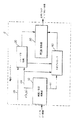
図2は、嗜好シャープナー2のブロック図を示す。ディジタルカラー画像と(ノイズテーブル6の形式の)ノイズ情報は、嗜好シャープナー2へ入力される。ノイズ情報は、輝度テーブルの形式で入力される。ディジタル画像は、輝度ディジタル画像チャネルn(x,y)と2つの色差ディジタル画像チャネルg(x,y)とi(x,y)を生成するために、輝度/色差変換器10に入力される。輝度ディジタル画像チャネルn(x,y)と輝度ノイズテーブルは、システムノイズの知識に基づきディジタル画像チャネルn(x,y)を改善するために、それぞれのライン11aと11bを介して、シャープ化プロセッサ20へ入力される。分離した赤、緑,青画像チャネルを含むRGB空間内のディジタルカラー画像から、輝度-色差カラー空間への変換器10内で行われる変換は、典型的には、カラー空間マトリクス変換により行われ、従来技術で既知な、輝度ディジタル画像チャネルn(x,y)と、2つの色差ディジタルチャネルg(x,y)とi(x,y)となる。好適な実施例では、輝度色差空間へのマトリクス変換は、以下の式により行われる。
【0018】
【数1】

【0019】
シャープ化プロセッサ20へのノイズテーブル入力は、信号強度レベルiとその強度レベルに対する予想するノイズσN(i)の量の間の関係を提供する。
好適な実施例では、更に詳細に説明するが、ノイズテーブルは2コラムテーブルであり、第1コラムは強度レベルiを示し第2コラムはその強度レベルに対する予想するノイズσn(i)の標準偏差を示す。
【0020】
色差ディジタル画像チャネルg(x,y)とi(x,y)は、ライン11cを介して色差プロセッサ40に入力され、そして、望むように調整される。例えば、色差プロセッサ40の動作は、明らかな飽和を増加するために、1.0よりも大きい一定値により色差画像チャネルを落とすことでも良い。色差プロセッサの動作は、本発明に得に関連はないので、本実施例において色差プロセッサ40の出力が入力と同一に維持されるということに注意することを除いては、以後説明しない。
【0021】
シャープ化プロセッサ20からのディジタル画像チャネル出力と色差プロセッサ40からのディジタル画像チャネル出力は、赤,緑,青ディジタル画像チャネルより構成されるディジタル画像へ逆に変換するために、RGB変換器30へ入力される。この変換は、再び、マトリクス回転(即ち、変換器10により成された前のカラー回転マトリクスの逆)で達成される。3x3マトリクスを反転することは従来技術で既知であり、これ以上説明しない。RGB変換器30の出力は操作者の嗜好に関してシャープ化されれたディジタル画像である。
【0022】
好適な実施例で説明したように、シャープ化プロセッサ20は輝度ディジタル画像チャネルのみに作用する。しかし、別の実施例では、シャープ化プロセッサは各赤,緑,青ディジタル画像チャネルに適用できる。この場合、ディジタルカラー画像信号(RGB信号)は直接シャープ化プロセッサ20へ与えられる。
【0023】
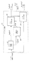
図3では、シャープ化プロセッサ20のブロック図を示し、ディジタル画像チャネルn(x,y)は、ペデスタル分割器50により2つの部分に即ち、ペデスタル信号とテクスチャ信号に分割される。図5に示すペデスタル分割器50の好適な実施例は、テクスチャ信号ntxt(x,y)とペデスタル信号nped(x,y)を出力する。テクスチャ信号ntxt(x,y)はおもに画像の細部と画像のノイズを含む。ペデスタル信号が遷移エッジを含む大きな閉塞境界を含む画像の領域を除いては、ペデスタル信号nped(x,y)は概念的にスムーズな信号である。図5Aに示すペデスタル分割器50の別の実施例は本質的に線形FIRフィルタを含む。この別の実施例では、ペデスタル信号nped(x,y)は、本質的に低域通過信号に等しくそして、テクスチャ信号ntxt(x,y)は本質的に高域通過信号である。空間周波数分割が可能なので、当業者は本発明は、テクスチャ信号とペデスタル信号のどのような定義に関しても有益な結果を生むことは理解されよう。
【0024】
再び図3を参照すると、ディジタル画像チャネルn(x,y)、テクスチャ信号ntxt(x,y)及び、ノイズテーブル6は、テクスチャ変更器70へ入力される。テクスチャ変更器70の目的は、ノイズに敏感な方法で、シーンの細部の大きさを高めることである。局部信号/ノイズ比(SNR)の推定は、ノイズテーブルにより供給される所定の強度レベルに関する予想されるノイズの標準偏差に関する情報を使用してなされる。この局部SNRの推定は、テクスチャ信号の局部レベルに与えられる改善及び、レベルに関連するブーストファクタを設定するのに使用される。以下に手順を詳細に示す。テクスチャ変更器70の出力は、改善されたテクスチャ信号n’txt(x,y)である。更に、ペデスタル信号nped(x,y)は、エッジが大きな明瞭さとシャープさを有するように見えるようにするエッジコントラストを増加するための、ペデスタル変更器60の入力である。ペデスタル変更器60の目的は、欠陥を生じずに、画像エッジを改善することである。ペデスタル変更器60により採用されている方法を以下に詳細に説明する。ペデスタル変更器の出力は、改善されたペデスタル信号n’ped(x,y)である。
【0025】
ペデスタル変更器60とテクスチャ変更器70の出力は、シャープ化プロセッサ20からのディジタル画像チャネル出力を生成するために、改善されたテクスチャ信号n’txt(x,y)と改善されたペデスタル信号n’ped(x,y)とを加算する加算器80に入力される。改善されたディジタル画像チャネルn’(x,y)は、
n’(x,y)=n’txt(x,y)+n’ped(x,y)
のように表される。
【0026】
図4は、シャープ化プロセッサ20の別の実施例を示し、構成要素の配置の僅かな摂動はしばしばシャープ化プロセッサ20の出力への僅かな効果のみを有することを示す。これに関し、ペデスタル分割器50は、テクスチャ信号ntxt(x,y)と回避信号a(x,y)を出力する。回避信号a(x,y)は画像のエッジの位置を決定するために、ペデスタル分割器50により計算された中間的な信号である。この信号の導出を、以下に説明する。回避信号の範囲は0.0から1.0の範囲である。回避信号の値a(x,y)=0.0を有する画像位置(x,y)は、画像のエッジ領域に対応し、逆に、回避信号の値a(x,y)>0.0を有する画像位置(x,y)は、画像の細部又はノイズの領域に対応する。前述のように、本発明の目的は、細部、大きなエッジ及び、ノイズのある領域に適用される改善の独立した制御を可能とすることである。従って、シャープ化プロセッサ20からのディジタル画像チャネル出力ないでは、エッジ(a(x,y)=0.0)がペデスタル変更器60により改善されそして、画像の細部又はノイズ(a(x,y)>0.0に対応する位置)の領域は、テクスチャ変更器70により改善されることが望ましい。
【0027】
このために、ディジタル画像チャネルn(x,y)は、ペデスタル変更器60に入力され、そして、前に、テクスチャ信号ntxt(x,y)がテクスチャ変更器70へ入力され得る。ペデスタル変更器60とテクスチャ変更器70からの2つの結果の出力、改善されたテクスチャ信号n’txt(x,y)及び、ペデスタル信号n’ped(x,y)は、回避加算器81へ入力される。回避加算器81は、3入力が必要である。2つの信号n’txt(x,y)とn’ped(x,y)が加算され、欠陥回避信号(a(x,y))である。加算される2つの信号は、加算されるべき1つの信号はa(x,y)により乗算され、そして、他の信号は(1−a(x,y))により乗算されるように変換を受ける。a(x,y)によりスケーリングされている信号入力は、回避加算器81の”a(x,y)入力”として知られ、そして、(1−a(x,y))によりスケーリングされている信号入力は、回避加算器81の” (1−a(x,y))入力”として知られる。シャープ化プロセッサ20の本発明の場合は、回避加算器からの信号出力は、
n’(x,y)=a(x,y)ntxt(x,y)+(1−a(x,y))nped(x,y)
と表現できる。
【0028】
図5を参照すると、ペデスタル分割器50へのディジタル画像チャネルn(x,y)入力は、周波数分割器94により、高域通過信号nhp(x,y)と低域通過信号nlp(x,y)に分割される。高域通過信号と低域通過信号を発生する多くの既知の技術があるが、周波数分割器は、標準偏差(シグマ)0.9画素を有するガウシャンフィルタで実行することが好ましい。ガウシャンフィルタの標準偏差の好ましい値は、画像サイズによって変わる。0.9画素の標準偏差の値は、本発明のを1024x1536画素サイズの画像に最適化することにより得られる。ガウシャンフィルタは、2次元循環対象低域通過フィルタで有り、フィルタ係数は従来技術で既知の以下の公式により得られる。
g(i,j)=1/(sigma sqrt(2π)exp[−(i2+j2)/(2sigma2)]
ここで、g(i,j)=(i,j)番目の画素のガウシャンフィルタ係数であり、
sigma=ガウシャンフィルタ(0.9)の標準偏差であり、
π=約3.1415...の定数である。
【0029】
好適な実施例では、フィルタg(i,j)については合計で49係数に関して、iとjは−3から+3の範囲(両端を含めて)である。他の技術、位置の技術では、ガウシャンフィルタを、計算コストの低減のために、続くアプリケーションに対して、水平及び垂直成分へ分割するものがある。いずれの場合にも、周波数分割器94は、ガウシャンフィルタg(i,j)を従来既知の畳み込み処理によりディジタル画像チャネルn(x,y)へ適用する。畳み込みは、
nlp(x,y)=ΣΣn(x−i,y−j)g(i,j)
により表される。ここで、合計は、全iとjに亘って起こる。この畳み込み処理からの信号nlp(x,y)は、低域通過信号である。低域通過信号は、周波数分割器94から出力される。更に、高域通過信号nhp(x,y)は、以下の関係、
nhp(x,y)=n(x,y)−nlp(x,y)
により得られた後に周波数分割器94から出力される。
【0030】
低域通過信号nlp(x,y)は、以下に詳細に説明するように、回避信号a(x,y)を形成するために、回避信号発生器104へ入力される。テクスチャ発生器90は、両高域通過信号nhp(x,y)と回避信号a(x,y)を受信しそして、両信号は、テクスチャ信号ntxt(x,y)を生成するために、そこで乗算される。従って、テクスチャ信号ntxt(x,y)は、
ntxt(x,y)=a(x,y)*nhp(x,y)
と表される。テクスチャ信号ntxt(x,y)は、テクスチャ発生器90により計算されそして、ペデスタル分割器50により出力される。更に、図5の破線で示すように、回避信号a(x,y)は、特に図4に示すシャープ化プロセッサ20の他の実施例の回避加算器81に入力を供給するために、随意にペデスタル分割器50から出力される。
【0031】
ペデスタル発生器100は、輝度ディジタル画像チャネルn(x,y)とテクスチャ信号ntxt(x,y)を受信し、輝度信号からテクスチャ信号を減算し、ペデスタル信号nped(x,y)を生成する。このペデスタル信号は、
nped(x,y)=n(x,y)−ntxt(x,y)
で表される。ペデスタル発生器100により計算されたペデスタル信号nped(x,y)は、ペデスタル分割器50から出力される。
【0032】
(50Aとして識別される)ペデスタル分割器50の代わりの実施例を、図5に示す。ペデスタル分割器50Aの代わりの実施例に入力された輝度ディジタル画像チャネルn(x,y)は、0.9画素の標準偏差(シグマ)を有する上述のガウシャンフィルタが好ましい周波数分割器94により高域通過信号と低域通過信号に分けられる。ガウシャンフィルタの標準偏差の好適な値は、画像サイズにより変わる。0.9画素の標準偏差の値は1024x1536画素サイズの画像を本発明に最適化することにより得られた。周波数分割器94は、上述の畳み込み処理により、ガウシャンフィルタg(i,j)にディジタル画像チャネルn(x,y)を与える。
【0033】
この畳み込み処理からの信号nlp(x,y)は周波数分割器94から出力された低域通過信号である。更に、高域通過信号nh p(x,y)も、以下の関係、
nhp(x,y)=n(x,y)−nlp(x,y)
により得られた後に、周波数分割器94から出力される。
【0034】
ペデスタル分割器のこの代わりの実施例では、低域通過信号nlp(x,y)はペデスタル分割器から、ペデスタル信号nped(x,y)として出力される。(即ちこの場合には、ペデスタル信号nped(x,y)は、制御信号と共に得られるよりも、低域通過信号nlp(x,y)に等しいと設定される。同様にテクスチャ信号ntxt(x,y)も高域通過信号nhp(x,y)に等しいと設定される。
【0035】
ペデスタル分割器50Aのこの代わりの実施例は、単に畳み込みによりディジタルフィルタ動作を行い、そして、テクスチャ信号とペデスタル信号として、高域通過信号と低域通過信号をそれぞれ出力する。ペデスタル分割器50Aのこの実施例は、制御信号は使用されず又は計算されないので、好適な実施例50よりも単純である。しかし、この代わりの実施例を採用する嗜好シャープナー4からのディジタル画像信号の品質は、ペデスタル分割器50の好適な実施例を採用する嗜好シャープナー4からのディジタル画像信号の品質よりも悪い。
【0036】
当業者は、本質的に合計してディジタル信号を発生する2つの信号を発生するのに使用され得る多くの形式の動作があることがわかる。ペデスタル分割器の好適な実施例とペデスタル分割器の代わりの実施例は、両方ともに、本質的に合計してディジタル信号を発生する2つの信号にディジタル画像チャネルを分割するのに使用され得る、動作の例である。
【0037】
図6は、回避信号発生器104のブロック図を示す。これに関し、低域通過信号nlp(x,y)は、非方向グラディエント信号を発生する非方向2乗グラディエント計算器106へ入力される。この計算は最初に画素とその上方の垂直隣接画素間の差を計算し、画素とその右方の水平隣接画素間の差を計算することにより行われる。非方向2乗グラディエントは、これらの2つの差の2乗和である。非方向2乗グラディエントndg(x,y)は以下の式、
ndg(x,y)=[nlp(x,y)−nlp(x−1,y)]2+[nlp(x,y)−nlp(x,y+1)]2
で表される。回避信号発生器104の出力から欠陥回避信号a(x,y)を生成するために、ndg(x,y)の値は、欠陥回避機能アプリケータ108によりマップされる。
【0038】
図6を参照し、このマッピングは、以下のように形成された欠陥回避関数av(y)を通して、非方向グラディエント信号ndg(x,y)を渡すことにより行われる。本発明の好適な実施例は、以下により定義される欠陥回避関数を使用する。
y>C0且つy<C1に対して、
av(y)=(1/2)(1+COS(π(y−C0)/(C1−C0))、
y>=C1に対して、av(y)=0、
y<=C0に対してav(y)=1であり、ここで、C0とC1は、定数値である。
【0039】
C0とC1の好適な値は、入力データの範囲により変わる。本好適な実施例の展開で使用される画像内の入力データ範囲は0から4095である。この場合、C0の好適な値は996であり、C1の好適な値は8400である。欠陥回避関数を構成する代わりの方法は、以下の式により表される。
y>=C0且つy<=C1に対して、
av(y)=1−sqrt((y−C0)/(C1−C0))
y<C0に対して、av(y)=1、
y>C1に対してav(y)=0である。図7は関数av(y)のプロットを示す。
【0040】
好適な実施例では、C1の値は、ガウシャンフィルタの(標準偏差の)サイズシグマに関連する。C1の値は、ガウシャンフィルタの(標準偏差の)シグマの2乗に反非例する。好ましくは、C1は、
C1=6804/(sigma*sigma)
の関係により決定され得る。
また、C0はC1に、
C0=0.127C1−18
により関連する。
【0041】
欠陥回避信号a(x,y)は、欠陥回避機能アプリケータ108により発生される。これは、図7に示すように、非方向2乗グラディエントndg(x,y)へ、欠陥回避関数a(x,y)を与えることにより達成される。数学的な結果は、
a(x,y)=av(ndg(x,y))
式により与えられる。図7に示す欠陥回避信号は、ルックアップテーブル(LUT)として最も効率良く実行される。
【0042】
回避信号a(x,y)はディジタル画像チャネルの空間的にフィルタされたものから形成される制御信号の例であるということを理解するのに役立つ。先ず最初に、一般化された線形空間フィルタは、式
c(x,y)=ΣΣd(x−i,y−i)g(i,j)
により与えられる。ここで、d(x,y)値は(x,y)番目の画素の周りの局部画素値を表し、g(i,j)は、画素値に依存しないディジタルフィルタの数値係数を示す。ここで記述される非線形空間フィルタは、sン系空間フィルタ式により表せない空間フィルタとして定義されるべきである。一般化された制御信号を入力信号に与える出力は、入力信号と乗算的関係にある。制御信号は式、
c(x,y)=h(x,y)d(x,y)
により与えられる。ここでd(x,y)値は、入力信号(x,y)番目の画素値を表し、h(x,y)値は制御信号の(x,y)番目の画素値を表す。制御信号を入力信号に与える結果は、制御信号が入力信号の空間フィルタされたものから得られるならば、非線形空間フィルタの一般的なカテゴリーに入る。回避信号a(x,y)はディジタル画像チャネルの空間的にフィルタされたものから形成された制御信号の例である。好適な実施例で記述されたテクスチャ信号ntxt(x,y)は、制御信号の適用と画像チャネルn(x,y)へ与えられたディジタルフィルタで生成された非線形空間フィルタの例である。
【0043】
図8を参照すると、そこに示されているペデスタル変更器60は、(2次元ウインドウにより分離された)ディジタル画像チャネルの局部化された領域に亘って計算された1つ又はそれ以上の画像特性に基づく、ディジタル画像チャネルの形態に適用できるシャープ化フィルタアルゴリズムである。フィルタアルゴリズムは、ディジタル画像チャネルの局部化された領域に亘って画像特性に関するスケーリング関数でトーンスケールを正規化しそして、ディジタル画像チャネル内のエッジの構造を再整形するためにスケーリングされたトーンスケールを使用する段階を含む。特に、局部トーンスケール関数の形は、画層処理前に元々選択されているが、しかし、局部トーンスケール動作の正確なスケーリングと変換は、局部化された領域の統計により決定される。従って、領域が分離された後は、アルゴリズムの実行は、局部領域から所望の統計的性質を識別し、統計的性質に関連して正規化された局部トーンスケール変換を行い、そして、トーンスケール変換を通して、改善された中央画素値を発生するために局部領域の中央画素をマッピングすることを含む。ペデスタル変更器60の更なる詳細は、1999年7月2日にA.G.GallagherとE.B.Gindeleにより出願された、発明の名称”ディジタル画像のエッジコントラストを改善する方法(A Method for Enhancing the Edge Contrastof a Digital Image)”の米国特許出願番号09/324,239に開示されており、参照によりここに組み込まれる。
【0044】
ペデスタル変更器60は幾つかのモードで実行され得る。特に図8に示すブロック図では、ペデスタル変更器60は、第1のモードでは、入力画素値を各領域の極大値及び極小値にスケーリングし、そして、スケーリングされた入力値を正規化された座標でトーンスケール関数へ与えることにより行われる。変換動作により得られた出力は、改善された出力値を得るために、(入力を発生するのに使用された)スケーリング関数の逆関数で処理される。代わりに、ペデスタル変更器60を実行する第2のモードでは、局部トーンスケールは、各領域の極大値と極小値に結びついている座標で構成され、そして、各中央値はトーンスケール関数の結び付けられている座標を通してマップされる。これは、改善された出力値を直接生成する。第3のモードでは、トーンスケール関数の入力のみが逆スケーリング関数でスケーリングされ、そして、出芽疎は逆スケーリング関数で処理される。第4のモードでは、トーンスケール関数の出力のみがスケーリングされ、そして、入力画素はスケーリング関数で処理される。どのモードでも、トーンスケール関数の形は画像に亘って固定されたままであるが、しかし、領域の統計的性質に従ってトーンスケール関数の形を変えることが望ましい。さらに、正規化されたトーンスケール動作を実質的に入力ディジタル画像チャネルの全画素に適用するのが典型的であろうが、ディジタル画像チャネルの選択された領域にこの方法を適用するのが望ましい。第2、第3及び、第4のモードの詳細に関しては、前述の出願番号09/324,239に向けられており、参照によりここに組み込まれる。これらの代わりのモードは好適な実施例(即ち、図8の第1モード)で開示されたペデスタル変更器60により得られる処理されたディジタル画像チャネルと同一の処理されたディジタル画像チャネルを提供する。
【0045】
更に図8は、上述の第1モードに従った60を実行するための好適な実施例のブロック図を示す。ペデスタル変更器60の好適な実施例は、例えば、寸法が高さが1024画素で、幅が1536画素の比較的高い解像度のディジタル画像チャネルを参照して説明されるが、本発明のそれ以上の又はそれ以下の解像度を有する画像チャネルで同様に動作可能である。しかし、画像解像度の選択は、ウインドウサイズに付随する効果を有する。即ち、5x5ウインドウは1024x1536解像度に好ましいことがわかるが、より高い解像度の画像センサは通常は大きなウインドウサイズを可能とし、そして、低解像度センサは逆である。
【0046】
図9を参照すると、ディジタル画像チャネルのディジタル表現の各入力中央画素110の値は、最初に、局部統計を計算する局部統計決定器116へ送られる。局部領域112内に含まれる周辺画素114の値も、局部統計決定器116へ送られる。局部領域112と入力画素110は、ディジタル画像チャネルの空間領域を構成する。好適な実施例では、各入力画素110についての局部領域は、入力画素が中心の、局部統計が決定される隣接矩形領域として定義される。好適な実施例では、局部領域は各サイドが5画素の矩形隣接部である。図9は、好適な実施例で実行される局部領域を示す。局部領域112内に含まれる画素114は、局部統計決定器116へ渡される入力画素110を囲む(斜線で示す)24画素として示される。当業者は、本発明は、大きな種々の局部領域サイズと形で動作することが理解されよう。そして、(本記述及び、請求項で)処理された画素を記述するための用語”中央”の使用は、その局部領域の重心での画素よりも画素の局部的な周囲を有する画素を単に参照する。
【0047】
図8は、各中央画素110の値uは、局部統計決定器116とスケーリング関数評価器120へ入力される。更に、局部領域内の画素114の値は、局部領域の統計的性質を発生するために局部統計決定器116へ入力される。スケーリング関数発生器118は、各入力画素110の値uを正規化するためにスケーリング関数評価器120へ与えられるスケーリング関数s(x)を発生するために統計的性質を使用し、それにより、第1の中間値Iを発生する。統計的性質は、スケーリング関数s(x)の逆である関数s−1(x)を発生するための逆スケーリング関数評価器122によっても使用される。第1の中間値Iは、中間値Iをトーンスケール関数f(x)を通してマップする、第2の中間値I2を発生するためのトーンスケール発生器126により提供されるトーンスケールアプリケータ124へ与えられる。トーンスケールアプリケータ124からの出力中間値I2は、逆スケーリング関数アプリケータ128へ与えられ、逆スケーリング関数発生器122により提供される逆関数s−1(x)を使用してシステム画像空間内で処理された値u’を発生する。
【0048】
特に、局部統計決定器116は局部領域112と入力画素110内に含まれる画像データを記述する幾つかの特性を計算する。局部統計は、局部領域112と入力画素110に含まれる画素値の数学的な結合であろう。好適な実施例では、局部統計決定器116は、2つの局部統計、局部領域112と入力画素110からの最大及び、最小画素値を決定する。代わりに、局部統計決定器116は、n最大画素値の平均とm最小画素値の平均を決定する。ここで、nとmは局部領域112に含まれる画素数よりも非常に小さい整数であり、例えば、n=m=3である。前述のように、これらの局部統計はスケーリング関数s(x)と逆スケーリング関数s−1(x)の発生で使用される。
【0049】
局部統計決定器116で決定される局部統計は、スケーリング関数発生器118と逆スケーリング関数発生器122へ送られる。好適な実施例では、スケーリング関数は以下の式、
【0050】
【数2】
【0051】
同様な方法で、逆スケーリング関数発生器122は、逆スケーリング関数s−1(u)を形成する。逆スケーリング関数s−1(u)は、以下の式、
s−1(u)=u(X−N)+N
で表される。逆スケーリング関数の目的は、トーンスケール関数130から得られた出力値を期間[N X]へ戻すために、スケーリングすることである。スケーリング関数と逆スケーリング関数は逆であり、s−1(s(u))=uと簡単に示すことができる。
【0052】
入力画素110の値は、中間値I=s(u)を発生するために、スケーリング関数評価器120へ送られる。ここで、Iは中間値であり、s(x)はスケーリング関数であり、uは入力画素110の値である。スケーリング関数評価器120の出力は、中間値Iである。中間値Iは、トーンスケールアプリケータ124へ送られる。トーンスケールアプリケータ124の目的は、局部領域112に関して入力画素110の値のコントラストに影響を与えることである。トーンスケールアプリケータ124、中間値Iを変更し、それにより、第2の中間値I2を形成する。トーンスケールアプリケータ124は、中間値Iをトーンスケール関数130で(即ち、f(x)で)変更する。このように、トーンスケールアプリケータの動作は以下の式I2=f(I)で表される。ここでI2は、第2の中間値、f(x)はトーンスケール関数、そしてIはスケーリング関数評価器120からの出力である。
【0053】
トーンスケール関数f(x)は、トーンスケール発生器126により発生される。好適な実施例では、トーンスケール関数f(x)は、S字状の関数であり、ガウス確率分布関数を積分することにより形成され、そして、従来技術では既知である。S字状関数は完全に、積分されるガウス確率分布関数の標準偏差σにより特徴化される。トーンスケール関数f(x)は、以下の式、
【0054】
【数3】
【0055】
【数4】
【0056】
x=0.5で評価されるトーンスケール関数f(x)の傾斜は、関係、
【0057】
【数5】
【0058】
図10は、種々のスケール関数を示し、1つはトーンスケール関数130として示され、そして、関連するガウス確率関数の標準偏差はσである。当業者には、S字状関数に加えて、広く種々の関数がトーンスケールアプリケータ124の目的を達すると認めるであろう。
【0059】
トーンスケールアプリケータ124から出力された第2の中間値I2は、逆スケーリング関数アプリケータ128へ送られる。加えて、逆スケーリング関数発生器122から出力された逆スケーリング関数s−1(x)は、逆スケーリング関数アプリケータ128送られる。逆スケーリング関数アプリケータ128の目的は、第2の中間値I2からの処理された画素値u’を発生することである。逆スケーリング関数アプリケータ128は、逆スケーリング関数
u’=s−1(I2)
を評価することにより、改善された画素値u’を発生する。
I2とIを置きかえると、
u’=s−1(f{s(u)})
となる。ここで、s−1は逆スケーリング関数を示し、f{x}はトーンスケール関数を示し、s(x)はスケーリング関数を示し、uは入力画素110の値を示し、u’は改善された画素の値を示す。ペデスタル変更器60から出力されたディジタル画像チャネルは、改善されたペデスタル信号n’ped(x,y)である。
【0060】
典型的には、ペデスタル変更器60からの処理された画素値u’を発生する処理は、ディジタル画像チャネル内の各画素に対応する処理された画素値を発生するために、ディジタル画像チャネル内の各画素に繰り返される。これらの処理された画素値は、集合として考えられるときには、処理されたディジタル画像チャネルを構成する。代わりに、処理された画素値u’を発生する処理は、ディジタル画像チャネル内の各画素のサブセットに対応する処理された画素値を発生するために、ディジタル画像チャネル内の各画素のサブセットに繰り返される。後者の場合は、集合として考えられるときには、サブセットは、チャネルの一部の処理された画像を構成する。一般的には、本アルゴリズムのパラメータは、高いエッジコントラストの出現とディジタル画像チャネルよりも更に明瞭な改善されたディジタル画像チャネルを生成するために調整され得る。
【0061】
ペデスタル変更器60は、(シャープ化フィルタのウインドウサイズにより記述され得る)局部領域のサイズと、(トーンスケール関数の傾斜により記述され得る)トーンスケール変換関数の形の2つのパラメータを定義する。アルゴリズムは、例えば、1024x1536画像器に対しては、約7X7画素よりも大きくないウインドウサイズかかなり小さい場合には、最も良く動作する傾向にある。確かに、局部トーンスケール関数のウインドウサイズと傾斜が上昇するにつれて、画像は”ペイントバイナンバー”欠陥を有し始める。また、大きなウインドウは、画像内の大きな閉鎖境界形式エッジのいずれの側でもテクスチャを含む傾向にある。この効果は、ウインドウサイズを比較的小さく維持することにより減少される。5X5又は、それ以下の画素のウインドウは、一般的には、1024X1536解像度の典型的な状況で満足な結果を生じるために好ましいことがわかる。前述のように、他の好適なウインドウサイズは他の画像解像度に対する困難性なしに、経験的に決定され得る。代わりに、大きなウインドウのシャープ化効果を得るために欠陥が増加しても良い場合には、大きなウインドウは所定の解像度の特定の状況で受け入れ可能である。
【0062】
ここで記述したペデスタル変更器は領域の統計的性質に従って、例えば、中央画素が実質的に極大値と極小値の中間にある場合を除いて、中央値を極大値又は極小値に向かって駆動することにより、中央画素の値を制御する優位点を有する。従って、エッジ遷移は画像入力よりも、画素の狭い範囲で発生し、これにより、元の画像よりもシャープで更に焦点の合ったように見える画像を発生する。更に、トーンスケール変換の出力は、例えば、領域の極大値及び極小値により結び付けられる統計的性質により変更されているので、エッジ境界でのシステム的なオーバーシュート及びアンダーシュートは、消滅し、且つリンギング欠陥も知覚できない。
【0063】
図11は本発明に従ったテクスチャ変更器70の詳細を示す。テクスチャ変更器70は、ディジタル画像チャネルn(x,y)、テクスチャ信号ntxt(x,y)及び、輝度ノイズテーブル6を入力する。テクスチャ変更器70の出力は、テクスチャ信号n’txt(x,y)により改善される。テクスチャ変更器70の目的は、局部信号対雑音比(SNR)の推定値に関連するファクタによりテクスチャ信号をブーストすることである。このように、高SNRを有するディジタル画像チャネルの領域と一致するテクスチャ信号の部分は、ディジタル画像チャネルの低SNR領域に関連するテクスチャ信号の部分と比較して、大きなブーストレベルであることを経験する。例えば、シャープ化される画像がきれいな青空の大きな領域を含んでいるとする。この領域の唯一の変調は画像化システムからのノイズであるようである。従って、この変調の振幅を増加するのは好ましくない。一方、草原の変調は画像システムノイズに加えて、多くの草の葉による変調の結果である。この場合には、シーンの実際の変調に属するので、変調をブーストするのが好ましい。本発明では、信号対雑音比は、例えば、シーンの2つの前述の形式の領域間を区別するのに使用され得る分類器として働くと推定される。
【0064】
これに関しては、ディジタル画像チャネルn(x,y)、テクスチャ信号ntxt(x,y)及び、輝度ノイズテーブル6は、局部SNR推定器160へ入力される。局部SNR推定器160の目的は、テクスチャ信号の特定の画素に与えられるブーストのレベルを決定するのに後に使用される局部信号対ノイズ比を推定することである。好適な実施例では、局部SNR推定器160の出力は、シンボルSNR(x,y)で表される、ディジタル画像チャネル内の各画素に対するSNRの1つの推定値である。しかし、SNRは、ディジタル画像チャネルの画素の位置のサブセットのみに対して計算されることも可能である。局部SNR推定器160を以下に詳細に説明する。
【0065】
局部SNR推定器160の出力、SNR(x,y)は、ゲイン決定器134に送られる。ゲイン決定器134は、局部SNRの推定値が既知の場合には、テクスチャ信号の各々の特定の(x,y)位置で与えるブーストB(x,y)のここのレベルを決定することを意味する。これは、例えば、図15に示す、ルックアップテーブル(LUT)により達成される。好適な実施例では、LUTは単調に増加する。LUT出力(ゲイン)はLUT入力(SNRの推定値)の増加と共に増加する。
【0066】
図15に示すLUTに関する式は、
SNR(x,y)<SNRminの場合には、B(x,y)=sfmin、
SNRmin<SNR(x,y)<SNRmaxの場合には、
B(x,y)=sfmin+(sfmax−sfmin)(SNR(x,y)−SNRmin)/(SNRmax(x,y)−SNRmin)、
SNR(x,y)>SNRmaxの場合には、B(x,y)=sfmaxである。
ここで、sfmax>sfminであり、且つSNRmax≧SNRminである。好適な実施例では、sfmaxは3.5であり、sfminは2.0であり、SNRmaxは2.0であり、SNRminは0.4である。
【0067】
ゲイン決定器134により出力されるゲインB(x,y)とテクスチャ信号ntxt(x,y)はともに、テクスチャブースタ136へ送られる。テクスチャブースタ136の目的は、関連するゲインでテクスチャ信号ntxt(x,y)の各値を乗算することである。テクスチャブースタ136の出力は、改善されたテクスチャ信号n’txt(x,y)であり、式
n’txt(x,y)=ntxt(x,y)*B(x,y)
により与えられる。テクスチャ変更器70から出力されるこの改善されたテクスチャ信号n’txt(x,y)は、図3の加算器80へ(又は、図4に示す代わりの実施例の場合には回避加算器81)送られる。B(x,y)<1.0の時には、改善された信号の大きさは、元のテクスチャ信号の大きさより小さい、
|ntxt(x,y)|>|n’txt(x,y)|ことに注意する。このように本発明は、ノイズの多い領域、B(x,y)<1.0で、処理されたディジタル画像は嗜好シャープナー2に入力されたディジタル画像チャネルよりもノイズが少ない。
【0068】
局部SNR推定器160の詳細なブロック図を図12に示す。ディジタル画像チャネルn(x,y)は、最初に局部分散コンピュータ170に入力される。局部分散コンピュータ170の目的は、信号の活動の局部推定値を得ることである。好適な実施例では、局部分散コンピュータ170はサイズWxW画素のウインドウに亘って局部分散σR 2(x,y)を計算する。好適な実施例では、W=7画素であるが、代わりのサイズのウインドウも等価な結果でタスクを実行することが決定された。
【0069】
値の組の局部分散の計算は従来技術で既知であり、
【0070】
【数6】
【0071】
減算器172はディジタル画像チャネル(x,y)と、テクスチャ信号ntx t(x,y)の両方を入力する。減算器172はペデスタル信号nped(x,y)である。減算器172は、以下の公式に従って、
nped(x,y)=n(x,y)−ntxt(x,y)
ディジタル画像チャネル(x,y)からテクスチャ信号ntxt(x,y)を減算する。このペデスタル信号nped(x,y)は、ペデスタル分割器50により決定されるペデスタル信号と同一である。本発明の実際の実行では、ペデスタル信号は、1回のみ計算されることを要する。
【0072】
ノイズテーブル6とペデスタル信号nped(x,y)は、予想されるノイズ決定器190に入力される。ノイズテーブルは、予想されるノイズとσN(i)とディジタル画像チャネル(x,y)の強度iの間の関係を含む。好適な実施例では、ノイズテーブルは2つのコラムのテーブルであり、2コラムリストのそのサンプルを以下に示す。最初のコラムは強度レベルを示し、第2のコラムはその強度レベルに対するノイズの予想される標準偏差を示す。
【0073】
【表1】
【0074】
【数7】
【0075】
【数8】
【0076】
予想されるノイズ決定器190は、ペデスタル信号nped(x,y)の強度レベルに関するノイズσN(x,y)の標準偏差の強度に依存する推定値を出力する。予想されるノイズ決定器190は、ペデスタル信号の強度をノイズσN(x,y)の予想される標準偏差に関連させるテーブルルックアップを行うか、又は、上述のように予想されるノイズを計算する。予想されるノイズ決定器190の出力σN(x,y)は、
σN(x,y)=σN(nped(x,y))
と表される。値nped(x,y)がσn(i)の存在する値iと一致する場合には、線形補間がσn(nped(x,y))を決定するのに使用される。線形補間は既知であるので更に説明しない。図14はノイズテーブルのプロットを示す。
【0077】
図14に示すようなノイズテーブルを発生する手順は、Gray他による1997年6月24日に発行された米国特許番号5,641,596又は、Snyder他による1999年7月13日に発行された米国特許番号5,923,775により開示されており、両者ともに参照により組み込まれる。
【0078】
SNR計算器180は予想されるノイズ決定器190から出力されたノイズσN(x,y)の予想される標準偏差と、局部分散コンピュータ170から出力された局部分散σR 2(x,y)の両方を入力する。SNR計算器180は、信号分散の比を計算することにより、局部信号対雑音比SNR(x,y)を推定する(局部分散σR 2(x,y)は信号による分散とノイズによる分散の和{RMSの意味}である)。このように、SNR計算器180の出力は、以下の公式
【0079】
【数9】
【0080】
信号対雑音比の多くの他の推定値が本発明の範囲を超えることなく公式化されうることに注意する。例えば、図13は局部SNR推定器160の代わりの実施例を示す。この実施例の目的は、図12に示すように計算的に更に安価に局部SNRの推定値を提供することである。この代わりの実施例では、ノイズと信号偏差は共にガウス分布とみなされ、標準偏差よりも平均絶対値偏差(MAD)の使用を可能とする。平均絶対値偏差の計算は、計算的に高価な平方根と2乗動作を含まない。この実施例では、テクスチャ信号ntxt(x,y)とディジタル画像チャネルn(x,y)は再び、前述のようにペデスタル信号nped(x,y)を生成するために、減算器172へ入力される。ペデスタル信号nped(x,y)は、再び値σN(x,y)を決定するために予想されるノイズ決定器190への入力として使用される。
【0081】
テクスチャ信号ntxt(x,y)はテクスチャ信号内の局部平均絶対値偏差を決定するために、局部MAD計算器200に入力される。テクスチャ信号ntxt(x,y)の平均値が0であるとすることにより、局部MAD計算器200により使用される局部MAD計算のための公式は、
MADR(x,y)=Σ|ntxt(x+i,y+j))|/W2
が使用される。ここで、平均絶対値偏差の計算に含まれる全W2=49画素について、iとjはともに−3から+3であることが好ましい。局部MAD計算器200は、平均絶対値偏差MADR(x,y)を出力する。これは後に局部SNRの推定値を決定するのに必要な計算に使用される。
【0082】
ノイズテーブル調整器210の目的は、テクスチャ信号のMADR(x,y)の計算と、ディジタル画像チャネルの標準偏差σR(x,y)の計算の間の差を保証することである。ノイズテーブル調整器210は、標準偏差よりも平均絶対値偏差を使用する目的で輝度ノイズテーブルを変更する。前述のように輝度ノイズテーブルは、予想されるノイズσn(i)と強度iの間の関係を含む。ガウス分布は以下の関係、
MAD=sqrt(2/π)σ
により分布の標準偏差σに関連することは既知である。輝度ノイズテーブルを標準偏差のメトリックから、MADのメトリックへ変換するために、各値σn(i)は、約0.8にスケーリングされねばならない。
【0083】
更に、この代わりの実施例と、信号が局部信号活動の測定値の計算に使用される好適な実施例の間に差がある。好適な実施例では、ディジタル画像チャネルの分散は計算される。この代わりの実施例では、テクスチャ信号が、MADR(x,y)の値を計算するのに使用され、信号平均がゼロと仮定される場合に計算的な利益を与える。テクスチャ信号ntxt(x,y)とディジタル画像チャネルn(x,y)の間の関係は、このために考慮する輝度ノイズテーブルを調整するために理解されねばならない。この関係は、テクスチャ信号を発生するのに使用されるディジタルフィルタ処理が線形であるときにのみは、簡単に表現される。このステップのために、欠陥回避信号の効果は無視され、テクスチャ信号は高域通過信号と等価であるとみなされる。i=−(n−1)/2、−(n−3)/2,...,n−1/2とj=−(m−1)/2、−(m−3)/2,...,m−1/2である係数h(i,j)の一般的なフィルタ(n x m)に関しては、フィルタされた信号の分散は以下の関係
σ2 fs=σ2 osΣΣh2(i,j)
による原信号の分散に関連する。ここで、σ2 fsはフィルタ信号の分散を示し、σ2 osは原信号の分散を示し、そして、合計はiとjに亘って起こる。
【0084】
本発明の場合には、フィルタh(i,j)は、
h(i,j)=δ(i,j)−g(i,j)
と表されるとする。ここで、δ(i,j)は、デルタ関数であり、i=0とj=0で1の値を有し、他ではゼロである。この式は、ガウシャンフィルタg(i,j)でディジタル画像チャネルを不鮮明にしそして、ディジタル画像チャネルから結果を減算する、ことにより(欠陥回避信号を無視して)テクスチャ信号を発生する前述の処理を説明する。このように、この記述を考慮することにより、ノイズテーブル調整器210は、ディジタル画像チャネルよりもテクスチャ信号上の局部信号活動の推定値を考慮するために、ファクタにより輝度ノイズテーブルの各値をスケーリングしなければならない。このファクタfは、
f=sqrt(ΣΣh(i,j)2)
であり、ここで、合計はiとjに亘って行われ、h(i,j)は前述している。輝度ノイズテーブルが標準偏差のユニット内であるので、分散よりも結果の平方根がとられる。
【0085】
このように、標準偏差よりもMADの計算をそして、ディジタル画像チャネルうよりもテクスチャ信号の計算補償する為に、ノイズテーブル調整器210の動作は、
m=f*sqrt(2/π)
に等しいファクタmによる輝度ノイズテーブルの各エントリσn(i)をスケーリングすることである。
【0086】
ノイズテーブル調整器210から出力される変更されたノイズテーブルは、ノイズMADN(x,y)からの予想されるMADの推定値を得る目的で、予想されるノイズ決定器190へ入力として送られる。予想されるノイズ決定器190は、各値nped(x,y)に対して、値MADN(x,y)を決定するためにノイズテーブルを使用する。予想されるノイズ決定器190の出力は、ディジタル画像チャネルの各位置での値MADN(x,y)である。
【0087】
図13に示す代わりの実施例のSNR計算器180は本質的に、好適な実施例のSNR計算器180と同じように動作する。SNR計算器180の目的はディジタル画像チャネルの各位置で推定されたSNRの値を出力することである。このために、SNR計算器180は以下の公式、
【0088】
【数10】
【0089】
【発明の効果】
要約すると、画像詳細を含む信号と主に大きな画像のエッジを含む他の信号へ画像を分割するペデスタル分割器50の使用により、エッジとテクスチャに与えられる改善の独立した制御を可能とする。エッジは、エッジコントラストを増加し境界の欠陥を避けるために、形態的動作により再整形される。テクスチャは、局部信号対雑音比の推定値に関して改善される。
【0090】
本発明を、好適な実施例を参照して説明した。本発明の範囲を超えること無く好適な実施例を変更できる。例えば、好適な実施例では、SNRの計算はディジタル画像チャネルの各画素に対して行われる。しかし、SNRの計算は計算コストを削減するために各N画素おきにのみ行われることも考えられ、そして、複製され、又は、補間される。SNRの計算は、ディジタル画像チャネルn(x,y)の局部分散計算を参照して説明した。更に、代わりの実施例では、記述された方法によりテクスチャ信号ntxt(x,y)に依るMADの計算の使用に基づき、局部SNRが推定される。当業者には、局部SNRはテクスチャ信号の分散の計算を実行することにより又は、ディジタル画像チャネルn(x,y)のMAD計算を実行することにより推定もされることは認識される。好適な実施例のそのような変更は、本発明の範囲から逸脱しない。
【図面の簡単な説明】
【図1】本発明の概略のブロック図である。
【図2】図1の選択シャープナーの詳細を示す図である。
【図3】図2に示すシャープ化処理器の第1の実施例のブロック図を示す図である。
【図4】図2に示すシャープ化処理器の第2の実施例のブロック図を示す図である。
【図5】図3に示すペデスタル分割器の第1の実施例のブロック図を示す図である。
【図5A】図3に示すペデスタル分割器の第2の実施例のブロック図を示す図である。
【図6】図5に示す回避信号発生器のブロック図を示す図である。
【図7】図6に示す回避信号発生器により与えられる欠陥回避機能の例を示す図である。
【図8】図3に示すペデスタル変更器のブロック図である。
【図9】画像の中央画素と関連する局部領域を示す画像の部分の例を示す図である。
【図10】幾つかのトーンスケール関数の例を示す図である。
【図11】図3に示すテクスチャ変更器のブロック図を示す図である。
【図12】図11に示す局部SNR推定器の第1の実施例のブロック図である。
【図13】図11に示す局部SNR推定器の第2の実施例のブロック図である。
【図14】ノイズテーブルを発生するのに使用される関数のプロットを示す図である。
【図15】図11に示すゲイン決定器により使用されるルックアップテーブル(LUT)のプロットを示す図である。
【符号の説明】
2 嗜好シャープナー
6 ノイズテーブル
10 輝度/色差変換器
11a 輝度ライン
11b ノイズテーブルライン
11c 色差テーブルライン
20 シャープ化プロセッサ
30 RGB変換器
40 色差プロセッサ
50 ペデスタル分割器
50A 代わりのペデスタル分割器
60 ペデスタル変更器
70 テクスチャ変更器
80 加算器
81 回避加算器
90 テクスチャ発生器
94 周波数分割器
100 ペデスタル発生器
104 回避信号発生器
106 非方向2乗グラディエント計算器
108 欠陥回避機能アプリケータ
110 入力中央画素
112 局部領域
114 周辺画素
116 局部統計決定器
118 スケーリング関数発生器
120 スケーリング関数評価器
122 逆スケーリング関数発生器
124 トーンスケールアプリケータ
126 トーンスケール発生器
128 逆スケーリング関数アプリケータ
130 トーンスケール関数
134 ゲイン決定器
136 テクスチャブースタ
160 局部SNR推定器
170 局部分散コンピュータ
172 減算器
180 SNR計算器
190 予想されるノイズ決定器
200 局部MAD計算器
210 ノイズテーブル調整器[0001]
BACKGROUND OF THE INVENTION
The present invention relates generally to digital image processing, and more particularly to a method for improving the edge contrast and texture of a digital image.
[0002]
[Prior art]
Conventional methods for improving the apparent sharpness of a digital image, such as unsharp masking techniques, often result in unwanted defects at large transition edges of the image. For example, unsharp masking is often
Sproc = Sorg + B (Sorg-Sus)
Is described by Where Sproc is the processed image signal with the high frequency components amplified, Sorg is the original image signal, Sus is the unsharp image signal, typically obtained by filtering the original image. And B is a high frequency enhancement signal.
[0003]
The unsharp masking operation is modeled as a linear system. Thus, the magnitude of any frequency in Sproc depends directly on the magnitude of that frequency in the Sorg image signal. As a result of this superposition principle, large edges in the Sorg image signal display ringing defects in the Sproc signal when the desired level of high frequency improvement is made in other areas of the Sproc signal. This ringing defect appears as a bright or dark outline around a large edge and is visually unpleasant.
[0004]
Many non-linear filters based on local statistics exist for noise reduction, sharpening and contrast adjustment. For example, median filters are known in the art. This filter typically provides noise reduction and each pixel is replaced with an intermediate value of several surrounding neighbors. This filtering is generally very beneficial in removing impulse noise, but the processed image is slightly less sharp than the original image.
[0005]
Another example of a non-linear filter based on local statistics is local histogram equalization, “Digital Image Processing, Second Edition” by William Pratt, John Wiley & Sons, 1991, pages 278-284, with adaptive histogram modifications and Has been referenced. With this filter, the pixel value is changed by the accumulated histogram of the local window. This technique effectively adjusts the contrast of each region of the digital image, effectively increasing the local contrast of one region of the image, and reducing the contrast of other regions. This technique is not intended to increase the apparent sharpness of any given area. This technique also does not guarantee that the typical defects of ringing will not occur.
[0006]
There are many algorithms that sharpen the appearance of an image without causing defects or improve the noticeability of noise. In U.S. Pat. No. 4,571,635, Mahmoodi and Nelson disclose a method for obtaining an enhancement factor B that is used to drop high frequency information in a digital image, depending on the standard deviation of local image pixel values. Further, in US Pat. No. 5,081,692, Kwon and Liang disclose that the enhancement factor B is based on a centered weighted variance calculation. However, neither uses a different method for textures and edge regions. However, neither Mahmoodi et al. And Kwon consider the expected standard deviation of noise inherent in the imaging system. By not considering the noise inherent in the image system, both Mahmoodi and Kwon clearly assume that all image sources and intensities have the same noise characteristics. In addition, neither uses a different strategy for textures and edge regions.
[0007]
In US Pat. No. 4,794,531, Morishita et al. Disclose a method for generating an unsharp image with a filter in which the weight of neighboring pixels is based on the absolute difference between the central and neighboring pixels. Morishita claims that this method effectively reduces defects at sharpened image edges (compared to conventional unsharp masking). In addition, Morishita sets gain parameters based on the local standard deviation and the standard deviation of the entire image. Again, Morishita does not consider the level of noise inherent in the imaging system in order to approximate the signal to noise ratio. In addition, the Morishita method does not say anything about explicit control over edge reshaping.
[0008]
In US Pat. No. 5,038,388, Song discloses a method for amplifying image details without amplifying image noise by adaptively amplifying high frequency components of the image. However, although image noise power is used, noise power is not described as being dependent on intensity or pixel. In addition, Song does not attempt to evaluate the signal-to-noise ratio in order to control the level of sharpening.
[0009]
[Problems to be solved by the invention]
Thus, unsharp masking techniques manipulate digital images and reduce details in a scene in a noise-sensitive manner to generate sharp or more focused image signals while minimizing obvious ringing defects. An alternative way to improve size is needed.
[0010]
[Means for Solving the Problems]
The object of the present invention is to allow independent control of improvements applied to details, large edges and noisy areas.
[0011]
The present invention is directed to overcoming one or more of the problems as set forth above. In short, in accordance with features according to the present invention, providing a predetermined estimate of expected noise for a digital channel based on a predetermined relationship between image intensity values and expected noise given for intensity. Thus, the present invention is a method for improving a digital image channel having, for example, a texture signal. After a local estimate of signal activity is generated for a digital image channel, a gain adjustment is generated from the predetermined estimate of noise and the local estimate of signal activity to produce a digital with improved image values In order to generate a channel, gain adjustment is applied to image pixels in the digital channel.
[0012]
The present invention has the advantage of boosting the texture signal by a factor associated with the local signal-to-noise ratio (SNR) estimate. Thus, in addition to image system noise, portions of the texture signal that coincide with regions of a digital image channel with high SNR, such as grassland modulation with many grass leaves, are only modulated from the image system. We experience a high level of boost compared to the portion of the texture signal associated with the low SNR region of the digital image channel, such as a large region of bright blue sky that is likely to be noisy. Therefore, it is not desirable to increase the amplitude of a region with only noise modulation, but it is preferable to boost the modulation belonging to the actual modulation of the scene. In the present invention, the signal-to-noise ratio functions as a classifier that can be used, for example, to distinguish between the types of two aforementioned regions in a scene.
[0013]
These and other features, objects, features and advantages of the present invention will be understood from the detailed description of the preferred embodiment and claims with reference to the drawings.
[0014]
DETAILED DESCRIPTION OF THE INVENTION
In the following description, the present invention will be described as a method executed as a software program. Those skilled in the art will appreciate that hardware equivalent to such software is easily configured. Since image enhancement algorithms and methods are known, they are particularly directed to algorithms or method steps that form part of or directly collaborate with the method according to the present invention. Other parts of such algorithms and methods and hardware and / or software for generating image signals and performing other processing are known in the prior art unless otherwise indicated or described herein. It can be selected from components. In the description below, full software execution is within the scope of conventional and conventional techniques.
[0015]
Note that the present invention typically uses a two-dimensional array of red, green and blue pixel values or a digital image of a single monochrome pixel value corresponding to light intensity. Further, the preferred embodiment will be described with reference to 1024 rows of pixels and 1536 lines of pixels, however, those of ordinary skill in the art may use different resolutions and different size images as well, or at least successfully accept. It is. As for the terminology, the pixel value of the digital image located at the coordinates (x, y) indicating the x th row and the y th column of the digital image is a triple value [r (x, y), g (X, y), b (x, y)], and references the values of the red, green, and blue digital image channels at position (x, y), respectively. In this regard, a digital image can be considered to include a number of digital image channels. In the case of a digital image including a two-dimensional array of red, green and blue, the image has three channels, i.e. red, green and blue channels. Furthermore, the luminance channel n can also be composed of color signals. The pixel value of the digital image channel n located at the coordinates (x, y), indicating the x th row and the y th column of the digital image, is referred to as the unit value n (x, y).
[0016]
In the outline of the present invention shown in FIG. 1, a digital image is input to a
[0017]
FIG. 2 shows a block diagram of the
[0018]
[Expression 1]
[0019]
The noise table input to the sharpening
In the preferred embodiment, described in more detail, the noise table is a two-column table, the first column shows the intensity level i and the second column shows the expected noise σ for that intensity level.nThe standard deviation of (i) is shown.
[0020]
The color difference digital image channels g (x, y) and i (x, y) are input to the
[0021]
The digital image channel output from the sharpening
[0022]
As described in the preferred embodiment, the sharpening
[0023]
In FIG. 3, a block diagram of the sharpening
[0024]
Referring again to FIG. 3, the digital image channel n (x, y), the texture signal ntxt(X, y) and the noise table 6 are input to the
[0025]
The outputs of
n ′ (x, y) = n ′txt(X, y) + n ′ped(X, y)
It is expressed as
[0026]
FIG. 4 shows another embodiment of the sharpening
[0027]
For this, the digital image channel n (x, y) is input to the
n '(x, y) = a (x, y) ntxt(X, y) + (1-a (x, y)) nped(X, y)
Can be expressed as
[0028]
Referring to FIG. 5, the digital image channel n (x, y) input to the
g (i, j) = 1 / (sigma sqrt (2π) exp [− (i2+ J2) / (2 sigma2]]
Here, g (i, j) = (i, j) th Gaussian filter coefficient of the pixel,
sigma = standard deviation of Gaussian filter (0.9),
π = about 3.1415. . . Is a constant.
[0029]
In a preferred embodiment, for a total of 49 coefficients for filter g (i, j), i and j range from -3 to +3 (inclusive). Other techniques, position techniques, divide the Gaussian filter into horizontal and vertical components for subsequent applications to reduce computational costs. In any case, the
nlp(X, y) = ΣΣn (x−i, y−j) g (i, j)
Is represented by Here, the summation occurs over all i and j. Signal n from this convolution processlp(X, y) is a low-pass signal. The low pass signal is output from the
nhp(X, y) = n (x, y) −nlp(X, y)
Is output from the
[0030]
Low-pass signal nlp(X, y) is input to the
ntxt(X, y) = a (x, y) * nhp(X, y)
It is expressed. Texture signal ntxt(X, y) is calculated by the
[0031]
The
nped(X, y) = n (x, y) −ntxt(X, y)
It is represented by The pedestal signal n calculated by the pedestal generator 100ped(X, y) is output from the
[0032]
An alternative embodiment of the pedestal divider 50 (identified as 50A) is shown in FIG. The luminance digital image channel n (x, y) input to the alternative embodiment of the pedestal divider 50A is increased by the
[0033]
Signal n from this convolution processlp(X, y) is a low-pass signal output from the
nhp(X, y) = n (x, y) −nlp(X, y)
Is output from the
[0034]
In this alternative embodiment of the pedestal divider, the low-pass signal nlp(X, y) is the pedestal signal n from the pedestal divider.pedOutput as (x, y). (That is, in this case, the pedestal signal nped(X, y) is less than the low-pass signal n than is obtained with the control signal.lpIt is set equal to (x, y). Similarly, texture signal ntxt(X, y) is also a high-pass signal nhpIt is set equal to (x, y).
[0035]
This alternative embodiment of pedestal divider 50A simply performs digital filtering by convolution and outputs a high pass signal and a low pass signal as the texture signal and pedestal signal, respectively. This embodiment of the pedestal divider 50A is simpler than the
[0036]
Those skilled in the art will recognize that there are many types of operations that can be used to generate two signals that together add up to generate a digital signal. The preferred embodiment of the pedestal divider and the alternative embodiment of the pedestal divider are both operations that can be used to divide a digital image channel into two signals that essentially add together to produce a digital signal. It is an example.
[0037]
FIG. 6 shows a block diagram of the
ndg (x, y) = [nlp(X, y) -nlp(X-1, y)]2+ [Nlp(X, y) -nlp(X, y + 1)]2
It is represented by In order to generate the defect avoidance signal a (x, y) from the output of the
[0038]
Referring to FIG. 6, this mapping is performed through the defect avoidance function av (y) formed as follows, and the non-directional gradient signal ndgThis is done by passing (x, y). The preferred embodiment of the present invention uses a defect avoidance function defined by:
y> C0And y <C1Against
av (y) = (1/2) (1 + COS (π (y−C0) / (C1-C0)),
y> = C1Av (y) = 0,
y <= C0Av (y) = 1, where C0And C1Is a constant value.
[0039]
C0And C1The preferred value depends on the range of input data. The input data range in the image used in the development of the preferred embodiment is 0 to 4095. In this case, C0A preferred value of 996 is C1A preferred value for is 8400. An alternative method of constructing the defect avoidance function is represented by the following equation:
y> = C0And y <= C1Against
av (y) = 1−sqrt ((y−C0) / (C1-C0))
y <C0Av (y) = 1,
y> C1In contrast, av (y) = 0. FIG. 7 shows a plot of the function av (y).
[0040]
In the preferred embodiment, C1The value of is related to the size sigma (standard deviation) of the Gaussian filter. C1The value of is counter-example to the square of the Sigma (standard deviation) of the Gaussian filter. Preferably, C1Is
C1= 6804 / (sigma * sigma)
It can be determined by the relationship of
C0Is C1In addition,
C0= 0.127C1-18
More relevant.
[0041]
The defect avoidance signal a (x, y) is generated by the defect
a (x, y) = av (ndg (x, y))
Is given by: The defect avoidance signal shown in FIG. 7 is most efficiently executed as a lookup table (LUT).
[0042]
It is helpful to understand that the avoidance signal a (x, y) is an example of a control signal formed from a spatially filtered version of a digital image channel. First of all, the generalized linear spatial filter is
c (x, y) = ΣΣd (x−i, y−i) g (i, j)
Given by. Here, the d (x, y) value represents a local pixel value around the (x, y) -th pixel, and g (i, j) represents a numerical coefficient of the digital filter that does not depend on the pixel value. The non-linear spatial filter described here should be defined as a spatial filter that cannot be expressed by a sun system spatial filter equation. The output that provides the generalized control signal to the input signal is in a multiplicative relationship with the input signal. The control signal is an expression,
c (x, y) = h (x, y) d (x, y)
Given by. Here, the d (x, y) value represents the input signal (x, y) -th pixel value, and the h (x, y) value represents the (x, y) -th pixel value of the control signal. The result of applying the control signal to the input signal falls into the general category of nonlinear spatial filters if the control signal is obtained from a spatially filtered version of the input signal. The avoidance signal a (x, y) is an example of a control signal formed from a spatially filtered version of a digital image channel. Texture signal n described in the preferred embodimenttxt(X, y) is an example of a non-linear spatial filter generated by applying a control signal and a digital filter applied to the image channel n (x, y).
[0043]
Referring to FIG. 8, the
[0044]
The
[0045]
Further, FIG. 8 shows a block diagram of a preferred embodiment for performing 60 according to the first mode described above. A preferred embodiment of the
[0046]
Referring to FIG. 9, the value of each
[0047]
In FIG. 8, the value u of each
[0048]
In particular, the local statistics determiner 116 calculates several characteristics that describe the image data contained within the local region 112 and the
[0049]
The local statistics determined by the local statistics determiner 116 are sent to the
[0050]
[Expression 2]
[0051]
In a similar manner, the inverse
s-1(U) = u (X−N) + N
It is represented by The purpose of the inverse scaling function is to scale the output value obtained from the
[0052]
The value of the
[0053]
The tone scale function f (x) is generated by the
[0054]
[Equation 3]
[0055]
[Expression 4]
[0056]
The slope of the tone scale function f (x) evaluated at x = 0.5 is the relationship:
[0057]
[Equation 5]
[0058]
FIG. 10 shows various scale functions, one shown as
[0059]
The second intermediate value I output from the
u ’= s-1(I2)
To generate an improved pixel value u '.
I2When I and I are replaced,
u ’= s-1(F {s (u)})
It becomes. Where s-1Indicates the inverse scaling function, f {x} indicates the tone scale function, s (x) indicates the scaling function, u indicates the value of the
[0060]
Typically, the process of generating the processed pixel value u ′ from the
[0061]
The
[0062]
The pedestal modifier described here drives the median towards the maxima or minima according to the statistical properties of the region, for example, unless the center pixel is substantially between the maxima and minima. This has the advantage of controlling the value of the central pixel. Thus, edge transitions occur in a narrower range of pixels than image input, thereby generating an image that appears sharper and more focused than the original image. In addition, the output of the tone scale conversion is altered, for example, by statistical properties connected by the local maxima and minima, so that systematic overshoots and undershoots at the edge boundaries disappear and ring. I can't perceive defects.
[0063]
FIG. 11 shows details of the
[0064]
In this regard, the digital image channel n (x, y), the texture signal ntxt(X, y) and the luminance noise table 6 are input to the
[0065]
The output of
[0066]
The formula for the LUT shown in FIG.
SNR (x, y) <SNRminIn the case of B (x, y) = sfmin,
SNRmin<SNR (x, y) <SNRmaxIn Case of,
B (x, y) = sfmin+ (Sfmax-Sfmin) (SNR (x, y) -SNRmin) / (SNRmax(X, y) -SNRmin),
SNR (x, y)> SNRmaxIn the case of B (x, y) = sfmaxIt is.
Where sfmax> SfminAnd SNRmax≧ SNRminIt is. In the preferred embodiment, sfmaxIs 3.5 and sfminIs 2.0 and SNRmaxIs 2.0 and SNRminIs 0.4.
[0067]
Gain B (x, y) and texture signal n output by the
n ’txt(X, y) = ntxt(X, y) * B (x, y)
Given by. This improved texture signal n 'output from the texture modifier 70.txt(X, y) is sent to the
| ntxt(X, y) | >> | n 'txtNote that (x, y) | Thus, the present invention has a noisy region, B (x, y) <1.0, and the processed digital image has less noise than the digital image channel input to the
[0068]
A detailed block diagram of the
[0069]
The calculation of the local variance of a set of values is known in the prior art,
[0070]
[Formula 6]
[0071]
The
nped(X, y) = n (x, y) −ntxt(X, y)
Texture signal n from digital image channel (x, y)txtSubtract (x, y). This pedestal signal nped(X, y) is the same as the pedestal signal determined by the
[0072]
Noise table 6 and pedestal signal nped(X, y) is input to the expected
[0073]
[Table 1]
[0074]
[Expression 7]
[0075]
[Equation 8]
[0076]
The expected
σN(X, y) = σN(Nped(X, y))
It is expressed. Value nped(X, y) is σnIf it matches the existing value i of (i), linear interpolation is σn(Nped(X, y)) is used to determine. Linear interpolation is known and will not be further described. FIG. 14 shows a noise table plot.
[0077]
The procedure for generating a noise table as shown in FIG. 14 was issued in US Pat. No. 5,641,596 issued June 24, 1997 by Gray et al. Or issued July 13, 1999 by Snyder et al. U.S. Pat. No. 5,923,775, both of which are incorporated by reference.
[0078]
The
[0079]
[Equation 9]
[0080]
Note that many other estimates of the signal-to-noise ratio can be formulated without exceeding the scope of the present invention. For example, FIG. 13 shows an alternative embodiment of
[0081]
Texture signal ntxt(X, y) is input to the
MADR(X, y) = Σ | ntxt(X + i, y + j)) | / W2
Is used. Here, the total W included in the calculation of the average absolute value deviation2For i = 49 pixels, i and j are both preferably −3 to +3. The
[0082]
The purpose of the
MAD = sqrt (2 / π) σ
Is known to relate to the standard deviation σ of the distribution. To convert the luminance noise table from the standard deviation metric to the MAD metric, each value σn(I) must be scaled to about 0.8.
[0083]
Furthermore, there is a difference between this alternative embodiment and the preferred embodiment where the signal is used to calculate local signal activity measurements. In the preferred embodiment, the variance of the digital image channel is calculated. In this alternative embodiment, the texture signal is MAD.RUsed to calculate the value of (x, y) and gives a computational benefit when the signal average is assumed to be zero. Texture signal ntxtThe relationship between (x, y) and the digital image channel n (x, y) must be understood in order to adjust the luminance noise table considered for this purpose. This relationship is easily expressed only when the digital filtering used to generate the texture signal is linear. For this step, the effect of the defect avoidance signal is ignored and the texture signal is considered equivalent to the high pass signal. i =-(n-1) / 2,-(n-3) / 2,. . . , N−1 / 2 and j = − (m−1) / 2, − (m−3) / 2,. . . , M−1 / 2, for a general filter (n × m) with a coefficient h (i, j), the variance of the filtered signal is
σ2 fs= Σ2 osΣΣh2(I, j)
Related to the variance of the original signal. Where σ2 fsIndicates the variance of the filter signal and σ2 osIndicates the variance of the original signal and the sum occurs over i and j.
[0084]
In the case of the present invention, the filter h (i, j) is
h (i, j) = δ (i, j) −g (i, j)
It is assumed that Here, δ (i, j) is a delta function, and has a value of 1 when i = 0 and j = 0, and is zero otherwise. This equation is described above for generating a texture signal by ignoring the digital image channel with a Gaussian filter g (i, j) and subtracting the result from the digital image channel (ignoring the defect avoidance signal). Will be explained. Thus, by taking this description into account, the
f = sqrt (ΣΣh (i, j)2)
Where the summation is over i and j and h (i, j) is as described above. Since the luminance noise table is in standard deviation units, the square root of the result is taken rather than the variance.
[0085]
Thus, in order to compensate for the calculation of MAD rather than the standard deviation and the texture signal rather than the digital image channel, the operation of the
m = f * sqrt (2 / π)
Each entry in the luminance noise table with factor m equal ton(I) is to scale.
[0086]
The changed noise table output from the
[0087]
The alternative
[0088]
[Expression 10]
[0089]
【The invention's effect】
In summary, the use of a
[0090]
The invention has been described with reference to the preferred embodiments. The preferred embodiment can be modified without exceeding the scope of the invention. For example, in the preferred embodiment, the SNR calculation is performed for each pixel of the digital image channel. However, it is also conceivable that the SNR calculation is performed only every N pixels to reduce the calculation cost and is replicated or interpolated. The SNR calculation has been described with reference to the local variance calculation of the digital image channel n (x, y). Furthermore, in an alternative embodiment, the texture signal n is described in the manner described.txtBased on the use of the calculation of MAD depending on (x, y), the local SNR is estimated. One skilled in the art will recognize that the local SNR can also be estimated by performing a calculation of the variance of the texture signal or by performing a MAD calculation of the digital image channel n (x, y). Such modifications of the preferred embodiments do not depart from the scope of the present invention.
[Brief description of the drawings]
FIG. 1 is a schematic block diagram of the present invention.
FIG. 2 is a diagram showing details of the selected sharpener of FIG.
FIG. 3 is a block diagram showing a first embodiment of the sharpening processor shown in FIG. 2;
FIG. 4 is a block diagram of a second embodiment of the sharpening processor shown in FIG. 2;
FIG. 5 is a block diagram of a first embodiment of the pedestal divider shown in FIG. 3;
5A is a block diagram of a second embodiment of the pedestal divider shown in FIG. 3. FIG.
6 is a block diagram of the avoidance signal generator shown in FIG. 5. FIG.
7 is a diagram showing an example of a defect avoidance function provided by an avoidance signal generator shown in FIG. 6. FIG.
FIG. 8 is a block diagram of the pedestal changer shown in FIG. 3;
FIG. 9 is a diagram illustrating an example of a portion of an image showing a local region associated with the central pixel of the image.
FIG. 10 is a diagram illustrating examples of several tone scale functions.
11 is a block diagram of the texture changer shown in FIG. 3;
12 is a block diagram of a first example of a local SNR estimator shown in FIG. 11. FIG.
13 is a block diagram of a second example of the local SNR estimator shown in FIG. 11. FIG.
FIG. 14 is a plot of a function used to generate a noise table.
15 is a plot of a look-up table (LUT) used by the gain determiner shown in FIG.
[Explanation of symbols]
2 preference Sharpener
6 Noise table
10 Brightness / color difference converter
11a Luminance line
11b Noise table line
11c Color difference table line
20 Sharpening processor
30 RGB converter
40 color difference processor
50 pedestal divider
50A Alternative pedestal divider
60 pedestal changer
70 Texture changer
80 adder
81 Avoidance adder
90 texture generator
94 Frequency divider
100 pedestal generator
104 Avoidance signal generator
106 Nondirectional squared gradient calculator
108 Defect avoidance function applicator
110 Input center pixel
112 Local area
114 peripheral pixels
116 Local statistics determiner
118 Scaling function generator
120 Scaling function evaluator
122 Inverse scaling function generator
124 Tone Scale Applicator
126 Tone Scale Generator
128 Inverse scaling function applicator
130 Tone Scale Function
134 Gain determiner
136 Texture Booster
160 Local SNR Estimator
170 Locally distributed computer
172 Subtractor
180 SNR calculator
190 Expected noise determiner
200 Local MAD calculator
210 Noise table adjuster
Claims (3)
(a)画像強度値と強度について与えられる予想されるノイズの間の所定の関係に基づき、ディジタルチャネルに対して予想されるノイズの標準偏差を提供するステップと
(b)画像の領域における、ディジタル画像チャネルに関する信号の局部分散を発生するステップと、
(c)ステップ(a)で提供されるノイズの標準偏差とステップ(b)で発生される信号の局部分散から計算される局部SNRとゲインとのルックアップテーブルを用いてゲインを決定するステップと、
(d)決定されたゲインとディジタル画像チャネルから分割されたテクスチャ信号の各値とを乗算することで、改善された画像値を有するテクスチャ信号を発生するステップとを有する方法。A method for improving a digital image channel comprising a plurality of image pixels, comprising:
(A) providing a standard deviation of expected noise for the digital channel based on a predetermined relationship between the image intensity value and the expected noise given for the intensity; and (b) digital in the region of the image. Generating local dispersion of the signal for the image channel;
(C) determining gain using a lookup table of local SNR and gain calculated from the standard deviation of noise provided in step (a) and the local variance of the signal generated in step (b); ,
(D) By multiplying the value of the determined gain and texture signals divided from the digital image channel, the method comprising the steps of generating a texture signal with improved images value.
(b1)画像の領域からの画像画素に対応するディジタル画像チャネルから画像強度値を供給するステップと、
(b2)その領域の局所分散を発生するステップを有する請求項1記載の方法。Step (b) further comprises
(B1) supplying an image intensity value from a digital image channel corresponding to an image pixel from a region of the image;
The method of claim 1, further comprising the step of (b2) generating local dispersion of the region.
Applications Claiming Priority (2)
| Application Number | Priority Date | Filing Date | Title |
|---|---|---|---|
| US470729 | 1999-12-22 | ||
| US09/470,729 US6804408B1 (en) | 1999-12-22 | 1999-12-22 | Method for enhancing a digital image with noise-dependent control of texture |
Publications (2)
| Publication Number | Publication Date |
|---|---|
| JP2001216512A JP2001216512A (en) | 2001-08-10 |
| JP4707830B2 true JP4707830B2 (en) | 2011-06-22 |
Family
ID=23868794
Family Applications (1)
| Application Number | Title | Priority Date | Filing Date |
|---|---|---|---|
| JP2000389105A Expired - Fee Related JP4707830B2 (en) | 1999-12-22 | 2000-12-21 | A method for improving digital images with noise-dependent control of textures |
Country Status (4)
| Country | Link |
|---|---|
| US (1) | US6804408B1 (en) |
| EP (1) | EP1111907B1 (en) |
| JP (1) | JP4707830B2 (en) |
| DE (1) | DE60012464T2 (en) |
Families Citing this family (41)
| Publication number | Priority date | Publication date | Assignee | Title |
|---|---|---|---|---|
| AUPQ289099A0 (en) * | 1999-09-16 | 1999-10-07 | Silverbrook Research Pty Ltd | Method and apparatus for manipulating a bayer image |
| JP2001186353A (en) * | 1999-12-27 | 2001-07-06 | Noritsu Koki Co Ltd | Picture processing method and medium recording picture processing program |
| DE10024374B4 (en) * | 2000-05-17 | 2004-05-06 | Micronas Munich Gmbh | Method and device for measuring the noise contained in an image |
| CA2309002A1 (en) * | 2000-05-23 | 2001-11-23 | Jonathan Martin Shekter | Digital film grain reduction |
| JP4406195B2 (en) * | 2001-10-09 | 2010-01-27 | セイコーエプソン株式会社 | Output image adjustment of image data |
| US6965702B2 (en) * | 2002-02-27 | 2005-11-15 | Eastman Kodak Company | Method for sharpening a digital image with signal to noise estimation |
| US7065255B2 (en) * | 2002-05-06 | 2006-06-20 | Eastman Kodak Company | Method and apparatus for enhancing digital images utilizing non-image data |
| US7228004B2 (en) * | 2002-09-05 | 2007-06-05 | Eastman Kodak Company | Method for sharpening a digital image |
| US7680342B2 (en) * | 2004-08-16 | 2010-03-16 | Fotonation Vision Limited | Indoor/outdoor classification in digital images |
| US7606417B2 (en) | 2004-08-16 | 2009-10-20 | Fotonation Vision Limited | Foreground/background segmentation in digital images with differential exposure calculations |
| US7376262B2 (en) * | 2003-08-04 | 2008-05-20 | American Gnc Corporation | Method of three dimensional positioning using feature matching |
| JP4200890B2 (en) * | 2003-12-10 | 2008-12-24 | 株式会社日立製作所 | Video signal processing apparatus, television receiver using the same, and video signal processing method |
| JP4455897B2 (en) * | 2004-02-10 | 2010-04-21 | 富士フイルム株式会社 | Image processing method, apparatus, and program |
| US7724979B2 (en) * | 2004-11-02 | 2010-05-25 | Broadcom Corporation | Video preprocessing temporal and spatial filter |
| JP4600011B2 (en) * | 2004-11-29 | 2010-12-15 | ソニー株式会社 | Image processing apparatus and method, recording medium, and program |
| US7606437B2 (en) * | 2005-01-11 | 2009-10-20 | Eastman Kodak Company | Image processing based on ambient air attributes |
| JP4427001B2 (en) * | 2005-05-13 | 2010-03-03 | オリンパス株式会社 | Image processing apparatus and image processing program |
| US7692696B2 (en) * | 2005-12-27 | 2010-04-06 | Fotonation Vision Limited | Digital image acquisition system with portrait mode |
| IES20060559A2 (en) * | 2006-02-14 | 2006-11-01 | Fotonation Vision Ltd | Automatic detection and correction of non-red flash eye defects |
| WO2007095477A2 (en) * | 2006-02-14 | 2007-08-23 | Fotonation Vision Limited | Image blurring |
| EP1914667A3 (en) * | 2006-03-24 | 2008-05-07 | MVTec Software GmbH | System and methods for automatic parameter determination in machine vision |
| EP1840831A1 (en) * | 2006-03-31 | 2007-10-03 | Sony Deutschland Gmbh | Adaptive histogram equalization for images with strong local contrast |
| IES20060564A2 (en) * | 2006-05-03 | 2006-11-01 | Fotonation Vision Ltd | Improved foreground / background separation |
| JP4999392B2 (en) * | 2006-07-28 | 2012-08-15 | キヤノン株式会社 | Image processing apparatus, control method therefor, computer program, and computer-readable storage medium |
| US8189110B2 (en) * | 2007-04-11 | 2012-05-29 | Ultimate Corporation | Equalization of noise characteristics of the components of a composite image without degrading subject image quality |
| EP2003896A1 (en) * | 2007-06-12 | 2008-12-17 | Panasonic Corporation | Statistical image enhancement |
| JP5034003B2 (en) * | 2007-06-25 | 2012-09-26 | オリンパス株式会社 | Image processing device |
| KR101329133B1 (en) * | 2007-11-29 | 2013-11-14 | 삼성전자주식회사 | Texture reproduction system and method and chroma correction system for method for immersion enhancement |
| US7894685B2 (en) * | 2008-07-01 | 2011-02-22 | Texas Instruments Incorporated | Method and apparatus for reducing ringing artifacts |
| TWI385596B (en) * | 2008-11-12 | 2013-02-11 | Image signal filtering device and the method therefore | |
| JP2010130405A (en) * | 2008-11-28 | 2010-06-10 | Seiko Epson Corp | Printing control device and printing control system having the printing control device |
| CN101504769B (en) * | 2009-03-23 | 2014-07-16 | 上海视涛电子科技有限公司 | Self-adaptive noise intensity estimation method based on encoder frame work |
| JP5136665B2 (en) * | 2010-07-21 | 2013-02-06 | カシオ計算機株式会社 | Image processing apparatus and program |
| US9129185B1 (en) * | 2012-05-21 | 2015-09-08 | The Boeing Company | System and method for reducing image clutter |
| WO2014144950A1 (en) * | 2013-03-15 | 2014-09-18 | Olive Medical Corporation | Noise aware edge enhancement |
| US9525804B2 (en) * | 2014-08-30 | 2016-12-20 | Apple Inc. | Multi-band YCbCr noise modeling and noise reduction based on scene metadata |
| US9667842B2 (en) | 2014-08-30 | 2017-05-30 | Apple Inc. | Multi-band YCbCr locally-adaptive noise modeling and noise reduction based on scene metadata |
| CN104486533B (en) * | 2014-12-31 | 2017-09-22 | 珠海全志科技股份有限公司 | Image sharpening method and its device |
| US9641820B2 (en) | 2015-09-04 | 2017-05-02 | Apple Inc. | Advanced multi-band noise reduction |
| CN107580159B (en) * | 2016-06-30 | 2020-06-02 | 华为技术有限公司 | Signal correction method, device and terminal |
| CN111639511B (en) * | 2019-09-26 | 2021-01-26 | 广州万燕科技文化传媒有限公司 | Stage effect field recognition system and method |
Family Cites Families (11)
| Publication number | Priority date | Publication date | Assignee | Title |
|---|---|---|---|---|
| JPS6054570A (en) | 1983-09-05 | 1985-03-29 | Fuji Photo Film Co Ltd | System for emphasizing sharpness of picture |
| US4794531A (en) | 1984-11-07 | 1988-12-27 | Hitachi, Ltd | Unsharp masking for image enhancement |
| US4945502A (en) * | 1988-12-27 | 1990-07-31 | Eastman Kodak Company | Digital image sharpening method using SVD block transform |
| JPH02301295A (en) * | 1989-05-15 | 1990-12-13 | Dainippon Printing Co Ltd | Video printer device |
| US5038388A (en) | 1989-05-15 | 1991-08-06 | Polaroid Corporation | Method for adaptively sharpening electronic images |
| JP2650759B2 (en) | 1989-07-21 | 1997-09-03 | 富士写真フイルム株式会社 | Image processing device |
| US5081692A (en) | 1991-04-04 | 1992-01-14 | Eastman Kodak Company | Unsharp masking using center weighted local variance for image sharpening and noise suppression |
| US5641596A (en) * | 1995-12-05 | 1997-06-24 | Eastman Kodak Company | Adjusting film grain properties in digital images |
| US5923775A (en) | 1996-04-04 | 1999-07-13 | Eastman Kodak Company | Apparatus and method for signal dependent noise estimation and reduction in digital images |
| US5822467A (en) | 1996-12-27 | 1998-10-13 | Hewlett-Packard Company | Sharpening filter for images with automatic adaptation to image type |
| US6295382B1 (en) * | 1998-05-22 | 2001-09-25 | Ati Technologies, Inc. | Method and apparatus for establishing an adaptive noise reduction filter |
-
1999
- 1999-12-22 US US09/470,729 patent/US6804408B1/en not_active Expired - Lifetime
-
2000
- 2000-12-11 EP EP00204454A patent/EP1111907B1/en not_active Expired - Lifetime
- 2000-12-11 DE DE60012464T patent/DE60012464T2/en not_active Expired - Lifetime
- 2000-12-21 JP JP2000389105A patent/JP4707830B2/en not_active Expired - Fee Related
Also Published As
| Publication number | Publication date |
|---|---|
| US6804408B1 (en) | 2004-10-12 |
| DE60012464D1 (en) | 2004-09-02 |
| JP2001216512A (en) | 2001-08-10 |
| EP1111907A3 (en) | 2002-10-30 |
| EP1111907A2 (en) | 2001-06-27 |
| EP1111907B1 (en) | 2004-07-28 |
| DE60012464T2 (en) | 2005-08-04 |
Similar Documents
| Publication | Publication Date | Title |
|---|---|---|
| JP4707830B2 (en) | A method for improving digital images with noise-dependent control of textures | |
| EP1209621B1 (en) | A method for enhancing a digital image based upon pixel color | |
| US6731823B1 (en) | Method for enhancing the edge contrast of a digital image independently from the texture | |
| JP4210577B2 (en) | Method for enhancing gradation and spatial characteristics of digital images using selective spatial filters | |
| EP1742178B1 (en) | Contrast enhancement of images | |
| JP5105209B2 (en) | Image processing apparatus and method, program, and recording medium | |
| JP4053185B2 (en) | Image processing method and apparatus | |
| US7181086B2 (en) | Multiresolution method of spatially filtering a digital image | |
| US6580835B1 (en) | Method for enhancing the edge contrast of a digital image | |
| EP0971315A2 (en) | Automatic tone adjustment by contrast gain-control on edges | |
| JP2001229377A (en) | Method for adjusting contrast of digital image by adaptive recursive filter | |
| JP4498361B2 (en) | How to speed up Retinex-type algorithms | |
| EP1139284B1 (en) | Method and apparatus for performing local color correction | |
| US6714688B1 (en) | Method and apparatus for enhancing the edge contrast of an interpolated digital image | |
| US20040042676A1 (en) | Method and apparatus for illumination compensation of digital images | |
| JP4456819B2 (en) | Digital image sharpening device | |
| JP2003281527A (en) | Contrast enhancement method and contrast enhancement device | |
| JP2008511048A (en) | Image processing method and computer software for image processing | |
| JP2000187728A (en) | Method for adjusting picture detail for correcting applied tone scale | |
| JP2004038842A (en) | Image processing device and image processing method | |
| JP4096613B2 (en) | Image processing method and image processing apparatus | |
| US7194142B2 (en) | Selective thickening of dark features by biased sharpening filters | |
| JP4345366B2 (en) | Image processing program and image processing apparatus | |
| JPH11339035A (en) | Method for deciding image processing parameter and device therefor | |
| JP4019239B2 (en) | Image sharpening method and image sharpening device |
Legal Events
| Date | Code | Title | Description |
|---|---|---|---|
| A621 | Written request for application examination |
Free format text: JAPANESE INTERMEDIATE CODE: A621 Effective date: 20071205 |
|
| A131 | Notification of reasons for refusal |
Free format text: JAPANESE INTERMEDIATE CODE: A131 Effective date: 20100810 |
|
| A521 | Request for written amendment filed |
Free format text: JAPANESE INTERMEDIATE CODE: A523 Effective date: 20101015 |
|
| A131 | Notification of reasons for refusal |
Free format text: JAPANESE INTERMEDIATE CODE: A131 Effective date: 20101130 |
|
| A521 | Request for written amendment filed |
Free format text: JAPANESE INTERMEDIATE CODE: A523 Effective date: 20110112 |
|
| TRDD | Decision of grant or rejection written | ||
| A01 | Written decision to grant a patent or to grant a registration (utility model) |
Free format text: JAPANESE INTERMEDIATE CODE: A01 Effective date: 20110222 |
|
| A61 | First payment of annual fees (during grant procedure) |
Free format text: JAPANESE INTERMEDIATE CODE: A61 Effective date: 20110316 |
|
| R150 | Certificate of patent or registration of utility model |
Ref document number: 4707830 Country of ref document: JP Free format text: JAPANESE INTERMEDIATE CODE: R150 |
|
| S111 | Request for change of ownership or part of ownership |
Free format text: JAPANESE INTERMEDIATE CODE: R313113 |
|
| R350 | Written notification of registration of transfer |
Free format text: JAPANESE INTERMEDIATE CODE: R350 |
|
| R250 | Receipt of annual fees |
Free format text: JAPANESE INTERMEDIATE CODE: R250 |
|
| R250 | Receipt of annual fees |
Free format text: JAPANESE INTERMEDIATE CODE: R250 |
|
| R250 | Receipt of annual fees |
Free format text: JAPANESE INTERMEDIATE CODE: R250 |
|
| R250 | Receipt of annual fees |
Free format text: JAPANESE INTERMEDIATE CODE: R250 |
|
| R250 | Receipt of annual fees |
Free format text: JAPANESE INTERMEDIATE CODE: R250 |
|
| LAPS | Cancellation because of no payment of annual fees |