JP4364995B2 - Calculation method of optical path distribution inside scattering medium - Google Patents
Calculation method of optical path distribution inside scattering medium Download PDFInfo
- Publication number
- JP4364995B2 JP4364995B2 JP2000078534A JP2000078534A JP4364995B2 JP 4364995 B2 JP4364995 B2 JP 4364995B2 JP 2000078534 A JP2000078534 A JP 2000078534A JP 2000078534 A JP2000078534 A JP 2000078534A JP 4364995 B2 JP4364995 B2 JP 4364995B2
- Authority
- JP
- Japan
- Prior art keywords
- time
- medium
- optical path
- light
- path length
- Prior art date
- Legal status (The legal status is an assumption and is not a legal conclusion. Google has not performed a legal analysis and makes no representation as to the accuracy of the status listed.)
- Expired - Lifetime
Links
Images


Classifications
-
- G—PHYSICS
- G01—MEASURING; TESTING
- G01N—INVESTIGATING OR ANALYSING MATERIALS BY DETERMINING THEIR CHEMICAL OR PHYSICAL PROPERTIES
- G01N21/00—Investigating or analysing materials by the use of optical means, i.e. using sub-millimetre waves, infrared, visible or ultraviolet light
- G01N21/17—Systems in which incident light is modified in accordance with the properties of the material investigated
- G01N21/47—Scattering, i.e. diffuse reflection
- G01N21/4795—Scattering, i.e. diffuse reflection spatially resolved investigating of object in scattering medium
Landscapes
- Physics & Mathematics (AREA)
- Optics & Photonics (AREA)
- Health & Medical Sciences (AREA)
- Life Sciences & Earth Sciences (AREA)
- Chemical & Material Sciences (AREA)
- Analytical Chemistry (AREA)
- Biochemistry (AREA)
- General Health & Medical Sciences (AREA)
- General Physics & Mathematics (AREA)
- Immunology (AREA)
- Pathology (AREA)
- Investigating Or Analysing Materials By Optical Means (AREA)
Description
【0001】
【発明の属する技術分野】
本発明は、散乱吸収体内部の光路分布の計算方法に関する。より詳細には、光入射位置及び光検出位置を測定対象物の表面に沿って移動させて測定対象物の内部の情報を得る装置に適用可能な散乱吸収体内部の時間分解型光路分布の計算方法に関する。
【0002】
この時間分解型光路分布から、適宜の計測方式における光路分布の計算、及び光減衰量や平均光路長に対する散乱吸収体各部の寄与度(寄与関数あるいは重み関数とも呼ばれる)を計算することができる。
【0003】
【従来の技術】
従来、内部計測を含む広義の光CT等の分野においては、重み関数あるいは寄与関数を用いて測定対象物の内部情報を得る計測方法が知られており、これらに適用される重み関数などに関して既に多くの報告がなされている。これらは、例えば、以下の文献に記載されている。
【0004】
(1) S. Arridge: SPIE Institutes for Advanced Optical Technologies, Vol. IS11, Medical Optical Tomography: Functional Imaging and Monitoring, 35-64(1993); (2) R. L. Barbour and H. L. Graber: ibid. 87-120(1993); (3) H. L. Graber, J. Chang, R. Aronson and R. L. Barbour: ibid. 121-143(1993); (4) J. C. Schotland, J. C. Haselgrove and J. S. Leigh: Applied Optics, 32, 448-5453(1993); (5) Chang, R. Aronson, H. L. Graber and R. L. Barbour: Proc. SPIE, 2389, 448-464(1995); (6) B. W. Pogue, M. S. Patterson, H. Jiang and K. D. Paulsen: Phys. Med. Biol. 40, 1709-1729(1995); (7) S. R. Arridge: Applied Optics, 34, 7395-7409(1995); (8) H. L. Graber, J. Chang, and R. L. Barbour: Proc. SPIE, 2570, 219-234(1995); (9) A. Maki and H. Koizumi: OSA TOPS, Vol.2, 299-304(1996); (10) H. Jiang, K. D. Paulsen and Ulf L. Osterberg: J. Opt. Soc. Am. A13, 253-266(1996); (11) S. R. Arridge and J. C. Hebden: Phys. Med. Biol. 42, 841-853(1997); (12) S. B. Colak, D. G. Papaioannou, G. W. 't Hooft, M. B. van der Mark, H. Schomberg, J. C. J. Paasschens, J. B. M. Melissen and N. A. A. J. van Astten: Applied Optics, 36, 180-213(1997)。
【0005】
しかしながら、上記の文献(1)〜(12)に開示されている光CT等の内部情報計測方法及びそれらに適用されている重み関数は以下のような問題を包含しているため、計測精度及び使い勝手に大きな問題が生じていた。また、実際に、上記分野において十分な性能をもつ光CTの実用例は、まだ報告されていない。
【0006】
すなわち、従来の光CT等における第1の問題は、媒体内の光子移動解析あるいは光子移動モデルが、輸送方程式に拡散近似を適用した光拡散方程式に基いているということにある。つまり、拡散近似は媒体中のフォトンの平均自由光路長に対して十分な大きさの媒体でのみ成立するから、比較的小さい媒体、内部の複雑な形状の組織、及び複雑な形状の媒体を取り扱うことができないという問題がある。また、拡散近似は等方散乱を前提としているので、非等方な散乱特性をもつ生体組織のような測定対象物の計測に適用すると、非等方散乱を等方散乱で近似したことに起因する無視できない誤差が発生するという問題もある。
【0007】
更に、拡散方程式などの微分方程式は、解析的あるいは有限要素法など、いづれの数値計算手法を用いても、前もって境界条件(媒体形状や界面での反射特性など)を設定した後、解を求めなけらばならないという厄介な問題がある。つまり、通常、生体組織のような測定対象物では、境界条件が計測すべき場所や計測に用いる光の波長などによって変わるから、これらの影響を補正して精度を向上させようとすると、境界条件が変わるたびに複雑な計算をやり直す必要が生じ、結局、計算時間が極端に長くなるという大きな問題がある。
【0008】
第2の問題は、測定対象物の内部情報を演算する際に、狭義の重み関数(寄与関数とも呼ばれる)、つまり媒体のインパルス応答を構成する光子集合に対する平均光路長(加重平均)或いはそれに相当する位相遅れ(周波数領域での計測)を適用していることにある。この場合、狭義の重み関数(平均光路長或いはそれに相当する位相遅れ)は、吸収係数や吸収分布に依存して変化するため、その取り扱いが極めて複雑になる。実際にこのような依存性を考慮した計算法を用いると、繰り返し回数の多い演算が不可避になるため、演算時間が極めて長くなり、実用的でないという問題が生じる。そこで、通常は、吸収係数や吸収分布に対する依存性を無視するが、このような近似に起因して誤差が増大するという重大な問題が生じる。
【0009】
また、先に述べた重み関数の吸収係数や吸収分布に対する依存性に起因する誤差を低減するために、適宜の吸収があるときの重み関数を計算して用いるという方法がある。しかし、吸収があるときの重み関数の計算に要する時間は、吸収が無いときの重み関数の計算に要する時間に比較して、極端に長くなるという問題が発生する。
【0010】
以上のようなことから、従来の狭義の重み関数(平均光路長或いはそれに相当する位相遅れ)を使用した計測方法は実用的でないと結論されている。
【0011】
更に、上記の狭義の重み関数を適用する場合とは別に、輸送方程式の近似式や光拡散方程式に摂動理論を適用して、信号光と散乱吸収媒体の光学特性との関係を用いて測定対象物の内部情報を得る計測方法がある。しかしながら、この方法では、非線形効果(2次以上の項)の取り扱いが極めて複雑になる。この際、2次以上の項を含めた計算は、理論的にはコンピュータで計算することが可能であるが、現在の最速のコンピュータを用いても演算時間が膨大なものになり、実用化は不可能である。このため、常套的には2次以上の項を無視している。そのため、この方法では、複数個の比較的強い吸収領域が存在する媒体の光CT画像を再構成する際などで、吸収領域間の相互作用に起因する大きな誤差が発生するという問題が生じていた。
【0012】
以上のように、従来の光CT等の測定対象物の内部情報を得る計測方法は、十分な精度の再構成画像が得られず、空間解像度、画像ひずみ、定量性、測定感度、所要計測時間などに大きな問題があるため、実用化が困難であった。
【0013】
本発明者は、以上のような状況を打破するため、次のことが重要であると考えて一連の研究を推進してきた。すなわち、測定対象物の内部情報を得る計測方法、特に光CTを実現させるために重要なことは、強い散乱媒体である生体組織の中を移動する光の振る舞いの詳細を明らかにし、検出される信号光と吸収成分を含む散乱媒体(散乱吸収体)の光学特性との関係をより厳密に記述し、信号光、並びに、信号光と散乱媒体の光学特性との関係を利用して光CT画像を再構成する新しいアルゴリズムを開発するということである。そして、本発明者は、散乱媒体中を移動する光の振る舞いを解析する際に、マイクロ・べア・ランバート則(Microscopic Beer-Lambert Law、以下「MBL」という)を適用し、光CT画像の再構成に対して光路分布、つまり光子がどこを通過したかという情報を利用することを考えた。
【0014】
そして、本発明者は、MBLに基づいて、散乱吸収体に対応する光子伝播モデル(有限格子モデル)を提案すると共に散乱吸収体の光学特性と信号光との関係を表す解析式を導出し、散乱吸収体内の光の振る舞いを解析する方法を開発してきた。これらの結果を本発明者らは、例えば以下の文献に掲載している。
【0015】
(13) Y. Tsuchiya and T. Urakami: "Photon migration model for turbid biological medium having various shapes", Jpn. J. Appl. Phys. 34. Part2, pp. L79-81(1995); (14) Y. Tsuchiya and T. Urakami, "Frequency domain analysis of photon migration based on the microscopic Beer-Lambert law", Jpn. J. Appl. Phys. 35, Part1, pp.4848-4851(1996); (15) Y. Tsuchiya and T. Urakami: "Non-invasive spectroscopy of various]y shaped turbid media like human tissue based on the microscopic Beer-Lambert law", OSA TOPS, Biomedical Optical Spectroscopy and Diagnostics 1996, 3, pp.98- 100(1996); (16) Y. Tsuchiya and T. Urakami: "Quantitation of absorbing substances in turbid media such as human tissues based on the microscopic Beer-Lambert law". Optics Commun. 144, pp.269-280(1997); (17) Y. Tsuchiya and T. Urakami: "Optical quantitation of absorbers in variously shaped turbid media based on the microscopic Beer-Lambert law: A new approach to optical computerized tomography", Advances in Optical Biopsy and Optical Mammography (Annals of the New York Academy of Sciences), 838, pp.75-94(1998); (18) Y. Ueda, K. Ohta, M. Oda, M. Miwa, Y. Yamashita, and Y. Tsuchiya: "Average value method: A new approach to practical optical computed tomography for a turbid medium such as human tissue", Jpn. J. Appl. Phvs. 37, Part1. 5A, pp.2717-2723(1998); (19) 土屋 裕;「マイクロ・ベール・ランバート則と平均値法に基づく光CT画像の再構成」,O plus E, Vol.21, No.7, 814-821; (20) H. Zhang, M. Miwa, Y. Yamashita, and Y. Tsuchiya: "Quantitation of absorbers in turbid media using time-integrated spectroscopy based on microscopic Beer-Lambert law", Jpn. J. Appl. Phys. 37, Part1, pp.2724-2727(1998); (21) H. Zhang, Y. Tsuchiya, T. Urakami, M. Miwa, and Y. Yamashita: "Time integrated spectroscopy of turbid media based on the microscopic Beer-Lambert law: Consideration of the wavelength dependence of scattering properties", Optics Commun. 153, pp.314-322(1998); (22) Y. Tsuchiya, H. Zhang, T. Urakami, M. Miwa, and Y. Yamashita:"Time integrated spectroscopy of turbid media such as human tissues based on the microscopic Beer-Lambert law", Proc. JICAST'98/CPST'98, Joint international conference on Advanced science and technology, Hamamatsu, Aug.29-30, pp.237 -240(1998); (23) H. Zhang, T. Urakami, Y. Tsuchiya, Z. Liu, and T. Hiruma: "Time integrated spectroscopy of turbid media based on the microscopic Beer-Lambert law: Application to small-size phantoms having different boundary conditions", J. Biomedical Optics. 4, pp.183-190(1999);(24) Y. Tsuchiya, Y. Ueda, H. Zhang, Y. Yamashita, M. Oda, and T. Urakami: "Analytic expressions for determining the concentrations of absorber in turbid media by time-gating measurements", OSA TOPS, Advances in Optical Imaging and Photon Migration, 21, pp.67-72(1998); (25) H. Zhang, M. Miwa, T. Urakami, Y. Yamashita, and Y. Tsuchiya: "Simple subtraction method for determining the mean path length traveled by photons in turbid media", Jpn. J. Appl. Phys. 37, Part1, pp.700-704 (1998)。
【0016】
このMBLは「任意の散乱吸収分布をもつ媒体中において微視的にみたとき、吸収係数がμaである部分を伝播する光子は、伝播する長さlのジグザグ光路に沿って吸収により指数関数的に減衰し、その光子の生存率は媒体の散乱特性や境界条件とは無関係な値exp(-μal)になり、吸収に起因する減衰量はμalになる」という法則であり、例えば下記式で表現される。
【数1】

【0017】
この(1)式は、任意の散乱吸収分布をもつ媒体において、吸収と散乱が独立の事象であること、及び吸収に関して重ね合わせの原理が成り立つこと、すなわち、散乱吸収分布をもつ媒体が多成分系である場合において全体の吸光度はそれぞれの成分の吸光度の和で与えられることを示している。
【0018】
本発明者らは上記(1)式で表現されるMBLから、散乱媒体の各種光応答と光学特性との関係を表す式を導出し、散乱媒体の各種の応答が吸収に依存する減衰項と吸収に依存しない項とに分離して記述できることを明らかにした。このことから、多波長の光を用いてこの減衰項を分光計測すれば、吸収係数と、吸収成分に固有の吸光係数との関係から、散乱媒体内の吸収成分の濃度の絶対値を定量することができるようになった。
【0019】
以上のようなMBLに基づく計測方法は原理的に、媒体形状、境界条件及び散乱の影響を受けないという大きな特長があり、非等方散乱媒体や小さい媒体への適用も可能である。ただし、ここで計測される吸収係数や吸収成分の濃度は、吸収が均一な散乱媒体に対して正しい計測ができるが、吸収分布が均一でない不均一媒体に対する計測では光が通過した部分の平均吸収係数や平均濃度(光路分布に対する加重平均)となる。従って、高精度の光CTを実現するためには、光路分布を知る必要が生じた。
【0020】
そこで、本発明者らは、MBLに基づく散乱媒体内の光の振る舞いの解析方法をさらに発展させて、散乱や吸収が不均一に分布する不均一散乱媒体(不均一系)に対しても適用可能にして、媒体の形状や散乱特性などに影響されずに散乱媒体内における吸収成分の濃度分布を定量計測する種々の計測方法を開発してきた。
【0021】
本発明者らがこれまでにMBLに基づいて導出した具体的な計測方法としては、例えば、インパルス応答を利用する時間分解計測(TRS)、インパルス応答の時間積分を利用する時間積分計測(TIS)、インパルス応答の時間ゲート積分を利用する時間分解ゲート積分計測(TGS)、周波数領域での位相変調計測(PMS)、更には、平均値法に基づく光CT画像の再構成法(AVM)などがある。これらの計測方法は、特願平10−144300、上記文献(7)、及び上記文献(15)〜(25)に記載されている。
【0022】
上記のような新しい計測方法の出現によって計測精度は飛躍的に向上したが、光CT画像の再構成法では、依然として、従来型の重み関数、つまり平均光路長あるいはそれの相当する位相遅れが用いられていた。具体的には、有限格子モデルで記述した均一な吸収係数μνを有する仮想媒体のvoxe1iの吸収係数を少しだけ変化させ、その光出力をモンテカルロ計算、経路積分(Path Integral)や輸送方程式の数値計算、光拡散方程式の数値計算などを利用して計算し、変化前後の光出力の差、すなわち、均一な吸収係数μνを有する仮想媒体を基準として、光強度、光路長、減衰量などの偏差に対応するvoxe1iの重み関数(あるいは寄与関数)Wiを求めている。
【0023】
【発明が解決しようとする課題】
しかしながら、有限格子モデルを用いて記述した仮想媒体のvoxe1iの吸収係数を変化させることにより各種の計測方法に対応した重み関数(あるいは寄与関数)を求める上記従来の計測方法では、voxe1の総数に等しい回数の光拡散方程式等の順問題計算を行う必要があるので、この計算時間が極めて長くなり、結局、計測時間が非常に長くなるという問題があった。この場合、従来の狭義の重み関数(平均光路長或いはそれに相当する位相遅れ)を使用した計測方法では、計測精度が十分でないという問題もあった。更に、この計測精度を向上させようとすると、さらに計算時間が長くなり、結果として、さらに計測時間が長くなるという問題があった。
【0024】
本発明は、上記従来の課題に鑑みて成されたものであり、生体などの不均一系の散乱吸収体内部の光路分布を精密、且つ迅速に算出することのできる方法を提供することを目的とする。なお、このようにして算出された光路分布から、散乱体内部の吸収成分の濃度分布を定量計測するための各種の具体的な計測方法に対応する重み関数Wiを迅速に計算することができる。
【0025】
【課題を解決するための手段】
本発明者は、上記目的を達成すべく鋭意、前記MBLに基づく解析法等の研究を進めた結果、N(1≦N)個のvoxelに分割された被計測媒体のvoxeli内の時間分解型光路長liが、この被計測媒体と同一の散乱特性と境界条件をもつが吸収がないと仮定した仮想媒体のvoxeli(i=1,2,…,N;1≦N)内の時間分解型光路長liと一致すること、この仮想媒体のvoxeli内の時間分解型光路長liは、仮想媒体のvoxeli(i=1,2,…,N;1≦N)内の光子存在確率等で記述することできること、更に、この仮想媒体のvoxeli内の時間分解型光路長liは、モンテカルロ計算、あるいは、経路積分、輸送方程式、または光拡散方程式の数値計算などによって仮想媒体内の光子移動を計算した結果を利用して、直接的に然も迅速に計算できることを見出し、本発明に到達した。
【0026】
なお、従来のモンテカルロ計算は、有限格子モデル内のvoxeli内における散乱事象の発生回数を計数することを基本原理としており、従来の重み関数に対してもこの概念が踏襲・適用されている。この際、voxeli内の散乱特性が均一であれば、散乱回数と平均自由光路長との関係から光路長を推定することができるが、voxeli内の散乱特性が不均一であるときは、散乱回数と平均自由光路長との関係が散乱分布に依存して複雑になるから、本発明の目的である時間分解型光路長を精密に求めることができない。従って、本発明ではこのような従来の問題点を回避するため、媒体のvoxeli内の光子存在確率等からのvoxeli内の時間分解型光路長liを算出するという新しい手法を用いている。
【0027】
すなわち、本発明の散乱吸収体内部の光路分布計算方法は、
計測波長領域において、散乱吸収体である被計測媒体を、所定の大きさを有すると共に一様な吸収分布を有するとみなせるN(1≦N)個のvoxe1に分割する第1ステップと、
前記N個のvoxe1に分割された前記被計測媒体に対して、形状、境界条件及び散乱分布が前記被計測媒体と同一であり、屈折率分布が一様で、且つ吸収がないとみなせる仮想媒体を仮定する第2ステップと、
前記仮想媒体の表面に、インパルス光が入射する光入射位置と、前記光入射位置から入射して前記仮想媒体内を伝播した前記インパルス光の時間tにおけるインパルス応答s(t)を検出する光検出位置とを設定する第3ステップと、
前記仮想媒体内へ前記光入射位置からインパルス光を入射する場合に、前記光検出位置において検出される前記インパルス応答s(t)を算出する第4ステップと、
前記光入射位置から前記仮想媒体内にインパルス光を入射する場合に、前記光検出位置において時間tの時点で検出される前記インパルス応答s(t)を構成する光子集合が、前記光検出位置において検出される以前の時間t'(0≦t'≦t)の時点で前記仮想媒体内の任意のvoxe1i(i=1,2,…,N;1≦N)内に存在していた光子存在確率密度Ui(t',t)を算出する第5ステップと、
前記光子存在確率密度Ui(t',t)を使用して前記光検出位置において時間tの時点で検出される前記インパルス応答s(t)を構成する光子集合が前記voxe1i内に存在していた光子存在累積確率Ui(t)を算出する第6ステップと、
前記光子存在累積確率Ui(t)及び前記インパルス応答s(t)を使用して前記voxe1iの時間分解型光路長liを算出する第8ステップと、
を備えることを特徴する方法である。
【0028】
従来は、有限格子モデルで記述した仮想媒体のvoxeliの吸収係数を少し変化させて、吸収係数変化の前後の出力光強度の比、或いは減衰量の差等の計算値から各種の重み関数Wiを計算していた。この方法では、voxe1の総数Nに等しい回数の光拡散方程式等の順問題計算を行う必要があるので計算時間が長くなり、結局、計測時間が非常に長くなるという大きな問題があったが、上記ではこの問題が解決されている。更にその上、上記では吸収のない媒体について時間分解型光路長liを計算しているから、従来の吸収がある媒体に対する光拡散方程式等の順問題計算に長い時間を要したという問題も、解決されている。
【0029】
また、本発明の方法では、一対の光入射位置と検出位置とからなる組に対して、全voxelのパラメータが並列に計算されるので、更に一層、計算時間を短縮することができる。つまり、本発明の散乱吸収体内部の光路分布計算方法は、時間分解型光路長liを直接精密、且つ迅速に計算することをはじめて見出したものである。
【0030】
具体的にvoxe1i内の時間分解型光路長liを求めるには、後述するように、有限格子モデル内に光入射位置からインパルス光を入射する場合に、光検出位置において時間tの時点で検出されるインパルス応答s(t)を構成する光路長がlとなる光子集合が、光検出位置において検出される以前の時間t'(0≦t'≦t)の時点にvoxe1iに存在する光子存在確率密度Ui(t',t)を考える。
【0031】
この新しい時間変数t'を導入して記述される時間t'におけるvoxe1i内の光子存在確率密度Ui(t',t)は、相反原理(reciprocity theorem)を適用することにより下記式のように表現できる。
【数2】
Uqi(t-t')は、時間t-t'=0において光検出位置qから入射した光子が時間t-t'においてvoxe1i内に存在する光子存在確率密度を示す。]
【0032】
上記のUi(t',t)は、(2.2)式で示されるように二つの順問題を計算することにより算出することができる。この時、Upi(t')は、有限格子モデルの光入射位置pからインパルス光を入射して計算することができる。また、Uqi(t-t')も有限格子モデルの光検出位置qからインパルス光を入射して計算することができる。なお、(2.2)式で示される二つの順問題の具体的な計算方法については後に詳細に説明する。
【0033】
更に本発明においては、voxeliの時間分解型光路長liを迅速且つ直接計算することができるので、これを用いて時間分解型光路長liの時間に対する加重平均Li を迅速に算出することができる。
【0034】
従来は、時間分解型光路長liの具体的な計算方法が知られていなかったため、最初に時間分解型光路長liを求めて、その後で、時間分解型光路長liの加重平均Li及び重み関数Wiを算出するという発想がなかった。実際、時間分解型光路長liを直接計算して利用する計測方法の例はこれまでに報告されていない。
【0035】
更に本発明においては、voxeliの時間分解型光路長liを迅速且つ直接計算することができるので、これを用いて被計測媒体内部における吸収成分の濃度分布を定量計測するための所定の各種の具体的な計測方法に対応する重み関数Wiを迅速に計算することができる。
【0036】
つまり、被計測媒体及びこれに対応する仮想媒体をN個のvoxelに分割した有限格子モデルを利用する場合において、MBLに基づくTRS、TIS、TGS、PMS、AVM等の具体的な計測方法において、被計測媒体内のvoxel i内の時間分解型光路長liと各種の計測法で計測される計測値および対応する重み関数との関係は、既に本発明者らのよって明らかにされている。
【0037】
例えば、減衰量に対する重み関数は、TRSでは時間分解型光路長liそのものに等しく、TISでは時間分解型光路長liの時間に対する加重平均Li(平均光路長Liともよばれる)や時間分解型光路長liの分散等を用いて記述される。より具体的には、減衰量と平均光路長を利用するTISやAVMでは、被計測媒体内のvoxeli内の時間分解型光路長liと、その加重平均である平均光路長Li、更には時間分解型光路長liの分散等との関係を用いて記述される重み関数Wiを用いるが、これらは後述するような(7)、(9)、(12)式で表現されることが知られている。
【0038】
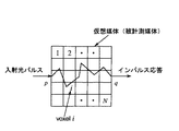
ここで、本発明の散乱吸収体内部の光路分布計算方法における「時間分解型光路分布」とは、図1に示すように、3次元の被計測媒体をN(1≦N)個のvoxe1(体積素)に分割した有限格子モデルとし、この有限格子モデルの光入射位置pからインパルス光を入射した場合に、有限格子モデルの光検出位置qにおいて計測されるインパルス応答の光路長がlとなる光子集合の光路分布を示す。具体的には、この時間分解型光路分布はvoxe1i(i=1,2,…,N;1≦N)の時間分解型光路長liを要素とするN次元ベクトル[li]で表される。上記の定義から、この時間分解型光路分布は光路長lの関数、つまり時間tの関数である。各種の具体的な計測法における出力光信号の減衰量は、この時間分解型光路長liとvoxe1iの吸収係数の積の関数で表される。また、この時間分解型光路長liの時間に対する加重平均Liは、voxe1iの平均光路長とよばれ、これを要素とするN次元ベクトル[Li]は平均光路長分布とよばれる。
【0039】
更に、重み関数は注目している物理量に対する吸収情報の寄与度として定義される。例えば、TRSで得られる時間分解型の減衰量に対する重み関数は、吸収や吸収分布に無関係となり、[時間分解型減衰量]=[重み関数]・[吸収係数差]となり、この重み関数は上記で求めた時間分解型光路長liに等しい。また、インパルス応答の時間積分(TRS)で得られる減衰量に対に重み関数は[TRS減衰量]=[重み関数]・[吸収係数差]で定義され、平均光路長差に対に対する重み関数は[平均光路長差]=[重み関数]・[吸収係数差]で定義される。TRSの場合、これらの重み関数は吸収係数の関数になる。
【0040】
このような重み関数を導入することによって、光CTにおける画像再構成のための行列式が行列の積、つまり[重み関数]・[吸収係数差]として記述され、この式から[吸収係数差]すなわち吸収分布を計算することができる。
【0041】
なお、上記の被計測媒体と仮想媒体との散乱特性は不均一であってもよく、順問題の具体的な計算には、モンテカルロ計算、経路積分(Path Integral)や輸送方程式の数値計算、光拡散方程式の数値計算などを利用することができる。
【0042】
ここで、本発明の散乱吸収体内部の光路分布計算方法により求めた時間分解型光路長liが適用される「所定の計測方式」とは、特に限定されるものではなく、例えば、発明者らがMBLに基づいて導出した時間分解計測(TRS)、時間積分計測(TIS)、時間分解ゲート積分計測(TGS)、更には周波数領域での位相変調計測(PMS)、平均値法に基づく光CT画像の再構成法(AVM)等の散乱吸収体の内部計測方法でもよく、先に文献(1)〜(12)に示したようなMBLに基づかない計測方法でもよい。
【0043】
また、本発明の散乱吸収体内部の光路分布計算方法は、
計測波長領域において、散乱吸収体である被計測媒体を、所定の大きさを有すると共に一様な吸収分布を有するとみなせるN(1≦N)個のvoxe1に分割する第1ステップと、
前記N個のvoxe1に分割された前記被計測媒体に対して、形状、境界条件及び散乱分布が前記被計測媒体と同一であり、屈折率分布が一様で、吸収がないとみなせる仮想媒体を仮定する第2ステップと、
前記仮想媒体の表面に、インパルス光が入射する光入射位置と、前記光入射位置から入射して前記仮想媒体内を伝播した前記インパルス光の時間tにおけるインパルス応答s(t)を検出する光検出位置とを設定する第3ステップと、
前記光入射位置から前記仮想媒体内にインパルス光を入射する場合に、前記光検出位置において時間tの時点で検出される前記インパルス応答s(t)を構成する光子集合が、前記光検出位置において検出される以前の時間t'(0≦t'≦t)の時点で前記仮想媒体内の任意のvoxe1i(i=1,2,…,N;1≦N)内に存在していた光子存在確率密度Ui(t',t)を算出する第5ステップと、
前記光子存在確率密度Ui(t',t)を使用して前記光検出位置において時間tの時点で検出される前記インパルス応答s(t)を構成する光子集合が前記voxe1i内に存在していた光子存在累積確率Ui(t)を算出する第6ステップと、
前記光子存在累積確率Ui(t)の全voxe1に対する総和U(t)を算出する第7ステップと、
前記光子存在累積確率Ui(t)及び前記光子存在累積確率Ui(t)の全voxe1に対する総和U(t)を使用して前記voxe1iの時間分解型光路長liを算出する第11ステップと、
を備えることを特徴とする方法である。
【0044】
上記の場合にも、voxeliの時間分解型光路長liを迅速且つ直接計算することができるので、これを用いて時間分解型光路長liの時間に対する加重平均Li を迅速に算出することができる。また、voxeliの時間分解型光路長liを迅速且つ直接計算することができるので、これを用いて被計測媒体内部における吸収成分の濃度分布を定量計測するための所定の各種の具体的な計測方法に対応する重み関数Wiを迅速に計算することができる。
【0045】
【発明の実施の形態】
以下、図面を参照しながら本発明による散乱吸収体内部光路分布計算方法の好適な実施形態について詳細に説明する。なお、以下の説明では、同一または相当部分には同一符号を付し、重複する説明は省略する。また、散乱吸収体内を散乱されつつ伝播する光子に関しては3次元座標を用いて考える必要があるが、以下では説明を簡単にするために場合により2次元座標を用いて説明する。
【0046】
先ず、本発明の原理について説明する。
[本発明の原理]
先に述べたように、本発明者らがMBLに基づいて開発してきた散乱媒体内の光の振る舞いを解析する解析法は、散乱や吸収が不均一に分布する不均一散乱媒体(不均一系)に適用することができる。そして、MBLに基づく解析法により、不均一散乱媒体の種々の光応答(光出力)が吸収に依存する減衰項と吸収に依存しない項とに分離して記述できること、更に、この光応答の減衰項が被計測媒体内の光路分布と吸収分布で記述できることが演繹される。従って、前もって被計測媒体内の光路分布を知ることができれば、被計測媒体内部の吸収成分の濃度分布を定量する光CTなどが可能になる。つまり、光CTを実現するには、被計測媒体内の光路分布を知ることと、光路分布を迅速に計算する方法を開発することが重要である。
【0047】
本発明は、被計測媒体及びこれに対応する仮想媒体の有限格子モデルにおいて、以下の(i)〜(v)の事柄が成立することを出発点としている。
【0048】
すなわち、(i)被計測媒体内の屈折率分布が一様であると仮定すれば、被計測媒体のインパルス応答(時間分解波形)では、光路長をlとし、屈折率で決まる被計測媒体中の光速度をc、時間をtとすれば、常にl=ctが成立する。ここで、被計測媒体内の屈折率分布が一様であると仮定するのは、被計測媒体として生体などの不均一散乱吸収体を選択した場合には、生体の主成分は水であるためその屈折率分布は一様であると見なしてよいからである。従って、以下の説明においては特にことわりがない限り屈折率分布が一様な被計測媒体を考える。
【0049】
(ii)散乱と吸収が独立であることから、散乱と吸収が任意に分布する不均一媒体に対して光入射位置、及び光検出位置を定めると、インパルス応答を構成する(インパルス応答として検出される)光子集合の光路分布、つまり時間分解型光路分布が一意的に決まる。
【0050】
(iii)上記の光路分布は、時間の関数となり、入射光子数(つまり光子密度)、被計測媒体の吸収や吸収分布に無関係であり、被計測媒体に吸収がないと仮定したときの光路分布に等しい。そして、3次元の被計測媒体を所定の大きさを有するN(1≦N)個のvoxe1(体積素)に分割した場合において、光路長がlとなる光子集合の光路分布は、各voxe1i(i=1,2,…,N;1≦N)の光路長liを要素とするN次元ベクトル[li]で表すことができる。
【0051】
(iv)この時間分解型光路分布[li]は、被計測媒体と同一の散乱特性(不均一であってよい)と境界条件をもつが、屈折率分布が一様で、且つ吸収がない仮想媒体を仮想して計算することができる。
【0052】
(v)各種の光CT画像再構成アルゴリズムに用いる各種の重み関数Wiを上記に定義した各voxe1iの時間分解型光路長liを用いて記述することができる。
なお、本発明者は、この時間分解型光路分布liを用いて記述される重み関数Wiと被計測媒体に対する実測値を用いて不均一媒体内の吸収成分の濃度分布を計測する光CTを提案した(特願平10−144300、文献(19))。
【0053】
図1は被計測媒体である不均一散乱吸収体の内部光子移動を解析するための有限格子モデルを示す。
【0054】
図1に示す有限格子モデルは、被計測媒体に対して形状、散乱分布、及び境界条件が同一であり、屈折率分布が一様、且つ吸収がないとして仮定される仮想媒体を示したものである。この際、3次元の被計測媒体をN(1≦N)個のvoxe1(体積素)に分割すると共にそれぞれのvoxe1に番号i(i=1,2,…,N;1≦N)を付けているので、被計測媒体に対応して仮定される仮想媒体も同様にN個のvoxe1を有している。
【0055】
また、図1に示す仮想媒体の有限格子モデルのvoxe1iの大きさ及び形状は、対応する被計測媒体のvoxe1i内の吸収分布が一様であると見なせるか、一様であると見なしてさしつかえない範囲及び形状で設定される。これは、実際の計測によって得られる各voxe1i内の吸収分布データは、各voxe1i内の吸収分布の平均値として得られるからである。voxe1iの大きさ及び形状が決まることにより全voxe1の総数も決まる。すなわち、仮想媒体のvoxe1iの大きさ、形状、及び全voxe1の総数は、先に述べたのようにvoxe1i内の吸収が一様であると見なせる限りにおいて任意である。実際のvoxe1iの大きさ及び形状は、使用される計測方式、或いはそれらの計測方式に要求されるCT画像の解像度に応じて決定される。
【0056】
本発明の散乱吸収体内部の光路分布計算方法においては、図1に示す仮想媒体の有限格子モデルの光入射位置pからインパルス光を入射した場合に、有限格子モデルの光検出位置qにおいて計測されるインパルス応答の中で、光路長がlとなる光子集合を考える。ここで、光子入射位置p、光子検出位置qは任意である。
【0057】
図1に示す有限格子モデルに多数の光子からなるインパルス光を入射した場合のインパルス応答には、種々の光路長をもつ光子が含まれるが、観測時間tを決めるとl=ctとして光路長lが一意的に決まる。そして、光路長がlとなる光子は多数存在する。そこで、この光路長がlとなる光子集合の光路分布、すなわちvoxe1i(i=1,2,…,N;1≦N)における光路長liを、光子が取り得る光路の確率分布で示すことと定義する。これに伴い有限格子モデル内のvoxe1iの光路分布は、voxe1i内の時間分解型光路長liを要素とするN次元ベクトル[li]で表される。なお、先に述べたように光路長がlとなる光子は多数存在するから、voxe1i内の時間分解型光路長liは、これらの個々の光子のvoxe1i内の光路長の平均(集合平均)である。また、このような系では、光入射位置pと光検出位置qを定めると、インパルス応答を構成する光子集合の時間分解型光路分布[li]が一意的に決まる。
【0058】
ここで、上記の被計測媒体のインパルス応答を構成する光子集合の時間分解型光路分布[li]は被計測媒体の吸収に無関係であるので、吸収がないと仮定したときの仮想媒体のインパルス応答を構成する光子集合の時間分解型光路分布[li]に等しい。すなわち、仮想媒体のインパルス応答を構成する光子集合の時間分解型光路分布[li]を求めることにより、被計測媒体のインパルス応答を構成する光子集合の時間分解型光路分布[li]を求めることができる。
【0059】
1. 解析モデルと解析の概要
まず、不均一散乱媒体である被計測媒体における減衰量、光路長などの関係を説明する。吸収と散乱は独立であるから、ここでは、図1に示す有限格子モデルが被計測媒体と同一の吸収分布をもつと仮定すれば良い。ただし、その他の条件は仮想媒体の有限格子モデルと同じである。
【0060】
すると、まず上記の(i)ないし(v)の知見と、MBLから、光路長lと光路長分布liとの関係は、下記式で表現される。
【数3】
【0061】
また、不均一散乱媒体を被計測媒体としたときの光路長がlとなる光子集合のインパルス応答は、(1)式に対応する下記式で表現される。
【数4】
【0062】
(4)式及び(5)式は、それぞれ(3)式で表現されるインパルス応答を微分形と積分形で表示したものである。(5)式より不均一散乱媒体のインパルス応答h(t)が吸収に依存しない項ln s(t)と下記式で表される吸収に依存する減衰項とに分離して記述できることがわかる。
【数7】
更に、(5)式より、この光応答の減衰量 ln[h(t)/s(t)] が被計測媒体内の時間分解型光路分布 [li] と吸収分布 [μai] とで記述できることがわかる。なお、ここで、被計測媒体内の時間分解型光路分布は、前記仮想媒体内、つまり吸収がないときの時間分解型光路分布に等しいことに注意する必要がある。従って、時間分解型の計測(TRS)では、減衰量に対する重み関数は時間分解型光路長分布 [li] に等しく、この関係を利用した光CT画像再構が可能になる。なお、このような時間分解型光CTは、画像再構成アルゴリズムが最も簡単になる。
【0064】
より一般的な光CTとしては、上記インパルス応答の時間積分値を利用するTIS、インパルス応答の所定時間範囲内の積分値を利用するTGS、正弦波変調光を利用するPMS、更には、これら各種の方法において、仮想媒体に基準となる均一な吸収を与え、その基準値からの偏差を計測するAVMがる。ところが、これらの全ての方法に対して、減衰量あるいは減衰量偏差が吸収に依存する減衰項と吸収に依存しない項とに分離して記述できること、更に、各種の光応答の減衰量あるいは減衰量偏差が被計測媒体内の時間分解型光路分布と吸収分布で記述できることが導出され、この関係から減衰量あるいは減衰量偏差に対する重み関数を求めることができる。また、後述するように、減衰量あるいは減衰量偏差がキュムラント関数であることを利用すると、TISやPMSにおける重み関数が平均光路長や位相遅延およびキュムラントで記述できることが導出される。
【0065】
例えば、TISの場合における光応答は、前述のインパルス応答h(t)の時間積分に相当し、下記式のように表現できる。
【数8】
【0066】
また、(6)式の微分形及び積分形は、(3)式に対応する(4)式及び(5)式と同様に下記式のように表現できる。
【数9】
【0067】
この平均光路長(時間分解型光路長liの加重平均)Liは、散乱体の散乱特性、境界条件、及び吸収や吸収分布に依存する。この際、(8)式の右辺第2項の積分は、(5)式のように積で表示することができないことに注意する必要がある。従って、減衰量に対する重み関数は、単なる平均光路長Liではなく、吸収に依存することになり、このことが光CT再構成アルゴリズムを複雑にしている。
【0068】
また、仮想媒体に基準となる均一な吸収を与え、その基準値からの偏差として被計測媒体を計測するAVM計測では、voxe1iにおける被計測媒体と仮想媒体との減衰量差(減衰量偏差)(Bi は、吸収係数差(吸収係数偏差)(μai 、重み関数 Wi を用いて下記式のように表現される。
【数11】
Δμaiは、μνに対するμaiの吸収係数偏差を示し、
Bi(μai)は、被計測媒体のvoxe1iのインパルス応答の時間積分Iに関する減衰量を示し、
Bi(μν)は、仮想媒体のvoxe1iのインパルス応答の時間積分Iに関する減衰量を示し、
ΔBi(μai)は、Bi(μν)に対するBi(μai)の減衰量偏差を示し、
Li(μν)は、仮想媒体のvoxe1iの平均光路長の差(時間積分Iに関する平均光路長の差)を示し、voxe1i内の時間分解型光路長liの加重平均に等しい、
Wiは、減衰量偏差ΔBi(μai)に対する重み関数であり、吸収係数偏差Δμai及びキュムラント(L, L',L",…)の関数をで表される。]
ここで、キュムラントは、仮想媒体に対して求めた時間分解波形から直接算出することができる。
【0069】
また、上記の計測方法の他に各種の光CTに応じて誘導される他の諸量、例えば、光路長平均の差と光路長分散に対応する重み関数との組み合わせを使用しても光路長平均の差と光路長分散に対応する重み関数との間には上記の(9)式と同様の関係式が成立し、吸収係数分布を定量計測することができる。具体的には波長の異なる光に対してこの計測を行い、得られた吸収係数と物質に固有の吸光係数から、吸収成分の濃度分布(絶対値)を定量計測する。
【0070】
2.時間分解型光路長の計算方法
次に、有限格子モデルで記述される仮想媒体に対して、時間分解型光路分布[li]の要素である時間分解型光路長liを算出する式を導出する。
更に、この時間分解型光路長liから、TIS(時間分解積分方式)、TGS(時間分解ゲート積分方式)、及びPMS(位相変調方式)の光CTに用いる計測方法に対応する各種の重み関数を計算することができるので、これらの具体例についても説明する。
【0071】
被計測媒体のvoxe1iの有する吸収係数はμaiであるが、仮想媒体の有限格子モデルのvoxe1iの有する吸収係数は、μai=0である。このとき、図1に示す仮想媒体の有限格子モデルのインパルス応答は、(3)式にμai=0を代入して、下記式のように表現される。
【数18】
【0072】
このとき、時間分解型光路長liと光路長lとの関係は下記式で表現できる。
【数19】
【0073】
上記の時間分解型光路長liと光路長lとの関係は、一個の光子がジグザグに伝播して同じvoxe1を2回以上通過した場合でも成立する。なお、上式においては、総光路長lと各voxe1iの時間分解型光路長liが時間tの関数であることを明示するため、それぞれを「l(t)」、「li(t)」と表記した。
【0074】
以下、このようなtをパラメトリック変数として、voxe1iの時間分解型光路長liを算出する原理とその過程について詳細に説明する。
【0075】
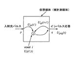
図2は、図1に示す有限格子モデルにおいて、光入射位置pからインパルス光を入射して伝播光を光検出位置qで検出する場合、インパルス応答s(t)を構成し且つ光路長がlとなる光子集合(すなわち、時間tの時点で検出される光子集合)のうち、voxe1iを通過した光子集合の経路と確率密度、およびそのような光子集合が光検出位置qにおいて時間tの時点で検出される値Upiq(t)とを示す模式図である。
【0076】
ここで、上記有限格子モデルにおいて、光入射位置pからインパルス光を入射して伝播光を光検出位置qで検出する場合、インパルス応答s(t)を構成し且つ光路長がlとなる光子集合(すなわち、時間tの時点で検出される光子集合)が、光検出位置qにおいて検出される以前の時間t'(0≦t'≦t)の時点にvoxe1iに存在する光子存在確率密度Ui(t',t)を考える。なお、以下の説明において、このような光子存在確率密度Ui(t',t)を、単に「時間t'におけるvoxe1i内の光子存在確率密度Ui(t',t)」として記述する。
【0077】
このとき、上記の新しい時間変数t'を導入して記述される時間t'におけるvoxe1i内の光子存在確率密度Ui(t',t)は、相反原理(reciprocity theorem)を適用することにより下記式のように表現できる。
【数20】
Uqi(t-t')は、時間t-t'=0において光検出位置qから入射した光子が時間t-t'においてvoxe1i内に存在する光子存在確率密度を示す。]
【0078】
生体のような散乱媒体では、コリメート光入射やペンシルビーム入射に対して近似的に相反原理が成立するが、より厳密に相反原理を適用する場合には、等方光入射と呼ばれる光入射方法を利用することが好ましい。これは等方光入射法においては、相反原理がより精度よく成立するからである。なお、この等方光入射法は、発明者が既に報告した光入射方法であり、例えば、特願平5−301979、Y. Tsuchiya, K.Ohta, and T. Urakami: Jpn.J.Appl. Phys.34, Part 1, pp.2495-2501(1995)に開示されている。
【0079】
また、以下の説明において、上記の(2.2)式で示されるUpi(t')とUqi(t-t')とを、それぞれ、単に「時間t'におけるvoxe1i内の光子存在確率密度Upi(t')」、「時間t-t'におけるvoxe1i内の光子存在確率密度Uqi(t-t')」として記述する。
【0080】
図3は、上記の(2.2)式で示される有限格子モデル内の時間t'におけるvoxe1i内の光子存在確率密度Ui(t',t)、時間t'におけるvoxe1i内の光子存在確率密度Upi(t')、及び、時間t-t'におけるvoxe1i内の光子存在確率密度Uqi(t-t')の一例を示すグラフである。
【0081】
上記のUi(t',t)は、(2.2)式で示される二つの順問題を計算することにより算出することができる。この時、Upi(t')は、有限格子モデルの光入射位置pからインパルス光を入射して計算することができる。また、Uqi(t-t')も有限格子モデルの光検出位置qからインパルス光を入射して計算することができる。なお、上記の順問題の具体的な計算には、モンテカルロ計算、経路積分(Path Integral)や輸送方程式の数値計算、光拡散方程式の数値計算などを利用することができる。この際、上記有限格子モデルでは吸収がないから、従来の吸収がある場合の順問題計算より計算アルゴリズムが簡単になり、計算時間も短くなる。
【0082】
上記の時間t'におけるvoxe1i内の光子存在確率密度Ui(t',t)を算出することにより、有限格子モデル内に光入射位置pからインパルス光を入射する場合に、光検出位置qにおいて時間tの時点で検出されるインパルス応答s(t)を構成する光路長がlとなる光子集合が、光入射位置pから光検出位置qへと有限格子モデル内を伝播する時間0≦t'≦tの間にvoxe1iに存在する確率密度Ui(t)を下記式に従って算出することができる。この確率密度Ui(t)には、有限格子モデル内(仮想媒体内、被計測媒体内)をジグザグに伝播する光子が異なる時間に同一のvoxelに存在した場合の確率が累積されている。
【数21】
上記の(2.3) 式で示されるUi(t)はインパルス応答s(t)を構成し、且つ光路長がlとなる光子集合のvoxe1i内の光子存在累積確率を表しており、以下の説明において、単に「時間0≦t'≦tにおけるvoxe1i内の光子存在累積確率Ui(t)」として記述する。
【0084】
ここで、有限格子モデル内の全voxe1について(2.3)式で示される光子存在累積確率Ui(t)の総和をとり、有限格子モデル内の光子存在累積確率U(t)を求めると、次式が得られる。
【数22】
この光子存在累積確率U(t)は、有限格子モデル内に光入射位置pからインパルス光を入射する場合に、光検出位置qにおいて時間tの時点で検出されるインパルス応答s(t)を構成する光路長がlとなる光子集合が、光入射位置pから光検出位置qへと有限格子モデル内を伝播する時間0≦t'≦tの間に有限格子モデル内(全voxe1内)に存在する累積確率を表わす。
【0086】
以下の説明において、上記の(2.4) 式で示されるU(t)を、「時間0≦t'≦tにおける全voxe1内の光子存在累積確率U(t)」として記述する。
【0087】
一方、先に述べた時間t'におけるvoxe1i内の光子存在確率密度Ui(t',t)に対して、有限格子モデル内に光入射位置pからインパルス光を入射する場合に、光検出位置qにおいて時間tの時点で検出されるインパルス応答s(t)を構成する光路長がlとなる光子集合が、光検出位置qにおいて検出される以前の時間t'(0≦t'≦t)の時点に有限格子モデル内(仮想媒体内)に存在する確率密度Upq (t',t)を考える。すなわち、「時間t'におけるvoxe1i内の光子存在確率密度Ui(t',t)」に対して、「時間t'における全voxe1内の光子存在確率密度Upq(t',t)」を考える。この場合、時間t'における光子存在確率密度を考えているから、全voxe1に対する光子存在確率密度の総和はUpq(t',t)に等しく、このUpq(t',t)はUi(t',t)を用いて下記式で表現することができる。
【数23】
この(2.5)式を時間t'= 0 から時間 t'= t の範囲で定積分したものは、当然、先に求めた時間 0≦t'≦tにおける全voxe1内の光子存在累積確率U(t)に等しく、下記式で表現することができる。
【数24】
ここで、本発明の散乱吸収体内部の光路分布計算方法においては、吸収がない仮想媒体を考えているから、時間t'における全voxe1内の光子存在確率密度Upq(t',t)は、時間t'=0から時間t'=tまで一定である。そこで、累積確率U(t)は、(2.6)式を用いて下記式のように表現することができる。
【数25】
上記の事実に加えて、吸収がない仮想媒体において時間t'における全voxe1内の光子存在確率密度Upq(t',t)は、時間t'=0から時間t'=tまで一定であることから、このUpq(t',t)は、光検出位置qにおいて時間tの時点で検出されるインパルス応答、つまり(1.1)式に求めたs(t)に等しいことがわかる。すなわち、Upq(t',t)とs(t)との関係が、下記式のように表現される。
【数26】
以上から、(2.4)式の時間0≦t'≦tにおける全voxe1内の光子存在累積確率U(t)は(2.8)式の結果を(2.7)式に代入することにより最終的に下記式で表現される。
【数27】
更に、前出の図2で説明したUpiq(t)の全voxe1に対する総和は、有限格子モデル内の光子存在累積確率U(t)に等しく、下記式で示す関係が成り立つことが理解される。
【数28】
なお、図4に上記の時間0≦t'≦tにおけるvoxe1i内の光子存在累積確率Ui(t)、時間t'におけるvoxe1i内の光子存在確率密度Ui(t',t)、及び、時間t'における全voxe1内の光子存在確率密度Upq(t',t)の関係を模式的に示す。
また、有限格子モデル内に光入射位置pからインパルス光を入射する場合に、光検出位置qにおいて時間tの時点で検出されるインパルス応答s(t)を構成する光子集合の中で光路長がlとなる光子集合の時間t'におけるvoxeli内の時間分解型光路長をli(t',t)とすれば、このli(t',t)を時間t'= 0 から時間 t'= t まで積分したものが、時間分解型光路長li(t)に等しく、下記式で表現することができる。
【数29】
ところで、有限格子モデル内の光速度は一定であるから、任意の時間あるいは任意の部分を考えた場合、光路長と格子存在確率は常に比例する。
【0095】
具体的には、有限格子モデル内に光入射位置pからインパルス光を入射する場合に、光検出位置qにおいて時間tの時点で検出されるインパルス応答s(t)を構成する光子集合の中で光路長がlとなる光子集合を考えた場合、任意の時間t'におけるvoxeli内の時間分解型光路長をli(t',t)は、時間t'におけるvoxe1i内の光子存在確率密度Ui(t',t)に比例する。そして、li(t',t)の時間積分値である時間分解型光路長li(t)もUi(t',t)の時間積分値である光子存在累積確率Ui(t)に比例する。更には、有限格子モデル内に光入射位置pからインパルス光を入射する場合に、光検出位置qにおいて時間tの時点で検出されるインパルス応答s(t)を構成する光子集合の中で光路長がlとなる光子集合を考えた場合、光路長lは光子存在累積確率U(t)に比例する。
【0096】
この比例係数をAとおけば、(2.1)式、(2.9)式、および(2.11)式などの関係から下記式を得ることができる。
【数30】
【0097】
(2.12)式の関係を同値変形して時間分解型光路長li(t)について解くと下記式が得られる。
【数31】
【0098】
なお、このような時間分解型光路長liは、時間分解応答を利用する時間分解型光CTの画像再構成に直接的に用いられる。つまり、時間分解型光CTにおける重み関数は、時間分解型光路長光路長liに等しいからである。また、後述するように、時間分解型光路長liは、各種の計測法式における重み関数を記述するための基本量となる。
【0099】
3.時間分解型光路長liの具体的計算法
図5は、本発明の散乱吸収体内部の光路分布計算方法の一実施形態を示すフローチャートである。以下、図5に示すフローチャートについて説明する。
【0100】
先ず、計測波長領域において、散乱吸収体である被計測媒体を、所定の大きさを有すると共に一様な吸収分布を有するとみなせるN(1≦N)個のvoxe1に分割する(S1)。
【0101】
次に、N個のvoxe1に分割された被計測媒体に対して、形状、境界条件及び散乱分布が被計測媒体と同一であり、屈折率分布が一様で、且つ吸収がないとみなせる仮想媒体を仮定する(S2)。
【0102】
次に、仮想媒体の表面に、インパルス光が入射する光入射位置pと、光入射位置pから入射して仮想媒体内を伝播したインパルス光の時間tにおけるインパルス応答s(t)を検出する光検出位置qとを設定する(S3)。
【0103】
次に、仮想媒体内へ光入射位置pからインパルス光を入射させ、光検出位置において検出されるインパルス応答s(t)を算出する(S4)。
【0104】
次に、光入射位置pから仮想媒体内にインパルス光を入射し、時間t'=0において光入射位置pから入射した光子が時間t'=t'においてvoxe1i内に存在する光子存在確率密度Upi(t')を計算する。続いて、光検出位置qから仮想媒体内にインパルス光を入射し、時間t-t'=0において光検出位置qから入射した光子が時間 t-t'においてvoxe1i内に存在する光子存在確率密度Uqi(t-t')を計算する。そして、(2.2)式に従って、有限格子モデル内に光入射位置pからインパルス光を入射する場合に、光検出位置において時間tの時点で検出されるインパルス応答s(t)を構成する光路長がlとなる光子集合が、光検出位置において検出される以前の時間t'(0≦t'≦t)の時点にvoxe1iに存在する光子存在確率密度Ui(t',t)を計算する(S5)。
【0105】
以上の場合、一個の光入射位置に対して、有限格子モデルを構成する全voxe1の光子存在確率密度を並列あるいは同時に計算することができる。そのため、各voxelの吸収係数を変化させて、voxe1の総数Nに等しい回数だけ順問題を繰り返して解くという時間のかかる従来型の計算が不要になり、計算時間が著しく短縮される。
【0106】
次に、(2.3)式に従って、光子存在確率密度Ui(t',t)から光検出位置qにおいて時間tの時点で検出されるインパルス応答を構成する光子集合がvoxe1i内に存在していた光子存在累積確率Ui(t)を算出する(S6)。
【0107】
最後に(2.13)式に従って光子存在累積確率Ui(t)及びインパルス応答s(t)を使用し、voxe1iの時間分解型光路長liを計算する(S8)。
【0108】
以上の本発明の第一実施形態において説明されるように、本発明の散乱吸収体内部の光路分布計算方法は、被計測媒体と同一の散乱特性と境界条件をもつが、吸収がないと仮定した仮想媒体に対して(2.2)式に示す順問題を解くので、従来の吸収があるときの順問題計算比べて、計算時間が短くなる。更に、各voxelの吸収係数を変化させてvoxe1の総数に等しい回数だけ順問題を繰り返して解くという時間のかかる従来の題計算が不要になり、voxe1i内の時間分解型光路長liを直接且つ迅速に計算することができる。
【0109】
また、上記の散乱吸収体内部の光路分布計算方法を各種の光応答を用いた光CTに適用する場合には、図5に示すフローチャートの後段において、仮想媒体の任意のvoxe1iごとに算出される時間分解型光路長liを使用して、被計測媒体内部における吸収成分の濃度分布を定量計測するための所定の計測方式に対応する重み関数Wiを算出する。この場合には、仮想媒体の任意のvoxe1iごとに算出される時間分解型光路長liから所定の計測方式に対応する重み関数Wiを直接算出する方法と、はじめに仮想媒体の任意のvoxe1iごとに算出される時間分解型光路長liの時間に対する加重平均Liを求め、この加重平均Liを使用して所定の計測方式に対応する重み関数Wiを算出する方法とがある。
【0110】
先にも述べたように、従来は、時間分解型光路長liの具体的な計算方法が知られていなかったため、最初に時間分解型光路長liを求めて、その後で、時間分解型光路長liの加重平均Li及び重み関数Wiを算出するという発想がなかったのに対し、この重み関数の計算方法は、voxeliの時間分解型光路長liを迅速且つ直接計算することができるので、これを用いて時間分解型光路長liの加重平均Li或いは被計測媒体内部における吸収成分の濃度分布を定量計測するための所定の各種の具体的な計測方法に対応する重み関数Wiを迅速に計算することができる。なお、仮想媒体の任意のvoxe1iごとに算出される時間分解型光路長liを使用した各種の光応答を用いた光CTに対応する重み関数の具体的計算方法については後述する。
【0111】
図6は、本発明の散乱吸収体内部の光路分布計算方法の第二の実施形態を示すフローチャートである。以下、図6に示すフローチャートについて説明する。
【0112】
先ず、計測波長領域において、散乱吸収体である被計測媒体を、所定の大きさを有すると共に一様な吸収分布を有するとみなせるN(1≦N)個のvoxe1に分割する(S1)。
【0113】
次に、N個のvoxe1に分割された被計測媒体に対して、形状、境界条件及び散乱分布が被計測媒体と同一であり、屈折率分布が一様で、且つ吸収がないとみなせる仮想媒体を仮定する(S2)。
【0114】
次に、仮想媒体の表面に、インパルス光が入射する光入射位置pと、光入射位置pから入射して仮想媒体内を伝播したインパルス光の時間tにおけるインパルス応答s(t)を検出する光検出位置qとを設定する(S3)。
【0115】
次に、光入射位置pから仮想媒体内にインパルス光を入射し、時間t'=0において光入射位置pから入射した光子が時間t'=t'においてvoxe1i内に存在する光子存在確率密度Upi(t')を計算する。続いて、光検出位置qから仮想媒体内にインパルス光を入射し、時間t-t'=0において光検出位置qから入射した光子が時間t'-tにおいてvoxe1i内に存在する光子存在確率密度Uqi(t-t')を計算する。そして、(2.2)式に従って、有限格子モデル内に光入射位置pからインパルス光を入射する場合に、光検出位置において時間tの時点で検出されるインパルス応答s(t)を構成する光路長がlとなる光子集合が、光検出位置において検出される以前の時間t'(0≦t'≦t)の時点にvoxe1iに存在する光子存在確率密度Ui(t',t)を計算する(S5)。
【0116】
以上の場合にも、一個の光入射位置に対して、有限格子モデルを構成する全voxe1の光子存在確率密度を並列あるいは同時に計算することができる。そのため、各voxelの吸収係数を変化させて、voxe1の総数Nに等しい回数だけ順問題を繰り返して解くという時間のかかる従来型の計算が不要になり、計算時間が著しく短縮される。
【0117】
次に、(2.3)式に従って、光子存在確率密度Ui(t',t)から光検出位置qにおいて時間tの時点で検出されるインパルス応答を構成する光子集合がvoxe1i内に存在していた光子存在累積確率Ui(t)を算出する(S6)。
【0118】
続いて、(2.4)式に従って、光子存在累積確率Ui(t)の全voxe1に対する総和U(t)を算出する(S7)。
【0119】
最後に(2.13)式に従って光子存在累積確率Ui(t)及びインパルス応答U(t)を使用し、voxe1iの時間分解型光路長liを計算する(S11)。
【0120】
以上の本発明の第二実施形態の説明から、先に述べた本発明の第一実施形態の説明と同様に、本発明の散乱吸収体内部の光路分布計算方法は、被計測媒体と同一の散乱特性と境界条件をもつが、吸収がないと仮定した仮想媒体に対して(2.2)式に示す順問題を解くので、従来の吸収があるときの順問題計算比べて、計算時間が短くなることがわかる。更に、各voxelの吸収係数を変化させてvoxe1の総数に等しい回数だけ順問題を繰り返して解くという時間のかかる従来の題計算が不要になり、voxe1i内の時間分解型光路長liを直接且つ迅速に計算することができることがわかる。
【0121】
また、先に説明した本発明の第一実施形態と同様、上記の散乱吸収体内部の光路分布計算方法を各種の光応答を用いた光CTに適用する場合には、図6に示すフローチャートの後段において、仮想媒体の任意のvoxe1iごとに算出される時間分解型光路長liを使用して、被計測媒体内部における吸収成分の濃度分布を定量計測するための所定の計測方式に対応する重み関数Wiを算出する。この場合にも、仮想媒体の任意のvoxe1iごとに算出される時間分解型光路長liから所定の計測方式に対応する重み関数Wiを直接算出する方法と、はじめに仮想媒体の任意のvoxe1iごとに算出される時間分解型光路長liの時間に対する加重平均Liを求め、この加重平均Liを使用して所定の計測方式に対応する重み関数Wiを算出する方法とがある。
【0122】
この重み関数の計算方法は、voxeliの時間分解型光路長liを迅速且つ直接計算することができるので、これを用いて時間分解型光路長liの加重平均Li或いは被計測媒体内部における吸収成分の濃度分布を定量計測するための所定の各種の具体的な計測方法に対応する重み関数Wiを迅速に計算することができることになる。
【0123】
以上説明したように、本発明の散乱吸収体内部の光路分布計算方法は各種の光応答を用いた光CTに適用することができる。この場合には、図5或いは図6に示すフローチャートの後段において、仮想媒体の任意のvoxe1iごとに算出される時間分解型光路長liを使用して、被計測媒体内部における吸収成分の濃度分布を定量計測するための所定の計測方式に対応する重み関数Wiを算出する。
【0124】
例えば、具体例としては発明者らがMBLに基づいて導出した時間積分計測(TIS)、及び時間分解ゲート積分計測(TGS)、周波数領域での位相変調計測(PMS)、更には平均値法(TIS)等がある。これらの場合、各種の光応答は、先に述べたインパルス応答の数学変換で定義されるが、それぞれに対応する光CTでは、それぞれに異なった重み関数を用いる。
【0125】
以下、時間積分計測(TIS)、時間分解ゲート積分計測(TGS)、及び周波数領域での位相変調計測(PMS)等の光応答を用いた光CTに本発明の散乱吸収体内部の光路分布計算方法により求めた時間分解型光路長liを適用する例について説明する。
【0126】
4.TISにおける散乱吸収体内部の光路分布と重み関数
先に述べたように、インパルス応答h(t)の時間積分Iを用いるTISに基づく光CTでは、インパルス応答h(t)に対するvoxel i の平均光路長Liや光路長分散などを用いて記述される重み関数を用いる。なお、この重み関数Wiは、吸収分布が一様な基準媒体に対する重み関数として定義される。
【0127】
まず、吸収が不均一に分布する散乱媒体のインパルス応答h(t)の時間積分Iを考える。この際に考えるモデルは、図1に示したモデルのvoxel i の吸収係数をμaiとしたものである。これらを用いて、インパルス応答の時間積分Iは、下記式で与えられる。
【数32】
s(t)は、被計測媒体に吸収がないと仮定したときに検出位置において検出されるインパルス応答を示し、
Liは、検出位置において検出された時間積分Iを構成する光子集合のvoxel i における平均光路長(voxeliにおける時間分解型光路長liの加重平均)を示す。]
この式では、lnIが吸収に無関係な項と、各voxelの吸収係数μaiに依存する項(減衰量)とに分離して記述されている。
【0128】
ここで、voxel i の平均光路長Liは、散乱体の散乱特性、境界条件、及び吸収や吸収分布に依存する量であり、下記式により与えられる。
【数33】
対応する光CTに用いる重み関数Wiは、均一な吸収係数μνをもつ仮想媒体に対して定義され、下記式により与えれる。この場合のモデルは、図1に示したモデルのvoxel i の吸収係数をμνとしたものである。
【数34】
Δμaiは、μνに対するμaiの吸収係数偏差を示し、
Li(μν)は、一定の吸収係数μνをもつ仮想媒体のvoxe1iにおける平均光路長を示し(voxe1i内の時間分解型光路長liの加重平均)、
L(μν)は、一定の吸収係数μνを与えた仮想媒体のインパルス応答の平均光路長を示し(仮想媒体内の光路長lの加重平均)、
Wiは、先に述べた(9)式中の減衰量偏差ΔBi(μai)に対する重み関数であり、吸収係数偏差Δμai及びキュムラント(L, L',L",…)の関数で表される。]
ここで、キュムラントは、仮想媒体に対して求めた時間分解波形から直接算出することができる。
【0130】
5.TGSにおける散乱吸収体内部の光路分布と重み関数
まず、吸収が不均一に分布する散乱媒体のインパルス応答の時間分解ゲート積分信号Igは、下記式で与えられる。
【数38】
ここで、ゲート積分の時間範囲は[t1,t2]であり、これを[0,∞]にすると、前節に求めたインパルス応答h(t)の時間積分信号Iになる。
【0131】
対応する光CTに用いる重み関数Wgiは、均一な吸収係数μνをもつ仮想媒体に対して定義され、下記式で与えられる。
【数39】
Δμaiは、前述の(4.4)式に示したように、μνに対するμaiの吸収係数偏差を示し、
Lgi(μν)は、仮想媒体のインパルス応答の時間ゲート積分Igを構成する光子集合のvoxel i における平均光路長(voxe1i内のゲート時間内における時間分解型光路長liの加重平均)を示し、
Lg(μν)は、一定の吸収係数μνを与えた仮想媒体のインパルス応答の時間ゲート積分Igを構成する光子集合の平均光路長(加重平均)を示し
Wiは、先に述べた(9)式の減衰量偏差ΔBi(μai)をTGSに適用したときの減衰量偏差ΔBgi(μai)に対する重み関数であり、吸収係数偏差Δμai及びキュムラント(Lg, Lg',Lg",…)の関数で表される。]
【0132】
6.PMSにおける散乱吸収体内部の光路分布と重み関数
吸収が不均一に分布する散乱媒体に対して、PMSで得られる応答は、吸収が不均一に分布する散乱媒体に対するインパルス応答h(t)をフーリエ変換したものであり下記式で与えられる。
【数42】
【数44】
[式(6.1)〜(6.6)中、R及びXはそれぞれ実数部と虚数部を示し、A及びφはそれぞれ振幅及び位相遅れを示す。]
R、X、A及びφは、ロックインアンプなどで容易に計測することができる。
【0133】
また、ここで、
【数48】
【数52】
【0134】
以上のように、PMSでは(6.7)式〜(6.10)式に示す4種類の記述方法があり、それぞれの式に対応する光CT画像再構成法が可能である。その際、先に述べたのと同様にして、(6.7)式〜(6.10)式にμai=μνを代入して求めた値と、(6.11)式〜(6.14)式の関係を用いて、それぞれの重み関数を算出することができる。
【0135】
以上、本発明の好適な実施形態について詳細に説明したが、本発明は上記実施形態に限定されない。
【0136】
【発明の効果】
以上説明したように、本発明によれば、被計測媒体と同一の散乱特性と境界条件をもつが、吸収がないと仮定した仮想媒体に対して順問題を解いて、voxe1i内の時間分解型光路長liを直接且つ迅速に計算することができるので、従来の吸収があるときの順問題計算比べて、計算時間が短くなる。更に、各voxelの吸収係数を変化させてvoxe1の総数に等しい回数だけ順問題を繰り返して解くという時間のかかる従来の順問題計算が不要になる。従って、生体などの不均一系の散乱吸収体内部の光路分布を迅速に算出することのできる方法を提供することが可能となる。
【図面の簡単な説明】
【図1】被計測媒体の内部光子移動を解析するための有限格子モデルを示す模式図である。
【図2】図1に示す有限格子モデルにおいて、光入射位置pからインパルス光を入射する場合に、光検出位置qにおいて時間tの時点で検出されるインパルス応答を構成する光子集合(光路長がlになる)のうち、voxe1iを通過した光子集合の経路とその確率を示す模式図である。
【図3】図2に示す有限格子モデル内の時間t'におけるvoxe1i内の光子存在確率密度Ui(t',t)、時間t'におけるvoxe1i内の光子存在確率密度Upi(t')、及び、時間t'におけるvoxe1i内の光子存在確率密度Uqi(t-t')の時間波形の一例を示すグラフである。
【図4】時間0≦t'≦tにおけるvoxe1i内の光子存在累積確率Ui(t)、 時間t'におけるvoxe1i内の光子存在確率密度Ui(t',t)、及び、時間t'における全voxe1内の光子存在確率密度Upq(t',t)の関係を模式的に示すグラフである。
【図5】本発明の散乱吸収体内部の光路分布計算方法の一実施形態を示すフローチャートである。
【図6】本発明の散乱吸収体内部の光路分布計算方法の第二の実施形態を示すフローチャートである。
【符号の説明】
S1…第1ステップ、S2…第2ステップ、S3…第3ステップ、S4…第4ステップ、S5…第5ステップ、S6…第6ステップ、S7…第7ステップ、S8…第8ステップ、S11…第11ステップ。[0001]
BACKGROUND OF THE INVENTION
The present invention relates to a method for calculating an optical path distribution inside a scattering medium. More specifically, calculation of the time-resolved optical path distribution inside the scattering medium that can be applied to a device that obtains information inside the measurement object by moving the light incident position and light detection position along the surface of the measurement object. Regarding the method.
[0002]
From this time-resolved optical path distribution, it is possible to calculate the optical path distribution in an appropriate measurement method, and to calculate the contribution (also referred to as a contribution function or weight function) of each part of the scattering medium with respect to the light attenuation amount and the average optical path length.
[0003]
[Prior art]
Conventionally, in a field such as optical CT in a broad sense including internal measurement, a measurement method for obtaining internal information of a measurement object using a weight function or a contribution function has been known. Many reports have been made. These are described in the following documents, for example.
[0004]
(1) S. Arridge: SPIE Institutes for Advanced Optical Technologies, Vol. IS11, Medical Optical Tomography: Functional Imaging and Monitoring, 35-64 (1993); (2) RL Barbour and HL Graber: ibid. 87-120 (1993) ); (3) HL Graber, J. Chang, R. Aronson and RL Barbour: ibid. 121-143 (1993); (4) JC Schotland, JC Haselgrove and JS Leigh: Applied Optics, 32, 448-5453 (1993) ); (5) Chang, R. Aronson, HL Graber and RL Barbour: Proc.SPIE, 2389, 448-464 (1995); (6) BW Pogue, MS Patterson, H. Jiang and KD Paulsen: Phys. Med. Biol. 40, 1709-1729 (1995); (7) SR Arridge: Applied Optics, 34, 7395-7409 (1995); (8) HL Graber, J. Chang, and RL Barbour: Proc.SPIE, 2570, 219 -234 (1995); (9) A. Maki and H. Koizumi: OSA TOPS, Vol. 2, 299-304 (1996); (10) H. Jiang, KD Paulsen and Ulf L. Osterberg: J. Opt. Soc. Am. A13, 253-266 (1996); (11) SR Arridge and JC Hebden: Phys. Med. Biol. 42, 841-853 (1997); (12) SB Colak, DG Papaioannou, GW 't Hooft , MB van der Mark, H. Schomberg, JCJ Paasschens, JBM Melissen and NAAJ van Astten: Appl ied Optics, 36, 180-213 (1997).
[0005]
However, the internal information measurement methods such as optical CT disclosed in the above-mentioned documents (1) to (12) and the weighting function applied to them include the following problems. There was a big problem in usability. Actually, practical examples of optical CT having sufficient performance in the above field have not been reported yet.
[0006]
That is, the first problem in the conventional optical CT or the like is that the photon movement analysis or the photon movement model in the medium is based on the light diffusion equation in which the diffusion approximation is applied to the transport equation. In other words, the diffusion approximation is valid only for a medium that is sufficiently large with respect to the mean free path length of photons in the medium, so that a relatively small medium, a complex internal structure, and a complex shaped medium are handled. There is a problem that can not be. In addition, since diffusion approximation is premised on isotropic scattering, when applied to the measurement of a measurement object such as a biological tissue having anisotropic scattering characteristics, the anisotropic scattering is approximated by isotropic scattering. There is also a problem that non-negligible errors occur.
[0007]
In addition, differential equations such as diffusion equations can be obtained by setting boundary conditions (medium shape, reflection characteristics at the interface, etc.) in advance, regardless of the numerical method such as analytical or finite element method. There is a troublesome problem that must be done. In other words, for a measurement object such as a living tissue, the boundary condition usually varies depending on the place to be measured, the wavelength of light used for measurement, and so on. There is a big problem that complicated calculation needs to be repeated every time the value changes, resulting in extremely long calculation time.
[0008]
The second problem is that when calculating the internal information of the measurement object, a weight function in a narrow sense (also referred to as a contribution function), that is, an average optical path length (weighted average) for the photon set constituting the impulse response of the medium or the equivalent The phase lag (measurement in the frequency domain) is applied. In this case, since the weight function in the narrow sense (average optical path length or phase delay corresponding thereto) changes depending on the absorption coefficient and the absorption distribution, the handling becomes extremely complicated. When a calculation method considering such dependency is actually used, an operation with a large number of repetitions is unavoidable, so that the operation time becomes extremely long and not practical. Therefore, normally, the dependence on the absorption coefficient and the absorption distribution is ignored, but a serious problem arises that the error increases due to such approximation.
[0009]
In addition, there is a method of calculating and using a weighting function when there is appropriate absorption in order to reduce the error due to the dependency of the weighting function on the absorption coefficient and absorption distribution described above. However, there is a problem that the time required for calculating the weight function when there is absorption is extremely longer than the time required for calculating the weight function when there is no absorption.
[0010]
From the above, it has been concluded that a conventional measurement method using a narrowly defined weight function (average optical path length or phase delay corresponding thereto) is not practical.
[0011]
Furthermore, apart from applying the above-mentioned weight function in the narrow sense, we apply the perturbation theory to the approximate equation of the transport equation and the light diffusion equation, and use the relationship between the signal light and the optical properties of the scattering medium to measure There is a measurement method for obtaining internal information of objects. However, with this method, handling of nonlinear effects (second-order or higher terms) becomes extremely complicated. At this time, the calculation including the second and higher terms can theoretically be calculated by a computer, but even if the current fastest computer is used, the calculation time becomes enormous, Impossible. For this reason, the second and higher order terms are usually ignored. Therefore, this method has a problem that a large error due to the interaction between the absorption regions occurs when an optical CT image of a medium having a plurality of relatively strong absorption regions is reconstructed. .
[0012]
As described above, a conventional measurement method for obtaining internal information of an object to be measured such as optical CT cannot obtain a reconstructed image with sufficient accuracy, and spatial resolution, image distortion, quantitativeness, measurement sensitivity, and required measurement time. It was difficult to put it to practical use because there were major problems.
[0013]
The present inventor has promoted a series of studies on the assumption that the following is important in order to overcome the above situation. That is, a measurement method that obtains internal information of a measurement object, and particularly important for realizing optical CT, is to detect and clarify the details of the behavior of light moving through living tissue, which is a strong scattering medium. More precisely describe the relationship between the signal light and the optical properties of the scattering medium (scattering absorber) containing the absorption component, and use the relationship between the signal light and the optical properties of the signal light and the scattering medium to produce an optical CT image. Is to develop a new algorithm to reconstruct Then, the present inventor applies a microscopic Beer-Lambert Law (hereinafter referred to as “MBL”) when analyzing the behavior of light moving in the scattering medium, We considered using the optical path distribution for reconstruction, that is, information on where the photons passed.
[0014]
The inventor proposes a photon propagation model (finite lattice model) corresponding to the scattering medium based on the MBL and derives an analytical expression representing the relationship between the optical characteristics of the scattering medium and the signal light, A method for analyzing the behavior of light in scattering medium has been developed. The present inventors have published these results in the following documents, for example.
[0015]
(13) Y. Tsuchiya and T. Urakami: "Photon migration model for turbid biological medium having various shapes", Jpn. J. Appl. Phys. 34. Part2, pp. L79-81 (1995); (14) Y. Tsuchiya and T. Urakami, "Frequency domain analysis of photon migration based on the microscopic Beer-Lambert law", Jpn. J. Appl. Phys. 35, Part1, pp.4848-4851 (1996); (15) Y. Tsuchiya and T. Urakami: "Non-invasive spectroscopy of various] y shaped turbid media like human tissue based on the microscopic Beer-Lambert law", OSA TOPS, Biomedical Optical Spectroscopy and Diagnostics 1996, 3, pp.98-100 (1996) (16) Y. Tsuchiya and T. Urakami: "Quantitation of absorbing substances in turbid media such as human tissues based on the microscopic Beer-Lambert law". Optics Commun. 144, pp.269-280 (1997); (17 ) Y. Tsuchiya and T. Urakami: "Optical quantitation of absorbers in variously shaped turbid media based on the microscopic Beer-Lambert law: A new approach to optical computerized tomography", Advances in Optical Biopsy and Optical Mammography (Annals of the New York Academy of Sciences), 838, pp.75-94 (1998); (18) Y. Ueda, K. Ohta, M. Oda, M. Miwa, Y. Yamashita, and Y. Tsuchiya : "Average value method: A new approach to practical optical computed tomography for a turbid medium such as human tissue", Jpn. J. Appl. Phvs. 37, Part1. 5A, pp.2717-2723 (1998); (19) Hiroshi Tsuchiya; “Reconstruction of Optical CT Images Based on Micro-Beer-Lambert Law and Average Method”, O plus E, Vol.21, No.7, 814-821; (20) H. Zhang, M. Miwa , Y. Yamashita, and Y. Tsuchiya: "Quantitation of absorbers in turbid media using time-integrated spectroscopy based on microscopic Beer-Lambert law", Jpn. J. Appl. Phys. 37, Part1, pp.2724-2727 (1998 ); (21) H. Zhang, Y. Tsuchiya, T. Urakami, M. Miwa, and Y. Yamashita: "Time integrated spectroscopy of turbid media based on the microscopic Beer-Lambert law: Consideration of the wavelength dependence of scattering properties ", Optics Commun. 153, pp.314-322 (1998); (22) Y. Tsuchiya, H. Zhang, T. Urakami, M. Miwa, and Y. Yamashita: "Time integrated spectroscopy of turbid media such as human tissues based on the microscopic Beer-Lambert law", Proc.JICAST'98 / CPST'98, Joint international conference on Advanced science and technology , Hamamatsu, Aug. 29-30, pp. 237 -240 (1998); (23) H. Zhang, T. Urakami, Y. Tsuchiya, Z. Liu, and T. Hiruma: "Time integrated spectroscopy of turbid media based on the microscopic Beer-Lambert law: Application to small-size phantoms having different boundary conditions ", J. Biomedical Optics. 4, pp.183-190 (1999); (24) Y. Tsuchiya, Y. Ueda, H. Zhang , Y. Yamashita, M. Oda, and T. Urakami: "Analytic expressions for determining the concentrations of absorber in turbid media by time-gating measurements", OSA TOPS, Advances in Optical Imaging and Photon Migration, 21, pp.67- 72 (1998); (25) H. Zhang, M. Miwa, T. Urakami, Y. Yamashita, and Y. Tsuchiya: "Simple subtraction method for determining the mean path length traveled by photons in turbid media", Jpn. J . Appl Phys. 37, Part1, pp.700-704 (1998).
[0016]
This MBL is “when the absorption coefficient is μ when viewed microscopically in a medium having an arbitrary scattering absorption distribution. a The photons propagating through the part are exponentially attenuated by absorption along the propagating length of the zigzag optical path, and the survival rate of the photons is a value exp (− that is independent of the scattering characteristics and boundary conditions of the medium. μ a l) and the attenuation due to absorption is μ a It is the law of “become l” and is expressed by the following formula, for example.
[Expression 1]
[0017]
This equation (1) indicates that absorption and scattering are independent events in a medium having an arbitrary scattering absorption distribution, and that the superposition principle holds for absorption, that is, a medium having a scattering absorption distribution is a multi-component. In the case of a system, the total absorbance is given by the sum of the absorbance of each component.
[0018]
From the MBL expressed by the above equation (1), the present inventors derive expressions expressing the relationship between various optical responses and optical characteristics of the scattering medium, and attenuation terms whose various responses of the scattering medium depend on absorption and It was clarified that it can be described separately in terms that do not depend on absorption. Therefore, if this attenuation term is spectroscopically measured using multi-wavelength light, the absolute value of the concentration of the absorption component in the scattering medium is quantified from the relationship between the absorption coefficient and the absorption coefficient specific to the absorption component. I was able to do it.
[0019]
The above-described measurement method based on MBL has a great feature that it is not affected by the medium shape, boundary conditions, and scattering in principle, and can be applied to an anisotropic scattering medium or a small medium. However, the absorption coefficient and the concentration of the absorption component measured here can be measured correctly for scattering media with uniform absorption, but the average absorption of the part through which light has passed is measured for non-uniform media with a non-uniform absorption distribution. It is a coefficient and average density (weighted average for optical path distribution). Therefore, it is necessary to know the optical path distribution in order to realize high-precision optical CT.
[0020]
Therefore, the present inventors have further developed a method for analyzing the behavior of light in a scattering medium based on MBL, and apply it to a non-uniform scattering medium (non-uniform system) in which scattering and absorption are unevenly distributed. Various measurement methods have been developed that can quantitatively measure the concentration distribution of the absorbing component in the scattering medium without being affected by the shape or scattering characteristics of the medium.
[0021]
Specific measurement methods derived by the present inventors based on MBL so far include, for example, time-resolved measurement (TRS) using an impulse response, and time integration measurement (TIS) using time integration of an impulse response. Time-resolved gate integration measurement (TGS) using time-gated integration of impulse response, phase modulation measurement (PMS) in the frequency domain, and optical CT image reconstruction method (AVM) based on the average value method is there. These measuring methods are described in Japanese Patent Application No. 10-144300, the above-mentioned document (7), and the above-mentioned documents (15) to (25).
[0022]
Although the measurement accuracy has improved dramatically with the advent of the new measurement method as described above, the reconstruction method of optical CT images still uses the conventional weight function, that is, the average optical path length or its corresponding phase delay. It was done. Specifically, the voxel1i absorption coefficient of a virtual medium with a uniform absorption coefficient μν described by a finite lattice model is slightly changed, and its optical output is calculated by Monte Carlo calculation, path integral (Path Integral) and numerical calculation of transport equations , Calculated using the numerical calculation of the light diffusion equation, etc., to the difference in light output before and after the change, that is, the deviation of light intensity, optical path length, attenuation, etc., based on the virtual medium having a uniform absorption coefficient μν The corresponding weight function (or contribution function) Wi of voxe1i is obtained.
[0023]
[Problems to be solved by the invention]
However, in the conventional measurement method for obtaining the weighting function (or contribution function) corresponding to various measurement methods by changing the absorption coefficient of voxel1i of the virtual medium described using the finite lattice model, it is equal to the total number of voxe1. Since it is necessary to perform forward problem calculations such as the number of light diffusion equations, there is a problem that this calculation time becomes extremely long, and eventually the measurement time becomes very long. In this case, there is a problem that the measurement accuracy using the conventional weighting function (average optical path length or phase delay corresponding thereto) is not sufficient. Furthermore, when trying to improve the measurement accuracy, the calculation time is further increased, resulting in a problem that the measurement time is further increased.
[0024]
The present invention has been made in view of the above-described conventional problems, and an object thereof is to provide a method capable of accurately and quickly calculating the optical path distribution inside a heterogeneous scattering medium such as a living body. And Note that the weighting function Wi corresponding to various specific measurement methods for quantitatively measuring the concentration distribution of the absorption component inside the scatterer can be quickly calculated from the optical path distribution calculated in this way.
[0025]
[Means for Solving the Problems]
As a result of eagerly pursuing research on the analysis method based on the MBL in order to achieve the above object, the present inventor has obtained a time-resolved type in the voxeli of the measured medium divided into N (1 ≦ N) voxels. Time-resolved type in the voxeli (i = 1, 2,..., N; 1 ≦ N) of the virtual medium assuming that the optical path length li has the same scattering characteristics and boundary conditions as the measured medium but has no absorption. The coincidence with the optical path length li, the time-resolved optical path length li in the voxeli of the virtual medium is described by the photon existence probability in the voxeli (i = 1, 2,..., N; 1 ≦ N) of the virtual medium. In addition, the time-resolved optical path length li in the voxeli of this virtual medium is calculated by calculating the photon movement in the virtual medium by Monte Carlo calculation, path integral, transport equation, or numerical calculation of the light diffusion equation. Use the results to see how they can be calculated directly and quickly. And, we have reached the present invention.
[0026]
The conventional Monte Carlo calculation is based on counting the number of occurrences of scattering events in voxeli in a finite lattice model, and this concept is followed and applied to conventional weight functions. At this time, if the scattering characteristics in the voxeli are uniform, the optical path length can be estimated from the relationship between the number of scatterings and the mean free path length, but if the scattering characteristics in the voxeli are nonuniform, the number of scatterings The time-resolved optical path length, which is the object of the present invention, cannot be accurately determined because the relationship between the average free optical path length and the mean free optical path length is complicated depending on the scattering distribution. Therefore, in order to avoid such a conventional problem, the present invention uses a new method of calculating the time-resolved optical path length li in the voxeli from the photon existence probability in the voxeli of the medium.
[0027]
That is, the optical path distribution calculation method inside the scattering medium of the present invention is:
A first step of dividing a medium to be measured, which is a scattering medium, into N (1 ≦ N) voxe1 having a predetermined size and a uniform absorption distribution in the measurement wavelength region;
A virtual medium in which the shape, boundary conditions, and scattering distribution are the same as those of the medium to be measured divided into the N pieces of voxe1, the refractive index distribution is uniform, and there is no absorption A second step that assumes
Light detection that detects a light incident position where impulse light is incident on the surface of the virtual medium, and an impulse response s (t) at time t of the impulse light that has entered from the light incident position and propagated through the virtual medium A third step of setting the position;
A fourth step of calculating the impulse response s (t) detected at the light detection position when the impulse light is incident from the light incident position into the virtual medium;
When impulse light is incident on the virtual medium from the light incident position, a set of photons constituting the impulse response s (t) detected at the time t at the light detection position is the light detection position. Presence of photons that existed in any voxel i (i = 1, 2,..., N; 1 ≦ N) in the virtual medium at the time t ′ (0 ≦ t ′ ≦ t) before detection A fifth step of calculating the probability density Ui (t ', t);
The photon set constituting the impulse response s (t) detected at the time t at the photodetection position using the photon existence probability density Ui (t ′, t) is present in the voxel1i. A sixth step of calculating a photon existence cumulative probability Ui (t);
An eighth step of calculating the time-resolved optical path length li of the voxel i using the photon existence cumulative probability Ui (t) and the impulse response s (t);
It is the method characterized by providing.
[0028]
Conventionally, by changing the absorption coefficient of the voxeli of the virtual medium described by the finite lattice model slightly, various weight functions Wi are calculated from calculated values such as the ratio of the output light intensity before and after the change of the absorption coefficient or the difference in attenuation amount. I was calculating. In this method, since it is necessary to perform forward problem calculations such as the light diffusion equation equal to the total number N of voxe1, the calculation time becomes long, and eventually the measurement time becomes very long. So this problem has been solved. Furthermore, since the time-resolved optical path length li is calculated for a medium without absorption in the above, the problem that it took a long time to calculate a forward problem such as a light diffusion equation for a medium with conventional absorption is also solved. Has been.
[0029]
Further, in the method of the present invention, since the parameters of all voxels are calculated in parallel for a pair consisting of a pair of light incident positions and detection positions, the calculation time can be further reduced. That is, the method of calculating the optical path distribution inside the scattering medium of the present invention has been found for the first time to calculate the time-resolved optical path length li directly and accurately.
[0030]
Specifically, in order to obtain the time-resolved optical path length li in the voxel 1i, as will be described later, when impulse light is incident from a light incident position in a finite lattice model, it is detected at a light detection position at time t. Photon existence probability that exists in voxel1i at the time t ′ (0 ≦ t ′ ≦ t) before the photon set whose optical path length constituting the impulse response s (t) is 1 is detected at the light detection position Consider the density Ui (t ', t).
[0031]
Photon existence probability density Ui (t ', t) in voxe1i at time t' described by introducing this new time variable t 'can be expressed as follows by applying the reciprocity theorem it can.
[Expression 2]
Uqi (t−t ′) indicates a photon existence probability density in which photons incident from the light detection position q at time t−t ′ = 0 exist in voxel i at time t−t ′. ]
[0032]
The above Ui (t ′, t) can be calculated by calculating two forward problems as shown in equation (2.2). At this time, Upi (t ′) can be calculated by applying impulse light from the light incident position p of the finite lattice model. Uqi (t−t ′) can also be calculated by impinging impulse light from the light detection position q of the finite lattice model. A specific calculation method for the two forward problems represented by the equation (2.2) will be described in detail later.
[0033]
Furthermore, in the present invention, since the time-resolved optical path length li of voxeli can be calculated quickly and directly, the weighted average Li for the time of the time-resolved optical path length li can be quickly calculated using this.
[0034]
Conventionally, since a specific calculation method of the time-resolved optical path length li has not been known, the time-resolved optical path length li is first obtained, and then the weighted average Li and the weight function of the time-resolved optical path length li. There was no idea of calculating Wi. Actually, no example of a measurement method that directly calculates and uses the time-resolved optical path length li has been reported so far.
[0035]
Furthermore, in the present invention, the time-resolved optical path length li of voxeli can be calculated quickly and directly, and this is used to determine various specific details for quantitatively measuring the concentration distribution of the absorption component inside the measured medium. The weight function Wi corresponding to a typical measurement method can be calculated quickly.
[0036]
That is, in the case of using a finite lattice model obtained by dividing the measured medium and the corresponding virtual medium into N voxels, in a specific measurement method such as TRS, TIS, TGS, PMS, and AVM based on MBL, The relationship between the time-resolved optical path length li in the voxel i in the measured medium, the measurement value measured by various measurement methods, and the corresponding weight function has already been clarified by the present inventors.
[0037]
For example, the weighting function for attenuation is equal to the time-resolved optical path length li itself in TRS, and in TIS, the weighted average Li (also referred to as the average optical path length Li) or the time-resolved optical path length li for the time of the time-resolved optical path length li. It is described using the variance of. More specifically, in TIS and AVM that use attenuation and average optical path length, the time-resolved optical path length li in the voxeli in the measured medium, the average optical path length Li that is the weighted average, and further the time-resolved The weight function Wi described using the relationship with the dispersion of the type optical path length li and the like is used, and these are known to be expressed by the expressions (7), (9), and (12) as described later. Yes.
[0038]
Here, the “time-resolved optical path distribution” in the optical path distribution calculation method inside the scattering medium of the present invention means that N (1 ≦ N) voxe1 (three-dimensional measured medium) as shown in FIG. When the impulse light is incident from the light incident position p of the finite lattice model, the optical path length of the impulse response measured at the light detection position q of the finite lattice model is l. The optical path distribution of a photon set is shown. Specifically, this time-resolved optical path distribution is represented by an N-dimensional vector [li] having the time-resolved optical path length li of voxe1i (i = 1, 2,..., N; 1 ≦ N) as an element. From the above definition, this time-resolved optical path distribution is a function of the optical path length l, that is, a function of time t. The attenuation amount of the output optical signal in various specific measurement methods is expressed as a function of the product of the time-resolved optical path length li and the absorption coefficient of voxe1i. The weighted average Li for the time of the time-resolved optical path length li is called the average optical path length of voxel i, and the N-dimensional vector [Li] having this as an element is called the average optical path length distribution.
[0039]
Furthermore, the weight function is defined as the degree of contribution of absorption information to the physical quantity of interest. For example, the weighting function for the time-resolved attenuation obtained by TRS is irrelevant to absorption and absorption distribution, and [time-resolved attenuation] = [weighting function] · [absorption coefficient difference]. It is equal to the time-resolved optical path length li found in In addition, a weight function is defined as [TRS attenuation] = [weight function] · [absorption coefficient difference] with respect to the attenuation obtained by time integration (TRS) of the impulse response, and a weight function for the pair with respect to the average optical path length difference. Is defined by [average optical path length difference] = [weighting function] · [absorption coefficient difference]. In the case of TRS, these weight functions are functions of the absorption coefficient.
[0040]
By introducing such a weight function, a determinant for image reconstruction in optical CT is described as a matrix product, that is, [weight function] · [absorption coefficient difference], and from this expression, [absorption coefficient difference] That is, the absorption distribution can be calculated.
[0041]
Note that the scattering characteristics of the measured medium and the virtual medium may be non-uniform. Specific calculations for forward problems include Monte Carlo calculations, path integrals and numerical equations for transport equations, optical calculations. Numerical calculation of diffusion equations can be used.
[0042]
Here, the “predetermined measurement method” to which the time-resolved optical path length li obtained by the optical path distribution calculation method inside the scattering medium of the present invention is applied is not particularly limited. Derived from MBL based on time-resolved measurement (TRS), time-integrated measurement (TIS), time-resolved gate integral measurement (TGS), phase modulation measurement (PMS) in the frequency domain, and optical CT based on the average method An internal measurement method of the scattering medium such as an image reconstruction method (AVM) may be used, or a measurement method that is not based on MBL as previously described in documents (1) to (12) may be used.
[0043]
Moreover, the optical path distribution calculation method inside the scattering medium of the present invention is as follows:
A first step of dividing a medium to be measured, which is a scattering medium, into N (1 ≦ N) voxe1 having a predetermined size and a uniform absorption distribution in the measurement wavelength region;
A virtual medium that has the same shape, boundary conditions, and scattering distribution as the medium to be measured divided into the
Light detection that detects a light incident position where impulse light is incident on the surface of the virtual medium and an impulse response s (t) at time t of the impulse light that has entered the light medium and propagated through the virtual medium A third step of setting the position;
When impulse light is incident on the virtual medium from the light incident position, a set of photons constituting the impulse response s (t) detected at the time t at the light detection position is the light detection position. Presence of photons that existed in any voxel i (i = 1, 2,..., N; 1 ≦ N) in the virtual medium at the time t ′ (0 ≦ t ′ ≦ t) before detection A fifth step of calculating the probability density Ui (t ', t);
The photon set constituting the impulse response s (t) detected at the time t at the photodetection position using the photon existence probability density Ui (t ′, t) is present in the voxel1i. A sixth step of calculating a photon existence cumulative probability Ui (t);
A seventh step of calculating a sum U (t) for all voxe1 of the photon existence cumulative probability Ui (t);
An eleventh step of calculating a time-resolved optical path length li of the voxel i using the photon existence cumulative probability Ui (t) and a sum U (t) of the photon existence cumulative probability Ui (t) with respect to all voxel1;
It is a method characterized by providing.
[0044]
Also in the above case, since the time-resolved optical path length li of voxeli can be calculated quickly and directly, the weighted average Li for the time of the time-resolved optical path length li can be quickly calculated using this. In addition, since the time-resolved optical path length li of voxeli can be calculated quickly and directly, various specific measurement methods for quantitatively measuring the concentration distribution of the absorption component inside the measured medium using the voxeli Can be quickly calculated.
[0045]
DETAILED DESCRIPTION OF THE INVENTION
Hereinafter, preferred embodiments of a scattering absorber internal optical path distribution calculation method according to the present invention will be described in detail with reference to the drawings. In the following description, the same or corresponding parts are denoted by the same reference numerals, and redundant description is omitted. In addition, although it is necessary to consider the photons propagating while being scattered in the scattering medium using three-dimensional coordinates, the following description will be made using two-dimensional coordinates depending on circumstances.
[0046]
First, the principle of the present invention will be described.
[Principle of the present invention]
As described above, the analysis method for analyzing the behavior of light in a scattering medium developed by the present inventors based on the MBL is a non-uniform scattering medium (non-uniform system) in which scattering and absorption are unevenly distributed. ) Can be applied. Then, by the analysis method based on MBL, various optical responses (light output) of the non-uniform scattering medium can be described separately into attenuation terms that depend on absorption and terms that do not depend on absorption. It is deduced that the term can be described by the optical path distribution and absorption distribution in the measured medium. Therefore, if the optical path distribution in the measured medium can be known in advance, an optical CT for quantifying the concentration distribution of the absorption component in the measured medium becomes possible. That is, in order to realize the optical CT, it is important to know the optical path distribution in the measured medium and to develop a method for quickly calculating the optical path distribution.
[0047]
The present invention starts with the following matters (i) to (v) being satisfied in the finite lattice model of the medium to be measured and the virtual medium corresponding thereto.
[0048]
That is, (i) assuming that the refractive index distribution in the measured medium is uniform, the impulse response (time-resolved waveform) of the measured medium has an optical path length of 1 and is determined by the refractive index. If the speed of light is c and the time is t, l = ct always holds. Here, it is assumed that the refractive index distribution in the measured medium is uniform because the main component of the living body is water when a non-uniform scattering absorber such as a living body is selected as the measured medium. This is because the refractive index distribution may be regarded as uniform. Therefore, in the following description, a measured medium having a uniform refractive index distribution is considered unless otherwise specified.
[0049]
(Ii) Since scattering and absorption are independent, if the light incident position and light detection position are determined for a non-uniform medium in which scattering and absorption are arbitrarily distributed, an impulse response is formed (detected as an impulse response). The optical path distribution of the photon set, that is, the time-resolved optical path distribution is uniquely determined.
[0050]
(Iii) The above optical path distribution is a function of time and is independent of the number of incident photons (that is, photon density), the absorption and absorption distribution of the measured medium, and the optical path distribution when it is assumed that the measured medium has no absorption. be equivalent to. When a three-dimensional measured medium is divided into N (1 ≦ N) voxe1 (volume elements) having a predetermined size, the optical path distribution of a photon set having an optical path length of 1 is represented by each voxel1i ( i = 1, 2,..., N; 1 ≦ N).
[0051]
(Iv) This time-resolved optical path distribution [li] has the same scattering characteristics (which may be non-uniform) and boundary conditions as the measured medium, Refractive index distribution Can be calculated virtually on a virtual medium with uniform and no absorption.
[0052]
(V) Various weight functions Wi used for various optical CT image reconstruction algorithms can be described using the time-resolved optical path length li of each voxel 1i defined above.
The inventor proposes an optical CT for measuring the concentration distribution of the absorption component in the non-uniform medium using the weighting function Wi described using the time-resolved optical path distribution li and the actual measurement value for the measured medium. (Japanese Patent Application No. 10-144300, Reference (19)).
[0053]
FIG. 1 shows a finite lattice model for analyzing internal photon movement of a non-uniform scattering absorber as a measurement medium.
[0054]
The finite lattice model shown in FIG. 1 shows a virtual medium assumed to have the same shape, scattering distribution, and boundary conditions as the measured medium, a uniform refractive index distribution, and no absorption. is there. At this time, the three-dimensional medium to be measured is divided into N (1 ≦ N) voxe1 (volume elements) and number i (i = 1, 2,..., N; 1 ≦ N) is assigned to each voxe1. Therefore, the virtual medium assumed to correspond to the medium to be measured also has N voxe1.
[0055]
Further, the size and shape of the voxel 1i of the finite lattice model of the virtual medium shown in FIG. 1 can be regarded as the absorption distribution in the voxel 1i of the corresponding measured medium being uniform or can be regarded as uniform. Set by range and shape. This is because the absorption distribution data in each voxel 1i obtained by actual measurement is obtained as an average value of the absorption distribution in each voxel 1i. By determining the size and shape of voxe1i, the total number of all voxe1 is also determined. In other words, the size and shape of the voxel 1i of the virtual medium and the total number of all the
[0056]
In the optical path distribution calculation method inside the scattering medium of the present invention, when impulse light is incident from the light incident position p of the finite lattice model of the virtual medium shown in FIG. 1, it is measured at the light detection position q of the finite lattice model. Consider a photon set with an optical path length of 1 in the impulse response. Here, the photon incident position p and the photon detection position q are arbitrary.
[0057]
The impulse response when the impulse light composed of a large number of photons is incident on the finite grating model shown in FIG. 1 includes photons having various optical path lengths. When the observation time t is determined, the optical path length l is set as l = ct. Is uniquely determined. There are many photons with an optical path length of l. Therefore, the optical path distribution of the photon set having the optical path length l, that is, the optical path length li in voxe1i (i = 1, 2,..., N; 1 ≦ N) is shown by the probability distribution of the optical path that the photon can take. Define. Accordingly, the optical path distribution of voxel i in the finite lattice model is represented by an N-dimensional vector [li] having the time-resolved optical path length li in voxel i as an element. As described above, since there are many photons having an optical path length of l, the time-resolved optical path length li in voxe1i is the average (aggregate average) of the optical path lengths in voxe1i of these individual photons. is there. In such a system, when the light incident position p and the light detection position q are determined, the time-resolved optical path distribution [li] of the photon set constituting the impulse response is uniquely determined.
[0058]
Here, since the time-resolved optical path distribution [li] of the photon set constituting the impulse response of the measured medium is irrelevant to the absorption of the measured medium, the impulse response of the virtual medium when it is assumed that there is no absorption Is equal to the time-resolved optical path distribution [li] of the photon set constituting That is, the time-resolved optical path distribution [li] of the photon set constituting the impulse response of the measured medium is obtained by obtaining the time-resolved optical path distribution [li] of the photon set constituting the impulse response of the virtual medium. it can.
[0059]
1. Outline of analysis model and analysis
First, the relationship between the attenuation amount, the optical path length, and the like in the measured medium that is a non-uniform scattering medium will be described. Since absorption and scattering are independent, it can be assumed here that the finite lattice model shown in FIG. 1 has the same absorption distribution as the measured medium. However, other conditions are the same as the finite lattice model of the virtual medium.
[0060]
Then, first, the relationship between the optical path length l and the optical path length distribution li is expressed by the following equation from the above knowledge (i) to (v) and MBL.
[Equation 3]
[0061]
Further, the impulse response of a photon set with an optical path length of 1 when a non-uniform scattering medium is used as a medium to be measured is expressed by the following expression corresponding to Expression (1).
[Expression 4]
[0062]
Equations (4) and (5) represent the impulse responses represented by equation (3) in differential and integral forms, respectively. From the equation (5), it can be seen that the impulse response h (t) of the non-uniform scattering medium can be described separately by a term ln s (t) that does not depend on absorption and an attenuation term that depends on absorption expressed by the following equation.
[Expression 7]
Furthermore, from equation (5), the attenuation ln [h (t) / s (t)] of this optical response is calculated from the time-resolved optical path distribution [li] and the absorption distribution [μ ai It can be seen that Here, it should be noted that the time-resolved optical path distribution in the measured medium is equal to the time-resolved optical path distribution in the virtual medium, that is, when there is no absorption. Therefore, in time-resolved measurement (TRS), the weighting function for attenuation is equal to the time-resolved optical path length distribution [li], and optical CT image reconstruction using this relationship becomes possible. Note that such a time-resolved optical CT has the simplest image reconstruction algorithm.
[0064]
As more general optical CT, TIS using the time integral value of the impulse response, TGS using the integral value within a predetermined time range of the impulse response, PMS using sinusoidal modulated light, and various In this method, there is an AVM that gives uniform absorption as a reference to a virtual medium and measures a deviation from the reference value. However, for all of these methods, the attenuation or attenuation deviation can be described separately as an attenuation term that depends on absorption and a term that does not depend on absorption, and further, the attenuation or attenuation of various optical responses. It is derived that the deviation can be described by the time-resolved optical path distribution and the absorption distribution in the measured medium, and the attenuation function or the weight function for the attenuation deviation can be obtained from this relationship. As will be described later, by using the fact that the attenuation amount or the attenuation amount deviation is a cumulant function, it is derived that the weight function in TIS or PMS can be described by the average optical path length, the phase delay and the cumulant.
[0065]
For example, the optical response in the case of TIS corresponds to the time integration of the impulse response h (t) described above and can be expressed as the following equation.
[Equation 8]
[0066]
Further, the differential form and the integral form of the expression (6) can be expressed as the following expression similarly to the expressions (4) and (5) corresponding to the expression (3).
[Equation 9]
[0067]
This average optical path length (weighted average of time-resolved optical path length li) Li depends on scattering characteristics of the scatterer, boundary conditions, and absorption and absorption distribution. At this time, it should be noted that the integral of the second term on the right side of the equation (8) cannot be displayed as a product as in the equation (5). Therefore, the weighting function for the amount of attenuation depends not on the average optical path length Li but on absorption, which complicates the optical CT reconstruction algorithm.
[0068]
Further, in the AVM measurement in which uniform absorption as a reference is given to the virtual medium and the measured medium is measured as a deviation from the reference value, an attenuation difference (attenuation deviation) between the measured medium and the virtual medium in voxel1i ( Bi is the absorption coefficient difference (absorption coefficient deviation) (μ ai The weight function Wi is used to express the following equation.
[Expression 11]
Δμ ai Is μ for μν ai The absorption coefficient deviation of
Bi (μ ai ) Indicates the amount of attenuation related to the time integral I of the impulse response of the measured medium voxe1i,
Bi (μν) represents the attenuation amount with respect to time integration I of the impulse response of voxel1i of the virtual medium,
ΔBi (μ ai ) Is Bi (μν) relative to Bi (μν). ai )
Li (μν) represents the difference in the average optical path length of the virtual medium voxel 1i (the difference in the average optical path length with respect to the time integration I), and is equal to the weighted average of the time-resolved optical path length li in the voxel 1i.
Wi is the attenuation deviation ΔB i (μ ai ) And absorption coefficient deviation Δμ ai And the function of cumulants (L, L ', L ", ...).]
Here, the cumulant can be directly calculated from the time-resolved waveform obtained for the virtual medium.
[0069]
Further, in addition to the above-described measurement method, other amounts induced according to various types of optical CT, for example, a combination of a difference in optical path length average and a weight function corresponding to optical path length dispersion may be used. A relational expression similar to the above expression (9) is established between the average difference and the weighting function corresponding to the optical path length dispersion, and the absorption coefficient distribution can be quantitatively measured. Specifically, this measurement is performed on light having different wavelengths, and the concentration distribution (absolute value) of the absorption component is quantitatively measured from the obtained absorption coefficient and the absorption coefficient specific to the substance.
[0070]
2. Time-resolved path length calculation method
Next, an expression for calculating a time-resolved optical path length li that is an element of the time-resolved optical path distribution [li] is derived for a virtual medium described by a finite lattice model.
Furthermore, from this time-resolved optical path length li, various weight functions corresponding to measurement methods used for optical CT of TIS (time-resolved integration method), TGS (time-resolved gate integration method), and PMS (phase modulation method) are obtained. Since it can be calculated, these specific examples will also be described.
[0071]
The absorption coefficient of voxel1i of the measured medium is μ ai However, the absorption coefficient of voxel i of the finite lattice model of the virtual medium is μ ai = 0. At this time, the impulse response of the finite lattice model of the virtual medium shown in FIG. ai Substituting = 0, it is expressed as the following formula.
[Formula 18]
[0072]
At this time, the relationship between the time-resolved optical path length li and the optical path length l can be expressed by the following equation.
[Equation 19]
[0073]
The above relationship between the time-resolved optical path length li and the optical path length l holds even when one photon propagates zigzag and passes through the
[0074]
Hereinafter, the principle and process of calculating the time-resolved optical path length li of voxel i using such t as a parametric variable will be described in detail.
[0075]
FIG. 2 shows an impulse response s (t) when the impulse light is incident from the light incident position p and the propagating light is detected at the light detection position q in the finite grating model shown in FIG. Among photon sets (that is, photon sets detected at time t), the path and probability density of the photon sets that have passed through voxel i, and such photon sets at the time t at the light detection position q. It is a schematic diagram which shows detected value Upiq (t).
[0076]
Here, in the finite lattice model, when impulse light is incident from the light incident position p and propagating light is detected at the light detection position q, a photon set that forms an impulse response s (t) and has an optical path length of 1 (That is, a photon set detected at time t) is a photon existence probability density Ui () that exists in voxel i at a time t ′ (0 ≦ t ′ ≦ t) before being detected at the light detection position q. Consider t ', t). In the following description, such a photon existence probability density Ui (t ′, t) is simply described as “photon existence probability density Ui (t ′, t) in voxel1i at time t ′”.
[0077]
At this time, the photon existence probability density Ui (t ′, t) in voxel i at the time t ′ described by introducing the new time variable t ′ is expressed by the following equation by applying the reciprocity theorem: It can be expressed as
[Expression 20]
Uqi (t−t ′) indicates a photon existence probability density in which photons incident from the light detection position q at time t−t ′ = 0 exist in voxel i at time t−t ′. ]
[0078]
In a scattering medium such as a living body, the reciprocity principle is approximately established for collimated light incidence and pencil beam incidence. However, when applying the reciprocity principle more strictly, a light incidence method called isotropic light incidence is used. It is preferable to use it. This is because the reciprocity principle is established more accurately in the isotropic light incidence method. This isotropic light incidence method is a light incidence method already reported by the inventor. For example, Japanese Patent Application No. 5-301979, Y. Tsuchiya, K. Ohta, and T. Urakami: Jpn.J.Appl. Phys. 34,
[0079]
In the following description, Upi (t ′) and Uqi (t−t ′) expressed by the above equation (2.2) are simply expressed as “photon existence probability density Upi in voxel i at time t ′”, respectively. (t ′) ”,“ photon existence probability density Uqi (t−t ′) in voxel i at time t−t ′ ”.
[0080]
FIG. 3 shows the photon existence probability density Ui (t ′, t) in voxel i at time t ′ in the finite lattice model expressed by the above equation (2.2), and the photon existence probability density in voxel i at time t ′. It is a graph which shows an example of Upi (t ') and photon existence probability density Uqi (t-t') in voxel1i in time t-t '.
[0081]
The above Ui (t ′, t) can be calculated by calculating two forward problems expressed by the equation (2.2). At this time, Upi (t ′) can be calculated by applying impulse light from the light incident position p of the finite lattice model. Uqi (t−t ′) can also be calculated by impinging impulse light from the light detection position q of the finite lattice model. For the specific calculation of the above forward problem, Monte Carlo calculation, numerical calculation of path integral and transport equation, numerical calculation of light diffusion equation, and the like can be used. At this time, since there is no absorption in the finite lattice model, the calculation algorithm is simpler and the calculation time is shorter than in the conventional problem calculation in the case where there is absorption.
[0082]
By calculating the photon existence probability density Ui (t ′, t) in the voxel 1i at the time t ′, when the impulse light is incident from the light incident position p into the finite lattice model, the time at the light detection position q The
[Expression 21]
Ui (t) expressed by the above equation (2.3) represents the cumulative probability of photon existence in the voxel1i of the photon set that constitutes the impulse response s (t) and the optical path length is l, In the description, it is simply described as “photon existence cumulative probability Ui (t) in voxel i at
[0084]
Here, for all voxe1 in the finite lattice model, the sum of the photon existence cumulative probabilities Ui (t) expressed by the equation (2.3) is taken to obtain the photon existence cumulative probability U (t) in the finite lattice model. The following equation is obtained.
[Expression 22]
This photon existence cumulative probability U (t) constitutes an impulse response s (t) detected at the time t at the light detection position q when the impulse light is incident from the light incident position p in the finite lattice model. A photon set with an optical path length of l exists in the finite lattice model (within all voxe1) during the
[0086]
In the following description, U (t) represented by the above equation (2.4) is described as “photon existence cumulative probability U (t) in all voxe1 at
[0087]
On the other hand, when the impulse light is incident from the light incident position p into the finite lattice model with respect to the photon existence probability density Ui (t ′, t) in the voxel i at the time t ′ described above, the light detection position q At the time t ′ (0 ≦ t ′ ≦ t) before the photon set having the optical path length l constituting the impulse response s (t) detected at the time t is detected at the light detection position q. Consider the probability density Upq (t ′, t) existing in the finite lattice model (in the virtual medium) at the time. That is, “photon existence probability density Upq (t ′, t) in all voxe1 at time t ′” is considered with respect to “photon existence probability density Ui (t ′, t) in time v ′”. In this case, since the photon existence probability density at time t ′ is considered, the sum of the photon existence probability densities for all voxe1 is equal to Upq (t ′, t), and this Upq (t ′, t) is Ui (t ′ , t) can be expressed by the following equation.
[Expression 23]
The equation (2.5) obtained by definite integration in the range from time t '= 0 to time t' = t is naturally the cumulative probability of photon existence in all voxe1 at the
[Expression 24]
Here, in the optical path distribution calculation method inside the scattering medium of the present invention, since a virtual medium without absorption is considered, the photon existence probability Upq (t ′, t) in all voxe1 at time t ′ is It is constant from time t ′ = 0 to time t ′ = t. Therefore, the cumulative probability U (t) can be expressed by the following equation using the equation (2.6).
[Expression 25]
In addition to the above fact, in a virtual medium having no absorption, the photon existence probability density Upq (t ′, t) in all voxe1 at time t ′ is constant from time t ′ = 0 to time t ′ = t. From this, it can be seen that Upq (t ′, t) is equal to the impulse response detected at the time t at the light detection position q, that is, s (t) obtained from equation (1.1). That is, the relationship between Upq (t ′, t) and s (t) is expressed as the following equation.
[Equation 26]
From the above, the photon existence cumulative probability U (t) in all voxe1 at
[Expression 27]
Further, it is understood that the total sum of Upiq (t) described above with reference to FIG. 2 for all voxe1 is equal to the photon existence cumulative probability U (t) in the finite lattice model, and the relationship represented by the following equation is established.
[Expression 28]
4 shows the photon existence cumulative probability Ui (t) in voxe1i at
Further, when the impulse light is incident from the light incident position p in the finite grating model, the optical path length is within the photon set constituting the impulse response s (t) detected at the time t at the light detection position q. Let li (t ', t) be the time-resolved optical path length in voxeli at time t' of the photon set that becomes l, this li (t ', t) is changed from time t' = 0 to time t '= t The result of integration up to is equal to the time-resolved optical path length li (t), and can be expressed by the following equation.
[Expression 29]
By the way, since the light velocity in the finite lattice model is constant, the optical path length and the lattice existence probability are always proportional when an arbitrary time or an arbitrary portion is considered.
[0095]
Specifically, in the set of photons constituting the impulse response s (t) detected at the time t at the light detection position q when the impulse light is incident from the light incident position p in the finite lattice model. Considering a photon set with an optical path length of l, the time-resolved optical path length in voxeli at an arbitrary time t ′ is li (t ′, t), and the photon existence probability density Ui (in voxel1i at time t ′ proportional to t ', t). The time-resolved optical path length li (t) that is the time integral value of li (t ′, t) is also proportional to the photon existence cumulative probability Ui (t) that is the time integral value of Ui (t ′, t). Further, when the impulse light is incident from the light incident position p in the finite grating model, the optical path length in the photon set constituting the impulse response s (t) detected at the time t at the light detection position q. Considering a photon set in which is l, the optical path length l is proportional to the photon existence cumulative probability U (t).
[0096]
If this proportionality coefficient is set to A, the following formula can be obtained from the relationship such as formula (2.1), formula (2.9), formula (2.11), and the like.
[30]
[0097]
When the relationship of the equation (2.12) is transformed to the same value and solved for the time-resolved optical path length li (t), the following equation is obtained.
[31]
[0098]
Note that such time-resolved optical path length li is directly used for image reconstruction of time-resolved light CT using time-resolved response. That is, the weight function in the time-resolved light CT is equal to the time-resolved light path length optical path length li. As will be described later, the time-resolved optical path length li is a basic quantity for describing a weight function in various measurement methods.
[0099]
3. Specific calculation method of time-resolved optical path length li
FIG. 5 is a flowchart showing an embodiment of a method for calculating an optical path distribution inside a scattering medium according to the present invention. Hereinafter, the flowchart shown in FIG. 5 will be described.
[0100]
First, in the measurement wavelength region, the medium to be measured, which is a scattering medium, is divided into N (1 ≦ N)
[0101]
Next, with respect to the medium to be measured divided into
[0102]
Next, the light incident position p where the impulse light is incident on the surface of the virtual medium, and the light for detecting the impulse response s (t) at the time t of the impulse light incident from the light incident position p and propagating through the virtual medium. A detection position q is set (S3).
[0103]
Next, impulse light is incident on the virtual medium from the light incident position p, and an impulse response s (t) detected at the light detection position is calculated (S4).
[0104]
Next, impulse light is incident on the virtual medium from the light incident position p, and a photon existence probability Upi in which photons incident from the light incident position p at time t ′ = 0 exist in voxel i at time t ′ = t ′. (t ') is calculated. Subsequently, impulse light is incident on the virtual medium from the light detection position q, and at time t−t ′ = 0. Light detection position q The photon existence probability density Uqi (t−t ′) in which the photons incident from Vt exist in the voxel i at time t−t ′ is calculated. Then, according to the equation (2.2), when the impulse light is incident from the light incident position p into the finite grating model, the optical path constituting the impulse response s (t) detected at the time t at the light detection position The photon existence probability density Ui (t ′, t) existing in voxel i at the time t ′ (0 ≦ t ′ ≦ t) before the photon set having the length l is detected at the light detection position is calculated. (S5).
[0105]
In the above case, the photon existence probability density of all the voxels constituting the finite lattice model can be calculated in parallel or simultaneously for one light incident position. Therefore, the time-consuming conventional calculation of changing the absorption coefficient of each voxel and repeating the forward problem by the number of times equal to the total number N of voxe1 becomes unnecessary, and the calculation time is remarkably shortened.
[0106]
Next, according to the formula (2.3), a photon set constituting an impulse response detected at the time t from the photon existence probability density U i (t ′, t) at the time t is present in the voxel i. The accumulated photon existence probability Ui (t) is calculated (S6).
[0107]
Finally, the time-resolved optical path length li of voxel i is calculated using the photon existence cumulative probability Ui (t) and the impulse response s (t) according to the equation (2.13) (S8).
[0108]
As explained in the first embodiment of the present invention, the optical path distribution calculation method inside the scattering medium of the present invention has the same scattering characteristics and boundary conditions as the measured medium, but assumes no absorption. Since the forward problem shown in the equation (2.2) is solved for the virtual medium, the calculation time is shorter than the conventional forward problem calculation when there is absorption. Furthermore, the conventional time-consuming calculation of repeating the forward problem by the number of times equal to the total number of voxel1 by changing the absorption coefficient of each voxel is unnecessary, and the time-resolved optical path length li in voxel1i is directly and quickly Can be calculated.
[0109]
Further, when the above-described optical path distribution calculation method inside the scattering medium is applied to optical CT using various optical responses, it is calculated for each arbitrary voxel 1i of the virtual medium in the latter stage of the flowchart shown in FIG. Using the time-resolved optical path length li, a weight function Wi corresponding to a predetermined measurement method for quantitatively measuring the concentration distribution of the absorption component in the medium to be measured is calculated. In this case, a method of directly calculating the weight function Wi corresponding to a predetermined measurement method from the time-resolved optical path length li calculated for each arbitrary voxel 1i of the virtual medium, and first, for each arbitrary voxel 1i of the virtual medium There is a method in which a weighted average Li with respect to time of the time-resolved optical path length li is calculated, and a weight function Wi corresponding to a predetermined measurement method is calculated using the weighted average Li.
[0110]
As described above, since a specific method for calculating the time-resolved optical path length li has not been known in the past, the time-resolved optical path length li is first obtained and then the time-resolved optical path length is obtained. While there was no idea of calculating the weighted average Li and weight function Wi of li, this weight function calculation method can quickly and directly calculate the time-resolved optical path length li of voxeli. Use the weighted average Li of the time-resolved optical path length li or quickly calculate the weighting function Wi corresponding to various specific measurement methods for quantitatively measuring the concentration distribution of the absorption component inside the measured medium. Can do. A specific calculation method of the weight function corresponding to the optical CT using various optical responses using the time-resolved optical path length li calculated for each arbitrary voxel 1i of the virtual medium will be described later.
[0111]
FIG. 6 is a flowchart showing a second embodiment of the optical path distribution calculation method inside the scattering medium of the present invention. Hereinafter, the flowchart shown in FIG. 6 will be described.
[0112]
First, in the measurement wavelength region, the medium to be measured, which is a scattering medium, is divided into N (1 ≦ N)
[0113]
Next, with respect to the medium to be measured divided into
[0114]
Next, the light incident position p where the impulse light is incident on the surface of the virtual medium, and the light for detecting the impulse response s (t) at the time t of the impulse light incident from the light incident position p and propagating through the virtual medium. A detection position q is set (S3).
[0115]
Next, impulse light is incident on the virtual medium from the light incident position p, and a photon existence probability Upi in which photons incident from the light incident position p at time t ′ = 0 exist in voxel i at time t ′ = t ′. (t ') is calculated. Subsequently, impulse light is incident on the virtual medium from the light detection position q, and at time t−t ′ = 0. Light detection position q The photon existence probability density Uqi (t−t ′) in which the photons incident from 1 are present in voxel i at time t′−t is calculated. Then, according to the equation (2.2), when the impulse light is incident from the light incident position p into the finite grating model, the optical path constituting the impulse response s (t) detected at the time t at the light detection position The photon existence probability density Ui (t ′, t) existing in voxel i at the time t ′ (0 ≦ t ′ ≦ t) before the photon set having the length l is detected at the light detection position is calculated. (S5).
[0116]
Also in the above case, the photon existence probability density of all the voxels constituting the finite lattice model can be calculated in parallel or simultaneously for one light incident position. Therefore, the time-consuming conventional calculation of changing the absorption coefficient of each voxel and repeating the forward problem by the number of times equal to the total number N of voxe1 becomes unnecessary, and the calculation time is remarkably shortened.
[0117]
Next, according to the formula (2.3), a photon set constituting an impulse response detected at the time t from the photon existence probability density U i (t ′, t) at the time t is present in the voxel i. The accumulated photon existence probability Ui (t) is calculated (S6).
[0118]
Subsequently, the sum U (t) for all voxe1 of the photon existence cumulative probability Ui (t) is calculated according to the equation (2.4) (S7).
[0119]
Finally, the time-resolved optical path length li of voxe1i is calculated using the photon existence cumulative probability Ui (t) and the impulse response U (t) according to the equation (2.13) (S11).
[0120]
From the above description of the second embodiment of the present invention, the optical path distribution calculation method inside the scattering medium of the present invention is the same as that of the medium to be measured, similar to the description of the first embodiment of the present invention described above. Since the forward problem shown in Equation (2.2) is solved for a virtual medium that has scattering characteristics and boundary conditions but is assumed to have no absorption, the calculation time is shorter than the conventional problem calculation when there is absorption. It turns out that it becomes short. Furthermore, the conventional time-consuming calculation of repeating the forward problem by the number of times equal to the total number of voxel1 by changing the absorption coefficient of each voxel is unnecessary, and the time-resolved optical path length li in voxel1i is directly and quickly It can be seen that can be calculated.
[0121]
Similarly to the first embodiment of the present invention described above, when the optical path distribution calculation method inside the scattering medium described above is applied to optical CT using various optical responses, the flowchart shown in FIG. In the subsequent stage, using the time-resolved optical path length li calculated for each arbitrary voxel 1i of the virtual medium, a weight function corresponding to a predetermined measurement method for quantitatively measuring the concentration distribution of the absorption component inside the measured medium Wi is calculated. Also in this case, a method of directly calculating the weighting function Wi corresponding to a predetermined measurement method from the time-resolved optical path length li calculated for each arbitrary voxel 1i of the virtual medium, and first, for each arbitrary voxel 1i of the virtual medium There is a method in which a weighted average Li with respect to time of the time-resolved optical path length li is calculated, and a weight function Wi corresponding to a predetermined measurement method is calculated using the weighted average Li.
[0122]
Since this weight function calculation method can quickly and directly calculate the time-resolved optical path length li of voxeli, it can be used to calculate the weighted average Li of the time-resolved optical path length li or the absorption component inside the measured medium. The weight function Wi corresponding to various specific measurement methods for quantitatively measuring the concentration distribution can be quickly calculated.
[0123]
As described above, the optical path distribution calculation method inside the scattering medium of the present invention can be applied to optical CT using various optical responses. In this case, in the latter stage of the flowchart shown in FIG. 5 or FIG. 6, the concentration distribution of the absorption component in the measured medium is calculated using the time-resolved optical path length li calculated for each arbitrary voxel 1i of the virtual medium. A weight function Wi corresponding to a predetermined measurement method for quantitative measurement is calculated.
[0124]
For example, specific examples include time integration measurement (TIS) and time-resolved gate integration measurement (TGS) derived by the inventors based on MBL, phase modulation measurement (PMS) in the frequency domain, and average value method ( TIS). In these cases, various optical responses are defined by the mathematical transformation of the impulse response described above, but different optical functions are used for the corresponding optical CTs.
[0125]
Hereinafter, the optical path distribution calculation in the scattering medium of the present invention is applied to the optical CT using optical response such as time integration measurement (TIS), time-resolved gate integration measurement (TGS), and phase modulation measurement (PMS) in the frequency domain. An example in which the time-resolved optical path length li obtained by the method is applied will be described.
[0126]
4). Optical path distribution and weight function inside scattering medium in TIS
As described above, the optical CT based on the TIS using the time integration I of the impulse response h (t) is described using the average optical path length Li or optical path length dispersion of the voxel i with respect to the impulse response h (t). The weight function is used. The weight function Wi is defined as a weight function for a reference medium having a uniform absorption distribution.
[0127]
First, consider the time integration I of the impulse response h (t) of a scattering medium in which absorption is unevenly distributed. The model considered here is the absorption coefficient of voxel i in the model shown in Fig. ai It is what. Using these, the time integral I of the impulse response is given by the following equation.
[Expression 32]
s (t) indicates the impulse response detected at the detection position when it is assumed that the measured medium has no absorption,
Li represents an average optical path length at the voxel i of the photon set constituting the time integration I detected at the detection position (a weighted average of the time-resolved optical path length li at the voxeli). ]
In this equation, lnI is a term unrelated to absorption and the absorption coefficient μ of each voxel. ai It is described separately in terms that depend on (attenuation).
[0128]
Here, the average optical path length Li of voxel i is an amount that depends on the scattering characteristics of the scatterer, boundary conditions, and absorption and absorption distribution, and is given by the following equation.
[Expression 33]
The weighting function Wi used for the corresponding optical CT is defined for a virtual medium having a uniform absorption coefficient μν and is given by the following equation. The model in this case is one in which the absorption coefficient of voxel i in the model shown in FIG. 1 is μν.
[Expression 34]
Δμ ai Is μ for μν ai The absorption coefficient deviation of
Li (μν) represents the average optical path length in voxel1i of a virtual medium having a constant absorption coefficient μν (weighted average of time-resolved optical path length li in voxel1i),
L (μν) represents the average optical path length of the impulse response of the virtual medium given a constant absorption coefficient μν (weighted average of the optical path length l in the virtual medium),
Wi is the attenuation deviation ΔB i (μ in the equation (9) described above. ai ) And absorption coefficient deviation Δμ ai And a function of cumulants (L, L ', L ", ...)]
Here, the cumulant can be directly calculated from the time-resolved waveform obtained for the virtual medium.
[0130]
5. Optical path distribution and weight function inside scattering medium in TGS
First, a time-resolved gate integration signal Ig of an impulse response of a scattering medium in which absorption is unevenly distributed is given by the following equation.
[Formula 38]
Here, the time range of the gate integration is [t1, t2], and when this is set to [0, ∞], the time integration signal I of the impulse response h (t) obtained in the previous section is obtained.
[0131]
The weighting function Wgi used for the corresponding optical CT is defined for a virtual medium having a uniform absorption coefficient μν and is given by the following equation.
[39]
Δμ ai Is the μ with respect to μν, as shown in the above equation (4.4). ai The absorption coefficient deviation of
Lgi (μν) represents the average optical path length at the voxel i of the photon set constituting the time gate integral Ig of the impulse response of the virtual medium (the weighted average of the time-resolved optical path length li within the gate time in the voxe1i),
Lg (μν) represents the average optical path length (weighted average) of the photon set constituting the time gate integration Ig of the impulse response of the virtual medium given a constant absorption coefficient μν.
Wi is the attenuation deviation ΔB i (μ in the equation (9) described above. ai ) Is applied to the TGS, and the deviation ΔBgi (μ ai ) And absorption coefficient deviation Δμ ai And a function of cumulants (Lg, Lg ', Lg ", ...)]
[0132]
6). Optical path distribution and weight function inside scattering medium in PMS
The response obtained by PMS for a scattering medium in which absorption is non-uniformly distributed is a Fourier transform of the impulse response h (t) for the scattering medium in which absorption is non-uniformly distributed, and is given by the following equation.
[Expression 42]
(44)
[In the formulas (6.1) to (6.6), R and X represent a real part and an imaginary part, respectively, and A and φ represent an amplitude and a phase delay, respectively. ]
R, X, A, and φ can be easily measured with a lock-in amplifier or the like.
[0133]
Also here
[Formula 48]
[Formula 52]
[0134]
As described above, PMS has four types of description methods shown in equations (6.7) to (6.10), and an optical CT image reconstruction method corresponding to each equation is possible. At that time, in the same manner as described above, μ in the expressions (6.7) to (6.10) ai Each weighting function can be calculated using the value obtained by substituting = μν and the relationship between the expressions (6.11) to (6.14).
[0135]
As mentioned above, although preferred embodiment of this invention was described in detail, this invention is not limited to the said embodiment.
[0136]
【The invention's effect】
As described above, according to the present invention, the forward problem is solved for a virtual medium that has the same scattering characteristics and boundary conditions as the medium to be measured but has no absorption, and the time-resolved type in the voxel 1i Since the optical path length li can be calculated directly and quickly, the calculation time is shorter than the conventional problem calculation when there is conventional absorption. Furthermore, the conventional forward problem calculation which requires time to solve the forward problem repeatedly by changing the absorption coefficient of each voxel by the number of times equal to the total number of voxe1 becomes unnecessary. Therefore, it is possible to provide a method capable of quickly calculating the optical path distribution inside the heterogeneous scattering medium such as a living body.
[Brief description of the drawings]
FIG. 1 is a schematic diagram showing a finite lattice model for analyzing internal photon movement of a measured medium.
FIG. 2 shows a set of photons (optical path length of optical path length) that constitutes an impulse response detected at time t at a light detection position q when impulse light is incident from a light incident position p in the finite grating model shown in FIG. It is a schematic diagram showing the path of photon sets that have passed through voxel1i and their probabilities.
3 is a photon existence probability density Ui (t ′, t) in voxel1i at time t ′ in the finite lattice model shown in FIG. 2, a photon existence probability density Upi (t ′) in voxel1i at time t ′, and 5 is a graph showing an example of a time waveform of a photon existence probability density Uqi (t−t ′) in voxel i at time t ′.
FIG. 4 shows the cumulative probability of photon existence Ui (t) in voxel1i at
FIG. 5 is a flowchart showing an embodiment of a method for calculating an optical path distribution inside a scattering medium according to the present invention.
FIG. 6 is a flowchart showing a second embodiment of a method for calculating an optical path distribution inside a scattering medium according to the present invention.
[Explanation of symbols]
S1 ... 1st step, S2 ... 2nd step, S3 ... 3rd step, S4 ... 4th step, S5 ... 5th step, S6 ... 6th step, S7 ... 7th step, S8 ... 8th step, S11 ... 11th step.
Claims (6)
前記N個のvoxe1に分割された前記被計測媒体に対して、形状、境界条件及び散乱分布が前記被計測媒体と同一であり、屈折率分布が一様で、且つ吸収がないとみなせる仮想媒体を仮定する第2ステップと、
前記仮想媒体の表面に、インパルス光が入射する光入射位置と、前記光入射位置から入射して前記仮想媒体内を伝播した前記インパルス光の時間tにおけるインパルス応答s(t) を検出する光検出位置とを設定する第3ステップと、
前記仮想媒体内へ前記光入射位置からインパルス光を入射する場合に、前記光検出位置において検出される前記インパルス応答s(t)を算出する第4ステップと、
前記光入射位置から前記仮想媒体内にインパルス光を入射する場合に、前記光検出位置において時間tの時点で検出される前記インパルス応答s(t) を構成する光子集合が、前記光検出位置において検出される以前の時間t'(0≦t'≦t)の時点で前記仮想媒体内の任意のvoxe1i(i=1,2,…,N;1≦N)内に存在していた光子存在確率密度Ui(t',t)を算出する第5ステップと、
前記光子存在確率密度Ui(t',t)を使用して前記光検出位置において時間tの時点で検出される前記インパルス応答s(t) を構成する光子集合が前記voxe1i内に存在していた光子存在累積確率Ui(t)を算出する第6ステップと、
前記光子存在累積確率Ui(t)及び前記インパルス応答s(t)を使用して前記voxe1iの時間分解型光路長liを算出する第8ステップと、
を備えることを特徴する散乱吸収体内部の光路分布計算方法。A first step of dividing a medium to be measured, which is a scattering medium, into N (1 ≦ N) voxe1 having a predetermined size and a uniform absorption distribution in the measurement wavelength region;
A virtual medium in which the shape, boundary conditions, and scattering distribution are the same as those of the medium to be measured divided into the N pieces of voxe1, the refractive index distribution is uniform, and there is no absorption A second step that assumes
Light detection for detecting a light incident position where impulse light is incident on the surface of the virtual medium and an impulse response s (t) at time t of the impulse light that has entered from the light incident position and propagated through the virtual medium A third step of setting the position;
A fourth step of calculating the impulse response s (t) detected at the light detection position when the impulse light is incident from the light incident position into the virtual medium;
When impulse light is incident on the virtual medium from the light incident position, a set of photons constituting the impulse response s (t) detected at time t at the light detection position is obtained at the light detection position. Presence of photons that existed in any voxel i (i = 1, 2,..., N; 1 ≦ N) in the virtual medium at the time t ′ (0 ≦ t ′ ≦ t) before detection A fifth step of calculating the probability density Ui (t ', t);
The photon set constituting the impulse response s (t) detected at the time t at the photodetection position using the photon existence probability density Ui (t ′, t) was present in the voxel1i. A sixth step of calculating a photon existence cumulative probability Ui (t);
An eighth step of calculating the time-resolved optical path length li of the voxel i using the photon existence cumulative probability Ui (t) and the impulse response s (t);
An optical path distribution calculation method inside a scattering medium characterized by comprising:
前記N個のvoxe1に分割された前記被計測媒体に対して、形状、境界条件及び散乱分布が前記被計測媒体と同一であり、屈折率分布が一様で、且つ吸収がないとみなせる仮想媒体を仮定する第2ステップと、
前記仮想媒体の表面に、インパルス光が入射する光入射位置と、前記光入射位置から入射して前記仮想媒体内を伝播した前記インパルス光の時間tにおけるインパルス応答s(t) を検出する光検出位置とを設定する第3ステップと、
前記光入射位置から前記仮想媒体内にインパルス光を入射する場合に、前記光検出位置において時間tの時点で検出される前記インパルス応答s(t) を構成する光子集合が、前記光検出位置において検出される以前の時間t'(0≦t'≦t)の時点で前記仮想媒体内の任意のvoxe1i(i=1,2,…,N;1≦N)内に存在していた光子存在確率密度Ui(t',t)を算出する第5ステップと、
前記光子存在確率密度Ui(t',t)を使用して前記光検出位置において時間tの時点で検出される前記インパルス応答を構成する光子集合が前記voxe1i内に存在していた光子存在累積確率Ui(t)を算出する第6ステップと、
前記光子存在累積確率Ui(t)の全voxe1に対する総和U(t)を算出する第7ステップと、
前記光子存在累積確率Ui(t)及び前記光子存在累積確率Ui(t)の全voxe1に対する総和U(t)を使用して前記voxe1iの時間分解型光路長liを算出する第11ステップと、
を備えることを特徴する散乱吸収体内部の光路分布計算方法。A first step of dividing a medium to be measured, which is a scattering medium, into N (1 ≦ N) voxe1 having a predetermined size and a uniform absorption distribution in the measurement wavelength region;
A virtual medium in which the shape, boundary conditions, and scattering distribution are the same as those of the medium to be measured divided into the N pieces of voxe1, the refractive index distribution is uniform, and there is no absorption A second step that assumes
Light detection for detecting a light incident position where impulse light is incident on the surface of the virtual medium and an impulse response s (t) at time t of the impulse light that has entered from the light incident position and propagated through the virtual medium A third step of setting the position;
When impulse light is incident on the virtual medium from the light incident position, a set of photons constituting the impulse response s (t) detected at time t at the light detection position is obtained at the light detection position. Presence of photons that existed in any voxel i (i = 1, 2,..., N; 1 ≦ N) in the virtual medium at the time t ′ (0 ≦ t ′ ≦ t) before detection A fifth step of calculating the probability density Ui (t ', t);
The photon existence cumulative probability that the photon set constituting the impulse response detected at the time t at the light detection position using the photon existence probability density Ui (t ′, t) was present in the voxel i. A sixth step of calculating Ui (t);
A seventh step of calculating a sum U (t) for all voxe1 of the photon existence cumulative probability Ui (t);
An eleventh step of calculating a time-resolved optical path length li of the voxel i using the photon existence cumulative probability Ui (t) and a sum U (t) of the photon existence cumulative probability Ui (t) with respect to all voxel1;
An optical path distribution calculation method inside a scattering medium characterized by comprising:
Priority Applications (6)
| Application Number | Priority Date | Filing Date | Title |
|---|---|---|---|
| JP2000078534A JP4364995B2 (en) | 2000-03-21 | 2000-03-21 | Calculation method of optical path distribution inside scattering medium |
| DE60138543T DE60138543D1 (en) | 2000-03-21 | 2001-03-06 | METHOD FOR CALCULATING THE OPTICAL WAY DISTRIBUTION IN A SPREADING ABSORBIER |
| US10/239,245 US6975401B2 (en) | 2000-03-21 | 2001-03-06 | Method of calculating optical path distribution inside scattering absorber |
| PCT/JP2001/001724 WO2001071319A1 (en) | 2000-03-21 | 2001-03-06 | Method of calculating optical path distribution inside scattering absorber |
| AU2001236105A AU2001236105A1 (en) | 2000-03-21 | 2001-03-06 | Method of calculating optical path distribution inside scattering absorber |
| EP01908345A EP1284416B1 (en) | 2000-03-21 | 2001-03-06 | Method of calculating optical path distribution inside scattering absorber |
Applications Claiming Priority (1)
| Application Number | Priority Date | Filing Date | Title |
|---|---|---|---|
| JP2000078534A JP4364995B2 (en) | 2000-03-21 | 2000-03-21 | Calculation method of optical path distribution inside scattering medium |
Publications (3)
| Publication Number | Publication Date |
|---|---|
| JP2001264245A JP2001264245A (en) | 2001-09-26 |
| JP2001264245A5 JP2001264245A5 (en) | 2006-12-28 |
| JP4364995B2 true JP4364995B2 (en) | 2009-11-18 |
Family
ID=18595931
Family Applications (1)
| Application Number | Title | Priority Date | Filing Date |
|---|---|---|---|
| JP2000078534A Expired - Lifetime JP4364995B2 (en) | 2000-03-21 | 2000-03-21 | Calculation method of optical path distribution inside scattering medium |
Country Status (6)
| Country | Link |
|---|---|
| US (1) | US6975401B2 (en) |
| EP (1) | EP1284416B1 (en) |
| JP (1) | JP4364995B2 (en) |
| AU (1) | AU2001236105A1 (en) |
| DE (1) | DE60138543D1 (en) |
| WO (1) | WO2001071319A1 (en) |
Families Citing this family (10)
| Publication number | Priority date | Publication date | Assignee | Title |
|---|---|---|---|---|
| US20050106744A1 (en) * | 2001-12-26 | 2005-05-19 | Yoshihiko Mizushima | Optical analysis for heterogeneous medium |
| US7286214B2 (en) * | 2003-08-25 | 2007-10-23 | University Of South Florida | Method and program product for determining a radiance field in an optical environment |
| US7057182B2 (en) * | 2004-03-12 | 2006-06-06 | Hewlett-Packard Development Company, L.P. | Method and system for determining distortion in a circuit image |
| WO2007047761A1 (en) * | 2005-10-17 | 2007-04-26 | Arryx, Inc. | Apparatus and method for detecting deformability of cells using spatially modulated optical force microscopy |
| US8243071B2 (en) * | 2008-02-29 | 2012-08-14 | Microsoft Corporation | Modeling and rendering of heterogeneous translucent materials using the diffusion equation |
| JP5782314B2 (en) | 2011-07-07 | 2015-09-24 | 浜松ホトニクス株式会社 | Biological measurement device and image creation method |
| JP6154613B2 (en) * | 2013-01-18 | 2017-06-28 | 浜松ホトニクス株式会社 | Cross-sectional image measuring apparatus and measuring method |
| JP6358573B2 (en) | 2014-05-15 | 2018-07-18 | 国立大学法人浜松医科大学 | Operation method of breast measurement apparatus and breast measurement apparatus |
| US11654635B2 (en) | 2019-04-18 | 2023-05-23 | The Research Foundation For Suny | Enhanced non-destructive testing in directed energy material processing |
| CN114204985A (en) * | 2021-11-12 | 2022-03-18 | 西安理工大学 | Method for rapidly estimating photon detection probability in wireless ultraviolet light non-direct-view communication |
Family Cites Families (6)
| Publication number | Priority date | Publication date | Assignee | Title |
|---|---|---|---|---|
| JP3310782B2 (en) | 1994-07-14 | 2002-08-05 | 株式会社日立製作所 | Imaging device for spatial distribution of absorption substance concentration |
| JP3771339B2 (en) | 1996-01-18 | 2006-04-26 | 浜松ホトニクス株式会社 | Optical CT apparatus and image reconstruction method using optical CT |
| JP3662376B2 (en) | 1996-05-10 | 2005-06-22 | 浜松ホトニクス株式会社 | Internal characteristic distribution measuring method and apparatus |
| JP3836941B2 (en) | 1997-05-22 | 2006-10-25 | 浜松ホトニクス株式会社 | Optical CT apparatus and image reconstruction method |
| JPH11311569A (en) | 1998-04-28 | 1999-11-09 | Hamamatsu Photonics Kk | Method and apparatus for measurement of distribution of internal characteristic |
| JP3887486B2 (en) * | 1998-05-26 | 2007-02-28 | 浜松ホトニクス株式会社 | Method and apparatus for measuring internal characteristic distribution of scattering medium |
-
2000
- 2000-03-21 JP JP2000078534A patent/JP4364995B2/en not_active Expired - Lifetime
-
2001
- 2001-03-06 AU AU2001236105A patent/AU2001236105A1/en not_active Abandoned
- 2001-03-06 DE DE60138543T patent/DE60138543D1/en not_active Expired - Lifetime
- 2001-03-06 WO PCT/JP2001/001724 patent/WO2001071319A1/en active Application Filing
- 2001-03-06 EP EP01908345A patent/EP1284416B1/en not_active Expired - Lifetime
- 2001-03-06 US US10/239,245 patent/US6975401B2/en not_active Expired - Lifetime
Also Published As
| Publication number | Publication date |
|---|---|
| AU2001236105A1 (en) | 2001-10-03 |
| US6975401B2 (en) | 2005-12-13 |
| WO2001071319A1 (en) | 2001-09-27 |
| DE60138543D1 (en) | 2009-06-10 |
| US20030078503A1 (en) | 2003-04-24 |
| EP1284416A1 (en) | 2003-02-19 |
| JP2001264245A (en) | 2001-09-26 |
| EP1284416A4 (en) | 2004-10-20 |
| EP1284416B1 (en) | 2009-04-29 |
Similar Documents
| Publication | Publication Date | Title |
|---|---|---|
| JP3887486B2 (en) | Method and apparatus for measuring internal characteristic distribution of scattering medium | |
| Dehghani et al. | The effects of internal refractive index variation in near-infrared optical tomography: a finite element modelling approach | |
| EP2652708B1 (en) | A method and a system for image integration using constrained optimization for phase contrast imaging with an arrangement of gratings | |
| US7965389B2 (en) | Method for reconstructing the distribution of fluorophores in a non-homogeneous medium by optical tomography in continuous mode | |
| CA2384839C (en) | Imaging of scattering media using relative detector values | |
| US10223815B2 (en) | Iterative reconstruction method for spectral, phase-contrast imaging | |
| Florescu et al. | Single-scattering optical tomography | |
| JP4364995B2 (en) | Calculation method of optical path distribution inside scattering medium | |
| CN104871208A (en) | Image processing apparatus and method for filtering an image | |
| WO2011149708A1 (en) | Low coherence enhanced backscattering tomography and techniques | |
| Hampel et al. | Fast image reconstruction for optical absorption tomography in media with radially symmetric boundaries | |
| Khan et al. | 1D inverse problem in diffusion based optical tomography using iteratively regularized Gauss–Newton algorithm | |
| Chang et al. | Layer-stripping approach for recovery of scattering media from time-resolved data | |
| US7046832B1 (en) | Imaging of scattering media using relative detector values | |
| JPH09500566A (en) | Imaging system and method using direct reconstruction of scattered radiation | |
| Paithankar et al. | Fluorescence lifetime imaging with frequency-domain photon migration measurement | |
| JP2002333400A (en) | Spatial distribution visualization apparatus for concentration of absorbing substance | |
| Stergar et al. | Assessment of line illumination for hyperspectral imaging by a Monte Carlo simulation | |
| Everitt et al. | Analysis and optimization of a diffuse photon optical tomography of turbid media | |
| Lu et al. | Experimental comparison of continuous-wave and frequency-domain fluorescence tomography in a commercial multi-modal scanner | |
| JP2000105191A (en) | Absorption substance concentration space distribution image device | |
| Jadick et al. | Cramér-Rao lower bound in the context of spectral x-ray imaging with propagation-based phase contrast | |
| Schiffers et al. | Polychromatic Maximum Likelihood Reconstruction for Talbot-Lau X-ray Tomography | |
| Graber et al. | A Layer-Stripping Approach for Recovery of Scattering Media from | |
| Freiberger | Nonlinear reconstruction schemes and experimental design for fluorescence diffuse optical tomography |
Legal Events
| Date | Code | Title | Description |
|---|---|---|---|
| A521 | Written amendment |
Free format text: JAPANESE INTERMEDIATE CODE: A523 Effective date: 20061107 |
|
| A621 | Written request for application examination |
Free format text: JAPANESE INTERMEDIATE CODE: A621 Effective date: 20061107 |
|
| TRDD | Decision of grant or rejection written | ||
| A01 | Written decision to grant a patent or to grant a registration (utility model) |
Free format text: JAPANESE INTERMEDIATE CODE: A01 Effective date: 20090818 |
|
| A01 | Written decision to grant a patent or to grant a registration (utility model) |
Free format text: JAPANESE INTERMEDIATE CODE: A01 |
|
| A61 | First payment of annual fees (during grant procedure) |
Free format text: JAPANESE INTERMEDIATE CODE: A61 Effective date: 20090820 |
|
| FPAY | Renewal fee payment (event date is renewal date of database) |
Free format text: PAYMENT UNTIL: 20120828 Year of fee payment: 3 |
|
| R150 | Certificate of patent or registration of utility model |
Ref document number: 4364995 Country of ref document: JP Free format text: JAPANESE INTERMEDIATE CODE: R150 Free format text: JAPANESE INTERMEDIATE CODE: R150 |
|
| FPAY | Renewal fee payment (event date is renewal date of database) |
Free format text: PAYMENT UNTIL: 20120828 Year of fee payment: 3 |
|
| FPAY | Renewal fee payment (event date is renewal date of database) |
Free format text: PAYMENT UNTIL: 20130828 Year of fee payment: 4 |
|
| EXPY | Cancellation because of completion of term |