FR2729247A1 - SYNTHETIC ANALYSIS-SPEECH CODING METHOD - Google Patents
SYNTHETIC ANALYSIS-SPEECH CODING METHOD Download PDFInfo
- Publication number
- FR2729247A1 FR2729247A1 FR9500135A FR9500135A FR2729247A1 FR 2729247 A1 FR2729247 A1 FR 2729247A1 FR 9500135 A FR9500135 A FR 9500135A FR 9500135 A FR9500135 A FR 9500135A FR 2729247 A1 FR2729247 A1 FR 2729247A1
- Authority
- FR
- France
- Prior art keywords
- sep
- frame
- filter
- term
- short
- Prior art date
- Legal status (The legal status is an assumption and is not a legal conclusion. Google has not performed a legal analysis and makes no representation as to the accuracy of the status listed.)
- Granted
Links
Classifications
-
- G—PHYSICS
- G10—MUSICAL INSTRUMENTS; ACOUSTICS
- G10L—SPEECH ANALYSIS OR SYNTHESIS; SPEECH RECOGNITION; SPEECH OR VOICE PROCESSING; SPEECH OR AUDIO CODING OR DECODING
- G10L19/00—Speech or audio signals analysis-synthesis techniques for redundancy reduction, e.g. in vocoders; Coding or decoding of speech or audio signals, using source filter models or psychoacoustic analysis
- G10L19/04—Speech or audio signals analysis-synthesis techniques for redundancy reduction, e.g. in vocoders; Coding or decoding of speech or audio signals, using source filter models or psychoacoustic analysis using predictive techniques
- G10L19/08—Determination or coding of the excitation function; Determination or coding of the long-term prediction parameters
- G10L19/083—Determination or coding of the excitation function; Determination or coding of the long-term prediction parameters the excitation function being an excitation gain
-
- G—PHYSICS
- G10—MUSICAL INSTRUMENTS; ACOUSTICS
- G10L—SPEECH ANALYSIS OR SYNTHESIS; SPEECH RECOGNITION; SPEECH OR VOICE PROCESSING; SPEECH OR AUDIO CODING OR DECODING
- G10L19/00—Speech or audio signals analysis-synthesis techniques for redundancy reduction, e.g. in vocoders; Coding or decoding of speech or audio signals, using source filter models or psychoacoustic analysis
- G10L19/04—Speech or audio signals analysis-synthesis techniques for redundancy reduction, e.g. in vocoders; Coding or decoding of speech or audio signals, using source filter models or psychoacoustic analysis using predictive techniques
- G10L19/08—Determination or coding of the excitation function; Determination or coding of the long-term prediction parameters
- G10L19/10—Determination or coding of the excitation function; Determination or coding of the long-term prediction parameters the excitation function being a multipulse excitation
-
- G—PHYSICS
- G10—MUSICAL INSTRUMENTS; ACOUSTICS
- G10L—SPEECH ANALYSIS OR SYNTHESIS; SPEECH RECOGNITION; SPEECH OR VOICE PROCESSING; SPEECH OR AUDIO CODING OR DECODING
- G10L19/00—Speech or audio signals analysis-synthesis techniques for redundancy reduction, e.g. in vocoders; Coding or decoding of speech or audio signals, using source filter models or psychoacoustic analysis
- G10L2019/0001—Codebooks
- G10L2019/0003—Backward prediction of gain
-
- G—PHYSICS
- G10—MUSICAL INSTRUMENTS; ACOUSTICS
- G10L—SPEECH ANALYSIS OR SYNTHESIS; SPEECH RECOGNITION; SPEECH OR VOICE PROCESSING; SPEECH OR AUDIO CODING OR DECODING
- G10L19/00—Speech or audio signals analysis-synthesis techniques for redundancy reduction, e.g. in vocoders; Coding or decoding of speech or audio signals, using source filter models or psychoacoustic analysis
- G10L2019/0001—Codebooks
- G10L2019/0011—Long term prediction filters, i.e. pitch estimation
-
- G—PHYSICS
- G10—MUSICAL INSTRUMENTS; ACOUSTICS
- G10L—SPEECH ANALYSIS OR SYNTHESIS; SPEECH RECOGNITION; SPEECH OR VOICE PROCESSING; SPEECH OR AUDIO CODING OR DECODING
- G10L19/00—Speech or audio signals analysis-synthesis techniques for redundancy reduction, e.g. in vocoders; Coding or decoding of speech or audio signals, using source filter models or psychoacoustic analysis
- G10L2019/0001—Codebooks
- G10L2019/0012—Smoothing of parameters of the decoder interpolation
-
- G—PHYSICS
- G10—MUSICAL INSTRUMENTS; ACOUSTICS
- G10L—SPEECH ANALYSIS OR SYNTHESIS; SPEECH RECOGNITION; SPEECH OR VOICE PROCESSING; SPEECH OR AUDIO CODING OR DECODING
- G10L25/00—Speech or voice analysis techniques not restricted to a single one of groups G10L15/00 - G10L21/00
- G10L25/03—Speech or voice analysis techniques not restricted to a single one of groups G10L15/00 - G10L21/00 characterised by the type of extracted parameters
- G10L25/24—Speech or voice analysis techniques not restricted to a single one of groups G10L15/00 - G10L21/00 characterised by the type of extracted parameters the extracted parameters being the cepstrum
-
- G—PHYSICS
- G10—MUSICAL INSTRUMENTS; ACOUSTICS
- G10L—SPEECH ANALYSIS OR SYNTHESIS; SPEECH RECOGNITION; SPEECH OR VOICE PROCESSING; SPEECH OR AUDIO CODING OR DECODING
- G10L25/00—Speech or voice analysis techniques not restricted to a single one of groups G10L15/00 - G10L21/00
- G10L25/93—Discriminating between voiced and unvoiced parts of speech signals
Abstract
Description
PROCEDE DE CODAGE DE PAROLE A ANALYSE PAR SYNTHESE
La présente invention concerne le codage de la parole utilisant l'analyse par synthèse.SYNTHETIC ANALYSIS-SPEECH CODING METHOD
The present invention relates to speech coding using synthesis analysis.
La demanderesse a notamment décrit de tels codeurs de parole qu'elle a développés dans ses demandes de brevet européen 0 195 487, 0 347 307 et 0 469 997. The applicant has notably described such speech coders which it has developed in its European patent applications 0 195 487, 0 347 307 and 0 469 997.
Dans un codeur de parole à analyse par synthèse, on effectue une prédiction linéaire du signal de parole pour obtenir les coefficients d'un filtre de synthèse à court terme modélisant la fonction de transfert du conduit vocal. In a synthesis analysis speech coder, a linear prediction of the speech signal is performed to obtain the coefficients of a short-term synthesis filter modeling the transfer function of the vocal tract.
Ces coefficients sont transmis au décodeur, ainsi que des paramètres caractérisant une excitation à appliquer au filtre de synthèse à court terme. Dans la plupart des codeurs actuels, on recherche en outre les corrélations à plus long terme du signal de parole pour caractériser un filtre de synthèse à long terme rendant compte de la hauteur tonale de la parole. Lorsque le signal est voisé, l'excitation comporte en effet une composante prédictible pouvant être représentée par l'excitation passée, retardée de TP échantillons du signal de parole et affectée d'un gain gpe Le filtre de synthèse à long terme, également reconstitué au décodeur, a alors une fonction de transfert de la forme 1/B(z) avec B(z)=1-gp.z-TP. La partie restante, non prédictible, de l'excitation est appelée excitation stochastique.Dans les codeurs dits CELP ('Code Excited Linear Prediction-), l'excitation stochastique est constituée par un vecteur recherché dans un dictionnaire prédéterminé. Dans les codeurs dits MPLPC (-Multi-Pulse Linear Prediction Coding"), 1excitation stochastique comporte un certain nombre d'impulsions dont les positions sont recherchées par le codeur. En général, les codeurs CELP sont préférés pour les bas débits de transmission, mais ils sont plus complexes à mettre en oeuvre que les codeurs MPLPC.These coefficients are transmitted to the decoder, as well as parameters characterizing an excitation to be applied to the short-term synthesis filter. In most current coders, longer-term correlations of the speech signal are also sought to characterize a long-term synthesis filter that accounts for the pitch of speech. When the signal is voiced, the excitation comprises indeed a predictable component that can be represented by the past, delayed excitation of TP samples of the speech signal and affected by a gain GPE The long-term synthesis filter, also reconstituted at decoder, then has a transfer function of the form 1 / B (z) with B (z) = 1-gp.z-TP. The remaining, unpredictable part of the excitation is called stochastic excitation. In coders known as Code Excited Linear Prediction (CELP), the stochastic excitation consists of a vector sought in a predetermined dictionary. In MPLPCs (Multi Pulse Linear Prediction Coding), the stochastic excitation has a certain number of pulses whose positions are sought by the encoder In general, CELP coders are preferred for low transmission rates, but they are more complex to implement than the MPLPC coders.
Pour déterminer le retard de prédiction à long terme, on utilise fréquemment une analyse en boucle fermée contribuant directement à minimiser l'écart pondéré perceptuellement entre le signal de parole et le signal synthétique. To determine the long-term prediction delay, a closed loop analysis is frequently used which directly contributes to minimizing the perceptually weighted difference between the speech signal and the synthetic signal.
L'inconvénient de cette analyse en boucle fermée est qu'elle est exigeante en volume de calculs, car la sélection d'un retard implique l'évaluation d'un certain nombre de retards candidats et chaque évaluation d'un retard nécessite des calculs de produits de convolution entre l'excitation retardée et la réponse impulsionnelle du filtre de synthèse pondéré perceptuellement. L'inconvénient ci-dessus existe aussi pour la recherche de l'excitation stochastique, qui est également un processus en boucle fermée où interviennent des produits de convolution avec cette réponse impulsionnelle. L'excitation varie plus rapidement que les paramètres spectraux caractéristiques du filtre de synthèse à court terme. L'excitation (prédictible et stochastique) est typiquement déterminée une fois par sous-trame de 5ms, tandis que les paramètres spectraux le sont une fois par trame de 20 ms.La complexité et la fréquence de la recherche en boucle fermée de l'excita- tion en font l'étape la plus critique quant à la rapidité des calculs nécessaires dans un codeur de parole.The disadvantage of this closed-loop analysis is that it is computationally demanding, since the selection of a delay involves the evaluation of a number of candidate delays and each evaluation of a delay requires calculations of convolution products between the delayed excitation and the impulse response of the perceptually weighted synthesis filter. The above disadvantage also exists for the search for stochastic excitation, which is also a closed-loop process involving convolution products with this impulse response. The excitation varies more rapidly than the characteristic spectral parameters of the short-term synthesis filter. The excitation (predictable and stochastic) is typically determined once per 5ms subframe, while the spectral parameters are once per frame of 20 ms. The complexity and frequency of the closed-loop search of the exciter This is the most critical step in the speed of the calculations required in a speech coder.
Un but principal de l'invention est de proposer un procédé de codage de parole de complexité réduite en ce qui concerne la ou les analyses en boucle fermée. A main object of the invention is to provide a speech coding method of reduced complexity with respect to the closed-loop analysis (s).
L'invention propose ainsi un procédé de codage à analyse par synthèse d'un signal de parole numérisé en trames successives subdivisées en sous-trames comportant un nombre déterminé d'échantillons, dans lequel on effectue pour chaque trame une analyse par prédiction linéaire du signal de parole pour déterminer les coefficients d'un filtre de synthèse à court terme, et une analyse en boucle ouverte pour déterminer un degré de voisement de la trame, et on effectue pour chaque sous-trame au moins une analyse en boucle fermée pour déterminer une séquence d'excitation qui, soumise au filtre de synthèse à court terme, produit un signal synthétique représentatif du signal de parole. Chaque analyse en boucle fermée utilise la réponse impulsionnelle d'un filtre composé du filtre de synthèse à court terme et d'un filtre de pondération perceptuelle.Lors de chaque analyse en boucle fermée, on utilise ladite réponse impulsionnelle en la tronquant à une longueur de troncature au plus égale au nombre d'échantillons par sous-trame et dépendant de la distribution énergétique de ladite réponse et du degré de voisement de la trame. The invention thus proposes a coding method with synthesis analysis of a digitized speech signal in successive frames subdivided into subframes comprising a determined number of samples, in which a linear prediction analysis of the signal is carried out for each frame. for determining the coefficients of a short-term synthesis filter, and an open-loop analysis for determining a degree of voicing of the frame, and for each subframe at least one closed-loop analysis is performed to determine a excitation sequence which, subjected to the short-term synthesis filter, produces a synthetic signal representative of the speech signal. Each closed-loop analysis uses the impulse response of a filter composed of the short-term synthesis filter and a perceptual weighting filter. During each closed-loop analysis, said impulse response is used by truncating it to a length of truncation at most equal to the number of samples per subframe and depending on the energy distribution of said response and the degree of voicing of the frame.
En général, la longueur de troncature sera d'autant plus grande que la trame est voisée. On peut ainsi réduire sensiblement la complexité des analyses en boucle fermée sans perdre en qualité de codage, grâce à une adaptation aux caractéristiques de voisement du signal. In general, the truncation length will be larger as the frame is voiced. It is thus possible to reduce the complexity of the closed-loop analyzes substantially without losing the quality of the coding, by adapting to the signaling characteristics of the signal.
D'autres particularités et avantages de l'invention apparaîtront dans la description ci-après d'exemples de réalisation préférés, mais non limitatifs, en référence aux dessins annexés, dans lesquels
- la figure 1 est un schéma synoptique d'une station de radiocommunication incorporant un codeur de parole mettant en oeuvre l'invention ;;
- la figure 2 est un schéma synoptique d'une station de radiocommunication apte à recevoir un signal produit par celle de la figure 1
- les figures 3 à 6 sont des organigrammes illustrant un processus d'analyse LTP en boucle ouverte appliqué dans le codeur de parole de la figure 1
- la figure 7 est un organigramme illustrant un processus de détermination de la réponse impulsionnelle du filtre de synthèse pondéré appliqué dans le codeur de parole de la figure 1
- les figures 8 à 11 sont des organigrammes illustrant un processus de recherche de l'excitation stochastique appliqué dans le codeur de parole de la figure 1.Other features and advantages of the invention will appear in the following description of preferred but nonlimiting embodiments, with reference to the accompanying drawings, in which:
FIG. 1 is a block diagram of a radiocommunication station incorporating a speech coder embodying the invention;
FIG. 2 is a block diagram of a radiocommunication station able to receive a signal produced by that of FIG.
FIGS. 3 to 6 are flowcharts illustrating an open-loop LTP analysis process applied in the speech coder of FIG. 1
FIG. 7 is a flowchart illustrating a process for determining the impulse response of the weighted synthesis filter applied in the speech coder of FIG. 1
FIGS. 8 to 11 are flowcharts illustrating a stochastic excitation search process applied in the speech coder of FIG. 1.
Un codeur de parole mettant en oeuvre 1' invention est applicable dans divers types de systèmes de transmission et/ou de stockage de parole faisant appel à une technique de compression numérique. Dans l'exemple de la figure 1, le co deur de parole 16 fait partie d'une station mobile de radiocommunication. Le signal de parole S est un signal numérique échantillonné à une fréquence typiquement égale à 8kHz. Le signal S est issu d'un convertisseur analogique-numérique 18 recevant le signal de sortie amplifié et filtré d'un microphone 20. Le convertisseur 18 met le signal de parole S sous forme de trames successives elles-mêmes subdivisées en nst sous-trames de lst échantillons. Une trame de 20 ms comporte typiquement nst=4 sous-trames de lst=40 échantillons de 16 bits à 8kHz.En amont du codeur 16, le signal de parole S peut également être soumis à des traite-ments classiques de mise en forme tels qu'un filtrage de Hamming. Le codeur de parole 16 délivre une séquence binaire de débit sensiblement plus faible que celui du signal de parole S, et adresse cette séquence à un codeur canal 22 dont la fonction est dintro- duire des bits de redondance dans le signal afin de permettre une détection et/ou une correction d'éventuelles erreurs de transmission. Le signal de sortie du codeur canal 22 est ensuite modulé sur une fréquence porteuse par le modulateur 24, et le signal modulé est émis sur l'interface air. A speech coder embodying the invention is applicable in various types of speech transmission and / or storage systems using a digital compression technique. In the example of FIG. 1, the speech coater 16 is part of a mobile radio communication station. The speech signal S is a digital signal sampled at a frequency typically equal to 8 kHz. The signal S comes from an analog-digital converter 18 receiving the amplified and filtered output signal from a microphone 20. The converter 18 puts the speech signal S in the form of successive frames themselves subdivided into nth subframes of samples. A frame of 20 ms typically comprises nst = 4 subframes of lst = 40 16-bit samples at 8 kHz. Upstream of the encoder 16, the speech signal S can also be subjected to conventional shaping treatments such as than a Hamming filtering. The speech coder 16 delivers a bit rate sequence substantially lower than that of the speech signal S, and sends this sequence to a channel coder 22 whose function is to introduce redundancy bits into the signal in order to enable detection. and / or a correction of possible transmission errors. The output signal of the channel coder 22 is then modulated on a carrier frequency by the modulator 24, and the modulated signal is emitted on the air interface.
Le codeur de parole 16 est un codeur à analyse par synthèse. Le codeur 16 détermine d'une part des paramètres caractérisant un filtre de synthèse à court terme modélisant le conduit vocal du locuteur, et d'autre part une séquence d'excitation qui, appliquée au filtre de synthèse à court terme, fournit un signal synthétique constituant une estimation du signal de parole S selon un critère de pondération perceptuelle. The speech coder 16 is a synthesis analysis coder. The encoder 16 determines, on the one hand, parameters characterizing a short-term synthesis filter modeling the speaker's speech path, and on the other hand an excitation sequence which, applied to the short-term synthesis filter, provides a synthetic signal. constituting an estimate of the speech signal S according to a perceptual weighting criterion.
Le filtre de synthèse à court terme a une fonction
de transfert de la forme 1/A(z), avec

transfer of the form 1 / A (z), with
Les coefficients ai sont déterminés par un module 26 d'analyse par prédiction linéaire à court terme du signal de parole S. Les ai sont les coefficients de prédiction linéaire du signal de parole S. L'ordre q de la prédiction linéaire est typiquement de l'ordre de 10. Les méthodes applicables par le module 26 pour la prédiction linéaire à court terme sont bien connues dans le domaine du codage de la parole. The coefficients a 1 are determined by a short-term linear prediction analysis module 26 of the speech signal S. The ai's are the linear prediction coefficients of the speech signal S. The order q of the linear prediction is typically 1 order of 10. The methods applicable by module 26 for short-term linear prediction are well known in the field of speech coding.
Le module 26 met par exemple en oeuvre l'algorithme de
Durbin-Levinson (voir J. Makhoul : "Linear Prediction : A tutorial review", Proc. IEEE, Vol.63, N04, Avril 1975, p.The module 26 implements, for example, the algorithm of
Durbin-Levinson (see J. Makhoul: "Linear Prediction: A tutorial review", IEEE Proc., Vol.63, N04, April 1975, p.
561-580). Les coefficients ai obtenus sont fournis à un module 28 qui les convertit en paramètres de raies spectrales (LSP). La représentation des coefficients de prédiction ai par des paramètres LSP est fréquemment utilisée dans des codeurs de parole à analyse par synthèse. Les paramètres LSP sont les nombres cos(2f1) rangés en ordre décroissant, les q fréquences de raies spectrales (LSF) normalisées fi(l#i#q) étant telles que les nombres complexes exp(2xjfi), avec i=1,3,...,q-1,q+1 et fq+l=0,5, soient les racines du polynôme Q(z) défini par Q(z)=A(z)+z (q+l)A(z 1) et que les nombres complexes exp(2xjfi), avec i=0,2,4,...,q et f0=0, soient les racines du polynôme Q (z) défini par Q (z)=A(z)~z-(q+l) A(z~1)
Les paramètres LSP peuvent être obtenus par le module de conversion 28 par la méthode classique des polynômes de
Chebyshev (voir P. Kabal et R.P. Ramachandran : "The computation of line spectral frequencies using Chebyshev polynomials", IEEE Trans. ASSP, Vol.34, N 6, 1986, pages 14191426). Ce sont des valeurs de quantification des paramètres
LSP, obtenues par un module de quantification 30, qui sont transmises au décodeur pour que celui-ci retrouve les coefficients ai du filtre de synthèse à court terme.Les coefficients ai peuvent être retrouvés simplement, étant donné que:
Q(z)=(1+z1) H (1-2cos(2@fi)z-1+z-2)
1=1,3,.. 561-580). The coefficients a 1 obtained are supplied to a module 28 which converts them into spectral line parameters (LSP). The representation of the prediction coefficients ai by LSP parameters is frequently used in synthesis analysis speech coders. The LSP parameters are the numbers cos (2f1) arranged in descending order, the q normalized spectral line frequencies (LSF) fi (l # i # q) being such that the complex numbers exp (2xjfi), with i = 1.3 , ..., q-1, q + 1 and fq + l = 0.5, are the roots of the polynomial Q (z) defined by Q (z) = A (z) + z (q + 1) A ( z 1) and that the complex numbers exp (2xjfi), with i = 0.2,4, ..., q and f0 = 0, are the roots of the polynomial Q (z) defined by Q (z) = A ( z) ~ z- (q + 1) A (z ~ 1)
The LSP parameters can be obtained by the conversion module 28 by the conventional method of the polynomials of
Chebyshev (see P. Kabal and RP Ramachandran: "The computation of line spectral frequencies using Chebyshev polynomials", IEEE Trans., ASSP, Vol.34, No. 6, 1986, pages 14191426). These are quantization values of the parameters
LSP, obtained by a quantization module 30, which are transmitted to the decoder so that it finds the coefficients a1 of the short-term synthesis filter. The coefficients a 1 can be found simply, since:
Q (z) = (1 + z1) H (1-2cos (2 fi fi) z-1 + z-2)
1 = 1,3, ..
Q*(z)=(1-z-1) H (1-2cos(2@fi)z-1+z-2 )
i=2, =4,...,q
et A(z) = 1Q (z) +Q (z) ]/2
Pour éviter des variations brusques dans la fonction de transfert du filtre de synthèse à court terme, les paramètres LSP font l'objet d'une interpolation avant qu'on en déduise les coefficients de prédiction ai. Cette interpolation est effectuée sur les premières sous-trames de chaque trame du signal. Par exemple, si LSPt et LSPt~l désignent respectivement un paramètre LSP calculé pour la trame t et pour la trame précédente t-l, on prend: LSPt (0)=0,5.LSPt,1+0,5. LSPt, LsPt(l)=0,25.LsPt~l+0,75.LsPt et LSPt(2)=...=LSTt(nst-l)=LSPt pour les sous-trames 0,1,2,...,nst-1 de la trame t.Les coefficients ai du filtre l/A(z) sont alors déterminés, soustrame par sous-trame à partir des paramètres LSP interpolés.
Q * (z) = (1-z-1) H (1-2cos (2 fi fi) z-1 + z-2)
i = 2, = 4, ..., q
and A (z) = 1Q (z) + Q (z)] / 2
To avoid sudden variations in the transfer function of the short-term synthesis filter, the LSP parameters are interpolated before deducing the prediction coefficients ai. This interpolation is performed on the first sub-frames of each frame of the signal. For example, if LSPt and LSPt ~ 1 respectively denote a parameter LSP calculated for the frame t and for the previous frame tl, we take: LSPt (0) = 0.5.LSPt, 1 + 0.5. LSPt, LsPt (1) = 0.25.LsPt ~ 1 + 0.75.LsPt and LSPt (2) = ... = LSTt (nst-1) = LSPt for 0.1,2, subframes. .., nst-1 of the frame t.The coefficients ai of the filter l / A (z) are then determined subframe subframe from interpolated LSP parameters.
Les paramètres LSP non quantifiés sont fournis par le module 28 à un module 32 de calcul des coefficients d'un filtre de pondération perceptuelle 34. Le filtre de pondération perceptuelle 34 a de préférence une fonction de transfert de la forme W(z)=A(z/Yl)/A(z/Y2) où y1 et r2 sont des coefficients tels que γ1 > γ2 > 0 (par exemple r=0,9 et t2=0,6). Les coefficients du filtre de pondération perceptuelle sont calculés par le module 32 pour chaque sous-trame après interpolation des paramètres LSP reçus du module 28. The unquantized LSP parameters are provided by the module 28 to a module 32 for calculating the coefficients of a perceptual weighting filter 34. The perceptual weighting filter 34 preferably has a transfer function of the form W (z) = A (z / Yl) / A (z / Y2) where y1 and r2 are coefficients such that γ 1> γ 2> 0 (for example, r = 0.9 and t2 = 0.6). The coefficients of the perceptual weighting filter are calculated by the module 32 for each subframe after interpolation of the LSP parameters received from the module 28.
Le filtre de pondération perceptuelle 34 reçoit le signal de parole S et délivre un signal SW pondéré perceptuellement qui est analysé par des modules 36, 38, 40 pour déterminer la séquence d'excitation. La séquence d'excitation du filtre à court terme se compose d'une excitation prédictible par un filtre de synthèse à long terme modélisant la hauteur tonale (pitch) de la parole, et d'une excitation stochastique non prédictible, ou séquence d'innovation. The perceptual weighting filter 34 receives the speech signal S and delivers a perceptually weighted SW signal which is analyzed by modules 36, 38, 40 to determine the excitation sequence. The excitation sequence of the short-term filter consists of an excitation that can be predicted by a long-term synthesis filter that models the pitch of speech, and an unpredictable stochastic excitation, or sequence of innovation. .
Le module 36 effectue une prédiction à long terme (LTP) en boucle ouverte, cest-a-dire qu'il ne contribue pas directement à la minimisation de l'erreur pondérée. Dans le cas représenté, le filtre de pondération 34 intervient en amont du module d'analyse en boucle ouverte, mais il pourrait en être autrement : le module 36 pourrait opérer directement sur le signal de parole S ou encore sur le signal S débarrassé de ses corrélations à court terme par un filtre de fonction de transfert A(z). En revanche, les modules 38 et 40 fonctionnent en boucle fermée, cest-à-dire qu'ils contribuent directement à la minimisation de l'erreur pondérée perceptuellement. The module 36 performs an open-loop long-term prediction (LTP), that is, it does not contribute directly to the minimization of the weighted error. In the case shown, the weighting filter 34 intervenes upstream of the open-loop analysis module, but it could be otherwise: the module 36 could operate directly on the speech signal S or on the signal S that has been discarded short-term correlations by a transfer function filter A (z). In contrast, the modules 38 and 40 operate in a closed loop, that is, they contribute directly to the minimization of the perceptually weighted error.
Le filtre de synthèse à long terme a une fonction de transfert de la forme 1/B(z) avec B(z)=l-gp,z-TP où gp désigne un gain de prédiction à long terme et TP désigne un retard de prédiction à long terme. Le retard de prédiction à long terme peut typiquement prendre N=256 valeurs comprises entre rmin et rmax échantillons. Une résolution fractionnaire est prévue pour les plus petites valeurs de retard de façon à éviter les écarts trop perceptibles en termes de fréquence de voisement On utilise par exemple une résolution 1/6 entre rmin=21 et 33+5/6, une résolution 1/3 entre 34 et 47+2/3, une résolution 1/2 entre 48 et 88+1/2, et une résolution entière entre 89 et rmax=142. Chaque retard possible est ainsi quantifié par un index entier compris entre 0 et N-1=255. The long-term synthesis filter has a transfer function of the form 1 / B (z) with B (z) = 1-gp, z-TP where gp is a long-term prediction gain and TP is a delay of long-term prediction. The long-term prediction delay can typically take N = 256 values between rmin and rmax samples. A fractional resolution is provided for the smallest delay values so as to avoid the too perceptible differences in terms of frequency of voicing. For example, a 1/6 resolution is used between rmin = 21 and 33 + 5/6, a resolution 1 / 3 between 34 and 47 + 2/3, a 1/2 resolution between 48 and 88 + 1/2, and an integer resolution between 89 and rmax = 142. Each possible delay is thus quantified by an integer index between 0 and N-1 = 255.
Le retard de prédiction à long terme est déterminé en deux étapes. Dans la première étape, le module 36 d'analyse LTP en boucle ouverte détecte les trames voisées du signal de parole et détermine, pour chaque trame voisée, un degré de voisement MV et un intervalle de recherche du retard de prédiction à long terme. Le degré de voisement MV d'une trame voisée peut prendre trois valeurs : 1 pour les trames faiblement voisées, 2 pour les trames modérément voisées, et 3 pour les trames très voisées. Dans les notations utilisées ci-après, on prend un degré de voisement MV=O pour les trames non voisées.L'intervalle de recherche est défini par une valeur centrale représentée par son index de quantification ZP et par une largeur dans le domaine des index de quantification, dépendant du degré de voisement MV. Pour les trames faiblement ou modérément voisées (MV=1 ou 2) la largeur de l'intervalle de recherche est de N1 index, cest-à-dire que l'index du retard de prédiction à long terme sera recherché entre ZP-16 et ZP+15 si N1=32. Pour les trames très voisées (MV=3), la largeur de l'intervalle de recherche est de N3 index, c'est-à-dire que l'index du retard de prédiction à long terme sera recherché entre ZP-8 et ZP+7 si N3=16. The long-term prediction delay is determined in two steps. In the first step, the open-loop LTP analysis module 36 detects the voiced frames of the speech signal and determines, for each voiced frame, a voicing degree MV and a search interval of the long-term prediction delay. The voicing degree MV of a voiced frame can take three values: 1 for the weakly voiced frames, 2 for the moderately voiced frames, and 3 for the highly voiced frames. In the notations used below, we take a degree of voicing MV = O for unvoiced frames. The search interval is defined by a central value represented by its quantization index ZP and by a width in the domain of the indexes. of quantification, depending on the degree of voicing MV. For weakly or moderately voiced frames (MV = 1 or 2) the width of the search interval is N1 index, ie the index of the long-term prediction delay will be searched between ZP-16 and ZP + 15 if N1 = 32. For highly voiced frames (MV = 3), the search interval width is N3 index, that is, the long-term prediction delay index will be searched between ZP-8 and ZP +7 if N3 = 16.
Une fois que le degré de voisement MV d'une trame a été déterminé par le module 36, le module 30 opère la quantification des paramètres LSP qui ont auparavant été déterminés pour cette trame. cette quantification est par exemple vectorielle, c'est-à-dire qu'elle consiste à sélectionner, dans une ou plusieurs tables de quantification prédéterminées, un jeu de paramètres quan-tifiés LSPQ qui présente une distance minimale avec le jeu de paramètres LSP fourni par le module 28. De façon connue, les tables de quantification diffèrent suivant le degré de voisement MV fourni au module de quantification 30 par l'analyseur en boucle ouverte 36.Un ensemble de tables de quantification pour un degré de voisement MV est déterminé, lors d'essais préalables, de façon à être statistiquement représentatif de trames ayant ce degré MV. Ces ensembles sont stockés à la fois dans les codeurs et dans les décodeurs mettant en oeuvre l'invention. Le module 30 délivre le jeu de paramètres quantifiés LSPQ ainsi que son index Q dans les tables des quantification applicables. Once the voicing degree MV of a frame has been determined by the module 36, the module 30 performs the quantization of the LSP parameters that have previously been determined for that frame. this quantification is for example vectorial, that is to say it consists in selecting, in one or more predetermined quantization tables, a set of quantized parameters LSPQ which has a minimum distance with the set of parameters LSP provided by the module 28. In a known manner, the quantization tables differ according to the degree of voicing MV supplied to the quantization module 30 by the open-loop analyzer 36. A set of quantization tables for a degree of voicing MV is determined, during preliminary tests, so as to be statistically representative of frames having this degree MV. These sets are stored both in the encoders and in the decoders implementing the invention. The module 30 delivers the set of quantized parameters LSPQ and its index Q in the applicable quantization tables.
Le codeur de parole 16 comprend en outre un module 42 de calcul de la réponse impulsionnelle du filtre composé du filtre de synthèse à court terme et du filtre de pondération perceptuelle. Ce filtre composé a pour fonction de transfert W(z)/A(z). Pour le calcul de sa réponse impulsionnelle h=(h(O), h(l), ..., h(lst-l)) sur la durée d'une sous-trame, le module 42 prend pour le filtre de pondération perceptuelle W(z) celui correspondant aux paramètres LSP interpolés mais non quantifiés, c'est-a-dire celui dont les coefficients ont été calculés par le module 32, et pour le filtre de synthèse 1/A(z) celui correspondant aux paramètres LSP quantifiés et interpolés, c'est-à-dire celui qui sera effectivement reconstitué par le décodeur. The speech coder 16 further comprises a module 42 for calculating the impulse response of the filter composed of the short-term synthesis filter and the perceptual weighting filter. This composite filter has the transfer function W (z) / A (z). For the computation of its impulse response h = (h (O), h (l), ..., h (lst-1)) over the duration of a subframe, the module 42 takes for the weighting filter perceptual W (z) that corresponding to the interpolated but non-quantized LSP parameters, that is to say the one whose coefficients have been calculated by the module 32, and for the synthesis filter 1 / A (z) that corresponding to the parameters Quantized and interpolated LSPs, that is, the one that will actually be reconstructed by the decoder.
Dans la deuxième étape de la détermination du retard
TP de prédiction à long terme, le module 38 d'analyse LTP en boucle fermée détermine le retard TP pour chaque sous-trame des trames voisées (MV=1, 2 ou 3). Ce retard TP est caractérisé par une valeur différentielle DP dans le domaine des index de quantification, codée sur 5 bits si MV=1 ou 2 (N1=32), et sur 4 bits si Mv=3 (N3=16). L'index du retard TP vaut ZP+DP.De façon connue, l'analyse LTP en boucle fermée consiste à déterminer, dans l'intervalle de recherche des retards T de prédiction à long terme, le retard TP qui maximise, pour chaque sous-trame d'une trame voisée, la corrélation normalisée

où x(i) désigne le signal de parole pondéré SW de la soustrame auquel on a soustrait la mémoire du filtre de synthèse pondéré (c'est-à-dire la réponse à un signal nul, due à ses états initiaux, du filtre dont la réponse impulsionnelle h a été calculée par le module 42), et yT(i) désigne le produit de convolution

u(j-T) désignant la composante prédictible de la séquence d'excitation retardée de T échantillons, estimée par la technique bien connue du répertoire adaptatif ("adaptive codebook"). Pour les retards T inférieurs à la longueur d'une sous-trame, les valeurs manquantes de u(j-T) peuvent être extrapolées à partir des valeurs antérieures. Les retards fractionnaires sont pris en compte en suréchantillonnant le signal u(j-T) dans le répertoire adaptatif. Un suréchantillonnage d'un facteur m est obtenu au moyen de filtres polyphasés interpolateurs.In the second step of determining the delay
Long-term prediction TP, the closed-loop LTP analysis module 38 determines the delay TP for each subframe of the voiced frames (MV = 1, 2 or 3). This delay TP is characterized by a differential value DP in the quantization index field, coded on 5 bits if MV = 1 or 2 (N1 = 32), and on 4 bits if Mv = 3 (N3 = 16). The index of the delay TP is equal to ZP + DP. In a known manner, the closed-loop LTP analysis consists in determining, in the search interval of the long-term prediction delays T, the delay TP which maximizes for each sub -frame of a voiced frame, the normalized correlation
where x (i) denotes the weighted speech signal SW of the subframe subtracted from the memory of the weighted synthesis filter (i.e. the response to a null signal, due to its initial states, of the filter of which the impulse response ha was calculated by the module 42), and yT (i) denotes the convolution product
u (jT) designating the predictable component of the delayed excitation sequence of T samples, estimated by the well-known adaptive codebook technique. For delays T less than the length of a subframe, the missing values of u (jT) can be extrapolated from the previous values. Fractional delays are taken into account by upsampling the signal u (jT) in the adaptive directory. An oversampling of a factor m is obtained by means of interpolator polyphase filters.
Le gain gp de prédiction à long terme pourrait être déterminé par le module 38 pour chaque sous-trame, en appliquant la formule connue

Toutefois, dans une version préférée de l'invention, le gain gp est calculé par le module d'analyse stochastique 40
L'excitation stochastique déterminée pour chaque sous-trame par le module 40 est de type multi-impulsionnelle.However, in a preferred version of the invention, the gain gp is calculated by the stochastic analysis module 40
The stochastic excitation determined for each subframe by the module 40 is of the multi-pulse type.
Une séquence d'innovation de lst échantillons comprend np impulsions de positions p(n) et d'amplitude g(n). Autrement dit, les impulsions ont une amplitude de 1 et sont associées à des gains respectifs g(n). Etant donné que le retard LTP n'est pas déterminé pour les sous-trames des trames non voisées, on peut prendre un nombre d'impulsions supérieur pour l'excitation stochastique relative à ces sous-trames, par exemple np=5 si Mv=l, 2 ou 3 et np=6 si MV=O. Les positions et les gains calculés par le module 40 d'analyse stochastique sont quantifiés par un module 44.An innovation sequence of lst samples comprises np pulses of positions p (n) and amplitude g (n). In other words, the pulses have an amplitude of 1 and are associated with respective gains g (n). Since the LTP delay is not determined for the subframes of the unvoiced frames, a higher number of pulses can be taken for the stochastic excitation relative to these subframes, for example np = 5 if Mv = 1, 2 or 3 and np = 6 if MV = O. The positions and gains calculated by the stochastic analysis module 40 are quantified by a module 44.
Un module d'ordonnancement des bits 46 reçoit les différents paramètres qui seront utiles au décodeur, et constitue la séquence binaire transmise au codeur canal 22. A bit scheduling module 46 receives the various parameters that will be useful to the decoder, and constitutes the bit sequence transmitted to the channel coder 22.
Ces paramètres sont :
- 1' index Q des paramètres LSP quantifiés pour chaque trame
- le degré MV de voisement de chaque trame
- l'index ZP du centre de l'intervalle de recherche des retards LTP pour chaque trame voisée
- l'index différentiel DP du retard LTP pour chaque sous-trame d'une trame voisée, et le gain associé
- les positions p(n) et les gains g(n) des impulsions de l'excitation stochastique pour chaque sous-trame.These parameters are:
The index Q of the quantized LSP parameters for each frame
the degree MV of voicing of each frame
the center ZP index of the LTP delay search interval for each voiced frame
the differential index DP of the LTP delay for each subframe of a voiced frame, and the associated gain
the positions p (n) and the gains g (n) of the pulses of the stochastic excitation for each sub-frame.
Certains de ces paramètres peuvent avoir une importance particulière dans la qualité de restitution de la parole ou une sensibilité particulière aux erreurs de transmission. On prévoit ainsi dans le codeur un module 48 qui reçoit les différents paramètres et qui ajoute à certains d'entre eux des bits de redondance permettant de détecter et/ou de corriger d'éventuelles erreurs de transmission. Par exemple, le degré de voisement MV codé sur deux bits étant un paramètre critique, on souhaite qu'il parvienne au décodeur avec aussi peu d'erreurs que possible. Pour cette raison, des bits de redondance sont ajoutés à ce paramètre par le module 48. On peut par exemple ajouter un bit de parité aux deux bits codant Mv et répéter une fois les trois bits ainsi obtenus. Cet exemple de redondance permet de détecter toutes les erreurs simples ou doubles et de corriger toutes les erreurs simples et 75% des erreurs doubles. Some of these parameters may be of particular importance in the quality of speech reproduction or a particular sensitivity to transmission errors. An encoder 48 is thus provided in the encoder which receives the various parameters and which adds to some of them redundancy bits making it possible to detect and / or correct any transmission errors. For example, since the two-bit voicing degree MV is a critical parameter, it is desired that it reaches the decoder with as few errors as possible. For this reason, redundancy bits are added to this parameter by the module 48. One can for example add a parity bit to the two bits coding Mv and repeat once the three bits thus obtained. This redundancy example can detect all single or double errors and correct all simple errors and 75% double errors.
L'allocation du débit binaire par trame de 20 ms est par exemple celle indiquée dans le tableau I. The allocation of the bit rate per frame of 20 ms is for example that indicated in Table I.
Dans l'exemple considéré ici, le codeur canal 22 est celui utilisé dans le système paneuropéen de radiocommunication avec les mobiles (GSM). Ce codeur canal, décrit en détail dans la Recommandation GSM 05.03, a été mis au point pour un codeur de parole à 13 kbit/s de type RPE-LTP qui produit également 260 bits par trame de 20 ms. La sensibilité de chacun des 260 bits a été déterminée à partir de tests d'écoute. Les bits issus du codeur source ont été regroupés en trois catégories.La première de ces catégories IA regroupe 50 bits qui sont codés convolutionnellement sur la

<tb> <SEP> paramètres <SEP> MV=0 <SEP> MV=1 <SEP> ou <SEP> 2 <SEP> Mv=3
<tb> <SEP> quantifiés
<tb> <SEP> LSP <SEP> 34 <SEP> 34 <SEP> 34
<tb> MV <SEP> + <SEP> redondance <SEP> 6 <SEP> 6 <SEP> 6
<tb> <SEP> ZP <SEP> ~ <SEP> <SEP> 8 <SEP> 8
<tb> <SEP> DP <SEP> 20 <SEP> 16
<tb> <SEP> 20 <SEP> 20 <SEP> 24
<tb> <SEP> positions <SEP> 80 <SEP> 72 <SEP> 72
<tb> <SEP> impulsions
<tb> <SEP> gains <SEP> 140 <SEP> 100 <SEP> 100
<tb> <SEP> impulsions
<tb> <SEP> Total <SEP> 260 <SEP> 260 <SEP> 260
<tb>
TABLEAU I base d'un polynôme générateur donnant une redondance d'un demi avec une longueur de contrainte égale à 5.Trois bits de parité sont calculés et ajoutés aux 50 bits de la catégorie IA avant le codage convolutionnel. La seconde catégorie (IB) compte 132 bits qui sont protégés à un taux d'un demi par le même polynôme que la catégorie précédente.<tb><SEP> parameters <SEP> MV = 0 <SEP> MV = 1 <SEP> or <SEP> 2 <SEP> Mv = 3
quantified <tb><SEP>
<tb><SEP> LSP <SEP> 34 <SEP> 34 <SEP> 34
<tb> MV <SEP> + <SEP> Redundancy <SEP> 6 <SEP> 6 <SEP> 6
<tb><SEP> ZP <SEP> ~ <SEP><SEP> 8 <SEP> 8
<tb><SEP> DP <SEP> 20 <SEP> 16
<tb><SEP> 20 <SEP> 20 <SEP> 24
<tb><SEP> positions <SEP> 80 <SEP> 72 <SEP> 72
<tb><SEP> pulses
<tb><SEP> earnings <SEP> 140 <SEP> 100 <SEP> 100
<tb><SEP> pulses
<tb><SEP> Total <SEP> 260 <SEQ> 260 <SEP> 260
<Tb>
TABLE I based on a generator polynomial giving a half redundancy with a constraint length equal to 5.Three parity bits are calculated and added to the 50 bits of category IA before the convolutional coding. The second category (IB) has 132 bits which are protected at a rate of one half by the same polynomial as the previous category.
La troisième catégorie (II) contient 78 bits non protégés.The third category (II) contains 78 unprotected bits.
Après application du code convolutionnel, les bits (456 par trame) sont soumis à un entrelacement. Le module d'ordonnancement 46 du nouveau codeur source mettant en oeuvre l'invention distribue les bits dans les trois catégories en fonction de l'importance subjective de ces bits.After applying the convolutional code, the bits (456 per frame) are interleaved. The scheduling module 46 of the new source encoder embodying the invention distributes the bits in the three categories according to the subjective importance of these bits.
Une station mobile de radiocommunication apte à recevoir le signal de parole traité par le codeur source 16 est représentée schématiquement sur la figure 2. Le signal radio reçu est d'abord traité par un démodulateur 50 puis par un décodeur canal 52 qui effectuent les opérations duales de celles du modulateur 24 et du codeur canal 22. Le décodeur canal 52 fournit au décodeur de parole 54 une séquence binaire qui, en l'absence d'erreurs de transmission ou lorsque les éventuelles erreurs ont été corrigées par le décodeur canal 52, correspond à la séquence binaire qu'a délivrée le module d'ordonnancement 46 au niveau du codeur 16. Le décodeur 54 comprend un module 56 qui reçoit cette séquence binaire et qui identifie les paramètres relatifs aux différentes trames et sous-trames. Le module 56 effectue en outre quelques contrôles sur les paramètres reçus.En particulier, le module 56 examine les bits de redondance introduits par le module 48 du codeur, pour détecter et/ou corriger les erreurs affectant les paramètres associés à ces bits de redondance. A mobile radio station capable of receiving the speech signal processed by the source encoder 16 is shown schematically in FIG. 2. The received radio signal is first processed by a demodulator 50 and then by a channel decoder 52 which perform the dual operations. those of the modulator 24 and the channel coder 22. The channel decoder 52 provides the speech decoder 54 with a binary sequence which, in the absence of transmission errors or when any errors have been corrected by the channel decoder 52, corresponds to to the bit sequence delivered by the scheduling module 46 at the level of the coder 16. The decoder 54 comprises a module 56 which receives this bit sequence and which identifies the parameters relating to the different frames and subframes. The module 56 also performs some checks on the received parameters. In particular, the module 56 examines the redundancy bits introduced by the encoder module 48, in order to detect and / or correct the errors affecting the parameters associated with these redundancy bits.
Pour chaque trame de parole à synthétiser, un module 58 du décodeur reçoit le degré de voisement MV et l'index de
Q de quantification des paramètres LSP. Le module 58 retrouve les paramètres LSP quantifiés dans les tables correspondant à la valeur de MV, et, après interpolation, les convertit en coefficients ai pour le filtre de synthèse à court terme 60.For each speech frame to be synthesized, a module 58 of the decoder receives the degree of voicing MV and the index of
Q quantization of the LSP parameters. The module 58 finds the quantized LSP parameters in the tables corresponding to the value of MV, and, after interpolation, converts them into coefficients ai for the short-term synthesis filter 60.
Pour chaque sous-trame de parole à synthétiser, un générateur d'impulsions 62 reçoit les positions pAn) des np impulsions de l'excitation stochastique. Le générateur 62 délivre des impulsions d'amplitude unitaire qui sont chacune multipliées en 64 par le gain associé g(n). La sortie de l'amplificateur 64 est adressée au filtre de synthèse à long terme 66. Ce filtre 66 a une structure à répertoire adaptatif. Les échantillons u de sortie du filtre 66 sont mémorisés dans le répertoire adaptatif 68 de facon à être disponibles pour les sous-trames ultérieures. Le retard TP relatif à une soustrame, calculé à partir des index de quantification ZP et DP, est fourni au répertoire adaptatif 68 pour produire le signal u convenablement retardé. L'amplificateur 70 multiplie le signal ainsi retardé par le gain gp de prédiction à long terme.Le filtre à long terme 66 comprend enfin un additionneur 72 qui ajoute les sorties des amplificateurs 64 et 70 pour fournir la séquence d'excitation u. Lorsque l'analyse LTP n'a pas été effectuée au codeur, par exemple Si MV=O, un gain de prédiction gp nul est imposé à l'amplifié cateur 70 pour les sous-trames correspondantes. La séquence d'excitation est adressée au filtre de synthèse à court terme 60, et le signal résultant peut encore, de façon connue, être soumis à un post-filtre 74 dont les coefficients dépendent des paramètres de synthèse reçus, pour former le signal de parole synthétique S. Le signal de sortie S du décodeur 54 est ensuite converti en analogique par le convertisseur 76 avant d'être amplifié pour commander un haut-parleur 78.For each speech sub-frame to be synthesized, a pulse generator 62 receives the positions pAn) of the np pulses of the stochastic excitation. The generator 62 delivers pulses of unit amplitude each of which is multiplied by the associated gain g (n). The output of the amplifier 64 is addressed to the long-term synthesis filter 66. This filter 66 has an adaptive directory structure. The output samples of the filter 66 are stored in the adaptive directory 68 so as to be available for subsequent subframes. The subtram-related delay TP, calculated from the ZP and DP quantization indices, is provided to the adaptive directory 68 to produce the appropriately delayed signal u. The amplifier 70 multiplies the signal thus delayed by the long-term prediction gain g. The long-term filter 66 finally comprises an adder 72 which adds the outputs of the amplifiers 64 and 70 to provide the excitation sequence u. When the LTP analysis has not been performed at the encoder, for example Si MV = 0, a gain of prediction gp of zero is imposed on the ampli erator 70 for the corresponding sub-frames. The excitation sequence is addressed to the short-term synthesis filter 60, and the resulting signal may, in a known manner, be subjected to a post-filter 74 whose coefficients depend on the synthesis parameters received, to form the signal of synthetic speech S. The output signal S of the decoder 54 is then converted into analog by the converter 76 before being amplified to control a speaker 78.
On va maintenant décrire, en référence au figures 3 à 6, le processus d'analyse LTP en boucle ouverte mis en oeuvre par le module 36 du codeur suivant un premier aspect de l'invention. With reference to FIGS. 3 to 6, the open-loop LTP analysis process implemented by the coder module 36 according to a first aspect of the invention will now be described.
Dans une première étape 90, le module 36 calcule et mémorise, pour chaque sous-trame st=O,l,...,nst-l de la trame courante, les autocorrélations Cst (k) et les énergies retardées Gst(k) du signal de parole pondéré 5W pour les retards entiers k compris entre rmin et rmax ::
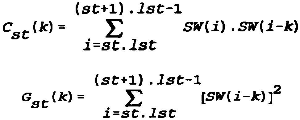
Les énergies par sous-trame R0 St sont également calculées
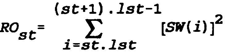
A l'étape 90, le module 36 détermine en outre, pour chaque sous-trame st, le retard entier Kst qui maximise l'estimation en boucle ouverte Pst Pst(k) du gain de prédiction à long terme sur la sous-trame st, en excluant les retards k pour lesquels l'autocorrélation Cst(k) est négative ou plus petite qu'une petite fraction de l'énergie Ru sot de la soustrame.L'estimation PSt(k) exprimée en décibels s'écrit Pst (k) = 20.log10[ROst/(ROst-CSt(k)/Gst(k))]
Maximiser St Pst(k) revient donc à maximiser l'expression
Xst (k) =Cst2 (k) /Gst (k) comme indiqué sur la figure 6. Le retard entier K St est le retard de base en résolution entière pour la sous-trame st. L'étape 90 est suivie par une comparaison 92 entre une première estimation en boucle ouverte du gain de prédiction global sur la trame courante et un seuil prédéterminé S0 typiquement compris entre 1 et 2 décibels (par exemple SO =1,5 dB). La première estimation du gain de prédiction global est égale à

où R0 est l'énergie totale de la trame (RO = R00+ R01+. .. + R0nst-1), et Xst(Kst)=Cst(Kst)/Gst (Kst) désigne le maximum déterminé à l'étape 90 relativement à la sous-trame st. comme l'indique la figure 6, la comparaison 92 peut être effectuée sans avoir à calculer le logarithme. In step 90, the module 36 further determines, for each subframe st, the integer delay Kst which maximizes the open-loop estimate Pst Pst (k) of the long-term prediction gain on the sub-frame st. , excluding the delays k for which the autocorrelation Cst (k) is negative or smaller than a small fraction of the energy Ru sot of the subtram. The estimate PSt (k) expressed in decibels is written Pst ( k) = 20.log10 [ROst / (ROst-CSt (k) / Gst (k))]
Maximize St Pst (k) is therefore to maximize the expression
Xst (k) = Cst2 (k) / Gst (k) as shown in Fig. 6. The integer delay K St is the full resolution base delay for the subframe st. Step 90 is followed by a comparison 92 between a first open loop estimate of the overall prediction gain on the current frame and a predetermined threshold S0 typically between 1 and 2 decibels (for example SO = 1.5 dB). The first estimate of the overall prediction gain is equal to
where R0 is the total energy of the frame (RO = R00 + R01 + ... + R0nst-1), and Xst (Kst) = Cst (Kst) / Gst (Kst) denotes the maximum determined in step 90 relative to the sub-frame st. as shown in FIG. 6, the comparison 92 can be performed without having to calculate the logarithm.
Si la comparaison 92 montre une première estimation du gain de prédiction inférieure au seuil S0, on considère que le signal de parole contient trop peu de corrélations à long terme pour être voisé, et le degré de voisement MV de la trame courante est pris égal à 0 à l'étape 94, ce qui termine dans ce cas les opérations effectuées par le module 36 sur cette trame. Si au contraire le seuil S0 est dépassé à l'étape 92, la trame courante est détectée comme voisée et le degré MV sera égal à 1, 2 ou 3. Le module 36 calcule alors, pour chaque sous-trame st, une liste Ist contenant des retards candidats pour constituer le centre ZP de l'intervalle de recherche des retards de prédiction à long terme. If the comparison 92 shows a first estimate of the prediction gain less than the threshold S0, it is considered that the speech signal contains too few long-term correlations to be voiced, and the voicing degree MV of the current frame is taken as equal to 0 in step 94, which ends in this case the operations performed by the module 36 on this frame. If instead the threshold S0 is exceeded in step 92, the current frame is detected as voiced and the degree MV will be equal to 1, 2 or 3. The module 36 then calculates, for each sub-frame st, a list Ist candidate delays to constitute the ZP center of the long-term prediction delay search interval.
Les opérations effectuées par le module 36 pour chaque sous-trame st (st initialisé à 0 à l'étape 96) d'une trame voisée commencent par la détermination 98 d'un seuil de sélection SE St en décibels égal à une fraction déterminée ss de l'estimation P5t(Kst) du gain de prédiction en décibels sur la sous-trame, maximisée à l'étape 90 (ss=0,75 typiquement) . Pour chaque sous-trame st d'une trame voisée, le module 36 détermine le retard de base rbf en résolution entière pour la suite du traitement. Ce retard de base pourrait être pris égal à l'entier Kst obtenu à l'étape 90. The operations performed by the module 36 for each subframe st (st initialized at 0 in step 96) of a voiced frame begin with the determination 98 of a selection threshold SE St in decibels equal to a determined fraction ss the estimate P5t (Kst) of the prediction gain in decibels on the subframe, maximized in step 90 (ss = 0.75 typically). For each subframe st of a voiced frame, the module 36 determines the basic delay rbf in full resolution for further processing. This base delay could be taken as equal to the integer Kst obtained in step 90.
Le fait de rechercher le retard de base en résolution fractionnaire autour de Kst permet toutefois de gagner en précision. L'étape 100 consiste ainsi, à rechercher, autour du retard entier Kst obtenu à l'étape 90, le retard fraction naire qui maximise l'expression CSt2/Gstv Cette recherche
St St peut être effectuée à la résolution maximale des retards fractionnaires (1/6 dans l'exemple décrit ici) même si le retard entier K St nest pas dans le domaine où cette résolution maximale s'applique.On détermine par exemple le nombre t qui maximise Cst2(Kst+6/6)/Gst(Kst+6/6) pour puis le retard de base rbf en résolution maximale est pris égal à KSt+ #st/6. Pour les valeurs fractionnaires T du retard, les autocorrélations st (T) et les énergies retardées Gst(T) sont obtenues par interpolation à partir des valeurs mémorisées à l'étape 90 pour les retards entiers. Bien entendu, le retard de base relatif à une sous-trame pourrait également être déterminé en résolution fractionnaire dès l'étape 90 et pris en compte dans la première estimation du gain de prédiction global sur la trame.Finding the base delay in fractional resolution around Kst, however, increases accuracy. Step 100 thus consists in searching, around the entire delay Kst obtained in step 90, the fractional delay which maximizes the expression CSt2 / Gstv.
St St can be performed at the maximum resolution of fractional delays (1/6 in the example described here) even if the entire delay K St is not in the domain where this maximum resolution applies. For example, the number t which maximizes Cst2 (Kst + 6/6) / Gst (Kst + 6/6) for then the base delay rbf in maximum resolution is taken equal to KSt + # st / 6. For the fractional values T of the delay, the autocorrelations st (T) and the delayed energies Gst (T) are obtained by interpolation from the values stored in step 90 for the entire delays. Of course, the base delay relative to a subframe could also be determined in fractional resolution from step 90 and taken into account in the first estimate of the overall prediction gain on the frame.
Une fois que le retard de base rbf a été déterminé pour une sous-trame, on procède à un examen 101 des sousmultiples de ce retard afin de retenir ceux pour lesquels le gain de prédiction est relativement important (figure 4), puis des multiples du plus petit sous-multiple retenu (figure 5). A l'étape 102, l'adresse j dans la liste Ist et l'index mdu sous-multiple sont initialisés à 0 et 1, respectivement. Once the basic delay rbf has been determined for a sub-frame, a sub-frame 101 examination is carried out of the delay to retain those for which the prediction gain is relatively large (Figure 4), then multiples of the sub-frame. smaller sub-multiple retained (Figure 5). In step 102, the address j in the list Ist and the index m of the submultiple are initialized to 0 and 1, respectively.
Une comparaison 104 est effectuée entre le sous-multiple rbf/m et le retard minimal rmin. Le sous-multiple rbf/m est à examiner s'il est supérieur à rmin. On prend alors pour l'entier i la valeur de l'index du retard quantifié ri le plus proche de rbf/m (étape 106), puis on compare, en 108, la valeur estimée du gain de prédiction Pst(ri) associée au retard quantifié ri pour la sous-trame considérée au seuil de sélection SE St calculé à l'étape 98
P5t(r) = 20.log10[ROst/[ROst- CSt2(r)/G5t(r))1 avec, pour les retards fractionnaires une interpolation des valeurs C St et G St calculées à l'étape 90 pour les retards entiers.Si St Pst(ri) < SEst, le retard ri n'est pas pris en considération, et on passe directement à l'étape 110 d'incrémentation de l'index m avant d'effectuer de nouveau la comparaison 104 pour le sous-multiple suivant. Si le test 108 montre que Pst(ri) # SEst, le retard ri est retenu et on exécute l'étape 112 avant d'incrémenter l'index m à l'étape 110. A l'étape 112, on mémorise l'index i à l'adresse j dans la liste Zist, on donne la valeur m à l'entier mO destiné à être égal à index du plus petit sous-multiple retenu, puis on incrémente dune unité adresse j.A comparison 104 is performed between the sub-multiple rbf / m and the minimum delay rmin. The sub-multiple rbf / m is to be examined if it is greater than rmin. We then take for the integer i the value of the index of the quantified delay ri closest to rbf / m (step 106), then compare, at 108, the estimated value of the prediction gain Pst (ri) associated with the quantized delay for the subframe considered at the selection threshold SE St calculated at step 98
P5t (r) = 20.log10 [ROst / [ROst-CSt2 (r) / G5t (r)) 1 with, for fractional delays, an interpolation of the values C St and G St calculated in step 90 for the whole delays If St Pst (ri) <SEst, the delay ri is not taken into consideration, and one goes directly to step 110 of incrementing the index m before making again the comparison 104 for the sub -Multiple next. If the test 108 shows that Pst (ri) # SEst, the delay ri is retained and step 112 is executed before incrementing the index m in step 110. In step 112, the index is memorized. i at the address j in the list Zist, we give the value m to the integer mO intended to be index equal to the smallest submultiplet retained, then we increment an address unit j.
L'examen des sous-multiples du retard de base est terminé lorsque la comparaison 104 montre rbf/m < rmin. On examine alors les retards multiples du plus petit rbf/m0 des sous-multiples précédemment retenus suivant le processus illustré sur la figure 5. Cet examen commence par une initialisation 114 de l'index n du multiple : n=2. Une comparaison 116 est effectuée entre le multiple n.rbf/m0 et le retard maximal rmax. Si n.rbf/m0 > rmax, on effectue le test 118 pour déterminer si 1' index mO du plus petit sous-multiple est un multiple entier de n. Dans l'affirmative, le retard n.rbf/mO a déjà été examiné lors de l'examen des sousmultiples de rbf, et on passe directement à l'étape 120 d'incrémentation de l'index n avant d'effectuer de nouveau la comparaison 116 pour le multiple suivant.Si le test 118 montre que mO n'est pas un multiple entier de n, le multiple n.rbf/m0 est à examiner. On prend alors pour l'entier i la valeur de l'index du retard quantifié ri le plus proche de n.rbf/m0 (étape 122), puis on compare, en 124, la valeur estimée du gain de prédiction Pst(ri) au seuil de sélection
SEst. Si st Pst(ri) < SEst, le retard ri n'est pas pris en consi- dération, et on passe directement à l'étape 120 d'incrémentation de l'index n. Si le test 124 montre que Pst(ri) 2 SESt, le retard ri est retenu et on exécute l'étape 126 avant d'incrémenter l'index n à l'étape 120. A l'étape 126, on mémorise l'index i à l'adresse j dans la liste ISt, puis on incrémente d'une unité l'adresse j.The sub-multiples examination of the basic delay is completed when the comparison 104 shows rbf / m <rmin. We then examine the multiple delays of the smallest rbf / m0 of the submultiples previously retained according to the process illustrated in FIG. 5. This examination begins with an initialization 114 of the index n of the multiple: n = 2. A comparison 116 is performed between the multiple n.rbf / m0 and the maximum delay rmax. If n.rbf / m0> rmax, the test 118 is performed to determine if the index mO of the smallest submultiple is an integer multiple of n. If yes, the delay n.rbf / mO has already been examined when examining the sub-multiples of rbf, and we go directly to step 120 of incrementing the index n before performing again the comparison 116 for the next multiple. If the test 118 shows that mO is not an integer multiple of n, the multiple n.rbf / m0 is to be examined. Then, for the integer i, we take the value of the index of the quantized delay ri closest to n.rbf / m0 (step 122), and then compare, at 124, the estimated value of the prediction gain Pst (ri) at the selection threshold
Its. If st Pst (ri) <SEst, the delay ri is not taken into consideration, and step 120 of incrementing the index n is directly entered. If the test 124 shows that Pst (ri) 2 SESt, the delay ri is retained and step 126 is executed before incrementing the index n in step 120. In step 126, the index is memorized. i at the address j in the list ISt, then we increment by one unit the address j.
L'examen des multiples du plus petit sous-multiple est terminé lorsque la comparaison 116 montre que n.rbf/m0 > rmax. A ce moment, la liste ISt contient j index de retards candidats. Si on souhaite limiter à jmax la longueur maximale de la liste Ist pour les étapes suivantes, on peut prendre la longueur ist de cette liste égale à min(j,jmax) (étape 128) puis, à l'étape 130, ordonner la liste ISt dans l'ordre des gains Cst(rIst(j))/Gst(rIst(j)) décroissants pour Osj < jst de façon à ne conserver que les ist retards procurant les plus grandes valeurs de gain.La valeur de jmax est choisie en fonction du compromis visé entre l'ef- ficacité de la recherche des retards LTP et la complexité de cette recherche. Des valeurs typiques de jmax vont de 3 à 5. The examination of the multiples of the smallest sub-multiple is completed when the comparison 116 shows that n.rbf / m0> rmax. At this time, the ISt list contains the index of candidate delays. If it is desired to limit the maximum length of the list Ist for the following steps to jmax, we can take the length ist of this list equal to min (j, jmax) (step 128) then, at step 130, order the list ISt in the order of gains Cst (rIst (j)) / Gst (rIst (j)) decreasing for Osj <jst so as to keep only the ist delays giving the largest gain values. The value of jmax is chosen depending on the trade-off between the effectiveness of the LTP delay search and the complexity of this research. Typical values of jmax range from 3 to 5.
Une fois que les sous-multiples et les multiples ont été examinés et que la liste 1St a ainsi été obtenue (figure 3), le module d'analyse 36 calcule une quantité Ymax déterminant une seconde estimation en boucle ouverte du gain de prédiction à long terme sur l'ensemble de la trame, ainsi que des index ZP, ZPO et ZP1 dans une phase 132 dont le déroulement est détaillé sur la figure 6. Cette phase 132 consiste à tester des intervalles de recherche de longueur N1 pour déterminer celui qui maximise une deuxième estimation du gain de prédiction global sur la trame. Les intervalles testés sont ceux dont les centres sont les retards candidats contenus dans la liste Ist calculée lors de la phase 101. La phase 132 commence par une étape 136 où l'adresse j dans la liste ISt est initialisée à 0. A l'étape 138, on vérifie si l'index ISt(j) a déjà été rencontré en testant un intervalle précédent centré sur Ist' (j') avec st' < st et 0j' < j5,, afin d'éviter de tester deux fois le même intervalle. Si le test 138 révèle que ISt(j) figurait déjà dans une liste Ist, avec st' < st, on incrémente directement l'adresse j à l'étape 140, puis on la compare à la longueur jst de la liste Zist. Si la comparaison 142 montre que j < jst, on revient à l'étape 138 pour la nouvelle valeur de l'adresse j.Lorsque la comparaison 142 montre que j=jst, tous les intervalles relatifs à la liste ISt ont été testés, et la phase 132 est terminée. Once sub-multiples and multiples have been examined and the list 1St has been obtained (FIG. 3), the analysis module 36 calculates a quantity Ymax determining a second open-loop estimation of the long-term prediction gain. term over the entire frame, as well as ZP, ZPO and ZP1 indexes in a phase 132 whose progress is detailed in Figure 6. This phase 132 is to test search intervals of length N1 to determine the one that maximizes a second estimate of the overall prediction gain on the frame. The intervals tested are those whose centers are the candidate delays contained in the list Ist calculated during the phase 101. The phase 132 begins with a step 136 where the address j in the list ISt is initialized to 0. At the step 138, we check whether the index ISt (j) has already been met by testing a previous interval centered on Ist '(j') with st '<st and 0j' <j5 ,, in order to avoid twice testing the same interval. If the test 138 reveals that ISt (j) was already in an Ist list, with st '<st, the address j is incremented directly at step 140, and then it is compared to the length jst of the list Zist. If the comparison 142 shows that j <jst, we return to step 138 for the new value of the address j.When the comparison 142 shows that j = jst, all the intervals relating to the list ISt have been tested, and phase 132 is completed.
Lorsque le test 138 est négatif, on teste l'intervalle centré sur Ist(j) en commençant par l'étape 148 où on détermine, pour chaque sous-trame st', l'index ist, du retard optimal qui maximise sur cet intervalle l'estimation en boucle ouverte Pst(ri) du gain de prédiction à long terme, cest-a- dire qui maximise la quantité Yst'(i)=Cst'(ri)/Gst'(ri) où ri désigne le retard quantifié d'index i pour Ist(j)-Nl/2 #i < Ist(j)+Nl/2 et osi < N. Lors de la maximisation 148 relative à une sous-trame st', on écarte a priori les index i pour lesquels l'autocorrélation Cst'(ri) est négative, pour éviter de dégrader le codage.S'il se trouve que toutes les valeurs de i comprises dans l'intervalle testé [I(j)-Nl/2, I(j)+Nl/2[ donnent lieu à des autocorrélations Cst,(ri) négatives, on sélectionne l'index ist' pour lequel cette autocorrélation est la plus petite en valeur absolue.When the test 138 is negative, the interval centered on Ist (j) is tested, starting with step 148 where, for each subframe st ', the index ist is determined of the optimal delay which maximizes over this interval. the open-loop estimation Pst (ri) of the long-term prediction gain, that is, that maximizes the quantity Yst '(i) = Cst' (ri) / Gst '(ri) where ri denotes the quantified delay index i for Ist (j) -Nl / 2 #i <Ist (j) + Nl / 2 and osi <N. When maximizing 148 relative to a subframe st ', a priori excludes the indexes i for which the autocorrelation Cst '(ri) is negative, to avoid degrading the coding.If it happens that all the values of i included in the tested interval [I (j) -Nl / 2, I (j ) + Nl / 2 [give rise to autocorrelations Cst, (ri) negative, the index ist 'is selected for which this autocorrelation is the smallest in absolute value.
Ensuite, en 150, la quantité Y déterminant la deuxième estimation du gain de prédiction global pour l'intervalle centré sur ISt(j) est calculée selon

puis comparée à Ymax, où Ymax représente la valeur à maximiser. Cette valeur Ymax est par exemple initialisée à
O en même temps que l'index st à l'étape 96. Si Y5Ymax, on passe directement à l'étape 140 d'incrémentation de l'index j. Si la comparaison 150 montre que Y > Ymax, on exécute l'étape 152 avant d'incrémenter l'adresse j à l'étape 140.Then, at 150, the quantity Y determining the second estimate of the overall prediction gain for the interval centered on ISt (j) is calculated according to
then compared to Ymax, where Ymax represents the value to be maximized. This value Ymax is for example initialized to
O at the same time as the index st in step 96. If Y5Ymax, go directly to step 140 of incrementing the index j. If the comparison 150 shows that Y> Ymax, step 152 is executed before incrementing the address j in step 140.
A cette étape 152, l'index ZP est pris égal à Ist(j) et les index ZPO et ZP1 sont respectivement pris égaux au plus petit et au plus grand des index ist déterminés à l'étape 148.At this step 152, the index ZP is taken equal to Ist (j) and the indexes ZPO and ZP1 are respectively equal to the smallest and largest of the indexes is determined in step 148.
A la fin de la phase 132 relative à une sous-trame st, l'index st est incrémenté d'une unité (étape 154) puis comparé, à l'étape 156, au nombre nst de sous-trames par trame. Si st < nst, on revient à l'étape 98 pour effectuer les opérations relatives à la sous-trame suivante. Lorsque la comparaison 156 montre que st=nst, l'index ZP désigne le centre de l'intervalle de recherche qui sera fourni au module 38 d'analyse LTP en boucle fermée, et ZPO et ZP1 sont des index dont l'écart est représentatif de la dispersion des retards optimaux par sous-trame dans 1' intervalle centré sur
ZP.At the end of the phase 132 relating to a subframe st, the index st is incremented by one unit (step 154) and then compared, in step 156, to the number nst of subframes per frame. If st <nst, we return to step 98 to perform the operations relating to the next sub-frame. When the comparison 156 shows that st = nst, the index ZP designates the center of the search interval that will be provided to the closed-loop LTP analysis module 38, and ZPO and ZP1 are indexes whose difference is representative. the dispersion of the optimal delays by subframe in the interval centered on
ZP.
A l'étape 158, le module 36 détermine le degré de voisement MV, sur la base de la seconde estimation en boucle ouverte du gain exprimée en décibels : Gp=20.1og10(RO/RO- Ymax). On fait appel à deux autres seuils S1 et S2. Si GpSS1, le degré de voisement MV est pris égal à 1 pour la trame courante. Le seuil S1 est typiquement compris entre 3 et 5 dB; par exemple 51=4 dB. Si Sl'=Gps2, le degré de voisement MV est pris égal à 2 pour la trame courante. Le seuil S2 est typiquement compris entre 5 et 8 dB ; par exemple S2=7 dB. Si
Gp > S2, on examine la dispersion des retards optimaux pour les différentes sous-trames de la trame courante.Si ZP1-ZP < N3/2 et ZP-ZPODN3/2, un intervalle de longueur N3 centré sur ZP suffit à prendre en compte tous les retards optimaux et le degré de voisement est pris égal à 3 (si Gp > S2). Sinon, si ZP1-ZP#N3/2 ou ZP-ZPO > N3/2, le degré de voisement est pris égal à 2 (si Gp > S2). In step 158, the module 36 determines the degree of voicing MV, based on the second open-loop estimation of the gain expressed in decibels: Gp = 20.1og10 (RO / RO-Ymax). Two other thresholds S1 and S2 are used. If GpSS1, the degree of voicing MV is taken equal to 1 for the current frame. The threshold S1 is typically between 3 and 5 dB; for example 51 = 4 dB. If Sl '= Gps2, the degree of voicing MV is taken as 2 for the current frame. The threshold S2 is typically between 5 and 8 dB; for example S2 = 7 dB. Yes
Gp> S2, we examine the dispersion of the optimal delays for the different subframes of the current frame.If ZP1-ZP <N3 / 2 and ZP-ZPODN3 / 2, an interval of length N3 centered on ZP is sufficient to take into account all the optimal delays and the degree of voicing is taken equal to 3 (if Gp> S2). Otherwise, if ZP1-ZP # N3 / 2 or ZP-ZPO> N3 / 2, the degree of voicing is taken as 2 (if Gp> S2).
L'index ZP du centre de l'intervalle de recherche du retard de prédiction pour une trame voisée peut être compris entre 0 et N-1=255, et l'index différentiel DP déterminé pour le module 38 peut aller de -16 à +15 si MV=1 ou 2, et de -8 à +7 si MV=3 (cas N1=32, N3=16). L'index ZP+DP du retard TP finalement déterminé peut donc dans certains cas être plus petit que 0 ou plus grand que 255. Ceci permet à l'analyse
LTP en boucle fermée de porter également sur quelques retards
TP plus petits que rmin ou plus grands que rmax. On améliore ainsi la qualité subjective de la restitution des voix dites pathologiques et des signaux non vocaux (fréquences vocales
DTMF ou fréquences de signalisation utilisées par le réseau téléphonique commuté).Une autre possibilité est de prendre pour l'intervalle de recherche les 32 premiers ou derniers index de quantification des retards si ZP < 16 ou ZP > 240 avec
MV=1 ou 2, et les 16 premiers ou derniers index si ZP < 8 ou ZP > 248 avec MV=3.The center ZP index of the prediction delay search interval for a voiced frame can be between 0 and N-1 = 255, and the differential index DP determined for the module 38 can range from -16 to + 15 if MV = 1 or 2, and from -8 to +7 if MV = 3 (case N1 = 32, N3 = 16). The index ZP + DP of the delay TP finally determined can therefore in some cases be smaller than 0 or greater than 255. This allows the analysis
LTP closed loop to also carry on some delays
TP smaller than rmin or larger than rmax. This improves the subjective quality of the restitution of so-called pathological voices and non-vocal signals (vocal frequencies
DTMF or signaling frequencies used by the switched telephone network). Another possibility is to take for the search interval the first 32 or last quantization indexes of delays if ZP <16 or ZP> 240 with
MV = 1 or 2, and the first 16 or last indexes if ZP <8 or ZP> 248 with MV = 3.
Le fait de réduire l'intervalle de recherche des retards pour les trames très voisées (typiquement 16 valeurs pour MV=3 au lieu de 32 pour MV=1 ou 2) permet de diminuer la complexité de 1 'analyse LTP en boucle fermée effectuée par le module 38 en réduisant le nombre de convolutions yT(i) à calculer suivant la formule (1). Un autre avantage est qu'un bit de codage de l'index différentiel DP est économisé. Le débit de sortie étant constant, ce bit peut être réalloué au codage d'autres paramètres. On peut en particulier allouer ce bit supplémentaire à la quantification du gain de prédiction à long terme gp calculé par le module 40. En effet, une meilleure précision sur le gain gp grâce à un bit de quantification supplémentaire est appréciable car ce paramètre est perceptuellement important pour les sous-trames très voisées (MV=3). Une autre possibilité est de prévoir un bit de parité pour le retard TP et/ou le gain gp, permettant de détecter d'éventuelles erreurs affectant ces paramètres. Reducing the delay search interval for highly voiced frames (typically 16 values for MV = 3 instead of 32 for MV = 1 or 2) reduces the complexity of the closed-loop LTP analysis performed by the module 38 by reducing the number of convolutions yT (i) to be calculated according to formula (1). Another advantage is that a coding bit of the differential index DP is saved. Since the output rate is constant, this bit can be reallocated to the encoding of other parameters. In particular, this extra bit can be allocated to the quantization of the long-term prediction gain gp calculated by the module 40. Indeed, a better accuracy on the gain gp by virtue of an additional quantization bit is appreciable because this parameter is perceptually important. for very voiced subframes (MV = 3). Another possibility is to provide a parity bit for the delay TP and / or the gain gp, making it possible to detect any errors affecting these parameters.
Il est possible d'apporter quelques modifications au processus d'analyse LTP en boucle ouverte décrit ci-dessus en référence aux figures 3 à 6. It is possible to make some modifications to the open-loop LTP analysis process described above with reference to FIGS. 3-6.
Suivant une première variante de ce processus, les premières optimisations effectuées à l'étape 90 relativement aux différentes sous-trames sont remplacées par une seule optimisation portant sur l'ensemble de la trame. Outre les paramètres Cet (ka et GSt(k) calculés pour chaque sous-trame st, on calcule également les autocorrélations C(k) et les énergies retardées G(k) pour l'ensemble de la trame

On détermine alors le retard de base en résolution entière K qui maximise X(k)=C2(k)/G(k) pour rmin s k s rmax. We then determine the basic delay in integer resolution K which maximizes X (k) = C2 (k) / G (k) for rmin s k s rmax.
La première estimation du gain comparée à 50 à l'étape 92 est alors P(K)=20.log10 [RO/ [RO-X(K)] ]. On détermine ensuite, autour de K, un seul retard de base en résolution fractionnaire rbf et l'examen 101 des sous-multiples et des multiples est effectué une seule fois et produit une seule liste I au lieu de nst listes ISt. La phase 132 est ensuite effectuée une seule fois pour cette liste I, en ne distinguant les soustrames qu'aux étapes 148, 150 et 152. Cette variante de réalisation a pour avantage de réduire la complexité de l'analyse en boucle ouverte.The first estimate of the gain compared to 50 in step 92 is then P (K) = 20.log10 [RO / [RO-X (K)]]. Then, around K, a single base delay is determined in fractional resolution rbf and the examination 101 of the submultiples and multiples is done once and produces a single list I instead of nst lists ISt. Phase 132 is then performed once for this list I, only distinguishing the subframes in steps 148, 150 and 152. This embodiment has the advantage of reducing the complexity of open loop analysis.
Suivant une seconde variante du processus d'analyse
LTP en boucle ouverte, le domaine [rmin, rmax] des retards possibles est subdivisé en nz sous-intervalles ayant par exemple la même longueur (nz=3 typiquement), et les premières optimisations effectuées à 1 'étape 90 relativement aux différentes sous-trames sont remplacées par nz optimisations dans les différents sous-intervalles portant chacune sur l'ensemble de la trame. On obtient ainsi nz retards de base
K1 t Knz en résolution entière. La décision voisé/non voisé (étape 92) est prise sur la base de celui des retards de base Ki qui procure la plus grande valeur pour la première estimation en boucle ouverte du gain de prédiction à long terme.Ensuite, si la trame est voisée, on détermine les retards de base en résolution fractionnaire par le même processus qu'à l'étape 100, mais en autorisant seulement les valeurs de retard quantifiées. L'examen 101 des sousmultiples et des multiples n'est pas effectué. Pour la phase 132 de calcul de la seconde estimation du gain de prédiction, on prend comme retards candidats les nz retards de base précédemment déterminés. Cette seconde variante permet de se dispenser de l'examen systématique des sous-multiples et des multiples qui sont en général pris en considération grace à la subdivision du domaine des retards possibles.According to a second variant of the analysis process
LTP open loop, the domain [rmin, rmax] possible delays is subdivided into nz subintervals having, for example, the same length (nz = 3 typically), and the first optimizations carried out at step 90 relative to the different sub-intervals. Frames are replaced by nz optimizations in the different sub-intervals each bearing on the whole of the frame. We thus obtain nz basic delays
K1 t Knz in full resolution. The voiced / unvoiced decision (step 92) is made on the basis of that of the base delays Ki which provides the greatest value for the first open-loop estimation of the long-term prediction gain. Then, if the frame is voiced the basic delays in fractional resolution are determined by the same process as in step 100, but allowing only the quantized delay values. Exam 101 of sub-multiples and multiples is not performed. For the calculation phase 132 of the second estimation of the prediction gain, the initial delays n.sub.1 are determined as candidate delays. This second variant makes it possible to dispense with the systematic examination of submultiples and multiples which are generally taken into account by subdividing the domain of possible delays.
Suivant une troisième variante du processus d'analyse
LTP en boucle ouverte, la phase 132 est modifiée en ce que, aux étapes d'optimisation 148, on détermine d'une part l'index ist, qui maximise Cst'(ri)/Gst'(ri) pour Ist(j)N1/2si < Ist(j)+N1/2 et Osi < N, et d'autre part, au cours de la même boucle de maximisation, l'index kst' qui maximise cette même quantité sur un intervalle réduit
Ist(i)-N3/25i < Ist(i)+N3/2 et O Osi < N. L'étape 152 est également modifiée : on ne mémorise plus les index ZPO et
ZP1, mais une quantité Ymax' définie de la même manière que
Ymax mais en référence à l'intervalle de longueur réduite

LTP in an open loop, the phase 132 is modified in that, at the optimization steps 148, the index ist is determined on the one hand, which maximizes Cst '(ri) / Gst' (ri) for Ist (j) N1 / 2si <Ist (j) + N1 / 2 and Osi <N, and on the other hand, during the same maximization loop, the index kst 'which maximizes this same quantity over a reduced interval
Ist (i) -N3 / 25i <Ist (i) + N3 / 2 and O Osi <N. Step 152 is also modified: the ZPO indexes are no longer stored and
ZP1, but a quantity Ymax 'defined in the same way as
Ymax but with reference to the reduced length interval
Dans cette troisième variante, la détermination 158 du mode de voisement conduit à sélectionner plus souvent le degré de voisement MV=3.On prend également en compte, en plus du gain Gp précédemment décrit, une troisième estimation en boucle ouverte du gain LTP, correspondant à Ymax'
Gp'=20.log10[RO/(RO-Ymax')]. Le degré de voisement est MV=1 si GpSSl, MV=3 si Gp' > S2 et MV=2 si aucune de ces deux conditions n'est vérifiée. En augmentant ainsi la proportion de trames de degré MV=3, on réduit la complexité moyenne de l'analyse en boucle fermée et on améliore la robustesse aux erreurs de transmission.In this third variant, the determination 158 of the voicing mode leads to selecting the degree of voicing MV = 3 more often. In addition to the gain Gp previously described, a third open loop estimate of the corresponding LTP gain is also taken into account. at Ymax '
Gp = 20.log10 [RO / (RO-Ymax ')]. The degree of voicing is MV = 1 if GpSSl, MV = 3 if Gp '> S2 and MV = 2 if neither of these two conditions are satisfied. By thus increasing the proportion of frames of degree MV = 3, the average complexity of the closed-loop analysis is reduced and the robustness to transmission errors is improved.
Une quatrième variante du processus d'analyse LTP en boucle ouverte concerne surtout les trames faiblement voisées (MV=1). Ces trames correspondent souvent à un début ou à une fin d'une zone de voisement. Fréquemment, ces trames peuvent comporter de une à trois sous-trames pour lesquelles le coefficcient de gain du filtre de synthèse à long terme est nul voire négatif. Il est proposé de ne pas effectuer l'analyse
LTP en boucle fermée pour les sous-trames en question, afin de réduire la complexité moyenne du codage. Ceci peut être réalisé en mémorisant à l'étape 152 de la figure 6 nst pointeurs indiquant pour chaque sous-trame st' si l'autocorréla- tion Cst. correspondant au retard d'index ist. est négative ou encore très petite.Une fois que tous les intervalles référencés dans les listes Zist, les sous-trames pour lesquelles le gain de prédiction est négatif ou négligeable peuvent être identifiées en consultant les nst pointeurs. Le cas échéant le module 38 est désactivé pour les sous-trames correspondantes. Ceci n'affecte pas la qualité de l'analyse LTP puisque le gain de prédiction correspondant à ces sous-trames sera de toutes façons quasiment nul.A fourth variant of the open-loop LTP analysis process concerns mainly weakly voiced frames (MV = 1). These frames often correspond to a beginning or end of a voicing area. Frequently, these frames may comprise from one to three sub-frames for which the gain coefficient of the long-term synthesis filter is zero or even negative. It is proposed not to carry out the analysis
Closed-loop LTPs for the sub-frames in question, to reduce the average complexity of the coding. This can be done by storing in step 152 of FIG. 6 nst pointers indicating for each sub-frame st 'whether the autocorrelation Cst. corresponding to the index delay ist. is negative or very small.Once all the intervals referenced in the Zist lists, the subframes for which the prediction gain is negative or negligible can be identified by consulting the nst pointers. If necessary, the module 38 is deactivated for the corresponding sub-frames. This does not affect the quality of the LTP analysis since the prediction gain corresponding to these subframes will in any case be almost zero.
Un autre aspect de l'invention concerne le module 42 de calcul de la réponse impulsionnelle du filtre de synthèse pondéré. Le module 38 d'analyse LTP en boucle fermée a besoin de cette réponse impulsionnelle h sur la durée d'une soustrame pour calculer les convolutions yT(i) selon la formule (1). Le module 40 d'analyse stochastique en a également besoin pour calculer des convolutions comme on le verra plus loin. Le fait d'avoir à calculer des convolutions avec une réponse h s'étendant sur la durée d'une sous-trame (lst=40 typiquement) implique une relative complexité du codage, qu' il serait souhaitable de réduire notamment pour augmenter l'autonomie de la station mobile. Dans certains cas il a été proposé de tronquer la réponse impulsionnelle à une longueur inférieure à la longueur d'une sous-trame (par exemple à 20 échantillons), mais ceci peut dégrader la qualité du codage. Another aspect of the invention relates to the module 42 for calculating the impulse response of the weighted synthesis filter. The closed-loop LTP analysis module 38 needs this impulse response h over the duration of a subframe to calculate the convolutions yT (i) according to formula (1). The stochastic analysis module 40 also needs it to calculate convolutions as will be seen later. The fact of having to compute convolutions with a response h extending over the duration of a sub-frame (typically lst = 40) implies a relative complexity of the coding, which it would be desirable to reduce in particular to increase the autonomy of the mobile station. In some cases it has been proposed to truncate the impulse response to a length less than the length of a subframe (for example 20 samples), but this can degrade the quality of the coding.
On propose selon l'invention de tronquer la réponse impulsionnelle h en tenant compte d'une part de la distribution énergétique de cette réponse et d'autre part du degré de voi sement MV de la trame considérée, déterminé par le module 36 d'analyse LTP en boucle ouverte.According to the invention, it is proposed to truncate the impulse response h while taking into account, on the one hand, the energy distribution of this response and, on the other hand, the degree of MV value of the frame considered, determined by the analysis module 36. LTP in open loop.
Les opérations effectuées par le module 42 sont par exemple conformes à l'organigramme de la figure 7. La réponse impulsionnelle est d'abord calculée à l'étape 160 sur une longueur pst supérieure à la longueur d'une sous-trame et suffisamment grande pour qu'on soit assuré de prendre en compte toute l'énergie de la réponse impulsionnelle (par exemple pst=60 pour nst=4 et lst=40 si la prédiction linéaire à court terme est d'ordre q=10).A l'étape 160, on calcule également les énergies tronquées de la réponse impulsionnelle :

Les composantes h(i > de la réponse impulsionnelle et les énergies tronquées Eh(i) peuvent être obtenues en filtrant une impulsion unitaire au moyen d'un filtre de fonction de transfert W(z)tA(z) d'états initiaux nuls, ou encore par récurrence

Eh(i) = Eh Eh(i-1) + (h < I) J2 pour O < i < pst, avec f(i)=h(i)=0 pour i < O, 8(0)=f(0)=h(0)=Eh(0 ) =1, et 8(i)=O pour i*O. Dans l'expression (2), les coefficients ak sont ceux intervenant dans le filtre de pondération perceptuelle, c'est-à-dire les coefficients de prédiction linéaire interpolés mais non quantifiés, tandis que dans l'expression (3), les coefficients ak sont ceux appliqués au filtre de synthèse, c'est-à-dire les coefficients de prédiction linéaire quantifiés et interpolés. Eh (i) = Eh Eh (i-1) + (h <I) J2 for O <i <pst, with f (i) = h (i) = 0 for i <O, 8 (0) = f ( 0) = h (0) = Eh (0) = 1, and 8 (i) = O for i * O. In expression (2), the coefficients ak are those involved in the perceptual weighting filter, ie the interpolated but unquantized linear prediction coefficients, while in the expression (3), the coefficients ak are those applied to the synthesis filter, that is to say the quantized and interpolated linear prediction coefficients.
Ensuite le module 42 détermine la plus petite longueur La telle que l'énergie Eh(La-l) de la réponse impul sionnelle tronquée à La échantillons soit au moins égale à une proportion a de son énergie totale Eh(pst-l) estimée sur pst échantillons. Une valeur typique de a est 98%. Le nombre
La est initialisé à pst à l'étape 162 et décrémenté d'une unité en 166 tant que Eh(L -2) > avEh(pst-l) (test 164). La longueur La cherchée est obtenue lorsque le test 164 montre que Eh(Lα-2)#α.Eh(pst-1). Then the module 42 determines the shortest length La such that the energy Eh (La-1) of the impulse response truncated to the samples is at least equal to a proportion a of its total energy Eh (pst-1) estimated on pst samples. A typical value of a is 98%. The number
La is initialized to pst at step 162 and decremented by one unit at 166 as Eh (L -2)> avEh (pst-1) (test 164). The length The sought is obtained when the test 164 shows that Eh (L α -2) # α .Eh (pst-1).
Pour tenir compte du degré de voisement Mv, un terme correcteur A(MV) est ajouté à la valeur de La qui a été obtenue (étape 168). Ce terme correcteur est de préférence une fonction croissante du degré de voisement. On peut par exemple prendre A < 0)=-5, #(1)=0, #(2)=+5 et A(3)=+7. De cette façon, la réponse impulsionnelle h sera déterminée de façon d'autant plus précise que le voisement de la parole est important. La longueur de troncature Lh de la réponse impulsionnelle est prise égale à La si Lauist et à nst sinon. Les échantillons restants de la réponse impulsionnelle (h(i)=O avec i2Lh) peuvent être annulés. To account for the voicing degree Mv, a correction term A (MV) is added to the value of La which has been obtained (step 168). This correcting term is preferably an increasing function of the degree of voicing. For example, we can take A <0) = - 5, # (1) = 0, # (2) = + 5 and A (3) = + 7. In this way, the impulse response h will be determined more precisely as the voicing of speech is important. The truncation length Lh of the impulse response is taken equal to La if Lauist and to nst otherwise. The remaining samples of the impulse response (h (i) = O with i2Lh) can be canceled.
Avec la troncature de la réponse impulsionnelle, le calcul (1) des convolutions yT(i) par le module 38 d'analyse
LTP en boucle fermée est modifié de la façon suivante :

LTP in closed loop is modified as follows:
L'obtention de ces convolutions, qui représente une part importante des calculs effectués, nécessite donc sensiblement moins de multiplications, d'additions et d'adressages dans le répertoire adaptatif lorsque la réponse impulsionnelle est tronquée. La troncature dynamique de la réponse impulsionnelle faisant intervenir le degré de voisement MV permet d'obtenir une telle réduction de complexité sans affecter la qualité du codage. Les mêmes considérations s'appliquent pour les calculs de convolutions effectués par le module 40 d'analyse stochastique.Ces avantages sont parti-culièrement appréciables lorsque le filtre de pondération perceptuelle a une-fonction de transfert de la forme W(z)=A(z/Tl)/A(z/Y2) avec 0 < Y2 < Y1 < 1 qui donne lieu à des réponses impulsionnelles généralement plus longues que celles de la forme
W(z)=A(z)/A(z/Y) plus communément employées dans les codeurs à analyse par synthèse.Obtaining these convolutions, which represents an important part of the calculations performed, therefore requires substantially fewer multiplications, additions and addresses in the adaptive directory when the impulse response is truncated. The dynamic truncation of the impulse response using the voicing degree MV makes it possible to obtain such a reduction in complexity without affecting the quality of the coding. The same considerations apply to the convolution calculations performed by the stochastic analysis module 40. These advantages are particularly appreciable when the perceptual weighting filter has a transfer function of the form W (z) = A ( z / Tl) / A (z / Y2) with 0 <Y2 <Y1 <1 which gives rise to impulse responses generally longer than those of the form
W (z) = A (z) / A (z / Y) more commonly used in synthetic analysis coders.
Un troisième aspect de l'invention concerne le module 40 d'analyse stochastique servant à modéliser la partie non prédictible de l'excitation. A third aspect of the invention relates to the stochastic analysis module 40 for modeling the unpredictable portion of the excitation.
L'excitation stochastique considérée ici est de type multi-impulsionnelle. L'excitation stochastique relative à une sous-trame est représentée par np impulsions de positions p(n) et d'amplitudes, ou gains, g(n) (lsnsnp). Le gain gp de prédiction à long terme peut également être calculé au cours du même processus. De façon générale, on peut considérer que la séquence d'excitation relative à une sous-trame comporte nc contributions associées respectivement à nc gains. Les contributions sont des vecteurs lst échantillons qui, pondérés par les gains associés et sommés correspondent à la séquence d'excitation du filtre de synthèse à court terme. The stochastic excitation considered here is of the multi-pulse type. The stochastic excitation relative to a sub-frame is represented by np pulses of positions p (n) and amplitudes, or gains, g (n) (lsnsnp). The long-term prediction gp gain can also be calculated during the same process. In general terms, it can be considered that the excitation sequence relating to a sub-frame comprises nc contributions associated respectively with nc gains. The contributions are lst sample vectors which, weighted by the associated and summed gains, correspond to the excitation sequence of the short-term synthesis filter.
Une des contributions peut être prédictible, ou plusieurs dans le cas d'un filtre de synthèse à long terme à plusieurs prises ("multi-tap pitch synthesis filtrer"). Les autres contributions sont dans le cas présent np vecteurs ne comportant que des O sauf une impulsion d'amplitude 1. On a donc nc=np si MV=O, et nc=np+l si MV=1, 2 ou 3.One of the contributions can be predictable, or several in the case of a long-term multi-tap synthesis filter ("multi-tap pitch synthesis"). The other contributions are in this case np vectors containing only O except a pulse of amplitude 1. We thus have nc = np if MV = O, and nc = np + l if MV = 1, 2 or 3.
L'analyse multi-impulsionnelle incluant le calcul du gain gp=gZO) consiste, de façon connue, à trouver pour chaque sous-trame des positions p(n) (lsnsnp) et des gains g(n) (Onnp) qui minimisent l'erreur quadratique pondérée perceptuellement E entre le signal de parole et le signal synthétisé, donnée par :

les gains étant solution du système linéaire g.B=b.The multi-pulse analysis including the calculation of the gain gp = gZO) consists, in known manner, of finding for each sub-frame positions p (n) (lsnsnp) and gains g (n) (Onnp) which minimize the perceptually weighted squared error E between the speech signal and the synthesized signal, given by:
the gains being solution of the linear system gB = b.
Dans les notations ci-dessus
- x désigne un vecteur-cible initial composé des lst échantillons du signal de parole pondéré SW sans mémoire x=(x(0),x(l),..., x(lst-l) ), les x(i) ayant été calculés comme indiqué précédemment lors de l'analyse LTP en boucle fermée
- g désigne le vecteur ligne composé des np+1 gains g=(g(O)=gpR g(l),...,g(np)) ;
- les vecteurs-ligne Fp(n > (0#n < nc) sont des contributions pondérées ayant pour composantes i(0#i < lst) les produits de convolution entre la contribution n à la séquence d'excitation et la réponse impulsionnelle h du filtre de synthèse pondéré
- b désigne le vecteur ligne composé des nc produits scalaires entre le vecteur X et les vecteurs ligne Fp(n);;
- B désigne une matrice symétrique à nc lignes et nc colonnes dont le terme Bi,j=Fp(i).Fp(j)T (0#i,j < nc) est égal au produit scalaire entre les vecteurs Fp(i) et Fp < j) précédemment définis
- (.)T désigne la transposition matricielle.In the notations above
x denotes an initial target vector composed of lst samples of the weighted speech signal SW without memory x = (x (0), x (l), ..., x (lst-1)), the x (i) having been calculated as indicated previously during closed loop LTP analysis
- g denotes the line vector composed of np + 1 gains g = (g (O) = gpR g (1), ..., g (np));
the line vectors Fp (n> (0 # n <nc) are weighted contributions having as components i (0 # i <lst) the products of convolution between the contribution n to the excitation sequence and the impulse response h weighted synthesis filter
b denotes the line vector composed of nc scalar products between the vector X and the line vectors Fp (n);
B denotes a symmetric matrix with nc rows and nc columns whose term Bi, j = Fp (i) .Fp (j) T (0 # i, j <nc) is equal to the dot product between the vectors Fp (i) and Fp <j) previously defined
- (.) T denotes the matrix transposition.
Pour les impulsions de l'excitation stochastique (1#n Snp=nc-l) les vecteurs Fp(n) sont simplement constitués par le vecteur de la réponse impulsionnelle h décalée de p(n) échantillons. Le fait de tronquer la réponse impulsionnelle comme décrit précédemment permet donc de réduire sensiblement le nombre d'opérations utiles au calcul des produits scalaires faisant intervenir ces vecteurs Fp(n). Pour la contribution prédictible de l'excitation, le vecteur Fp(o)=YTp a pour composantes Fp(0)(i) (0#i < lst) les convolutions yTP(i) que le module 38 a calculées suivant la formule (1) ou (1') pour le retard de prédiction à long terme sélectionné TP. Si MV=O, la contribution n=O est également de type impulsion nelle et la position p(O) est à calculer. For the pulses of the stochastic excitation (1 # n Snp = nc-1) the vectors Fp (n) are simply constituted by the vector of the impulse response h shifted by p (n) samples. Truncating the impulse response as described above thus makes it possible to substantially reduce the number of operations that are useful for calculating scalar products using these vectors Fp (n). For the predictable contribution of the excitation, the vector Fp (o) = YTp has for components Fp (0) (i) (0 # i <lst) the convolutions yTP (i) that the modulus 38 has calculated according to the formula ( 1) or (1 ') for the selected long-term prediction delay TP. If MV = O, the contribution n = O is also of the impulse type and the position p (O) is to be calculated.
Minimiser l'erreur quadratique E définie ci-dessus revient à trouver l'ensemble des positions p(n) qui maximisent la corrélation normalisée b.B 1.bT puis à calculer les gains selon g=b.B-1. Minimizing the squared error E defined above amounts to finding all the positions p (n) which maximize the normalized correlation b.B 1.bT and then calculating the gains according to g = b.B-1.
Mais une recherche exhaustive des positions d'impulsion nécessiterait un volume de calculs excessif. Pour atténuer ce problème, l'approche multi-impulsionnelle applique en général une procédure sous-optimale consistant à calculer successivement les gains et/ou les positions d'impulsion pour chaque contribution.Pour chaque contribution n (0#n < nc), on détermine d'abord la position p(n) qui maximise la corrélation normalisée (F.e1T)2/(F. FpT), on recalcule les gains gn(0) à g n gn(n) selon gn=bn.Bn 1, où n=(gn(0),...,gn(n)), bn=(b(0),...,b(n)) et Bn={Bi,j}0#i,j#n, puis on calcule pour l'itération suivante le vecteur-cible en égal au vecteur-cible initial X auquel on retranche les contributions 0 à n du signal synthétique pondéré multipliées par leurs gains respectifs

A l'issue de la dernière itération nc-l, les gains gnc-1(i) sont les gains sélectionnés et l'erreur quadratique minimisée E est égal à l'énergie du vecteur-cible enC-l
La méthode ci-dessus donne des résultats satisfaisants, mais elle nécessite l'inversion d'une matrice B n à chaque itération. Dans leur article "Amplitude Optimization and Pitch Prediction in Multipulse Codera (IEEE Trans. on
Acoustics, Speech, and Signal Processing, Vol.37, N 3, Mars 1989, pages 317-327), S. Singhal et B.S. Atal ont proposé de simplifier le problème de l'inversion des matrices Bn en utilisant la décomposition de Cholesky : B -M M T Mn est une matrice triangulaire inférieure. Cette décomposition est possible parce que Bn est une matrice symétrique à valeurs propres positives. L'avantage de cette approche est que l'inversion d'une matrice triangulaire est relativement peu complexe, Bn-l pouvant être obtenue par Bn-1=(Mn-1)T.Mn-1 .At the end of the last iteration nc-1, the gains gnc-1 (i) are the selected gains and the minimized quadratic error E is equal to the energy of the target vector enC-1
The above method gives satisfactory results, but it requires the inversion of a matrix B n at each iteration. In their article "Amplitude Optimization and Pitch Prediction in Multipulse Codera (IEEE Trans.
Acoustics, Speech, and Signal Processing, Vol.37, No. 3, March 1989, pages 317-327), S. Singhal and BS Atal proposed to simplify the problem of inverting Bn matrices using Cholesky decomposition: B -MMT Mn is a lower triangular matrix. This decomposition is possible because Bn is a symmetric matrix with positive eigenvalues. The advantage of this approach is that the inversion of a triangular matrix is relatively uncomplicated, Bn-1 can be obtained by Bn-1 = (Mn-1) T.Mn-1.
La décomposition de Cholesky et l'inversion de la matrice Mn nécessitent toutefois d'effectuer des divisions et des calculs de racines carrées qui sont des opérations exigentes en termes de complexité de calcul. L'invention propose de simplifier considérablement la mise en oeuvre de l'optimisation en modifiant la décomposition des matrices Bn de la façon suivante :
Bn = Ln.RnT = (Ln.(Ln.Kn-1)T où Kn est une matrice diagonale et Ln est une matrice triangulaire inférieure n'ayant que des 1 sur sa diagonale principale (soit Ln=Mn.Kn1/2 avec les notations précédentes).The decomposition of Cholesky and the inversion of the matrix Mn, however, require division and square root calculations which are operations that are demanding in terms of calculation complexity. The invention proposes to considerably simplify the implementation of optimization by modifying the decomposition of matrices Bn as follows:
Bn = Ln.RnT = (Ln. (Ln.Kn-1) T where Kn is a diagonal matrix and Ln is a lower triangular matrix having only 1 on its main diagonal (ie Ln = Mn.Kn1 / 2 with previous notations).
Compte-tenu de la structure de la matrice Bn, les matrices
Ln=Bn.Kn, Rn Kfl et Ln 1 sont construites chacune par simple adjonction d'une ligne aux matrices correspondantes de l'itération précédente :

Ln = Bn.Kn, Rn Kfl and Ln 1 are each constructed by simply adding a line to the corresponding matrices of the previous iteration:
<tb> <SEP> t <SEP> B(n,O) <SEP> o <SEP>
<tb> <SEP> Bn <SEP> = <SEP> # <SEP> Bn-1 <SEP> # <SEP> Ln <SEP> = <SEP> # <SEP> Ln-1 <SEP> . <SEP> #
<tb> <SEP> B(n,n1) <SEP> 0 <SEP>
<tb> <SEP> B(n,O) <SEP> . <SEP> . <SEP> . <SEP> B(n,n-1) <SEP> B(n,n) <SEP> I <SEP> L(n,O) <SEP> . <SEP> . <SEP> .<SEP> L(n,n-1) <SEP> I
<tb> <SEP> k <SEP>
<tb> <SEP> 0 <SEP> o <SEP>
<tb> <SEP> Rn <SEP> = <SEP> # <SEP> Rn-1 <SEP> # <SEP> Kn <SEP> = <SEP> # <SEP> . <SEP> #
<tb> <SEP> 0 <SEP> 0
<tb> R(n,O) <SEP> . <SEP> . <SEP> R(n,n-i) <SEP> R(n,n) <SEP> 0 <SEP> . <SEP> . <SEP> 0 <SEP> K(n) <SEP>
<tb> <SEP> o <SEP>
<tb> yl <SEP> Ln-i <SEP> -1
<tb> o <SEP>
<tb> <SEP> #L-1(n,0) <SEP> . <SEP> . <SEP> .<SEP> L-1(n,n-1) <SEP> 1#
<tb>
Dans ces conditions, la décomposition de Bn, l'inversion de Ln l'obtention de Bn-1=Kn.(Ln-1)T.Ln-1 et le recalcul des gains ne nécessitent qu'une seule division par itération et aucun calcul de racine carrée.<tb><SEP> t <SEP> B (n, O) <SEP> o <SEP>
<tb><SEP> Bn <SEP> = <SEP>#<SEP> Bn-1 <SEP>#<SEP> Ln <SEP> = <SEP>#<SEP> Ln-1 <SEP>. <SEP>#
<tb><SEP> B (n, n1) <SEP> 0 <SEP>
<tb><SEP> B (n, O) <SEP>. <SEP>. <SEP>. <SEP> B (n, n-1) <SEP> B (n, n) <SEP> I <SEP> L (n, O) <SEP>. <SEP>. <SEP>. <SEP> L (n, n-1) <SEP> I
<tb><SEP> k <SEP>
<tb><SEP> 0 <SEP> o <SEP>
<tb><SEP> Rn <SEP> = <SEP>#<SEP> Rn-1 <SEP>#<SEP> Kn <SEP> = <SEP>#<SEP>.<SEP>#
<tb><SEP> 0 <SEP> 0
<tb> R (n, O) <SEP>. <SEP>. <SEP> R (n, n) <SEP> R (n, n) <SEP> 0 <SEP>. <SEP>. <SEP> 0 <SEP> K (n) <SEP>
<tb><SEP> o <SEP>
<tb> yl <SEP> Ln-i <SEP> -1
<tb> o <SEP>
<tb><SEP># L-1 (n, 0) <SEP>. <SEP>. <SEP>. <SEP> L-1 (n, n-1) <SEP> 1 #
<Tb>
Under these conditions, the decomposition of Bn, the inversion of Ln, the obtaining of Bn-1 = Kn. (Ln-1) T.Ln-1 and the recalculation of the gains require only one division by iteration and no square root calculation.
L'analyse stochastique relative à une sous-trame d'une trame voisée (MV=1,2 ou 3) peut dès lors se dérouler comme indiqué sur les figures 8 à 11. Pour calculer le gain de prédiction à long terme, l'index de contribution n est initialisé à O à l'étape 180 et le vecteur Fp(0) est pris égal à la contribution à long terme YTp fournie par le module 38. Si n > O, l'itération n commence par la détermination 182 de la position p(n) de l'impulsion n qui maximise la quantité :

où e=(e(0),...,e(lst-1)) est un vecteur-cible calculé lors de l'itération précédente.Différentes contraintes peuvent être apportées au domaine de maximisation de la quantité cidessus inclus dans l'intervalle [O,lst[. L'invention utilise de préférence une recherche segmentaire dans laquelle la sous-trame d'excitation est subdivisée en ns segments de même longueur (par exemple ns=10 pour lst=40). . Pour la première
T > impulsion (n=1), la maximisation de (Fp.eT)2/(Fp.FpT) est effectuée sur l'ensemble des positions possibles p dans la sous-trame. A l'itération n > l, la maximisation est effectuée à l'étape 182 sur l'ensemble des positions possibles à l'exclusion des segments dans lesquels ont été respectivement trouvées les positions p(1),...,p(n-1) des impulsions lors des itérations précédentes.The stochastic analysis relating to a subframe of a voiced frame (MV = 1, 2 or 3) can then proceed as indicated in FIGS. 8 to 11. To calculate the long-term prediction gain, the contribution index n is initialized to O in step 180 and the vector Fp (0) is taken equal to the long-term contribution YTp provided by the module 38. If n> O, the iteration n begins with the determination 182 the position p (n) of the pulse n which maximizes the quantity:
where e = (e (0), ..., e (lst-1)) is a target vector calculated during the previous iteration. Different constraints can be applied to the domain of maximization of the quantity above included in the interval [O, lst [. The invention preferably uses a segmental search in which the excitation subframe is subdivided into ns segments of the same length (for example ns = 10 for lst = 40). . For the first
T> impulse (n = 1), the maximization of (Fp.eT) 2 / (Fp.FpT) is performed on all the possible positions p in the sub-frame. At the iteration n> 1, the maximization is carried out at step 182 over all the possible positions, excluding the segments in which the positions p (1), ..., p (n) have respectively been found. -1) pulses during previous iterations.
Dans le cas où la trame courante a été détectée comme non voisée, la contribution n=O est également constituée par une impulsion de position p(O). L'étape 180 comprend alors seulement l'initialisation n=O, et elle est suivie par une étape de maximisation identique à l'étape 182 pour trouver p(O), avec e=e~l=X comme valeur initiale du vecteurcible. In the case where the current frame has been detected as unvoiced, the contribution n = O is also constituted by a pulse of position p (O). Step 180 then comprises only the initialization n = 0, and it is followed by a maximization step identical to step 182 to find p (O), with e = e ~ 1 = X as the initial value of the target vector.
On remarque que lorsque la contribution n=O est prédictible (MV=1, 2 ou 3), le module 38 d'analyse LTP en boucle fermée a effectué une opération de nature semblable à la maximisation 182, puisqu'il a déterminé la contribution à long terme, caractérisée par le retard TP, en maximisant la quantité (YT.eT)2/(YT.YTT) dans l'intervalle de recherche des retards T, avec e=e~l=X comme valeur initiale du vecteurcible. On peut également, lorsque l'énergie de la contribution LTP est très faible, ignorer cette contribution dans le processus de recalcul des gains. Note that when the contribution n = 0 is predictable (MV = 1, 2 or 3), the closed-loop LTP analysis module 38 performed a similar operation to the maximization 182, since it determined the contribution in the long term, characterized by the delay TP, by maximizing the quantity (YT.eT) 2 / (YT.YTT) in the delay search interval T, with e = e ~ l = X as the initial value of the target vector. One can also, when the energy of the contribution LTP is very weak, ignore this contribution in the process of recalculations gains.
Après l'étape 180 ou 182, le module 40 procède au calcul 184 de la ligne n des matrices L, R et K intervenant dans la décomposition de la matrice B, ce qui permet de compléter les matrices Ln Rn et Kn définies ci-dessus. La décomposition de la matrice B permet d'écrire

pour la composante située à la ligne n et à la colonne j. on peut donc écrire, pour j croissant de O à n-l

for the component at line n and column j. so we can write, for J croissant from O to nl
L(n,J) = R(n,).X(j) et, pour j=n :

L(n,n > = 1
Ces relations sont exploitées dans le calcul 184 détaillé sur la figure 9. L'index de colonne j est d'abord initialisé à 0, à l'étape 186.Pour l'index de colonne j, la variable tmp est d'abord initialisée à la valeur de la composante B(n,j), soit : tmp = (n ) p (! J

h(k-p(n)) .h(k-p(j))
A l'étape 188, l'entier k est en outre initialisé à
O. On effectue alors une comparaison 190 entre les entiers k et j. Si kj, on ajoute le terme L(n,k).R(j,k) à la variable tmp, puis on incrémente d'une unité l'entier k (étape 192) avant de réexécuter la comparaison 190. Quand la comparaison 190 montre que k=j, on effectue une comparaison 194 entre les entiers j et n. Si j < n, la composante R(n,j) est prise égale à tmp et la composante L(n,j) à tmp.K(j) à l'étape 196, puis l'index de colonne j est incrémenté d'une unité avant qu'on revienne à l'étape 188 pour calculer les composantes suivantes.Quand la comparaison 194 montre que j=n, la composante K(n) de la ligne n de la matrice K est calculée, ce qui termine le calcul 184 relatif à la ligne n.L (n, J) = R (n,) x (j) and, for j = n:
L (n, n> = 1
These relationships are exploited in the calculation 184 detailed in FIG. 9. The column index j is first initialized to 0 in step 186. For the column index j, the variable tmp is first initialized to the value of the component B (n, j), ie: tmp = (n) p (! J
h (kp (n)) .h (kp (j))
In step 188, the integer k is further initialized to
O. A comparison 190 is then made between the integers k and j. If kj, add the term L (n, k) .R (j, k) to the variable tmp, then increment by one the integer k (step 192) before rerun the comparison 190. When the comparison 190 shows that k = j, we carry out a comparison 194 between the integers j and n. If j <n, the component R (n, j) is taken equal to tmp and the component L (n, j) to tmp.K (j) in step 196, then the column index j is incremented by a unit before returning to step 188 to compute the following components. When the comparison 194 shows that j = n, the component K (n) of the line n of the matrix K is calculated, which ends the calculation 184 relating to line n.
K(n) est pris égal à 1/tmp si tmp#0 (étape 198) et à O sinon.K (n) is taken equal to 1 / tmp if tmp # 0 (step 198) and O otherwise.
On constate que le calcul 184 ne requiert qu'au plus une division 198, pour obtenir K(n). En outre, une éventuelle singularité de la matrice B n n'entraîne pas d'instabilités puisqu'on évite les divisions par 0.It can be seen that the calculation 184 only requires at most one division 198, to obtain K (n). In addition, a possible singularity of the matrix B n does not cause instabilities since divisions by 0 are avoided.
En référence à la figure 8, le calcul 184 des lignes n de L, R et K est suivi par l'inversion 200 de la matrice
Ln constituée des lignes et des colonnes 0 à n de la matrice
L. Le fait que L soit triangulaire avec des 1 sur sa diagonale principale en simplifie grandement l'inversion comne le montre la figure 10. On peut en effet écrire

pour 0sj' < n et L1(n,n)=1, c'est-à-dire que l'inversion peut être faite sans avoir à opérer une division.En outre, comme les composantes de la ligne n de L-1 suffisent à recalculer les gains, l'utilisation de la relation (5) permet de faire l'inversion sans avoir à mémoriser toute la matrice L 1, mais seulement un vecteur Linv=(Linv(0),...,Linv(n-1)) avec Linv(j')-L1(n,j'). L'inversion 200 commence alors par une initialisation 202 de l'index de colonne j' à n-1. A l'étape 204, le terme Linv(j') est initialisé à -L(n,j') et l'entier k' à jl+i. On effectue ensuite une comparaison 206 entre les entiers k' et n. Si k' < n, on retranche le terme L(k',j').Linv(k') à Linv(j'), puis on incrémente d'une unité l'entier k (étape 208) avant de réexécuter la comparaison 206. Quand la comparaison 206 montre que k'=n, on compare j' à 0 (test 210).Si j' > 0, on décrémente l'entier j' d'une unité (étape 212) et on revient à l'étape 204 pour calculer la composante suivante. L'inversion 200 est terminée lorsque le test 210 montre que j'=0. With reference to FIG. 8, the calculation 184 of the lines n of L, R and K is followed by the inversion 200 of the matrix
Ln consisting of rows and columns 0 to n of the matrix
L. The fact that L is triangular with a 1 on its main diagonal greatly simplifies the reversal as shown in Figure 10. We can indeed write
for 0sj '<n and L1 (n, n) = 1, that is to say that the inversion can be made without having to make a division.In addition, as the components of the line n of L-1 are enough to recalculate the gains, the use of the relation (5) makes it possible to do the inversion without having to memorize the whole matrix L 1, but only a vector Linv = (Linv (0), ..., Linv (n -1)) with Linv (j ') - L1 (n, j'). The inversion 200 then begins with an initialization 202 of the column index j 'to n-1. In step 204, the term Linv (j ') is initialized to -L (n, j') and the integer k 'to jl + i. We then perform a comparison 206 between the integers k 'and n. If k '<n, we subtract the term L (k', j ') Linv (k') from Linv (j '), then increment by one the integer k (step 208) before rerunning comparison 206. When the comparison 206 shows that k '= n, we compare j' to 0 (test 210). If j '> 0, we decrement the integer j' by one unit (step 212) and return to step 204 to calculate the next component. The inversion 200 is complete when the test 210 shows that j '= 0.
En référence à la figure 8 l'inversion 200 est suivie par le calcul 214 des gains réoptimisés et du vecteur-cible
E pour l'itération suivante. Le calcul des gains réoptimisés est également très simplifié par la décomposition retenue pour la matrice B. On peut en effet calculer le vecteur gn=(gn(0),...,gn(n)) solution de gn.Bn=bn selon :

et gn(i')=gn-1(i')+L-1(n,i').gn(n) pour0si' < n. Le calcul 214 est détaillé sur la figure 11. On calcule d'abord la composante b(n) du vecteur b :

h(k-p(n) ) .x(k) b(n) sert de valeur d'initialisation pour la variable tmq.With reference to FIG. 8, the inversion 200 is followed by the calculation 214 of the retroptimized gains and of the target vector
E for the next iteration. The calculation of the reoptimized gains is also very simplified by the decomposition chosen for the matrix B. It is indeed possible to calculate the vector gn = (gn (0), ..., gn (n)) solution of gn.Bn = bn according to :
and gn (i ') = gn-1 (i') + L-1 (n, i '). gn (n) for ## EQU1 ## The calculation 214 is detailed in FIG. 11. The component b (n) of the vector b is first calculated:
h (kp (n)) .x (k) b (n) serves as the initialization value for the tmq variable.
A l'étape 216, on initialise également l'index i à 0. On effectue ensuite la comparaison 218 entre les entiers i et n. Si i < n, on ajoute le terme b(i). Linv(i) à la variable tmq et on incrémente i d'une unité (étape 220) avant de revenir à la comparaison 218. Quand la comparaison 218 montre que i=n, on calcule le gain relatif à la contribution n selon g(n)=tmq.K(n > , et on initialise la boucle de calcul des autres gains et du vecteur-cible (étape 222) en prenant e=X-g(n).Fp(,) et i'=O. Cette boucle comprend une comparaison 224 entre les entiers i' et n. Si i' < n, le gain g(i') est recalculé à l'étape 226 en ajoutant Linv(i').g(n) à sa valeur calculée lors de l'itération précédente n-l, puis on retran che au vecteur-cible e le vecteur g(i' > g(i').Fp(i*).L'étape 226 comprend également l'incrémentation de l'index i' avant de revenir à la comparaison 224. Le calcul 214 des gains et du vecteur-cible est terminé lorsque la comparaison 224 montre que i'=n. On voit que les gains ont pu être mis à jour en ne faisant appel qu'à la ligne n de la matrice inverse
Le calcul 214 est suivi par une incrémentation 228 de l'index n de la contribution, puis par une comparaison 230 entre l'index n et le nombre de contributions nc. Si n < nc, on revient à l'étape 182 pour l'itération suivante.In step 216, the index i is also initialized to 0. Then the comparison 218 is made between the integers i and n. If i <n, we add the term b (i). Linv (i) to the variable tmq and increment i by one (step 220) before returning to comparison 218. When the comparison 218 shows that i = n, the gain relative to the contribution n according to g is calculated ( n) = tmq.K (n>, and the computation loop of the other gains and the target vector (step 222) is initialized by taking e = Xg (n) .Fp (,) and i '= O. This loop comprises a comparison 224 between the integers i 'and n, where i'<n, the gain g (i ') is recalculated at step 226 by adding Linv (i'). g (n) to its calculated value at the previous iteration n1, then retrieving from the target vector e the vector g (i '> g (i') .Fp (i *). The step 226 also comprises incrementing the index i 'before return to the comparison 224. The calculation 214 of the gains and the target vector is finished when the comparison 224 shows that i '= n We see that the gains could be updated by only calling the line n of the inverse matrix
The calculation 214 is followed by an incrementation 228 of the index n of the contribution, then by a comparison 230 between the index n and the number of contributions nc. If n <nc, return to step 182 for the next iteration.
L'optimisation des positions et des gains est terminée lorsque n=nc au test 230.Positions and gains optimization is complete when n = nc at test 230.
La recherche segmentaire des impulsions diminue sensiblement le nombre de positions d'impulsion à évaluer au cours des étapes 182 de la recherche de l'excitation stochastique. Elle permet en outre une quantification efficace des positions trouvées. Dans le cas typique où la sous-trame de lst=40 échantillons est divisée en ns=lO segments de ls=4 échantillons, l'ensemble des positions d'impulsion possibles peut prendre ns!.lsnP/[np!(ns-np)!]=258 048 valeurs si np=5 (MV=1, 2 ou 3) ou 860 160 si np=6(MV=O), au lieu de Ist!/[np!(lst-np)!]=658 008 valeurs si np=5 ou 3 838 380 si np=6 dans le cas où on impose seulement que deux impulsions ne puissent pas avoir la même position.En d'autres termes, on peut quantifier les positions sur 18 bits au lieu de 20 bits si np=5, et sur 20 bits au lieu de 22 si np=6. The segmental search of the pulses substantially decreases the number of pulse positions to be evaluated during steps 182 of the stochastic excitation search. It also allows efficient quantization of the positions found. In the typical case where the subframe of lst = 40 samples is divided into ns = 10 segments of ls = 4 samples, the set of possible pulse positions can take ns! .LsnP / [np! (Ns-np )!] = 258,048 values if np = 5 (MV = 1, 2 or 3) or 860 160 if np = 6 (MV = O), instead of Ist! / [Np! (Lst-np)!] = 658 008 values if np = 5 or 3 838 380 if np = 6 in the case where we only impose that two pulses can not have the same position. In other words, we can quantify the positions on 18 bits instead of 20 bits if np = 5, and 20 bits instead of 22 if np = 6.
Le cas particulier où le nombre de segments par soustrame est égal au nombre d'impulsions par excitation stochastique (ns=np) conduit à la plus grande simplicité de la recherche de l'excitation stochastique, ainsi qu'au plus faible débit binaire (si lst=40 et np=5, il y a 85=32768 ensembles de positions possibles, quantifiables sur 15 bits seulement au lieu de 18 si nus=10). . Mais en réduisant à ce point le nombre de séquences d'innovation possibles, on peut appauvrir la qualité du codage. Pour un nombre d'impulsions donné, le nombre des segments peut être optimisé selon un compromis visé entre la qualité du codage et sa simplicité de mise en oeuvre (ainsi que le débit requis). The particular case where the number of segments per subtram is equal to the number of pulses by stochastic excitation (ns = np) leads to the simplest search for stochastic excitation, as well as to the lowest bit rate (if lst = 40 and np = 5, there are 85 = 32768 sets of possible positions, quantifiable on 15 bits only instead of 18 if n = 10). . But reducing the number of possible innovation sequences to this point can impoverish the quality of the coding. For a given number of pulses, the number of segments can be optimized according to a compromise aimed at between the quality of the coding and its simplicity of implementation (as well as the required bit rate).
Le cas où ns,np présente en outre l'avantage qu'on peut obtenir une bonne robustesse aux erreurs de transmission en ce qui concerne les positions des impulsions, grâce à une quantification séparée des numéros d'ordre des segments occupés et des positions relatives des impulsions dans chaque segment occupé. Pour une impulsion n, le numéro d'ordre sn du segment et la position relative prn sont respectivement le quotient et le reste de la division euclidienne de p(n) par la longueur ls d'un segment : p(n)=sn.ls+prn (Ossn < ns, Osprn < ls). Les positions relatives sont chacune quantifiées séparément sur 2 bits, si ls=4. En cas d'erreur de transmission affectant l'un de ces bits, l'impulsion correspondante ne sera que peu déplacée, et l'impact perceptuel de l'erreur sera limité. Les numéros d'ordre des segments occupés sont repérés par un mot binaire de ns=lO bits valant chacun 1 pour les segments occupés et O pour les segments dans lesquels l'excitation stochastique n'a pas d'impulsion. Les mots binaires possibles sont ceux ayant un poids-de Hamming de np; ils sont au nombre de ns!/[np!(nsnp)!]=252 si np=5, ou 210 si np=6. Ce mot est quantifiable par un index de nb bits avec 2nb~l < ns!/[np!(ns-np) !]S2nb, soit nb=8 dans l'exemple considéré.Si, par exemple, l'analyse stochastique a fourni np=5 impulsions de positions 4, 12, 21, 34, 38, les positions relatives quantifiées scalairement sont 0,0,1,2,2 et le mot binaire représentant les segments occupés est 0101010011, ou 339 en traduction décimale. The case where ns, np furthermore has the advantage that a good robustness to transmission errors can be obtained with regard to the positions of the pulses, thanks to a separate quantization of the order numbers of the occupied segments and the relative positions. pulses in each occupied segment. For a pulse n, the order number sn of the segment and the relative position prn are respectively the quotient and the rest of the Euclidean division of p (n) by the length ls of a segment: p (n) = sn. ls + prn (Ossn <ns, Osprn <ls). The relative positions are each quantized separately on 2 bits, if ls = 4. In the event of a transmission error affecting one of these bits, the corresponding pulse will be only slightly displaced, and the perceptual impact of the error will be limited. The sequence numbers of the occupied segments are denoted by a binary word of ns = 10 bits each worth 1 for the occupied segments and O for the segments in which the stochastic excitation has no pulse. The possible binary words are those having a Hamming weight of np; they are ns! / [np! (nsnp)!] = 252 if np = 5, or 210 if np = 6. This word is quantifiable by an index of nb bits with 2nb ~ l <ns! / [Np! (Ns-np)!] S2nb, that is nb = 8 in the example considered. If, for example, the stochastic analysis has provided np = 5 position pulses 4, 12, 21, 34, 38, the scaled quantized relative positions are 0,0,1,2,2 and the binary word representing occupied segments is 0101010011, or 339 in decimal translation.
Au niveau du décodeur, les mots binaires possibles sont stockés dans une table de quantification dans laquelle les adresses de lecture sont les index de quantification reçus. L'ordre dans cette table, déterminé une fois pour toutes, peut être optimisé de façon qu'une erreur de transmission affectant un bit de l'index (le cas d'erreur le plus fréquent, surtout lorsqu'un entrelacement est mis en oeuvre dans le codeur canal 22) ait, en moyenne, des conséquences minimales suivant un critère de voisinage. Le critère de voisinage est par exemple qu'un mot de ns bits ne puisse être remplacé que par des mots "voisins", éloignés d'une distance de Hamming au plus égale à un seuil np-26, de façon à conserver toutes les impulsions sauf Ô d'entre elles à des positions valides en cas d'erreur de transmission de l'index portant sur un seul bit.D'autres critères seraient utilisables en substitution ou en complément, par exemple que deux mots soient considérés comme voisins si le remplacement de l'un par l'autre ne modifie pas l'ordre d'affectation des gains associés aux impulsions. At the decoder, the possible binary words are stored in a quantization table in which the read addresses are the quantization indices received. The order in this table, determined once and for all, can be optimized so that a transmission error affecting a bit of the index (the most frequent error case, especially when an interleaving is implemented in the channel coder 22) has, on average, minimal consequences according to a neighborhood criterion. The neighborhood criterion is for example that a word of ns bits can only be replaced by "neighboring" words, distant from a Hamming distance at most equal to a threshold np-26, so as to keep all the pulses except Ô of them to valid positions in case of error of transmission of the index relating to a single bit. Other criteria could be used in substitution or in complement, for example that two words are considered as neighbors if the replacing one by the other does not change the assignment order of the gains associated with the pulses.
A des fins d'illustration, on peut considérer le cas simplifié où ns=4 et np=2, soit 6 mots binaires possibles quantifiables sur nb=3 bits. Dans ce cas, on peut vérifier que la table de quantification présentée au tableau Il permet de conserver np-l=l impulsion bien positionnée pour toute erreur affectant un bit de l'index transmis.Il y a 4 cas d'erreur (sur un total de 18), pour lesquels on reçoit un index de quantification qu'on sait être erroné (6 au lieu de 2 ou 4 ; 7 au lieu de 3 ou 5), mais le décodeur peut alors prendre des mesures limitant la distorsion, par exemple répéter la séquence d'innovation relative à la sous-trame précédente ou encore affecter des mots binaires acceptables aux index "impossibles" (par exemple 1001 ou 1010 pour l'index 6 et 1100 ou 0110 pour l'index 7 conduisent encore à np-l=l impulsion bien positionnée en cas de réception de 6 ou 7 avec une erreur binaire)
Dans le cas général, l'ordre dans la table de quantification des mots peut être déterminé à partir de considérations arithmétiques ou, si cela est insuffisant, en simulant sur ordinateur les scénarios d'erreurs (de façon exhaustive ou par un échantillonnage statistique de type
Monte-Carlo suivant le nombre de cas d'erreurs possibles).For purposes of illustration, we can consider the simplified case where ns = 4 and np = 2, ie 6 possible quantifiable binary words on nb = 3 bits. In this case, it can be verified that the quantization table presented in Table II makes it possible to keep np-1 = the pulse well positioned for any error affecting a bit of the transmitted index. There are 4 cases of error (on one total of 18), for which we receive a quantization index that we know to be erroneous (6 instead of 2 or 4, 7 instead of 3 or 5), but the decoder can then take measures limiting the distortion, by example repeat the innovation sequence relative to the previous subframe or even assign acceptable binary words to the "impossible" indexes (for example 1001 or 1010 for the index 6 and 1100 or 0110 for the index 7 still lead to np -l = pulse well positioned when receiving 6 or 7 with a binary error)
In the general case, the order in the word quantization table can be determined from arithmetic considerations or, if this is insufficient, by computer simulation of the error scenarios (exhaustively or by statistical sampling of
Monte Carlo according to the number of possible errors).
Pour sécuriser la transmission de l'index de quantification des segments occupés, on peut en outre tirer parti des différentes catégories de protection offertes par le codeur canal 22, notamment si le critère de voisinage ne peut être vérifié de façon satisfaisante pour tous les cas

<tb> index <SEP> de <SEP> quantification <SEP> | <SEP> <SEP> mot <SEP> d'occupation <SEP> des <SEP> segments
<tb> <SEP> décimal <SEP> binaire <SEP> binaire <SEP> décimal
<tb> <SEP> naturel <SEP> naturel
<tb> <SEP> 0 <SEP> 000 <SEP> 0011 <SEP> 3
<tb> <SEP> 1 <SEP> 001 <SEP> 0101 <SEP> 5
<tb> <SEP> 2 <SEP> 010 <SEP> 1001 <SEP> 9
<tb> <SEP> 3 <SEP> 011 <SEP> 1100 <SEP> 12
<tb> <SEP> 4 <SEP> 100 <SEP> 1010 <SEP> 10
<tb> <SEP> 5 <SEP> 101 <SEP> 0110 <SEP> 6
<tb> <SEP> (6) <SEP> (110) <SEP> (1001 <SEP> ou <SEP> 1010) <SEP> (9 <SEP> ou <SEP> 10)
<tb> <SEP> (7) <SEP> (111) <SEP> (1100 <SEP> ou <SEP> 0110) <SEP> (12 <SEP> ou <SEP> 6)
<tb>
TABLEAU II d'erreurs possibles affectant un bit de l'index. Le module d'ordonnancement 46 peut ainsi mettre dans la catégorie de protection minimale, ou dans la catégorie non protégée, un certain nombre nx des bits de' l'index qui, s'ils sont affectés par une erreur de transmission, donnent lieu à un mot erroné mais vérifiant le critère de voisinage avec une probabilité jugée satisfaisante, et mettre dans une catégorie plus protégée les autres bits de l'index. Cette façon de procéder fait appel à un autre ordonnancement des mots dans la table de quantification. Cet ordonnancement peut également être optimisé au moyen de simulations si on souhaite maximiser le nombre nx des bits de 1index affectés à la catégorie la moins protégée.<tb> index <SEP> of <SEP> quantization <SEP> | <SEP><SEP><SEP> SEP <SEP> word of <SEP> Segments
<tb><SEP> decimal <SEP> binary <SEP> binary <SEP> decimal
<tb><SEP> natural <SEP> natural
<tb><SEP> 0 <SEP> 000 <SEP> 0011 <SEP> 3
<tb><SEP> 1 <SEP> 001 <SEP> 0101 <SEP> 5
<tb><SEP> 2 <SEP> 010 <SEP> 1001 <SEP> 9
<tb><SEP> 3 <SEP> 011 <SEP> 1100 <SEP> 12
<tb><SEP> 4 <SEP> 100 <SEP> 1010 <SEP> 10
<tb><SEP> 5 <SEP> 101 <SEP> 0110 <SEP> 6
<tb><SEP> (6) <SEP> (110) <SEP> (1001 <SEP> or <SEP> 1010) <SEP> (9 <SEP> or <SEP> 10)
<tb><SEP> (7) <SEP> (111) <SEP> (1100 <SEP> or <SEP> 0110) <SEP> (12 <SEP> or <SEP> 6)
<Tb>
TABLE II possible errors affecting a bit of the index. The scheduling module 46 can thus put in the minimum protection category, or in the unprotected category, a number nx of the bits of the index which, if they are affected by a transmission error, give rise to a wrong word but checking the neighborhood criterion with a probability deemed satisfactory, and put in a more protected category the other bits of the index. This procedure uses another word ordering in the quantization table. This scheduling can also be optimized by means of simulations if it is desired to maximize the number nx of the index bits assigned to the least protected category.
Une possibilité est de commencer par constituer une liste de mots de ns bits par comptage en code de Gray de O à 2nul, et d'obtenir la table de quantification ordonnée en supprimant de cette liste les mots n'ayant pas un poids de
Hamming de np. La table ainsi obtenue est telle que deux mots consécutifs ont une distance de Hamming de np-2.Si les index dans cette table ont une représentation binaire en code de
Gray, toute erreur sur le bits de poids le plus faible fait varier l'index de +1 et entraîne donc le remplacement du mots d'occupation effectif par un mot voisin au sens du seuil np-2 sur la distance de Hamming, et une erreur sur le i-ième bit de poids le plus faible fait aussi varier l'index de tl avec une probabilité d'environ 21 i. En plaçant les nx bits de poids faible de l'index en code de Gray dans une catégorie non protégée, une éventuelle erreur de transmission affectant un de ces bits conduit au remplacement du mot d'occupation par un mot voisin avec une probabilité au moins égale à (1+1/2+...+1/2nX 1)/nx. Cette probabilité minimale décroît de 1 à < 2/nb) (2/nb)(1-1/2nb) pour nx croissant de 1 à nb.Les erreurs affectant les nb-nx bits de poids fort de l'index seront le plus souvent corrigées grâce à la protection que leur applique le codeur canal. La valeur de nx est dans ce cas choisie selon un compromis entre la robustesse aux erreurs (petites valeurs) et un encombrement réduit des catégories protégées (grandes valeurs).One possibility is to start by building up a list of ns-bit words by counting in Gray code from 0 to 2nul, and to obtain the ordered quantization table by deleting from this list the words that do not have a weight of
Hamming of np. The table thus obtained is such that two consecutive words have a Hamming distance of np-2. If the indexes in this table have a binary representation in code of
Gray, any error on the least significant bit varies the index of +1 and thus causes the replacement of the words of effective occupation by a neighbor word in the sense of the threshold np-2 on the Hamming distance, and a error on the i-th least significant bit also varies the index of tl with a probability of about 21 i. By placing the nx least significant bits of the gray code index in an unprotected category, a possible transmission error affecting one of these bits leads to the replacement of the occupation word by a neighboring word with a probability at least equal to at (1 + 1/2 + ... + 1 / 2nX 1) / nx. This minimum probability decreases from 1 to <2 / nb (2 / nb) (1-1 / 2nb) for nx increasing from 1 to nb. Errors affecting the nb-nx most significant bits of the index will be the most often corrected thanks to the protection that the channel coder applies to them. In this case, the value of nx is chosen according to a compromise between robustness to errors (small values) and reduced clutter of protected categories (large values).
Au niveau du codeur, les mots binaires possibles pour représenter l'occupation des segments sont rangés en ordre croissant dans une table de recherche. Une table d'indexage associe à chaque adresse le numéro d'ordre, dans la table de quantification stockée au décodeur, du mot binaire ayant cette adresse dans la table de recherche. Dans l'exemple simplifié évoqué ci-dessus, le contenu de la table de recherche et de la table d'indexage est donné dans le tableau III (en valeurs décimales). At the coder level, the possible binary words to represent the occupation of the segments are arranged in ascending order in a search table. An indexing table associates with each address the serial number, in the quantization table stored in the decoder, of the binary word having this address in the search table. In the simplified example mentioned above, the contents of the search table and the indexing table are given in Table III (in decimal values).
La quantification du mot d'occupation des segments déduit des np positions fournies par le module d'analyse stochastique 40 est effectuée en deux étapes par le module de quantification 44. Une recherche dichotomique est d'abord effectuée dans la table de recherche pour déterminer l'adresse dans cette table du mot à quantifier. L'index de quantification est ensuite obtenu à l'adresse déterminée dans la table d'indexage puis fourni au module 46 d'ordonnancement des bits.

<tb><Tb>
Adresse <SEP> Table <SEP> de <SEP> recherche <SEP> Table <SEP> d'indexage
<tb> <SEP> 0 <SEP> 3 <SEP> 0
<tb> <SEP> 1 <SEP> 5 <SEP> 1
<tb> <SEP> 2 <SEP> 6 <SEP> 5
<tb> <SEP> 3 <SEP> 9 <SEP> 2
<tb> <SEP> 4 <SEP> 10 <SEP> 4
<tb> <SEP> 5 <SEP> 12 <SEP> 3
<tb>
TABLEAU III
Le module 44 effectue en outre la quantification des gains calculés par le module 40. Le gain gTp est par exemple quantifié dans l'intervalle [0;1,6], sur 5 bits si MV=1 ou 2 et sur 6 bits si Mv=3 pour tenir compte de la plus grande importance perceptuelle de ce paramètre pour les trames très voisées.Pour le codage des gains associés aux impulsions de l'excitation stochastique, on quantifie sur 5 bits la plus grande valeur absolue Gs des gains g(l),...,g(np), en prenant par exemple 32 valeurs de quantification en progression géométrique dans l'intervalle [0;32767], et on quantifie chacun des gains relatifs g(l)/Gs,...,g(np) dans l'intervalle [-1;+1], sur 4 bits si MV=l, 2 ou 3, ou sur 5 bits si MV=O.<SEP><SEP> Address of <SEP><SEP> SEP Table> Indexing Table
<tb><SEP> 0 <SEP> 3 <SEP> 0
<tb><SEP> 1 <SEP> 5 <SEP> 1
<tb><SEP> 2 <SEP> 6 <SEP> 5
<tb><SEP> 3 <SEP> 9 <SEP> 2
<tb><SEP> 4 <SEP> 10 <SEP> 4
<tb><SEP> 5 <SEP> 12 <SEP> 3
<Tb>
TABLE III
The module 44 also performs the quantization of the gains calculated by the module 40. The gain gTp is for example quantified in the interval [0; 1,6], on 5 bits if MV = 1 or 2 and on 6 bits if Mv = 3 to take into account the greater perceptual importance of this parameter for the highly voiced frames. For the coding of the gains associated with the pulses of the stochastic excitation, the largest absolute value Gs of the gains g (l ), ..., g (np), taking for example 32 quantization values in geometric progression in the interval [0; 32767], and quantifying each of the relative gains g (1) / Gs, ..., g (np) in the interval [-1; +1], on 4 bits if MV = 1, 2 or 3, or on 5 bits if MV = O.
Les bits de quantification de Gs sont placés dans une catégorie protégée par le codeur canal 22, de même que les bits de poids fort des index de quantification des gains relatifs. Les bits de quantification des gains relatifs sont ordonnés de façon à permettre leur affectation aux impulsions associées appartenant aux segments localisés par le mot d'occupation. La recherche segmentaire selon l'invention permet en outre de protéger de manière efficace les positions relatives des impulsions associées aux plus grandes valeurs de gain. The quantization bits of Gs are placed in a category protected by the channel coder 22, as are the most significant bits of the relative gain quantization indices. The quantization bits of the relative gains are ordered so as to allow their assignment to the associated pulses belonging to the segments located by the occupation word. The segmental search according to the invention also makes it possible to effectively protect the relative positions of the pulses associated with the largest gain values.
Dans le cas où np=5 et ls=4, dix bits par sous-trame sont nécessaires pour quantifier les positions relatives des impulsions dans les segments. On considère le cas où 5 de ces 10 bits sont placés dans une catégorie peu ou pas protégée (II) et où les 5 autres sont placés dans une catégorie plus protégée (IB).La distribution la plus naturelle est de placer le bit de poids fort de chaque position relative dans la catégorie protégée IB, de sorte que les éventuelles erreurs de transmission affectent plutôt les bits de poids fort et ne provoquent donc qu'un décalage d'un échantillon pour l'impulsion correspondante. I1 est toutefois judicieux, pour la quantification des positions relatives, de considérer les impulsions dans l'ordre décroissant des valeurs absolues des gains associés et de placer dans la catégorie IB les deux bits de quantification de chacune des deux premières positions relatives ainsi que le bit de poids fort de la troisième. De cette façon, les positions des impulsions sont protégées préférentiellement lorsqu'elles sont associées à des gains importants, ce qui améliore la qualité moyenne particulièrement pour les sous-trames les plus voisées. In the case where np = 5 and ls = 4, ten bits per subframe are required to quantify the relative positions of the pulses in the segments. We consider the case where 5 of these 10 bits are placed in a category with little or no protection (II) and where the 5 others are placed in a more protected category (IB). The most natural distribution is to place the weight bit. strong of each relative position in the protected category IB, so that any transmission errors rather affect the high-order bits and thus cause only a shift of a sample for the corresponding pulse. It is however advisable, for the quantization of the relative positions, to consider the pulses in descending order of the absolute values of the associated gains and to place in category IB the two quantization bits of each of the first two relative positions and the bit of the third. In this way, the positions of the pulses are preferentially protected when they are associated with significant gains, which improves the average quality particularly for the most voiced subframes.
Pour reconstituer les contributions impulsionnelles de l'excitation, le décodeur 54 localise d'abord les segments au moyen du mot d'occupation reçu ; il attribue ensuite les gains associés ; puis il attribue les positions relatives aux impulsions sur la base de l'ordre d'importance des gains. To reconstruct the impulse contributions of the excitation, the decoder 54 first locates the segments by means of the received occupancy word; he then attributes the associated gains; then he assigns the impulse positions on the basis of the order of importance of the gains.
On comprendra que les différents aspects de l'invention décrits ci-dessus procurent chacun des améliorations propres, et qu'il est donc envisageable de les mettre en oeuvre indépendamment les uns des autres. Leur combinaison permet de réaliser un codeur de performances particulièrement intéressantes. It will be understood that the various aspects of the invention described above each provide clean improvements, and that it is therefore possible to implement them independently of one another. Their combination makes it possible to produce a particularly interesting performance coder.
Dans l'exemple de réalisation décrit dans ce qui précède, le codeur de parole à 13 kbits/s requiert de l'ordre de 15 millions d'instructions par seconde (Mips) en virgule fixe. On le réalisera donc typiquement en programmant un processeur de signal numérique (DSP) du commerce, de même que le décodeur qui ne requiert que de l'ordre de 5 Mips. In the embodiment described above, the speech coder at 13 kbit / s requires about 15 million instructions per second (Mips) fixed point. It will therefore typically be realized by programming a commercial digital signal processor (DSP), as well as the decoder which requires only about 5 Mips.
Claims (5)
Priority Applications (10)
| Application Number | Priority Date | Filing Date | Title |
|---|---|---|---|
| FR9500135A FR2729247A1 (en) | 1995-01-06 | 1995-01-06 | SYNTHETIC ANALYSIS-SPEECH CODING METHOD |
| AU44903/96A AU697892B2 (en) | 1995-01-06 | 1996-01-03 | Analysis-by-synthesis speech coding method |
| BR9606887A BR9606887A (en) | 1995-01-06 | 1996-01-03 | Word encoding process with synthesis analysis |
| DE69602421T DE69602421T2 (en) | 1995-01-06 | 1996-01-03 | METHOD FOR VOICE CODING BY ANALYSIS BY SYNTHESIS |
| AT96901010T ATE180092T1 (en) | 1995-01-06 | 1996-01-03 | METHOD FOR SPEECH CODING USING ANALYSIS THROUGH SYNTHESIS |
| US08/860,746 US5963898A (en) | 1995-01-06 | 1996-01-03 | Analysis-by-synthesis speech coding method with truncation of the impulse response of a perceptual weighting filter |
| CN96191793A CN1173938A (en) | 1995-01-06 | 1996-01-03 | Speech coding method using synthesis analysis |
| CA002209623A CA2209623A1 (en) | 1995-01-06 | 1996-01-03 | Speech coding method using synthesis analysis |
| PCT/FR1996/000006 WO1996021220A1 (en) | 1995-01-06 | 1996-01-03 | Speech coding method using synthesis analysis |
| EP96901010A EP0801790B1 (en) | 1995-01-06 | 1996-01-03 | Speech coding method using synthesis analysis |
Applications Claiming Priority (1)
| Application Number | Priority Date | Filing Date | Title |
|---|---|---|---|
| FR9500135A FR2729247A1 (en) | 1995-01-06 | 1995-01-06 | SYNTHETIC ANALYSIS-SPEECH CODING METHOD |
Publications (2)
| Publication Number | Publication Date |
|---|---|
| FR2729247A1 true FR2729247A1 (en) | 1996-07-12 |
| FR2729247B1 FR2729247B1 (en) | 1997-03-07 |
Family
ID=9474932
Family Applications (1)
| Application Number | Title | Priority Date | Filing Date |
|---|---|---|---|
| FR9500135A Granted FR2729247A1 (en) | 1995-01-06 | 1995-01-06 | SYNTHETIC ANALYSIS-SPEECH CODING METHOD |
Country Status (10)
| Country | Link |
|---|---|
| US (1) | US5963898A (en) |
| EP (1) | EP0801790B1 (en) |
| CN (1) | CN1173938A (en) |
| AT (1) | ATE180092T1 (en) |
| AU (1) | AU697892B2 (en) |
| BR (1) | BR9606887A (en) |
| CA (1) | CA2209623A1 (en) |
| DE (1) | DE69602421T2 (en) |
| FR (1) | FR2729247A1 (en) |
| WO (1) | WO1996021220A1 (en) |
Families Citing this family (25)
| Publication number | Priority date | Publication date | Assignee | Title |
|---|---|---|---|---|
| JP3134817B2 (en) * | 1997-07-11 | 2001-02-13 | 日本電気株式会社 | Audio encoding / decoding device |
| JP3998330B2 (en) * | 1998-06-08 | 2007-10-24 | 沖電気工業株式会社 | Encoder |
| US6192335B1 (en) * | 1998-09-01 | 2001-02-20 | Telefonaktieboiaget Lm Ericsson (Publ) | Adaptive combining of multi-mode coding for voiced speech and noise-like signals |
| CA2252170A1 (en) * | 1998-10-27 | 2000-04-27 | Bruno Bessette | A method and device for high quality coding of wideband speech and audio signals |
| FI116992B (en) * | 1999-07-05 | 2006-04-28 | Nokia Corp | Methods, systems, and devices for enhancing audio coding and transmission |
| JP3372908B2 (en) * | 1999-09-17 | 2003-02-04 | エヌイーシーマイクロシステム株式会社 | Multipulse search processing method and speech coding apparatus |
| GB2357683A (en) * | 1999-12-24 | 2001-06-27 | Nokia Mobile Phones Ltd | Voiced/unvoiced determination for speech coding |
| US6760698B2 (en) * | 2000-09-15 | 2004-07-06 | Mindspeed Technologies Inc. | System for coding speech information using an adaptive codebook with enhanced variable resolution scheme |
| US7171355B1 (en) | 2000-10-25 | 2007-01-30 | Broadcom Corporation | Method and apparatus for one-stage and two-stage noise feedback coding of speech and audio signals |
| FR2820227B1 (en) * | 2001-01-30 | 2003-04-18 | France Telecom | NOISE REDUCTION METHOD AND DEVICE |
| FI114770B (en) * | 2001-05-21 | 2004-12-15 | Nokia Corp | Controlling cellular voice data in a cellular system |
| US7110942B2 (en) * | 2001-08-14 | 2006-09-19 | Broadcom Corporation | Efficient excitation quantization in a noise feedback coding system using correlation techniques |
| US6751587B2 (en) | 2002-01-04 | 2004-06-15 | Broadcom Corporation | Efficient excitation quantization in noise feedback coding with general noise shaping |
| US7206740B2 (en) * | 2002-01-04 | 2007-04-17 | Broadcom Corporation | Efficient excitation quantization in noise feedback coding with general noise shaping |
| US20030135374A1 (en) * | 2002-01-16 | 2003-07-17 | Hardwick John C. | Speech synthesizer |
| US20040098255A1 (en) * | 2002-11-14 | 2004-05-20 | France Telecom | Generalized analysis-by-synthesis speech coding method, and coder implementing such method |
| US8473286B2 (en) * | 2004-02-26 | 2013-06-25 | Broadcom Corporation | Noise feedback coding system and method for providing generalized noise shaping within a simple filter structure |
| FR2888699A1 (en) * | 2005-07-13 | 2007-01-19 | France Telecom | HIERACHIC ENCODING / DECODING DEVICE |
| US8300849B2 (en) * | 2007-11-06 | 2012-10-30 | Microsoft Corporation | Perceptually weighted digital audio level compression |
| US9626982B2 (en) * | 2011-02-15 | 2017-04-18 | Voiceage Corporation | Device and method for quantizing the gains of the adaptive and fixed contributions of the excitation in a CELP codec |
| SG11201502613XA (en) | 2012-10-05 | 2015-05-28 | Fraunhofer Ges Forschung | An apparatus for encoding a speech signal employing acelp in the autocorrelation domain |
| US9336789B2 (en) * | 2013-02-21 | 2016-05-10 | Qualcomm Incorporated | Systems and methods for determining an interpolation factor set for synthesizing a speech signal |
| CN107452390B (en) * | 2014-04-29 | 2021-10-26 | 华为技术有限公司 | Audio coding method and related device |
| EP3483884A1 (en) * | 2017-11-10 | 2019-05-15 | Fraunhofer-Gesellschaft zur Förderung der angewandten Forschung e.V. | Signal filtering |
| EP3483879A1 (en) | 2017-11-10 | 2019-05-15 | Fraunhofer-Gesellschaft zur Förderung der angewandten Forschung e.V. | Analysis/synthesis windowing function for modulated lapped transformation |
Citations (3)
| Publication number | Priority date | Publication date | Assignee | Title |
|---|---|---|---|---|
| EP0195487A1 (en) * | 1985-03-22 | 1986-09-24 | Koninklijke Philips Electronics N.V. | Multi-pulse excitation linear-predictive speech coder |
| EP0573398A2 (en) * | 1992-06-01 | 1993-12-08 | Hughes Aircraft Company | C.E.L.P. Vocoder |
| EP0619574A1 (en) * | 1993-04-09 | 1994-10-12 | SIP SOCIETA ITALIANA PER l'ESERCIZIO DELLE TELECOMUNICAZIONI P.A. | Speech coder employing analysis-by-synthesis techniques with a pulse excitation |
Family Cites Families (33)
| Publication number | Priority date | Publication date | Assignee | Title |
|---|---|---|---|---|
| NL8302985A (en) * | 1983-08-26 | 1985-03-18 | Philips Nv | MULTIPULSE EXCITATION LINEAR PREDICTIVE VOICE CODER. |
| CA1223365A (en) * | 1984-02-02 | 1987-06-23 | Shigeru Ono | Method and apparatus for speech coding |
| US4802171A (en) * | 1987-06-04 | 1989-01-31 | Motorola, Inc. | Method for error correction in digitally encoded speech |
| US4831624A (en) * | 1987-06-04 | 1989-05-16 | Motorola, Inc. | Error detection method for sub-band coding |
| CA1337217C (en) * | 1987-08-28 | 1995-10-03 | Daniel Kenneth Freeman | Speech coding |
| US5293448A (en) * | 1989-10-02 | 1994-03-08 | Nippon Telegraph And Telephone Corporation | Speech analysis-synthesis method and apparatus therefor |
| SE463691B (en) * | 1989-05-11 | 1991-01-07 | Ericsson Telefon Ab L M | PROCEDURE TO DEPLOY EXCITATION PULSE FOR A LINEAR PREDICTIVE ENCODER (LPC) WORKING ON THE MULTIPULAR PRINCIPLE |
| US5060269A (en) * | 1989-05-18 | 1991-10-22 | General Electric Company | Hybrid switched multi-pulse/stochastic speech coding technique |
| JP2940005B2 (en) * | 1989-07-20 | 1999-08-25 | 日本電気株式会社 | Audio coding device |
| US5097508A (en) * | 1989-08-31 | 1992-03-17 | Codex Corporation | Digital speech coder having improved long term lag parameter determination |
| SG47028A1 (en) * | 1989-09-01 | 1998-03-20 | Motorola Inc | Digital speech coder having improved sub-sample resolution long-term predictor |
| AU635342B2 (en) * | 1989-10-17 | 1993-03-18 | Motorola, Inc. | Digital speech decoder having a postfilter with reduced spectral distortion |
| US5073940A (en) * | 1989-11-24 | 1991-12-17 | General Electric Company | Method for protecting multi-pulse coders from fading and random pattern bit errors |
| US5097507A (en) * | 1989-12-22 | 1992-03-17 | General Electric Company | Fading bit error protection for digital cellular multi-pulse speech coder |
| US5265219A (en) * | 1990-06-07 | 1993-11-23 | Motorola, Inc. | Speech encoder using a soft interpolation decision for spectral parameters |
| FI98104C (en) * | 1991-05-20 | 1997-04-10 | Nokia Mobile Phones Ltd | Procedures for generating an excitation vector and digital speech encoder |
| US5253269A (en) * | 1991-09-05 | 1993-10-12 | Motorola, Inc. | Delta-coded lag information for use in a speech coder |
| DK0556354T3 (en) * | 1991-09-05 | 2001-12-17 | Motorola Inc | Error protection for multi-state speech encoders |
| TW224191B (en) * | 1992-01-28 | 1994-05-21 | Qualcomm Inc | |
| US5765127A (en) * | 1992-03-18 | 1998-06-09 | Sony Corp | High efficiency encoding method |
| US5317595A (en) * | 1992-06-30 | 1994-05-31 | Nokia Mobile Phones Ltd. | Rapidly adaptable channel equalizer |
| JP3343965B2 (en) * | 1992-10-31 | 2002-11-11 | ソニー株式会社 | Voice encoding method and decoding method |
| EP0657874B1 (en) * | 1993-12-10 | 2001-03-14 | Nec Corporation | Voice coder and a method for searching codebooks |
| FR2720849B1 (en) * | 1994-06-03 | 1996-08-14 | Matra Communication | Method and device for preprocessing an acoustic signal upstream of a speech coder. |
| FR2720850B1 (en) * | 1994-06-03 | 1996-08-14 | Matra Communication | Linear prediction speech coding method. |
| CA2154911C (en) * | 1994-08-02 | 2001-01-02 | Kazunori Ozawa | Speech coding device |
| US5699477A (en) * | 1994-11-09 | 1997-12-16 | Texas Instruments Incorporated | Mixed excitation linear prediction with fractional pitch |
| US5751903A (en) * | 1994-12-19 | 1998-05-12 | Hughes Electronics | Low rate multi-mode CELP codec that encodes line SPECTRAL frequencies utilizing an offset |
| FR2729245B1 (en) * | 1995-01-06 | 1997-04-11 | Lamblin Claude | LINEAR PREDICTION SPEECH CODING AND EXCITATION BY ALGEBRIC CODES |
| US5732389A (en) * | 1995-06-07 | 1998-03-24 | Lucent Technologies Inc. | Voiced/unvoiced classification of speech for excitation codebook selection in celp speech decoding during frame erasures |
| JP3680380B2 (en) * | 1995-10-26 | 2005-08-10 | ソニー株式会社 | Speech coding method and apparatus |
| FR2742568B1 (en) * | 1995-12-15 | 1998-02-13 | Catherine Quinquis | METHOD OF LINEAR PREDICTION ANALYSIS OF AN AUDIO FREQUENCY SIGNAL, AND METHODS OF ENCODING AND DECODING AN AUDIO FREQUENCY SIGNAL INCLUDING APPLICATION |
| US5799271A (en) * | 1996-06-24 | 1998-08-25 | Electronics And Telecommunications Research Institute | Method for reducing pitch search time for vocoder |
-
1995
- 1995-01-06 FR FR9500135A patent/FR2729247A1/en active Granted
-
1996
- 1996-01-03 DE DE69602421T patent/DE69602421T2/en not_active Expired - Fee Related
- 1996-01-03 EP EP96901010A patent/EP0801790B1/en not_active Expired - Lifetime
- 1996-01-03 AT AT96901010T patent/ATE180092T1/en active
- 1996-01-03 CA CA002209623A patent/CA2209623A1/en not_active Abandoned
- 1996-01-03 BR BR9606887A patent/BR9606887A/en not_active Application Discontinuation
- 1996-01-03 AU AU44903/96A patent/AU697892B2/en not_active Ceased
- 1996-01-03 CN CN96191793A patent/CN1173938A/en active Pending
- 1996-01-03 US US08/860,746 patent/US5963898A/en not_active Expired - Lifetime
- 1996-01-03 WO PCT/FR1996/000006 patent/WO1996021220A1/en active IP Right Grant
Patent Citations (3)
| Publication number | Priority date | Publication date | Assignee | Title |
|---|---|---|---|---|
| EP0195487A1 (en) * | 1985-03-22 | 1986-09-24 | Koninklijke Philips Electronics N.V. | Multi-pulse excitation linear-predictive speech coder |
| EP0573398A2 (en) * | 1992-06-01 | 1993-12-08 | Hughes Aircraft Company | C.E.L.P. Vocoder |
| EP0619574A1 (en) * | 1993-04-09 | 1994-10-12 | SIP SOCIETA ITALIANA PER l'ESERCIZIO DELLE TELECOMUNICAZIONI P.A. | Speech coder employing analysis-by-synthesis techniques with a pulse excitation |
Non-Patent Citations (2)
| Title |
|---|
| DATABASE INSPEC INSTITUTE OF ELECTRICAL ENGINEERS, STEVENAGE, GB; KATAOKA A ET AL: "Implementation and performance of an 8-kbit/s conjugate structure CELP speech coder" * |
| PROCEEDINGS OF ICASSP '94. IEEE INTERNATIONAL CONFERENCE ON ACOUSTICS, SPEECH AND SIGNAL PROCESSING, ADELAIDE, SA, AUSTRALIA, 19-22 APRIL 1, ISBN 0-7803-1775-0, 1994, NEW YORK, NY, USA, IEEE, USA, pages II/93 - 6 vol.2 * |
Also Published As
| Publication number | Publication date |
|---|---|
| AU697892B2 (en) | 1998-10-22 |
| WO1996021220A1 (en) | 1996-07-11 |
| EP0801790B1 (en) | 1999-05-12 |
| CA2209623A1 (en) | 1996-07-11 |
| FR2729247B1 (en) | 1997-03-07 |
| AU4490396A (en) | 1996-07-24 |
| BR9606887A (en) | 1997-10-28 |
| ATE180092T1 (en) | 1999-05-15 |
| CN1173938A (en) | 1998-02-18 |
| US5963898A (en) | 1999-10-05 |
| DE69602421T2 (en) | 1999-12-23 |
| DE69602421D1 (en) | 1999-06-17 |
| EP0801790A1 (en) | 1997-10-22 |
Similar Documents
| Publication | Publication Date | Title |
|---|---|---|
| EP0801790B1 (en) | Speech coding method using synthesis analysis | |
| EP0801788B1 (en) | Speech coding method using synthesis analysis | |
| EP0801789B1 (en) | Speech coding method using synthesis analysis | |
| EP0749626B1 (en) | Speech coding method using linear prediction and algebraic code excitation | |
| US8401843B2 (en) | Method and device for coding transition frames in speech signals | |
| EP1576585B1 (en) | Method and device for robust predictive vector quantization of linear prediction parameters in variable bit rate speech coding | |
| EP1994531B1 (en) | Improved celp coding or decoding of a digital audio signal | |
| JP5264913B2 (en) | Method and apparatus for fast search of algebraic codebook in speech and audio coding | |
| JP2004163959A (en) | Generalized abs speech encoding method and encoding device using such method | |
| EP1192619B1 (en) | Audio coding and decoding by interpolation | |
| WO2002029786A1 (en) | Method and device for segmental coding of an audio signal | |
| EP1192621B1 (en) | Audio encoding with harmonic components | |
| EP1192618B1 (en) | Audio coding with adaptive liftering | |
| JP2001100799A (en) | Method and device for sound encoding and computer readable recording medium stored with sound encoding algorithm | |
| EP1192620A1 (en) | Audio encoding and decoding including non harmonic components of the audio signal |
Legal Events
| Date | Code | Title | Description |
|---|---|---|---|
| CD | Change of name or company name | ||
| CJ | Change in legal form | ||
| CA | Change of address | ||
| CD | Change of name or company name | ||
| TP | Transmission of property |
Owner name: MICROSOFT CORPORATION, US Effective date: 20130408 |