EP4478073A1 - Data processing apparatus, and sample evaluation method - Google Patents
Data processing apparatus, and sample evaluation method Download PDFInfo
- Publication number
- EP4478073A1 EP4478073A1 EP24179890.9A EP24179890A EP4478073A1 EP 4478073 A1 EP4478073 A1 EP 4478073A1 EP 24179890 A EP24179890 A EP 24179890A EP 4478073 A1 EP4478073 A1 EP 4478073A1
- Authority
- EP
- European Patent Office
- Prior art keywords
- loading
- analysis
- plot
- frequency
- spectrograms
- Prior art date
- Legal status (The legal status is an assumption and is not a legal conclusion. Google has not performed a legal analysis and makes no representation as to the accuracy of the status listed.)
- Pending
Links
Images


Classifications
-
- G—PHYSICS
- G01—MEASURING; TESTING
- G01R—MEASURING ELECTRIC VARIABLES; MEASURING MAGNETIC VARIABLES
- G01R33/00—Arrangements or instruments for measuring magnetic variables
- G01R33/20—Arrangements or instruments for measuring magnetic variables involving magnetic resonance
- G01R33/44—Arrangements or instruments for measuring magnetic variables involving magnetic resonance using nuclear magnetic resonance [NMR]
- G01R33/46—NMR spectroscopy
- G01R33/465—NMR spectroscopy applied to biological material, e.g. in vitro testing
-
- G—PHYSICS
- G16—INFORMATION AND COMMUNICATION TECHNOLOGY [ICT] SPECIALLY ADAPTED FOR SPECIFIC APPLICATION FIELDS
- G16B—BIOINFORMATICS, i.e. INFORMATION AND COMMUNICATION TECHNOLOGY [ICT] SPECIALLY ADAPTED FOR GENETIC OR PROTEIN-RELATED DATA PROCESSING IN COMPUTATIONAL MOLECULAR BIOLOGY
- G16B40/00—ICT specially adapted for biostatistics; ICT specially adapted for bioinformatics-related machine learning or data mining, e.g. knowledge discovery or pattern finding
- G16B40/10—Signal processing, e.g. from mass spectrometry [MS] or from PCR
-
- G—PHYSICS
- G06—COMPUTING OR CALCULATING; COUNTING
- G06F—ELECTRIC DIGITAL DATA PROCESSING
- G06F18/00—Pattern recognition
- G06F18/20—Analysing
-
- G—PHYSICS
- G01—MEASURING; TESTING
- G01N—INVESTIGATING OR ANALYSING MATERIALS BY DETERMINING THEIR CHEMICAL OR PHYSICAL PROPERTIES
- G01N24/00—Investigating or analyzing materials by the use of nuclear magnetic resonance, electron paramagnetic resonance or other spin effects
- G01N24/08—Investigating or analyzing materials by the use of nuclear magnetic resonance, electron paramagnetic resonance or other spin effects by using nuclear magnetic resonance
- G01N24/082—Measurement of solid, liquid or gas content
-
- G—PHYSICS
- G01—MEASURING; TESTING
- G01N—INVESTIGATING OR ANALYSING MATERIALS BY DETERMINING THEIR CHEMICAL OR PHYSICAL PROPERTIES
- G01N24/00—Investigating or analyzing materials by the use of nuclear magnetic resonance, electron paramagnetic resonance or other spin effects
- G01N24/08—Investigating or analyzing materials by the use of nuclear magnetic resonance, electron paramagnetic resonance or other spin effects by using nuclear magnetic resonance
- G01N24/087—Structure determination of a chemical compound, e.g. of a biomolecule such as a protein
-
- G—PHYSICS
- G01—MEASURING; TESTING
- G01R—MEASURING ELECTRIC VARIABLES; MEASURING MAGNETIC VARIABLES
- G01R33/00—Arrangements or instruments for measuring magnetic variables
- G01R33/20—Arrangements or instruments for measuring magnetic variables involving magnetic resonance
- G01R33/44—Arrangements or instruments for measuring magnetic variables involving magnetic resonance using nuclear magnetic resonance [NMR]
- G01R33/46—NMR spectroscopy
- G01R33/4625—Processing of acquired signals, e.g. elimination of phase errors, baseline fitting, chemometric analysis
-
- G—PHYSICS
- G06—COMPUTING OR CALCULATING; COUNTING
- G06F—ELECTRIC DIGITAL DATA PROCESSING
- G06F18/00—Pattern recognition
- G06F18/20—Analysing
- G06F18/21—Design or setup of recognition systems or techniques; Extraction of features in feature space; Blind source separation
- G06F18/213—Feature extraction, e.g. by transforming the feature space; Summarisation; Mappings, e.g. subspace methods
- G06F18/2135—Feature extraction, e.g. by transforming the feature space; Summarisation; Mappings, e.g. subspace methods based on approximation criteria, e.g. principal component analysis
-
- G—PHYSICS
- G16—INFORMATION AND COMMUNICATION TECHNOLOGY [ICT] SPECIALLY ADAPTED FOR SPECIFIC APPLICATION FIELDS
- G16H—HEALTHCARE INFORMATICS, i.e. INFORMATION AND COMMUNICATION TECHNOLOGY [ICT] SPECIALLY ADAPTED FOR THE HANDLING OR PROCESSING OF MEDICAL OR HEALTHCARE DATA
- G16H50/00—ICT specially adapted for medical diagnosis, medical simulation or medical data mining; ICT specially adapted for detecting, monitoring or modelling epidemics or pandemics
- G16H50/20—ICT specially adapted for medical diagnosis, medical simulation or medical data mining; ICT specially adapted for detecting, monitoring or modelling epidemics or pandemics for computer-aided diagnosis, e.g. based on medical expert systems
Definitions
- the present disclosure relates to a technique for processing data generated through NMR (Nuclear Magnetic Resonance) measurement with an NMR apparatus.
- the mixture is, for example, a biological sample such as a serum, or a mixture solution sample including a polymer compound or the like.
- Documents 1 and 2 describe methods of evaluating a characteristic of a biological sample. More specifically, Documents 1 and 2 describe methods including a step of acquiring an FID (Free Induction Decay) signal derived from a biological sample using an NMR apparatus, and calculating a spectrogram by repeating time-frequency analysis over the entirety of the FID signal. Documents 1 and 2 also describe methods including generating a score plot by executing multivariable analysis on a spectrogram, and identifying an attribute of a biological sample based on the score plot.
- FID Free Induction Decay
- Documents 3 and 4 describe apparatuses which execute bucket integration using a bucket set on target spectrum data, to contract the target spectrum data into histogram data.
- a short-time Fourier transform As an example of time-frequency analysis, a short-time Fourier transform (STFT) is known.
- One of parameters which must be set in the short-time Fourier transform is a frame length.
- time resolution and frequency resolution are in a tradeoff relationship with each other.
- an appropriate frame length In order to obtain a desired time resolution or a desired frequency resolution, an appropriate frame length must be set. Provision of information for setting the appropriate frame length to a user is desired.
- An advantage of the present disclosure lies in providing a novel method for investigating a characteristic or the like of a sample from a spectrogram generated through NMR measurement.
- a data processing apparatus comprising: acquisition means; analysis means, and generation means.
- the acquisition means acquires a plurality of spectrograms generated by executing NMR measurement on a plurality of samples. Each of the plurality of spectrograms has a first coordinate system with a time axis and a frequency axis.
- the analysis means executes multivariable analysis on a data set formed from the plurality of spectrograms, to identify a primary component of the data set and generate a loading distribution corresponding to the primary component.
- the loading distribution is formed from a plurality of loadings corresponding to a plurality of variables in the multivariable analysis.
- the generation means generates a loading plot having a second coordinate system with a time axis and a frequency axis, based on the loading distribution.
- the second coordinate system is identical to the first coordinate system.
- a processor to be described later functions as the acquisition means, the analysis means, and the generation means. The processor further functions as some of the other means described below.
- a multivariable analyzer and a distribution generator to be described below correspond to the analyzing means.
- a particular spectrogram is selected from among the plurality of spectrograms.
- the data processing apparatus further comprises display control means that causes the particular spectrogram and the loading plot to be displayed side by side on a display. According to this structure, comparison of the particular spectrogram to the loading plot can be facilitated.
- a data processing apparatus of an embodiment further comprises setting means that sets, on the loading plot, an analysis region defined by at least one of a time range and a frequency range.
- the analysis means again executes (re-executes) the multivariable analysis on a limited data set corresponding to the analysis region.
- the data set normally includes a part that is important for uncovering a difference among a plurality of samples, and a part that is not important for this purpose. According to the structure described above, multivariable analysis can be executed on the important part in the data set while removing the non-important part in the data set.
- the time range and the frequency range are designated by a user.
- the setting means sets the analysis region in accordance with the time range and the frequency range designated by the user.
- the setting means sets, as the analysis region, a region that belongs to the time range and the frequency range, and that satisfies a particular loading condition.
- the particular loading condition is satisfied, for example, when a loading at a coordinate of interest belongs to a particular loading range.
- the generation means generates the loading plot through coordinate transformation of the loading distribution.
- a data processing apparatus further comprises: means that executes time-frequency analysis on a plurality of FID signals which are generated by executing the NMR measurement on the plurality of samples in accordance with a parameter set, to thereby generate the plurality of spectrograms; means that corrects the parameter set based on the analysis region; and means that re-executes the time-frequency analysis on the plurality of FID signals in accordance with the corrected parameter set, to thereby generate a plurality of spectrograms forming the limited data set.
- the limited data set can be acquired under a desired time resolution or desired frequency resolution.
- the parameter set may include a frame length, a frame interval, or the like. Alternatively, the parameter set may be corrected by the user.
- a data processing apparatus further comprises means that cuts out a plurality of parts forming the limited data set from the plurality of spectrograms, based on the analysis region. According to this structure, it becomes possible to re-use the plurality of spectrograms.
- a program for executing a data processing method on a computer comprises: an acquisition step in which a plurality of spectrograms generated by executing NMR measurement on a plurality of samples are acquired, each of the plurality of spectrograms having a first coordinate system with a time axis and a frequency axis; an analysis step in which multivariable analysis is executed on a data set formed from the plurality of spectrograms, to identify a primary component of the data set and generate a loading distribution corresponding to the primary component, the loading distribution being formed from a plurality of loadings corresponding to a plurality of variables in the multivariable analysis; and a generation step in which a loading plot having a second coordinate system with a time axis and a frequency axis is generated based on the loading distribution.
- the second coordinate system is identical to the first coordinate system.
- the data processing method described above corresponds to a sample evaluation method.
- a data processing apparatus comprising: acquisition means that acquires a plurality of spectrograms generated by executing NMR measurement on each of a plurality of samples, and defined by time and frequency; multivariable analysis means that executes multivariable analysis on the plurality of spectrograms, to generate a primary component for separating the plurality of samples based on sample attributes; distribution generation means that generates a loading distribution of a particular primary component corresponding to an index array determined by time information and frequency information included in the plurality of spectrograms, based on result of the multivariable analysis by the multivariable analysis means; and plot generation means that generates a loading plot by representing the loading distribution of the particular primary component on a coordinate system defined by time and frequency.
- the data processing apparatus may further comprise display control means that displays a spectrogram of a designated sample and the loading plot side by side on a display.
- the data processing apparatus may further comprise specifying means that specifies an analysis region by a time range and a frequency range on the loading plot, and the multivariable analysis means, the distribution generation means, and the plot generation means may execute respective processes targeted on the analysis region.
- the specifying means may specify, when the time range and the frequency range are designated on the loading plot by a user, a region defined by the time range and the frequency range designated by the user as the analysis region.
- the specifying means may specify, as the analysis region, a region defined by a time range and a frequency range, and in which a loading is in a particular range.
- the plot generation means may generate the loading plot through coordinate transformation of the loading distribution.
- a program which, when executed, causes a computer to function as: acquisition means that acquires a plurality of spectrograms generated through NMR measurement of each of a plurality of samples, and defined by time and frequency; multivariable analysis means that executes multivariable analysis on the plurality of spectrograms, to generate a primary component for separating the plurality of samples based on sample attributes; distribution generation means that generates a loading distribution of a particular primary component with respect to an index array determined by time information and frequency information included in the plurality of spectrograms, based on result of the multivariable analysis by the multivariable analysis means; and plot generation means that generates a loading plot by representing a loading distribution of the particular primary component on a coordinate system defined by time and frequency.
- a method of evaluating a characteristic comprising: a first step in which a plurality of spectrograms generated through NMR measurement on each of a plurality of samples, and defined by time and frequency are acquired; a second step in which multivariable analysis is executed on the plurality of spectrograms, to generate a primary component for separating the plurality of samples based on sample attributes; a third step in which a loading distribution of a particular primary component with respect to an index array determined by time information and frequency information included in the plurality of spectrograms is generated based on result of the multivariable analysis in the second step; and a fourth step in which a loading plot is generated by representing a loading distribution of the particular primary component on a coordinate system defined by time and frequency.
- FIG. 1 is a block diagram showing a structure of a data processing system according to the embodiment.
- a data processing system according to the embodiment comprises an NMR apparatus 10 and a data processing apparatus 12.
- the NMR apparatus 10 is an apparatus which illuminates a high frequency signal onto a sample placed in a static magnetic field, and detects a high frequency signal emitted from the sample.
- NMR measurement is executed by the NMR apparatus 10 on each of a plurality of different samples, to detect an FID signal of each of the plurality of samples.
- the FID signal has a waveform representing a change with respect to time of an amplitude of an observed high frequency signal.
- Each sample is a mixture, and is, for example, a biological sample such as a serum, or a mixture solution sample including a polymer compound or the like. Alternatively, other mixtures may be used as the sample.
- the data processing apparatus 12 is an apparatus which receives the FID signal detected by the NMR apparatus 10, and executes a process on the FID signal.
- the data processing apparatus 12 executes the process on the FID signal of each of the plurality of samples.
- the data processing apparatus 12 may be included in the NMR apparatus 10, may be a separate apparatus from the NMR apparatus 10 when physically viewed, or may be formed from a plurality of apparatus which are physically distanced away from each other.
- the data processing apparatus 12 includes a receiver 14, a frequency analyzer 16, a multivariable analyzer 18, a distribution generator 20, a plot generator 22, a storage 24, a display controller 26, a display unit 28, a manipulation unit 30, and a specifier 31.
- the receiver 14 receives the FID signal of each sample detected by the NMR apparatus 10.
- the receiver 14 may receive the FID signal of each sample from the NMR apparatus 10 through wired communication or wireless communication.
- the FID signal of each sample may be stored in a storage device such as a memory or a hard disk drive, and may be input to the data processing apparatus 12 via the storage device, and the receiver 14 may receive the FID signal which is input.
- the receiver 14 corresponds to an acquisition portion or acquisition means.
- the frequency analyzer 16 generates a spectrogram of each of the plurality of samples by repeating time-frequency analysis on the FID signal of each of the plurality of samples. For example, as the time-frequency analysis, short-time Fourier transform (STFT) is used.
- STFT short-time Fourier transform
- the spectrogram is an image representing time, frequency, and intensity.
- the frequency analyzer 16 calculates a frequency spectrum by executing frequency analysis while applying a window function on the FID signal acquired from each sample, at each time on a time axis.
- Each sample is a mixture sample
- each FID signal is a composite signal formed from a plurality of FID signal components corresponding to the plurality of sample components.
- the frequency analyzer 16 generates the spectrogram based on a plurality of frequency spectra on the time axis.
- the spectrogram is generated by representing the intensity (amplitude) of each individual frequency component by color or brightness on a two-dimensional coordinate system (first coordinate system) defined by a time axis and a frequency axis.
- the spectrogram is data in a two-dimensional format, defined by time and frequency.
- the spectrogram of each sample may be generated by the NMR apparatus 10.
- the receiver 14 receives the spectrogram of each sample.
- the multivariable analyzer 18 executes multivariable analysis on a data set formed from a plurality of spectrograms corresponding to the plurality of samples.
- the multivariable analysis is principal component analysis (PCA), PLS discriminant analysis (PLS-DA), or soft independent modeling of class analogy (SIMCA).
- PCA principal component analysis
- PLS-DA PLS discriminant analysis
- SIMCA soft independent modeling of class analogy
- two combined variables are generated. No particular limitation is imposed on the number of combined variables to be generated.
- Each spectrogram corresponds to a two-dimensional intensity matrix.
- the intensity matrix is specifically formed from N columns arranged in a direction of the time axis (horizontal axis), and each column is formed from M intensities arranged in a direction of the frequency axis (vertical axis).
- (MxN) intensities forming each spectrogram will hereinafter be called a sub data set.
- S the number of samples which are the analysis targets
- the data set is formed from S sub data sets.
- the data set is formed from (SxMxN) intensities.
- Each individual intensity is specified by time, frequency, and sample number. In actual practice, each individual intensity is treated as data of a vector format.
- the data set has an index axis and a sample axis.
- the index axis is an axis representing (MxN) indices indicating (MxN) variables (more specifically, intensities).
- the index corresponds to a combination of time and frequency.
- the sample axis is an axis representing S samples.
- the multivariable analyzer 18 executes primary component analysis on the data set formed in a manner described above.
- the primary component analysis is a method of putting together data in a high dimensional space into a lower dimensional space.
- a primary component which maximizes variance of the plurality of spectrograms that is, a primary component which remarkably expresses a difference among the plurality of samples, is searched for. In reality, the search is repeated. With this process, in the embodiment, a first primary component and a second primary component are identified. Alternatively, more primary components may be identified.
- a score for the first primary component and a score for the second primary component are calculated for each spectrogram; that is, for each sample.
- the score for the first primary component corresponds to a position on a first primary component axis.
- the score for the second primary component corresponds to a position on a second primary component axis.
- Each primary component is defined by a linear equation including a large number of variables. In the linear equation, a coefficient applied to each variable is called a "loading" (or a "loading value"). The loading of each variable for a certain primary component represents a degree of contribution (that is, weight) of each variable for the primary component.
- the multivariable analyzer 18 plots, for example, the plurality of scores corresponding to the plurality of samples on a two-dimensional coordinate system having the first primary component axis and the second primary component axis, to generate a score plot.
- the distribution generator 20 generates, for each primary component, a loading distribution corresponding to the primary component, based on result of the multivariable analysis or as the result of the multivariable analysis.
- the loading distribution is a one-dimensional array of numerical values, formed from (MxN) loadings corresponding to (MxN) variables. Because (MxN) variables are identified by (MxN) indices, it can be alternatively understood that the loading distribution is formed from (MxN) loadings corresponding to (MxN) indices.
- the distribution generator 20 may be incorporated in the multivariable analyzer 18.
- the plot generator 22 generates a loading plot as a two-dimensional graph, based on the loading distribution (data in the one-dimensional format) corresponding to a particular primary component.
- the particular primary component is typically the first primary component.
- the particular primary component may be selected by a user.
- the loading plot has a coordinate system (second coordinate system) having a time axis and a frequency axis.
- the plot generator 22 plots each loading forming the loading distribution on the coordinate system. In this process, a coordinate on which each loading is to be plotted is specified from the index corresponding to each loading. A magnitude of the loading is represented with color or brightness.
- the second coordinate system of the loading plot is identical to the first coordinate system of the spectrogram.
- the second coordinate system is matched with the first coordinate system so as to enable concrete evaluation of the content of the spectrogram while referring to the loading plot.
- the spectrogram and the loading plot can be easily compared with each other.
- the loading plot according to the embodiment differs from a typical loading plot which has a coordinate system with two primary component axes, and is a special loading plot (TF-loading plot) having a time-frequency coordinate system.
- TF-loading plot TF-loading plot
- a change with respect to time of the loading is represented for each frequency or each frequency band. Such a change with respect to time does not occur in a general loading plot of the related art.
- the storage 24 is realized by a storage device.
- the storage 24 stores the FID signal, the spectrogram data, the result of multivariable analysis (for example, a plurality of scores, a plurality of loadings, etc.), the loading distribution data, the loading plot, or the like.
- the display controller 26 controls display of each piece of information.
- the display controller 26 causes the FID signal, the spectrogram, the result of multivariable analysis, the loading distribution, the loading plot, or the like to be displayed on the display unit 28.
- the display controller 26 displays the spectrogram and the loading plot side by side on the display unit 28. For example, when a spectrogram to be displayed is designated by the user, the display controller 26 causes the designated spectrogram and the loading plot to be displayed side by side on the display unit 28.
- the display unit 28 is a display such as a liquid crystal display, an EL display, or the like.
- the manipulation unit 30 is an inputting device such as a keyboard, a mouse, an input key, a manipulation panel, or the like.
- the specifier 31 functions as a setter. More specifically, the specifier 31 sets a region to be analyzed (hereinafter referred to as "analysis region"). For example, the specifier 31 sets, on the loading plot, an analysis region defined by a time range and a frequency range. For example, when the user designates a time range and a frequency range on the loading plot, the specifier 31 sets a two-dimensional region defined by the time range and the frequency range designated by the user as the analysis region. As an alternative example, the specifier 31 may set, as the analysis region, a region which belongs to the time range and the frequency range, and which satisfies a particular loading condition. The particular loading condition is satisfied, for example, when a loading at a coordinate of interest belongs to a particular loading range.
- the particular loading range is, for example, a range of greater than or equal to a threshold, a range of greater than or equal to a lower limit value and lower than an upper limit value, or the like.
- the particular loading range may be designated by the user, or may be defined in advance.
- the specifier 31 specifies as the analysis region a region in the loading plot having a loading of greater than or equal to a threshold. The specifier 31 does not need to be included in the data processing apparatus 12.
- FIG. 2 is a block diagram showing a structure of the hardware of the data processing apparatus 12.
- the data processing apparatus 12 comprises a communication device 32, an UI (User Interface) 34, a storage device 36, and a processor 38.
- UI User Interface
- the communication device 32 includes one or a plurality of communication interfaces having a communication chip, a communication circuit, or the like, and has a function to transmit information to other devices, and a function to receive information from other devices.
- the communication device 32 may have a wireless communication function or a wired communication function.
- the UI 34 is a user interface, and includes a display and an inputting device.
- the display is a liquid crystal display, an EL display, or the like.
- the inputting device is a keyboard, a mouse, an input key, a manipulation panel, or the like.
- the display unit 28 and the manipulation unit 30 are realized by the UI 34.
- the UI 34 may be a UI such as a touch panel which has functions of both the display and the inputting device.
- the storage device 36 is a device which forms one or a plurality of storage regions for storing data.
- the storage device 36 is, for example, a hard disk drive (HDD), a solid state drive (SSD), any of various memories (for example, a RAM, a DRAM, an NVRAM, a ROM, or the like), other storage devices (for example, an optical disk), or a combination of these.
- the storage 24 is realized by the storage device 36.
- the processor 38 controls operations of various components of the data processing apparatus 12.
- the frequency analyzer 16, the multivariable analyzer 18, the distribution generator 20, the plot generator 22, the display controller 26, and the specifier 31 are realized by the processor 38.
- the storage device 36 may be used for realizing these components.
- the processor 38 is formed from a CPU (Central Processing Unit), a GPU (Graphics Processing Unit), an ASIC (Application Specific Integrated Circuit), an FPGA (Field Programmable Gate Array), a DSP (Digital Signal Processor), other programmable logic devices, an electronic circuit, or the like.
- a CPU Central Processing Unit
- GPU Graphics Processing Unit
- ASIC Application Specific Integrated Circuit
- FPGA Field Programmable Gate Array
- DSP Digital Signal Processor
- the functions of the data processing apparatus 12 may be realized by cooperation of a hardware resource and a software resource.
- the functions are realized by the CPU forming the processor 38 reading and executing a program stored in the storage device 36.
- the program is stored in the storage device 36 via a recording medium such as a CD and a DVD, or via a communication path such as a network.
- the functions of the data processing apparatus 12 may be realized by a hardware resource such as an electronic circuit.
- FIG. 3 shows an example of the FID signal.
- An FID signal 40 is an FID signal for a certain sample.
- the FID signal 40 is a signal detected by the NMR apparatus 10, and has a waveform representing a change with respect to time of an amplitude of an observed high frequency signal.
- the frequency analyzer 16 executes the short-time Fourier transform on the FID signal 40, to generate the spectrogram.
- an aqueous solution of a serum standard substance is used as the sample. More specifically, three samples are used, including HSA (Human Serum Albumin solution), HDL (Lipoproteins, High Density, Human Plasma) and LDL (Lipoproteins, Low Density, Human Plasma).
- HSA Human Serum Albumin solution
- HDL Lipoproteins, High Density, Human Plasma
- LDL Low Density, Human Plasma
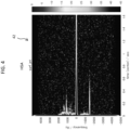
- FIG. 4 shows a spectrogram 42 of HSA.
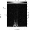
- FIG. 5 shows a spectrogram 44 of HDL, and
- FIG. 6 shows a spectrogram 46 of LDL.
- FID signals respectively for HSA, HDL, and LDL are detected.
- the receiver 14 receives the FID signals respectively for HSA, HDL, and LDL.
- the frequency analyzer 16 executes the short-time Fourier transform on each of the FID signals for HSA, HDL, and LDL, to generate a spectrogram for each of HSA, HDL, and LDL.
- each of the spectrograms 42, 44, and 46 has a plurality of streaks arranged in the direction of the frequency axis. Each streak is parallel to the direction of the horizontal axis, and shows an attenuation characteristic of the FID signal component.
- the multivariable analyzer 18 executes multivariable analysis on a data set formed from the spectrograms 42, 44, and 46, to generate a plurality of combined variables.
- the multivariable analyzer 18 executes the primary component analysis, to identify a first primary component (PC-1) and a second primary component (PC-2), and calculates two loading distributions corresponding to the two primary components and a score of each sample with respect to each primary component.
- the multivariable analyzer 18 represents in a vector format multiple pieces of data (intensities) forming the S spectrograms, and executes the primary component analysis on (SxMxN) pieces of data (that is, data set) represented in the vector format. Through the primary component analysis, the loading distribution is generated for each primary component. The loading distribution is formed from (MxN) loadings represented in the vector format.
- the multivariable analyzer 18 identifies, for each sample, a coordinate corresponding to the score of the sample (more specifically, the first primary component score and the second primary component score) on a two-dimensional coordinate system defined by a first primary component (PC-1) axis and a second primary component (PC-2) axis, and plots a display element on the coordinate, to thereby generate a score plot.
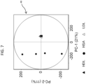
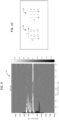
- FIG. 7 shows an example of the score plot.
- the horizontal axis shows the first primary component (PC-1), and the vertical axis shows the second primary component (PC-2).
- a contribution percentage of the first primary component (PC-1) is 21%
- a contribution percentage of the second primary component (PC-2) is 11%.
- the contribution percentage is an indication showing a degree of contribution of the primary component with respect to the data as a whole. The user can empirically recognize importance of the primary component by referring to the contribution percentage.
- Black circle marks show the scores of HSA.
- Black triangle marks show the scores of HDL
- white triangle marks show the scores of LDL.
- the user can recognize a degree of separation of the plurality of samples by referring to the score plot 48.
- the plurality of samples can be evaluated as having similar characteristics.
- the distance between a plurality of plots is long, the plurality of samples can be evaluated as having different characteristics.
- the marks showing HSA are distributed on the score plot 48 while being distanced from the marks showing HDL and the marks showing LDL. Because of this, it can be evaluated on the score plot 48 that HSA, HDL, and LDL are well separated from each other.
- the primary component can be evaluated as significantly contributing to the separation of the plurality of samples.
- the distribution generator 20 generates a loading distribution for a particular primary component based on result of primary component analysis by the multivariable analyzer 18.
- the distribution generator 20 generates the loading distribution for the first primary component (PC-1).
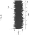
- FIG. 8 shows a loading distribution 50.
- the horizontal axis shows the index
- the vertical axis shows the loading for the first primary component (PC-1).
- the index corresponds to a combination of time and frequency.
- the plot generator 22 generates a loading plot based on the loading distribution 50, and by representing each loading with color or brightness on a two-dimensional coordinate system defined by a time axis and a frequency axis.
- FIG. 9 shows a loading plot 52.
- the plot generator 22 more specifically generates the loading plot 52 through coordinate transformation of the loading distribution 50 having a one-dimensional data format into a loading distribution having a two-dimensional data format.
- the horizontal axis shows the time
- the vertical axis shows the frequency
- a magnitude of the loading for the first primary component (PC-1) is represented with color or brightness.
- the time axis in the loading plot 52 corresponds to the time axis in the spectrogram
- the frequency axis in the loading plot 52 corresponds to the frequency axis in the spectrogram.
- the spectrogram is two-dimensional data.
- the data which is input to the multivariable analyzer 18 and the data which is output from the multivariable analyzer 18 are one-dimensional data. Therefore, the two-dimensional spectrogram must be converted to one-dimensional data before the multivariable analysis is executed.
- the loading distribution which is one-dimensional data must be converted to two-dimensional data.
- FIG. 10 shows a specific example of coordinate transformation.
- Reference numeral 54 shows two-dimensional data
- reference numeral 56 shows one-dimensional data.
- a position in a vertical direction is represented by m
- a position in a horizontal direction is represented by n
- a position in the one-dimensional data 56 is represented by k.
- (n, m) shows a position on the two-dimensional space, or a value at this position.
- (1, 1) shows the position (1, 1) on the two-dimensional space, or a value at the position (1, 1).
- m is a numerical value from 1 to 3
- n is 1 or 2.
- k shows a position on the one-dimensional space, or a value at this position.
- (1) shows a position (1) on the one-dimensional space, or a value at the position (1).
- Equation (1) A relationship between m, n, and k can be represented by following Equation (1).
- k m + n ⁇ 1 ⁇ M
- M is a number of positions in the vertical direction in the two-dimensional data.
- the two-dimensional data is converted into the one-dimensional data
- the one-dimensional data is converted into the two-dimensional data
- the multivariable analyzer 18 converts the spectrogram which is two-dimensional data into one-dimensional data (sub data set) for each sample, according to the above-described relationship.
- the multivariable analyzer 18 executes the primary component analysis on the data set which is a collected group of a plurality of pieces of one-dimensional data corresponding to a plurality of samples.
- the distribution generator 20 generates the loading distribution for each primary component, as a result of the primary component analysis.
- a loading distribution corresponding to the first primary component is used among a plurality of loading distributions corresponding to a plurality of primary components. That is, the plot generator 22 converts the loading distribution corresponding to the first primary component (one-dimensional data) into the loading plot (two-dimensional data) according to the above-described relationship.
- the display controller 26 causes the spectrogram and the loading plot to be displayed side by side on the display unit 28.
- the display controller 26 causes the spectrogram 42 and the loading plot 52 to be displayed side by side on the display unit 28, as shown in FIG. 11 .
- the loading plot 52 is a two-dimensional image having a time axis serving as the horizontal axis and a frequency axis serving as the vertical axis.
- each loading is represented with color or brightness.
- the horizontal axis of the loading plot 52 is the time axis, similar to the horizontal axis of the spectrogram 42
- the vertical axis of the loading plot 52 is the frequency axis, similar to the vertical axis of the spectrogram 42.
- an intensity of a frequency component is represented with color or brightness
- the loading is represented with color or brightness.
- the second coordinate system of the loading plot 52 is the same coordinate system as the first coordinate system of the spectrogram 42, and, thus, the user can easily compare the spectrogram 42 and the loading plot 52.
- the spectrogram 42 and the loading plot 52 are displayed side by side, but this display is merely exemplary.
- the display controller 26 may cause the spectrogram 44 or the spectrogram 46 to be displayed side by side with the loading plot 52 on the display unit 28, in place of the spectrogram 42.
- the display controller 26 causes the designated spectrogram and the loading plot 52 to be displayed side by side on the display unit 28.
- the display controller 26 may cause a plurality of spectrograms and the loading plot 52 to be displayed side by side on the display unit 28.
- the display controller 26 causes the spectrograms 44 and 46 and the loading plot 52 to be displayed side by side on the display unit 28. In this manner, the user can easily compare the plurality of spectrograms and the loading plot.
- the user can perform various investigations based on the two-dimensional loading distribution represented as the loading plot 52.
- the user can perform various investigations based on a change of the loading in the frequency axis direction or the time axis direction (for example, change in color or brightness), based on a position of the frequency axis and/or on the time axis where a characteristic part exists, based on a mutual relationship among a plurality of positions where a plurality of characteristic parts exist, or the like.
- the user can perform various investigations by comparing the two displayed items; that is, the spectrogram and the loading plot.
- the user may specify a position on the frequency axis of a part with a high intensity on the spectrogram, and may observe, on the loading plot, what local state is being caused at the specified position on the frequency axis.
- the user may specify a position (for example, a position on the frequency axis) on the loading plot with a high or low loading, and may observe, on the spectrogram, what local state is being caused at the specified position (for example, position on the frequency axis). This is similarly applicable to the position on the time axis.
- the user may observe a same frequency range on the spectrogram and the loading plot, to compare the change of intensity and the change of loading, or may observe a same time range, to compare the change of intensity and the change of loading. Because the spectrogram and the loading plot have the same coordinate system, these comparisons can be easily made.
- a position on the frequency axis where the intensity becomes high differs depending on the component included in the sample and the structure of the component.
- a component included in the sample can be identified by reference to the intensity distribution in the spectrogram.
- an attenuation rate (change with respect to time) of the NMR signal differs depending on the property of the component
- the position of the intensity distribution on the time axis differs depending on the property of the component included in the sample.
- the user can investigate a difference of the component or a difference of the structure which affects a difference in the attribute among a plurality of samples, by referring to a distribution form (for example, a change of loading in the frequency axis direction, a characteristic part on the frequency axis, or the like) on the loading plot, and comparing the distribution form with a distribution form on the spectrogram (for example, a change of the intensity in the frequency axis direction, a characteristic part on the frequency axis, or the like).
- a distribution form for example, a change of loading in the frequency axis direction, a characteristic part on the frequency axis, or the like
- the user may evaluate a characteristic of each component forming the sample, or analyze or investigate factors (for example, the component and the structure of the sample) that cause a change of the position or a difference of position on the frequency axis on the loading plot, by comparing the attenuation characteristic of each component on the spectrogram and the loading distribution on the loading plot.
- factors for example, the component and the structure of the sample
- the user specifies a position on the frequency axis with a high intensity on the spectrogram.
- the loading plot when the loading is high at a particular position on the frequency axis, the component corresponding to the particular position can be deduced to be significantly contributing to the separation of the plurality of samples. That is, the component is deduced to have a high contribution percentage, for separating the plurality of samples. In this manner, a component which may contribute to separation of the plurality of samples may be deduced by comparing the spectrogram and the loading plot.
- the analysis result of the loading plot may be fed back to the time-frequency analysis by the frequency analyzer 16.
- a characteristic loading distribution is caused at a certain position on the frequency axis on the loading plot (for example, when a high or low loading distribution occurs locally)
- it may be desired to increase the frequency resolution to enable more detailed investigation of the characteristic loading distribution.
- a value which can increase the frequency resolution is set as the frame lengths of the short-time Fourier transform, and the short-time Fourier transform is executed on each FID signal. In this manner, the frequency resolution of the spectrogram corresponding to each sample can be increased.
- the score plot and the loading plot are generated.
- the time-frequency analysis is changed, the time-frequency analysis is re-executed on the plurality of FID signals which are already acquired, in accordance with the changed parameter set, so that a plurality of spectrograms are generated.
- the primary component analysis is re-executed on the data set formed from the plurality of spectrograms, and, as a result of the primary component analysis, a score plot and a loading plot are again generated.
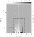
- FIG. 12 shows the loading plot 52.
- the loading plot 52 is displayed on the display unit 28.
- the user designates a time range and a frequency range on the loading plot 52 by manipulating the manipulation unit 30.
- the specifier sets as an analysis region a region 58 defined by the time range and the frequency range designated by the user.
- the frequency analyzer 16 When the analysis region is set, the frequency analyzer 16 re-executes the short-time Fourier transform on a part or a component corresponding to the analysis region in each FID signal, so that a limited spectrogram is generated.
- the multivariable analyzer 18 executes the multivariable analysis on a plurality of limited spectrograms (limited data set) corresponding to the plurality of samples.
- the distribution generator 20 generates a loading distribution based on the result of the multivariable analysis, and the plot generator 22 generates a loading plot based on the loading distribution. In this manner, a loading plot corresponding to the analysis region is generated.
- the loading plot can be called a limited loading plot.
- the parameter set for short-time Fourier transfer is changed prior to the re-execution of the short-time Fourier transform.
- the user designates as the analysis region a region deduced to be contributing to the separation of the plurality of samples, by referring to the loading plot 52. That is, the user designates the analysis region, excluding a region deduced to be not contributing to the separation of the plurality of samples. With this process, the result of the primary component analysis can be improved.
- the analysis region is specified by the region 58 of a quadrangular shape, but alternatively, the analysis region may be specified by a region of a shape other than the quadrangle (for example, a region of a shape of a circle, an ellipse, or any other arbitrary shape).
- the user may designate the analysis region so as to include one or a plurality of characteristic parts.
- the specifier 31 may specify, as the analysis region, a region which satisfies a loading condition.
- the loading condition is satisfied when the loading is within a particular range (for example, a range of greater than or equal to a threshold, a range or less than a threshold, or a range of greater than or equal to a lower limit value and less than an upper limit value).
- the specifier 31 may specify an analysis region to surround a part having a loading of greater than or equal to a threshold.
- a plurality of parts corresponding to the analysis region may be cut out from the plurality of spectrograms which are already generated, without re-executing the time-frequency analysis.
- the multivariable analyzer 18 executes the primary component analysis on a limited data set formed from the plurality of cut-out parts. As a result of the primary component analysis, a new score plot and a new loading plot are generated.
- the cutting-out of the plurality of parts may be executed by the specifier 31 or the multivariable analyzer 18.
- Samples in Example 1 are HSA, HDL, and LDL.
- An objective of Example 1 is executing NMR measurement on albumin and lipoprotein within a human serum, and visualizing a difference between time-frequency characteristics of a plurality of NMR signals acquired from these samples.
- NMR apparatus 10 JNM-ECZ400R manufactured by JEOL Ltd. was used.
- software for data processing and controlling in the NMR apparatus 10 DELTA software (version 5.3.2 (JEOL Ltd.)) was used.
- an application program hereinafter referred to as an "STFT tool" developed for MATLAB TM (The MathWorks, Inc.), and Unscrambler X version 11 (manufactured by Camo Software) were installed.
- a plurality of sample tubes storing the same sample may be prepared, or a plurality of sample tubes storing a plurality of sample solutions having different dilution concentrations may be prepared.
- the STFT tool was started up, the FID signals of the plurality of samples acquired through the measurement were read into the tool, a sampling frequency and a data point number were input to the tool, and then, time-frequency analysis was executed on each of the FID signals.
- the spectrogram 42 illustrated in FIG. 4 is an example of the spectrogram of HSA
- the spectrogram 44 illustrated in FIG. 5 is an example of the spectrogram of HDL
- the spectrogram 46 illustrated in FIG. 6 is an example of the spectrogram of LDL.
- the frequency range and the time range for the analysis target may be narrowed down.
- Unscrambler X was started up, and all of the data (data set) acquired in the time-frequency analysis described above were read into this software. In addition, a data file name, a label for plot display at a later time, and a label for grouping process were input to the software. Then, primary component analysis (PCA) was executed on the data set. By reference to to the score plot which was generated, it was checked whether or not the samples were well separated. More specifically, a score plot was checked having an axis with the largest variance (first primary component axis (PC-1)), and an axis with the second largest variance (second primary component axis (PC-2)).
- PC-1 first primary component axis
- PC-2 second primary component axis
- the score plot 48 illustrated in FIG. 7 is an example of a score plot in Example 1.
- the STFT tool was started up, one spectrogram generated through the time-frequency analysis was opened, and the loading distributions stored in the multivariable analysis 1 described above (the loading distribution of PC-1 and the loading distribution of PC-2) were read. Alternatively, the loading distributions of primary components of PC-3 and subsequent numbers may be read, while viewing the degree of separation and the contribution percentage.
- a loading plot was generated and displayed. The time axis and the frequency axis in the loading plot corresponded to the time axis and the frequency axis in the spectrogram. In the loading plot, it was checked in what region the characteristic appeared.
- the loading plot 52 illustrated in FIG. 9 is an example of the loading plot of Example 1. Based on frequency information of the part where the characteristic appears, it is possible to investigate what component in the sample is related to the characteristic. In addition, based on time information of the part where the characteristic appears, it is possible to investigate from what property the characteristic is derived.
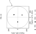
- PLS-DA partial least squares discriminant analysis
- Unscrambler X was started up, and the partial least squares discriminant analysis (PLS-DA) was executed on the data set through a procedure similar to that for the multivariable analysis 1.
- FIG. 13 shows a score plot 60 generated by the partial least squares discriminant analysis (PLS-DA).
- the STFT was started up, one spectrogram generated through the time-frequency analysis was opened through a procedure similar to that described above for the loading plot 1, and the loading distributions stored in the multivariable analysis 2 (the loading distribution of PC-1, and the loading distribution of PC-2) were read.
- a loading plot was generated using the loading distributions which were read, and the loading plot was displayed. In the loading plot, it was checked in what region the characteristic appeared.
- FIG. 14 shows this loading plot 62. Based on frequency information of a part where the characteristic appears, it is possible to investigate what component in the sample is related to the characteristic. Based on time information of the part where the characteristic appears, it is possible to investigate from what property the characteristic is derived.
- Example 1 it was possible to clearly separate the plurality of samples on the score plot. In addition, a difference could be observed among a plurality of frequency positions derived from a plurality of components included in HSA, a plurality of frequency positions derived from a plurality of components included in HDL, and a plurality of frequency positions derived from a plurality of components included in LDL. In other words, it was shown that the loading plot was useful as information for analyzing from what component in each sample the separation on the score plot was derived.
- Example 2 An objective of Example 2 was executing a serum mode analysis on each of a diabetic model mouse (BKS. Cg db/db), and a healthy mouse (JcI:ICR), and judging the onset of arteriosclerosis based on results of the analysis.
- the inventors of the present disclosure postulated a hypothesis that it may be possible to use the analysis method to identify the blood state associated with progress of the arteriosclerosis lesion due to diabetes from healthy states, and analyzed a difference between the serum of a diabetic model mouse (BKS. Cg db/db) and the serum of a healthy mouse (JcI:ICR).
- the diabetic model mouse (BKS. Cg db/db) is a mouse which exhibits a morbid state of the hyperglycemia from an early stage.
- the serum and the carotid tissues were collected from each of the diabetic model mouse (BKS. Cg db/db) and the healthy mouse (JcI:ICR).
- each serum was analyzed using the NMR apparatus, and each carotid tissue was pathologically inspected. It was reviewed whether or not early finding and progress evaluation of the morbid state associated with the arteriosclerosis lesion were possible from the NMR analysis results of the serum, based on two NMR analysis results and two pathological inspection results.
- a diabetic model mouse (BKS. Cg db/db) and a healthy mouse (JcI:ICR) (both purchased from CLEA Japan Inc.) were normally bred in a clean room in an experimental animal management room of Nippon Medical School.
- general pellets (MF, manufactured by Oriental Yeast Co., Ltd.) were used, and the mice were free to eat and drink.
- the blood was centrifugally separated, to separate the serum.
- the separated serum that is, a sample for NMR measurement, was stored at a temperature of -80°C until the time of NMR measurement.
- Example 2 Using a serum sample acquired from the mouse having a symptom of arteriosclerosis, operations and processes similar to those in Example 1 were performed, to generate a spectrogram, a score plot, and a loading plot for each serum sample.
- FIG. 15 shows a spectrogram 64 for BKS.
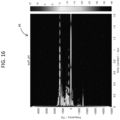
- FIG. 16 shows a spectrogram 66 for Jcl.
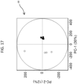
- FIG. 17 shows a score plot 68.
- the score plot 68 is a score plot generated by executing the primary component analysis (PCA).
- FIG. 18 shows a loading plot 70.
- the loading plot 70 is a loading plot generated based on the result of the primary component analysis (PCA).
- FIG. 19 shows another score plot 72.
- the score plot 72 is a score plot generated by the partial least squares discriminant analysis (PLS-DA).
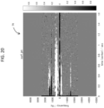
- FIG. 20 shows a loading plot 74.
- the loading plot 74 is a loading plot generated based on a result of the partial least squares discriminant analysis (PLS-DA).
- Example 2 the samples could be clearly separated on the score plot. In addition, a difference in the frequency position derived from each component such as glucose could be read from the loading plot. This matches the medical viewpoint for causes of arteriosclerosis. That is, in Example 2 also, it was shown that the loading plot was useful as information for analyzing from what component in the sample the separation on the score plot was derived.
- An objective of Example 3 is judging a Parkinson's disease (PD) patient using a serum sample.
- DAT-SPECT and MIBG myocardial scintigraphy DAT-SPECT and MIBG myocardial scintigraphy were performed on PD patients and non-PD patients, and it was reviewed whether or not the PD and the non-PD could be identified by the serum sample using the NMR analysis developed by the inventors of the present disclosure.
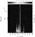
- FIG. 21 shows a spectrogram 76 obtained from the serum of a PD patient.
- FIG. 22 shows a spectrogram 78 obtained from the serum of a non-PD patient.
- FIG. 23 shows a score plot 80.
- the score plot 80 is a score plot generated by the partial least squares discriminant analysis (PLS-DA).
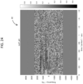
- FIG. 24 shows a loading plot 82.
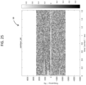
- FIG. 25 shows a loading plot 84.
- the loading plots 82 and 84 are loading plots generated based on the result of the partial least squares discriminant analysis (PLS-DA). In the loading plot 84, a contour line is displayed.
- Example 3 analysis based on PLS-DA was executed using the serum of the PD patient (having abnormal MIBG and abnormal DAT-SPECT), and the serum of the non-PD patient (having normal MIBG and normal DAT-SPECT).
- the groups formed clusters, and different groups were distributed in clearly different regions. Thus, possibility of identifying the PD patient and the non-PD patient through the NMR analysis of the serum was shown.
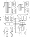
- FIG. 26 shows a flow of a process executed by the processor.
- NMR measurement is executed on a plurality of samples 88, and a plurality of FID signals 90 are thus acquired.
- short-time Fourier transform STFT
- STFT short-time Fourier transform
- a spectrogram 92 is generated based on a sequence of frequency spectra generated by the short-time Fourier transform. That is, a plurality of spectrograms 92 corresponding to the plurality of samples 88 are generated.
- Each spectrogram 92 has a first coordinate system. In the first coordinate system, the horizontal axis is the time axis, and the vertical axis is the frequency axis.
- a data set 94 is formed based on the plurality of spectrograms 92. Specifically, the data set 94 is formed from a plurality of sub data sets 94a corresponding to the plurality of samples. Each sub data set 94a is formed from (mxn) intensities forming each spectrogram.
- the axis i shows an index axis
- the axis j shows a sample axis.
- PCA primary component analysis
- a score plot 98 is generated as a result of the primary component analysis.
- the score plot has a first primary component axis (PC-1) and a second primary component axis (PC-2).
- a general loading plot may be generated.
- the general loading plot is generated based on a loading distribution corresponding to the first primary component, and a loading distribution corresponding to the second primary component, and has the first primary component axis (PC-1) and the second primary component axis (PC-2).
- a loading plot (TF-loading plot) 96 of the embodiment is generated.
- the loading plot 96 corresponding to the first primary component is generated based on a loading distribution 95 corresponding to the first primary component.
- the loading plot 96 has a second coordinate system.
- the horizontal axis is the time axis and the vertical axis is the frequency axis.
- the second coordinate system is identical to the first coordinate system.
- a particular spectrogram 102 is selected from among the plurality of generated spectrograms 92.
- the selected spectrogram 102 and the loading plot 96 are displayed on a display 100.
- a parameter set for the short-time Fourier transform is changed by the user by reference to the loading plot 96.
- the frame length is changed.
- the short-time Fourier transform is re-executed on the plurality of FID signals 90 in accordance with the changed parameter set.
- the primary component analysis is applied to a new data set formed from a plurality of new spectrograms generated through this process.
- an analysis region 106 is set on the loading plot 96.
- the short-time Fourier transform is re-executed on the plurality of FID signals 90.
- a limited data set is formed by a plurality of new spectrograms generated by the re-execution of the short-time Fourier transform.
- the primary component analysis is applied on the limited data set.
- the parameter set may be changed prior to execution of S26.
- a plurality of parts 94 corresponding to the analysis region 106 may be cut out from the plurality of spectrograms 92 which are already generated, without re-executing the short-time Fourier transform.
- the plurality of spectrograms 92 which are already generated are acquired, and in S29, parts 94 corresponding to the analysis region 106 are cut out from the acquired spectrograms 92.
- a limited data set 108 is formed from the plurality of cut-out parts 94.
- the primary component analysis is applied on the limited data set 108.
- a score plot and/or a general loading plot is generated as a result of the primary component analysis.
- a loading plot of the embodiment is generated based on the loading distribution generated by the primary component analysis.
- the loading plot is generated, for example, from the loading distribution corresponding to the first primary component.
- the loading plot is displayed as necessary.
- An analysis region may be set on the loading plot. In this case, the sequence of processes described above are re-executed.
- the content of the spectrogram and the content of the loading plot can be investigated while comparing the spectrogram and the loading plot.
- factors which cause differences in characteristics and attributes among a plurality of samples can be analyzed.
- preemptive medicine that is, a medical care in which a disorder is predicted before a symptom appears, a therapeutic intervention is made, and onset of the disorder is prevented or delayed
- realization of very early diagnosis, determination of therapeutic plans, judgement of therapeutic effect, and prognostic prediction can be expected.
Landscapes
- Physics & Mathematics (AREA)
- Engineering & Computer Science (AREA)
- Health & Medical Sciences (AREA)
- Life Sciences & Earth Sciences (AREA)
- Data Mining & Analysis (AREA)
- High Energy & Nuclear Physics (AREA)
- General Physics & Mathematics (AREA)
- General Health & Medical Sciences (AREA)
- Spectroscopy & Molecular Physics (AREA)
- Theoretical Computer Science (AREA)
- Medical Informatics (AREA)
- Computer Vision & Pattern Recognition (AREA)
- Public Health (AREA)
- Bioinformatics & Computational Biology (AREA)
- Bioinformatics & Cheminformatics (AREA)
- Evolutionary Computation (AREA)
- Evolutionary Biology (AREA)
- Artificial Intelligence (AREA)
- Pathology (AREA)
- Molecular Biology (AREA)
- Chemical & Material Sciences (AREA)
- Epidemiology (AREA)
- Databases & Information Systems (AREA)
- Biomedical Technology (AREA)
- Signal Processing (AREA)
- General Engineering & Computer Science (AREA)
- Analytical Chemistry (AREA)
- Biochemistry (AREA)
- Immunology (AREA)
- Condensed Matter Physics & Semiconductors (AREA)
- Primary Health Care (AREA)
- Bioethics (AREA)
- Biophysics (AREA)
- Software Systems (AREA)
- Biotechnology (AREA)
- Crystallography & Structural Chemistry (AREA)
- Information Retrieval, Db Structures And Fs Structures Therefor (AREA)
- Measurement And Recording Of Electrical Phenomena And Electrical Characteristics Of The Living Body (AREA)
- Investigating Or Analysing Biological Materials (AREA)
Applications Claiming Priority (1)
| Application Number | Priority Date | Filing Date | Title |
|---|---|---|---|
| JP2023097130A JP7755267B2 (ja) | 2023-06-13 | 2023-06-13 | データ処理装置、プログラム及び特性評価方法 |
Publications (1)
| Publication Number | Publication Date |
|---|---|
| EP4478073A1 true EP4478073A1 (en) | 2024-12-18 |
Family
ID=91376774
Family Applications (1)
| Application Number | Title | Priority Date | Filing Date |
|---|---|---|---|
| EP24179890.9A Pending EP4478073A1 (en) | 2023-06-13 | 2024-06-04 | Data processing apparatus, and sample evaluation method |
Country Status (4)
| Country | Link |
|---|---|
| US (1) | US20240420803A1 (cg-RX-API-DMAC7.html) |
| EP (1) | EP4478073A1 (cg-RX-API-DMAC7.html) |
| JP (1) | JP7755267B2 (cg-RX-API-DMAC7.html) |
| CN (1) | CN119128411A (cg-RX-API-DMAC7.html) |
Families Citing this family (1)
| Publication number | Priority date | Publication date | Assignee | Title |
|---|---|---|---|---|
| CN120254610B (zh) * | 2025-05-30 | 2025-09-16 | 山西工程技术学院 | 一种电机异常状态预警系统及方法 |
Citations (4)
| Publication number | Priority date | Publication date | Assignee | Title |
|---|---|---|---|---|
| JP5020491B2 (ja) | 2005-05-02 | 2012-09-05 | 株式会社 Jeol Resonance | Nmrデータの処理装置及び方法 |
| JP5415476B2 (ja) | 2005-05-02 | 2014-02-12 | 株式会社 Jeol Resonance | Nmrデータの処理装置及び方法 |
| WO2015087892A1 (ja) * | 2013-12-10 | 2015-06-18 | 国立大学法人京都大学 | 混合物試料に由来する電磁波信号を処理する方法及び混合物試料の属性を識別する方法 |
| JP2019158868A (ja) | 2018-03-12 | 2019-09-19 | 国立大学法人京都大学 | 特性評価方法、装置およびプログラム |
Family Cites Families (1)
| Publication number | Priority date | Publication date | Assignee | Title |
|---|---|---|---|---|
| CA3224987A1 (en) * | 2021-06-29 | 2023-01-05 | Regeneron Pharmaceuticals, Inc. | Nmr methods for antibody higher order structure comparability |
-
2023
- 2023-06-13 JP JP2023097130A patent/JP7755267B2/ja active Active
-
2024
- 2024-06-04 EP EP24179890.9A patent/EP4478073A1/en active Pending
- 2024-06-12 US US18/740,887 patent/US20240420803A1/en active Pending
- 2024-06-13 CN CN202410760799.8A patent/CN119128411A/zh active Pending
Patent Citations (5)
| Publication number | Priority date | Publication date | Assignee | Title |
|---|---|---|---|---|
| JP5020491B2 (ja) | 2005-05-02 | 2012-09-05 | 株式会社 Jeol Resonance | Nmrデータの処理装置及び方法 |
| JP5415476B2 (ja) | 2005-05-02 | 2014-02-12 | 株式会社 Jeol Resonance | Nmrデータの処理装置及び方法 |
| WO2015087892A1 (ja) * | 2013-12-10 | 2015-06-18 | 国立大学法人京都大学 | 混合物試料に由来する電磁波信号を処理する方法及び混合物試料の属性を識別する方法 |
| JP2015114157A (ja) | 2013-12-10 | 2015-06-22 | 国立大学法人京都大学 | 混合物試料の特性を表現する方法、混合物試料の特性を評価する方法、混合物試料の属性を識別する方法、及び混合物試料に由来する電磁波信号を処理する方法 |
| JP2019158868A (ja) | 2018-03-12 | 2019-09-19 | 国立大学法人京都大学 | 特性評価方法、装置およびプログラム |
Non-Patent Citations (2)
| Title |
|---|
| HIRAKAWA KEIKO ET AL: "Short-time Fourier Transform of Free Induction Decays for the Analysis of Serum Using Proton Nuclear Magnetic Resonance", JOURNAL OF OLEO SCIENCE, vol. 68, no. 4, 1 January 2019 (2019-01-01), JP, pages 369 - 378, XP093219555, ISSN: 1345-8957, DOI: 10.5650/jos.ess18212 * |
| YUI KANAKO ET AL: "Time-frequency analysis reveals an association between the specific nuclear magnetic resonance (NMR) signal properties of serum samples and arteriosclerotic lesion progression in a diabetes mouse model", PLOS ONE, vol. 19, no. 3, 8 March 2024 (2024-03-08), US, pages e0299641, XP093219633, ISSN: 1932-6203, DOI: 10.1371/journal.pone.0299641 * |
Also Published As
| Publication number | Publication date |
|---|---|
| JP2024178751A (ja) | 2024-12-25 |
| JP7755267B2 (ja) | 2025-10-16 |
| US20240420803A1 (en) | 2024-12-19 |
| CN119128411A (zh) | 2024-12-13 |
Similar Documents
| Publication | Publication Date | Title |
|---|---|---|
| Moscoso et al. | Prediction of Alzheimer's disease dementia with MRI beyond the short-term: Implications for the design of predictive models | |
| Charidimou et al. | Total magnetic resonance imaging burden of small vessel disease in cerebral amyloid angiopathy: an imaging-pathologic study of concept validation | |
| EP1171778B1 (en) | Nmr-method for determining the risk of developing type 2 diabetes | |
| Mo et al. | Automated detection of hippocampal sclerosis using clinically empirical and radiomics features | |
| Seewann et al. | Diffusely abnormal white matter in chronic multiple sclerosis: imaging and histopathologic analysis | |
| Henley et al. | Biomarkers for neurodegenerative diseases | |
| Blake et al. | Advanced brain ageing in adult psychopathology: A systematic review and meta-analysis of structural MRI studies | |
| Huang et al. | Identifying resting-state multifrequency biomarkers via tree-guided group sparse learning for schizophrenia classification | |
| WO2015192021A1 (en) | PATTERN ANALYSIS BASED ON fMRI DATA COLLECTED WHILE SUBJECTS PERFORM WORKING MEMORY TASKS ALLOWING HIGH-PRECISION DIAGNOSIS OF ADHD | |
| KR20110086074A (ko) | 지질단백질 인슐린 저항성 지표 및 이와 관련된 방법, 시스템 및 이를 생성하기 위한 컴퓨터 프로그램 | |
| JP7057995B2 (ja) | 哺乳動物におけるうつ病の病態プロファイルを検出するバイオマーカーとその利用 | |
| EP4478073A1 (en) | Data processing apparatus, and sample evaluation method | |
| Borzage et al. | The first examination of diagnostic performance of automated measurement of the callosal angle in 1856 elderly patients and volunteers indicates that 12.4% of exams met the criteria for possible normal pressure hydrocephalus | |
| Al-Iedani et al. | Multi-modal neuroimaging signatures predict cognitive decline in multiple sclerosis: A 5-year longitudinal study | |
| WO2022155566A1 (en) | Magnetic-resonance-based method for measuring microscopic histologic soft tissue textures | |
| Gao et al. | Analysis of white matter tract integrity using diffusion kurtosis imaging reveals the correlation of white matter microstructural abnormalities with cognitive impairment in type 2 diabetes mellitus | |
| Bdaiwi et al. | 129Xe Image Processing Pipeline: An open‐source, graphical user interface application for the analysis of hyperpolarized 129Xe MRI | |
| Reynolds et al. | Quantification of DTI in the pediatric spinal cord: application to clinical evaluation in a healthy patient population | |
| Ekşİ et al. | Differentiation of relapsing-remitting and secondary progressive multiple sclerosis: a magnetic resonance spectroscopy study based on machine learning | |
| Hemond et al. | Paramagnetic rim lesions are highly specific for multiple sclerosis in real-world data | |
| Chu et al. | Hippocampal subregions volume and texture for the diagnosis of mild cognitive impairment | |
| Shen et al. | Correlations between postmortem quantitative MRI parameters and demyelination, axonal loss and gliosis in multiple sclerosis: A systematic review and meta-analysis | |
| US11529054B2 (en) | Method and system for post-traumatic stress disorder (PTSD) and mild traumatic brain injury (mTBI) diagnosis using magnetic resonance spectroscopy | |
| Saatchian et al. | Evaluation of Two Post-Processing Analysis Methods of Proton Magnetic Resonance Spectroscopy in Glioma Tumors | |
| Tinnut et al. | Agreement on grading of normal clivus using magnetic resonance imaging among radiologists |
Legal Events
| Date | Code | Title | Description |
|---|---|---|---|
| PUAI | Public reference made under article 153(3) epc to a published international application that has entered the european phase |
Free format text: ORIGINAL CODE: 0009012 |
|
| STAA | Information on the status of an ep patent application or granted ep patent |
Free format text: STATUS: THE APPLICATION HAS BEEN PUBLISHED |
|
| AK | Designated contracting states |
Kind code of ref document: A1 Designated state(s): AL AT BE BG CH CY CZ DE DK EE ES FI FR GB GR HR HU IE IS IT LI LT LU LV MC ME MK MT NL NO PL PT RO RS SE SI SK SM TR |
|
| STAA | Information on the status of an ep patent application or granted ep patent |
Free format text: STATUS: REQUEST FOR EXAMINATION WAS MADE |
|
| 17P | Request for examination filed |
Effective date: 20250617 |