EP4111147B1 - Verfahren zur erfassung und bildung eines spektrometrischen bildes und spektroskopische messvorrichtung - Google Patents
Verfahren zur erfassung und bildung eines spektrometrischen bildes und spektroskopische messvorrichtung Download PDFInfo
- Publication number
- EP4111147B1 EP4111147B1 EP21708201.5A EP21708201A EP4111147B1 EP 4111147 B1 EP4111147 B1 EP 4111147B1 EP 21708201 A EP21708201 A EP 21708201A EP 4111147 B1 EP4111147 B1 EP 4111147B1
- Authority
- EP
- European Patent Office
- Prior art keywords
- measurement
- spectrometry
- image
- positions
- measurement position
- Prior art date
- Legal status (The legal status is an assumption and is not a legal conclusion. Google has not performed a legal analysis and makes no representation as to the accuracy of the status listed.)
- Active
Links
Images


Classifications
-
- G—PHYSICS
- G01—MEASURING; TESTING
- G01J—MEASUREMENT OF INTENSITY, VELOCITY, SPECTRAL CONTENT, POLARISATION, PHASE OR PULSE CHARACTERISTICS OF INFRARED, VISIBLE OR ULTRAVIOLET LIGHT; COLORIMETRY; RADIATION PYROMETRY
- G01J3/00—Spectrometry; Spectrophotometry; Monochromators; Measuring colours
- G01J3/02—Details
- G01J3/0205—Optical elements not provided otherwise, e.g. optical manifolds, diffusers, windows
- G01J3/0248—Optical elements not provided otherwise, e.g. optical manifolds, diffusers, windows using a sighting port, e.g. camera or human eye
-
- G—PHYSICS
- G01—MEASURING; TESTING
- G01J—MEASUREMENT OF INTENSITY, VELOCITY, SPECTRAL CONTENT, POLARISATION, PHASE OR PULSE CHARACTERISTICS OF INFRARED, VISIBLE OR ULTRAVIOLET LIGHT; COLORIMETRY; RADIATION PYROMETRY
- G01J3/00—Spectrometry; Spectrophotometry; Monochromators; Measuring colours
- G01J3/28—Investigating the spectrum
-
- G—PHYSICS
- G01—MEASURING; TESTING
- G01J—MEASUREMENT OF INTENSITY, VELOCITY, SPECTRAL CONTENT, POLARISATION, PHASE OR PULSE CHARACTERISTICS OF INFRARED, VISIBLE OR ULTRAVIOLET LIGHT; COLORIMETRY; RADIATION PYROMETRY
- G01J3/00—Spectrometry; Spectrophotometry; Monochromators; Measuring colours
- G01J3/28—Investigating the spectrum
- G01J3/2823—Imaging spectrometer
-
- G—PHYSICS
- G01—MEASURING; TESTING
- G01J—MEASUREMENT OF INTENSITY, VELOCITY, SPECTRAL CONTENT, POLARISATION, PHASE OR PULSE CHARACTERISTICS OF INFRARED, VISIBLE OR ULTRAVIOLET LIGHT; COLORIMETRY; RADIATION PYROMETRY
- G01J3/00—Spectrometry; Spectrophotometry; Monochromators; Measuring colours
- G01J3/28—Investigating the spectrum
- G01J3/44—Raman spectrometry; Scattering spectrometry ; Fluorescence spectrometry
-
- G—PHYSICS
- G01—MEASURING; TESTING
- G01J—MEASUREMENT OF INTENSITY, VELOCITY, SPECTRAL CONTENT, POLARISATION, PHASE OR PULSE CHARACTERISTICS OF INFRARED, VISIBLE OR ULTRAVIOLET LIGHT; COLORIMETRY; RADIATION PYROMETRY
- G01J3/00—Spectrometry; Spectrophotometry; Monochromators; Measuring colours
- G01J3/28—Investigating the spectrum
- G01J3/44—Raman spectrometry; Scattering spectrometry ; Fluorescence spectrometry
- G01J3/4406—Fluorescence spectrometry
Definitions
- the present invention relates generally to the field of methods and instruments for acquiring a spectral or hyperspectral image of a sample, based on the use of point-by-point measurement techniques of Raman spectrometry, fluorescence, photoluminescence or cathodoluminescence and image reconstruction.
- It also relates to a spectroscopic measuring device designed to implement such a method.
- a single spectrometric measurement is generally sufficient for the analysis of a spatially homogeneous sample.
- spectrometry imaging techniques are known, based on point-by-point acquisition of spectra and the reconstruction of a spatially resolved spectrometry image. These systems require displacement of the sample relative to the measuring instrument and an excitation beam focused at a point, or scanning of the excitation beam relative to the sample, or a combination of beam scanning and sample displacement.
- the acquisition time of a point-by-point image is determined by the acquisition time of each point and by the number of points in the image.
- the acquisition time of each point is related to the brightness and spectral resolution of each point.
- the number of points in the image depends on the displacement step of the sample relative to the excitation beam or of this beam relative to the sample, which determines the spatial resolution of the image.
- a measuring position represents a particular positioning of the excitation beam relative to the sample for the purpose of performing a spectrometry measurement.
- the contribution of a measurement position is determined based on the initial image.
- the contribution of a measurement position is determined relative to the location of the measurement position on the sample. For example, measurement positions located in an area of the sample with strong intensity variations are considered more contributory than measurement positions located in an area of the sample with constant intensity. In other words, a sample area with uniform intensity can be accurately estimated by one spectrometry measurement, whereas an area with strong spatial intensity variations must be estimated by several spectrometry measurements.
- the method makes it possible to obtain high quality for a given acceleration factor or for a given acquisition time. For example, for a given acceleration factor, the method makes it possible to obtain a spectrometry image of better quality than with a distribution on a predetermined regular grid of the measurement positions to be acquired.
- the analytical instrument also includes a spectrometry device, which allows a spectrometry signal to be acquired at each PM measurement position.
- the spectrometry signal at a point of sample 1 is called a spectrometry measurement.
- the analysis instrument finally includes a computer and processing software to form, using the spectrometry measurements, a hyperspectral spectrometry image or one or more images of sample 1 in different spectral bands or at different wavelengths.
- Each point of the hyperspectral image therefore represents a spectrometry measurement, for example a Raman scattering spectrum, a fluorescence spectrum, a photoluminescence spectrum or a cathodoluminescence spectrum.
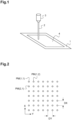
- FIG. 2 illustrates a classic example of a grid of PM measurement positions at which to position the excitation beam 2.
- the PM measurement positions are represented by measurement discs or spots 6 in a plane (XY) of an orthonormal reference frame on the surface of a sample.
- the grid is generally regular, rectangular or square, with a DX pitch along the X axis and a DY pitch along the Y axis.
- the DX pitch is generally chosen equal to the DY pitch.
- a conventional way to form a spectrometry image is to place the incident beam 2 at a measurement position PM(1,1) and acquire a first spectrometry measurement, then move the excitation beam to a measurement position PM(1,2) to acquire a second spectrometry measurement.
- the operations of relative movement of the excitation beam 2 with respect to the sample 1 and acquisition of a spectrometry measurement can then be repeated until a spectrometry measurement is obtained for each measurement position PM of the scanned surface 4 on the sample 1.
- the spatial resolution of the image thus obtained depends on the size of the excitation beam 2 on the sample 1 and the displacement step DX, DY chosen.
- the microscope may be an optical microscope comprising a microscope objective 3 for focusing a laser beam 2 onto a sample 1 to be analyzed.
- the optical microscope is combined with a Raman spectrometer or, respectively, an optical fluorescence or photoluminescence spectrometer, configured to measure a Raman scattering spectrum or, respectively, an optical fluorescence or photoluminescence spectrum in the UV-visible range.
- the microscope may be an X-ray fluorescence microscope, having an X-ray beam focusing and scanning system.
- the X-ray fluorescence microscope is then combined with a spectrometer configured to measure an X-ray spectrum (XRF).
- XRF X-ray spectrum
- the microscope may be a scanning electron microscope (SEM), which incorporates a focusing and scanning system for the electron beam.
- SEM scanning electron microscope
- the scanning electron microscope is then combined with a spectrometer configured to measure an X-ray spectrum (EDX), or a cathodoluminescence spectrum, respectively.
- EDX X-ray spectrum
- cathodoluminescence spectrum a cathodoluminescence spectrum
- Point-by-point spectrometry imaging techniques provide a spatially and spectrally resolved image of a sample.
- the application of Raman microspectrometry allows the analysis of the spatial distribution of chemical composition in an area of a pharmaceutical tablet, with a spatial resolution of the order of ⁇ , where ⁇ represents the wavelength of the excitation beam.
- the spatial resolution of a spectral or hyperspectral image obtained by scanning microscopy is spatially uniform over the entire scanned and analyzed surface.
- the acquisition time of a scanning microspectrometry image increases with the number of points in the spectrometry image thus formed. In practice, the acquisition time is approximately equal to the product of the number of spectrometry measurements times the acquisition time of a spectrometry measurement.
- the analysis instrument of the invention may further advantageously comprise another imaging device making it possible to acquire an initial image, of high spatial resolution, of the area of the sample to be studied.
- This initial structural image may be a video image acquired by means of a CCD camera combined with a scanning microscope.
- a secondary electron detector can quickly provide an initial image of high spatial resolution.
- certain structural details detected on a high-resolution video image such as for example local variations in brightness, may be indicative of variations in measurements obtained by spectrometry, although the video image cannot generally provide spectrometric information.
- FIG. 3 represents a method of acquiring and forming an IS spectrometry image of sample 1.
- the method comprises a step e1 of acquiring an initial image II of an area of the sample 1, the initial image II being composed of pixels, and of defining a maximum set of N, 2 ⁇ N, spectrometry PM measurement positions, each PM measurement position comprising at least one coordinate, representative of the PM measurement position relative to the area of the sample, and at least one intensity, determined on the basis of at least one pixel of the initial image II located in a neighborhood of the PM measurement position.
- initial image acquisition II we mean here the detection of an image of sample 1 on an image sensor, for example of the CCD type or the recovery of an image file of sample 1 obtained on another metrology instrument or from a database comprising an image of the sample 1.
- a digital initial image II is used. If the initial image II detected or collected is analog, it is digitized, so as to obtain a digital initial image II of the sample 1. If necessary, the initial image II is resized according to the area that is to be analyzed by scanning the excitation beam 2 and/or by moving the sample 1 relative to the excitation beam 2.
- the initial image It can be acquired using the spectrometry device of the analysis instrument itself, for example in the case where the initial image II is a single spectral band spectroscopic image. Other modalities require an additional imaging device.
- the initial image II is a video image obtained using a CCD sensor and illuminating the sample with white light.
- the settings of the illumination and the detection system are adjusted so as to increase the contrast of the image and bring out the structural details.
- the intensity, the polarization and/or the wavelength of illumination and/or detection are adjusted so as to obtain a highly contrasted initial structural image.
- FIG. 4 An example of such an initial image is shown in Figure 4 .
- sample 1 symbolizes the letters J, O, B, I and N in dark on a light background.
- the initial image is an RGB image where the intensity of each pixel includes three components, one component for red, one component for green and one component for blue, all coded on 256 bits.
- the initial image II is composed of pixels having one or more intensities, here three intensities.
- the pixels are conventionally distributed in rows and columns.
- the acquisition time of the initial image II is short compared to the acquisition time of the IS spectrometry image.
- the initial image II is for example acquired in a few fractions of a second while the IS spectrometry image is acquired in several minutes.
- step e1 a maximum set of N, 2 ⁇ N, PM spectrometry measuring positions is defined.
- the maximum number of PM measuring positions depends on the DX step along the X axis and the DY step along the Y axis.
- the DX, DY steps are chosen according to the resolution of the analysis instrument.
- the DX, DY steps can for example be determined by the diameter of the measuring spot 6 and by the accuracy of the analysis instrument in the relative displacement of the excitation beam 2 with respect to the sample 1.
- the PM measurement positions therefore define a grid, with steps DX and DY, whose dimensions correspond to the area of sample 1 to be analyzed.
- Each PM measuring position is identified relative to sample 1 by at least one coordinate.
- a measuring position is identified by two coordinates, a CX coordinate along the X axis and a CY coordinate along the Y axis.
- the initial image II is preferably a high-resolution image.
- the resolution of the initial image II is at least as high as the pitch of the grid of the measurement positions PM.
- the coordinates of a measurement position PM can then correspond to a pixel of the initial image II.
- the coordinates of a measurement position PM can then correspond to several pixels.
- the PM measurement positions are displayed superimposed on the initial image II. In order not to overload the figure, only a part of the PM measurement positions are shown. In practice, the grid of PM measurement positions can be at least 4 or 5 times denser than in the example of the Figure 5 .
- two PM measurement positions may be about 4 pixels apart.
- the resolution of the initial image II is then about 16 times higher than the maximum spatial resolution of the spectrometry image IS.
- Each PM measurement position also includes at least one intensity I.
- the intensity of a PM measurement position is calculated on the basis of the intensity of the pixels of the initial image II located in a neighborhood of the measurement point.
- a pixel is for example a neighbor of the measurement position PM closest to it.
- the number of pixels in the neighborhood of a measurement position PM can be estimated by the ratio between the number of pixels of the initial image II and the maximum number N of measurement positions PM.
- the neighborhood can depend on the dimensions of the measurement spot 6.
- the neighborhood of a measurement position PM can thus be defined by the set of pixels included in a circle centered on the measurement position PM and of dimensions substantially similar to the measurement spot 6.
- the intensity of a measurement position PM is calculated by performing an interpolation, for example an average or a bicubic interpolation, of the intensities of the pixels PI located in its neighborhood V.
- the initial image II is subsampled so that the number of pixels after subsampling is equal to the maximum number N of measurement positions PM.
- the intensity of a measurement position PM then corresponds bijectively to the intensity of a pixel of the initial image.
- the intensity of a PM measurement position is therefore of the same nature as the intensity of a pixel in the initial image II.
- the intensity of a PM measurement position can then have the same number of components as the intensity of a pixel.
- the intensity of a PM measurement position comprises three components, a red component IR, a green component IG and a blue component IB.
- the intensity of a PM measurement position has additional components such as a component representative of the average intensity of the pixels in the neighborhood, a component representative of the maximum intensity of the pixels in the neighborhood or a component representative of the minimum intensity of the pixels in the neighborhood.
- additional components can be defined for each color: red, green and blue.
- the method allows each PM measurement position to be assigned a ranking value.
- the method comprises a step e2 of assigning a classification value to each of the N PM measurement positions on the basis of deviations between the PM measurement positions, a deviation between two PM measurement positions being calculated on the basis of a difference in intensity and a difference in coordinates.
- Step e2 allows to order or classify all the PM measurement positions from the most contributing to the least contributing (or vice versa) using the ranking values.
- the ranking value of a PM measurement position allows to quantify the contribution of the PM measurement position in the formation of the IS spectrometry image.
- the contribution of a PM measurement position represents the importance or interest of acquiring a spectrometry measurement at this measurement position to improve the quality of the IS spectrometry image.
- Spectrometry measurements are then acquired based on the ranking values, generally starting with the most contributing measurement positions.
- the spectrometry image is reconstructed and updated in real time based on the actually acquired spectrometry measurements.
- the j+1 th most contributing PM measurement position is the one at which the acquisition of the j+1 th spectrometry measurement will most increase the quality of the IS spectrometry image.
- the quality of the IS spectrometry image at j+1 spectrometry measurements can be estimated based on the initial image II.
- the quality of the IS spectrometry image at j measurements can correspond to a difference with the IS spectrometry image at N spectrometry measurements, i.e. with the IS spectrometry image that would be acquired for an acceleration factor of 1.
- This classification is carried out on the basis of the coordinate(s) and the intensity of the PM measurement position.
- the classification is therefore carried out on the basis of the initial image II.
- the difference between two measurement positions is calculated based on an intensity difference and a coordinate difference.
- the difference is therefore representative of the similarity, both spatial and intensity, between two PM measurement positions. The smaller the difference, the more similar the PM measurement positions are.
- the gap between two PM measurement positions is small, acquiring a spectrometry measurement at only one of the two PM measurement positions is sufficient to construct a spectrometry image.
- the missing spectrometry measurement can be estimated on the basis of the acquired spectrometry measurement.
- One of the two PM measurement positions can then be considered as having little contribution since it is not a priority to acquire a spectrometry measurement there.
- the calculator To calculate a difference between two PM measurement positions, the calculator performs a weighted sum of the square of the intensity difference between the two measurement positions and the square of the coordinate difference between the two measurement positions.
- the intensity components IR1, IG1, IB1, IR2, IG2, IB2 are 8-bit coded values between 0 and 255.
- the coordinates CX1, CY1, CX2, CY2 are the values of the indices defining the location of the measurement position on the grid as represented in Figure 2 .
- the coordinates CX1, CY1, CX2, CY2 are here whole numbers, for example between 1 and the square root of N for a square grid.
- a deviation can be calculated as a weighted sum of the intensity difference between the two measurement positions and the square of the coordinate difference between the two measurement positions.
- a deviation can be calculated as a weighted sum of the average of the intensities of the two measurement positions and the average of the coordinates between the two measurement positions.
- the weighting coefficient R allows the difference in coordinates to be weighted relative to the difference in intensity.
- the weighting coefficient R can be adjusted manually by a user or automatically based on the contrast variations present in the initial image II.
- the weighting coefficient R can take a value between 30 and 100 for an initial image including intensity differences between pixels in light areas and pixels in dark areas greater than 100.
- the weighting coefficient R used for calculating the deviations remains constant during step e2, i.e. for the classification of all the PM measurement positions.
- the weighting coefficient R makes it possible to adapt the calculation of the deviations to sample 1. For example, the more the initial image II presents spatial frequencies The higher the values, the lower the weighting coefficient R. The similarity between two PM measurement positions is then mainly based on intensity. As another example, if the initial image II has small contrast variations over relatively large portions of the initial image II, the weighting coefficient can be high. The similarity between two PM measurement positions is then mainly based on coordinates.
- the value of the weighting coefficient R can also be proportional to an overall contrast of the initial image II to maintain a balance between the difference in coordinates and the difference in intensity. This allows, for example, to assign a significant weighting to the difference in coordinates even in the case of very strong differences in intensity.
- the calculation of the deviation takes into account these additional components.
- the calculator constructs a list S comprising the measurement positions PM whose classification value remains to be assigned, i.e. the measurement positions which remain to be ordered.
- the calculator also constructs a list U comprising the measurement positions PM whose classification value is assigned, i.e. the measurement positions PM already ordered.
- list S contains N PM measurement positions and list U no PM measurement positions.
- list S contains N-j PM measurement positions and list U contains j PM measurement positions.
- each measurement position PM in list S is associated with a total error.
- step e21 determines j total errors. The determination of the total error will be described later. Then, at iteration j of step e22, the calculator selects a PM measurement position, from the j PM measurement positions in list S, based on the total errors, and assigns a ranking value to the selected PM measurement position.
- step e22 the computer selects the PM measurement position associated with the lowest total error.
- the total error here represents the contribution of all already classified PM measurement positions, i.e. those that have received a classification value.
- the contribution of a selected PM measurement position can for example be estimated by the difference between a total error before classification, i.e. before moving this measurement position into the list U, and a total error after classification, i.e. after moving this measurement position into the list U.
- a ranking value is initialized to a predetermined value and at each iteration of step e22, a ranking value strictly lower, respectively higher, than the lowest, respectively highest ranking value is assigned to the PM measurement position associated with the lowest total error.
- Two examples of assigning ranking values are detailed below.
- the calculator then assigns a ranking value to the selected measurement position. For example, the calculator assigns only ranking values that are strictly higher than the previous ones or only ranking values that are strictly lower than the previous ones.
- the previous ranking values are the ranking values already assigned in previous iterations or equal to a predetermined initialization value.
- the PM measurement positions are ordered, at the end of step e2, from the least contributing to the most contributing according to the increasing ranking values.
- a ranking value can be initialized to zero. Then, each selected PM measurement position is assigned a ranking value incremented by +1 relative to the previous one. Thus, the least contributing PM measurement position has a ranking value of 1 and the most contributing a ranking value of N.
- the PM measurement positions are ordered, at the end of step e2, from the most contributing to the least contributing according to the increasing ranking values.
- a ranking value can be initialized to N+1. Then, each selected PM measurement position is assigned a ranking value incremented by -1 relative to the previous one. Thus, the least contributing PM measurement position has a ranking value of N and the most contributing a ranking value of 1.
- this selected PM measurement position is moved from list S to list U.
- list S contains N-j PM measurement positions and list U contains j PM measurement positions.
- the calculator iterates steps e21 and 22 until there are no more PM measurement positions in list S.
- this corresponds to N iterations of steps e21 and e22.
- step e221 the total error associated with the measurement position PM considered is calculated on the basis of the deviations between each measurement position PM of the list U and each measurement position PM of the list U or between each measurement position PM of the list U and measurement positions PM of the list S.
- step e2121 for each measurement position PM in list U, the calculator determines the measurement position in list S with which the deviation is minimum. The calculation of a deviation is detailed later. The value of this minimum deviation is saved.
- step e21 after moving the measurement position PM considered from list S to list U in step e212, list S contains N-j measurement positions PM and list U contains j measurement positions PM.
- the calculator can then calculate (N-j)xj differences between the measurement positions PM of list S and the measurement positions PM of list U.
- the first deviations calculated are those between the measurement position PM from list U and the measurement positions PM from list S located closest in space, i.e. those with which the coordinate difference, hereinafter called distance, is the smallest.
- the deviations are then calculated in ascending order of coordinate difference.
- the minimum deviation is then necessarily part of the deviations already calculated.
- the total error is equal to the sum of each minimum deviation determined in step e2121.
- the calculator calculates the total error associated with a measurement position PM by summing the j minimum deviations for this measurement position PM.
- the calculator moves, in step e213, the PM measurement position considered from list U to list S.
- the calculator therefore associates a total error with each measurement position PM in the list S. As described previously, this then makes it possible to assign a ranking value to the measurement position PM associated with the lowest total error. For example, during iteration j of step e21, this makes it possible to assign a ranking value to the measurement position PM associated with the lowest total error among the j measurement positions in the list S.
- the calculator determines a change in total error associated with each measurement position PM.
- the change in total error is here a difference between two total errors, for two measurement positions PM, for example calculated in accordance with steps e2121 and e2122.
- the change in total error can also be a difference between a first total error, called initial total error, calculated before the measurement position PM considered is moved from list S to list U, and a second total error calculated after the measurement position PM considered is moved from list S to list U.
- the measurement position in list S that is considered the least contributing is the one associated with the lowest total error change. This means that at step e22, the selected measurement position is the one associated with the lowest total error change.
- Calculating total error changes, rather than total errors, allows one to study a variation in total error from one PM measurement position considered to another PM measurement position considered, rather than calculating a total error for each measurement position considered.
- the local error makes it possible to estimate the change in total error since the measurement position considered only has an influence in its vicinity.
- step e21 it is possible to estimate the new initial total error without having to calculate deviations.
- the change in total error associated with the measurement position selected at the previous iteration can be subtracted from the initial error of the previous iteration. This makes it possible to avoid recalculating the initial total error and thus reduce the number of calculations.
- FIG. 6 represents an example of ranking PM measurement positions based on a simulated initial image.
- This simulated initial image shows a dark circle on a light background, i.e., two areas with two distinct intensities.
- the grid on which the N PM measurement positions are placed intentionally has a high pitch to facilitate understanding.
- the six most contributing PM measurement positions are represented in ascending order of ranking value.
- Two measurement positions PM(1), PM(2) can respectively estimate the light area and the dark area represented by hatching.
- the measurement positions PM(3), PM(4), PM(5), PM(6) are the next most contributing because these measurement positions PM(3), PM(4), PM(5), PM(6) can improve the resolution at the edge of the dark area.
- the calculator can define a group of PM measurement positions among the most contributing.
- the calculator selects the P most contributing measurement positions using the ranking values assigned to the PM measurement positions in step e2.
- step e3 the P PM measurement positions of the group are determined according to an ascending, respectively descending, order of the ranking values.
- the calculator increments by +1 the ranking values from the least contributing PM measurement position to the most contributing
- the P measurement positions of the group are those to which the P highest ranking values are assigned.
- the P PM measurement positions of the group are determined according to a decreasing order of ranking values, from the highest to the lowest.
- the P measurement positions of the group are those to which the P lowest ranking values are assigned.
- the P PM measurement positions of the group are determined according to an ascending order of the ranking values, from the lowest to the highest.
- the number P of PM measurement positions can, for example, be determined to achieve a given acceleration factor. For example, to achieve an acceleration factor of 10, the number P of PM measurement positions in the group is equal to N/10. This represents, in step e4, acquisitions of spectrometry measurements at only 10% of the PM measurement positions.
- the number P of PM measuring positions can, for example, be predetermined by a user.
- the number P of PM measuring positions can for example be determined so as to achieve a given acquisition time or a distance traveled by the excitation beam 2 relative to the sample 1 given during step e4. In these cases, the number P of PM measuring positions in the group depends on the location of the PM measuring positions relative to the sample 1.
- the number P of PM measuring positions can also be determined by setting a threshold value on the total errors. After classification in step e2), the total error associated with each PM measuring position can be stored. The number P can then be determined so that the sum of the total errors associated with the measuring positions that are not selected in the group is less than the threshold value.
- An additional criterion can be used when determining the number P of PM measuring positions.
- the number P of PM measuring positions can be determined so that the greatest distance between two PM measuring positions is less than a threshold value.
- the threshold value can, for example, be equal to 15 times the DY or DY step.
- the IS spectrometry image is updated after each new acquisition of a spectrometry measurement.
- the IS spectrometry image is therefore built progressively and dynamically during step e4, i.e. in parallel with the acquisitions of the spectrometry measurements. This makes it possible to continuously improve the quality of the IS spectrometry image during the acquisition of each new spectrometry measurement.
- the order of acquisition of spectrometry measurements can for example be done according to the ranking values assigned to the P PM measurement positions of the group, for example so as to acquire spectrometry measurements from the most contributing PM measurement position to the least contributing.
- a trajectory for carrying out the successive positionings of the excitation beam can be predetermined. This means that the order of acquisition of the spectrometry measurements, at the P PM measurement positions of the group, can be done according to a predetermined trajectory of the excitation beam 2 relative to the sample 1.
- This trajectory can in particular be determined so as to optimize the movement of the excitation beam 2 relative to the sample 1.
- This optimization can for example consist of minimizing the distance traveled by the excitation beam 2 relative to the sample 1 during its successive positioning in all the PM measurement positions of the group.
- This optimization can also, for example, consist of minimizing the number of changes of direction of a sample holder displacement stage.
- This optimization can also consist of minimizing the time required to successively position the excitation beam 2 in all the P PM measurement positions of the group.
- Step e4 includes the construction of the IS spectrometry image.
- the maximum spatial resolution of the IS spectrometry image depends in particular on the maximum set N of measurement positions PM.
- the spatial resolution depends for example on the chosen displacement steps DX, DY.
- the spatial resolution of the IS spectrometry image also depends on the spectrometry measurements that have been acquired.
- the spatial resolution is not homogeneous across the entire IS spectrometry image. Indeed, since the areas of sample 1 with strong spatial intensity variations correspond to the most contributing PM measurement positions, more spectrometry measurements are acquired in these areas, the IS spectrometry image then has a higher spatial resolution in these areas.
- the spatial resolution of the spectrometry image therefore increases locally with each acquisition of a spectrometry measurement at a PM measurement position.
- the IS spectrometry image is composed of spectrometry pixels.
- the IS spectrometry image is here composed of as many spectrometry pixels as there are measurement positions in the maximal set N.
- the IS spectrometry image is composed of spectrometry pixels also arranged in rows and columns.
- Each spectrometry pixel here includes a spectrometry value representative of the spectrometry measurement.
- a spectrometry value can for example represent a spectrum, a portion of a spectrum, the intensity of a narrow spectral band, the intensity of a single wavelength or information from a multivariate analysis or a specific analysis.
- the remaining PM measurement positions are the PM measurement positions for which no spectrometry measurements have been acquired.
- the remaining measurement positions are therefore the PM measurement positions that are not taken into account during step e41.
- the IS spectrometry image is constructed by determining for each PM measurement position, i.e. for each spectrometry pixel, a spectrometry value.
- the computer determines the spectrometry value of each PM measurement position at which a spectrometry measurement was acquired, called acquired measurement position, on the basis of this spectrometry measurement.
- the spectrometry value of an acquired measurement position may for example be equal to the spectrometry measurement or equal to within a factor, i.e. equal to the spectrometry measurement at a wavelength or in a narrow wavelength band.
- the k spectrometry values of the k acquired measurement positions are determined on the basis of their respective spectrometry measurement.
- step e42 the computer determines the spectrometry value of each remaining measurement position, i.e. the PM measurement positions which are not acquired measurement positions. Subsequently, the remaining measurement position "considered” is called the one for which the spectrometry value is determined at a given time.
- the calculator uses at least one spectrometry measurement acquired at an acquired measurement position.
- the acquired measurement position(s) are selected based on their coordinate difference with the remaining measurement position considered.
- the coordinate difference between two PM measurement positions is called the distance.
- the selected spectrometry measurements are the spectrometry measurements acquired at acquired measurement positions having a distance to the remaining measurement position considered less than a minimum distance threshold value. This means that all acquired measurement positions whose distance to the remaining measurement position considered is less than the minimum distance threshold value are selected.
- the spectrometry value can then, for example, be determined on the basis of an average of all selected spectrometry measurements.
- the spectrometry value is here determined on the basis of each selected spectrometry measurement weighted by the deviation between the acquired measurement position at which the selected spectrometry measurement was acquired and the remaining measurement position considered.
- the calculation of the difference between two measurement positions PM is identical to that described previously, i.e. a weighted sum of the square of the difference in intensity between the two measurement positions and the square of the difference in coordinate between the two measurement positions.
- the weighting coefficient R is identical in step e2 and in step e4.
- the weighting coefficient R is different in steps e2 and in step e4.
- the weighting is inversely proportional to the deviation. The further the acquired measurement position is from the remaining measurement position considered, i.e. the greater the deviation, the lower the weight of its spectrometry measurement.
- the spectrometry value is determined based on two spectrometry measurements and a first acquired measurement position has a deviation twice as large as the second with the remaining measurement position considered. Then, when determining the spectrometry value, the spectrometry measurement acquired at the second acquired measurement position can have a weighting twice as large as that of the spectrometry measurement acquired at the first acquired measurement position.
- the spectrometry value of a remaining measurement position is determined on the basis of one or more spectrometry measurements acquired at one or more nearby acquired measurement positions, the proximity between the PM measurement positions being quantified by the deviations between these PM measurement positions.
- spectrometry image is then incomplete. Not assigning a spectrometry value to a remaining measurement position can, for example, be based on a minimum distance threshold value. If no acquired measurement position has a distance to the remaining measurement position that is less than the minimum distance threshold value, no spectrometry value is assigned to the remaining measurement position. This means that if no acquired measurement position is spatially close enough to the remaining measurement position, no spectrometry value is assigned to the remaining measurement position.
- FIGS 7A, 7B, 7C, 7B , 7E and 7F show the IS spectrometry image of sample 1 of the Figure 4 at several acceleration factors.
- the spectrometry values of the remaining measurement positions are equal to the spectrometry measurement of the nearest acquired measurement position.
- the acceleration factor is 100, on the Figure 7B , the acceleration factor is 50, on the Figure 7C , the acceleration factor is 20, on the Figure 7D , the acceleration factor is 10, on the Figure 7E , the acceleration factor is 5 and on the Figure 7F , the acceleration factor is 1.
- the quality of the spectrometry image does not increase regularly.
- the IS spectrometry image constructed on 1% of the most contributing PM measurement positions already allows to distinguish the contrasts of sample 1.
- the quality of the IS spectrometry image increases significantly if it is constructed on 2% or respectively 5% of the PM measurement positions as in Figure 7B and respectively 7C.
- acquire spectrometry measurements in 10%, as in Figure 7D , respectively 20%, as in Figure 7E , or in all measurement positions as in Figure 7F does not significantly increase the quality of the IS spectrometry image since spectrometry measurements have already been acquired at the most contributing PM measurement positions. Even with a high acceleration factor, it is possible to distinguish the word JOBIN here.
- the intensity of a pixel that is not a PS source pixel can be determined based on the nearest PS source pixel, i.e., having the smallest deviation. All pixels whose intensity is estimated based on a PS source pixel form a mesh M associated with this PS source pixel.
- the figure 8 shows in superposition with a part of the initial image II, centered on the letter B, the location of the source pixels PS for an acceleration factor of 20 and their associated mesh M.
- This estimation of the IS spectroscopy image thanks to the estimated structural image IE, can for example help a user to select a given acceleration factor.
- N/100 spectrometry measurements are acquired at the N/100 most contributing PM measurement positions. This allows to obtain an IS spectrometry image with an acceleration factor of 100.
- another N/100 spectrometry measurements are acquired at the next N/100 most contributing measurement positions. The second iteration results in an IS spectrometry image with an acceleration factor of 50.
- the trajectory of excitation beam 2 relative to sample 1 can be optimized during each iteration, i.e. for each group of N/100 PM measurement positions.
- the different groups can also have a different number of PM measurement positions. This is the case, for example, if the number of PM measurement positions per group is determined in such a way as to obtain a given distance traveled by the excitation beam 2 relative to the sample 1.
- a first stopping condition may be that the number of spectrometry measurements to be acquired is predetermined.
- This first stopping condition corresponds, for example, to the case where the desired acceleration factor of the spectrometry image is given. For example, if the acceleration factor to be achieved is 10, the number of spectrometry measurements to be acquired is N/10. Thanks to the acquisition method, the N/10 measurements are then acquired at the N/10 most contributing measurement positions, which makes it possible to obtain a very good quality image for a given acceleration factor.
- the group, determined in step e3 contains a number P of PM measurement positions equal to the number of spectrometry measurements to be acquired and that the trajectory of the excitation beam is optimized over all P PM measurement positions of the group. This makes it possible to obtain an IS spectrometry image at the determined acceleration factor in a minimum of time.
- a second stopping condition may be that the acquisition duration is predetermined.
- the IS spectrometry image acquisition and formation method then makes it possible to obtain an IS spectrometry image of better quality than state-of-the-art methods for a given acquisition duration.
- step e4 here includes sub-step e43.
- step e43 of interpolation of the IS spectrometry image can make it possible to obtain more quickly an interpolated IP image of quality deemed satisfactory by a user.
- the acquisition method comprises a step e11.
- step e11 at least one initial spectrometry measurement is acquired at at least one predetermined initial measurement position, a predetermined ranking value is assigned to each initial measurement position.
- the calculator places the initial measurement positions in the U list since these have ranking values.
- spectrometry measurements are acquired at step e11. These spectrometry measurements are for example distributed on an initial grid with steps greater than the DX and DY steps of the grid on which the set N of PM measurement positions are distributed.
- the initial grid includes N/100 of the N PM measurement positions. Acquiring measurements at these N/100 PM measurement positions allows obtaining an IS spectrometry image with an acceleration factor of 100, i.e. in 1% of the standard acquisition time.
- the group can then be determined on the basis of the measurement positions PM belonging to the region of interest.
- the area of the region of interest is smaller than the area of sample 1. Therefore, only a part of the set of N PM measurement positions lies within the region of interest.
- the PM measurement positions of the group are then selected only from those belonging to the region of interest.
- Determining a region of interest allows to refine the IS spectrometry image, i.e. to increase its spatial resolution, only in a particular location of the sample 1.
- the user can for example define a region of interest where sample 1 has strong contrasts and high spatial frequencies.
- New spectrometry measurements can be acquired outside the region of interest, for example, once all measurement positions in the region of interest have been acquired or after a specified time, or once the part of the IS spectrometry image corresponding to the region of interest reaches a specified acceleration factor.
- a spectrometry measurement is used to estimate the spectrometry values of several neighboring remaining measurement positions. Spatially integrating the measurement allows to obtain an average spectrometry value for this neighborhood. Such an average value can be more representative of sample 1 than a point spectrometry measurement applied to the neighboring spectrometry values.
- the estimated images can be used to estimate whether or not a spectrometry measurement is likely to be used for the determination of spectrometry values of PMR remaining measurement positions.
Landscapes
- Physics & Mathematics (AREA)
- Spectroscopy & Molecular Physics (AREA)
- General Physics & Mathematics (AREA)
- Other Investigation Or Analysis Of Materials By Electrical Means (AREA)
- Analysing Materials By The Use Of Radiation (AREA)
- Investigating, Analyzing Materials By Fluorescence Or Luminescence (AREA)
- Microscoopes, Condenser (AREA)
- Investigating Or Analysing Materials By Optical Means (AREA)
Claims (20)
- Verfahren zur Erfassung und Bildung eines spektroskopischen Bilds (IS) einer Probe (1) mit den folgenden Schritten:e1) Erfassen eines Ausgangsbilds (II) einer Zone der Probe (1), wobei das Ausgangsbild (II) aus Pixeln zusammengesetzt ist, und Definieren einer Gesamtheit von maximal N spektrometrischen Meßpositionen (PM), 2 ≤ N, wobei jede Meßposition (PM) mindestens eine Koordinate (CX; CY), die für die Meßposition (PM) in Bezug auf die Zone der Probe (1) steht, und mindestens eine Stärke (IR1; IR2; IG1; IG2; IB1; IB2), die auf der Grundlage wenigstens eines in einer Umgebung der Meßposition gelegenen Pixels des Ausgangsbilds (II) bestimmt worden ist, aufweist;e2) Zuteilen eines Einstufungswerts an jede der N Meßpositionen (PM) auf der Grundlage von Abständen zwischen den Meßpositionen (PM), wobei ein Abstand zwischen zwei Meßpositionen (PM) auf der Grundlage eines Stärkeunterschieds (IR1; IR2; IG1; IG2; IB1; IB2) und eines Koordinatenunterschieds (CX; CY) berechnet wird;e3) Bestimmen einer Gruppe von P Meßpositionen (PM), 1 ≤ P ≤ N, aus der Gesamtheit von N Meßpositionen (PM) in Abhängigkeit von den im Schritt e2) zugeteilten Einstufungswerten;e4) für jede Meßposition (PM) der im Schritt e3) bestimmten Gruppe nacheinander: Positionieren eines Erregerstrahls (2) auf der Meßposition (PM) in der Zone der Probe (1), Erfassen einer spektrometrischen Messung und Aufbauen des spektrometrischen Bilds (IS) auf der Grundlage der erfaßten spektrometrischen Messung beziehungsweise Messungen.
- Verfahren gemäß Anspruch 1, bei dem der Abstand zwischen zwei Meßpositionen (PM) auf der Grundlage einer gewichteten Summe des Quadrats der Stärkeunterschiede (IR1; IR2; IG1; IG2; IB1; IB2) zwischen den beiden Meßpositionen (PM) und des Quadrats der Koordinatenunterschiede (CX; CY) zwischen den beiden Meßpositionen (PM) berechnet wird.
- Verfahren gemäß einem der Ansprüche 1 bis 2, bei dem sich beim Schritt e2) die zugeteilten Einstufungswerte alle voneinander unterscheiden.
- Verfahren gemäß einem der Ansprüche 1 bis 3, bei dem beim Schritt e3) die P Meßpositionen (PM) der Gruppe in Abhängigkeit von einer aufsteigenden beziehungsweise absteigenden Reihenfolge der Einstufungswerte bestimmt werden.
- Verfahren gemäß einem der Ansprüche 1 bis 4, bei dem beim Schritt e2) eine Liste S, die die Meßpositionen (PM) enthält, deren Einstufungswert noch zuzuteilen ist, und eine Liste U, die die Meßpositionen (PM) enthält, deren Einstufungswert zugeteilt worden ist, eingerichtet werden und die folgenden Schritte mehrfach wiederholt durchgeführt werden:e21) für jede Meßposition (PM) der Liste S: Bestimmen eines Gesamtfehlers durch mehrfach wiederholtes Durchführen der Schritte e211), e212) und e213) des e211) Verlegens der betreffenden Meßposition (PM) der Liste S zur Liste U;e212) Berechnens des zur betreffenden Meßposition (PM) gehörenden Gesamtfehlers auf der Grundlage von Abständen zwischen Meßpunkten (PM) der Liste S und Meßpunkten (PM) der Liste U;e213) Verlegens der betreffenden Meßposition (PM) von der Liste U zur Liste S;e22) Auswählen einer Meßposition (PM) der Liste S auf der Grundlage jedes beim Schritt e21) bestimmten Gesamtfehlers, Zuteilen eines Einstufungswerts an die ausgewählte Meßposition und Verlegen der ausgewählten Meßposition von der Liste S zur Liste U.
- Verfahren gemäß Anspruch 5, bei dem ein Einstufungswert bei einem vorbestimmten Wert angefangen wird, und bei jeder Wiederholung des Schritts e22) ein Einstufungswert, der strikt niedriger beziehungsweise höher als der schwächste beziehungsweise stärkste Einstufungswert ist, der Meßposition (PM) zugeordnet wird, die den kleinsten Gesamtfehler aufweist.
- Verfahren gemäß einem der Ansprüche 5 bis 6, bei dem beim Schritt e212) das Bestimmen des der betreffenden Meßposition zugeordneten gesamten Fehlers die folgenden Schritte aufweist:e2121) für jede Meßposition (PM) der Liste U, Bestimmen der Meßposition (PM) der Liste S, zu der der Abstand der geringste ist, wobei der Wert des Abstands zwischen diesen beiden Meßpositionen (PM) einen minimalen Abstand definiert;e2122) Berechnen des Gesamtfehlers auf der Grundlage jedes beim Schritt e2121) bestimmten minimalen Abstands.
- Verfahren gemäß einem der Ansprüche 1 bis 7, bei dem die Gruppe mindestens drei Meßpositionen aufweist und bei dem ein Weg zum Ausführen der aufeinanderfolgenden Positionierungen des Erregerstrahls (2) vorbestimmt wird.
- Verfahren gemäß einem der Ansprüche 1 bis 8, bei dem die Schritte e3) und e4) mehrfach wiederholt werden und bei dem bei jeder neuen Wiederholung die im Schritt e3) bestimmte Gruppe nur die Meßpositionen (PM) aufweist, für die noch eine spektrometrische Messung zu erfassen ist.
- Verfahren gemäß einem der Ansprüche 1 bis 9, mit einem Schritt e11) des Erfassens wenigstens einer spektrometrischen Messung an mindestens einer vorbestimmten Meßposition, wobei ein vorbestimmter Einstufungswert jeder mindestens einen vorbestimmten Meßposition zugeordnet wird.
- Verfahren gemäß einem der Ansprüche 1 bis 10, bei dem das Aufbauen des spektrometrischen Bilds (IS) die folgenden Schritte aufweist:e41) für jede Meßposition (PM), für die eine spektrometrische Messung erfaßt worden ist, Bestimmen eines Spektrometriewerts auf der Grundlage der besagten spektrometrischen Messung;e42) für jede verbleibende Meßposition, Bestimmen eines Spektrometriewerts auf der Grundlage mindestens einer ausgesuchten spektrometrischen Messung, die in Abhängigkeit vom Unterschied der Koordinaten zwischen der verbleibenden Meßposition und der Meßposition (PM), an der die besagte mindestens eine ausgesuchte spektrometrische Messung erfaßt worden ist, ausgesucht wird.
- Verfahren gemäß Anspruch 11, bei dem beim Schritt e42) die ausgesuchten spektrometrischen Messungen die spektrometrischen Messungen sind, die an Meßpositionen (PM) erhalten worden sind, die einen Unterschied der Koordinaten zur besagten verbleibenden Meßposition von weniger als einem Schwellenwert aufweisen.
- Verfahren gemäß einem der Ansprüche 10 bis 11, bei dem beim Schritt e42) der Spektrometriewert auf der Grundlage jeder ausgesuchten spektrometrischen Messung durch den Abstand zwischen der Meßposition (PM), an der die ausgesuchte Spektroskopische Messung erfaßt worden ist, und der verbleibenden Meßposition bestimmt wird gewichtet wird.
- Verfahren gemäß einem der Ansprüche 1 bis 13, mit einem Schritt e43) der Interpolation des spektrometrischen Bild (IS), bei der eine Anzahl Interpolationskoeffizienten auf der Grundlage der Unterschiede zwischen den Meßpositionen (PM) bestimmt werden.
- Verfahren gemäß einem der Ansprüche 1 bis 14, mit einer Schlußmessung, um beim Schritt e4) das Erfassen zusätzlicher spektrometrischer Messungen zu beenden.
- Verfahren gemäß einem der Ansprüche 1 bis 15, bei dem die Anzahl zu erfassender spektrometrischer Messungen vorbestimmt ist.
- Verfahren gemäß einem der Ansprüche 1 bis 16, bei dem im Ausgangsbild (II) ein Interessengebiet mit nur einem Teil der Meßpositionen (PM) vorbestimmt ist und beim Schritt e3) die Gruppe auf der Grundlage der Meßpositionen (PM) bestimmt wird, die zum Interessengebiet gehören.
- Verfahren gemäß einem der Ansprüche 1 bis 17, bei dem mindestens eine spektrometrische Messung räumlich in einen Sektor der Probe (1) integriert wird.
- Verfahren gemäß einem der Ansprüche 1 bis 18, bei dem das Ausgangsbild (II) unter einer der folgenden Bildgebungsbedingungen erfaßt wird:- spekroskopisches Erfassen in einem oder mehreren vorbestimmten Spektralbändern;- optisches Erfassen als Reflexion oder im Durchlicht;- hyperspektrales Erfassen;- Erfassen mit einem Atomkraftmikroskop ;- Erfassen mit einem Rasterelektronenmikroskop.
- Spektroskopisches Meßgerät mit:- einer zum Erzeugen eines Anregungsstrahls (2) ausgelegten Lichtquelle;- einem zum Aufnehmen einer Probe (1) ausgelegten Träger;- einer Bildaufnahmevorrichtung;- einem Prozessor, der für die Durchführung der Schritte e1) bis e4) des Verfahrens gemäß einem der Ansprüche 1 bis 19 programmiert ist.
Applications Claiming Priority (2)
| Application Number | Priority Date | Filing Date | Title |
|---|---|---|---|
| FR2001912A FR3107591B1 (fr) | 2020-02-26 | 2020-02-26 | Procédé d’acquisition et de formation d’une image de spectrométrie |
| PCT/EP2021/054681 WO2021170717A1 (fr) | 2020-02-26 | 2021-02-25 | Procédé d'acquisition et de formation d'une image de spectrométrie et appareil de mesure spectroscopique |
Publications (2)
| Publication Number | Publication Date |
|---|---|
| EP4111147A1 EP4111147A1 (de) | 2023-01-04 |
| EP4111147B1 true EP4111147B1 (de) | 2025-04-09 |
Family
ID=70154815
Family Applications (1)
| Application Number | Title | Priority Date | Filing Date |
|---|---|---|---|
| EP21708201.5A Active EP4111147B1 (de) | 2020-02-26 | 2021-02-25 | Verfahren zur erfassung und bildung eines spektrometrischen bildes und spektroskopische messvorrichtung |
Country Status (6)
| Country | Link |
|---|---|
| US (1) | US12209908B2 (de) |
| EP (1) | EP4111147B1 (de) |
| JP (1) | JP7751589B2 (de) |
| CN (1) | CN115349078B (de) |
| FR (1) | FR3107591B1 (de) |
| WO (1) | WO2021170717A1 (de) |
Family Cites Families (6)
| Publication number | Priority date | Publication date | Assignee | Title |
|---|---|---|---|---|
| JP5712342B2 (ja) * | 2008-11-27 | 2015-05-07 | ナノフォトン株式会社 | 光学顕微鏡、及びスペクトル測定方法 |
| JP6123360B2 (ja) * | 2013-03-07 | 2017-05-10 | セイコーエプソン株式会社 | 分光測定装置 |
| GB201305171D0 (en) * | 2013-03-21 | 2013-05-01 | Univ Nottingham | Measurement of tissue structures |
| FR3050059B1 (fr) * | 2016-04-07 | 2018-04-20 | Horiba Jobin Yvon Sas | Procede d'acquisition et de formation d'une image de spectrometrie par un echantillonnage spatial adapte |
| JP6422616B1 (ja) * | 2016-12-22 | 2018-11-14 | 国立大学法人 筑波大学 | データ作成方法及びデータ使用方法 |
| EP3351992B1 (de) * | 2017-01-24 | 2019-10-23 | Horiba France SAS | Mikrospektrometriemessverfahren und -system |
-
2020
- 2020-02-26 FR FR2001912A patent/FR3107591B1/fr active Active
-
2021
- 2021-02-25 EP EP21708201.5A patent/EP4111147B1/de active Active
- 2021-02-25 US US17/802,340 patent/US12209908B2/en active Active
- 2021-02-25 CN CN202180024501.1A patent/CN115349078B/zh active Active
- 2021-02-25 JP JP2022550125A patent/JP7751589B2/ja active Active
- 2021-02-25 WO PCT/EP2021/054681 patent/WO2021170717A1/fr not_active Ceased
Also Published As
| Publication number | Publication date |
|---|---|
| JP2023515933A (ja) | 2023-04-17 |
| FR3107591A1 (fr) | 2021-08-27 |
| CN115349078B (zh) | 2026-01-06 |
| US20230003581A1 (en) | 2023-01-05 |
| FR3107591B1 (fr) | 2022-04-08 |
| EP4111147A1 (de) | 2023-01-04 |
| US12209908B2 (en) | 2025-01-28 |
| JP7751589B2 (ja) | 2025-10-08 |
| WO2021170717A1 (fr) | 2021-09-02 |
| CN115349078A (zh) | 2022-11-15 |
Similar Documents
| Publication | Publication Date | Title |
|---|---|---|
| EP2660639B1 (de) | Verfahren und Vorrichtung zur Einzelteilchenlokalisierung mittels Waveletanalyse | |
| Demmerle et al. | Assessing resolution in super-resolution imaging | |
| US9784621B2 (en) | Spectroscopic apparatus and methods | |
| CN1784624A (zh) | 具有波前传感器的扫描激光显微镜 | |
| FR2854953A1 (fr) | Prefiltrage chimique pour differentiation de phase par l'intermediaire d'une spectrometrie par dispersion d'energie simultanee et d'une diffraction par retrodiffusion electronique | |
| EP3100035B1 (de) | Verfahren zum kristallorientierungsmapping einer probe aus einem polykristallinen materials | |
| EP3440443B1 (de) | Verfahren zur erfassung und herstellung eines spektrometriebildes durch angepasste räumliche abtastung | |
| EP4232946B1 (de) | Verfahren zur klassifizierung einer sequenz von eingabebildern, die ein teilchen in einer probe im laufe der zeit darstellen | |
| EP4610626A1 (de) | Verfahren zur spektralen markierung und abbildung von mikropartikeln und system dafür | |
| WO2021170717A1 (fr) | Procédé d'acquisition et de formation d'une image de spectrométrie et appareil de mesure spectroscopique | |
| EP1743192B1 (de) | Verfahren zur korrektur von biparametrischen spektren | |
| CA2778676A1 (fr) | Dispositif et procede de compensation de relief d'images hyper-spectrales | |
| FR3029671B1 (fr) | Procede pour l'analyse assistee par ordinateur d'une ou plusieurs coupes de tissu du corps humain ou animal | |
| JP2022135652A (ja) | 被検物質の分析方法、分析装置、訓練方法、分析システム、及び分析プログラム | |
| EP3427225B1 (de) | Bildverarbeitungsverfahren | |
| EP4166931B1 (de) | Verfahren zur mehrspeziesabbildung eines bereichs aus spektraldaten | |
| EP3764388A1 (de) | Verfahren zur analyse durch elektronenmikroskopie | |
| WO2020025625A1 (fr) | Analyse d'au moins un type de defauts parmi une pluralite de types de defauts entre au moins deux echantillons | |
| WO2025088255A1 (fr) | Spectrométrie par fluorescence de rayons x pour la caractérisation de la microstructure d'un alliage métallique et la détection de ségrégations chimiques | |
| Cointepas | Detection and characterization of exoplanets orbiting M dwarfs with two newnear-infrared instruments: ExTrA and NIRPS. | |
| FR3143757A1 (fr) | Procédé de contrôle de la qualité de fabrication d’une pièce | |
| FR2910673A1 (fr) | Procede de traitement d'image et dispositif implementant ledit procede | |
| EP2232438A1 (de) | VERFAHREN zur Auswertung eines Hydridbilds in einer Metalllegierung, insbesondere in einer Kernbrennstoff-Verkleidungslegierung | |
| FR2710154A1 (fr) | Procédé d'analyse et de quantification des bandes de perlite dans les aciers ferritoperlitiques. |
Legal Events
| Date | Code | Title | Description |
|---|---|---|---|
| STAA | Information on the status of an ep patent application or granted ep patent |
Free format text: STATUS: UNKNOWN |
|
| STAA | Information on the status of an ep patent application or granted ep patent |
Free format text: STATUS: THE INTERNATIONAL PUBLICATION HAS BEEN MADE |
|
| PUAI | Public reference made under article 153(3) epc to a published international application that has entered the european phase |
Free format text: ORIGINAL CODE: 0009012 |
|
| STAA | Information on the status of an ep patent application or granted ep patent |
Free format text: STATUS: REQUEST FOR EXAMINATION WAS MADE |
|
| 17P | Request for examination filed |
Effective date: 20220825 |
|
| AK | Designated contracting states |
Kind code of ref document: A1 Designated state(s): AL AT BE BG CH CY CZ DE DK EE ES FI FR GB GR HR HU IE IS IT LI LT LU LV MC MK MT NL NO PL PT RO RS SE SI SK SM TR |
|
| DAV | Request for validation of the european patent (deleted) | ||
| DAX | Request for extension of the european patent (deleted) | ||
| GRAP | Despatch of communication of intention to grant a patent |
Free format text: ORIGINAL CODE: EPIDOSNIGR1 |
|
| STAA | Information on the status of an ep patent application or granted ep patent |
Free format text: STATUS: GRANT OF PATENT IS INTENDED |
|
| INTG | Intention to grant announced |
Effective date: 20241128 |
|
| GRAS | Grant fee paid |
Free format text: ORIGINAL CODE: EPIDOSNIGR3 |
|
| GRAA | (expected) grant |
Free format text: ORIGINAL CODE: 0009210 |
|
| STAA | Information on the status of an ep patent application or granted ep patent |
Free format text: STATUS: THE PATENT HAS BEEN GRANTED |
|
| AK | Designated contracting states |
Kind code of ref document: B1 Designated state(s): AL AT BE BG CH CY CZ DE DK EE ES FI FR GB GR HR HU IE IS IT LI LT LU LV MC MK MT NL NO PL PT RO RS SE SI SK SM TR |
|
| P01 | Opt-out of the competence of the unified patent court (upc) registered |
Free format text: CASE NUMBER: APP_10941/2025 Effective date: 20250305 |
|
| REG | Reference to a national code |
Ref country code: GB Ref legal event code: FG4D Free format text: NOT ENGLISH |
|
| REG | Reference to a national code |
Ref country code: CH Ref legal event code: EP |
|
| REG | Reference to a national code |
Ref country code: DE Ref legal event code: R096 Ref document number: 602021028868 Country of ref document: DE |
|
| REG | Reference to a national code |
Ref country code: IE Ref legal event code: FG4D Free format text: LANGUAGE OF EP DOCUMENT: FRENCH |
|
| REG | Reference to a national code |
Ref country code: NL Ref legal event code: FP |
|
| REG | Reference to a national code |
Ref country code: AT Ref legal event code: MK05 Ref document number: 1783899 Country of ref document: AT Kind code of ref document: T Effective date: 20250409 |
|
| PG25 | Lapsed in a contracting state [announced via postgrant information from national office to epo] |
Ref country code: FI Free format text: LAPSE BECAUSE OF FAILURE TO SUBMIT A TRANSLATION OF THE DESCRIPTION OR TO PAY THE FEE WITHIN THE PRESCRIBED TIME-LIMIT Effective date: 20250409 Ref country code: PT Free format text: LAPSE BECAUSE OF FAILURE TO SUBMIT A TRANSLATION OF THE DESCRIPTION OR TO PAY THE FEE WITHIN THE PRESCRIBED TIME-LIMIT Effective date: 20250811 Ref country code: ES Free format text: LAPSE BECAUSE OF FAILURE TO SUBMIT A TRANSLATION OF THE DESCRIPTION OR TO PAY THE FEE WITHIN THE PRESCRIBED TIME-LIMIT Effective date: 20250409 |
|
| REG | Reference to a national code |
Ref country code: LT Ref legal event code: MG9D |
|
| PG25 | Lapsed in a contracting state [announced via postgrant information from national office to epo] |
Ref country code: GR Free format text: LAPSE BECAUSE OF FAILURE TO SUBMIT A TRANSLATION OF THE DESCRIPTION OR TO PAY THE FEE WITHIN THE PRESCRIBED TIME-LIMIT Effective date: 20250710 Ref country code: NO Free format text: LAPSE BECAUSE OF FAILURE TO SUBMIT A TRANSLATION OF THE DESCRIPTION OR TO PAY THE FEE WITHIN THE PRESCRIBED TIME-LIMIT Effective date: 20250709 |
|
| PG25 | Lapsed in a contracting state [announced via postgrant information from national office to epo] |
Ref country code: PL Free format text: LAPSE BECAUSE OF FAILURE TO SUBMIT A TRANSLATION OF THE DESCRIPTION OR TO PAY THE FEE WITHIN THE PRESCRIBED TIME-LIMIT Effective date: 20250409 |
|
| PG25 | Lapsed in a contracting state [announced via postgrant information from national office to epo] |
Ref country code: BG Free format text: LAPSE BECAUSE OF FAILURE TO SUBMIT A TRANSLATION OF THE DESCRIPTION OR TO PAY THE FEE WITHIN THE PRESCRIBED TIME-LIMIT Effective date: 20250409 |
|
| PG25 | Lapsed in a contracting state [announced via postgrant information from national office to epo] |
Ref country code: HR Free format text: LAPSE BECAUSE OF FAILURE TO SUBMIT A TRANSLATION OF THE DESCRIPTION OR TO PAY THE FEE WITHIN THE PRESCRIBED TIME-LIMIT Effective date: 20250409 |
|
| PG25 | Lapsed in a contracting state [announced via postgrant information from national office to epo] |
Ref country code: AT Free format text: LAPSE BECAUSE OF FAILURE TO SUBMIT A TRANSLATION OF THE DESCRIPTION OR TO PAY THE FEE WITHIN THE PRESCRIBED TIME-LIMIT Effective date: 20250409 |
|
| PG25 | Lapsed in a contracting state [announced via postgrant information from national office to epo] |
Ref country code: RS Free format text: LAPSE BECAUSE OF FAILURE TO SUBMIT A TRANSLATION OF THE DESCRIPTION OR TO PAY THE FEE WITHIN THE PRESCRIBED TIME-LIMIT Effective date: 20250709 |
|
| PG25 | Lapsed in a contracting state [announced via postgrant information from national office to epo] |
Ref country code: IS Free format text: LAPSE BECAUSE OF FAILURE TO SUBMIT A TRANSLATION OF THE DESCRIPTION OR TO PAY THE FEE WITHIN THE PRESCRIBED TIME-LIMIT Effective date: 20250809 |
|
| PG25 | Lapsed in a contracting state [announced via postgrant information from national office to epo] |
Ref country code: LV Free format text: LAPSE BECAUSE OF FAILURE TO SUBMIT A TRANSLATION OF THE DESCRIPTION OR TO PAY THE FEE WITHIN THE PRESCRIBED TIME-LIMIT Effective date: 20250409 |
|
| PGFP | Annual fee paid to national office [announced via postgrant information from national office to epo] |
Ref country code: GB Payment date: 20251203 Year of fee payment: 6 |
|
| REG | Reference to a national code |
Ref country code: DE Ref legal event code: R097 Ref document number: 602021028868 Country of ref document: DE |
|
| PG25 | Lapsed in a contracting state [announced via postgrant information from national office to epo] |
Ref country code: DK Free format text: LAPSE BECAUSE OF FAILURE TO SUBMIT A TRANSLATION OF THE DESCRIPTION OR TO PAY THE FEE WITHIN THE PRESCRIBED TIME-LIMIT Effective date: 20250409 Ref country code: SM Free format text: LAPSE BECAUSE OF FAILURE TO SUBMIT A TRANSLATION OF THE DESCRIPTION OR TO PAY THE FEE WITHIN THE PRESCRIBED TIME-LIMIT Effective date: 20250409 |
|
| PGFP | Annual fee paid to national office [announced via postgrant information from national office to epo] |
Ref country code: FR Payment date: 20251202 Year of fee payment: 6 |
|
| PG25 | Lapsed in a contracting state [announced via postgrant information from national office to epo] |
Ref country code: CZ Free format text: LAPSE BECAUSE OF FAILURE TO SUBMIT A TRANSLATION OF THE DESCRIPTION OR TO PAY THE FEE WITHIN THE PRESCRIBED TIME-LIMIT Effective date: 20250409 |
|
| PG25 | Lapsed in a contracting state [announced via postgrant information from national office to epo] |
Ref country code: EE Free format text: LAPSE BECAUSE OF FAILURE TO SUBMIT A TRANSLATION OF THE DESCRIPTION OR TO PAY THE FEE WITHIN THE PRESCRIBED TIME-LIMIT Effective date: 20250409 |
|
| PG25 | Lapsed in a contracting state [announced via postgrant information from national office to epo] |
Ref country code: SK Free format text: LAPSE BECAUSE OF FAILURE TO SUBMIT A TRANSLATION OF THE DESCRIPTION OR TO PAY THE FEE WITHIN THE PRESCRIBED TIME-LIMIT Effective date: 20250409 |
|
| PLBE | No opposition filed within time limit |
Free format text: ORIGINAL CODE: 0009261 |
|
| STAA | Information on the status of an ep patent application or granted ep patent |
Free format text: STATUS: NO OPPOSITION FILED WITHIN TIME LIMIT |
|
| REG | Reference to a national code |
Ref country code: CH Ref legal event code: L10 Free format text: ST27 STATUS EVENT CODE: U-0-0-L10-L00 (AS PROVIDED BY THE NATIONAL OFFICE) Effective date: 20260218 |
|
| PGFP | Annual fee paid to national office [announced via postgrant information from national office to epo] |
Ref country code: NL Payment date: 20260218 Year of fee payment: 6 |
|
| 26N | No opposition filed |
Effective date: 20260112 |
|
| PGFP | Annual fee paid to national office [announced via postgrant information from national office to epo] |
Ref country code: DE Payment date: 20251204 Year of fee payment: 6 |
|
| PGFP | Annual fee paid to national office [announced via postgrant information from national office to epo] |
Ref country code: IT Payment date: 20251205 Year of fee payment: 6 |