EP3920113A1 - Optimization apparatus, optimization method, and optimization program - Google Patents
Optimization apparatus, optimization method, and optimization program Download PDFInfo
- Publication number
- EP3920113A1 EP3920113A1 EP21162265.9A EP21162265A EP3920113A1 EP 3920113 A1 EP3920113 A1 EP 3920113A1 EP 21162265 A EP21162265 A EP 21162265A EP 3920113 A1 EP3920113 A1 EP 3920113A1
- Authority
- EP
- European Patent Office
- Prior art keywords
- solution
- constraint
- finish time
- time
- approximate
- Prior art date
- Legal status (The legal status is an assumption and is not a legal conclusion. Google has not performed a legal analysis and makes no representation as to the accuracy of the status listed.)
- Pending
Links
Images






Classifications
-
- G—PHYSICS
- G06—COMPUTING OR CALCULATING; COUNTING
- G06Q—INFORMATION AND COMMUNICATION TECHNOLOGY [ICT] SPECIALLY ADAPTED FOR ADMINISTRATIVE, COMMERCIAL, FINANCIAL, MANAGERIAL OR SUPERVISORY PURPOSES; SYSTEMS OR METHODS SPECIALLY ADAPTED FOR ADMINISTRATIVE, COMMERCIAL, FINANCIAL, MANAGERIAL OR SUPERVISORY PURPOSES, NOT OTHERWISE PROVIDED FOR
- G06Q10/00—Administration; Management
- G06Q10/06—Resources, workflows, human or project management; Enterprise or organisation planning; Enterprise or organisation modelling
- G06Q10/063—Operations research, analysis or management
- G06Q10/0631—Resource planning, allocation, distributing or scheduling for enterprises or organisations
- G06Q10/06315—Needs-based resource requirements planning or analysis
-
- G—PHYSICS
- G06—COMPUTING OR CALCULATING; COUNTING
- G06Q—INFORMATION AND COMMUNICATION TECHNOLOGY [ICT] SPECIALLY ADAPTED FOR ADMINISTRATIVE, COMMERCIAL, FINANCIAL, MANAGERIAL OR SUPERVISORY PURPOSES; SYSTEMS OR METHODS SPECIALLY ADAPTED FOR ADMINISTRATIVE, COMMERCIAL, FINANCIAL, MANAGERIAL OR SUPERVISORY PURPOSES, NOT OTHERWISE PROVIDED FOR
- G06Q10/00—Administration; Management
- G06Q10/06—Resources, workflows, human or project management; Enterprise or organisation planning; Enterprise or organisation modelling
- G06Q10/063—Operations research, analysis or management
- G06Q10/0631—Resource planning, allocation, distributing or scheduling for enterprises or organisations
- G06Q10/06313—Resource planning in a project environment
-
- G—PHYSICS
- G06—COMPUTING OR CALCULATING; COUNTING
- G06F—ELECTRIC DIGITAL DATA PROCESSING
- G06F9/00—Arrangements for program control, e.g. control units
- G06F9/06—Arrangements for program control, e.g. control units using stored programs, i.e. using an internal store of processing equipment to receive or retain programs
- G06F9/46—Multiprogramming arrangements
- G06F9/48—Program initiating; Program switching, e.g. by interrupt
- G06F9/4806—Task transfer initiation or dispatching
- G06F9/4843—Task transfer initiation or dispatching by program, e.g. task dispatcher, supervisor, operating system
- G06F9/4881—Scheduling strategies for dispatcher, e.g. round robin, multi-level priority queues
-
- G—PHYSICS
- G06—COMPUTING OR CALCULATING; COUNTING
- G06E—OPTICAL COMPUTING DEVICES
- G06E1/00—Devices for processing exclusively digital data
- G06E1/02—Devices for processing exclusively digital data operating upon the order or content of the data handled
- G06E1/04—Devices for processing exclusively digital data operating upon the order or content of the data handled for performing computations using exclusively denominational number representation, e.g. using binary, ternary, decimal representation
-
- G—PHYSICS
- G06—COMPUTING OR CALCULATING; COUNTING
- G06F—ELECTRIC DIGITAL DATA PROCESSING
- G06F9/00—Arrangements for program control, e.g. control units
- G06F9/06—Arrangements for program control, e.g. control units using stored programs, i.e. using an internal store of processing equipment to receive or retain programs
- G06F9/46—Multiprogramming arrangements
- G06F9/50—Allocation of resources, e.g. of the central processing unit [CPU]
- G06F9/5005—Allocation of resources, e.g. of the central processing unit [CPU] to service a request
- G06F9/5027—Allocation of resources, e.g. of the central processing unit [CPU] to service a request the resource being a machine, e.g. CPUs, Servers, Terminals
- G06F9/5038—Allocation of resources, e.g. of the central processing unit [CPU] to service a request the resource being a machine, e.g. CPUs, Servers, Terminals considering the execution order of a plurality of tasks, e.g. taking priority or time dependency constraints into consideration
-
- G—PHYSICS
- G06—COMPUTING OR CALCULATING; COUNTING
- G06Q—INFORMATION AND COMMUNICATION TECHNOLOGY [ICT] SPECIALLY ADAPTED FOR ADMINISTRATIVE, COMMERCIAL, FINANCIAL, MANAGERIAL OR SUPERVISORY PURPOSES; SYSTEMS OR METHODS SPECIALLY ADAPTED FOR ADMINISTRATIVE, COMMERCIAL, FINANCIAL, MANAGERIAL OR SUPERVISORY PURPOSES, NOT OTHERWISE PROVIDED FOR
- G06Q10/00—Administration; Management
- G06Q10/04—Forecasting or optimisation specially adapted for administrative or management purposes, e.g. linear programming or "cutting stock problem"
-
- G—PHYSICS
- G06—COMPUTING OR CALCULATING; COUNTING
- G06Q—INFORMATION AND COMMUNICATION TECHNOLOGY [ICT] SPECIALLY ADAPTED FOR ADMINISTRATIVE, COMMERCIAL, FINANCIAL, MANAGERIAL OR SUPERVISORY PURPOSES; SYSTEMS OR METHODS SPECIALLY ADAPTED FOR ADMINISTRATIVE, COMMERCIAL, FINANCIAL, MANAGERIAL OR SUPERVISORY PURPOSES, NOT OTHERWISE PROVIDED FOR
- G06Q10/00—Administration; Management
- G06Q10/06—Resources, workflows, human or project management; Enterprise or organisation planning; Enterprise or organisation modelling
- G06Q10/063—Operations research, analysis or management
- G06Q10/0631—Resource planning, allocation, distributing or scheduling for enterprises or organisations
- G06Q10/06312—Adjustment or analysis of established resource schedule, e.g. resource or task levelling, or dynamic rescheduling
Definitions
- the disclosures herein relate to an optimization apparatus, an optimization method, and an optimization program.
- the resource-constrained project scheduling problem is a problem in combinatorial optimization.
- the resource-constrained project scheduling problem concerns a situation in which constrains are imposed on a plurality of tasks and a plurality of resources, and requires the plurality of resources to be allocated to the plurality of tasks while satisfying the constraints such that the duration of the project is shorter than a target optimization period.
- An example of an objective function used in the resource-constrained project scheduling problem is a project completion time (i.e., the time at which all the tasks are completed).
- the problem that minimizes the makespan is referred to as a makespan minimization problem.
- a metaheuristic algorithm can obtain an optimum solution or a solution sufficiently close to the optimum solution, if given a sufficiently long computational time, through state transitions starting from an initial state to search for solutions attaining successively smaller values of an objective function.
- a solution that is sufficiently close to the optimal solution is not always readily obtained within a practically feasible computational time.
- Examples of an apparatus for performing simulated annealing which is one type of metaheuristic algorithm, include an Ising machine (i.e., Boltzmann machine) using an Ising energy function.
- Ising machine i.e., Boltzmann machine
- the problem to be solved is represented as an Ising model using binary variables.
- various constraints regarding a plurality of tasks and a plurality of resources may be incorporated into an objective function, and, then, the objective function may be minimized to obtain a solution.
- there is a problem in an Ising model in that it is difficult to directly formulate a makespan minimization problem.
- Use of an Ising machine to minimize the value of the objective function C while satisfying the constraints "the completion time of all tasks ⁇ C" and "only one of y i is 1" allows an approximate solution to be obtained in a makespan minimization problem.
- Use of this method entails an increase by n in the number of dimensions of the search space in combinatorial optimization, resulting in a significant decrease in the performance of the Ising model for obtaining a solution.
- a makespan minimization problem may be represented by a different problem as an approximation thereto, thereby allowing a solution to be obtained that is approximate to the solution of the makespan minimization problem.
- the durations of all the individual tasks are added to obtain a sum, and an Ising machine is used to obtain an approximate solution such as to minimize the sum serving as an objective function.
- the sum may vastly differ, even when the makespans are almost the same, between the case in which all the tasks are completed substantially at the same time and the case in which one task is completed significantly later than the other tasks.
- methods of using a different problem as an approximation to a makespan minimization problem cannot produce a highly accurate approximate solution.
- Fig. 1 is a drawing illustrating an example of the hardware configuration of an optimization apparatus for executing an optimization method.
- the optimization apparatus illustrated in Fig. 1 includes a CPU 11, a display unit 12, an input unit 13, a ROM 14, a RAM 15, an HDD 16, a network interface 17, a removable-memory-medium drive 18, and a metaheuristic calculation unit 19.
- the CPU 11 and the metaheuristic calculation unit 19 are arithmetic circuits.
- the input unit 13 provides user interface, and receives various commands for operating the optimization apparatus and user responses responding to data requests or the like.
- the display unit 12 displays the results of processing by the optimization apparatus, and further displays various data that make it possible for a user to communicate with the optimization apparatus.
- the network interface 17 is used to communicates with peripheral devices and with remote locations.
- the optimization apparatus illustrated in Fig. 1 is a computer, and the optimization method is provided as a computer program executable by the optimization apparatus.
- This computer program is stored in a memory medium M that is mountable to the removable-memory-medium drive 18.
- the computer program is loaded to the RAM 15 or to the HDD 16 from the memory medium M through the removable-memory-medium drive 18.
- the computer program may be stored in a memory medium (not shown) provided in a peripheral apparatus or at a remote location, and is loaded to the RAM 15 or to the HDD 16 from the memory medium through the network interface 17.
- the CPU 11 Upon receiving user instruction for program execution from the input unit 13, the CPU 11 loads the program to the RAM 15 from the memory medium M, the peripheral apparatus, the remote memory medium, or the HDD 16. The CPU 11 executes the program loaded to the RAM 15 by use of an available memory space of the RAM 15 as a work area, and continues processing while communicating with the user as such a need arises.
- the ROM 14 stores control programs for the purpose of controlling basic operations of the CPU 48 or the like.
- the metaheuristic calculation unit 19 may be a dedicated hardware specifically designed to execute a metaheuristic algorithm, and may be a dedicated hardware that performs simulated annealing to search for a solution of an Ising problem. In an alternative configuration, the metaheuristic calculation unit 19 may not be provided. In such a case, the CPU 11, which is the processor of a general-purpose computer, functions as a metaheuristic calculation unit to perform a metaheuristic algorithm.
- the metaheuristic algorithm may be simulated annealing, a random walk search algorithm, a genetic algorithm, a stochastic evolution algorithm, taboo search, or the like. It suffices for a metaheuristic algorithm to search in a heuristic manner for a solution (i.e., approximate solution) approximate to the solution that minimizes an objective function.
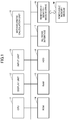
- Fig. 2 is a drawing illustrating an example of the functional configuration of the optimization apparatus.
- the optimization apparatus illustrated in Fig. 2 includes a data storage unit 20, a data acquisition unit 21, a relaxed solution generation unit 22, an optimization data generation unit 23, a metaheuristic calculation unit 24, a solution check unit 25, a solution update unit 26, a termination check unit 27, and a data output unit 28.
- the functional units other than the data storage unit 20 and the metaheuristic calculation unit 24 may be implemented by the CPU 11 illustrated in Fig. 1 .
- the function of the data storage unit 20 may be implemented by the RAM 15 or the HDD 16 illustrated in Fig. 1 .
- the function of the metaheuristic calculation unit 24 may be implemented by the CPU 11 or the metaheuristic calculation unit 19 illustrated in Fig. 1 .
- the data storage unit 20 stores therein a task information database (task information DB) 20A, a resource information database (resource information DB) 20B, relaxed-solution data 20C, and best solution data 20D.
- task information database task information DB
- resource information database resource information database
- the data acquisition unit 21 stores, in the task information database 20A and the resource information database 20B, data regarding individual tasks and data regarding individual resources that are supplied from an external source to define a resource-constrained project scheduling problem. Data regarding constraints on the individual tasks and the individual resources may also be stored in the task information database 20A and the resource information database 20B.
- Fig. 3 is a drawing schematically illustrating an example of a resource-constrained project scheduling problem.
- the resource-constrained project scheduling problem illustrated in Fig. 3 is defined such that tasks #1 through #3 for each of the products A and B and tasks #1 and #2 for a product C are allocated to four facilities 1 through 4.
- a makespan minimization problem in this resource-constrained project scheduling problem is the problem that requires all the tasks to be scheduled such as to make as early as possible a project completion time Tms (i.e., the completion time of the last task completed).
- constraints may be imposed on a plurality of tasks and a plurality of resources.
- a time period indicated as "UNUSABLE" refers to the time period in which the indicated facility cannot be used to perform a task.
- constrains may be imposed on resource usable time.
- constraints may be imposed such that tasks #1, #2, and #3 for a given product may need to be performed in the order named, without overlapping one another in time.
- constraints may be imposed on correspondence between tasks and resources such as the requirement that a particular task can only be performed by a particular resource, and constraints may be imposed on the allowable start time and the required completion time of individual tasks.
- Fig. 4 is a drawing illustrating an example of a binary-variable-based model of the resource-constrained project scheduling problem illustrated in Fig. 3 .
- the resource-constrained project scheduling problem is formulated as a binary-variable-based model, on which an optimization process is performed.
- the binary-variable-based model as illustrated in Fig. 4 is not only applicable to an optimization process performed by an Ising machine, but also applicable to an optimization process performed by a different metaheuristic algorithm.
- binary variables x jmt may be defined.
- Subscript j identifies a task, subscript m identifying a resource, and subscript t identifying a time.
- Each row of the table illustrated in Fig. 4 represents time (by time slots in units of 30 minutes), and each column represents a combination between a task and a facility.
- a column 31 shows a value, at a time t, of a variable x 11t which defines the fact that the task #1 for the product A is allocated to the facility 1.
- the variable for representing the fact that the task #2 for the product B is allocated to the facility 1 is x 51t .
- the length of time required to complete each task (i.e., the required time) is not defined by the value of variable x jmt . Instead, a constant for representing the required time of each task is defined separately. As will be described later, this constant is used to manipulate subscript t, thereby allowing conditions regarding the require time to be specified.
- an objective function that is to be minimized in an optimization process performed by the metaheuristic calculation unit 24 may be defined by binary variable x jmt .
- an objective function E is formulated as a weighting sum of constraint terms Qk multiplied by respective weighting factors c k as follows.
- E c 1 Q 1 + c 2 Q 2 + c 3 Q 3 + c 4 Q 4 + c 5 Q 5 + c 6 Q 6 + c 7 Q 7
- Q 1 ⁇ j ⁇ m ⁇ t ⁇ jst j x j , m
- t Q 2 ⁇ j ⁇ m ⁇ t > jdt j ⁇ jt j x j , m , t
- the constraint term Q1 defines the constraint that each task is started at or after the preset start time (wherein the start time of a task j is the time slot sequence number jst j ).
- the sum is obtained of binary variables x jmt satisfying the condition that the start occurs prior to the time slot sequence number jst j , so that the value of the objective function E increases as a penalty when a value of x jmt subjected to the summation becomes 1.
- the constraint term Q2 defines the constraint that each task is completed by the preset completion time (wherein the completion time of a task j is the time slot sequence number jdt j ).
- the constraint term Q3 defines the constraint that a resource is not used during the time outside the resource usable time (i.e., the time belonging to the complement of the set MT m constituted by time slots allocatable to the resource m).
- the sum of binary variables x jmt is obtained with respect to the time slot sequence numbers belonging to the complement of the set MT m constituted by time slots allocatable to the resource m, so that the value of the objective function E increases as a penalty when a value of x jmt subjected to the summation becomes 1.
- the constraint term Q4 defines the constraint that only the tasks allocatable to a resource (i.e., tasks belonging to the set M_JOB m constituted by tasks executable by a resource m) are allocated to such a resource.
- the sum of binary variables x jmt is obtained with respect to the tasks belonging to the complement of the set M_JOB m constituted by tasks executable by a resource m, so that the value of the objective function E increases as a penalty when a value of x jmt subjected to the summation becomes 1.
- the constraint term Q5 defines the constraint that each task is performed only once.
- the squared term included in the constraint term Q5 is the square of a number obtained by subtracting 1 from the sum that is obtained, with respect to all the resources m and all the time slots t, of binary variables x jmt specifying a particular task j. This squared term becomes 0 when the value of x jmt becomes 1 only once for all the resources m and all the time slots t. In other cases, the squared term assumes a value greater than 0, so that the value of the objective function E increases as a penalty.
- the constraint term Q6 defines the constraint that no resource has two or more tasks simultaneously allocated thereto.
- variable x jmt assumes a value of 1 when the task j starts at the time slot t
- variable x j'mt' assumes a value of 1 when another task j' starts during a period t' between the time slot t and the end of the required time jt j of the task j following the time slot t, which results in the product of these two variables becoming 1.
- allocating two or more tasks simultaneously to a given resource causes the value of the objective function E to increase as a penalty.
- the constraint term Q7 defines a constraint on the order of tasks such that a next task jn starts upon waiting for the time "wait" after a preceding task jp.
- Variable x jpmt assumes a value of 1 when the task jp starts at the time slot t by using the resource m
- a state S having binary variables x jmt as described above may be defined.
- ⁇ is thermodynamic beta (i.e., the reciprocal of absolute temperature).
- min[1, x] assumes a value of 1 or a value of x, whichever is smaller. According to the above formula, a transition to the next state occurs with probability "1" in the case of ⁇ E ⁇ 0, and a transition to the next state occurs with probability exp(- ⁇ E) in the case of 0 ⁇ E.
- the task information database 20A and the resource information database 20B stored in the data storage unit 20 illustrated in Fig. 2 may include data indicative of variables x jmt , the constants, the sets, the objective function, and the like for defining the model as described above.
- the relaxed solution generation unit 22 generates a relaxed solution, i.e., a solution violating a constraint, based on the data indicative of tasks, the data indicative of resources, and the data indicative of constraints stored in the task information database 20A and the resource information database 20B.
- the solution violating a constraint refers to a solution that does not satisfy at least part of the constraints imposed on the tasks and the resources. Such a solution is situated outside the search space satisfying the constraints, and is situated within a search space satisfying at least partially relaxed constraints.
- the term "relaxed solution” and the term "solution violating a constraint" are used to refer to the same meaning.
- the data indicative of a relaxed solution generated by the relaxed solution generation unit 22 is stored as relaxed-solution data 20C in the data storage unit 20.
- the relaxed-solution data 20C includes at least the data indicative of the finish time of a relaxed solution, i.e., the data indicative of the finish time of the task that is completed last among the tasks constituting the relaxed solution.
- a solution satisfying constraints is further defined as a solution satisfying the conditions.
- the solution satisfying constraints may be a solution that satisfies all the constraints defined in an objective function while the solution violating a constraint may be a solution that does not satisfy part of the constraints defined in the objective function.
- data indicative of a solution satisfying constraints obtained by the metaheuristic calculation unit 24 is stored as best solution data 20D in the data storage unit 20.
- the term "solution satisfying constraints” and the term "best solution” are used to refer to the same meaning.
- the best solution data 20D includes at least the data indicative of the finish time of a solution satisfying constraints, i.e., the data indicative of the finish time of the task that is completed last among the tasks constituting the solution satisfying constraints.
- the solution satisfying constraints is defined as a solution that satisfies all the constraints defined in an objective function as described above, the case of the objective function E previously described requires that the solution satisfying constraints is the solution for which the value of the objective function E becomes the smallest value "zero".
- a solution that satisfies part of the constraints e.g., some constraint terms among the constraint terms Q1 through Q7 previously described
- a solution not satisfying such a part of the constraints may be defined as a solution violating a constraint.
- such a part of the constraints that should be satisfied by a solution satisfying constraints may be constraints that need to be satisfied or that are important, and may be defined in accordance with the configuration of the problem. For example, the condition that each task is performed only once and the condition that a resource is not used outside the usable time may be important.
- the relaxed solution generation unit 22 may generate a relaxed solution based on a metaheuristic algorithm.
- a weighing factor c k may be set to zero with respect to one or more constraint terms that are part of the constraint terms Qk included in the objective function E previously described, for example, and that define one or more conditions other than part of the constraints (e.g., the constraint term Q5 requiring each task to be performed only once).
- An approximate solution may then be obtained by minimizing the objective function.
- a solution violating a constraint may be obtained for which the constraint term Q3, for example, requiring a resource to be not used outside the resource usable time assumes a value greater than zero (i.e., the resource is used during the resource unusable time).
- the relaxed solution generation unit 22 may generate a relaxed solution by use of a deterministic algorithm, rather than by use of a metaheuristic algorithm.
- a metaheuristic algorithm in general, is designed such that a probabilistic factor is used to gradually decrease an objective function value while satisfying constraints without being trapped at an unfavorable local solution, thereby generating a satisfactory solution. It suffices for the relaxed solution generation unit 22 to generate a solution without any regard to the constraints. A deterministic algorithm that ignores the constraints may thus readily generate a relaxed solution. Use of a deterministic algorithm allows an initial value of a relaxed solution to be easily obtained in an efficient manner.
- the optimization data generation unit 23 Based on the data stored in the data storage unit 20, the optimization data generation unit 23 generates input data used in an optimization process performed by the metaheuristic calculation unit 24.
- the input data generated by the optimization data generation unit 23 includes the end time of a target optimization period which is used in the optimization process performed by the metaheuristic calculation unit 24.
- the end time of a target optimization period is equal to the sequence number of the last time slot belonging to the set T of time slots subjected to the optimization process, which is one of the constants described in connection with the model formulation of a resource-constrained project scheduling problem previously described. This time is obtained based on the relaxed-solution data 20C and the best solution data 20D as will be described later.
- the end time of a target optimization period is set between the finish time of a relaxed solution indicated by the relaxed-solution data 20C and the finish time of a best solution indicated by the best solution data 20D.
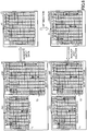
- Fig. 5 is a drawing illustrating an example of input data that is used in an optimization process and that is generated based on a relaxed solution and a best solution.
- Fig. 5 for the sake of convenience of explanation, only the data indicative of the tasks #1 through #3 for the product A (i.e., the tasks A1 through A3) are illustrated, and the relaxed-solution data 20C and the best solution data 20D are stored in the data storage unit 20.
- the relaxed-solution data 20C specifies the state of a relaxed solution based on the model using binary variables x jmt previously described.
- the best solution data 20D specifies the state of a best solution based on the model using binary variables x jmt .
- the arrays of values of variables x jmt are illustrated by using a table format similar to that of Fig. 4 for the purpose of allowing the state of solutions to be visually recognized.
- the time periods highlighted in dot shading indicate the periods during which the indicated resources cannot be used.
- a distinction between the solution satisfying constraints and the solution violating a constraint is made according to whether the constraint term Q3 previously described is satisfied, i.e., whether the indicated resources are used only during the resource usable time.
- the time at which the task A3 i.e., the task #3 for the product A
- this relaxed solution is a solution violating a constraint for which the constraint term Q3 previously described has a value greater than zero (i.e., the resource is used during the resource unusable time).
- this best solution is a solution satisfying constraints for which the constraint term Q3 previously described has a value of zero (i.e., the resource is used only during the resource usable time).
- the finish time of the task that is completed last among the tasks included in the relaxed solution is the finish time T1 of the relaxed solution. Further, the finish time of the task that is completed last among the tasks included in the best solution is the finish time T2 of the best solution.
- the time slot sequence number of the finish time T1 is 9, and the time slot sequence number of the finish time T2 is 15.
- the optimization data generation unit 23 generates input data 41 for an optimization process based on the relaxed-solution data 20C and the best solution data 20D stored in the data storage unit 20.
- the input data 41 represents tasks, facilities, and time slots subjected to an optimization process based on the model using binary variables x jmt .
- the input data 41 defines the configuration of a problem in which scheduling is made to allocate tasks to facilities at particular time slots.
- the arrays of values of variables x jmt are illustrated by using a table format similar to that of Fig. 4 for the purpose of allowing the state of variables to be visually recognized.
- the input data 41 defines that an optimization process is to be performed such that three tasks are allocated to three facilities between the time slot sequence number 0 at 8:30 and the time slot sequence number 13 at 15:00. It may be noted that the set T of time slots subjected to an optimization process, as previously described, accordingly includes, as elements of the set, the time slots from 8:30 to 15:00.
- the optimization data generation unit 23 generates the input data 41 such that the time of the last time slot of the input data 41 (i.e., the end time of a target optimization period) is situated between the finish time T1 of the relaxed solution and the finish time T2 of the best solution described above.
- the interval between the finish time T1 and the finish time T2 may be divided with a predetermined ratio (e.g., 1:1), so that the end time of a target optimization period is set at the point of the divide. Setting the end time of a target optimization period according to a predetermined ratio allows a simple process to generate the input data 41 in an efficient manner.
- the metaheuristic calculation unit 24 Based on the input data 41 generated as described above, performs an optimization process as will be described below.
- the metaheuristic calculation unit 24 performs a heuristic optimization process based on the data configured by the optimization data generation unit 23, thereby generating an approximate solution that minimizes the value of a designed objective function.
- tasks are scheduled such that the finish time of any given task is no later than the end time of a target optimization period set by the optimization data generation unit 23.
- the optimization process evaluates only those schedules in which all the tasks are completed before or at the time slot of 15:00. This is achieved by setting the last time slot of the set T of time slots subjected to an optimization process to the end time of a target optimization period.
- An approximate solution generated by the metaheuristic calculation unit 24 may sometimes be a solution violating a constraint and may sometimes be a solution satisfying constraints, depending on various conditions including the end time of a target optimization period.
- a solution violating a constraint or a solution satisfying constraints generated by the metaheuristic calculation unit 24 are used by the solution update unit 26 to update the relaxed-solution data 20C or the best solution data 20D, as will be described later in detail.
- the solution update unit 26 replaces the relaxed-solution data 20C with the data indicative of a solution violating a constraint upon the occurrence of a solution violating a constraint, and replaces the best solution data 20D with the data indicative of a solution satisfying constraints upon the occurrence of a solution satisfying constraints.
- the calculation of an approximate solution by the optimization process of the metaheuristic calculation unit 24 and the updating of the relaxed-solution data 20C and the best solution data 20D by the solution update unit 26 are repeatedly performed, thereby successively updating solutions.
- the optimization data generation unit 23 and the metaheuristic calculation unit 24 function as an optimization process unit 30.
- the optimization process unit 30 performs an optimization process in a resource-constrained project scheduling problem to generate an approximate solution based on the task information database 20A, the resource information database 20B, relaxed-solution data 20C, and the best solution data 20D. Specifically, the optimization process unit 30 sets the end time of a target optimization period at a point between the first finish time that is the finish time of a preceding solution violating a constraint and the second finish time that is the finish time of a preceding solution satisfying constraints, followed by obtaining an approximate solution by use of a metaheuristic algorithm.
- the optimization process unit 30 sets the end time of a target optimization period at a point between the finish time (i.e., the first finish time) of a solution indicated by the latest relaxed-solution data 20C and the finish time (i.e., the second finish time) of a solution indicated by the latest best solution data 20D, followed by obtaining an approximate solution by use of a metaheuristic algorithm.
- the term "approximate solution” refers to a solution that does not guarantee the occurrence of the minimum value of an objective function for optimization, and that can be regarded as a proper approximation to the optimum solution minimizing the objective function.
- the optimization process makes successive state transitions in the search space such as to stochastically decrease the value of the objective function.
- the state observed at that instance may be output as an approximate solution.
- the optimization process unit 30 may perform the optimization process for a predetermined duration determined in advance, and, then, may output the state observed at that instance as an approximate solution.
- the optimization process unit 30 may detect the event in which the value of an optimization process becomes lower than or equal to a predetermined value determined in advance, and, then, may output the state observed at that instance as an approximate solution.
- respective initial value data are used as the finish time of the relaxed-solution data 20C and the finish time of the best solution data 20D.
- An initial value serving as the first relaxed-solution data 20C is the relaxed-solution data 20C generated by the relaxed solution generation unit 22 as previously described.
- the optimization process unit 30 may generate a solution satisfying constraints.
- the end time of a target optimization period may be set to a sufficiently large value (i.e., a sufficiently late point in time) that is feasible and sensible from the viewpoint of making a time schedule for tasks.
- weighting factors for relevant constraints included in an objective function for optimization may be set to sufficiently large values, thereby ensuring that a solution satisfying constraints is sure to be obtained.
- the solution search space used in the optimization process may be limited to the space that satisfies constraints, so that state transitions made in the optimization process may be allowed only when the next state satisfy the constraints.
- Data indicative of the solution satisfying constraints generated first by the optimization process unit 30 is stored as the initial value data of the best solution data 20D in the data storage unit 20.
- the solution check unit 25 determines whether the approximate solution generated by the optimization process unit 30 is a solution violating a constraint or a solution satisfying constraints. In doing so, the solution check unit 25 may determine that a solution satisfying all the constraints (e.g., all the constraint terms Q1 through Q7 previously described) is a solution satisfying constraints, and may determine that a solution not satisfying at least some of the constraints is a solution violating a constraint. Alternatively, the solution check unit 25 may determine that an approximate solution satisfying predetermined constraints among a plurality of constraints is a solution satisfying constraints, and may determine that an approximate solution not satisfying these predetermined constraints is a solution violating a constraint.
- the solution check unit 25 may determine that an approximate solution satisfying predetermined constraints among a plurality of constraints is a solution satisfying constraints, and may determine that an approximate solution not satisfying these predetermined constraints is a solution violating a constraint.
- the solution check unit 25 may determine that a solution satisfying predetermined constraint terms among the constraint terms Q1 through Q7 previously described is a solution satisfying constraints, and may determine that a solution not satisfying at least some of these predetermined constraint terms is a solution violating a constraint.
- an obtained approximate solution is likely to be a solution violating a constraint.
- an obtained approximate solution is likely to be a solution satisfying constraints.
- the solution update unit 26 updates the first finish time by using the finish time of the approximate solution when the approximate solution is a solution violating a constraint, and updates the second finish time by using the finish time of the approximate solution when the approximate solution is a solution satisfying constraints. Namely, in the case in which the approximate solution generated by the optimization process unit 30 is a solution violating a constraint, data of the approximate solution is used to update (i.e., replaces) the relaxed-solution data 20C (including the data indicative of the finish time of a solution) stored in the data storage unit 20.
- data of the approximate solution is used to update (i.e., replaces) the best solution data 20D (including the data indicative of the finish time of a solution) stored in the data storage unit 20.
- Fig. 6 is a drawing illustrating the updating of either one of relaxed-solution data and best solution data by use of data indicative of a generated approximate solution.
- the same or corresponding elements as those of Fig. 5 are referred to by the same or corresponding numerals, and a description thereof will be omitted as appropriate.
- the metaheuristic calculation unit 24 Based on the input data 41 generated by the optimization data generation unit 23 as described in connection with Fig. 5 , the metaheuristic calculation unit 24 performs an optimization process to generate an approximate solution.
- an approximate solution 51 obtained by the metaheuristic calculation unit 24 indicates that all the tasks are performed during the resource usable time.
- the solution check unit 25 may determine that the obtained approximate solution 51 is a solution satisfying constraints (i.e., best solution).
- the solution update unit 26 replaces the best solution data 20D stored in the data storage unit 20 with the data indicative of the obtained approximate solution 51.
- the best solution data 20D in the data storage unit 20 is updated, so that the finish time T2 of the best solution is changed from the time slot sequence number 15 to the time slot sequence number 11.
- the optimization apparatus illustrated in Fig. 2 successively updates the finish time (i.e., the first finish time) of a solution indicated by the relaxed-solution data 20C and the finish time (i.e., the second finish time) of a solution indicated by the best solution data 20D, and causes the metaheuristic calculation unit 24 to produce an approximate solution repeatedly while performing such updating.
- the finish time (i.e., the first finish time) of a solution indicated by the relaxed-solution data 20C and the finish time (i.e., the second finish time) of a solution indicated by the best solution data 20D gradually approach each other.
- the termination check unit 27 checks whether a difference between the finish time (i.e., the first finish time) of a solution indicated by the relaxed-solution data 20C and the finish time (i.e., the second finish time) of a solution indicated by the best solution data 20D becomes less than or equal to a predetermined value.
- the difference in time becomes less than or equal to the predetermined value, i.e., when the first finish time and the second finish time become sufficiently close to each other or equal to each other
- the termination check unit 27 terminates the process of obtaining a solution approximate to the makespan minimum solution performed by the optimization apparatus.
- the solution indicated by the best solution data 20D at the time the two finish times become equal or substantially equal to each other is consequently a proper approximate solution for the makespan minimum solution.
- the termination check unit 27 may check whether a difference between the second finish time and the end time of a target optimization period becomes less than or equal to a predetermined value, and may terminate the process of obtaining a solution approximate to the makespan minimum solution based on such a check result.
- the first finish time is denoted as T1
- the second finish time is denoted as T2
- the makespan minimum solution i.e., ideal solution
- T IDEAL makespan minimum solution
- T1 is equal to the finish time of a solution when it is not possible (or is difficult) to obtain a solution satisfying constraints
- T2 is equal to the finish time of a solution when a solution satisfying constraints is successfully obtained.
- the condition of T1 ⁇ T2 is thus satisfied with high probability.
- T END the condition of T END ⁇ T2 is satisfied because T END is set between T1 and T2.
- the finish time of an approximate solution to update T2 is always earlier than T END , so that T2 is always updated to an earlier time whenever it is updated. Accordingly, T2 monotonously decreases (i.e., gradually moves to earlier time with certainty).
- the makespan minimum solution is the solution that has the earliest finish time among all the possible solutions satisfying constraints, so that the condition of T IDEAL ⁇ T2 is satisfied. Since T2 is selected from the finish times of all the solutions satisfying constraints such as to monotonously decrease, T2 approaches T IDEAL promptly with certainty. When T2 becomes substantially equal to T1, the value of T2 is consequently a highly accurate approximate value for T IDEAL .
- T2 approaches T IDEAL promptly with substantial certainty similarly to the manner previously described.
- T2 becomes substantially equal to T1
- the value of T2 is consequently a highly accurate approximate value for T IDEAL .
- the data output unit 28 outputs data indicative of a solution that is obtained in the manner described above and that is approximate to the makespan minimum solution.
- the output data may be supplied to a display screen via the display unit 12 illustrated in Fig. 1 , to the HDD 16, to the memory medium M via the removable-memory-medium drive 18, or to an external device via the network interface 17.
- the optimization apparatus illustrated in Fig. 2 successively updates the finish time of a solution indicated by the relaxed-solution data 20C and the finish time of a solution indicated by the best solution data 20D, and causes a metaheuristic optimization process to produce an approximate solution repeatedly while performing such updating.
- the objective function subjected to minimization in the metaheuristic optimization process does not include a term whose value decreases as the makespan (i.e., the project completion time) becomes earlier and earlier.
- the optimization apparatus illustrated in Fig. 2 does not evaluate a makespan, and obtains an approximate solution for a given end time of a target optimization period which minimizes the objective function that defines constraints. Then, based on the approximate solution obtained by the current-round optimization process, the end time of a target optimization period is shifted in the direction where a solution approximate to the makespan minimum solution is situated or is likely situated, and, then, a next-round optimization process is performed with respect to the shifted end time of a target optimization period.
- the shifting and updating of an end time of a target optimization period as described above allows an approximate solution obtained by an optimization process to move closer to a solution approximate to the makespan minimum solution.
- the optimization apparatus illustrated in Fig. 2 does not need to incorporate a makespan evaluation index for a resource-constrained project scheduling problem indirectly, or as an approximation, into the objective function, thereby avoiding the lowering of efficiency of a metaheuristic optimization process and the lowering of accuracy of a solution.
- the end time of a target optimization period is shifted by the procedure similar to binary search.
- the total number of time slots is N, therefore, performing an optimization process a number of times approximately equal to Log 2 N enables the obtainment of a proper approximate solution for makespan minimization.
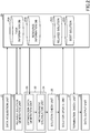
- Fig. 7 is a flowchart illustrating an example of the procedure of an approximation method.
- the approximation method illustrated in Fig. 7 may be performed by the function units illustrated in Fig. 2 by use of the hardware illustrated in Fig. 1 .
- step S1 the data acquisition unit 21 receives input data inclusive of resource information, task information, time information, and the like.
- the data received by the data acquisition unit 21 is stored in the data storage unit 20.
- step S2 the relaxed solution generation unit 22 derives a solution by allocating resources to tasks by disregarding constraint violation, followed by storing data indicative of the derived solution as the relaxed-solution data 20C in the data storage unit 20.
- the relaxed solution generation unit 22 may use a deterministic algorithm to allocate resources to tasks.
- step S3 the metaheuristic calculation unit 24 derives a solution satisfying constraints by use of an Ising machine, for example, followed by storing data indicative of the derived solution as the best solution data 20D in the data storage unit 20.
- step S4 the optimization data generation unit 23 sets the finish time T1 to the task completion time of a solution indicated by the relaxed-solution data 20C, and sets C1 to the amount of constraint violation of the solution indicated by the relaxed-solution data 20C.
- the amount of constraint violation is a value indicative of the degree to which a solution violating a constraint violates constraints.
- the end time of a target optimization period is not set at the point in time at which the interval between the first finish time and the second finish time is divided with a predetermined ratio, but is set based on the amount of constraint violation and the amount of constraint conformity margin, which will be described later.
- the amount of constraint violation may be the total number of time slots at which constraint is violated by the combination of a task and a resource (i.e., facility) in a relaxed solution, for example.
- the constraint requiring that a task is allocated to a resource only during the resource usable time may be taken into consideration, for example.
- the number of time slots at which such a constraint is violated by allocation is used as the amount of constraint violation.
- the task A3 is allocated to the facility 3 at the time slot sequence numbers "3" and "4" (i.e., 10:00 and 10:30)) which are resource unusable time.
- the amount of constraint violation may be 2.
- step S5 the optimization data generation unit 23 sets the finish time T2 to the task completion time of a solution indicated by the best solution data 20D, and sets C2 to the amount of constraint conformity margin of the solution indicated by the best solution data 20D.
- the amount of constraint conformity margin is a value indicative of the degree to how much margin exists for a solution satisfying constraints to satisfy constraints.
- the optimization data generation unit 23 calculates the end time of a target optimization period based on the amount C1 of constraint violation and the amount C2 of constraint conformity margin, and rounds up the fraction as appropriate, followed by setting T END to the obtained end time of a target optimization period.
- the end time of a target optimization period may be set at a point in time that divides the interval between the first finish time T1 and the second finish time T2 according to the ratio corresponding to the amount C1 of constraint violation of a relaxed solution (i.e., an initial value or a preceding solution violating a constraint) and the amount C2 of constraint conformity margin of a best solution (i.e., an initial value of a preceding solution satisfying constraints).
- the end time T END of a target optimization period may be calculated by use of the following formula, for example.
- T END T 1 + T 2 ⁇ T 1 C 1 / C 1 + C 2
- Calculating the end time of a target optimization period in this manner allows the end time of a target optimization period to be set to a relatively late time (i.e., the time closer to T2 than to T1) when the amount C1 of constraint violation is relatively large, i.e., when the finish time T1 of a relaxed solution is situated at too early a time. Further, the end time of a target optimization period is set to a relatively early time (i.e., the time closer to T1 than to T2) when the amount C2 of constraint conformity margin is relatively large, i.e., when the finish time T2 of a best solution is so late as to provide a sufficient margin.
- a relatively late time i.e., the time closer to T2 than to T1
- the end time of a target optimization period is set to a relatively early time (i.e., the time closer to T1 than to T2) when the amount C2 of constraint conformity margin is relatively large, i.e., when the finish time T2 of a
- the end time T END of a target optimization period may be calculated by use of the following formula, for example.
- T END T 1 + T 2 ⁇ T 1 1 / 3 when C 1 ⁇ C 2
- T END T 1 + T 2 ⁇ T 1 2 / 3 when C 1 > C 2
- the end time of a target optimization period is set to a point in time that divides the interval between T1 and T2 according to the ratio which is based on the amount C1 of constraint violation and the amount C2 of constraint conformity margin, i.e., according to the ratio (1/3, 1/2, or 2/3) responsive to which one of C1 and C2 is greater.
- the end time of a target optimization period to be set to a relatively late time (i.e., the time closer to T2 than to T1) when the amount C1 of constraint violation is relatively large, i.e., when the finish time T1 of a relaxed solution is situated at too early a time.
- the end time of a target optimization period is set to a relatively early time (i.e., the time closer to T1 than to T2) when the amount C2 of constraint conformity margin is relatively large, i.e., when the finish time T2 of a best solution is so late as to provide a sufficient margin.
- step S7 the termination check unit 27 checks whether T END and T2 equal to each other. Since the time indication given by the time slot sequence number is discrete, repeating the optimization process a sufficient number of times causes T END to become eventually equal to T2. When T END and T2 are not equal, the procedure proceeds to step S8.
- step S8 the metaheuristic calculation unit 24 uses an Ising machine with respect to the end time T END of a target optimization period to derive an approximate solution.
- step S9 the solution check unit 25 checks whether the derived solution is a solution violating a constraint. In the case of the derived solution being a solution violating a constraint, the procedure proceeds to step S10, in which the solution update unit 26 stores data indicative of the derived solution in the data storage unit 20 as the relaxed-solution data 20C. In the case of the derived solution being not a solution violating a constraint, the procedure proceeds to step S11, in which the solution update unit 26 stores data indicative of the derived solution in the data storage unit 20 as the best solution data 20D. Thereafter, the procedure returns to step S4, from which the subsequent processes are repeated.
- step S7 When it is found in step S7 that T END and T2 are equal to each other, the optimization process comes to an end.
- the best solution data 20D existing at the termination of the optimization process is consequently regarded as a proper approximate solution for the makespan minimum solution.
- Fig. 8 is a flowchart illustrating an example of the procedure of generating a relaxed solution.
- the procedure of generating a relaxed solution illustrated in Fig. 8 may be performed by the relaxed solution generation unit 22 illustrated in Fig. 2 .
- the relaxed solution generation unit 22 sorts tasks in the descending order of task durations based on the data of the task information database 20A. Namely, a task list is generated such that the task having the longest duration among a plurality of tasks indicated by the data of the task information database 20A is placed as the topmost list element, and the tasks are arranged such that the lower the place of a task in the list, the shorter the task duration is.
- the generated task list is stored as jobList in the data storage unit 20.
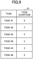
- Fig. 9 is a drawing illustrating an example of a task list.
- An example of jobList generated by the relaxed solution generation unit 22 is illustrated as a list 61.
- the list 61 of this example includes 6 tasks which are arranged from the top in the following order: the task #1, the task #2, the task #3, the task #4, the task #5, and the task #6.
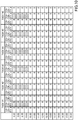
- Fig. 10 is a drawing illustrating an example of the initial state of a model defining a resource-constrained project scheduling problem.
- the resource-constrained project scheduling problem illustrated in Fig. 10 is the problem in which the six tasks #1 through #6 are allocated to the three facilities 1 through 3, with the time range subjected to scheduling being from the time slot at 8:30 to the time slot at 15:30.
- the time periods highlighted in dot shading indicate the periods during which the indicated facilities cannot be used.
- the relaxed solution generation unit 22 is expected to allocate the six tasks included in the list 61 of Fig. 9 to the resources (i.e., facilities) in the model defined in Fig. 10 .
- step S22 of Fig. 8 the relaxed solution generation unit 22 removes a task from the top of jobList, followed by designating the removed task as targetJob.
- the task stored at the top of the list 61 is the task #1, so that this task #1 is removed and designated as targetJob.
- step S23 the relaxed solution generation unit 22 selects a resource having the earliest task unallocated time T, and designates the selected resource as "resource".
- the process in step S23 may select arbitrary facility, e.g., the facility 1, and may designate this selected facility as "resource”.
- step S24 of Fig. 8 the relaxed solution generation unit 22 allocate targetJob to "resource” such that targetJob starts at the earliest task unallocated time T in "resource".
- allocation is performed by disregarding constraints (e.g., the constraint requiring that a task is allocated only to the facility usable time).
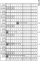
- Fig. 11 is a drawing illustrating the state of the model defining a resource-constrained project scheduling problem as observed after allocating one task.
- the task #1 is allocated to the facility 1 such as to start at 8:30 that is the earliest time to which no task is allocated in the facility 1.
- the state is such that the task #1 is allocated to the position indicated by an arrow 71.
- step S25 the relaxed solution generation unit 22 checks whether the number of elements in jobList is zero. When the number of elements is not zero, the procedure by the relaxed solution generation unit 22 returns to step S22.
- step S22 The top of jobList existing at the time of return to step S22 is the task #2, so that the relaxed solution generation unit 22 removes the task #2 as targetJob. Steps S23 and S24 are then performed, which causes the relaxed solution generation unit 22 to allocate the task #2 to the facility 2.
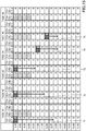
- the current state following the state illustrated in Fig. 11 is as illustrated in Fig. 12 in which the task #2 is allocated as indicated by an arrow 72.
- the task #2 is allocated to the facility 2 at the unusable time by disregarding the period during which the facility 2 is unusable (i.e., the period highlighted in dot shading). The procedure thereafter returns to step S22 again.
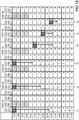
- step S22 The top of jobList existing at the time of return to step S22 is the task #3, so that the relaxed solution generation unit 22 removes the task #3 as targetJob. Steps S23 and S24 are then performed, which causes the relaxed solution generation unit 22 to allocate the task #3 to the facility 3 as indicated by an arrow 73 in Fig. 13 . The procedure thereafter returns to step S22 again.
- Steps S22 through S24 are performed again, which causes the relaxed solution generation unit 22 to allocate the task #4 to the facility 3 as indicated by an arrow 74 in Fig. 14 .
- the facility 3 has the earliest task unallocated time among the facilities 1 through 3, so that the facility 3 is designated as "resource" in step S23, and the facility 3 is selected as the place of allocation for the task #4.
- steps S22 through S24 are performed again, which causes the relaxed solution generation unit 22 to allocate the task #5 to the facility 2 as indicated by an arrow 75 in Fig. 15 .
- steps S22 through S24 are performed again, which causes the relaxed solution generation unit 22 to allocate the task #6 to the facility 1 as indicated by an arrow 76 in Fig. 16 .
- step S25 it is determined in step S25 that the number of elements in jobList is zero, which brings the relaxed-solution generation process of the relaxed solution generation unit 22 to an end.
- the relaxed solution generation unit 22 allocates tasks to resources by using a deterministic algorithm by disregarding constraints, thereby providing a solution violating a constraint that will be used as the initial value of the relaxed-solution data 20C.
- an approximate solution of a makespan minimization problem is obtained with high accuracy in a short time in the resource-constraint project scheduling problem.
Landscapes
- Engineering & Computer Science (AREA)
- Business, Economics & Management (AREA)
- Human Resources & Organizations (AREA)
- Theoretical Computer Science (AREA)
- Economics (AREA)
- Strategic Management (AREA)
- Entrepreneurship & Innovation (AREA)
- General Physics & Mathematics (AREA)
- Physics & Mathematics (AREA)
- Tourism & Hospitality (AREA)
- Development Economics (AREA)
- Quality & Reliability (AREA)
- Marketing (AREA)
- Game Theory and Decision Science (AREA)
- General Business, Economics & Management (AREA)
- Operations Research (AREA)
- Software Systems (AREA)
- Educational Administration (AREA)
- General Engineering & Computer Science (AREA)
- Life Sciences & Earth Sciences (AREA)
- Biodiversity & Conservation Biology (AREA)
- Computing Systems (AREA)
- Management, Administration, Business Operations System, And Electronic Commerce (AREA)
- Complex Calculations (AREA)
Abstract
Description
- The disclosures herein relate to an optimization apparatus, an optimization method, and an optimization program.
- The resource-constrained project scheduling problem is a problem in combinatorial optimization. The resource-constrained project scheduling problem concerns a situation in which constrains are imposed on a plurality of tasks and a plurality of resources, and requires the plurality of resources to be allocated to the plurality of tasks while satisfying the constraints such that the duration of the project is shorter than a target optimization period. An example of an objective function used in the resource-constrained project scheduling problem is a project completion time (i.e., the time at which all the tasks are completed). The problem that minimizes the makespan is referred to as a makespan minimization problem.
- Accordingly, there may be a need to provide a method of obtaining an approximate solution of a makespan minimization problem with high accuracy in a short time in the resource-constraint project scheduling problem.
-
- [Patent Document 1] Japanese Laid-open Patent Publication No.
2018-185639 - [Patent Document 2] Japanese Patent Laid-open Publication No.
11-195066 - According to an aspect of the embodiment, an optimization apparatus for repeatedly obtaining a constraint violating solution, a constraint satisfying solution, and an approximate solution in a resource-constrained project scheduling problem includes a memory and one or more arithmetic circuits coupled to the memory and configured to perform setting an end time of a target optimization period at a point between a first finish time that is equal to a finish time of a latest version of the constraint violating solution and a second finish time that is equal to a finish time of a latest version of the constraint satisfying solution, followed by obtaining the approximate solution by use of a metaheuristic algorithm, making a determination as to whether the approximate solution violates constraint or satisfy the constraint, and performing, based on the determination, updating the first finish time with a finish time of the approximate solution when the approximate solution violates the constraint, and updating the second finish time with a finish time of the approximate solution when the approximate solution satisfies the constraint, wherein the approximate solution is repeatedly obtained while updating the first finish time and the second finish time.
-
-
Fig. 1 is a drawing illustrating an example of the hardware configuration of an optimization apparatus for executing an optimization method; -
Fig. 2 is a drawing illustrating an example of the functional configuration of the optimization apparatus; -
Fig. 3 is a drawing schematically illustrating an example of a resource-constrained project scheduling problem; -
Fig. 4 is a drawing illustrating an example of a binary-variable-based model of the resource-constrained project scheduling problem illustrated inFig. 3 ; -
Fig. 5 is a drawing illustrating an example of input data that is used in an optimization process and that is generated based on a relaxed solution and a best solution; -
Fig. 6 is a drawing illustrating the updating of either one of relaxed-solution data and best solution data by use of data indicative of a generated approximate solution; -
Fig. 7 is a flowchart illustrating an example of the procedure of an approximation method; -
Fig. 8 is a flowchart illustrating an example of the procedure of generating a relaxed solution; -
Fig. 9 is a drawing illustrating an example of a task list; -
Fig. 10 is a drawing illustrating an example of the initial state of a model defining a resource-constrained project scheduling problem; -
Fig. 11 is a drawing illustrating the state of the model defining a resource-constrained project scheduling problem as observed after allocating one task; -
Fig. 12 is a drawing illustrating the state of the model defining a resource-constrained project scheduling problem as observed after allocating two tasks; -
Fig. 13 is a drawing illustrating the state of the model defining a resource-constrained project scheduling problem as observed after allocating three tasks; -
Fig. 14 is a drawing illustrating the state of the model defining a resource-constrained project scheduling problem as observed after allocating four tasks; -
Fig. 15 is a drawing illustrating the state of the model defining a resource-constrained project scheduling problem as observed after allocating five tasks; and -
Fig. 16 is a drawing illustrating the state of the model defining a resource-constrained project scheduling problem as observed after allocating six tasks. - In combinatorial optimization problems such as a resource-constraint project scheduling problem, an increase in the number of dimensions of search space results in an explosive increase in the number of combinations of variables. In such a case, the use of exhaustive search, which calculates all possible combinations, requires lengthy computational time that is practically infeasible. Instead of finding the true optimum solution, thus, a general-purpose approximation algorithm (i.e., metaheuristic algorithm) based on a heuristic approach may be used, or an approximation algorithm that obtains a good approximate solution within a practically feasible computational time may be used.
- A metaheuristic algorithm can obtain an optimum solution or a solution sufficiently close to the optimum solution, if given a sufficiently long computational time, through state transitions starting from an initial state to search for solutions attaining successively smaller values of an objective function. However, a solution that is sufficiently close to the optimal solution is not always readily obtained within a practically feasible computational time.
- Examples of an apparatus for performing simulated annealing, which is one type of metaheuristic algorithm, include an Ising machine (i.e., Boltzmann machine) using an Ising energy function. In Ising machine, the problem to be solved is represented as an Ising model using binary variables. In order to allow an Ising machine to obtain an approximate solution by formulating a model representing a resource-constrained project scheduling problem, various constraints regarding a plurality of tasks and a plurality of resources may be incorporated into an objective function, and, then, the objective function may be minimized to obtain a solution. However, there is a problem in an Ising model in that it is difficult to directly formulate a makespan minimization problem.
- One type of method for incorporating a makespan minimization problem indirectly into an Ising model is a method of using auxiliary variables represented as binary variables. Namely, n binary variables yi (i=1 to n) are introduced, for example, and these n binary variables are used to represent a value C=y1+2y2+3y3+4y4+...+nyn, for example. Use of an Ising machine to minimize the value of the objective function C while satisfying the constraints "the completion time of all tasks < C" and "only one of yi is 1" allows an approximate solution to be obtained in a makespan minimization problem. Use of this method, however, entails an increase by n in the number of dimensions of the search space in combinatorial optimization, resulting in a significant decrease in the performance of the Ising model for obtaining a solution.
- As an alternative, a makespan minimization problem may be represented by a different problem as an approximation thereto, thereby allowing a solution to be obtained that is approximate to the solution of the makespan minimization problem. For example, the durations of all the individual tasks are added to obtain a sum, and an Ising machine is used to obtain an approximate solution such as to minimize the sum serving as an objective function. It may be noted, however, that the sum may vastly differ, even when the makespans are almost the same, between the case in which all the tasks are completed substantially at the same time and the case in which one task is completed significantly later than the other tasks. As is understood from the above, methods of using a different problem as an approximation to a makespan minimization problem cannot produce a highly accurate approximate solution.
- Accordingly, there may be a need for a method of obtaining an approximate solution of a makespan minimization problem with high accuracy in a short time in the resource-constraint project scheduling problem.
- In the following, embodiments of the invention will be described with reference to the accompanying drawings.
-
Fig. 1 is a drawing illustrating an example of the hardware configuration of an optimization apparatus for executing an optimization method. The optimization apparatus illustrated inFig. 1 includes aCPU 11, adisplay unit 12, aninput unit 13, aROM 14, aRAM 15, anHDD 16, anetwork interface 17, a removable-memory-medium drive 18, and ametaheuristic calculation unit 19. TheCPU 11 and themetaheuristic calculation unit 19 are arithmetic circuits. - The
input unit 13 provides user interface, and receives various commands for operating the optimization apparatus and user responses responding to data requests or the like. Thedisplay unit 12 displays the results of processing by the optimization apparatus, and further displays various data that make it possible for a user to communicate with the optimization apparatus. Thenetwork interface 17 is used to communicates with peripheral devices and with remote locations. - The optimization apparatus illustrated in
Fig. 1 is a computer, and the optimization method is provided as a computer program executable by the optimization apparatus. This computer program is stored in a memory medium M that is mountable to the removable-memory-medium drive 18. The computer program is loaded to theRAM 15 or to theHDD 16 from the memory medium M through the removable-memory-medium drive 18. Alternatively, the computer program may be stored in a memory medium (not shown) provided in a peripheral apparatus or at a remote location, and is loaded to theRAM 15 or to theHDD 16 from the memory medium through thenetwork interface 17. - Upon receiving user instruction for program execution from the
input unit 13, theCPU 11 loads the program to theRAM 15 from the memory medium M, the peripheral apparatus, the remote memory medium, or theHDD 16. TheCPU 11 executes the program loaded to theRAM 15 by use of an available memory space of theRAM 15 as a work area, and continues processing while communicating with the user as such a need arises. TheROM 14 stores control programs for the purpose of controlling basic operations of the CPU 48 or the like. - By executing the computer program as described above, the optimization apparatus performs the function to obtain an approximate solution to a makespan minimization problem. The
metaheuristic calculation unit 19 may be a dedicated hardware specifically designed to execute a metaheuristic algorithm, and may be a dedicated hardware that performs simulated annealing to search for a solution of an Ising problem. In an alternative configuration, themetaheuristic calculation unit 19 may not be provided. In such a case, theCPU 11, which is the processor of a general-purpose computer, functions as a metaheuristic calculation unit to perform a metaheuristic algorithm. The metaheuristic algorithm may be simulated annealing, a random walk search algorithm, a genetic algorithm, a stochastic evolution algorithm, taboo search, or the like. It suffices for a metaheuristic algorithm to search in a heuristic manner for a solution (i.e., approximate solution) approximate to the solution that minimizes an objective function. -
Fig. 2 is a drawing illustrating an example of the functional configuration of the optimization apparatus. The optimization apparatus illustrated inFig. 2 includes adata storage unit 20, adata acquisition unit 21, a relaxedsolution generation unit 22, an optimizationdata generation unit 23, ametaheuristic calculation unit 24, asolution check unit 25, asolution update unit 26, atermination check unit 27, and adata output unit 28. - The functional units other than the
data storage unit 20 and themetaheuristic calculation unit 24 may be implemented by theCPU 11 illustrated inFig. 1 . The function of thedata storage unit 20 may be implemented by theRAM 15 or theHDD 16 illustrated inFig. 1 . The function of themetaheuristic calculation unit 24 may be implemented by theCPU 11 or themetaheuristic calculation unit 19 illustrated inFig. 1 . - It may be noted that boundaries between functional blocks illustrated as boxes indicate functional boundaries, and may not necessarily correspond to boundaries between program modules or separation in terms of control logic. One functional block and another functional block may be combined into one functional block that functions as one block. One functional block may be divided into a plurality of functional blocks that operate in coordination.
- The
data storage unit 20 stores therein a task information database (task information DB) 20A, a resource information database (resource information DB) 20B, relaxed-solution data 20C, andbest solution data 20D. - The
data acquisition unit 21 stores, in thetask information database 20A and theresource information database 20B, data regarding individual tasks and data regarding individual resources that are supplied from an external source to define a resource-constrained project scheduling problem. Data regarding constraints on the individual tasks and the individual resources may also be stored in thetask information database 20A and theresource information database 20B. -
Fig. 3 is a drawing schematically illustrating an example of a resource-constrained project scheduling problem. The resource-constrained project scheduling problem illustrated inFig. 3 is defined such thattasks # 1 through #3 for each of the products A and B andtasks # 1 and #2 for a product C are allocated to fourfacilities 1 through 4. A makespan minimization problem in this resource-constrained project scheduling problem is the problem that requires all the tasks to be scheduled such as to make as early as possible a project completion time Tms (i.e., the completion time of the last task completed). - In a resource-constrained project scheduling problem, various constraints may be imposed on a plurality of tasks and a plurality of resources. In the example illustrated in
Fig. 3 , for example, a time period indicated as "UNUSABLE" refers to the time period in which the indicated facility cannot be used to perform a task. In this manner, constrains may be imposed on resource usable time. Further, as constrains on the order of tasks, constraints may be imposed such thattasks # 1, #2, and #3 for a given product may need to be performed in the order named, without overlapping one another in time. Moreover, constraints may be imposed on correspondence between tasks and resources such as the requirement that a particular task can only be performed by a particular resource, and constraints may be imposed on the allowable start time and the required completion time of individual tasks. -
Fig. 4 is a drawing illustrating an example of a binary-variable-based model of the resource-constrained project scheduling problem illustrated inFig. 3 . In order for themetaheuristic calculation unit 24 illustrated inFig. 2 to function as an Ising machine to perform an optimization process formulated as an Ising model, the resource-constrained project scheduling problem is formulated as a binary-variable-based model, on which an optimization process is performed. The binary-variable-based model as illustrated inFig. 4 is not only applicable to an optimization process performed by an Ising machine, but also applicable to an optimization process performed by a different metaheuristic algorithm. - In order to formulate a binary-variable-based model of the resource-constrained project scheduling problem illustrated in
Fig. 3 , binary variables xjmt may be defined. Subscript j identifies a task, subscript m identifying a resource, and subscript t identifying a time. For example, thetask # 1 for the product A is identified by a task j=1, allocation to thefacility 1 identified by a resource m=1, and the time 8:30 identified by atime slot number 1. The fact that the value of xjmt becomes 1 for j=1, m=1, and t=1 (namely, x111=1) represents the fact that thetask # 1 for the product A starts at the time 8:30 by use of thefacility 1. - Each row of the table illustrated in
Fig. 4 represents time (by time slots in units of 30 minutes), and each column represents a combination between a task and a facility. For example, acolumn 31 shows a value, at a time t, of a variable x11t which defines the fact that thetask # 1 for the product A is allocated to thefacility 1. Thetask # 1 for the product A starts at the time 8:30 by use of thefacility 1, so that the value of x11t assumes "1" only in the time slot corresponding to the time 8:30 (i.e., x111=1), and assumes "0" in any other time slots. - As the value of a task j, the task #k for the product A may be identified by a task j=k, the task #k for the product B being identified by a task j=3+k, and the task #k for the product C being identified by a task j+6+k. For example, the variable for representing the fact that the
task # 2 for the product B is allocated to thefacility 1 is x51t. With this arrangement, the columns illustrated inFig. 4 correspond, from left to right, the following variables: x11t, x12t, x13t, x14t, x21t, x22t, x23t, x24t, x31t, x32t, x33t, x34t, x41t, x42t, x43t, x44t, x51t, x52t, x53t, ..., x74t, x81t, x82t, x83t, x84t. Variable x51t corresponds to the column 32, and assumes a value of "1" only at the time 10:30, which represents the fact that thetask # 2 for the product B starts at the time 10:30 by use of thefacility 1. It may be noted that the time slot corresponding to the time 10:30 is the fifth time slot identified by a time t=5, so that x515=1. - The length of time required to complete each task (i.e., the required time) is not defined by the value of variable xjmt. Instead, a constant for representing the required time of each task is defined separately. As will be described later, this constant is used to manipulate subscript t, thereby allowing conditions regarding the require time to be specified.
- In the following, a description will be given of an example of formulation of a resource-constrained project scheduling problem by using binary variable xjmt described in the above example. In order to formulate a resource-constrained project scheduling problem, an objective function that is to be minimized in an optimization process performed by the
metaheuristic calculation unit 24 may be defined by binary variable xjmt. - In order to specify various constraints regarding binary variable xjmt, the following constants are defined.
- jtj: the number of time slots of the required time for task j
- jstj: the sequence number of the time slot of the allowable start time for task j
- jdtj: the sequence number of the time slot of the completion time for task j
- ck: Weight for constraint term Qk
- J: a set of tasks j
- M: a set of resources m
- T: a set of time slots subjected to optimization
- MTm: a set of time slots allocatable to a resource m (MTm ⊂ T)
- M_JOBm: a set of tasks executable by a resource m (M_JOBm ⊂ J)
- PRE: a set of combinations each comprised of a task jp, a task jn, and a waiting time wait (i.e., a set of combinations of tasks and a waiting time for which the start of the task jn occurs at the end of a time wait after the start of the task jp)
- Based on these constants and sets, an objective function E is formulated as a weighting sum of constraint terms Qk multiplied by respective weighting factors ck as follows.


- The constraint term Q1 defines the constraint that each task is started at or after the preset start time (wherein the start time of a task j is the time slot sequence number jstj). The sum is obtained of binary variables xjmt satisfying the condition that the start occurs prior to the time slot sequence number jstj, so that the value of the objective function E increases as a penalty when a value of xjmt subjected to the summation becomes 1.
- The constraint term Q2 defines the constraint that each task is completed by the preset completion time (wherein the completion time of a task j is the time slot sequence number jdtj). The sum is obtained of binary variables xjmt satisfying the condition that the start occurs after the time slot sequence number jdtj-jtj (i.e., completion time - required time = required start time), so that the value of the objective function E increases as a penalty when a value of xjmt subjected to the summation becomes 1.
- The constraint term Q3 defines the constraint that a resource is not used during the time outside the resource usable time (i.e., the time belonging to the complement of the set MTm constituted by time slots allocatable to the resource m). The sum of binary variables xjmt is obtained with respect to the time slot sequence numbers belonging to the complement of the set MTm constituted by time slots allocatable to the resource m, so that the value of the objective function E increases as a penalty when a value of xjmt subjected to the summation becomes 1.
- The constraint term Q4 defines the constraint that only the tasks allocatable to a resource (i.e., tasks belonging to the set M_JOBm constituted by tasks executable by a resource m) are allocated to such a resource. The sum of binary variables xjmt is obtained with respect to the tasks belonging to the complement of the set M_JOBm constituted by tasks executable by a resource m, so that the value of the objective function E increases as a penalty when a value of xjmt subjected to the summation becomes 1.
- The constraint term Q5 defines the constraint that each task is performed only once. The squared term included in the constraint term Q5 is the square of a number obtained by subtracting 1 from the sum that is obtained, with respect to all the resources m and all the time slots t, of binary variables xjmt specifying a particular task j. This squared term becomes 0 when the value of xjmt becomes 1 only once for all the resources m and all the time slots t. In other cases, the squared term assumes a value greater than 0, so that the value of the objective function E increases as a penalty.
- The constraint term Q6 defines the constraint that no resource has two or more tasks simultaneously allocated thereto. With respect to a given resource m, variable xjmt assumes a value of 1 when the task j starts at the time slot t, and variable xj'mt' assumes a value of 1 when another task j' starts during a period t' between the time slot t and the end of the required time jtj of the task j following the time slot t, which results in the product of these two variables becoming 1. With the sum of such products being incorporated into the objective function, allocating two or more tasks simultaneously to a given resource causes the value of the objective function E to increase as a penalty.
- The constraint term Q7 defines a constraint on the order of tasks such that a next task jn starts upon waiting for the time "wait" after a preceding task jp. Variable xjpmt assumes a value of 1 when the task jp starts at the time slot t by using the resource m, and variable xjnm't' assumes a value of 1 when the task jn starts at the time slot t' (=t+wait) equal to the end of the time "wait" following the time slot t by using the resource m', which results in the product of these two variables becoming 1. The value of such a product satisfying the above-noted condition is not incorporated as a penalty, but the sum of such products corresponding to other conditions is incorporated into the objective function. With this arrangement, the value of the objective function E increases when the constraints on the order of tasks are violated.
- When simulated annealing, for example, is used to obtain an approximate solution to the resource-constrained project scheduling problem formulated into the above-described model, a state S having binary variables xjmt as described above may be defined. An objective function value E of the current state S is calculated, and, then, an objective function value E' of the next state S' obtained by making a slight change (e.g., 1-bit inversion) from the current state S is calculated, followed by calculating a difference ΔE (= E'-E) between these two states. In the case in which the Boltzmann distribution is used to represent the probability distribution of S and the Metropolis method is used, for example, probability P with which a transition to the next state S' occurs may be defined by the following formula.

- Here, β is thermodynamic beta (i.e., the reciprocal of absolute temperature). The function min[1, x] assumes a value of 1 or a value of x, whichever is smaller. According to the above formula, a transition to the next state occurs with probability "1" in the case of ΔE≦0, and a transition to the next state occurs with probability exp(-βΔE) in the case of 0<ΔE.
- Lowering temperature at a sufficiently slow rate, while performing state transitions, allows the state to be converged, theoretically, on an optimum solution having the smallest objective function value. The Metropolis method is a non-limiting example, and other transition control algorithms such as Gibbs sampling may alternatively be used.
- In the manner described above, the resource-constrained project scheduling problem is formulated into a binary-variable-based model. The
task information database 20A and theresource information database 20B stored in thedata storage unit 20 illustrated inFig. 2 may include data indicative of variables xjmt, the constants, the sets, the objective function, and the like for defining the model as described above. - Referring to
Fig. 2 again, the relaxedsolution generation unit 22 generates a relaxed solution, i.e., a solution violating a constraint, based on the data indicative of tasks, the data indicative of resources, and the data indicative of constraints stored in thetask information database 20A and theresource information database 20B. The solution violating a constraint refers to a solution that does not satisfy at least part of the constraints imposed on the tasks and the resources. Such a solution is situated outside the search space satisfying the constraints, and is situated within a search space satisfying at least partially relaxed constraints. In the present application, the term "relaxed solution" and the term "solution violating a constraint" are used to refer to the same meaning. - The data indicative of a relaxed solution generated by the relaxed
solution generation unit 22 is stored as relaxed-solution data 20C in thedata storage unit 20. The relaxed-solution data 20C includes at least the data indicative of the finish time of a relaxed solution, i.e., the data indicative of the finish time of the task that is completed last among the tasks constituting the relaxed solution. - As an opposite to the solution violating a constraint, a solution satisfying constraints is further defined as a solution satisfying the conditions. The solution satisfying constraints may be a solution that satisfies all the constraints defined in an objective function while the solution violating a constraint may be a solution that does not satisfy part of the constraints defined in the objective function. As will be described later, data indicative of a solution satisfying constraints obtained by the
metaheuristic calculation unit 24 is stored asbest solution data 20D in thedata storage unit 20. In the present application, the term "solution satisfying constraints" and the term "best solution" are used to refer to the same meaning. Thebest solution data 20D includes at least the data indicative of the finish time of a solution satisfying constraints, i.e., the data indicative of the finish time of the task that is completed last among the tasks constituting the solution satisfying constraints. - It may be noted that when the solution satisfying constraints is defined as a solution that satisfies all the constraints defined in an objective function as described above, the case of the objective function E previously described requires that the solution satisfying constraints is the solution for which the value of the objective function E becomes the smallest value "zero". Alternatively, a solution that satisfies part of the constraints (e.g., some constraint terms among the constraint terms Q1 through Q7 previously described) may be defined as a solution satisfying constraints while a solution not satisfying such a part of the constraints may be defined as a solution violating a constraint. In this case, such a part of the constraints that should be satisfied by a solution satisfying constraints may be constraints that need to be satisfied or that are important, and may be defined in accordance with the configuration of the problem. For example, the condition that each task is performed only once and the condition that a resource is not used outside the usable time may be important. In such a case, a solution satisfying these two conditions (i.e., Q3=Q5=0) may be treated as a solution satisfying constraints while a solution not satisfying these conditions may be treated as a solution violating a constraint.
- The relaxed
solution generation unit 22 may generate a relaxed solution based on a metaheuristic algorithm. In so doing, a weighing factor ck may be set to zero with respect to one or more constraint terms that are part of the constraint terms Qk included in the objective function E previously described, for example, and that define one or more conditions other than part of the constraints (e.g., the constraint term Q5 requiring each task to be performed only once). An approximate solution may then be obtained by minimizing the objective function. With this arrangement, a solution violating a constraint may be obtained for which the constraint term Q3, for example, requiring a resource to be not used outside the resource usable time assumes a value greater than zero (i.e., the resource is used during the resource unusable time). - The relaxed
solution generation unit 22 may generate a relaxed solution by use of a deterministic algorithm, rather than by use of a metaheuristic algorithm. A metaheuristic algorithm, in general, is designed such that a probabilistic factor is used to gradually decrease an objective function value while satisfying constraints without being trapped at an unfavorable local solution, thereby generating a satisfactory solution. It suffices for the relaxedsolution generation unit 22 to generate a solution without any regard to the constraints. A deterministic algorithm that ignores the constraints may thus readily generate a relaxed solution. Use of a deterministic algorithm allows an initial value of a relaxed solution to be easily obtained in an efficient manner. - Based on the data stored in the
data storage unit 20, the optimizationdata generation unit 23 generates input data used in an optimization process performed by themetaheuristic calculation unit 24. The input data generated by the optimizationdata generation unit 23 includes the end time of a target optimization period which is used in the optimization process performed by themetaheuristic calculation unit 24. The end time of a target optimization period is equal to the sequence number of the last time slot belonging to the set T of time slots subjected to the optimization process, which is one of the constants described in connection with the model formulation of a resource-constrained project scheduling problem previously described. This time is obtained based on the relaxed-solution data 20C and thebest solution data 20D as will be described later. Specifically, the end time of a target optimization period is set between the finish time of a relaxed solution indicated by the relaxed-solution data 20C and the finish time of a best solution indicated by thebest solution data 20D. -
Fig. 5 is a drawing illustrating an example of input data that is used in an optimization process and that is generated based on a relaxed solution and a best solution. InFig. 5 , for the sake of convenience of explanation, only the data indicative of thetasks # 1 through #3 for the product A (i.e., the tasks A1 through A3) are illustrated, and the relaxed-solution data 20C and thebest solution data 20D are stored in thedata storage unit 20. - The relaxed-
solution data 20C specifies the state of a relaxed solution based on the model using binary variables xjmt previously described. Likewise, thebest solution data 20D specifies the state of a best solution based on the model using binary variables xjmt. InFig. 5 , the arrays of values of variables xjmt are illustrated by using a table format similar to that ofFig. 4 for the purpose of allowing the state of solutions to be visually recognized. In the tables illustrating the relaxed-solution data 20C and thebest solution data 20D, the time periods highlighted in dot shading indicate the periods during which the indicated resources cannot be used. - In the example illustrated in
Fig. 5 , a distinction between the solution satisfying constraints and the solution violating a constraint is made according to whether the constraint term Q3 previously described is satisfied, i.e., whether the indicated resources are used only during the resource usable time. In the table of the relaxed solution illustrated inFig. 5 , the time at which the task A3 (i.e., thetask # 3 for the product A) is started by using thefacility 3 is 10:00 at which thefacility 3 cannot be used. Namely, this relaxed solution is a solution violating a constraint for which the constraint term Q3 previously described has a value greater than zero (i.e., the resource is used during the resource unusable time). In the table of the best solution, scheduled tasks do not include any task that is performed during the resource unusable time, so that this solution satisfies the constraint represented by the constraint term Q3. Namely, this best solution is a solution satisfying constraints for which the constraint term Q3 previously described has a value of zero (i.e., the resource is used only during the resource usable time). - In
Fig. 5 , the finish time of the task that is completed last among the tasks included in the relaxed solution is the finish time T1 of the relaxed solution. Further, the finish time of the task that is completed last among the tasks included in the best solution is the finish time T2 of the best solution. In this example, the time slot sequence number of the finish time T1 is 9, and the time slot sequence number of the finish time T2 is 15. - As illustrated in
Fig. 5 , the optimizationdata generation unit 23 generatesinput data 41 for an optimization process based on the relaxed-solution data 20C and thebest solution data 20D stored in thedata storage unit 20. Theinput data 41 represents tasks, facilities, and time slots subjected to an optimization process based on the model using binary variables xjmt. Theinput data 41 defines the configuration of a problem in which scheduling is made to allocate tasks to facilities at particular time slots. InFig. 5 , the arrays of values of variables xjmt are illustrated by using a table format similar to that ofFig. 4 for the purpose of allowing the state of variables to be visually recognized. Theinput data 41 defines that an optimization process is to be performed such that three tasks are allocated to three facilities between the timeslot sequence number 0 at 8:30 and the timeslot sequence number 13 at 15:00. It may be noted that the set T of time slots subjected to an optimization process, as previously described, accordingly includes, as elements of the set, the time slots from 8:30 to 15:00. - The optimization
data generation unit 23 generates theinput data 41 such that the time of the last time slot of the input data 41 (i.e., the end time of a target optimization period) is situated between the finish time T1 of the relaxed solution and the finish time T2 of the best solution described above. In so doing, the interval between the finish time T1 and the finish time T2 may be divided with a predetermined ratio (e.g., 1:1), so that the end time of a target optimization period is set at the point of the divide. Setting the end time of a target optimization period according to a predetermined ratio allows a simple process to generate theinput data 41 in an efficient manner. Based on theinput data 41 generated as described above, themetaheuristic calculation unit 24 performs an optimization process as will be described below. - By referring to
Fig. 2 again, themetaheuristic calculation unit 24 performs a heuristic optimization process based on the data configured by the optimizationdata generation unit 23, thereby generating an approximate solution that minimizes the value of a designed objective function. In performing an optimization process, tasks are scheduled such that the finish time of any given task is no later than the end time of a target optimization period set by the optimizationdata generation unit 23. Namely, when the end time of a target optimization period is set to the time slot at 15:00, for example, the optimization process evaluates only those schedules in which all the tasks are completed before or at the time slot of 15:00. This is achieved by setting the last time slot of the set T of time slots subjected to an optimization process to the end time of a target optimization period. An approximate solution generated by themetaheuristic calculation unit 24 may sometimes be a solution violating a constraint and may sometimes be a solution satisfying constraints, depending on various conditions including the end time of a target optimization period. - A solution violating a constraint or a solution satisfying constraints generated by the
metaheuristic calculation unit 24 are used by thesolution update unit 26 to update the relaxed-solution data 20C or thebest solution data 20D, as will be described later in detail. Specifically, thesolution update unit 26 replaces the relaxed-solution data 20C with the data indicative of a solution violating a constraint upon the occurrence of a solution violating a constraint, and replaces thebest solution data 20D with the data indicative of a solution satisfying constraints upon the occurrence of a solution satisfying constraints. In this manner, the calculation of an approximate solution by the optimization process of themetaheuristic calculation unit 24 and the updating of the relaxed-solution data 20C and thebest solution data 20D by thesolution update unit 26 are repeatedly performed, thereby successively updating solutions. - In the following, the updating of solutions described above will be described in more detail.
- The optimization
data generation unit 23 and themetaheuristic calculation unit 24 function as anoptimization process unit 30. Theoptimization process unit 30 performs an optimization process in a resource-constrained project scheduling problem to generate an approximate solution based on thetask information database 20A, theresource information database 20B, relaxed-solution data 20C, and thebest solution data 20D. Specifically, theoptimization process unit 30 sets the end time of a target optimization period at a point between the first finish time that is the finish time of a preceding solution violating a constraint and the second finish time that is the finish time of a preceding solution satisfying constraints, followed by obtaining an approximate solution by use of a metaheuristic algorithm. Namely, theoptimization process unit 30 sets the end time of a target optimization period at a point between the finish time (i.e., the first finish time) of a solution indicated by the latest relaxed-solution data 20C and the finish time (i.e., the second finish time) of a solution indicated by the latestbest solution data 20D, followed by obtaining an approximate solution by use of a metaheuristic algorithm. - Here, the term "approximate solution" refers to a solution that does not guarantee the occurrence of the minimum value of an objective function for optimization, and that can be regarded as a proper approximation to the optimum solution minimizing the objective function. In order for the
optimization process unit 30 to obtain an approximate solution, the optimization process makes successive state transitions in the search space such as to stochastically decrease the value of the objective function. Upon making transitions a predetermined number of times determined in advance, the state observed at that instance may be output as an approximate solution. Alternatively, theoptimization process unit 30 may perform the optimization process for a predetermined duration determined in advance, and, then, may output the state observed at that instance as an approximate solution. Alternatively, theoptimization process unit 30 may detect the event in which the value of an optimization process becomes lower than or equal to a predetermined value determined in advance, and, then, may output the state observed at that instance as an approximate solution. - When the optimization process performed based on the finish time of the relaxed-
solution data 20C and the finish time of thebest solution data 20D is performed for the first time, respective initial value data are used as the finish time of the relaxed-solution data 20C and the finish time of thebest solution data 20D. An initial value serving as the first relaxed-solution data 20C is the relaxed-solution data 20C generated by the relaxedsolution generation unit 22 as previously described. - In order to provide an initial value for the
best solution data 20D, theoptimization process unit 30 may generate a solution satisfying constraints. When providing an initial value for the best solution, the end time of a target optimization period may be set to a sufficiently large value (i.e., a sufficiently late point in time) that is feasible and sensible from the viewpoint of making a time schedule for tasks. In the optimization process, further, weighting factors for relevant constraints included in an objective function for optimization may be set to sufficiently large values, thereby ensuring that a solution satisfying constraints is sure to be obtained. Alternatively, the solution search space used in the optimization process may be limited to the space that satisfies constraints, so that state transitions made in the optimization process may be allowed only when the next state satisfy the constraints. Data indicative of the solution satisfying constraints generated first by theoptimization process unit 30 is stored as the initial value data of thebest solution data 20D in thedata storage unit 20. - When the
optimization process unit 30 generates an approximate solution as part of the solution updating process, thesolution check unit 25 determines whether the approximate solution generated by theoptimization process unit 30 is a solution violating a constraint or a solution satisfying constraints. In doing so, thesolution check unit 25 may determine that a solution satisfying all the constraints (e.g., all the constraint terms Q1 through Q7 previously described) is a solution satisfying constraints, and may determine that a solution not satisfying at least some of the constraints is a solution violating a constraint. Alternatively, thesolution check unit 25 may determine that an approximate solution satisfying predetermined constraints among a plurality of constraints is a solution satisfying constraints, and may determine that an approximate solution not satisfying these predetermined constraints is a solution violating a constraint. More specifically, thesolution check unit 25 may determine that a solution satisfying predetermined constraint terms among the constraint terms Q1 through Q7 previously described is a solution satisfying constraints, and may determine that a solution not satisfying at least some of these predetermined constraint terms is a solution violating a constraint. - Determining the type of solution in response to whether predetermined constraints are satisfied or not achieves proper solution determination that is responsive to the configuration of a problem and that reflects the importance or the like of individual constraints, thereby achieving an efficient solution search process for a makespan minimization problem. In general, when the end time of a target optimization period set by the optimization
data generation unit 23 is early, an obtained approximate solution is likely to be a solution violating a constraint. When the end time of a target optimization period set by the optimizationdata generation unit 23 is late, an obtained approximate solution is likely to be a solution satisfying constraints. - Based on the determination made by the
solution check unit 25, thesolution update unit 26 updates the first finish time by using the finish time of the approximate solution when the approximate solution is a solution violating a constraint, and updates the second finish time by using the finish time of the approximate solution when the approximate solution is a solution satisfying constraints. Namely, in the case in which the approximate solution generated by theoptimization process unit 30 is a solution violating a constraint, data of the approximate solution is used to update (i.e., replaces) the relaxed-solution data 20C (including the data indicative of the finish time of a solution) stored in thedata storage unit 20. Further, in the case in which the approximate solution generated by theoptimization process unit 30 is a solution satisfying constraints, data of the approximate solution is used to update (i.e., replaces) thebest solution data 20D (including the data indicative of the finish time of a solution) stored in thedata storage unit 20. -
Fig. 6 is a drawing illustrating the updating of either one of relaxed-solution data and best solution data by use of data indicative of a generated approximate solution. InFig. 6 , the same or corresponding elements as those ofFig. 5 are referred to by the same or corresponding numerals, and a description thereof will be omitted as appropriate. - Based on the
input data 41 generated by the optimizationdata generation unit 23 as described in connection withFig. 5 , themetaheuristic calculation unit 24 performs an optimization process to generate an approximate solution. In the example illustrated inFig. 6 , anapproximate solution 51 obtained by themetaheuristic calculation unit 24 indicates that all the tasks are performed during the resource usable time. In this case, thesolution check unit 25 may determine that the obtainedapproximate solution 51 is a solution satisfying constraints (i.e., best solution). - Based on this determination, the
solution update unit 26 replaces thebest solution data 20D stored in thedata storage unit 20 with the data indicative of the obtainedapproximate solution 51. In the example illustrated inFig. 6 , thebest solution data 20D in thedata storage unit 20 is updated, so that the finish time T2 of the best solution is changed from the timeslot sequence number 15 to the timeslot sequence number 11. - As described above, the optimization apparatus illustrated in
Fig. 2 successively updates the finish time (i.e., the first finish time) of a solution indicated by the relaxed-solution data 20C and the finish time (i.e., the second finish time) of a solution indicated by thebest solution data 20D, and causes themetaheuristic calculation unit 24 to produce an approximate solution repeatedly while performing such updating. Through this process, the finish time (i.e., the first finish time) of a solution indicated by the relaxed-solution data 20C and the finish time (i.e., the second finish time) of a solution indicated by thebest solution data 20D gradually approach each other. - The
termination check unit 27 checks whether a difference between the finish time (i.e., the first finish time) of a solution indicated by the relaxed-solution data 20C and the finish time (i.e., the second finish time) of a solution indicated by thebest solution data 20D becomes less than or equal to a predetermined value. When the difference in time becomes less than or equal to the predetermined value, i.e., when the first finish time and the second finish time become sufficiently close to each other or equal to each other, thetermination check unit 27 terminates the process of obtaining a solution approximate to the makespan minimum solution performed by the optimization apparatus. The solution indicated by thebest solution data 20D at the time the two finish times become equal or substantially equal to each other is consequently a proper approximate solution for the makespan minimum solution. Alternatively, thetermination check unit 27 may check whether a difference between the second finish time and the end time of a target optimization period becomes less than or equal to a predetermined value, and may terminate the process of obtaining a solution approximate to the makespan minimum solution based on such a check result. - In the following, a further description will be given of the operation in which the first finish time and the second finish time approach each other as described above.
- The first finish time is denoted as T1, and the second finish time is denoted as T2, with the makespan minimum solution (i.e., ideal solution) being denoted as TIDEAL. T1 is equal to the finish time of a solution when it is not possible (or is difficult) to obtain a solution satisfying constraints. T2 is equal to the finish time of a solution when a solution satisfying constraints is successfully obtained. The condition of T1 < T2 is thus satisfied with high probability. With the end time of a target optimization period being denoted as TEND, the condition of TEND < T2 is satisfied because TEND is set between T1 and T2. The finish time of an approximate solution to update T2 is always earlier than TEND, so that T2 is always updated to an earlier time whenever it is updated. Accordingly, T2 monotonously decreases (i.e., gradually moves to earlier time with certainty). The makespan minimum solution is the solution that has the earliest finish time among all the possible solutions satisfying constraints, so that the condition of TIDEAL ≤ T2 is satisfied. Since T2 is selected from the finish times of all the solutions satisfying constraints such as to monotonously decrease, T2 approaches TIDEAL promptly with certainty. When T2 becomes substantially equal to T1, the value of T2 is consequently a highly accurate approximate value for TIDEAL.
- It may be noted that the case in which a later one of T1 and T2 is T1, i.e., T2 < T1, can occur with low probability. Even in consideration of such a case, TEND is always earlier than TLATTER that is a later one of T1 and T2. Namely, the condition of TEND < TLATTER is satisfied. The finish time of an approximate solution to update T1 and T2 is always earlier than TEND, so that TLATTER is always updated to an earlier time whenever it is updated. Accordingly, a greater one (i.e., later one) of T1 and T2 monotonously decreases (i.e., gradually moves to earlier time with certainty). Namely, T2 also monotonously decreases with high probability. As is understood from the above, even when taking into account the case in which T2<T1 occurs with some probability, T2 approaches TIDEAL promptly with substantial certainty similarly to the manner previously described. When T2 becomes substantially equal to T1, the value of T2 is consequently a highly accurate approximate value for TIDEAL.
- The
data output unit 28 outputs data indicative of a solution that is obtained in the manner described above and that is approximate to the makespan minimum solution. The output data may be supplied to a display screen via thedisplay unit 12 illustrated inFig. 1 , to theHDD 16, to the memory medium M via the removable-memory-medium drive 18, or to an external device via thenetwork interface 17. - As described above, the optimization apparatus illustrated in
Fig. 2 successively updates the finish time of a solution indicated by the relaxed-solution data 20C and the finish time of a solution indicated by thebest solution data 20D, and causes a metaheuristic optimization process to produce an approximate solution repeatedly while performing such updating. As a feature of this optimization apparatus, the objective function subjected to minimization in the metaheuristic optimization process does not include a term whose value decreases as the makespan (i.e., the project completion time) becomes earlier and earlier. - It is difficult to incorporate an index for evaluating a makespan directly into an objective function. Because of this, a makespan evaluation index in the related art is incorporated indirectly, or as an approximation, into an objective function, followed by performing a metaheuristic optimization process to obtain a solution approximate to the makespan minimum solution. In contrast, the optimization apparatus illustrated in
Fig. 2 does not use a makespan evaluation index incorporated indirectly, or as an approximation, into the objective function. In the optimization process for one round of repeated process, thus, no mechanism whatsoever for decreasing a makespan is incorporated. - For one round of a metaheuristic optimization process, the optimization apparatus illustrated in
Fig. 2 does not evaluate a makespan, and obtains an approximate solution for a given end time of a target optimization period which minimizes the objective function that defines constraints. Then, based on the approximate solution obtained by the current-round optimization process, the end time of a target optimization period is shifted in the direction where a solution approximate to the makespan minimum solution is situated or is likely situated, and, then, a next-round optimization process is performed with respect to the shifted end time of a target optimization period. The shifting and updating of an end time of a target optimization period as described above allows an approximate solution obtained by an optimization process to move closer to a solution approximate to the makespan minimum solution. - As described above, the optimization apparatus illustrated in
Fig. 2 does not need to incorporate a makespan evaluation index for a resource-constrained project scheduling problem indirectly, or as an approximation, into the objective function, thereby avoiding the lowering of efficiency of a metaheuristic optimization process and the lowering of accuracy of a solution. Further, the end time of a target optimization period is shifted by the procedure similar to binary search. When the total number of time slots is N, therefore, performing an optimization process a number of times approximately equal to Log2N enables the obtainment of a proper approximate solution for makespan minimization. -
Fig. 7 is a flowchart illustrating an example of the procedure of an approximation method. The approximation method illustrated inFig. 7 may be performed by the function units illustrated inFig. 2 by use of the hardware illustrated inFig. 1 . - It may be noted that, in
Fig. 7 and the subsequent flowcharts, an order in which the steps illustrated in the flowchart are performed is only an example. The scope of the disclosed technology is not limited to the disclosed order. For example, a description may explain that an A step is performed before a B step is performed. Despite such a description, it may be physically and logically possible to perform the B step before the A step while it is possible to perform the A step before the B step. In such a case, all the consequences that affect the outcomes of the flowchart may be the same regardless of which step is performed first. It then follows that, for the purposes of the disclosed technology, it is apparent that the B step can be performed before the A step is performed. Despite the explanation that the A step is performed before the B step, such a description is not intended to place the obvious case as described above outside the scope of the disclosed technology. Such an obvious case inevitably falls within the scope of the technology intended by this disclosure. - In step S1, the
data acquisition unit 21 receives input data inclusive of resource information, task information, time information, and the like. The data received by thedata acquisition unit 21 is stored in thedata storage unit 20. - In step S2, the relaxed
solution generation unit 22 derives a solution by allocating resources to tasks by disregarding constraint violation, followed by storing data indicative of the derived solution as the relaxed-solution data 20C in thedata storage unit 20. In so doing, the relaxedsolution generation unit 22 may use a deterministic algorithm to allocate resources to tasks. - In step S3, the
metaheuristic calculation unit 24 derives a solution satisfying constraints by use of an Ising machine, for example, followed by storing data indicative of the derived solution as thebest solution data 20D in thedata storage unit 20. - In step S4, the optimization
data generation unit 23 sets the finish time T1 to the task completion time of a solution indicated by the relaxed-solution data 20C, and sets C1 to the amount of constraint violation of the solution indicated by the relaxed-solution data 20C. Here, the amount of constraint violation is a value indicative of the degree to which a solution violating a constraint violates constraints. In the optimization method illustrated inFig. 7 , the end time of a target optimization period is not set at the point in time at which the interval between the first finish time and the second finish time is divided with a predetermined ratio, but is set based on the amount of constraint violation and the amount of constraint conformity margin, which will be described later. - The amount of constraint violation may be the total number of time slots at which constraint is violated by the combination of a task and a resource (i.e., facility) in a relaxed solution, for example. Specifically, the constraint requiring that a task is allocated to a resource only during the resource usable time may be taken into consideration, for example. Then, the number of time slots at which such a constraint is violated by allocation is used as the amount of constraint violation. In the case of the relaxed solution indicated by the relaxed-
solution data 20C illustrated inFig. 5 , for example, the task A3 is allocated to thefacility 3 at the time slot sequence numbers "3" and "4" (i.e., 10:00 and 10:30)) which are resource unusable time. In the case of this relaxed-solution data, thus, the amount of constraint violation may be 2. - In step S5, the optimization
data generation unit 23 sets the finish time T2 to the task completion time of a solution indicated by thebest solution data 20D, and sets C2 to the amount of constraint conformity margin of the solution indicated by thebest solution data 20D. Here, the amount of constraint conformity margin is a value indicative of the degree to how much margin exists for a solution satisfying constraints to satisfy constraints. - The amount of constraint conformity margin may be the total number of time slots that are unallocated and usable in a best solution and that are counted over all the resources, for example. Specifically, the number of time slots that are unallocated and usable outside the resource unusable time may be obtained for each resource, and such numbers of time slots may be summed over all the resources. In the case of the best solution indicated by the
best solution data 20D illustrated inFig. 5 , for example, the number of time slots unallocated and usable for thefacility 1 is 15. Further, the number of time slots unallocated and usable for thefacility 2 is 10, and the number of time slots unallocated and usable for thefacility 3 is 7. In the case of this best solution data, thus, the amount of constraint conformity margin may be 32=15+10+7. - In step S6, the optimization
data generation unit 23 calculates the end time of a target optimization period based on the amount C1 of constraint violation and the amount C2 of constraint conformity margin, and rounds up the fraction as appropriate, followed by setting TEND to the obtained end time of a target optimization period. For example, the end time of a target optimization period may be set at a point in time that divides the interval between the first finish time T1 and the second finish time T2 according to the ratio corresponding to the amount C1 of constraint violation of a relaxed solution (i.e., an initial value or a preceding solution violating a constraint) and the amount C2 of constraint conformity margin of a best solution (i.e., an initial value of a preceding solution satisfying constraints). - More specifically, the end time TEND of a target optimization period may be calculated by use of the following formula, for example.

- Calculating the end time of a target optimization period in this manner allows the end time of a target optimization period to be set to a relatively late time (i.e., the time closer to T2 than to T1) when the amount C1 of constraint violation is relatively large, i.e., when the finish time T1 of a relaxed solution is situated at too early a time. Further, the end time of a target optimization period is set to a relatively early time (i.e., the time closer to T1 than to T2) when the amount C2 of constraint conformity margin is relatively large, i.e., when the finish time T2 of a best solution is so late as to provide a sufficient margin.
- Alternatively, the end time TEND of a target optimization period may be calculated by use of the following formula, for example.


- Setting the end time of a target optimization period based on the amount of constraint violation and the amount of constraint conformity margin allows time to be set in response to an index indicating that a relaxed solution is too early or that a best solution has too large a margin, thereby enabling efficient adjustment of the end time of a target optimization period. As a result, an approximate solution for makespan minimization is promptly obtained in a more efficient manner.
- In step S7, the
termination check unit 27 checks whether TEND and T2 equal to each other. Since the time indication given by the time slot sequence number is discrete, repeating the optimization process a sufficient number of times causes TEND to become eventually equal to T2. When TEND and T2 are not equal, the procedure proceeds to step S8. - In step S8, the
metaheuristic calculation unit 24 uses an Ising machine with respect to the end time TEND of a target optimization period to derive an approximate solution. In step S9, thesolution check unit 25 checks whether the derived solution is a solution violating a constraint. In the case of the derived solution being a solution violating a constraint, the procedure proceeds to step S10, in which thesolution update unit 26 stores data indicative of the derived solution in thedata storage unit 20 as the relaxed-solution data 20C. In the case of the derived solution being not a solution violating a constraint, the procedure proceeds to step S11, in which thesolution update unit 26 stores data indicative of the derived solution in thedata storage unit 20 as thebest solution data 20D. Thereafter, the procedure returns to step S4, from which the subsequent processes are repeated. - When it is found in step S7 that TEND and T2 are equal to each other, the optimization process comes to an end. The
best solution data 20D existing at the termination of the optimization process is consequently regarded as a proper approximate solution for the makespan minimum solution. -
Fig. 8 is a flowchart illustrating an example of the procedure of generating a relaxed solution. The procedure of generating a relaxed solution illustrated inFig. 8 may be performed by the relaxedsolution generation unit 22 illustrated inFig. 2 . - In step S21, the relaxed
solution generation unit 22 sorts tasks in the descending order of task durations based on the data of thetask information database 20A. Namely, a task list is generated such that the task having the longest duration among a plurality of tasks indicated by the data of thetask information database 20A is placed as the topmost list element, and the tasks are arranged such that the lower the place of a task in the list, the shorter the task duration is. The generated task list is stored as jobList in thedata storage unit 20. -
Fig. 9 is a drawing illustrating an example of a task list. An example of jobList generated by the relaxedsolution generation unit 22 is illustrated as alist 61. Thelist 61 of this example includes 6 tasks which are arranged from the top in the following order: thetask # 1, thetask # 2, thetask # 3, thetask # 4, thetask # 5, and thetask # 6. -
Fig. 10 is a drawing illustrating an example of the initial state of a model defining a resource-constrained project scheduling problem. The resource-constrained project scheduling problem illustrated inFig. 10 is the problem in which the sixtasks # 1 through #6 are allocated to the threefacilities 1 through 3, with the time range subjected to scheduling being from the time slot at 8:30 to the time slot at 15:30. InFig. 10 , the time periods highlighted in dot shading indicate the periods during which the indicated facilities cannot be used. The relaxedsolution generation unit 22 is expected to allocate the six tasks included in thelist 61 ofFig. 9 to the resources (i.e., facilities) in the model defined inFig. 10 . - In step S22 of
Fig. 8 , the relaxedsolution generation unit 22 removes a task from the top of jobList, followed by designating the removed task as targetJob. In the example illustrated inFig. 9 , the task stored at the top of thelist 61 is thetask # 1, so that thistask # 1 is removed and designated as targetJob. - In step S23, the relaxed
solution generation unit 22 selects a resource having the earliest task unallocated time T, and designates the selected resource as "resource". In the initial state illustrated inFig. 10 , no tasks are allocated to the resources (i.e., facilities). Thus, the process in step S23 may select arbitrary facility, e.g., thefacility 1, and may designate this selected facility as "resource". - In step S24 of
Fig. 8 , the relaxedsolution generation unit 22 allocate targetJob to "resource" such that targetJob starts at the earliest task unallocated time T in "resource". In this allocation process, allocation is performed by disregarding constraints (e.g., the constraint requiring that a task is allocated only to the facility usable time). -
Fig. 11 is a drawing illustrating the state of the model defining a resource-constrained project scheduling problem as observed after allocating one task. As was described above, thetask # 1 is allocated to thefacility 1 such as to start at 8:30 that is the earliest time to which no task is allocated in thefacility 1. Thus, the state is such that thetask # 1 is allocated to the position indicated by anarrow 71. - In step S25, the relaxed
solution generation unit 22 checks whether the number of elements in jobList is zero. When the number of elements is not zero, the procedure by the relaxedsolution generation unit 22 returns to step S22. - The top of jobList existing at the time of return to step S22 is the
task # 2, so that the relaxedsolution generation unit 22 removes thetask # 2 as targetJob. Steps S23 and S24 are then performed, which causes the relaxedsolution generation unit 22 to allocate thetask # 2 to thefacility 2. As a result of this allocation process, the current state following the state illustrated inFig. 11 is as illustrated inFig. 12 in which thetask # 2 is allocated as indicated by anarrow 72. In this allocation process, thetask # 2 is allocated to thefacility 2 at the unusable time by disregarding the period during which thefacility 2 is unusable (i.e., the period highlighted in dot shading). The procedure thereafter returns to step S22 again. - The top of jobList existing at the time of return to step S22 is the
task # 3, so that the relaxedsolution generation unit 22 removes thetask # 3 as targetJob. Steps S23 and S24 are then performed, which causes the relaxedsolution generation unit 22 to allocate thetask # 3 to thefacility 3 as indicated by anarrow 73 inFig. 13 . The procedure thereafter returns to step S22 again. - Steps S22 through S24 are performed again, which causes the relaxed
solution generation unit 22 to allocate thetask # 4 to thefacility 3 as indicated by anarrow 74 inFig. 14 . In this case, thefacility 3 has the earliest task unallocated time among thefacilities 1 through 3, so that thefacility 3 is designated as "resource" in step S23, and thefacility 3 is selected as the place of allocation for thetask # 4. - Subsequently, steps S22 through S24 are performed again, which causes the relaxed
solution generation unit 22 to allocate thetask # 5 to thefacility 2 as indicated by anarrow 75 inFig. 15 . Subsequently, steps S22 through S24 are performed again, which causes the relaxedsolution generation unit 22 to allocate thetask # 6 to thefacility 1 as indicated by anarrow 76 inFig. 16 . - Thereafter it is determined in step S25 that the number of elements in jobList is zero, which brings the relaxed-solution generation process of the relaxed
solution generation unit 22 to an end. In the manner described above, the relaxedsolution generation unit 22 allocates tasks to resources by using a deterministic algorithm by disregarding constraints, thereby providing a solution violating a constraint that will be used as the initial value of the relaxed-solution data 20C. - According to at least one embodiment, an approximate solution of a makespan minimization problem is obtained with high accuracy in a short time in the resource-constraint project scheduling problem.
Claims (8)
- An information processing apparatus for repeatedly obtaining a constraint violating solution, a constraint satisfying solution, and an approximate solution in a resource-constrained project scheduling problem, comprising:an optimization process unit configured to set an end time of a target optimization period at a point between a first finish time that is equal to a finish time of a latest version of the constraint violating solution and a second finish time that is equal to a finish time of a latest version of the constraint satisfying solution, followed by obtaining the approximate solution by use of a metaheuristic algorithm;a solution check unit configured to make a determination as to whether the approximate solution violates constraint or satisfy the constraint; anda solution update unit configured to, based on the determination made by the solution check unit, update the first finish time with a finish time of the approximate solution when the approximate solution violates the constraint, and update the second finish time with a finish time of the approximate solution when the approximate solution satisfies the constraint,wherein the approximate solution is repeatedly obtained while updating the first finish time and the second finish time.
- The information processing apparatus as claimed in claim 1 wherein an initial value of the first finish time is a finish time of a solution that violates the constraint and that is obtained by a deterministic algorithm rather than by the metaheuristic algorithm.
- The information processing apparatus as claimed in claim 1 or 2, wherein the optimization process unit sets the end time of the target optimization period at a point in time at which an interval between the first finish time and the second finish time is divided with a predetermined ratio.
- The information processing apparatus as claimed in claim 1 or 2, wherein the optimization process unit sets the end time of a target optimization period at a point in time at which an interval between the first finish time and the second finish time is divided with a ratio corresponding to an amount of constraint violation of the latest version of the constraint violating solution and an amount of constraint conformity margin of the latest version of the constraint satisfying solution.
- The information processing apparatus as claimed in any one of claims 1 to 4, wherein the optimization process unit performs the metaheuristic algorithm to minimize an objective function that includes a plurality of constraint conditions, and the solution check unit determines that the approximate solution satisfying one or more predetermined constraint conditions among the plurality of constraint conditions is the constraint satisfying solution, and determines that the approximate solution not satisfying the one or more predetermined constraint conditions is the constraint violating solution.
- The information processing apparatus as claimed in any one of claims 1 through 5, wherein the optimization process unit performs the metaheuristic algorithm to minimize an objective function that includes a plurality of constraint conditions, and the objective function includes no term that evaluates a project completion time in the resource-constrained project scheduling problem.
- A method for repeatedly obtaining a constraint violating solution, a constraint satisfying solution, and an approximate solution with respect to a resource-constrained project scheduling problem, comprising:setting an end time of a target optimization period at a point between a first finish time that is a finish time of a latest version of the constraint violating solution and a second finish time that is a finish time of a latest version of the constraint satisfying solution, followed by obtaining the approximate solution by use of a metaheuristic algorithm;making a determination as to whether the approximate solution violates constraint or satisfy the constraint;performing, based on the determination, updating the first finish time with a finish time of the approximate solution when the approximate solution violates the constraint, and updating the second finish time with a finish time of the approximate solution when the approximate solution satisfies the constraint; andrepeatedly performing a process of obtaining the approximate solution, making the determination, and performing the updating until a difference between the first finish time and the second finish time becomes less than or equal to a predetermined value.
- A computer program for performing a method to repeatedly obtain a constraint violating solution, a constraint satisfying solution, and an approximate solution with respect to a resource-constrained project scheduling problem, the computer program comprising instructions which, when the program is executed by a computer, cause the computer to perform:setting an end time of a target optimization period at a point between a first finish time that is a finish time of a latest version of the constraint violating solution and a second finish time that is a finish time of a latest version of the constraint satisfying solution, followed by obtaining the approximate solution by use of a metaheuristic algorithm;making a determination as to whether the approximate solution violates constraint or satisfy the constraint;performing, based on the determination, updating the first finish time with a finish time of the approximate solution when the approximate solution violates the constraint, and updating the second finish time with a finish time of the approximate solution when the approximate solution satisfies the constraint; andrepeatedly performing a process of obtaining the approximate solution, making the determination, and performing the updating until a difference between the first finish time and the second finish time becomes less than or equal to a predetermined value.
Applications Claiming Priority (1)
| Application Number | Priority Date | Filing Date | Title |
|---|---|---|---|
| JP2020097825A JP7456298B2 (en) | 2020-06-04 | 2020-06-04 | Optimization device, optimization method, and optimization program |
Publications (1)
| Publication Number | Publication Date |
|---|---|
| EP3920113A1 true EP3920113A1 (en) | 2021-12-08 |
Family
ID=74873551
Family Applications (1)
| Application Number | Title | Priority Date | Filing Date |
|---|---|---|---|
| EP21162265.9A Pending EP3920113A1 (en) | 2020-06-04 | 2021-03-12 | Optimization apparatus, optimization method, and optimization program |
Country Status (4)
| Country | Link |
|---|---|
| US (1) | US11544646B2 (en) |
| EP (1) | EP3920113A1 (en) |
| JP (1) | JP7456298B2 (en) |
| CN (1) | CN113760504B (en) |
Families Citing this family (2)
| Publication number | Priority date | Publication date | Assignee | Title |
|---|---|---|---|---|
| CN114254919A (en) * | 2021-12-21 | 2022-03-29 | 科大讯飞股份有限公司 | Project scheduling method and device, electronic equipment and storage medium |
| WO2023195061A1 (en) * | 2022-04-05 | 2023-10-12 | 三菱電機株式会社 | Scheduling optimization method and scheduling optimization system |
Citations (3)
| Publication number | Priority date | Publication date | Assignee | Title |
|---|---|---|---|---|
| JPH11195066A (en) | 1998-01-06 | 1999-07-21 | Nippon Telegr & Teleph Corp <Ntt> | Flow shop scheduling method, flow shop scheduling device, and recording medium storing flow shop scheduling program |
| US7606776B1 (en) * | 2005-09-28 | 2009-10-20 | Actenum Corporation | Flexible constraint propagation engine for combinatorial optimization applications |
| JP2018185639A (en) | 2017-04-25 | 2018-11-22 | 株式会社構造計画研究所 | Scheduling system, scheduling method and program |
Family Cites Families (34)
| Publication number | Priority date | Publication date | Assignee | Title |
|---|---|---|---|---|
| JPH04342059A (en) * | 1991-05-18 | 1992-11-27 | Fujitsu Ltd | Combination optimizing system |
| US5467268A (en) * | 1994-02-25 | 1995-11-14 | Minnesota Mining And Manufacturing Company | Method for resource assignment and scheduling |
| US5623404A (en) * | 1994-03-18 | 1997-04-22 | Minnesota Mining And Manufacturing Company | System and method for producing schedules of resource requests having uncertain durations |
| US6216109B1 (en) * | 1994-10-11 | 2001-04-10 | Peoplesoft, Inc. | Iterative repair optimization with particular application to scheduling for integrated capacity and inventory planning |
| JPH0944471A (en) * | 1995-07-26 | 1997-02-14 | Kao Corp | Solving combinatorial optimization problem and production plan decision device in production line |
| JPH09244706A (en) * | 1996-03-07 | 1997-09-19 | Hitachi Ltd | Plan correction method and device |
| ES2155678T5 (en) * | 1996-11-22 | 2007-05-16 | @Road, Ltd | RESOURCE ALLOCATION. |
| US20020029370A1 (en) * | 2000-04-20 | 2002-03-07 | Zbigniew Michalewicz | Test case generator |
| WO2005008936A2 (en) * | 2003-07-11 | 2005-01-27 | Computer Associates Think, Inc. | Method and apparatus for plan generation |
| JP4264409B2 (en) | 2004-05-06 | 2009-05-20 | 新日本製鐵株式会社 | Heating / rolling schedule creation device, heating / rolling schedule creation method, computer program, and readable storage medium for hot rolling mill |
| US8069127B2 (en) * | 2007-04-26 | 2011-11-29 | 21 Ct, Inc. | Method and system for solving an optimization problem with dynamic constraints |
| US20100010859A1 (en) * | 2008-07-08 | 2010-01-14 | International Business Machines Corporation | Method and system for allocating dependent tasks to teams through multi-variate optimization |
| JP5235652B2 (en) | 2008-12-26 | 2013-07-10 | ヤマハ発動機株式会社 | Multi-objective optimization apparatus, multi-objective optimization method, and multi-objective optimization program |
| JP5543129B2 (en) | 2009-04-28 | 2014-07-09 | Jx日鉱日石エネルギー株式会社 | Scheduling device |
| EP2357603A1 (en) * | 2010-01-28 | 2011-08-17 | Honda Research Institute Europe GmbH | Evolutionary design optimization of real world structures with adaptive manipulation of nonlinear constraints |
| US8606386B2 (en) * | 2010-03-12 | 2013-12-10 | Ana Maria Dias Medureira Pereira | Multi-agent system for distributed manufacturing scheduling with Genetic Algorithms and Tabu Search |
| US20130208315A1 (en) * | 2010-10-01 | 2013-08-15 | Jun Zeng | Generating Workflow Sequences for Print Jobs |
| CN101984412B (en) * | 2010-10-13 | 2013-01-30 | 北京航空航天大学 | A Parallel Testing Task Scheduling Method Based on Grouping and Tabu Search |
| JP6058254B2 (en) | 2011-03-11 | 2017-01-11 | 富士電機株式会社 | Initial solution generation method and generation apparatus |
| US8849733B2 (en) * | 2011-05-18 | 2014-09-30 | The Boeing Company | Benchmarking progressive systems for solving combinatorial problems |
| US20140249882A1 (en) * | 2012-10-19 | 2014-09-04 | The Curators Of The University Of Missouri | System and Method of Stochastic Resource-Constrained Project Scheduling |
| JP5858080B2 (en) * | 2013-08-23 | 2016-02-10 | 横河電機株式会社 | Operation planning method and operation planning system |
| US20150134386A1 (en) * | 2013-11-08 | 2015-05-14 | Prachi Prasad Jogalekar | Collectively optimizing group schedules to minimize project completion time and cost |
| US10275422B2 (en) * | 2013-11-19 | 2019-04-30 | D-Wave Systems, Inc. | Systems and methods for finding quantum binary optimization problems |
| US20160179081A1 (en) * | 2014-12-22 | 2016-06-23 | Siemens Aktiengesellschaft | Optimized Production Scheduling Using Buffer Control and Genetic Algorithm |
| CN107783831A (en) * | 2016-08-24 | 2018-03-09 | 深圳市中兴微电子技术有限公司 | A kind of method for scheduling task and device |
| US20180165618A1 (en) * | 2016-12-14 | 2018-06-14 | Microsoft Technology Licensing, Llc | Resource scheduling for field services |
| IT201700056428A1 (en) | 2017-05-24 | 2018-11-24 | Telespazio Spa | INNOVATIVE SATELLITE SCHEDULING METHOD BASED ON GENETIC ALGORITHMS AND SIMULATED ANNEALING AND RELATIVE MISSION PLANNER |
| JP6988476B2 (en) | 2017-12-29 | 2022-01-05 | 富士通株式会社 | Optimization device and control method of the optimization device |
| JP6465231B1 (en) * | 2018-03-12 | 2019-02-06 | 富士通株式会社 | Optimization device and control method of optimization device |
| CN108846570B (en) * | 2018-06-08 | 2022-02-01 | 武汉理工大学 | Method for solving resource-limited project scheduling problem |
| JP2020004387A (en) | 2018-06-20 | 2020-01-09 | 富士通株式会社 | Optimization problem calculation program and optimization problem calculation system |
| JP7137074B2 (en) * | 2018-12-26 | 2022-09-14 | 富士通株式会社 | Optimization calculation method, optimization calculation device, and optimization calculation program |
| CN111507641B (en) * | 2020-04-27 | 2024-04-16 | 上海华力集成电路制造有限公司 | A batch processing equipment scheduling method and device |
-
2020
- 2020-06-04 JP JP2020097825A patent/JP7456298B2/en active Active
-
2021
- 2021-03-12 EP EP21162265.9A patent/EP3920113A1/en active Pending
- 2021-03-19 US US17/206,184 patent/US11544646B2/en active Active
- 2021-03-29 CN CN202110334140.2A patent/CN113760504B/en active Active
Patent Citations (3)
| Publication number | Priority date | Publication date | Assignee | Title |
|---|---|---|---|---|
| JPH11195066A (en) | 1998-01-06 | 1999-07-21 | Nippon Telegr & Teleph Corp <Ntt> | Flow shop scheduling method, flow shop scheduling device, and recording medium storing flow shop scheduling program |
| US7606776B1 (en) * | 2005-09-28 | 2009-10-20 | Actenum Corporation | Flexible constraint propagation engine for combinatorial optimization applications |
| JP2018185639A (en) | 2017-04-25 | 2018-11-22 | 株式会社構造計画研究所 | Scheduling system, scheduling method and program |
Non-Patent Citations (2)
| Title |
|---|
| MICHELE LOMBARDI ET AL: "Optimal methods for resource allocation and scheduling: a cross-disciplinary survey", CONSTRAINTS ; AN INTERNATIONAL JOURNAL, KLUWER ACADEMIC PUBLISHERS, BO, vol. 17, no. 1, 11 January 2012 (2012-01-11), pages 51 - 85, XP035004692, ISSN: 1572-9354, DOI: 10.1007/S10601-011-9115-6 * |
| THOMAS WEISE: "Global Optimization Algorithms ? Theory and Application ?", INTERNET CITATION, 26 June 2009 (2009-06-26), pages 1 - 820, XP007919619, Retrieved from the Internet <URL:http://www.it-weise.de> [retrieved on 20111024] * |
Also Published As
| Publication number | Publication date |
|---|---|
| CN113760504B (en) | 2024-10-29 |
| JP2021190019A (en) | 2021-12-13 |
| JP7456298B2 (en) | 2024-03-27 |
| US20210383298A1 (en) | 2021-12-09 |
| CN113760504A (en) | 2021-12-07 |
| US11544646B2 (en) | 2023-01-03 |
Similar Documents
| Publication | Publication Date | Title |
|---|---|---|
| US5752030A (en) | Program execution control in parallel processor system for parallel execution of plural jobs by selected number of processors | |
| US5465354A (en) | Method and apparatus for job execution prediction and control and method for job execution situation display | |
| US5053970A (en) | Work scheduling method | |
| KR102016270B1 (en) | Scheduling Optimization System and Method in Hot Press Forging Process | |
| US5303144A (en) | Computer aided planning support system | |
| Ranjbar et al. | Solving the resource availability cost problem in project scheduling by path relinking and genetic algorithm | |
| Schneidewind | Modelling the fault correction process | |
| Palacios et al. | Coevolutionary makespan optimisation through different ranking methods for the fuzzy flexible job shop | |
| CN113408856B (en) | Key chain plan scheduling method based on Internet of things technology | |
| JP2002342097A (en) | Task assignable time determining device and task assignable time determining method | |
| EP3920113A1 (en) | Optimization apparatus, optimization method, and optimization program | |
| CN114237820A (en) | Container preloading method, electronic equipment and storage medium | |
| US20230144238A1 (en) | System and method for scheduling machine learning jobs | |
| WO1999027484A1 (en) | Method for computer-aided design of a product or process | |
| CN104081298A (en) | System and method for automation and/or automated manipulation of workflows in electrical engineering projects | |
| US20220187805A1 (en) | Plant operating condition determination device, plant control system, operating condition determination method and program | |
| US10969750B2 (en) | System and method for scheduling electric generators using decision diagrams | |
| McVey et al. | Development of iterative real-time scheduler to planner feedback | |
| KR20230089693A (en) | System and Method for Scheduling Optimization of Heat Treatment Process in Hot Press Forging Factory | |
| US6889101B1 (en) | Apparatus for computer-aided design of a product or process | |
| JP2022090265A (en) | Input lot knitting device, input lot knitting method and input lot knitting program | |
| Balashov et al. | A technology for scheduling of data exchange over bus with centralized control in onboard avionics systems | |
| US20210374652A1 (en) | Storage medium, job scheduling device, and job scheduling method | |
| Zhang et al. | Value function approximations and job-shop scheduling | |
| JPH04171538A (en) | Repetitive data processing scheduling system |
Legal Events
| Date | Code | Title | Description |
|---|---|---|---|
| PUAI | Public reference made under article 153(3) epc to a published international application that has entered the european phase |
Free format text: ORIGINAL CODE: 0009012 |
|
| STAA | Information on the status of an ep patent application or granted ep patent |
Free format text: STATUS: THE APPLICATION HAS BEEN PUBLISHED |
|
| AK | Designated contracting states |
Kind code of ref document: A1 Designated state(s): AL AT BE BG CH CY CZ DE DK EE ES FI FR GB GR HR HU IE IS IT LI LT LU LV MC MK MT NL NO PL PT RO RS SE SI SK SM TR |
|
| B565 | Issuance of search results under rule 164(2) epc |
Effective date: 20210907 |
|
| STAA | Information on the status of an ep patent application or granted ep patent |
Free format text: STATUS: REQUEST FOR EXAMINATION WAS MADE |
|
| 17P | Request for examination filed |
Effective date: 20220407 |
|
| RBV | Designated contracting states (corrected) |
Designated state(s): AL AT BE BG CH CY CZ DE DK EE ES FI FR GB GR HR HU IE IS IT LI LT LU LV MC MK MT NL NO PL PT RO RS SE SI SK SM TR |
|
| STAA | Information on the status of an ep patent application or granted ep patent |
Free format text: STATUS: EXAMINATION IS IN PROGRESS |
|
| 17Q | First examination report despatched |
Effective date: 20250220 |