EP3776375B1 - Lernoptimierer für gemeinsame genutzte cloud - Google Patents
Lernoptimierer für gemeinsame genutzte cloud Download PDFInfo
- Publication number
- EP3776375B1 EP3776375B1 EP19718006.0A EP19718006A EP3776375B1 EP 3776375 B1 EP3776375 B1 EP 3776375B1 EP 19718006 A EP19718006 A EP 19718006A EP 3776375 B1 EP3776375 B1 EP 3776375B1
- Authority
- EP
- European Patent Office
- Prior art keywords
- cardinality
- subgraph
- operator
- subgraphs
- query
- Prior art date
- Legal status (The legal status is an assumption and is not a legal conclusion. Google has not performed a legal analysis and makes no representation as to the accuracy of the status listed.)
- Active
Links
Images


Classifications
-
- G—PHYSICS
- G06—COMPUTING OR CALCULATING; COUNTING
- G06F—ELECTRIC DIGITAL DATA PROCESSING
- G06F16/00—Information retrieval; Database structures therefor; File system structures therefor
- G06F16/20—Information retrieval; Database structures therefor; File system structures therefor of structured data, e.g. relational data
- G06F16/24—Querying
- G06F16/245—Query processing
- G06F16/2453—Query optimisation
- G06F16/24534—Query rewriting; Transformation
- G06F16/24542—Plan optimisation
- G06F16/24545—Selectivity estimation or determination
-
- G—PHYSICS
- G06—COMPUTING OR CALCULATING; COUNTING
- G06N—COMPUTING ARRANGEMENTS BASED ON SPECIFIC COMPUTATIONAL MODELS
- G06N3/00—Computing arrangements based on biological models
- G06N3/02—Neural networks
- G06N3/04—Architecture, e.g. interconnection topology
- G06N3/0499—Feedforward networks
-
- G—PHYSICS
- G06—COMPUTING OR CALCULATING; COUNTING
- G06N—COMPUTING ARRANGEMENTS BASED ON SPECIFIC COMPUTATIONAL MODELS
- G06N3/00—Computing arrangements based on biological models
- G06N3/02—Neural networks
- G06N3/08—Learning methods
-
- G—PHYSICS
- G06—COMPUTING OR CALCULATING; COUNTING
- G06N—COMPUTING ARRANGEMENTS BASED ON SPECIFIC COMPUTATIONAL MODELS
- G06N3/00—Computing arrangements based on biological models
- G06N3/02—Neural networks
- G06N3/08—Learning methods
- G06N3/09—Supervised learning
-
- G—PHYSICS
- G06—COMPUTING OR CALCULATING; COUNTING
- G06N—COMPUTING ARRANGEMENTS BASED ON SPECIFIC COMPUTATIONAL MODELS
- G06N5/00—Computing arrangements using knowledge-based models
- G06N5/01—Dynamic search techniques; Heuristics; Dynamic trees; Branch-and-bound
-
- G—PHYSICS
- G06—COMPUTING OR CALCULATING; COUNTING
- G06N—COMPUTING ARRANGEMENTS BASED ON SPECIFIC COMPUTATIONAL MODELS
- G06N5/00—Computing arrangements using knowledge-based models
- G06N5/02—Knowledge representation; Symbolic representation
- G06N5/022—Knowledge engineering; Knowledge acquisition
Definitions
- Modern shared cloud infrastructures offer analytics in the form of job-as-a-service, where the user pays for the resources consumed per job.
- the job service takes care of compiling the job into a query plan, using a typical cost-based query optimizer.
- the cost estimates are often incorrect leading to poor quality plans and higher dollar costs for the end users.
- US 2017/323200 A1 relates to estimating cardinality selectivity utilizing artificial neural networks.
- a database query comprising predicates may be received. Each predicate may operate on database columns.
- the database query may be determined to comprise strict operators.
- An upper bound neural network may be defined for calculating an adjacent upper bound and a lower bound neural network may be defined for calculating an adjacent lower bound.
- the upper bound neural network and the lower bound neural network may be trained using a selected value from data of a database table associated with the database query to be executed through the upper bound neural network and the lower bound neural network.
- the upper bound neural network and the lower bound neural network may be adjusted by passing in an expected value using an error found in expressions.
- the adjacent lower bound and the adjacent upper bound may be calculated in response to completion of initial training for the database columns.
- the subject disclosure supports various products and processes that perform, or are configured to perform, various actions regarding using a machine learning approach to learn (e.g., train) a cardinality model based upon previous job executions, and/or using the cardinality model to predict cardinality of a query.
- a machine learning approach to learn (e.g., train) a cardinality model based upon previous job executions, and/or using the cardinality model to predict cardinality of a query.
- aspects of the subject disclosure pertain to the technical problem of accurately predicting cardinality of a query.
- the technical features associated with addressing this problem involve training cardinality models by analyzing workload data to extract and compute features of subgraphs of queries; using a machine learning algorithm, training the cardinality models based on the features and actual runtime statistics included in the workload data; and, storing the trained cardinality models.
- the technical features associated with addressing this problem further involve predicting cardinality of subgraphs of a query by extracting and computing features for subgraphs of the query; retrieving cardinality models based upon the features of the subgraphs of the query; predicting cardinality of the subgraphs of the query using the cardinality models; and, selecting one of the subgraphs to utilize for execution of the query based on the predicted cardinalities. Accordingly, aspects of these technical features exhibit technical effects of more efficiently and effectively providing a response to a query, for example, reducing computing resource(s) and/or query response time.
- the term "or” is intended to mean an inclusive “or” rather than an exclusive “or.” That is, unless specified otherwise, or clear from the context, the phrase “X employs A or B” is intended to mean any of the natural inclusive permutations. That is, the phrase “X employs A or B” is satisfied by any of the following instances: X employs A; X employs B; or X employs both A and B.
- the articles “a” and “an” as used in this application and the appended claims should generally be construed to mean “one or more” unless specified otherwise or clear from the context to be directed to a singular form.
- a component may be, but is not limited to being, a process running on a processor, a processor, an object, an instance, an executable, a thread of execution, a program, and/or a computer.
- an application running on a computer and the computer can be a component.
- One or more components may reside within a process and/or thread of execution and a component may be localized on one computer and/or distributed between two or more computers.
- the term "exemplary" is intended to mean serving as an illustration or example of something, and is not intended to indicate a preference.
- the systems and methods disclosed herein encompass a machine learning based approach to learn cardinality models from previous job executions, and use the learned cardinality models to predict the cardinalities in future jobs. This approach can leverage the observation that shared cloud workloads are often recurring and overlapping in nature, and thus learning cardinality models for overlapping subgraph templates can be beneficial.
- the cardinality (and cost) estimate problem are motivated by the overlapping nature of jobs. Additionally, various learning approaches are set forth along with a discussion of how, in some embodiments, learning a large number of smaller models results in high accuracy and explainability. Additionally, an optional exploration technique to avoid learning bias by considering alternate join orders and learning cardinality models over them is provided.
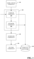
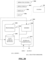
- the system 100 can predict cardinality of subgraphs of the query using one or more stored cardinality models, as discussed below.
- the system 100 includes a compiler component 110 that retrieves cardinality models relevant to the query from a model server component 130.
- the compiler component 110 can provide the cardinality models as annotation(s) to an optimizer component 120.
- the optimizer component 120 can extract and compute features for subgraphs of the query.
- the optimizer component 120 can retrieve cardinality models based upon the features of subgraphs of the query.
- the optimizer component 120 can further predict cardinality of the subgraphs using the retrieved cardinality models.
- the optimizer component 120 can select one of the subgraphs to utilize for the query based on the predicted cardinalities.
- a scheduler component 140 schedules execution of the query based upon the selected subgraph.
- a runtime component 150 executes the query based upon the selected subgraph.
- the compiler component 110 can provide compiled query directed acyclic graphs ("DAGs" also referred herein as "subgraphs") to a workload data store 160.
- DAGs compiled query directed acyclic graphs
- the optimizer component 120 can provide optimized plan(s) and/or estimated statistics regarding the selected subgraph to the workload data store 160.
- the scheduler component 140 can provide information regarding execution graph(s) and/or resource(s) regarding the selected subgraph to the workload data store 160.
- the runtime component 150 can provide actual runtime statistics regarding the selected subgraph to the workload data store 160.
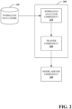
- the system 200 includes a workload analyzer component 210 that analyzes workload data (e.g., stored in the workload data store 160) to extract and compute features for training cardinality models stored in the model server component 130.
- workload data e.g., stored in the workload data store 160
- the extracted and computed features are discussed more fully below.
- the system 200 further includes a trainer component 220 that, using a machine learning algorithm, trains cardinality models stored in the model server component 130 based on the features of subgraphs of queries and actual runtime statistics included in the workload data (e.g., stored in the workload data store 160).
- the machine learning algorithms are discussed more fully below.
- the trainer component 220 stores the trained cardinality models in the model server component 130.
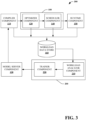
- Fig. 3 illustrates a feedback loop architecture 300 that includes the system for predicting cardinality of subgraphs of a query 100 and the system for training a cardinality model 200, as discussed below.
- Cardinality estimation is a difficult problem due to unknown operator selectivities (ratio of output and input data sizes) and correlations between different pieces of the data (e.g., columns, keys). Furthermore, the errors propagate exponentially thus having greater impact for queries with larger DAGs. The problem becomes even more difficult in the big data space due to the presence of large amounts of both structured as well as unstructured data and the pervasive use of custom code via user defined functions. Unstructured data has schema imposed at runtime (e.g., on the fly) and so it can be difficult to collect cardinality statistics over the data. Likewise, user code can embed arbitrary application logic resulting in arbitrary output cardinalities.
- the subject disclosure utilizes cardinality models trained from previous executions (e.g., via a feedback loop) thus benefiting from the observation that shared cloud workloads are often repetitive and overlapping in nature.
- the subject disclosure utilizes an active learning approach to explore and discover alternative query plan(s) in order to overcome learning bias in which alternate plans that have high estimated cardinalities but lower actual cardinalities are not tried resulting in a local optima trap.
- the machine learning based approach to improve cardinality estimates occurs at each point in a query graph.
- Subgraph templates that appear over multiple queries are extracted and a cardinality model is learned over varying parameters and inputs to those subgraph templates.
- SCOPE refers to a SQL-like language for scale-out data processing.
- a SCOPE data processing system processes multiple exabytes of data over hundreds of thousands of jobs running on hundreds of thousands of machines.
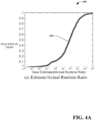
- Fig. 4(A) is a graph 400 that illustrates a cumulative distribution 410 of the ratio of estimated costs and the actual runtime (costs) of different subgraphs.
- the estimated costs are up to 100,000 times overestimated and up to 10,000 times underestimated than the actual ones.
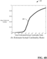
- Fig. 4(B) is a graph 420 that illustrates a cumulative distribution 430 of the ratio of estimated and actual cardinalities of different subgraphs.
- a small fraction of the subgraphs has estimated cardinalities matching the actual ones (i.e., the ratio is 1). Almost 15% of the subgraphs underestimate (by up to 10,000 times) and almost 85% of the subgraphs overestimate (by up to 1 million times).
- SCOPE workloads are also overlapping in nature: multiple jobs have common subgraphs across them. These jobs are further recurring in nature, for example, they are submitted periodically with different parameters and inputs.
- Fig. 4(C) is a graph 440 that illustrates a cumulative distribution 450 of subgraph overlap frequency. 40% of the subgraphs appear at least twice and 10% appear more than 10 times.
- subgraph overlaps can be leveraged to learn cardinalities in one job and reuse them in other jobs.
- the problem of improving cardinality estimates at different points in a query graph is considered.
- the requirements derived from the current production setting are as follows:
- a learning-based approach is applied to improve cardinalities using past observations. Subgraphs are considered and their output cardinalities are learned. Thus, instead of learning a single large model to predict possible subgraphs, a large number of smaller models (e.g., with few features) are learned, for example, one for each recurring template subgraph in the workload. In some embodiments, these large number of smaller models are highly accurate as well as much easier to understand. A smaller feature set also makes it easier to extract features during prediction, thereby adding minimal compilation overhead. Furthermore, since learning occurs over recurring templates, the models can be trained a priori (e.g., offline learning).
- the improved cardinalities are provided as annotation (e.g., hints) to the query that can later be applied wherever applicable by the optimizer. That is, the entire cardinality estimation mechanism is not entirely overwritten and the optimizer can still choose which hints to apply.
- annotation e.g., hints
- Modern query optimizers incorporate heuristic rule-based models to estimate the cardinalities for each candidate query plan.
- these heuristic models often produce inaccurate estimates, leading to significantly poor performance.
- predictive models can be learned and used to estimate the cardinalities (e.g., instead of using the heuristics).
- SCOPE SCOPE
- SCOPE SCOPE
- a goal is to be able to obtain accurate output row counts for every subgraph in each of the queries.
- the query subgraphs can be divided into five different categories depending on what part of the subgraph is considered fixed. Table 1 shows these categories and how they are different from each other: Table 1 Subgraph Type Operator Graph Parameters Data Inputs Most Strict ⁇ ⁇ ⁇ Recurring ⁇ ⁇ X Template ⁇ X ⁇ Recurring Template ⁇ X X Most General X X X
- Table 1 illustrates one extreme, the most strict subgraphs, where all three variables (operator graph, parameters, and data inputs) are fixed.
- the subgraph cardinalities observed in the past are recorded and reused in future occurrences of the exact same subgraphs. While these subgraphs are most accurate, such strict matches are likely to constitute a much smaller fraction of the total subgraphs in the workload (e.g., less than 10% on observed workloads). Hence low coverage is a challenge with the most strict subgraph matches.
- Table 1 illustrates the other extreme, where none of the operator graphs, the parameters, and data inputs are fixed.
- a single global model is learned that can predict cardinalities for all possible subgraphs, i.e., having full coverage.
- feature engineering e.g., featurizing subgraphs
- prediction latency e.g., gathering features during prediction
- getting features from the input data could require preprocessing that is simply not possible for ad-hoc queries.
- a middle ground can be taken in which cardinalities are learned for each recurring template subgraph (Table 1).
- a model is built for each operator subgraph, with varying parameters and inputs. This approach can have a number of advantages:
- One approach to learn cardinality is via collaborative filtering, which was traditionally developed for the matrix completion problem in recommender systems.
- a two-dimensional matrix M is built with the first dimension being an identifier of the query subgraph and the second dimension being an identifier of the input dataset.
- the entry M ij represents the output cardinality of applying query subgraph i to dataset j .
- the idea is as follows: given a small set of observed entries in this matrix, the missing (unobserved) entries are desired to be estimated. To do so, first matrix factorization is utilized to compute the latent factors of the query subgraphs and the datasets. Next, in order to predict the output cardinality of applying query subgraph i to dataset j , the latent factor of query subgraph i is multiplied with the latent factor of dataset j .
- the adjustment factor approach may suffer from three problems: (i) ignoring subgraphs and hence missing the changes in data distributions due to prior operations, (ii) presence of large amounts of user code which is often parameterized, and (iii) non-determinism.
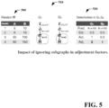
- diagrams 500, 510, 520 illustrate an impact of ignoring subgraphs in adjustment factors.
- R(A, B) of diagram 500 and two queries Q 1 and Q 2 of diagram 510 over the relation.
- Both Q 1 and Q 2 have 2 tuples as input to the filter predicate B ⁇ 100.
- both tuples qualify B ⁇ 100 in Q 1
- only one qualifies in Q 2 This is because columns A and B are correlated in R.
- a single adjustment factor does not work for predicate B ⁇ 100, since it is different for Q 1 and Q 2 . as shown in diagram 520.
- detecting such correlations is impractical in big data systems due to massive volumes of data, which is often unstructured and fast arriving. Adjustment factors are further nondeterministic, e.g., it could be 2 or 1 depending on whether Q 1 or Q 2 gets processed first.
- Table 2 shows the input and output cardinalities from multiple instances of a recurring reducer from the particular set of SCOPE workloads: Table 2 Input Cardinality Output Cardinality 672331 1596 672331 326461 672331 312 672331 2 672331 78 672331 1272 672331 45 672331 6482
- the reducer may receive the exact same input in all the instances; however, the output cardinalities can be very different. This is because the output cardinality depends on the parameters of the reducer. Hence, in some embodiments, simple adjustment factors will not work for complex queries with such user code. To validate this, the percentage error and Pearson correlation (between the actual and predicted cardinality) were compared for different approaches over this dataset. Table 3 shows the result: Table 3 Model Percentage Error Pearson Correlation Default Optimizer 2198654 0.41 Adjustment Factor 1477881 0.38 Linear Regression 11552 0.99 Neural Network 9275 0.96 Poisson Regression 696 0.98
- Table 3 shows that the adjustment factor improves slightly over the default optimizer estimates, but it still has a high estimation error and low correlation.
- feature-based machine learning models e.g., linear regression, Poisson regression and neural networks
- Table 4 Name Description JobName Name of the job containing the subgraph NormJobName Normalize job name InputCardinality Total cardinality of all inputs to the subgraph Pow (InputCardinality, 2) Square of InputCardinality Sqrt (InputCardinality) Square root of InputCardinality Log (InputCardinality) Log of InputCardinality AvgRowLength Average output row length InputDataset Name of all input datasets to the subgraph Parameters One or more parameters in the subgraph
- Metadata such as the name of the job the subgraph belongs to and the name of the input datasets was extracted.
- these metadata attributes are important as they could be used as inputs to user-defined operators.
- the reason that leads to the orders-of-magnitude difference in the output cardinality between the first and the second row in Table 2 is due to the difference in the name of the job the subgraph belongs to (e.g., everything else is the same for these two observations).
- the total input cardinality of all input datasets is extracted.
- the input cardinality plays a central role in predicting the output cardinality.
- the squared, squared root, and the logarithm of the input cardinality are computed as features.
- LR linear regression
- PR Poisson regression
- MLP multi-layer perceptron neural network
- LR linear regression
- PR Poisson regression
- MLP multi-layer perceptron
- LR is a purely linear model
- PR is slightly more complex and considered as a Generalized Linear Model (GLM).
- GLM Generalized Linear Model
- MLP provides for a fully non-linear, arbitrarily complex predictive function.
- the main advantage of using linear and GLM models is their interpretability.
- it is easy to extract the learned weights associated with each feature so that which features contribute more or less to the output cardinality can be more readily analyzed.
- This can be useful for many practical reasons as it gives the analysts an insight into how different input query plans produce different output cardinalities.
- This simplicity and explainability can however come at a cost: the linear model may not be sufficiently complex to capture the target cardinality function. In machine learning, this is known as the problem of underfitting which puts a cap on the accuracy of the final model regardless of how large the training data is.
- LR can produce negative predictions which are not allowed in the problem since cardinalities are always non-negative. To rectify this problem, the model output can be adjusted after-the-fact so that it will not produce negative values.
- PR on the other hand, does not suffer from this problem as by definition it has been built to model (non-negative) count-based data.
- MLP provides a much more sophisticated and richer modeling framework that in theory is capable of learning the target cardinality function regardless of its complexity, given that access to sufficient training data is provided.
- training and using an MLP for cardinality estimation can be more challenging than that of LR or PR for some fundamentally important reasons.
- using an MLP requires careful designing of the neural network architecture as well as a significant hyper-parameter tuning effort, which in turn requires a deep insight into the problem as well as the model complexity.
- the features that contribute to the models' prediction are analyzed as follows.
- the models produced by the Poisson regression algorithm are analyzed because Poisson regression offered the best performed in some embodiments, as discussed below.
- the features that do not contribute much to the prediction are given zero weight and are not included in the model. Therefore, by analyzing the set of features that appear in the model, which features contribute more to the prediction result can be learned. Fig.
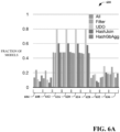
- 6(A) is a bar graph 600 that illustrates the fraction of the models that contain each of the features: JobName 604, NormJobName 608, InputCard 612, PowInputCard 616, SqrtInputCard 620, LogInputCard 624, AvgRowLength 628, InputDataset 632, and Params 636. Since each model can have a different number of parameters as features, these parameters are grouped into one feature category named 'Parameters' 636. In some embodiments, across all models trained, it can be observed that InputCardinality 612 plays a central role in model prediction as near 50% of the models contain InputCardinality 612 as a feature.
- the squared 616, squared root 620, and logarithm 624 of the input cardinality also can have a big impact on the prediction. In fact, their fractions are a bit higher than InputCardinality 612. Interestingly, all other features also provide a noticeable contribution. Even the least significant feature, AvgRowLength 628, appears in more than 10% of the models.
- the models can be further grouped based on the root operator of the subgraph template, and models whose root operators are Filter, user-defined object (UDO), Join, and Aggregation are analyzed.
- the graph 600 includes data for five groups of operators "All", “Filter” "UDO” (User-defined object), "HashJoin” and "HashBgAgg” from left to right.
- UDO User-defined data transformations for UDOs.
- Fig. 6(B) is a graph 640 that shows cumulative distributions "All" 644, "Filter” 648 , "UDO” 652, "HashJoin” 656, “HashGbAgg” 660 of the fraction of models that have a certain number of features with non-zero weight. Overall, it can be observed that more than 55% of the models have at least 3 features that contribute to the prediction, and 20% of the models have at least 6 features. It is worth noting that for models whose root operator are UDOs, more than 80% of the models have at least 5 features. This implies that, in some embodiments, a number of features are needed to jointly predict the output cardinality for subgraphs with complex operators like UDO.
- the feature-based framework cannot make predictions for unobserved subgraph templates. More data more data can be collected by observing more templates, during the training phase. However, the model still may be unable to improve the performance of ad hoc queries with new subgraph templates.
- the number of models grows linearly with respect to the number of distinct subgraph templates observed. Therefore, in the case of a limited storage budget, the models can be ranked and filtered based on effectiveness in fixing the wrong cardinality estimation produced by the query optimizer.
- the query optimizer chooses an execution path with the lowest cost.
- the cost of the first path is computed using the learning model's predicted cardinality and the cost of the second path is computed using the optimizer's default cardinality estimation (e.g., due to missing subgraph template models)
- directly comparing the two costs could lead to inaccuracy as the optimizer's default cardinality estimation could be heavily overestimating and/or underestimating the cardinality.
- FIG. 7 is a diagram 700 that illustrates an example of three alternate plans for joining relations X, Y, and Z , plan1 710, plan2 720 and plan3 730.
- plan1 710 For the first time, X Y (plan1 710) has lower estimated cost than X Z and Y Z, and so it will be picked.
- plan1 710 Once plan1 710 is executed, the actual cardinality of X Y is 100 is known, which is higher than the estimated cardinality of X Z. Therefore, the second time, the optimizer will pick plan2 720.
- Y Z is the least expensive option, it is never explored since the estimated cardinality of Y Z is higher than any of the actual cardinalities observed so far.
- a mechanism to explore alternate join orders and build cardinality models of those alternate subgraphs is desired, which can have higher estimated costs but may actually turn out to be less expensive.
- an exploratory join ordering technique is utilized to consider alternate join orders, based on prior observations, and ultimately discover the best one.
- the core idea is to leverage existing cardinality models and actual runtime costs of previously executed subgraphs to: (i) quickly explore alternate join orders and build cardinality models over the corresponding new subgraphs, and (ii) prune expensive join paths early so as to reduce the search space.
- having cardinality models over all possible alternate subgraphs naturally leads to finding the best join order eventually.
- the number of join orders are typically exponential and executing all of them one by one is simply not possible, even for a small set of relations. Therefore, a technique to quickly prune the search space to only execute the interesting join orders is desired.
- exploring join orders which involve that subgraph plan can be stopped. For instance, if A C is more expensive than ((A B) C) D, then join orders ((A C) B) D and ((A C) D) B can be pruned, i.e., all combinations involving A C are discarded as the total cost is going to be even higher anyways.
- the function returns null (Line 3) when the runtime cost of the subgraph plan is more expensive than the cost of the best query plan seen so far; otherwise, it returns the input plan with either the predicted cardinalities (Line 5) or the default estimated cardinalities (Line 6), depending on whether the subgraph has been seen before in previous executions or not.
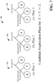
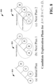
- Fig. 8 is a diagram 800 that illustrates an exploration comparator in which the planner first executes the plan shown in (a) 810 and then considers next plan 1 and next plan 2, shown in (b) 820 and (c) 830.
- the planner makes only one new observation with plan 1 (820), namely A B D, as A B and A B D C (which is equivalent to A B C D in terms of cardinality) have already been observed.
- next plan 2 (830) the planner makes two new observations, namely C D and C D A.
- next plan 2 (830) is better in terms of number of new observations than next plan 1.
- next plan 1 (820) and next plan 2 (830) would have had the same number of observations.
- the early pruning strategy and the exploration plan comparator can be integrated into a query planner for exploratory join ordering.
- Algorithm 3 pseudo code shows the exploratory version of System R style bottom-up planner, also sometimes referred to as Selinger planner:
- the planner starts with leaf level plans, i.e., scans over each relation, and incrementally builds plans for two, three, and more relations. For each candidate outer and inner plans, the algorithm checks to see if it can prune the search space (Lines 10-13). Otherwise, a comparison is made (using the exploration comparator) regarding the best plan to join outer and inner, with the previous best seen before (Lines 14-16). Only if a better plan is found, it is added to the current best plans (Line 17). Finally, the best plan for the overall query is returned (Line 18).
- other query planners can be extended, such as a top-down query planner or a randomized query planner, to explore alternate join orders and eventually find the best join order.
- a three-step template to convert a given query planner into an exploratory one is provided: (i) Enumerate: Iterate over candidate plans using the planner's enumeration strategy, e.g., bottom-up, top-down, (ii) Prune: Add pruning in the planner to discard subgraphs based on prior executions in the plan cache, i.e., subgraphs that were more expensive than the full query need not be explored anymore (e.g., this is in addition to any existing pruning in the planner), and (iii) Rank: Consider the number of new observations made when comparing and ranking equivalent plans. Additionally, costs can be incorporated by breaking ties using less expensive plans, or by considering observations only for plans with similar costs.
- one or more execution strategies can be employed with the system 100, the system 200, and/or the system 300, as discussed below.
- a natural strategy is to run multiple instances of subgraphs differently, i.e., apply the exploratory join ordering algorithm and get different plans for those instances. Furthermore, every instance of every subgraph run differently could be run until all alternative subgraphs have been explored, i.e., cardinality models for those alternate subgraphs have been learned and can pick the optimal join orders. Alternatively, since alternative subgraphs can be expensive, every other instance of every other subgraph run differently can be run to limit the number of outliers.
- queries can be tuned upfront by running multiple trials, each with different join ordering, over the same static data.
- proposed techniques can quickly prune down the search space, thereby making the number of trials feasible even for fairly complex jobs.
- sample runs can be used for resource optimization, i.e., for finding the best hardware resources for a given execution plan.
- Samples to learn cardinality models during static workload tuning can be used. For example, samples can be built using the traditional a priori sampling, or the more recent just-in-time sampling.
- the system 300 can be used to learn cardinality models and generate predictions during query processing.
- a first step in the feedback loop is to collect traces of past query runs from different components, namely the compiler component 110, the optimizer component 120, the scheduler component 140, and the runtime component 150.
- the SCOPE infrastructure is already instrumented to collect such traces. These traces are then fed to the workload analyzer component 210 which (i) reconciles the compile-time and runtime statistics, and (ii) extracts the training data, i.e., subgraph templates and their actual cardinalities.
- combining compile-time and run-time statistics requires mapping the logical operator tree to the data flow that is finally executed.
- the logical operator tree can be traversed in a bottom-up fashion and emit a subgraph for every operator node.
- the parameters are detected by parsing the scalar operators in the subgraph, and the leaf level inputs are detected by tracking the operator lineage.
- a unique hash is used, similar to plan signatures or fingerprints, that is recursively computed at each node in the operator tree to identify the subgraph template.
- the leaf level inputs and the parameter values are excluded from the computation as subgraphs that differ only in these attributes belong to the same subgraph template.
- the features discussed above are extracted and together with the subgraph template hash they are sent to the trainer component 220.
- the trainer component 220 can implement a parallel model trainer that can significantly speed up the training process.
- SCOPE can be used to partition the training data for each subgraph template, and build the cardinality model for each of them in parallel using a reducer. Within each reducer, a machine learning algorithm can be used to train the model.
- the machine learning algorithm can include a linear regression algorithm, a logistic regression algorithm, a decision tree algorithm, a support vector machine (SVM) algorithm, a Naive Bayes algorithm, a K-nearest neighbors (KNN) algorithm, a K-means algorithm, a random forest algorithm, a dimensionality reduction algorithm, and/or a Gradient Boost & Adaboost algorithm.
- the reducer in addition to the model, the reducer also emits the training error and the prediction error for the ten-fold cross validation.
- the reducer can also be configured to group these statistics by the type of the root operator of the subgraph template. This can help in an investigation of which type of subgraph template model is more effective compared to the optimizer's default estimation.
- the trained models are stored in the model server component 130.
- the model server component 130 is responsible for storing the models trained by the trainer component 220. In some embodiments, for each subgraph hash, the model server component 130 keeps track of the corresponding model along with its priority level and confidence level. In some embodiments, priority level is determined by how much improvement this model can achieve compared to the optimizer's default estimation. In some embodiments, confidence level is determined by the model's performance on a ten-fold cross validation. In some embodiments, the models with high priority levels can be cached into the database to improve the efficiency of model lookup. Note that in some embodiments, caching substantially all models into the database can be impractical due to limited storage resources.
- the model server component 130 can build an inverted index on the job metadata (which often remains the same across multiple instances of a recurring job) to return relevant cardinality models for a given job in a single call.
- the compiler component 110 and the optimizer 120 are responsible for model lookup and prediction.
- the compiler component 110 fetches relevant cardinality models for the current job and passes them as annotations to the optimizer component 120.
- each annotation contains the subgraph template hash, the model, and the confidence level.
- the optimizer component 120 prunes out the false positives by matching the subgraph template hash of the model with the hashes of each subgraph in the job graph. For matching subgraphs, the optimizer component 120 generates the features and applies them to the corresponding model to obtain the predicted cardinality.
- the compiler component 110 and/or the optimizer component 120 can prune models with sufficiently low confidence level.
- any row count hints from the user (in their job scripts) can still supersede the predicted cardinality values.
- predicted cardinalities can also persisted into the query logs for use during debugging, if needed.
- the cardinality models can be retrained for different reasons: (i) applying cardinality predictions results in new plans which means new subgraph templates, and hence the cardinality models need to be retrained until the plans stabilize, and (ii) the workloads can change over time and hence many of the models are not applicable anymore. Therefore, in some embodiments, periodic retraining of the cardinality models is performed to update existing models as well as adding new ones. In some embodiments, the timing of retraining can be performed based on the cardinality model coverage, i.e., the fraction of the subgraphs and jobs for which the models are available. Retraining can occur when those fractions fall below a predetermined threshold. In some embodiments, based upon experimental data, one month is a reasonable time to retrain the cardinality models.
- exploratory join ordering executes alternate subgraphs that can be potentially expensive.
- human(s) e.g., users, admins
- the exploratory join ordering algorithm can be run separately to produce a next join order given the subgraphs seen so far.
- User(s) can then enforce the suggested join order using the FORCE ORDER hint in their job scripts, which is later enforced by the SCOPE engine during optimization. Users can apply these hints to their recurring/overlapping jobs, static tuning jobs, or pilot runs over sample data.
- the training accuracy, cross-validation, and coverage of the learned cardinality models of the exemplary feedback loop architecture 300 are first evaluated.
- Figs. 9(A)-9(C) illustrate cardinality model training results of the exemplary feedback loop architecture.
- Fig. 9(A) is a graph 900 illustrating a comparison of percentage error vs. fraction of subgraph templates for a default optimizer 904, a multi-layer perceptron neural network 908, a fast linear regression 912 and Poisson regression 916.
- Fig. 9(A) shows the results over 34,065 subgraph templates.
- the prediction error from the optimizer's default estimation is included as a baseline comparison 904.
- the training error of all three models is less than 10%.
- the baseline 904 only 15% of the subgraph templates achieve the same level of performance. Therefore, the learning models significantly outperform the baseline.
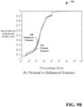
- Fig. 9(B) is a graph 920 illustrating the effect of using the enhanced features on the prediction accuracy.
- the graph 920 includes a distribution of normal features 924 and a distribution of enhanced features 928.
- the enhanced features 928 include the square, square root, and log of input cardinality discussed above in order to account for operators that can lead to a non-linear relationship between the input and output cardinality. It is observed that adding these features does lead to a slight performance improvement in terms of the training accuracy. More importantly, as discussed below, the enhanced features can lead to new query plan generations when feeding back cardinalities produced by our model.
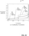
- Fig. 9(C) is a graph 932 illustrating the Pearson correlation between the predicted cardinality and the actual cardinality for different models.
- the graph 932 includes a default optimizer distribution 936, a multi-layer perceptron neural network distribution 940, a fast linear regression distribution 944 and a Poisson regression distribution 948. It can be observed that fast linear regression and Poisson regression manage to achieve higher correlation than the baseline default optimizer. Surprisingly, although a neural network attains a very low training error, the correlation between its predicted cardinality and the actual cardinality is lower than the baseline.
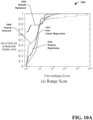
- Figs. 10(A) - 10(C) illustrate the training error of the exemplary models and the baseline on subgraph templates whose root operators are range scan, filter, and hash join.
- Fig. 10(A) is a graph 1000 that includes a default optimizer distribution 1004, a multi-layer perceptron neural network distribution 1008, a fast linear regression distribution 1012 and a Poisson regression distribution 1016.
- Fig. 10(B) is a graph 1020 that includes a default optimizer distribution 1024, a multi-layer perceptron neural network distribution 1028, a fast linear regression distribution 1032 and a Poisson regression distribution 1036.
- Fig. 10(C) is a graph 1040 that includes a default optimizer distribution 1044, a multi-layer perceptron neural network distribution 1048, a fast linear regression distribution 1052 and a Poisson regression distribution 1056.
- the default optimizer's estimation 1004 (baseline performance) is in fact comparable to the exemplary models 1008, 1012, 1016.
- the exemplary models 1008, 1012, 1016 perform significantly better than the baseline 1004.
- some models are more important than others as they can provide far more accurate cardinality estimation than using the baseline. Therefore, in some embodiments, this information can assist in the decision of which model to materialize when a limited storage budget is involved.
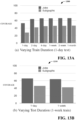
- Fig. 11(A) is a validation graph 1100 that includes an actual distribution 1104, a multi-layer perceptron neural network distribution 1108, a fast linear regression distribution 1112 and a Poisson regression distribution 1116.
- Fig. 11(A) illustrates the cumulative distributions of predicted and actual cardinalities. It can be observed that both fast linear 1112 and Poisson regression 1116 follow the actual cardinality distribution 1104 very closely.
- Fig. 11(B) is a validation graph 1120 that includes a multi-layer perceptron neural network distribution 1124, a fast linear regression distribution 1128 and a Poisson regression distribution 1132.
- Fig. 11(B) illustrates the percentage error of different prediction models 1124, 1128, 1132.
- Poisson regression 1132 has the lowest error, with 75th percentile error of 1.5% and 90th percentile error of 32%. This is compared to 75th and 90th percentile errors of 74602% and 5931418% respectively for the default SCOPE optimizer.
- the neural network 1124 achieves the smallest training error, it exhibits the largest prediction error when it comes to cross-validation. This is likely due to overfitting given the large capacity of the neural network and the relatively small observation space and feature space, as also discussed above.
- Fig. 11(C) is a graph 1136 that includes a multi-layer perceptron neural network distribution 1140, a fast linear regression distribution 1144 and a Poisson regression distribution 1148.
- Fig. 11(C) illustrates the ratio between the model's 1140, 1144, 1148 predicted cardinality and the actual cardinality for each subgraph. It can be observed that the ratio is very close to 1 for most of the subgraphs across all three models 1140, 1144, 1148.
- fast linear regression 1144 and Poisson regression 1148 it can be observed that neural network 1140 overestimates 10% of the subgraphs by over 10 times. This may be due to the aforementioned overfitting. Nevertheless, compared to the Fig. 4(B) generated using the optimizer's estimation, all of the models 1140, 1144, 1148 achieve significant improvement.
- the subgraph coverage can be defined as the percentage of subgraphs having a learned model and the job coverage as percentage of jobs having a learned cardinality model for at least one subgraph.
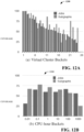
- Fig. 12(A) is a bar chart 1200 illustrating the coverage for different virtual clusters (VCs) - 58 (77%) VCs have at least 50% jobs (subgraphs) impacted. The jobs/subgraphs are further subdivided into CPU-hour and latency buckets and the coverage evaluated over different buckets.
- Figures 12(B) and 12(C) are bar charts 1210, 1220 illustrating the results. Interestingly, the fraction of subgraphs impacted decreases both with larger CPU-hour and latency buckets. In some embodiments, this is because there are a fewer number of jobs in these buckets and hence less overlapping subgraphs across jobs. Still more than 50% of the jobs are covered in the largest CPU-hour bucket and almost 40% are covered in the largest latency bucket.
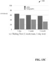
- Fig. 13(A) is a bar chart 1300 that illustrates the coverage over varying training durations from one day to one month and testing one day after. It can be observed that two-day training already brings the coverage close to the peak (45% subgraphs and 65% jobs). In some embodiments, this is because most of the workload comprises daily jobs and a two-day window captures jobs that were still executing over the day boundary. This is further reflected in the bar chart 1310 of Fig. 13(B) , where the coverage remains unchanged when the test window is varied from a day to a week. Finally, the one-day testing window is slid by a week and by a month in the bar chart 1320 of Fig. 13(C) . In some embodiments, it can be observed that the coverage drop is noticeable when testing after a month, indicating that this is a good time to retrain in order to adapt to changes in the workload.
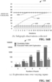
- the bar chart 1400 includes an enhanced multi-layer perceptron neural network bar 1404, an enhanced Poisson regression bar 1408, an enhanced fast linear regression bar 1412, a multi-layer perceptron neural network bar 1416, a Poisson regression bar 1420 and a fast linear regression bar 1424.
- the bar chart 1400 of Fig. 14(A) shows that when training models using standard features, on an average, only 11% of the jobs experience changes in query plans. However, once the enhanced features are incorporated into the models, these percentages go up to 28%. This is because the enhanced features capture the non-linear relationships between the input and output cardinality and are significant to the model performance. Overall, it can be observed that applying the models yield significant changes to the optimizer's generated query plans.
- Fig. 14(B) is a graph 1428 that includes a multi-layer perceptron neural network distribution 1432, a fast linear regression distribution 1436 and a Poisson regression distribution 1440.
- Fig. 14(B) illustrates the absolute change for all three models 1432, 1436, 1440. It can be observed that a 75th percentile cost change of 79% and 90th percentile cost change of 305%. Thus, the high accuracy cardinality predictions from the models ( Fig. 11(C) do indeed impact and rectify the estimated costs significantly.
- Fig. 14(C) is a graph 1444 that includes a distribution 1448 illustrating the percentage new subgraphs generated in the recompiled jobs due to improved cardinalities.
- a distribution 1448 illustrating the percentage new subgraphs generated in the recompiled jobs due to improved cardinalities.
- the performance improvement when using the feedback loop of learned models is next evaluated.
- three items can be considered for the evaluation: (i) the end-to-end latency which indicates the performance visible to the user, (ii) the CPU-hours which indicates the cost of running the queries in a job service, and (iii) the number of containers (or vertices) launched which indicates the resource consumption.
- Eight different production recurring jobs were selected, each of which get executed multiple times in a day and having default end-to-end latency within 10 minutes. These jobs were executed with and without feedback by directing the output to a particular location.
- the opportunistic scheduling was disabled to make the measurements from different queries comparable.
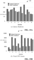
- Fig. 15(A) is a bar chart 1500 that illustrates the end-to-end latencies of each of the queries with and without the feedback loop. It can be observed that the latency improvement is variable and sometimes it is simply not there (queries 2, 4, and 8). This is because latency improvements depend on whether or not the changes in the plan are on the critical path. Still, a 25% improvement in total latency can be observed, which is valuable for improving user experience on SCOPE.
- Fig. 15(B) is a bar chart 1510 that compares the CPU-hours of queries with and without the feedback loop. The improvements are much more significant here because even though the plan change may not be on the critical path of the query, it still translates to fewer CPU-hours. Overall, there is a 55% drop in total CPU-hours, which is significant for dollar savings in terms of operational costs.
- Fig. 15(C) is a bar chart 1520 that illustrates the total number of vertices (containers) launched by each of the queries.
- the savings are much more significant. This is consistent with the discussion above regarding how the default optimizer significantly overestimates the cardinalities most of the times, resulting in a large number of containers to be launched, each with a very small amount of data to process. Tighter cardinality estimations, using the exemplary models, help avoid wasting these resources. Overall, 60% less vertices were launched using the feedback loop.
- the effectiveness of the exploratory bottom-up query planning algorithm is next evaluated.
- the focus of the evaluation is to show how quickly the algorithm prunes the search space, exploits unobserved subgraph, and finds the optimal plan.
- a prototype provides the join ordering hints which the users can later enforce in their scripts.
- the synthetic workload contains a join query over 6 randomly generated tables with varying cardinalities, where any pair of tables can have a join predicate with probability 0.8, and a random join selectivity between 0 to 1.
- Fig. 16(A) is a graph 1600 that includes an optimizer without feedback distribution 1604, an optimizer with feedback distribution 1608, an optimizer with exploratory join ordering distribution 1612 and an optimum distribution 1616.
- Fig. 16(A) compares the cost of the plans chosen by the exploratory algorithm against the plans chosen by several alternatives.
- the planner is able to explore all unobserved subgraphs in 17 more iterations, and eventually find the optimal plan.
- the exploratory algorithm considers more expensive alternative(s), however, it prunes out the really expensive ones and never considers the plans more expensive than those produced by the naive Selinger planner.
- Fig. 16(B) is a graph 1620 including an optimizer without feedback distribution 1624, an optimizer with feedback distribution 1628, an optimizer with exploratory join ordering 1632, and, a total distribution 1634.
- Fig. 16(B) illustrates that while the naive Selinger planner and the planner with feedback can only explore a small subset of the subgraphs and build cardinality models over them, the exploratory planner is able to quickly cover all subgraphs in 17 more iterations. The cardinality models built over those newly observed subgraphs could be useful across multiple other queries, in addition to helping find the optimal plan for the current query.
- Fig. 16(C) is a bar chart 1640 illustrating the number of redundant executions needed for complete exploration when varying the number of inputs. It can be observed that while the candidate paths grow exponentially, the number of executions required for the exploratory planner to find the optimal plan only grows in polynomial fashion, e.g., just 31 runs for 7 join inputs. The reason is that the exploratory planner picks the plan that maximizes the number of newly subgraph observations, and the number of distinct subgraphs grows in a polynomial manner with the number of inputs. Once the planner has built cardinality feedback for most subgraphs, it can produce the optimal plan.
- the above evaluation was repeated on the TPC-H dataset (i.e., from http:///www.tpc.org/tpch) using a query that de-normalizes all tables.
- the exploration planner was able to explore and build all relevant cardinality models using just 36 out of the 759 possible runs.
- the exploratory join ordering planner is indeed able to quickly prune the search space and explore alternative subgraphs, thereby avoiding the bias in learning cardinalities and producing optimal plans eventually.
- Figs. 17-19 illustrate exemplary methodologies relating to training cardinality models and/or using trained cardinality models to predict cardinality. While the methodologies are shown and described as being a series of acts that are performed in a sequence, it is to be understood and appreciated that the methodologies are not limited by the order of the sequence. For example, some acts can occur in a different order than what is described herein. In addition, an act can occur concurrently with another act. Further, in some instances, not all acts may be required to implement a methodology described herein.
- the acts described herein may be computer-executable instructions that can be implemented by one or more processors and/or stored on a computer-readable medium or media.
- the computer-executable instructions can include a routine, a sub-routine, programs, a thread of execution, and/or the like.
- results of acts of the methodologies can be stored in a computer-readable medium, displayed on a display device, and/or the like.
- a method of training cardinality models 1700 is illustrated. In some embodiments, the method 1700 is performed by the system 200.
- a workload data is analyzed to extract and compute features for subgraphs of queries.
- cardinality models e.g., one for each subgraph
- the trained cardinality models are stored.
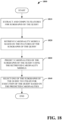
- a method of predicting cardinality of subgraphs of a query is illustrated.
- the method 1800 is performed by the system 100.
- features for subgraphs of the query are extracted and computed.
- cardinality models are retrieved based on the features of subgraphs of the query (e.g., matching subgraphs).
- cardinalities of the subgraphs of the query are predicted using the retrieved cardinality models.
- one of the subgraphs of the query is selected to be utilized for execution of the query based on the predicted cardinalities.
- a method of predicting cardinality of subgraphs of a query is illustrated.
- the method 1900 is performed by the system 300.
- workload data is analyzed to extract and compute features of subgraphs of queries.
- cardinality models are trained using a machine learning algorithm based on the features and actual runtime statistics include in the workload data.
- the trained cardinality models are stored.
- features for subgraphs of the query are extracted and computed.
- cardinality models are retrieved based on the features of the subgraphs of the query.
- cardinalities of the subgraphs of the query are predicted using the cardinality models.
- one of the subgraphs is selected to be utilized for execution of the query based on the predicted cardinalities.
- a system for training cardinality models comprising: a computer comprising a processor and a memory having computer-executable instructions stored thereupon which, when executed by the processor, cause the computer to: analyze workload data to extract and compute features of subgraphs of queries; using a machine learning algorithm, train the cardinality models based on the features and actual runtime statistics included in the workload data; and store the trained cardinality models.
- the system can include wherein the extracted features comprise, for a particular subgraph of a particular query, at least one of a job name, a total cardinality of all inputs to the particular subgraph, a name of all input datasets to the particular subgraph, or one or more parameters in the particular subgraph.
- the system can further include wherein the computed features comprise, for a particular subgraph of a particular query, at least one of a normalized job name, a square of an input cardinality of the particular subgraph, a square root of the input cardinality of the particular subgraph, a log of the input cardinality of the particular subgraph, or an average output row length.
- the system can include wherein the cardinality models are based on at least one of a linear regression algorithm, a Poisson regression algorithm, or a multi-layer perceptron neural network.
- the system can further include wherein at least one of a priority level or a confidence level is stored with the trained cardinality models.
- the system can include the memory having computer-executable instructions stored thereupon which, when executed by the processor, cause the computer to: during training of the cardinality models, whenever a particular subgraph is more computationally expensive than a full query plan, stop exploring join orders which involve that particular subgraph.
- the system can include the memory having further computer-executable instructions stored thereupon which, when executed by the processor, cause the computer to: during training of the cardinality models, for two equivalent subgraphs, select a particular subgraph which maximizes a number of new subgraphs observed.
- the system can include the memory having further computer-executable instructions stored thereupon which, when executed by the processor, cause the computer to: extract and compute features for subgraphs of a query; retrieve cardinality models based on the features of the subgraphs of the query; predict cardinalities of the subgraphs of the query using the retrieved cardinality models; and select one of the subgraphs of the query to utilize for execution of the query based on the predicted cardinalities.
- Described herein is a method of predicting cardinality of subgraphs of a query, comprising: extracting and computing features for the subgraphs of the query; retrieving cardinality models based on the features of the subgraphs of the query; predicting cardinalities of the subgraphs of the query using the retrieved cardinality models; and selecting one of the subgraphs of the query to utilize for execution of the query based on the predicted cardinalities.
- the method can include executing the query using the selected subgraph of the query.
- the method can further include wherein the extracted features comprise, for a particular subgraph of a particular query, at least one of a job name, a total cardinality of all inputs to the particular subgraph, a name of all input datasets to the particular subgraph, or one or more parameters in the particular subgraph.
- the method can include wherein the computed features comprise, for a particular subgraph of a particular query, at least one of a normalized job name, a square of an input cardinality of the particular subgraph, a square root of the input cardinality of the particular subgraph, a log of the input cardinality of the particular subgraph, or an average output row length.
- the method can further include wherein the cardinality models are based on at least one of a linear regression algorithm, a Poisson regression algorithm, or a multi-layer perceptron neural network.
- the method can further include wherein at least one of a priority level or a confidence level is stored with the trained cardinality models and used when selecting one of the subgraphs of the query to utilize for execution of the query.
- Described herein is a computer storage media storing computer-readable instructions that when executed cause a computing device to: analyze workload data to extract and compute features of subgraphs of queries; using a machine learning algorithm, train the cardinality models based on the features and actual runtime statistics included in the workload data, and store the trained cardinality model; extract and compute features for the subgraphs of the query; retrieve cardinality models based on the features of the subgraphs of the query; predict cardinalities of the subgraphs of the query using the retrieved cardinality models; and select one of the subgraphs of the query to utilize for execution of the query based on the predicted cardinalities.
- the computer storage media can store further computer-readable instructions that when executed cause the computing device to: execute the query using the selected subgraph of the query.
- the computer storage media can further include wherein the extracted features comprise, for a particular subgraph of a particular query, at least one of a job name, a total cardinality of all inputs to the particular subgraph, a name of all input datasets to the particular subgraph, or one or more parameters in the particular subgraph.
- the computer storage media can further include wherein the computed features comprise, for a particular subgraph of a particular query, at least one of a normalized job name, a square of an input cardinality of the particular subgraph, a square root of the input cardinality of the particular subgraph, a log of the input cardinality of the particular subgraph, or an average output row length.
- the computer storage media can further include wherein the cardinality models are based on at least one of a linear regression algorithm, a Poisson regression algorithm, or a multi-layer perceptron neural network.
- the computer storage media can further include wherein at least one of a priority level or a confidence level is stored with the trained cardinality models and used when selecting one of the subgraphs of the query to utilize for execution of the query.
- an example general-purpose computer or computing device 2002 e.g., mobile phone, desktop, laptop, tablet, watch, server, hand-held, programmable consumer or industrial electronics, set-top box, game system, compute node.
- the computing device 2002 may be used in the system for predicting cardinality of subgraphs of a query 100, the system for training a cardinality model 200, and/or the feedback loop architecture 300.
- the computer 2002 includes one or more processor(s) 2020, memory 2030, system bus 2040, mass storage device(s) 2050, and one or more interface components 2070.
- the system bus 2040 communicatively couples at least the above system constituents.
- the computer 2002 can include one or more processors 2020 coupled to memory 2030 that execute various computer executable actions, instructions, and or components stored in memory 2030.
- the instructions may be, for instance, instructions for implementing functionality described as being carried out by one or more components discussed above or instructions for implementing one or more of the methods described above.
- the processor(s) 2020 can be implemented with a general purpose processor, a digital signal processor (DSP), an application specific integrated circuit (ASIC), a field programmable gate array (FPGA) or other programmable logic device, discrete gate or transistor logic, discrete hardware components, or any combination thereof designed to perform the functions described herein.
- a general-purpose processor may be a microprocessor, but in the alternative, the processor may be any processor, controller, microcontroller, or state machine.
- the processor(s) 2020 may also be implemented as a combination of computing devices, for example a combination of a DSP and a microprocessor, a plurality of microprocessors, multi-core processors, one or more microprocessors in conjunction with a DSP core, or any other such configuration.
- the processor(s) 2020 can be a graphics processor.
- the computer 2002 can include or otherwise interact with a variety of computer-readable media to facilitate control of the computer 2002 to implement one or more aspects of the claimed subject matter.
- the computer-readable media can be any available media that can be accessed by the computer 2002 and includes volatile and nonvolatile media, and removable and non-removable media.
- Computer-readable media can comprise two distinct and mutually exclusive types, namely computer storage media and communication media.
- Computer storage media includes volatile and nonvolatile, removable and non-removable media implemented in any method or technology for storage of information such as computer-readable instructions, data structures, program modules, or other data.
- Computer storage media includes storage devices such as memory devices (e.g., random access memory (RAM), read-only memory (ROM), electrically erasable programmable read-only memory (EEPROM)), magnetic storage devices (e.g., hard disk, floppy disk, cassettes, tape), optical disks (e.g., compact disk (CD), digital versatile disk (DVD)), and solid state devices (e.g., solid state drive (SSD), flash memory drive (e.g., card, stick, key drive)), or any other like mediums that store, as opposed to transmit or communicate, the desired information accessible by the computer 2002. Accordingly, computer storage media excludes modulated data signals as well as that described with respect to communication media.
- RAM random access memory
- ROM read-only memory
- EEPROM electrically erasable programmable read-only memory
- Communication media embodies computer-readable instructions, data structures, program modules, or other data in a modulated data signal such as a carrier wave or other transport mechanism and includes any information delivery media.
- modulated data signal means a signal that has one or more of its characteristics set or changed in such a manner as to encode information in the signal.
- communication media includes wired media such as a wired network or direct-wired connection, and wireless media such as acoustic, RF, infrared and other wireless media.
- Memory 2030 and mass storage device(s) 2050 are examples of computer-readable storage media.
- memory 2030 may be volatile (e.g., RAM), non-volatile (e.g., ROM, flash memory) or some combination of the two.
- the basic input/output system (BIOS) including basic routines to transfer information between elements within the computer 2002, such as during start-up, can be stored in nonvolatile memory, while volatile memory can act as external cache memory to facilitate processing by the processor(s) 2020, among other things.
- BIOS basic input/output system
- Mass storage device(s) 2050 includes removable/non-removable, volatile/non-volatile computer storage media for storage of large amounts of data relative to the memory 2030.
- mass storage device(s) 2050 includes, but is not limited to, one or more devices such as a magnetic or optical disk drive, floppy disk drive, flash memory, solid-state drive, or memory stick.
- Memory 2030 and mass storage device(s) 2050 can include, or have stored therein, operating system 2060, one or more applications 2062, one or more program modules 2064, and data 2066.
- the operating system 2060 acts to control and allocate resources of the computer 2002.
- Applications 2062 include one or both of system and application software and can exploit management of resources by the operating system 2060 through program modules 2064 and data 2066 stored in memory 2030 and/or mass storage device (s) 2050 to perform one or more actions. Accordingly, applications 2062 can turn a general-purpose computer 2002 into a specialized machine in accordance with the logic provided thereby.
- system 100 or portions thereof can be, or form part, of an application 2062, and include one or more modules 2064 and data 2066 stored in memory and/or mass storage device(s) 2050 whose functionality can be realized when executed by one or more processor(s) 2020.
- the processor(s) 2020 can correspond to a system on a chip (SOC) or like architecture including, or in other words integrating, both hardware and software on a single integrated circuit substrate.
- the processor(s) 2020 can include one or more processors as well as memory at least similar to processor(s) 2020 and memory 2030, among other things.
- Conventional processors include a minimal amount of hardware and software and rely extensively on external hardware and software.
- an SOC implementation of processor is more powerful, as it embeds hardware and software therein that enable particular functionality with minimal or no reliance on external hardware and software.
- the system 100 and/or associated functionality can be embedded within hardware in a SOC architecture.
- the computer 2002 also includes one or more interface components 2070 that are communicatively coupled to the system bus 2040 and facilitate interaction with the computer 2002.
- the interface component 2070 can be a port (e.g., serial, parallel, PCMCIA, USB, FireWire) or an interface card (e.g., sound, video) or the like.
- the interface component 2070 can be embodied as a user input/output interface to enable a user to enter commands and information into the computer 2002, for instance by way of one or more gestures or voice input, through one or more input devices (e.g., pointing device such as a mouse, trackball, stylus, touch pad, keyboard, microphone, joystick, game pad, satellite dish, scanner, camera, other computer).
- pointing device such as a mouse, trackball, stylus, touch pad, keyboard, microphone, joystick, game pad, satellite dish, scanner, camera, other computer.
- the interface component 2070 can be embodied as an output peripheral interface to supply output to displays (e.g., LCD, LED, plasma), speakers, printers, and/or other computers, among other things. Still further yet, the interface component 2070 can be embodied as a network interface to enable communication with other computing devices (not shown), such as over a wired or wireless communications link.
- displays e.g., LCD, LED, plasma
- speakers e.g., speakers, printers, and/or other computers
- the interface component 2070 can be embodied as a network interface to enable communication with other computing devices (not shown), such as over a wired or wireless communications link.
Landscapes
- Engineering & Computer Science (AREA)
- Theoretical Computer Science (AREA)
- Physics & Mathematics (AREA)
- General Physics & Mathematics (AREA)
- Computational Linguistics (AREA)
- Data Mining & Analysis (AREA)
- General Engineering & Computer Science (AREA)
- Evolutionary Computation (AREA)
- Mathematical Physics (AREA)
- Artificial Intelligence (AREA)
- Software Systems (AREA)
- Computing Systems (AREA)
- Health & Medical Sciences (AREA)
- Life Sciences & Earth Sciences (AREA)
- Biomedical Technology (AREA)
- Biophysics (AREA)
- General Health & Medical Sciences (AREA)
- Molecular Biology (AREA)
- Databases & Information Systems (AREA)
- Operations Research (AREA)
- Information Retrieval, Db Structures And Fs Structures Therefor (AREA)
- Management, Administration, Business Operations System, And Electronic Commerce (AREA)
Claims (14)
- System, umfassend:mindestens einen Prozessor (2020); undeinen Speicher (2030) mit darauf gespeicherten, computerausführbaren Anweisungen, die, wenn sie von dem mindestens einen Prozessor ausgeführt werden, das System zu Folgendem veranlassen:Analysieren (1710, 1910) wiederkehrender Abfrage-Teilgraphen, um Merkmale von Operator-Teilgraphen von Abfragen zu bestimmen;unter Verwendung eines maschinellen Lernalgorithmus, Trainieren (1720, 1920) eines bestimmten Kardinalitätsmodells, um Kardinalitäten als Ausgabe vorherzusagen, für jeden bestimmten Operator-Teilgraphen der Operator-Teilgraphen, basierend auf mindestens den Merkmalen und tatsächlichen Laufzeitstatistiken, die in den wiederkehrenden Abfrage-Teilgraphen für mindestens zwei verschiedene Abfragen enthalten sind, die unterschiedliche Parameter oder unterschiedliche Dateneingaben einschließen, wobei der bestimmte Operator-Teilgraph eine Sequenz von Operatoren umfasst, die in den mindestens zwei verschiedenen Abfragen vorkommen;Speichern (1730) der bestimmten Kardinalitätsmodelle;Empfangen einer Abfrage, die bestimmte Operator-Teilgraphen aufweist, die verwendet werden können, um die Abfrage auszuführen;Abrufen (1950) jeweiliger Kardinalitätsmodelle für die bestimmten Operator-Teilgraphen;Vorhersagen (1960) von Kardinalitäten der bestimmten Operator-Teilgraphen unter Verwendung der jeweiligen Kardinalitätsmodelle; undAuswählen (1970) eines bestimmten Operator-Teilgraphen der bestimmten Operator-Teilgraphen, der die niedrigste Kardinalität aufweist, um ihn für die Ausführung der Abfrage zu verwenden.
- System nach Anspruch 1, wobei die Merkmale für ein Auftreten eines einzelnen Operator-Teilgraphen in einer einzelnen Abfrage in den Daten zur Arbeitslast mindestens eines von einem Abfragenamen des einzelnen Auftrags, einer Gesamtkardinalität aller Eingaben in den einzelnen Operator-Teilgraphen, einem Namen aller Eingabedatensätze in den einzelnen Operator-Teilgraphen oder einem oder mehreren Parametern in dem einzelnen Operator-Teilgraphen umfassen.
- System nach Anspruch 1, wobei die Merkmale für ein Auftreten eines einzelnen Operator-Teilgraphen in einer einzelnen Abfrage in den Daten der Arbeitslast mindestens eines von einem normalisierten Abfragenamen des einzelnen Auftrags, einem Quadrat einer Eingabekardinalität des einzelnen Operator-Teilgraphen, einer Quadratwurzel der Eingabekardinalität des einzelnen Operator-Teilgraphen, einem Logarithmus der Eingabekardinalität des einzelnen Operator-Teilgraphen oder einer durchschnittlichen Ausgangszeilenlänge umfassen.
- System nach Anspruch 1, wobei das bestimmte Kardinalitätsmodell basierend auf mindestens einem linearen Regressionsalgorithmus, einem Poisson-Regressionsalgorithmus oder einem mehrschichtigen neuronalen Perzeptron-Netzwerk ist.
- System nach Anspruch 1, wobei der Speicher weitere computerausführbare Anweisungen aufweist, die, wenn sie von dem Prozessor ausgeführt werden, das System zu Folgendem veranlassen:
während des Trainierens eines weiteren Kardinalitätsmodells für einen weiteren Operator-Teilgraphen, Bestimmen, dass der weitere Operator-Teilgraph rechenintensiver ist als ein vollständiger Plan für Abfragen, und Beenden der Untersuchung von Join-Anordnungen, die diesen einzelnen Operator-Teilgraphen beinhalten. - System nach Anspruch 1, wobei der Speicher weitere computerausführbare Anweisungen aufweist, die, wenn sie von dem Prozessor ausgeführt werden, das System zu Folgendem veranlassen:
während des Trainierens von Kardinalitätsmodellen für zwei äquivalente Operator-Teilgraphen, einschließlich des bestimmten Operator-Teilgraphen und eines weiteren Operator-Teilgraphen, Auswählen des bestimmten Operator-Teilgraphen für das Training, basierend auf mindestens einem Bestimmen, dass der bestimmte Operator-Teilgraph eine Anzahl von neuen Teilgraphen maximiert, die relativ zu dem weiteren Operator-Teilgraphen betrachtet werden. - Computerimplementiertes Verfahren, umfassend:Analysieren (1710, 1910) wiederkehrender Abfrage-Teilgraphen, um Merkmale einer Vielzahl von Operator-Teilgraphen zu bestimmen, wobei jeder Operator-Teilgraph eine Sequenz von zwei oder mehr Operatoren umfasst;unter Verwendung eines maschinellen Lernalgorithmus, Trainieren (1720, 1920) von Kardinalitätsmodellen, um Kardinalitäten als Ausgabe vorherzusagen, für jeden bestimmten Operator-Teilgraphen der Operator-Teilgraphen, basierend auf mindestens den Merkmalen und tatsächlichen Laufzeitstatistiken, die in den wiederkehrenden Abfrage-Teilgraphen für mindestens zwei verschiedene Abfragen enthalten sind, die unterschiedliche Parameter oder unterschiedliche Dateneingaben einschließen, wobei der bestimmte Operator-Teilgraph eine Sequenz von Operatoren umfasst, die in den mindestens zwei verschiedenen Abfragen vorkommen;Speichern (1730) der bestimmten Kardinalitätsmodelle;Empfangen einer Abfrage, die bestimmte Operator-Teilgraphen aufweist, die verwendet werden können, um die Abfrage auszuführen;Abrufen (1950) jeweiliger Kardinalitätsmodelle für die bestimmten Operator-Teilgraphen;Vorhersagen (1960) von Kardinalitäten der bestimmten Operator-Teilgraphen unter Verwendung der jeweiligen Kardinalitätsmodelle; undAuswählen (1970) eines bestimmten Operator-Teilgraphen der bestimmten Operator-Teilgraphen, der die niedrigste Kardinalität aufweist, um ihn für die Ausführung der Abfrage zu verwenden.
- Computerimplementiertes Verfahren nach Anspruch 7, ferner umfassend:
Ausführen der Abfrage unter Verwendung des bestimmten Operator-Teilgraphen. - Computerimplementiertes Verfahren nach Anspruch 7, wobei die Merkmale mindestens eines der folgenden Merkmale widerspiegeln: Abfragenamen, Eingabekardinalität, Eingabedatensatznamen oder Operator-Teilgraphenparameter.
- Computerimplementiertes Verfahren nach Anspruch 7, wobei die Merkmale mindestens eines der folgenden Merkmale widerspiegeln: normalisierte Abfragenamen, Quadrate von Eingabekardinalitäten, Quadratwurzeln von Eingabekardinalitäten, Logarithmen von Eingabekardinalitäten oder durchschnittliche Zeilenlängenausgaben.
- Computerimplementiertes Verfahren nach Anspruch 7, wobei die Kardinalitätsmodelle basierend auf mindestens einem linearen Regressionsalgorithmus, einem Poisson-Regressionsalgorithmus oder einem mehrschichtigen neuronalen Perzeptron-Netzwerk erstellt werden.
- Computerimplementiertes Verfahren nach Anspruch 7, wobei mindestens eine Prioritätsstufe oder eine Konfidenzstufe mit den Kardinalitätsmodellen gespeichert und bei der Auswahl des bestimmten Operator-Teilgraphen verwendet wird, der für die Ausführung der Abfrage verwendet werden soll.
- Computer-Speichermedium, das computerlesbare Anweisungen speichert, die bei Ausführung eine Rechenvorrichtung zu Folgendem veranlassen:Analysieren (1710, 1910) wiederkehrender Abfrage-Teilgraphen, um Merkmale einer Vielzahl von Operator-Teilgraphen zu bestimmen, wobei jeder Operator-Teilgraph eine Sequenz von zwei oder mehr Operatoren umfasst;unter Verwendung eines maschinellen Lernalgorithmus, Trainieren (1720, 1920) eines bestimmten Kardinalitätsmodells, um Kardinalitäten als Ausgabe vorherzusagen, für jeden bestimmten Operator-Teilgraphen der Operator-Teilgraphen, basierend auf mindestens den Merkmalen und tatsächlichen Laufzeitstatistiken, die in den wiederkehrenden Abfrage-Teilgraphen für mindestens zwei verschiedene Abfragen enthalten sind, die unterschiedliche Parameter oder unterschiedliche Dateneingaben einschließen, wobei der bestimmte Operator-Teilgraph eine Sequenz von Operatoren umfasst, die in den mindestens zwei verschiedenen Abfragen vorkommen;Speichern (1730) der bestimmten Kardinalitätsmodelle;Empfangen einer Abfrage, die bestimmte Operator-Teilgraphen aufweist, die verwendet werden können, um die Abfrage auszuführen;Abrufen (1950) jeweiliger Kardinalitätsmodelle für die bestimmten Operator-Teilgraphen;Vorhersagen (1960) von Kardinalitäten der bestimmten Operator-Teilgraphen unter Verwendung der jeweiligen Kardinalitätsmodelle; undAuswählen (1970) eines bestimmten Operator-Teilgraphen der bestimmten Operator-Teilgraphen, der die niedrigste Kardinalität aufweist, um ihn für die Ausführung der Abfrage zu verwenden.
- Computerspeichermedien nach Anspruch 13, auf denen weitere computerlesbare Anweisungen gespeichert sind, die, wenn sie ausgeführt werden, die Rechenvorrichtung veranlassen zum:
Ausführen der Abfrage unter Verwendung des bestimmten Operator-Teilgraphen.
Applications Claiming Priority (3)
| Application Number | Priority Date | Filing Date | Title |
|---|---|---|---|
| US201862650330P | 2018-03-30 | 2018-03-30 | |
| US16/003,227 US11074256B2 (en) | 2018-03-30 | 2018-06-08 | Learning optimizer for shared cloud |
| PCT/US2019/023777 WO2019190941A1 (en) | 2018-03-30 | 2019-03-23 | Learning optimizer for shared cloud |
Publications (2)
| Publication Number | Publication Date |
|---|---|
| EP3776375A1 EP3776375A1 (de) | 2021-02-17 |
| EP3776375B1 true EP3776375B1 (de) | 2025-05-14 |
Family
ID=68057153
Family Applications (1)
| Application Number | Title | Priority Date | Filing Date |
|---|---|---|---|
| EP19718006.0A Active EP3776375B1 (de) | 2018-03-30 | 2019-03-23 | Lernoptimierer für gemeinsame genutzte cloud |
Country Status (3)
| Country | Link |
|---|---|
| US (1) | US11074256B2 (de) |
| EP (1) | EP3776375B1 (de) |
| WO (1) | WO2019190941A1 (de) |
Families Citing this family (27)
| Publication number | Priority date | Publication date | Assignee | Title |
|---|---|---|---|---|
| US11544494B2 (en) | 2017-09-28 | 2023-01-03 | Oracle International Corporation | Algorithm-specific neural network architectures for automatic machine learning model selection |
| US11017076B2 (en) * | 2018-08-08 | 2021-05-25 | Microsoft Technology Licensing, Llc | Enhancing security using anomaly detection |
| US11061902B2 (en) * | 2018-10-18 | 2021-07-13 | Oracle International Corporation | Automated configuration parameter tuning for database performance |
| WO2020198925A1 (en) * | 2019-03-29 | 2020-10-08 | Pivotal Software, Inc. | Predicted properties for database query planning |
| US11475368B2 (en) | 2019-04-05 | 2022-10-18 | Zscaler, Inc. | Machine learning model abstraction layer for runtime efficiency |
| US11531671B2 (en) * | 2019-08-19 | 2022-12-20 | Technion Research & Development Foundation Limited | Estimating query cardinality |
| CN110908986B (zh) * | 2019-11-08 | 2020-10-30 | 欧冶云商股份有限公司 | 计算任务的分层方法、分布式调度方法、装置及电子设备 |
| US11537924B2 (en) * | 2020-02-27 | 2022-12-27 | Here Global B.V. | Systems and methods for reconstructing a trajectory from anonymized data |
| CN111553482B (zh) * | 2020-04-09 | 2023-08-08 | 哈尔滨工业大学 | 机器学习模型超参数的调优方法 |
| US11593372B2 (en) * | 2020-07-01 | 2023-02-28 | International Business Machines Corporation | Automated feedback and continuous learning for query optimization |
| US11720565B2 (en) | 2020-08-27 | 2023-08-08 | International Business Machines Corporation | Automated query predicate selectivity prediction using machine learning models |
| US12468704B2 (en) | 2020-08-31 | 2025-11-11 | Carrera Group, Inc. | Systems and methods for artificial intelligence-based data system optimization |
| US11537598B1 (en) * | 2021-08-12 | 2022-12-27 | International Business Machines Corporation | Effective ensemble model prediction system |
| US12379967B2 (en) * | 2021-12-06 | 2025-08-05 | International Business Machines Corporation | Degradation planning and mitigation in hybrid cloud environments |
| WO2023107175A1 (en) * | 2021-12-07 | 2023-06-15 | Microsoft Technology Licensing, Llc. | Query optimizer advisor |
| US12437522B2 (en) * | 2021-12-31 | 2025-10-07 | Microsoft Technology Licensing, Llc | Adapting learned cardinality estimators to data and workload drifts |
| US20230273925A1 (en) * | 2022-02-25 | 2023-08-31 | Huawei Cloud Computing Technologies Co., Ltd. | Method and apparatus for database management system query planning |
| US12248454B2 (en) * | 2022-05-24 | 2025-03-11 | Microsoft Technology Licensing, Llc | Scalable index tuning with index filtering and index cost models |
| US11704173B1 (en) * | 2022-06-30 | 2023-07-18 | Intuit Inc. | Streaming machine learning platform |
| CN115587111A (zh) * | 2022-10-13 | 2023-01-10 | 东北大学 | 用于数据库查询优化的基数估计方法及装置 |
| CN115761729A (zh) * | 2022-10-24 | 2023-03-07 | 湖北公众信息产业有限责任公司 | 一种基于深度学习的菜品精准识别方法及系统 |
| US12099507B2 (en) * | 2023-02-07 | 2024-09-24 | Bitdrift, Inc. | Systems and methods for reducing the cardinality of metrics queries |
| US12287788B2 (en) * | 2023-06-22 | 2025-04-29 | International Business Machines Corporation | Learned join cardinality estimation using a join graph representation |
| US12271379B2 (en) * | 2023-07-07 | 2025-04-08 | International Business Machines Corporation | Cross-database join query |
| US20250086202A1 (en) * | 2023-09-13 | 2025-03-13 | Microsoft Technology Licensing, Llc | Robust tuner for database cluster configuration tuning in production |
| US12277117B1 (en) * | 2024-04-29 | 2025-04-15 | Snowflake Inc. | Optimized validation of cached query plans |
| CN119597432B (zh) * | 2025-02-10 | 2025-07-11 | 北京通用人工智能研究院 | 基于循环反馈的任务自适应生成方法、系统、存储介质及电子设备 |
Family Cites Families (5)
| Publication number | Priority date | Publication date | Assignee | Title |
|---|---|---|---|---|
| US7136850B2 (en) * | 2002-12-20 | 2006-11-14 | International Business Machines Corporation | Self tuning database retrieval optimization using regression functions |
| US7636707B2 (en) * | 2004-04-06 | 2009-12-22 | Microsoft Corporation | Query selectivity estimation with confidence interval |
| US10706354B2 (en) | 2016-05-06 | 2020-07-07 | International Business Machines Corporation | Estimating cardinality selectivity utilizing artificial neural networks |
| US11194809B2 (en) * | 2016-12-02 | 2021-12-07 | International Business Machines Corporation | Predicting performance of database queries |
| US11061902B2 (en) * | 2018-10-18 | 2021-07-13 | Oracle International Corporation | Automated configuration parameter tuning for database performance |
-
2018
- 2018-06-08 US US16/003,227 patent/US11074256B2/en active Active
-
2019
- 2019-03-23 WO PCT/US2019/023777 patent/WO2019190941A1/en not_active Ceased
- 2019-03-23 EP EP19718006.0A patent/EP3776375B1/de active Active
Also Published As
| Publication number | Publication date |
|---|---|
| WO2019190941A1 (en) | 2019-10-03 |
| US20190303475A1 (en) | 2019-10-03 |
| US11074256B2 (en) | 2021-07-27 |
| EP3776375A1 (de) | 2021-02-17 |
Similar Documents
| Publication | Publication Date | Title |
|---|---|---|
| EP3776375B1 (de) | Lernoptimierer für gemeinsame genutzte cloud | |
| EP3963469B1 (de) | Lernendes ressourcenverbrauchsmodell zur optimierung von big-data-abfragen | |
| Lee et al. | A Human-in-the-loop Perspective on AutoML: Milestones and the Road Ahead | |
| US11620574B2 (en) | Holistic optimization for accelerating iterative machine learning | |
| US20220138199A1 (en) | Automated provisioning for database performance | |
| Wu et al. | Towards a learning optimizer for shared clouds | |
| US11275735B2 (en) | Materialized graph views for efficient graph analysis | |
| Akdere et al. | Learning-based query performance modeling and prediction | |
| US10013656B1 (en) | Methods and apparatus for analytical processing of provenance data for HPC workflow optimization | |
| Gal et al. | Data Analytics and Machine Learning for Coverage Closure | |
| US10726014B2 (en) | Selection of subexpressions to materialize for datacenter scale | |
| US9183253B2 (en) | System for evolutionary analytics | |
| Nangi et al. | Predictive SQL Query Tuning Using Sequence Modeling of Query Plans for Performance Optimization | |
| Kossmann et al. | Self-driving database systems: a conceptual approach | |
| Ganapathi | Predicting and optimizing system utilization and performance via statistical machine learning | |
| Wang et al. | Aop: Automated and interactive llm pipeline orchestration for answering complex queries | |
| Akdere et al. | The Case for Predictive Database Systems: Opportunities and Challenges. | |
| Henderson et al. | BLUTune: Query-informed multi-stage IBM db2 tuning via ML | |
| Milicevic et al. | A systematic review of deep learning applications in database query execution | |
| Russo et al. | Abacus: A Cost-Based Optimizer for Semantic Operator Systems | |
| He et al. | Cognify: Supercharging gen-ai workflows with hierarchical autotuning | |
| Kamali et al. | Roq: robust query optimization based on a risk-aware learned cost model | |
| Kamali et al. | Robust plan evaluation based on approximate probabilistic machine learning | |
| Henderson | Query-Aware Data Systems Tuning via Machine Learning | |
| Lyu | Intelligent cost-performance optimization for big data analytics systems |
Legal Events
| Date | Code | Title | Description |
|---|---|---|---|
| STAA | Information on the status of an ep patent application or granted ep patent |
Free format text: STATUS: UNKNOWN |
|
| STAA | Information on the status of an ep patent application or granted ep patent |
Free format text: STATUS: THE INTERNATIONAL PUBLICATION HAS BEEN MADE |
|
| PUAI | Public reference made under article 153(3) epc to a published international application that has entered the european phase |
Free format text: ORIGINAL CODE: 0009012 |
|
| STAA | Information on the status of an ep patent application or granted ep patent |
Free format text: STATUS: REQUEST FOR EXAMINATION WAS MADE |
|
| 17P | Request for examination filed |
Effective date: 20200810 |
|
| AK | Designated contracting states |
Kind code of ref document: A1 Designated state(s): AL AT BE BG CH CY CZ DE DK EE ES FI FR GB GR HR HU IE IS IT LI LT LU LV MC MK MT NL NO PL PT RO RS SE SI SK SM TR |
|
| AX | Request for extension of the european patent |
Extension state: BA ME |
|
| DAV | Request for validation of the european patent (deleted) | ||
| DAX | Request for extension of the european patent (deleted) | ||
| RAP3 | Party data changed (applicant data changed or rights of an application transferred) |
Owner name: MICROSOFT TECHNOLOGY LICENSING, LLC |
|
| STAA | Information on the status of an ep patent application or granted ep patent |
Free format text: STATUS: EXAMINATION IS IN PROGRESS |
|
| 17Q | First examination report despatched |
Effective date: 20230906 |
|
| REG | Reference to a national code |
Ref country code: DE Ref legal event code: R079 Free format text: PREVIOUS MAIN CLASS: G06N0003080000 Ipc: G06F0016245300 Ref country code: DE Ref legal event code: R079 Ref document number: 602019069941 Country of ref document: DE Free format text: PREVIOUS MAIN CLASS: G06N0003080000 Ipc: G06F0016245300 |
|
| GRAP | Despatch of communication of intention to grant a patent |
Free format text: ORIGINAL CODE: EPIDOSNIGR1 |
|
| STAA | Information on the status of an ep patent application or granted ep patent |
Free format text: STATUS: GRANT OF PATENT IS INTENDED |
|
| RIC1 | Information provided on ipc code assigned before grant |
Ipc: G06N 5/022 20230101ALN20241119BHEP Ipc: G06N 5/01 20230101ALI20241119BHEP Ipc: G06N 3/08 20060101ALI20241119BHEP Ipc: G06F 16/2453 20190101AFI20241119BHEP |
|
| RIC1 | Information provided on ipc code assigned before grant |
Ipc: G06N 5/022 20230101ALN20241205BHEP Ipc: G06N 5/01 20230101ALI20241205BHEP Ipc: G06N 3/08 20060101ALI20241205BHEP Ipc: G06F 16/2453 20190101AFI20241205BHEP |
|
| INTG | Intention to grant announced |
Effective date: 20241219 |
|
| P01 | Opt-out of the competence of the unified patent court (upc) registered |
Free format text: CASE NUMBER: APP_1819/2025 Effective date: 20250110 |
|
| GRAS | Grant fee paid |
Free format text: ORIGINAL CODE: EPIDOSNIGR3 |
|
| GRAA | (expected) grant |
Free format text: ORIGINAL CODE: 0009210 |
|
| STAA | Information on the status of an ep patent application or granted ep patent |
Free format text: STATUS: THE PATENT HAS BEEN GRANTED |
|
| AK | Designated contracting states |
Kind code of ref document: B1 Designated state(s): AL AT BE BG CH CY CZ DE DK EE ES FI FR GB GR HR HU IE IS IT LI LT LU LV MC MK MT NL NO PL PT RO RS SE SI SK SM TR |
|
| REG | Reference to a national code |
Ref country code: GB Ref legal event code: FG4D |
|
| REG | Reference to a national code |
Ref country code: CH Ref legal event code: EP |
|
| REG | Reference to a national code |
Ref country code: IE Ref legal event code: FG4D |
|
| REG | Reference to a national code |
Ref country code: DE Ref legal event code: R096 Ref document number: 602019069941 Country of ref document: DE |
|
| REG | Reference to a national code |
Ref country code: NL Ref legal event code: FP |
|
| PG25 | Lapsed in a contracting state [announced via postgrant information from national office to epo] |
Ref country code: PT Free format text: LAPSE BECAUSE OF FAILURE TO SUBMIT A TRANSLATION OF THE DESCRIPTION OR TO PAY THE FEE WITHIN THE PRESCRIBED TIME-LIMIT Effective date: 20250915 Ref country code: FI Free format text: LAPSE BECAUSE OF FAILURE TO SUBMIT A TRANSLATION OF THE DESCRIPTION OR TO PAY THE FEE WITHIN THE PRESCRIBED TIME-LIMIT Effective date: 20250514 Ref country code: ES Free format text: LAPSE BECAUSE OF FAILURE TO SUBMIT A TRANSLATION OF THE DESCRIPTION OR TO PAY THE FEE WITHIN THE PRESCRIBED TIME-LIMIT Effective date: 20250514 |
|
| REG | Reference to a national code |
Ref country code: LT Ref legal event code: MG9D |
|
| PG25 | Lapsed in a contracting state [announced via postgrant information from national office to epo] |
Ref country code: NO Free format text: LAPSE BECAUSE OF FAILURE TO SUBMIT A TRANSLATION OF THE DESCRIPTION OR TO PAY THE FEE WITHIN THE PRESCRIBED TIME-LIMIT Effective date: 20250814 Ref country code: GR Free format text: LAPSE BECAUSE OF FAILURE TO SUBMIT A TRANSLATION OF THE DESCRIPTION OR TO PAY THE FEE WITHIN THE PRESCRIBED TIME-LIMIT Effective date: 20250815 |
|
| PG25 | Lapsed in a contracting state [announced via postgrant information from national office to epo] |
Ref country code: PL Free format text: LAPSE BECAUSE OF FAILURE TO SUBMIT A TRANSLATION OF THE DESCRIPTION OR TO PAY THE FEE WITHIN THE PRESCRIBED TIME-LIMIT Effective date: 20250514 |
|
| REG | Reference to a national code |
Ref country code: AT Ref legal event code: MK05 Ref document number: 1795399 Country of ref document: AT Kind code of ref document: T Effective date: 20250514 |
|
| PG25 | Lapsed in a contracting state [announced via postgrant information from national office to epo] |
Ref country code: BG Free format text: LAPSE BECAUSE OF FAILURE TO SUBMIT A TRANSLATION OF THE DESCRIPTION OR TO PAY THE FEE WITHIN THE PRESCRIBED TIME-LIMIT Effective date: 20250514 |
|
| PG25 | Lapsed in a contracting state [announced via postgrant information from national office to epo] |
Ref country code: HR Free format text: LAPSE BECAUSE OF FAILURE TO SUBMIT A TRANSLATION OF THE DESCRIPTION OR TO PAY THE FEE WITHIN THE PRESCRIBED TIME-LIMIT Effective date: 20250514 |
|
| PG25 | Lapsed in a contracting state [announced via postgrant information from national office to epo] |
Ref country code: AT Free format text: LAPSE BECAUSE OF FAILURE TO SUBMIT A TRANSLATION OF THE DESCRIPTION OR TO PAY THE FEE WITHIN THE PRESCRIBED TIME-LIMIT Effective date: 20250514 |
|
| PG25 | Lapsed in a contracting state [announced via postgrant information from national office to epo] |
Ref country code: RS Free format text: LAPSE BECAUSE OF FAILURE TO SUBMIT A TRANSLATION OF THE DESCRIPTION OR TO PAY THE FEE WITHIN THE PRESCRIBED TIME-LIMIT Effective date: 20250814 |
|
| PG25 | Lapsed in a contracting state [announced via postgrant information from national office to epo] |
Ref country code: IS Free format text: LAPSE BECAUSE OF FAILURE TO SUBMIT A TRANSLATION OF THE DESCRIPTION OR TO PAY THE FEE WITHIN THE PRESCRIBED TIME-LIMIT Effective date: 20250914 |
|
| PG25 | Lapsed in a contracting state [announced via postgrant information from national office to epo] |
Ref country code: LV Free format text: LAPSE BECAUSE OF FAILURE TO SUBMIT A TRANSLATION OF THE DESCRIPTION OR TO PAY THE FEE WITHIN THE PRESCRIBED TIME-LIMIT Effective date: 20250514 |