EP3695288B1 - Decoupled modeling methods and systems - Google Patents
Decoupled modeling methods and systems Download PDFInfo
- Publication number
- EP3695288B1 EP3695288B1 EP17794455.0A EP17794455A EP3695288B1 EP 3695288 B1 EP3695288 B1 EP 3695288B1 EP 17794455 A EP17794455 A EP 17794455A EP 3695288 B1 EP3695288 B1 EP 3695288B1
- Authority
- EP
- European Patent Office
- Prior art keywords
- parameter
- power
- time cycles
- activated time
- activated
- Prior art date
- Legal status (The legal status is an assumption and is not a legal conclusion. Google has not performed a legal analysis and makes no representation as to the accuracy of the status listed.)
- Active
Links
Images







Classifications
-
- G—PHYSICS
- G06—COMPUTING OR CALCULATING; COUNTING
- G06Q—INFORMATION AND COMMUNICATION TECHNOLOGY [ICT] SPECIALLY ADAPTED FOR ADMINISTRATIVE, COMMERCIAL, FINANCIAL, MANAGERIAL OR SUPERVISORY PURPOSES; SYSTEMS OR METHODS SPECIALLY ADAPTED FOR ADMINISTRATIVE, COMMERCIAL, FINANCIAL, MANAGERIAL OR SUPERVISORY PURPOSES, NOT OTHERWISE PROVIDED FOR
- G06Q50/00—Information and communication technology [ICT] specially adapted for implementation of business processes of specific business sectors, e.g. utilities or tourism
- G06Q50/06—Energy or water supply
-
- F—MECHANICAL ENGINEERING; LIGHTING; HEATING; WEAPONS; BLASTING
- F24—HEATING; RANGES; VENTILATING
- F24F—AIR-CONDITIONING; AIR-HUMIDIFICATION; VENTILATION; USE OF AIR CURRENTS FOR SCREENING
- F24F11/00—Control or safety arrangements
- F24F11/30—Control or safety arrangements for purposes related to the operation of the system, e.g. for safety or monitoring
- F24F11/46—Improving electric energy efficiency or saving
-
- F—MECHANICAL ENGINEERING; LIGHTING; HEATING; WEAPONS; BLASTING
- F24—HEATING; RANGES; VENTILATING
- F24F—AIR-CONDITIONING; AIR-HUMIDIFICATION; VENTILATION; USE OF AIR CURRENTS FOR SCREENING
- F24F11/00—Control or safety arrangements
- F24F11/62—Control or safety arrangements characterised by the type of control or by internal processing, e.g. using fuzzy logic, adaptive control or estimation of values
- F24F11/63—Electronic processing
-
- G—PHYSICS
- G01—MEASURING; TESTING
- G01R—MEASURING ELECTRIC VARIABLES; MEASURING MAGNETIC VARIABLES
- G01R22/00—Arrangements for measuring time integral of electric power or current, e.g. electricity meters
- G01R22/06—Arrangements for measuring time integral of electric power or current, e.g. electricity meters by electronic methods
- G01R22/061—Details of electronic electricity meters
-
- G—PHYSICS
- G01—MEASURING; TESTING
- G01R—MEASURING ELECTRIC VARIABLES; MEASURING MAGNETIC VARIABLES
- G01R22/00—Arrangements for measuring time integral of electric power or current, e.g. electricity meters
- G01R22/06—Arrangements for measuring time integral of electric power or current, e.g. electricity meters by electronic methods
- G01R22/10—Arrangements for measuring time integral of electric power or current, e.g. electricity meters by electronic methods using digital techniques
-
- G—PHYSICS
- G05—CONTROLLING; REGULATING
- G05B—CONTROL OR REGULATING SYSTEMS IN GENERAL; FUNCTIONAL ELEMENTS OF SUCH SYSTEMS; MONITORING OR TESTING ARRANGEMENTS FOR SUCH SYSTEMS OR ELEMENTS
- G05B13/00—Adaptive control systems, i.e. systems automatically adjusting themselves to have a performance which is optimum according to some preassigned criterion
- G05B13/02—Adaptive control systems, i.e. systems automatically adjusting themselves to have a performance which is optimum according to some preassigned criterion electric
- G05B13/04—Adaptive control systems, i.e. systems automatically adjusting themselves to have a performance which is optimum according to some preassigned criterion electric involving the use of models or simulators
- G05B13/042—Adaptive control systems, i.e. systems automatically adjusting themselves to have a performance which is optimum according to some preassigned criterion electric involving the use of models or simulators in which a parameter or coefficient is automatically adjusted to optimise the performance
-
- G—PHYSICS
- G06—COMPUTING OR CALCULATING; COUNTING
- G06Q—INFORMATION AND COMMUNICATION TECHNOLOGY [ICT] SPECIALLY ADAPTED FOR ADMINISTRATIVE, COMMERCIAL, FINANCIAL, MANAGERIAL OR SUPERVISORY PURPOSES; SYSTEMS OR METHODS SPECIALLY ADAPTED FOR ADMINISTRATIVE, COMMERCIAL, FINANCIAL, MANAGERIAL OR SUPERVISORY PURPOSES, NOT OTHERWISE PROVIDED FOR
- G06Q10/00—Administration; Management
- G06Q10/04—Forecasting or optimisation specially adapted for administrative or management purposes, e.g. linear programming or "cutting stock problem"
-
- G—PHYSICS
- G06—COMPUTING OR CALCULATING; COUNTING
- G06Q—INFORMATION AND COMMUNICATION TECHNOLOGY [ICT] SPECIALLY ADAPTED FOR ADMINISTRATIVE, COMMERCIAL, FINANCIAL, MANAGERIAL OR SUPERVISORY PURPOSES; SYSTEMS OR METHODS SPECIALLY ADAPTED FOR ADMINISTRATIVE, COMMERCIAL, FINANCIAL, MANAGERIAL OR SUPERVISORY PURPOSES, NOT OTHERWISE PROVIDED FOR
- G06Q50/00—Information and communication technology [ICT] specially adapted for implementation of business processes of specific business sectors, e.g. utilities or tourism
- G06Q50/10—Services
- G06Q50/16—Real estate
- G06Q50/163—Real estate management
-
- F—MECHANICAL ENGINEERING; LIGHTING; HEATING; WEAPONS; BLASTING
- F24—HEATING; RANGES; VENTILATING
- F24F—AIR-CONDITIONING; AIR-HUMIDIFICATION; VENTILATION; USE OF AIR CURRENTS FOR SCREENING
- F24F2140/00—Control inputs relating to system states
- F24F2140/60—Energy consumption
Definitions
- Thermostatically controlled appliances such as heating, ventilation, and air conditioning (HVAC) units, and water heaters are commonly used as load-side resources for demand response programs and home energy management (HEM) systems.
- HVAC heating, ventilation, and air conditioning
- HEM home energy management
- the inputs include the material and thickness of the walls, the size and number of windows, the thermal mass in the houses, the facing of the house, etc. This type of approach is usually used for modeling a typical residential house. When modeling an actual house for the HEM control purpose, it is impractical because many unforeseeable factors, such as construction material variations, tree covers, and vent locations can have a significant impact on the accuracy of the model.
- Measurement-based methods have been used to overcome some of the deficiencies of physics-based methods to derive the ETP parameters.
- N. Lu proposed a data-driven HVAC model in which the parameters are derived from curve-fitting the HVAC consumption curves. See N. Lu, "An evaluation of the HVAC load potential for providing load balancing service," IEEE Trans. Smart Grid, vol. 3, no. 3, pp. 1263-1270, Sep. 2012 , incorporated herein by reference in its entirety.
- an adjustment can be made using a look-up table that contains a set of HVAC parameters under each temperature range.
- US2013/0282181 discloses controlling aggregated thermostatically controlled appliances for demand response with a separated calculation for ON and OFF periods based on time lapse. However, heat flow parameters are not calculated.
- Embodiments described herein include the following aspects.
- a data-driven, decoupled modeling method for deriving model parameters of thermostatically controlled appliances is described herein using a heating, ventilation, and air conditioning (HVAC) unit as an example.
- HVAC heating, ventilation, and air conditioning
- the method uses outdoor temperature and HVAC power consumption as inputs to estimate the parameters of the HVAC equivalent thermal parameter (ETP) model.
- ETP HVAC equivalent thermal parameter
- HVAC thermostatically controlled appliances
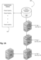
- Fig. 1A is a diagram illustrating an exemplary modeling system 100 used in accordance with embodiments described herein.
- the methods are tested and validated on a number of power systems 110, such as TCAs or HVAC systems of associated residential houses.
- an HVAC system includes the power system 110 that provides heat and/or air conditioning to the house, and also includes an associated meter for controlling the power system 110.
- a power system can also include other TCAs, such as water heaters and refrigerators.
- Consumption data such as actual one-minute HVAC consumption data is stored in a power consumption database 120.
- a power ETP model processor 130 uses power consumption data from the power consumption database 120, such as HVAC power consumption data and outdoor temperature data as inputs to estimate the parameters of the power ETP model.
- power consumption data from the power consumption database 120, such as HVAC power consumption data and outdoor temperature data.
- Algorithm 1 to estimate the parameters of the power ETP model is given in detail with reference to Fig. 4 .
- a power Decoupled-ETP model processor 140 is configured with circuitry to decouple the modeling of "ON” and “OFF” periods of a power unit to improve the modeling accuracy.
- power Decoupled-ETP model processor 140 is an HVAC Decoupled-ETP model processor.
- Algorithm 2 to decouple the modeling of "ON” and “OFF” periods is given in detail with reference to Fig. 10 .
- a power Adjusted Decoupled-ETP model processor 150 is configured with circuitry to derive the model parameters using only midnight data.
- power Adjusted Decoupled-ETP model processor 150 is an HVAC Adjusted Decoupled-ETP model processor. The method is applicable for cases in which the daytime power consumptions are heavily distorted by occupant activities.
- Algorithm 3 to decouple and adjust the model parameters is given in detail with reference to Fig. 14 .
- a prediction processor 160 is configured with circuitry to process and output a model used to forecast power unit behavior for energy management applications based upon one or more of the power ETP model processor 130, the power Decoupled-ETP model processor 140, and the power Adjusted Decoupled-ETP model processor 150.
- the model output uses outdoor temperature and HVAC power consumption data without knowledge of detailed parameters of the specific houses in which the HVAC units reside.
- Fig. 1A illustrates modeling system 100 as separate units. However, the processors described herein can be combined into one or more individual processing units, or other processing units not illustrated in Fig. 1 may be present.
- the processing units described in Fig. 1 encompass processing circuitry, either separately or as a combined whole that is configured to execute the process steps described herein.
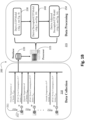
- Fig. 1B illustrates a second exemplary modeling system 200 for an HVAC system.
- a data collection module 210 illustrates devices in which data is collected, such as a thermometer 211 for each house and a thermostat 212 for each house.
- a data processing module 215 stores the data collected from the data collection module 210 in a data processing database 220. The retrieved data is processed via processor 225.
- Processor 225 could be a single processor or multiple processors running in parallel.
- Processor 225 derives the ETP model 230 as illustrated in Algorithm 1 in Fig. 4 .
- Processor 225 also derives the Decoupled-ETP model 240 as illustrated in Algorithm 2 in Fig. 10 .
- Processor 225 also derives the Adjusted Decoupled-ETP model 250 as illustrated in Algorithm 3 in Fig. 14 .
- Fig. 2 is a graph illustrating a first order HVAC ETP model.
- the indoor room temperature T room at t k
- 1 can be represented by the first order ETP model as
- T out remains constant, (1) can be rewritten as where t ON and t OFF refer to a complete ON and OFF cycle, as illustrated in Fig. 2 .
- a primary advantage of the first order ETP model for data-driven modeling is its simplicity.
- RCQ values can easily be derived from the set of five variables: T + , T, T out , t ON and t OFF .
- One disadvantage of the ETP model is that t ON and t OFF will change when T out changes.
- one set of RCQ values are needed to meet modeling accuracy requirements for each T out range.
- day-time and night-time RCQ values may not be the same, even though they are derived at the same T out because of solar radiation.
- one set of RCQ values can only be used for a T out range of 5-10°F for the nighttime portion of the day.
- a Decoupled-ETP model with a tuning method is described herein to resolve these modeling issues.
- the HVAC consumption, P ac can be converted to an on/off status u ac (t) based on
- the HVAC consumption, P ac , and the outdoor temperature, T out were collected by researchers in the PECAN street project. See Pecan Street Inc., "Dataport,”, 2017 , incorporated herein by reference in its entirety. One hundred houses were selected with one-minute sub-metered HVAC power consumption and outdoor temperature data. A summer time period time length was used in order to model an HVAC unit in its cooling mode.
- Fig. 3A is a graph illustrating a 48-hour HVAC power consumption curve.
- the first type of data is for midnight data from 12 a.m. to 5 a.m. when the activities of occupants that could influence the HVAC operations were at a minimum.
- Fig. 3B is a graph illustrating the 48-hour HVAC power consumption curve for the second type of data for 24-hr whole-day data in which occupants caused very little interference on HVAC operations.
- 3C is a graph illustrating the third type of data, which was discarded data in which the HVAC unit operation was either erratic or was frequently changing in an ON/OFF mode.
- the HVAC operation cannot be modeled appropriately by the RCQ parameter-based ETP model.
- Step 1 Input datasets for house i.
- Step 2. Convert P ac ( t ) to on/off status u ac ( f ) based on Equation (5).
- N ON,NIGHT ⁇ N ON,NIGHT,min e.g 5 min
- N OFF,NIGHT ⁇ N OFF,NIGHT,min e.g 5 min
- discard the data set e.g 5 min
- Step 7 If N ON,NIGHT ⁇ N ON,NIGHT,min (e.g 2 min) or N OFF,NIGHT ⁇ N OFF,NIGHT,min (e.g 5 min) or N ON,DAY ⁇ N ON,DAY,min (e.g 2 min) or N OFF,DAY ⁇ N OFF,DAY,min (e.g 5 min), discard the datasets. Step 7. Repeat Step 1 through Step 6 for all datasets in each house.
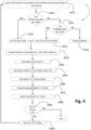
- Fig. 4 is a flowchart of Algorithm 1 illustrating process steps in an RCQ parameter estimation process for the first order ETP model of an HVAC unit.
- the process steps of Algorithm 1 can be implemented on a power ETP model processor 130 or other similar processor having circuitry configured to implement the process steps of Algorithm 1.
- An HVAC unit is described for illustrative purposes only.
- Other power units, such as a hot water heater and a refrigerator can also be incorporated with the process steps of Algorithm 1.
- step S410 HVAC power consumption data and ambient temperature data are input for a next house.
- Algorithm 1 is described using residential houses as the structure in which the power unit is located. However, other physical structures or buildings, such as business structures, commercial buildings, and warehouses can also be incorporated within Algorithm 400.
- step S420 it is determined whether whole-day data can be used. If whole-day data can be used (a "YES” decision in step S420), 24-hour data is selected in step S421. If whole-day data cannot be used (a "NO” decision in step S420, it is determined whether midnight data can be used in step S422. If midnight data can be used (a "YES” decision in step S422), 12:00 am to 5:00 am data is selected in step S423. If midnight data cannot be used (a "NO” decision in step S422), the dataset is discarded in step S424.
- step S430 the HVAC power consumption data is converted into HVAC status using Equation (5) where P ac,max is the maximum power consumption during t ⁇ and ⁇ is the set of total time horizon of input data; u ac is the HVAC status.
- a cycle vector S is calculated.
- the duration of each ON and OFF cycle, t ON and t OFF is calculated, as well as the corresponding average outdoor temperature T out_avg during each ON or OFF cycle.
- Each T out_avg was rounded to its nearest integer value.
- t ON (i), t OFF (i) and T out_avg were stored in the cycling characteristic vector, S(i) for the cycle i.
- an outdoor temperature can refer to a temperature outside of a physical structure in which the HVAC unit or other power unit is located.
- FIG. 5 is a graph illustrating an example of the cycling characteristic vector S matrix, which is also illustrated in Table I. Table I. An Example of Vector S S(i) S(1) S(2) S(3) S(4) S(5) S(6) ... t ON (i) NA 14 min NA 17 min NA 13 min ... t OFF (i) 10 min NA 11 min NA 15 min NA ... T out_avg ( i ) 85° F 85° F 89° F 89° F 84° F 81° F ...
- a median value of S is calculated to obtain vector M .
- the median values of t ON and t OFF were selected for each T out _ avg in S to obtain a new vector M.
- M was used to derive the correlation between ( t ON , t OFF ) and T out_avg when t ON or t OFF was missing for a certain T out_avg .
- the T out_avg was not included in M .
- An example of AV is illustrated in Table II.
- the outdoor temperature set in M was renamed as T o .
- the median value sets of t ON and t OFF were named as t ON M and t OFF M .
- FIG. 6A is a boxplot of the ON duration with respect to different outdoor temperatures.
- Fig. 6B is a boxplot of the OFF duration with respect to different values of T out , where T out is the outdoor temperature.
- Fig. 6C is a graph illustrating the median value of t ON M and t OFF M with respect to different outdoor temperatures. Table II.
- step S460 of Fig. 4 R, C, and Q parameters are calculated.
- T + and T were chosen to be 72°F and 68°F, respectively.
- Q is only a variable that influences the length of the HVAC ON cycle because in the OFF cycle, the room temperature decay is unrelated with the HVAC power consumption.
- Equation (6) and (7) it can be deduced that if the problem is treated as a curve fitting problem instead of considering the physical meanings of RCQ parameters, an arbitrary value can be selected for Q to calculate a corresponding set of values for A and C while the measured ON/OFF cycling characteristics can still be reproduced by the corresponding Decoupled-ETP model.
- step S470 unacceptable R, C, and Q sets are discarded.
- a bad set of RCQ values will fail to reproduce the HVAC cycling characteristic when T out varies from min( T o ) to max( T o ).
- the following two criteria are used to exclude the bad set of RCQ values obtained.
- Fig. 7A is a graph illustrating a set of RCQ values when Criterion A cannot be met.
- the physical meaning implies that the HVAC unit is undersized and it can no longer bring the room temperature down to T when the outdoor temperature is too high. Therefore, any set of RCQ values that violate the Criterion A need to be discarded.
- Fig. 7B is a graph illustrating the criterion A to ensure that when modeling the HVAC set point changes (e.g. [T , T + ] changes to [ T - , T + ]), t ON and t OFF will change accordingly.
- the HVAC set point changes e.g. [T , T + ] changes to [ T - , T + ]
- step S480 of Fig. 4 an optimum R, C , and Q set is selected.
- the best RCQ set (defined as R f , C f , and Q f obtained at outdoor temperature T f , wherein T f is a specific T out that generates R f , C f , and Q f ) in the N remaining sets can be selected by minimizing the error between the estimated and actual ON/OFF durations using min ⁇ T m ⁇ T o t ⁇ ON T ON ⁇ t ON M T ON 2 + t ⁇ OFF T OFF ⁇ t OFF M T OFF 2 where t ON (T out ) and t OFF (T out ) are the estimated ON and OFF durations under outdoor temperature T out calculated using equations (8) and (9); t ON M T out and t OFF M T out are the median value of ON/OFF durations under T out from actual measurements, which can be found in Vector M.
- An optimum R f C f Q f parameter set and a corresponding R f C f Q f parameter outdoor temperature, T f can be determined in which the converted power activated time cycles and the converted power non-activated time cycles match within a predefined margin of error actual power activated time cycles and actual power non-activated time cycles, respectively.
- FIG. 8 is a bar graph comparing the median of the measured ON/OFF durations, t N and t OFF M (ON,m and OFF,m in Fig. 8 ) and the estimated ON/OFF durations, t ON ⁇ M and t OFF ⁇ M (ON,e and OFF,e in Fig. 8 ) using the best R f C f Q f set.
- the R f C f Q f values were derived when the outdoor temperature was 84°F.
- step S485 it is determined whether the current house considered is the last house on a list of houses to be processed. If the current house is the last house (a "YES" decision in step S485), the process ends. If the current house is not the last house (a "NO” decision in step S485), a counter is used to go to the ( i + 1) th house in step S490. The process begins over at step S410 with the (i + 1) th house.
- the following exemplary algorithm may be used for selecting parameters for ETP HVAC models according to embodiments described herein.
- Step 1 Input S ON and sort S ON by T out .
- Equation (11) For each remaining set of R, C and Q after Step 5, calculate if Equation (11) is satisfied. If not, this set of R, C and Q will be discarded.
- Step 8 Repeat Step 1 through Step 7 for all houses.
- R f , C f can be obtained above.
- Fig. 9B is a graph illustrating linear correlation between Q and T out .
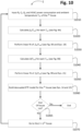
- Fig. 10 is a flow chart of Algorithm 2 for a Decoupled-ETP model.
- the process steps of Algorithm 2 can be implemented on a power Decoupled-ETP model processor 140 or other similar processor having circuitry configured to implement the process steps of Algorithm 2.
- step S 1010 R f , C f , Q f , and HVAC power consumption and ambient temperature T out of the i th house are input.
- Input parameters R f , C f , Q f are calculated as described herein with reference to step S480 in Fig. 4 .
- HVAC power consumption and ambient temperature T out are obtained from the HVAC consumption database 120 for the i th house.
- step S1020 f RC (T out ) is calculated.
- f RC T out ⁇ t OFF M / ln T out ⁇ T + T out ⁇ T ⁇ under each T out where T out , T off , and M are calculated from step S450 in Fig. 4
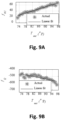
- Fig. 9A is a graph illustrating actual calculated results of f RC (T out ) for each T out .
- step S1030 a linear fit is performed of f RC (T out ) for each T out , an example of which is illustrated in Fig. 9A .
- Fig. 9B is a graph illustrating actual calculated results of Q(T out ) for each T out .
- step S 1050 a linear fit of Q ( T out ) is performed for each T out , an example of which is illustrated in Fig. 9B .
- step S 1060 a Decoupled-ETP model is built for the i th house.
- a ac k + 1 ⁇ 1 if T room k + 1 ⁇ T ⁇ 0 if T room k + 1 > T + u ac k else
- step S 1065 it is determined whether an end of a list of houses has been reached. If the end of the house list has been reached (a "YES” decision in step S1065), the process ends. If the end of the house list has not been reached (a "NO” decision in step S1065) the process continues to step S 1070.
- step S 1070 a counter increments to the (i + 1) th house and Algorithm 2 returns to step S 1010 to repeat the process for the next house.
- the following exemplary algorithm may be used for deriving the Decoupled-ETP model according to embodiments described herein.
- Step 7. Build the Decoupled ETP model based on Equations (14)-(15).
- Step 8. Repeat Step 1 through Step 7 for all datasets in each house.
- Fig. 11 is a bar graph illustrating a comparison between the estimated ON and OFF durations and the median of the actual ON/OFF durations with respect to outdoor temperature.
- the validation test for the one hundred houses was run using the PECAN street data set. The average errors between actual median of t ON and t OFF and the estimated t ⁇ ON and t ⁇ OFF were calculated. The average error among the one hundred houses over the full range of T out values was 4.02 and 2.05 minutes for the ETP model and the Decoupled-ETP model, respectively. If considering only the low (T out ⁇ 76°F) or the high ( T out >95°F) outdoor temperature cases, the modeling error of the Decoupled-ETP model is normally 10 ⁇ 20 minutes less than that of the ETP model.
- the Decoupled-ETP model can be applied to model all TCAs as long as the consumptions are regulated by a consistent thermostat setting without being distorted by activities of occupants, such as opening the doors or windows for a prolonged period, frequently changing thermostat set points, or manually shutting down the TCA devices, etc.
- TCA operations during daytime can heavily be distorted by human activities, as illustrated in Figs. 3A and 3C .
- the most usable data for deriving TCA models are the data measured between midnight and early morning when the occupants are asleep, such that the influence of their activities is a minimum.
- using only the midnight data can cause an inaccuracy since it does not account for the impact of solar radiations on the thermal dynamics of the house.
- an Adjusted Decoupled-ETP model is used to tune the parameters of the Decoupled-ETP model, which was derived using only the midnight data.
- the Adjusted Decoupled-ETP model the day-time operation can also be accurately modeled.
- R f,N , C f,N , f Q,N (T out ), and f RC,N (T out ) are the parameters of the Decoupled-ETP model calculated using the midnight data set.
- K R f , K C f , K Q (T out ) and K RC (T out ) are the adjustment coefficients for modeling daytime HVAC cycling behaviors.
- a NIGHT model and a WHOLE-DAY model represent the Decoupled-ETP model derived using the midnight data and the whole-day data, respectively.
- the NIGHT model parameters of the i lh HVAC unit include R ⁇ , N i , C ⁇ , N i , ⁇ Q , N i T out , and ⁇ RC , N i T out .
- the WHOLE-DAY model parameters include R ⁇ , D i , C ⁇ , D i , ⁇ Q , D i T out , and ⁇ RC , D i T out .
- the adjustment coefficients can be calculated as follows.
- K R f median R f , x 1 R f , x 1 , R f , x 2 R f , x 2 , ... , R f , x n R f , x n
- K C f median C f , x 1 C f , x 1 , C f , x 2 C f , x 2 , ... , C f , x n C f , x n K Q
- K Q T ax ⁇ k ⁇ Q ⁇ min T o + b ⁇ Q if T ax ⁇ min T o k ⁇ Q ⁇ T ax + b ⁇ Q if min T o ⁇ T ax ⁇ max T o k ⁇ Q ⁇ max T o + b ⁇ Q if T ax > min T o
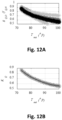
- Fig. 12A is a graph illustrating an example of g Q , D i T out ⁇ Q , N i T out when i ranges from 1 to 10 and K Q with respect to T out .
- Fig. 12B is a graph illustrating the linear fit model K ⁇ Q with respect to T out .
- K ⁇ SC T ax ⁇ a 0 ⁇ min T o 2 + a 1 ⁇ min T o + a 2 if T out ⁇ min T o a 0 ⁇ T out 2 + a 1 ⁇ T out + a 2 if min T o ⁇ T out ⁇ max T o a 0 ⁇ max T o 2 + a 1 ⁇ max T o + a 2 if T out > max T o
- Fig. 13A is a graph illustrating an example of ⁇ RC , D i T out ⁇ RC , N i T out when i ranges from 1 to 10 and K Q with respect to T out .
- Fig. 13B is a graph illustrating the second order polynomial model K ⁇ Q versus T out .
- the adjustment coefficients are derived, only the middle night data is used to derive the Decoupled-ETP model parameters.
- the NIGHT model parameters are adjusted using equations (28) and (29) so that when modeling the daytime HVAC cycling behaviors, the impact of solar radiation can be reflected appropriately.
- Fig. 14 is a flow chart of Algorithm 3 for the Adjusted Decoupled-ETP model.
- the process steps of Algorithm 3 can be implemented on a power Adjusted Decoupled-ETP model processor 150 or other similar processor having circuitry configured to implement the process steps of Algorithm 3.
- n non-distorted data is input.
- data can cover a 5-day, 24-hour period for household HVAC power consumption and ambient temperature data from the HVAC consumption database 120.
- Fig. 3B is a graph associated with Step 1 illustrating an acceptable HVAC consumption curve.
- step S1420 the midnight data is used to calculate the Decoupled-ETP model parameters for each household HVAC, R f , N 1 , C f , N 1 , f Q , N 1 T out , f SC , N 1 T out from estimations of Algorithm 2 (see Fig. 10 ).
- step S1430 whole-day data is used to calculate the Decoupled-ETP model parameters for each household HVAC, R 10 1 , C 10 1 , ⁇ 10 1 T m , ⁇ ⁇ , 1 T m from estimations of Algorithm 2 (see Fig. 10 ).
- step S 1450 a linear fit K Q (T out ) and a polynomial fit K RC (T out ) are performed.
- K ⁇ g T m ⁇ k ⁇ 0 ⁇ min T 0 + k ⁇ 0 if T m ⁇ min T 0 k ⁇ 0 ⁇ T m + k ⁇ 0 if min T 0 ⁇ T m ⁇ max T 0 k ⁇ 0 ⁇ max T 0 + k ⁇ 0 if T m > max T 0
- K ⁇ ⁇ T m ⁇ a 0 ⁇ min T 0 2 + a 1 ⁇ min T 0 + a 1 if T m ⁇ min T 0 a 0 ⁇ T m 2 + a 1 ⁇ T m + a 2 if min T 0 ⁇ T m ⁇ max T 0 a 0 ⁇ max T 0 + a 2 if min T 0 ⁇ T m
- step S 1460 an Adjusted Decoupled-ETP model is built for each HVAC unit.
- u m k + 1 ⁇ 1 if T mn k + 1 ⁇ T 0 if T mn k + 1 > T
- R ⁇ 1 K 1 ⁇ R 1
- the following exemplary algorithm may be used for deriving the Adjusted Decoupled-ETP model according to embodiments described herein.
- Step 1 Select at least N adj houses data ( P ac (t), T out ( t )) under the same season and repeat Algorithm 1 to select at least N S single family houses, N A apartments and N T townhouses that are capable to derive both Nighttime and Whole-day HVAC models.
- Step 3 Calculate adjustment gain K R f ,S , K C f ,S , K ⁇ Q,S ( T out ), K ⁇ RC,S (T out ) modified for single family data, s.
- Step 2 - Step 4 for selected N A apartments and obtain adjustment gain K R f ,A , K C f ,A , K Q,A ( T out ), K RC,A ( T out ) .
- Step 2 - Step 4 for selected N T townhouses and obtain adjustment gain K R f ,T , K C f ,T , K Q,T ( T out ), K RC,T ( T out ).
- Step 6 For each house to model, repeat Step 1 - Step 7 in Algorithm 2 and build the nighttime decoupled-ETP model with parameters R f N , C f N , Q f N , f RC N T out , f Q N T out .
- Step 7 Build the Adjusted Decoupled-ETP model using the following.
- Simulation results compared the performance of the ETP model with the Decoupled-ETP model and the Adjusted Decoupled-ETP model.
- Two performance criteria were used. The first criterion was the error in the measured and estimated total ON time durations and the second is the total number of switchings.
- the total ON duration reflects the accuracy of the model when estimating the total power consumptions.
- the total number of switchings indicates the accuracy of the model when estimating the switching behaviors.
- Table III shows the results comparing the errors in the total ON time and the total number of switchings when using the ETP model and the Decoupled-ETP model, respectively.
- APE is defined as the absolute percentage error.
- APE x ⁇ ⁇ x x where x is the actual measurement and x ⁇ is the estimation using the ETP model or the Decoupled ETP model. As illustrated in Table III, the performance of the Decoupled-ETP model is much better than the ETP model. Table III. Performance Comparison Total ON Time Total Switchings House #3192 Time (min) APE # times APE Actual 6788 NA 751 NA ETP Model 6471 4.66% 702 6.52% Decoupled ETP 6784 0.01% 766 2.00%
- Figs. 15A and 15B are bar graphs illustrating a mean absolute percentage error (MAPE) and a standard deviation (SD) of the total ON time based on night time data of one hundred HVAC units.
- the error distribution is for the ETP or the Decoupled-ETP model based on midnight data.
- Figs. 15C and 15D are bar graphs illustrating MAPE and a SD of the total number of switchings of one hundred HVAC units. Table IV also illustrates these results.
- the results illustrate the total ON time and the total number of switchings of the Decoupled-ETP model have a much lower MAPE and SD than those of the ETP model.
- the performance of the ETP model, the Decoupled-ETP model, and the Adjusted Decoupled-ETP model was verified using 24-hour whole day data, as illustrated below.
- the performance of the Adjusted Decoupled-ETP models was verified using House #3456 data and verification results using 50 HVAC units.
- Table V illustrates the comparison of errors in the total ON time and the number of switchings for different models. Table V. Results Comparison, House #3456 at Austin, Texas from 15:18 pm July 12 th to 21:57 pm August 2 nd . 2015 Total ON Time Total Switchings House #3456 Data Input Time (min) APE # Times APE Actual NA 5779 NA 669 NA ETP1 Midnight 11713 102.68% 946 41.30% ETP2 Whole day 5487 5.05% 583 12.86% Decoupled-ETP 1 Midnight 6338 9.68% 733 9.62% Decoupled-ETP2 Whole day 5765 0.25% 335 0.10% Adjusted Decoupled-ETP Midnight 6152 6.46% 708 5.77%
- Data Input refers to the type of data that was used to build the model.
- the Whole-day data used the 24-hr consumption of the HVAC unit in house #3456 as inputs and the Night data used 12 a.m. to 5 am. HVAC consumption as inputs.
- the Decoupled-ETP model using the whole-day data as inputs had the best performance with the lowest errors. When the midnight model was used without being adjusted, the modeling error increased sharply. When using the Adjusted Decoupled-ETP model, the error was reduced by close to 50%.
- the error was defined as the cumulated error of 21 days, the average daily modeling errors in the total ON time were within 18 minutes and the average errors in modeling the number of switches were within two times. This illustrates an improved performance when modeling the HVAC switching characteristics
- Figs. 16A through 16F verify the Case 1 results using data collected from fifty houses during summer months.
- Figs. 16A and 16B are bar graphs illustrating ON time APE and Switching APE, respectively for the Decoupled-ETP1 model.
- Figs. 16C and 16D are bar graphs illustrating ON time APE and Switching APE, respectively for the Decoupled-ETP2 model.
- Figs. 16E and 16F are bar graphs illustrating ON time APE and Switching APE, respectively for the Adjusted Decoupled-ETP model. The results show that all three Decoupled-ETP model performances were consistent across households. If only the midnight data is usable, the Adjusted Decoupled-ETP model can be used for modeling the day-time HVAC behaviors.
- Previous systems and methods have attempted to reduce peak power by controlling generators, thermostats, etc. based on a centralized system model, architecture, or configuration.
- Some systems and methods have modeled uncertainties in aggregated HVAC loads using a state queueing model, wherein no control is involved.
- Other methods reshape the energy demand profile of aggregated buildings, which is also based on a centralized system design and model.
- One HVAC aggregated model is based on an ETP model and a centralized control strategy.
- Other systems and methods use an HVAC load control strategy to follow the targeted load curve, which is based on a centralized multi-objective system model, architecture, or configuration.
- Still other systems and methods use a state space-based HVAC simulation model based on an ETP model, wherein no control is involved.
- embodiments herein describe data-driven methods and models to estimate the ETP model parameters of TCAs using their power consumptions and ambient temperature data as inputs.
- the modeling of HVAC units is used to decouple the modeling of the ON and OFF cycles, which simplifies the derivation of modeling parameters and significantly improves the modeling accuracy.
- midnight data is used for ETP model parameter estimation.
- a tuning process is used to adjust the nighttime models due to the impact of solar radiation.
- the functions and processes of the modeling system 100 can be implemented in part by a computer 1700 illustrated in Fig. 17 .
- power consumption database 120, power ETP model processor 130, power Decoupled-ETP model processor 140, power Adjusted Decoupled-ETP model processor 150, and/or prediction processor 160 con be implemented by the computer 1700, either separately or together as one or more units.
- the computer 1700 includes a CPU 1701 which performs the processes described herein.
- the process data and instructions may be stored in memory 1702.
- These processes and instructions may also be stored on a storage medium disk 1704 such as a hard drive (HDD) or portable storage medium or may be stored remotely.
- a storage medium disk 1704 such as a hard drive (HDD) or portable storage medium or may be stored remotely.
- the claimed advancements are not limited by the form of the computer-readable media on which the instructions of the inventive process are stored.
- the instructions may be stored on CDs, DVDs, in FLASH memory, RAM, ROM, PROM, EPROM, EEPROM, hard disk or any other information processing device with which the computer 1700 communicates, such as a server or computer.
- claimed advancements may be provided as a utility application, background daemon, or component of an operating system, or combination thereof, executing in conjunction with CPU 1701 and an operating system such as Microsoft ® Windows ® , UNIX ® , Oracle ® Solaris, LINUX ® , Apple macOS ® and other systems known to those skilled in the art.
- an operating system such as Microsoft ® Windows ® , UNIX ® , Oracle ® Solaris, LINUX ® , Apple macOS ® and other systems known to those skilled in the art.
- CPU 1701 may be a Xenon ® or Core ® processor from Intel Corporation of America or an Opteron ® processor from AMD of America, or may be other processor types that would be recognized by one of ordinary skill in the art.
- the CPU 1701 may be implemented on an FPGA, ASIC, PLD or using discrete logic circuits, as one of ordinary skill in the art would recognize Further, CPU 1701 may be implemented as multiple processors cooperatively working in parallel to perform the instructions of the inventive processes described above.
- the computer 1700 in Fig. 17 also includes a network controller 1706, such as an Intel Ethernet PRO network interface card from Intel Corporation of America, for interfacing with network 1724.
- the network 1724 can be a public network, such as the Internet, or a private network such as LAN or WAN network, or any combination thereof and can also include PSTN or ISDN sub-networks.
- the network 1724 can also be wired, such as an Ethernet network, or can be wireless such as a cellular network including EDGE, 3G and 4G wireless cellular systems.
- the wireless network can also be WiFi ® , Bluetooth ® , or any other wireless form of communication that is known.
- the computer 1700 further includes a display controller 1708, such as a NVIDIA ® GeForce ® GTX or Quadro ® graphics adaptor from NVIDIA Corporation of America for interfacing with display 1710, such as a Hewlett Packard ® HPL2445w LCD monitor.
- a general purpose I/O interface 1712 interfaces with a keyboard and/or mouse 1714 as well as an optional touch screen panel 1716 on or separate from display 1710.
- General purpose I/O interface 1712 also connects to a variety of peripherals 1718 including printers and scanners, such as an OfficeJet ® or DeskJet ® from Hewlett Packard.
- the general purpose storage controller 1720 connects the storage medium disk 1704 with communication bus 1722, which may be an ISA, EISA, VESA, PCI, or similar, for interconnecting all of the components of the computer 1700.
- communication bus 1722 which may be an ISA, EISA, VESA, PCI, or similar, for interconnecting all of the components of the computer 1700.
- a description of the general features and functionality of the display 1710, keyboard and/or mouse 1714, as well as the display controller 1708, storage controller 1720, network controller 1706, and general purpose I/O interface 1712 is omitted herein for brevity as these features are known.
Landscapes
- Engineering & Computer Science (AREA)
- Business, Economics & Management (AREA)
- Physics & Mathematics (AREA)
- General Physics & Mathematics (AREA)
- Economics (AREA)
- Health & Medical Sciences (AREA)
- Tourism & Hospitality (AREA)
- Human Resources & Organizations (AREA)
- Strategic Management (AREA)
- Signal Processing (AREA)
- Marketing (AREA)
- Mechanical Engineering (AREA)
- General Engineering & Computer Science (AREA)
- General Business, Economics & Management (AREA)
- Combustion & Propulsion (AREA)
- Theoretical Computer Science (AREA)
- Chemical & Material Sciences (AREA)
- Primary Health Care (AREA)
- General Health & Medical Sciences (AREA)
- Power Engineering (AREA)
- Water Supply & Treatment (AREA)
- Public Health (AREA)
- Fuzzy Systems (AREA)
- Mathematical Physics (AREA)
- Computer Vision & Pattern Recognition (AREA)
- Artificial Intelligence (AREA)
- Evolutionary Computation (AREA)
- Medical Informatics (AREA)
- Software Systems (AREA)
- Automation & Control Theory (AREA)
- Entrepreneurship & Innovation (AREA)
- Operations Research (AREA)
- Quality & Reliability (AREA)
- Game Theory and Decision Science (AREA)
- Development Economics (AREA)
- Air Conditioning Control Device (AREA)
- Control Of Resistance Heating (AREA)
Description
- Thermostatically controlled appliances (TCA) such as heating, ventilation, and air conditioning (HVAC) units, and water heaters are commonly used as load-side resources for demand response programs and home energy management (HEM) systems. To control the electricity consumption of a TCA unit without tempering user comfort, an equivalent thermal parameter (ETP) model of the TCA unit is normally needed to forecast the ON/OFF status of the unit for a few hours. The ETP model uses the thermostat set point, outdoor temperature, and an initial room temperature as inputs to predict the subsequent ON/OFF cycles.
- In Ruzzelli et al. load detection methods are proposed based on signal processing methods such as signal extraction, neural networks, spectrum analysis, V-I trajectory, and wavelet transforms. However, these methods are used for detecting the loads instead of deriving a model that can forecast the load behaviors in subsequent intervals. See A. G. Ruzzelli, C. Nicolas, A. Schoofs and G. M. P. O'Hare, "Real-Time Recognition and Profiling of Appliances through a Single Electricity Sensor," 2010 7th Annual IEEE Communications Society Conference on Sensor, Mesh and Ad Hoc Communications and Networks (SECON), Boston, MA, 2010, pp. 1-9; S. Makonin, F. Popowich, L. Bartram, B. Gill and I. V. Bajić, "AMPds: A public dataset for load disaggregation and eco-feedback research," 2013 IEEE Electrical Power & Energy Conference, Halifax, NS, 2013, pp. 1-6; M. Weiss, A. Helfenstein, F. Mattern and T. Staake, "Leveraging smart meter data to recognize home appliances," 2012 IEEE International Conference on Pervasive Computing and Communications, Lugano, 2012, pp. 190-197; M. Dong, P. C. M. Meira, W. Xu and C. Y. Chung, "Non-Intrusive Signature Extraction for Major Residential Loads," in IEEE Transactions on Smart Grid, vol. 4, no. 3, pp. 1421-1430, Sept. 2013; A. I. Cole and A. Albicki, "Data extraction for effective non-intrusive identification of residential power loads," 1MTC/98 Conference Proceedings. IEEE Instrumentation and Measurement Technology Conference. St. Paul, MN, 1998, pp. 812-815 vol.2; and H. Najmeddine et al., "State of art on load monitoring methods," 2008 IEEE 2nd International Power and Energy Conference, Johor Bahru, 2008, pp. 1256-1258, each incorporated herein by reference in their entireties.
- For residential applications, researchers normally apply first or second order differential equations to represent the thermal dynamics of a single-family household when outdoor temperature changes. See S. Katipamula and N. Lu, "Evaluation of residential HVAC control strategies for demand response programs," ASHRAE Trans., vol. 1, no. 12, pp. 1-12, 2006, incorporated herein by reference in its entirety. The ETP model parameters are derived from a physics-based approach or a measurement-based approach.
- The physics-based methods usually model the house in detail. See S. Shao, M. Pipattanasomporn and S. Rahman, "Development of physical-based demand response-enabled residential load models," in IEEE Transactions on Power Systems, vol. 28, no. 2, pp. 607-614, May 2013; S. Ihara and F. C. Schweppe, "Physically based modeling of cold load pickup," IEEE Trans. Power App. Syst., vol. PAS-100, no. 9, pp. 4142-4150, Sep. 1981; E. Agneholm and J. Daalder, "Cold load pick-up of residential load," Proc. Inst. Elect. Eng., Gen., Transm.,Distrib., vol. 147, no. 1, pp.44-50, Jan. 2000; J. Yan, Q. Zeng, Y. Liang, L. He and Z. Li, "Modeling and Implementation of Electroactive Smart Air-Conditioning Vent Register for Personalized HVAC Systems," in IEEE Access, to be published, doi: 10.1109/ACCESS.2017.2664580; A. Gomes, C. H. Antunes, and A. G. Martins, "Physically-based load demand models for assessing electric load control actions," in Proc. IEEE Bucharest PowerTech, Jul. 2009; and R. E.Mortensen and K. P. Haggerty, "A stochastic computer model for heating and cooling loads," IEEE Trans. Power Syst., vol. 3, no. 3, pp. 1213-1219, Aug. 1988, each incorporated herein by reference in their entireties. The inputs include the material and thickness of the walls, the size and number of windows, the thermal mass in the houses, the facing of the house, etc. This type of approach is usually used for modeling a typical residential house. When modeling an actual house for the HEM control purpose, it is impractical because many unforeseeable factors, such as construction material variations, tree covers, and vent locations can have a significant impact on the accuracy of the model.
- Measurement-based methods have been used to overcome some of the deficiencies of physics-based methods to derive the ETP parameters. In Lu, N. Lu proposed a data-driven HVAC model in which the parameters are derived from curve-fitting the HVAC consumption curves. See N. Lu, "An evaluation of the HVAC load potential for providing load balancing service," IEEE Trans. Smart Grid, vol. 3, no. 3, pp. 1263-1270, Sep. 2012, incorporated herein by reference in its entirety. To account for the impact of outdoor temperature, an adjustment can be made using a look-up table that contains a set of HVAC parameters under each temperature range. However, this data-driven model was derived and tested primarily using the HVAC consumption data produced by higher-order physics-based ETP models because sub-metered high-resolution HVAC consumption data was not available. The accuracy of the model was not satisfactory during validation using metered one-minute HVAC consumptions.
-
US2013/0282181 discloses controlling aggregated thermostatically controlled appliances for demand response with a separated calculation for ON and OFF periods based on time lapse. However, heat flow parameters are not calculated. - The "background" description provided herein is for the purpose of generally presenting the context of the disclosure. Work of the presently named inventors, to the extent it is described in this background section, as well as aspects of the description which may not otherwise qualify as conventional at the time of filing, are neither expressly nor impliedly admitted as conventional against the present disclosure.
- Embodiments described herein include the following aspects.
- (1) A method of improving an energy parameter estimation includes storing power consumption data retrieved from a plurality of power systems into a power consumption database; converting, via processing circuitry, the power consumption data into power activated time cycles and power non-activated time cycles; calculating, via the processing circuitry, median time values of the power activated time cycles and the power non-activated time cycles for respective outdoor temperatures; deriving a thermal resistance (R) parameter and a capacitance (C) parameter for a predetermined heat flow (Q) parameter at each of the respective outdoor temperatures for the plurality of power systems; comparing, via the processing circuitry, the converted power activated time cycles to the actual power activated time cycles for the plurality of power systems; comparing, via the processing circuitry, the converted power non-activated time cycles to the actual power non-activated time cycles for the plurality of power systems; calculating a first improved resistance-capacitance-heat flow (RCQ) parameter set and a respective first outdoor temperature for the compared and converted power activated time cycles to the actual power activated time cycles; calculating a second improved RCQ parameter set and a respective second outdoor temperature for the compared and converted power non-activated time cycles to the actual power non-activated time cycles; and improving the energy parameter estimation by executing the first and second improved RCQ parameter sets at the respective first and second outside temperatures for each of the plurality of power systems, wherein the improving the energy parameter estimation identifies energy efficiencies to reduce a total energy load within said each of the plurality of power systems.
- (2) The method of improving an energy parameter estimation of (1), wherein the improved RCQ parameter set is determined by minimizing an error between the converted power activated time cycles and the actual power activated time cycles, and between the converted power non-activated time cycles and the actual power non-activated time cycles.
- (3) The method of improving an energy parameter estimation of either (1) or (2), wherein the power consumption data is limited to data within a temperature range between a predefined upper limit temperature and a predefined lower limit temperature.
- (4) The method of improving an energy parameter estimation of any one of (1) through (3), wherein the method comprises an equivalent thermal parameter (ETP) model for improving the energy parameter estimation.
- (5) The method of improving an energy parameter estimation of any one of (1) through (4), further includes calculating the Q parameter at each of the respective outdoor temperatures during the power activated time cycles for the plurality of power systems; and calculating the R parameter and the C parameter at each of the respective outdoor temperatures during the power non-activated time cycles for the plurality of power systems.
- (6) The method of improving an energy parameter estimation of any one of (1) through (5), further includes calculating, via the processing circuitry, an estimated duration of each of the power activated time cycles from the Q parameter calculated at each of the respective outdoor temperatures; calculating, via the processing circuitry, an estimated duration of each of the power non-activated time cycles from the R parameter and the C parameter calculated at each of the respective outdoor temperatures; and improving the energy parameter estimation to reduce errors corresponding to variations in said each of the respective outdoor temperatures by decoupling daytime parameters from night time parameters via the estimated duration of said each of the power activated time cycles from the Q parameter and via the estimated duration of said each of the power non-activated time cycles from the R parameter and the C parameter.
- (7) The method of improving an energy parameter estimation of any one of (1) through (6), further includes calculating an R adjustment coefficient as a ratio of a whole-day R parameter to a night-time R parameter; calculating a C adjustment coefficient as a ratio of a whole-day C parameter to a night-time C parameter; calculating a Q adjustment coefficient at said each of the respective outdoor temperatures as a ratio of a whole-day Q parameter to a night-time Q parameter at said each of the respective outdoor temperatures; and calculating an RC adjustment coefficient at said each of the respective outdoor temperatures as a ratio of a whole-day RC parameter to a night-time RC parameter at said each of the respective outdoor temperatures; wherein the whole-day R parameter, the whole-day C parameter, the whole-day Q parameter, and the whole-day RC parameter are calculated from data taken over a 24-hour period of time, and wherein the night-time R parameter, the night-time C parameter, the night-time Q parameter, and the night-time RC parameter are calculated from data taken during an absence of solar exposure.
- (8) The method of improving an energy parameter estimation of any one of (1) through (7), further includes calculating a daytime R parameter as a product of the R adjustment coefficient and a night-time optimum R parameter; calculating a daytime C parameter as a product of the C adjustment coefficient and a night-time optimum C parameter; calculating a daytime Q parameter as a product of the Q adjustment coefficient and a night-time optimum Q parameter at said each of the respective outdoor temperatures; calculating a daytime RC parameter as a product of the RC adjustment coefficient and a night-time optimum RC parameter at said each of the respective outdoor temperatures; and improving the energy parameter estimation to reduce errors corresponding to variations in solar exposure by adjusting night time parameters to be used as daytime parameters via the daytime R parameter, the daytime C parameter, the daytime Q parameter, and the daytime RC parameter.
- (9) The method of improving an energy parameter estimation of any one of (1) through (8), wherein the plurality of power systems includes a plurality of thermostatically controlled appliances (TCAs).
- (10) The method of improving an energy parameter estimation of any one of (1) through (9), wherein the plurality of TCAs includes a plurality of heating, ventilation, and air conditioning (HVAC) systems, and the power consumption database includes an HVAC consumption database.
- (11) A decoupled equivalent thermal parameter (ETP) model processor includes circuitry. The circuitry is configured to store power consumption data retrieved from a plurality of power systems into a power consumption database; convert the power consumption data into power activated time cycles and power non-activated time cycles; calculate median time values of the power activated time cycles and the power non-activated time cycles for respective outdoor temperatures; derive parameters for a thermal resistance (R) parameter and a capacitance (C) parameter for a predetermined heat flow (Q) parameter at each of the respective outdoor temperatures for the plurality of power systems; compare the converted power activated time cycles to the actual power activated time cycles for the plurality of power systems; compare the converted power non-activated time cycles to the actual power non-activated time cycles for the plurality of power systems; calculate a first improved resistance-capacitance-heat flow (RCQ) parameter set and a respective first outdoor temperature for the compared and converted power activated time cycles to the actual power activated time cycles; calculate a second improved RCQ parameter set and a respective second outdoor temperature for the compared and converted power non-activated time cycles to the actual power non-activated time cycles; calculate the Q parameter at each of the respective outdoor temperatures during the power activated time cycles for the plurality of power systems; and calculate the R parameter and the C parameter at each of the respective outdoor temperatures during the power non-activated time cycles for the plurality of power systems.
- (12) The decoupled ETP model processor of (11), wherein the circuitry is further configured to calculate an estimated duration of each of the power activated time cycles from the Q parameter calculated at each of the respective outdoor temperatures; and calculate an estimated duration of each of the power non-activated time cycles from the R parameter and the C parameter calculated at each of the respective outdoor temperatures; wherein the calculated Q parameter, the calculated R parameter, and the calculated C parameter improve energy parameter estimation to reduce errors corresponding to variations in said each of the respective outdoor temperatures by decoupling daytime parameters from night time parameters via the estimated duration of said each of the power activated time cycles from the Q parameter and via the estimated duration of said each of the power non-activated time cycles from the R parameter and the C parameter.
- (13) The decoupled ETP model processor of either (11) or (12), wherein the improved RCQ parameter set is determined by minimizing an error between the converted power activated time cycles and the actual power activated time cycles, and between the converted power non-activated time cycles and the actual power non-activated time cycles.
- (14) The decoupled ETP model processor of any one of (11) through (13), wherein the plurality of power systems includes a plurality of thermostatically controlled appliances (TCAs).
- (15) An adjusted decoupled ETP model processor includes circuitry. The circuitry is configured to store power consumption data retrieved from a plurality of power systems into a power consumption database; convert the power consumption data into power activated time cycles and power non-activated time cycles; calculate median time values of the power activated time cycles and the power non-activated time cycles for respective outdoor temperatures; derive parameters for a thermal resistance (R) parameter and a capacitance (C) parameter for a predetermined heat flow (Q) parameter at each of the respective outdoor temperatures for the plurality of power systems; compare the converted power activated time cycles to the actual power activated time cycles for the plurality of power systems; compare the converted power non-activated time cycles to the actual power non-activated time cycles for the plurality of power systems; calculate a first improved resistance-capacitance-heat flow (RCQ) parameter set and a respective first outdoor temperature for the compared and converted power activated time cycles to the actual power activated time cycles; calculate a second improved RCQ parameter set and a respective second outdoor temperature for the compared and converted power non-activated time cycles to the actual power non-activated time cycles; calculate an R adjustment coefficient as a ratio of a whole-day R parameter to a night-time R parameter; calculate a C adjustment coefficient as a ratio of a whole-day C parameter to a night-time C parameter; calculate a Q adjustment coefficient at the respective outdoor temperature as a ratio of a whole-day Q parameter at the respective outdoor temperature to a night-time Q parameter at the respective outdoor temperature; and calculate an RC adjustment coefficient at the respective outdoor temperature as a ratio of a whole-day RC parameter at the respective outdoor temperature to a night-time RC parameter at the respective outdoor temperature.
- (16) The adjusted decoupled ETP model processor of (15), wherein the circuitry is further configured to calculate a daytime R parameter as a product of the R adjustment coefficient and a night-time optimum R parameter; calculate a daytime C parameter as a product of the C adjustment coefficient and a night-time optimum C parameter; calculate a daytime Q parameter as a product of the Q adjustment coefficient and a night-time optimum Q parameter at the respective outdoor temperature; and calculate a daytime RC parameter as a product of the RC adjustment coefficient and a night-time optimum RC parameter at said each of the respective outdoor temperatures; wherein the calculated daytime R parameter, the calculated daytime C parameter, the calculated daytime Q parameter, and the calculated daytime RC parameter improve energy parameter estimation to reduce errors corresponding to variations in solar exposure by adjusting night time parameters to be used as daytime parameters.
- (17) The adjusted decoupled ETP model processor of either (15) or (16), wherein the whole-day R parameter, the whole-day C parameter, the whole-day Q parameter, and the whole-day RC parameter are calculated from data taken over a 24-hour period of time, and wherein the night-time R parameter, the night-time C parameter, the night-time Q parameter, and the night-time RC parameter are calculated from data taken during an absence of solar exposure.
- (18) The adjusted decoupled ETP model processor of any one of (15) through (17), wherein the improved RCQ parameter set is determined by minimizing an error between the converted power activated time cycles and the actual power activated time cycles, and between the converted power non-activated time cycles and the actual power non-activated time cycles.
- (19) The adjusted decoupled ETP model processor of any one of (15) through (18), wherein the plurality of power systems includes a plurality of thermostatically controlled appliances (TCAs).
- (20) The adjusted decoupled ETP model processor of any one of (15) through (19), wherein the plurality of TCAs includes a plurality of heating, ventilation, and air conditioning (HVAC) systems, and the power consumption database includes an HVAC consumption database.
- The foregoing paragraphs have been provided by way of general introduction, and are not intended to limit the scope of the following claims. The described embodiments, together with further advantages, will be best understood by reference to the following detailed description taken in conjunction with the accompanying drawings.
- A more complete appreciation of the invention and many of the attendant advantages thereof will be readily obtained as the same becomes better understood by reference to the following detailed description when considered in connection with the accompanying drawings, wherein:
-
Fig. 1A is a diagram illustrating an exemplary modeling system according to one embodiment; -
Fig. 1B illustrates a second exemplary modeling system for an HVAC system according to one embodiment; -
Fig. 2 is a graph illustrating an output based on a first order HVAC ETP model according to one embodiment; -
Fig. 3A is a graph illustrating a first type of data for midnight data according to one embodiment; -
Fig. 3B is a graph illustrating a second type of data for 24-hr whole-day data according to one embodiment; -
Fig. 3C is a graph illustrating a third type of data, which is discarded data according to one embodiment; -
Fig. 4 is a flowchart ofAlgorithm 1 illustrating six steps in an RCQ parameter estimation process for the first order ETP model according to one embodiment; -
Fig. 5 is a graph illustrating an example of the cycling characteristic vector S matrix according to one embodiment; -
Fig. 6A is a boxplot of the ON duration with respect to different outdoor temperatures (Tout ) according to one embodiment; -
Fig. 6B is a boxplot of the OFF duration with respect to different outdoor temperatures according to one embodiment; -
Fig. 6C is a graph illustrating the median value of


-
Fig. 7A is a graph illustrating a set of RCQ values when Criterion A cannot be met, where R represents thermal resistance, C represents thermal capacitance, and Q represents heat flow according to one embodiment; -
Fig. 7B is a graph illustrating the criterion to ensure that when modeling the HVAC set point changes, tON and tOFF will change according to one embodiment; -
Fig. 8 is a bar graph comparing the median of the measured ON/OFF durations,


-
Fig. 9A is a graph illustrating linear correlation between R×C and Tout according to one embodiment; -
Fig. 9B is a graph illustrating linear correlation between Q and Tout according to one embodiment; -
Fig. 10 is a flow chart ofAlgorithm 2 of a Decoupled-ETP model according to one embodiment; -
Fig. 11 is a bar graph illustrating a comparison between the estimated ON and OFF durations and the median of the actual ON/OFF durations with respect to outdoor temperature according to one embodiment; -
Fig. 12A is a graph illustrating an example of
-
Fig. 12B is a graph illustrating the linear fit model K̃Q with respect to Tout according to one embodiment; -
Fig. 13A is a graph illustrating an example of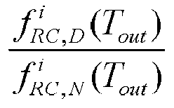
-
Fig. 13B is a graph illustrating a second order polynomial model K̃Q versus Tout according to one embodiment; -
Fig. 14 is a flow chart ofAlgorithm 3 for an Adjusted Decoupled-ETP model according to one embodiment; -
Figs. 15A and 15B are bar graphs illustrating a mean absolute percentage error (APE) and a standard deviation (SD) of the total ON time based on night time data according to one embodiment; -
Figs. 15C and 15D are bar graphs illustrating an APE and a SD of the total number of switchings according to one embodiment; -
Figs. 16A and 16B are bar graphs illustrating ON time APE and Switching APE, respectively for a Decoupled-ETP 1 model according to one embodiment; -
Figs. 16C and16D are bar graphs illustrating ON time APE and Switching APE, respectively for a Decoupled-ETP2 model according to one embodiment; -
Figs. 16E and 16F are bar graphs illustrating ON time APE and Switching APE, respectively for an Adjusted Decoupled-ETP model according to one embodiment; and -
Fig. 17 is a block diagram illustrating a hardware description of a computer according to one embodiment. - The following descriptions are meant to further clarify the present disclosure by giving specific examples and embodiments of the disclosure. These embodiments are meant to be illustrative rather than exhaustive. The full scope of the disclosure is not limited to any particular embodiment disclosed in this specification, but rather is defined by the claims.
- It will be appreciated that in the development of any such actual implementation, numerous implementation-specific decisions need to be made in order to achieve the developer's specific goals, such as compliance with application- and business-related constraints, and that these specific goals will vary from one implementation to another and from one developer to another.
- A data-driven, decoupled modeling method for deriving model parameters of thermostatically controlled appliances (TCAs) is described herein using a heating, ventilation, and air conditioning (HVAC) unit as an example. The method uses outdoor temperature and HVAC power consumption as inputs to estimate the parameters of the HVAC equivalent thermal parameter (ETP) model.
- An HVAC is used as an example to illustrate model parameter estimation processes and adjustment algorithms. Residential households are used as a primary focus herein. Therefore, models of HVAC units with variable frequency drives are not considered. However, adjustments can be made to incorporate the embodiments described herein to HVAC units with variable frequency drives. In addition, the methods and systems described herein can easily be extended to a parameter estimation of many other thermostatically controlled appliances (TCAs), such as water heaters and refrigerators.
-
Fig. 1A is a diagram illustrating anexemplary modeling system 100 used in accordance with embodiments described herein. The methods are tested and validated on a number ofpower systems 110, such as TCAs or HVAC systems of associated residential houses. For example, an HVAC system includes thepower system 110 that provides heat and/or air conditioning to the house, and also includes an associated meter for controlling thepower system 110. A power system can also include other TCAs, such as water heaters and refrigerators. Consumption data, such as actual one-minute HVAC consumption data is stored in apower consumption database 120. - A power
ETP model processor 130 uses power consumption data from thepower consumption database 120, such as HVAC power consumption data and outdoor temperature data as inputs to estimate the parameters of the power ETP model. A description ofAlgorithm 1 to estimate the parameters of the power ETP model is given in detail with reference toFig. 4 . - A power Decoupled-
ETP model processor 140 is configured with circuitry to decouple the modeling of "ON" and "OFF" periods of a power unit to improve the modeling accuracy. In an example, power Decoupled-ETP model processor 140 is an HVAC Decoupled-ETP model processor. A description ofAlgorithm 2 to decouple the modeling of "ON" and "OFF" periods is given in detail with reference toFig. 10 . - A power Adjusted Decoupled-ETP model processor 150 is configured with circuitry to derive the model parameters using only midnight data. In an example, power Adjusted Decoupled-ETP model processor 150 is an HVAC Adjusted Decoupled-ETP model processor. The method is applicable for cases in which the daytime power consumptions are heavily distorted by occupant activities. A description of
Algorithm 3 to decouple and adjust the model parameters is given in detail with reference toFig. 14 . - A
prediction processor 160 is configured with circuitry to process and output a model used to forecast power unit behavior for energy management applications based upon one or more of the powerETP model processor 130, the power Decoupled-ETP model processor 140, and the power Adjusted Decoupled-ETP model processor 150. For example, the model output uses outdoor temperature and HVAC power consumption data without knowledge of detailed parameters of the specific houses in which the HVAC units reside. -
Fig. 1A illustratesmodeling system 100 as separate units. However, the processors described herein can be combined into one or more individual processing units, or other processing units not illustrated inFig. 1 may be present. The processing units described inFig. 1 encompass processing circuitry, either separately or as a combined whole that is configured to execute the process steps described herein. -
Fig. 1B illustrates a secondexemplary modeling system 200 for an HVAC system. Adata collection module 210 illustrates devices in which data is collected, such as athermometer 211 for each house and athermostat 212 for each house. - A
data processing module 215 stores the data collected from thedata collection module 210 in adata processing database 220. The retrieved data is processed viaprocessor 225.Processor 225 could be a single processor or multiple processors running in parallel.Processor 225 derives theETP model 230 as illustrated inAlgorithm 1 inFig. 4 .Processor 225 also derives the Decoupled-ETP model 240 as illustrated inAlgorithm 2 inFig. 10 .Processor 225 also derives the Adjusted Decoupled-ETP model 250 as illustrated inAlgorithm 3 inFig. 14 . -
Fig. 2 is a graph illustrating a first order HVAC ETP model. For a current time step of t=k, the indoor room temperature Troom at t=k | 1 can be represented by the first order ETP model as
- where Tout and Troom are the outdoor and room temperature, respectively, uac is the HVAC ON/OFF status, Δt is the duration of each time step, R represents thermal resistance, C represents thermal capacitance, and Q represents the heat flow provided by the HVAC unit. Therefore, the HVAC status uac at the next
time step k+ 1 can be determined by
- where T - and T + refer to the lower and upper bounds of the HVAC temperature deadband, respectively. A predefined upper limit temperature and a predefined lower limit temperature can be established according to specific process objectives, equipment limitations, etc. For example, the predefined upper limit temperature can be the upper temperature of an indoor comfort zone such as 72° F, while the predefined lower limit temperature can be the lower temperature of the indoor comfort zone such as 68° F.
- If Tout remains constant, (1) can be rewritten as


Fig. 2 . - A primary advantage of the first order ETP model for data-driven modeling is its simplicity. RCQ values can easily be derived from the set of five variables: T +, T, Tout, tON and tOFF. One disadvantage of the ETP model is that tON and tOFF will change when Tout changes. As a result, one set of RCQ values are needed to meet modeling accuracy requirements for each Tout range. In addition, day-time and night-time RCQ values may not be the same, even though they are derived at the same Tout because of solar radiation. For example, one set of RCQ values can only be used for a Tout range of 5-10°F for the nighttime portion of the day. A Decoupled-ETP model with a tuning method is described herein to resolve these modeling issues.
- The HVAC consumption, Pac, can be converted to an on/off status uac(t) based on

- The HVAC consumption, Pac, and the outdoor temperature, Tout, were collected by researchers in the PECAN street project. See Pecan Street Inc., "Dataport,", 2017, incorporated herein by reference in its entirety. One hundred houses were selected with one-minute sub-metered HVAC power consumption and outdoor temperature data. A summer time period time length was used in order to model an HVAC unit in its cooling mode.
- To derive the RCQ parameters, the data was screened to exclude the periods when the HVAC power consumption was significantly distorted by the activities of occupants, such as manually turning the HVAC unit on and off, frequently changing the thermostat set points, opening doors and/or windows for a prolonged time period, etc. Therefore, the energy usage data was separated into three types.
Fig. 3A is a graph illustrating a 48-hour HVAC power consumption curve. The first type of data is for midnight data from 12 a.m. to 5 a.m. when the activities of occupants that could influence the HVAC operations were at a minimum.Fig. 3B is a graph illustrating the 48-hour HVAC power consumption curve for the second type of data for 24-hr whole-day data in which occupants caused very little interference on HVAC operations.Fig. 3C is a graph illustrating the third type of data, which was discarded data in which the HVAC unit operation was either erratic or was frequently changing in an ON/OFF mode. When a household had an under-sized HVAC unit or multiple HVAC units, the HVAC operation cannot be modeled appropriately by the RCQ parameter-based ETP model. - The following exemplary algorithm may be used for selecting datasets according to embodiments described herein.
-
Step 1.Input datasets for house i. Step 2.Convert Pac (t) to on/off status uac (f) based on Equation (5). Step 3.Create the ON vector SON (i)={ tON (i), T out,avg(i), t START(i)}, i=1,2 ..., N ON. Calculate the durations of each ON cycle ton, the corresponding average Tout (rounded to 1 °F) and the start time tstart. • If the difference between maximum and minimum Tout during an ON cycle is greater than Δt ON (e.g. 4 °F), discard S ON(i). • If t ON>Δ t ON,max (e.g. 40 min) or t ON<Δ t ON,min (e.g. 2 min), discard S ON(i). Step 4. Create the OFF vector S OFF(i)={ t OFF(i), Tout, avg(i), t START(i)}, i=1,2 ..., N OFF. Calculate the durations of each OFF cycle t OFF, the corresponding average Tout (rounded to 1 °F) and the start time t start. • If the difference between maximum and minimum Tout during an OFF cycle is greater than Δt OFF (e.g. 4 °F), discard S OFF(i). • If t OFF>Δ t OFF,max (e.g. 60 min) or t OFF<Δ t OFF,min (e.g. 5 min), discard SoFF(i). Step 5.Derive HVAC nighttime database. Calculate the number of all ON cycles N ON, NIGHT in S ON(i), i=1,2 ..., N ON when t START(i) is between 6 PM and 6 AM (may change in different seasons). Calculate the number of all OFF cycles NOFF, NIGHT in S OFF(i), i=1,2 ..., N OFF when t START(i) is between 6 PM and 6 AM (may change in different seasons). • If N ON,NIGHT< N ON,NIGHT,min(e.g 5 min) or N OFF,NIGHT< N OFF,NIGHT,min(e.g 5 min), discard the data set. Step 6.Derive HVAC whole-day database. Calculate the number of all ON cycles N ON, DAY in S ON(i), i=1,2 ..., N ON when t START(i) is between 6 AM and 6 PM (may change in different seasons). Calculate the number of all OFF cycles N OFF, DAY in S OFF(i), i=1,2 ..., N OFF when t START(i) is between 6 AM and 6 PM (may change in different seasons). • If N ON,NIGHT<N ON,NIGHT,min(e.g 2 min) or N OFF,NIGHT< N OFF,NIGHT,min(e.g 5 min) or N ON,DAY< N ON,DAY,min(e.g 2 min) or N OFF,DAY< N OFF,DAY,min(e.g 5 min), discard the datasets. Step 7.Repeat Step 1 throughStep 6 for all datasets in each house. -
Fig. 4 is a flowchart ofAlgorithm 1 illustrating process steps in an RCQ parameter estimation process for the first order ETP model of an HVAC unit. The process steps ofAlgorithm 1 can be implemented on a powerETP model processor 130 or other similar processor having circuitry configured to implement the process steps ofAlgorithm 1. An HVAC unit is described for illustrative purposes only. Other power units, such as a hot water heater and a refrigerator can also be incorporated with the process steps ofAlgorithm 1. - In step S410, HVAC power consumption data and ambient temperature data are input for a next house.
Algorithm 1 is described using residential houses as the structure in which the power unit is located. However, other physical structures or buildings, such as business structures, commercial buildings, and warehouses can also be incorporated within Algorithm 400. - In step S420, it is determined whether whole-day data can be used. If whole-day data can be used (a "YES" decision in step S420), 24-hour data is selected in step S421. If whole-day data cannot be used (a "NO" decision in step S420, it is determined whether midnight data can be used in step S422. If midnight data can be used (a "YES" decision in step S422), 12:00 am to 5:00 am data is selected in step S423. If midnight data cannot be used (a "NO" decision in step S422), the dataset is discarded in step S424.
- In step S430, the HVAC power consumption data is converted into HVAC status using Equation (5) where Pac,max is the maximum power consumption during t∈τ and τ is the set of total time horizon of input data; uac is the HVAC status.
- In step S440, a cycle vector S is calculated. The duration of each ON and OFF cycle, tON and tOFF is calculated, as well as the corresponding average outdoor temperature Tout_avg during each ON or OFF cycle. Each Tout_avg was rounded to its nearest integer value. tON(i), tOFF(i) and Tout_avg were stored in the cycling characteristic vector, S(i) for the cycle i. Consistent with embodiments described herein, an outdoor temperature can refer to a temperature outside of a physical structure in which the HVAC unit or other power unit is located.
- When the difference between the maximum and minimum outdoor temperatures in an ON or OFF cycle was greater than a threshold, ΔTout, this cycle was discarded to eliminate outliers. A value of ΔTout = 4°F was used because the RCQ values may not be representative when the temperature varies a lot within a cycle.
Fig. 5 is a graph illustrating an example of the cycling characteristic vector S matrix, which is also illustrated in Table I.Table I. An Example of Vector S S(i) S(1) S(2) S(3) S(4) S(5) S(6) ... tON(i) NA 14 min NA 17 min NA 13 min ... tOFF(i) 10 min NA 11 min NA 15 min NA ... Tout_avg (i) 85° F 85° F 89° F 89° F 84° F 81° F ... - In step S450 of
Fig. 4 , a median value of S is calculated to obtain vector M. The median values of tON and tOFF were selected for each T out_avg in S to obtain a new vector M. M was used to derive the correlation between (tON, tOFF ) and Tout_avg when tON or tOFF was missing for a certain Tout_avg. The Tout_avg was not included in M. An example of AV is illustrated in Table II. The outdoor temperature set in M was renamed as To. The median value sets of tON and tOFF were named as

Fig. 6A is a boxplot of the ON duration with respect to different outdoor temperatures.Fig. 6B is a boxplot of the OFF duration with respect to different values of Tout, where Tout is the outdoor temperature.Fig. 6C is a graph illustrating the median value of

Table II. An Example of Vector M M(i) M(1) M(2) M(3) M(4) M(5) M(6) ... 
10 min 10 min 11 min 11 min 12 min 13 min ... 
35 min 30 min 27 min 27 min 18 min 19 min ... To(i) 75° F 76° F 77° F 78° F 88° F 89° F ... - In step S460 of
Fig. 4 , R, C, and Q parameters are calculated. At each outdoor temperature Tout ∈ To, there are a set of



- For embodiments described herein, it was assumed that for each HVAC unit, T + and T were chosen to be 72°F and 68°F, respectively. There are two observations when selecting the value for Q. First, Q is only a variable that influences the length of the HVAC ON cycle because in the OFF cycle, the room temperature decay is unrelated with the HVAC power consumption. Second, from equations (6) and (7), it can be deduced that if the problem is treated as a curve fitting problem instead of considering the physical meanings of RCQ parameters, an arbitrary value can be selected for Q to calculate a corresponding set of values for A and C while the measured ON/OFF cycling characteristics can still be reproduced by the corresponding Decoupled-ETP model. Therefore, although -500 was selected as the value of Q, others can select another value, for example -1000 or -1500. They will obtain another set of R and C values that can also produce the same curve fitting results at the given Tout. However, in the following step, Tout was varied from min(To ) to max(To ). When the RCQ values failed to produce satisfactory results under other outdoor temperatures, they were excluded in the following step.
- In step S470, unacceptable R, C, and Q sets are discarded. A bad set of RCQ values will fail to reproduce the HVAC cycling characteristic when Tout varies from min(To ) to max(To ). The following two criteria are used to exclude the bad set of RCQ values obtained.
- In Criterion A to meet the HVAC capacity requirement, equation (1) is rewritten as


- The antilogarithm of a logarithm function in equations (8) and (9) needs to be positive when Tout ranges from min(To ) to max(T o ), which results in

-
Fig. 7A is a graph illustrating a set of RCQ values when Criterion A cannot be met. The physical meaning implies that the HVAC unit is undersized and it can no longer bring the room temperature down to T when the outdoor temperature is too high. Therefore, any set of RCQ values that violate the Criterion A need to be discarded. - In Criterion A, the modeling set point change requirement is met.
Fig. 7B is a graph illustrating the criterion A to ensure that when modeling the HVAC set point changes (e.g. [T , T +] changes to [T -,T +]), tON and tOFF will change accordingly. Mathematically, ifT + = T + + ΔT andT - = T - + ΔT, the following equations hold

t ON andt OFF are calculated from equations (8) and (9) by replacing T and T + withT - andT +. Any set of RCQ values that violate Criterion A are discarded. - In step S480 of
Fig. 4 , an optimum R, C, and Q set is selected. The best RCQ set (defined as Rf, Cf, and Qf obtained at outdoor temperature Tf, wherein Tf is a specific Tout that generates Rf, Cf, and Qf) in the N remaining sets can be selected by minimizing the error between the estimated and actual ON/OFF durations using
t ON(Tout) andt OFF(Tout) are the estimated ON and OFF durations under outdoor temperature Tout calculated using equations (8) and (9);

Fig. 8 is a bar graph comparing the median of the measured ON/OFF durations, t N and
Fig. 8 ) and the estimated ON/OFF durations,

Fig. 8 ) using the best Rf Cf Qf set. In this case, the Rf Cf Qf values were derived when the outdoor temperature was 84°F. - From the comparison, the following observations can be made.
- The model illustrated in
Fig. 8 calculated ON/OFF durations fit the measurements well when 80°F≤T out <93°F. - However, when Tout <80°F, the estimated OFF cycle durations were significantly longer than the measured ones. When Tout >93°F, the estimated ON cycle durations were significantly longer than measured ones.
- This occurred when using the first order to approximate a higher order thermal dynamic process because the nonlinearity of the actual thermal dynamic process caused the estimated
t ON andt OFF to deviate from the measured

- In step S485, it is determined whether the current house considered is the last house on a list of houses to be processed. If the current house is the last house (a "YES" decision in step S485), the process ends. If the current house is not the last house (a "NO" decision in step S485), a counter is used to go to the (i + 1)th house in step S490. The process begins over at step S410 with the (i + 1)th house.
- The following exemplary algorithm may be used for selecting parameters for ETP HVAC models according to embodiments described herein.
-
Step 1.Input S ON and sort S ON by Tout. Step 2. Calculate 

• 
• 
Step 3.Calculate 
Step 4. Calculate RCQ parameters for each on/off cycle pair 
Assume Q = -500, T + = 72°F, and T- = 68°F. Calculate NM sets of R and C values based on Equations (6)-(7), where Tout = T 0(i), 


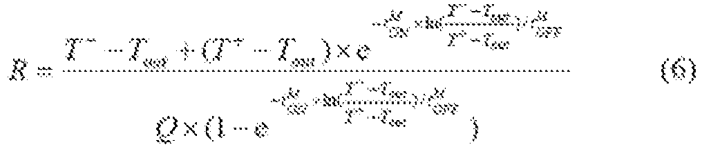

Step 5. For each set of R, C and Q obtained in Step 4, calculate if Equation (10) is satisfied, for T + = 72°F Tout ranges from min{T 0(i)} to max{T 0(i)} in M(i), i = 1,2, ... , NM. If not, this set of R, C and Q will be discarded. 
Step 6.For each remaining set of R, C and Q after Step 5, calculate if Equation (11) is satisfied. If not, this set of R, C and Q will be discarded.

Step 7.For each remaining set of R, C and Q after Step 6, select the set of R, C and Q which minimized Equation (13), where t̃ON (Tout ) and t̃OFF (Tout ) are calculated,


Step 8.Repeat Step 1 throughStep 7 for all houses. - As illustrated in
Figs. 7A and 7B , the estimation errors oft ON and tOFF have different trends. If one RfCfQf set is used for modeling both the ON and OFF cycles, a simple parameter adjustment is not feasible because when errors int ON are reduced, errors in tOFF will increase. From equations (8) and (9), tON is related with Rf, Cf, Qf but tOFF is only related with R×C. Therefore, a Decoupled-ETP model is used to separate the modeling of ON and OFF cycles. The RCQ parameters are made a function of Tout to reduce the modeling error corresponding to the Tout variations. Contrary to equations (1) and (2), in the Decoupled-ETP model, Troom and uac at t=k+ 1 are calculated as:

- When Tout is constant, equation (14) can be rewritten as:


- For the OFF cycle, define Rf ×Cf = fRC (Tout ) such that the RfCf value is a function of Tout. From equation (17),

Fig. 9A is a graph illustrating actual values and the linear correlation between Rf × Cf and Tout. Therefore, the linear regression model used to calculate fRC(Tout) is
- To avoid modeling temperature sensitivity of all three RCQ parameters, let R=Rf and C=Cf (obtained above) to derive the ON cycle RCQ parameter. When the values of R and C are fixed, Q is made a function of Tout, leading to

- The correlation between Q and Tout derived from the one hundred houses was calculated. The mean of correlation coefficient was 0.941 and the standard deviation was 0.048.
Fig. 9B is a graph illustrating linear correlation between Q and Tout. The linear regression model used to calculate Q for each Tout is
- After Q is calculated for each Tout using equation (21), the estimated ON cycle duration, t̂ON , can be calculated as

-
Fig. 10 is a flow chart ofAlgorithm 2 for a Decoupled-ETP model. The process steps ofAlgorithm 2 can be implemented on a power Decoupled-ETP model processor 140 or other similar processor having circuitry configured to implement the process steps ofAlgorithm 2. - In step S 1010, Rf , Cf , Qf , and HVAC power consumption and ambient temperature Tout of the ith house are input. Input parameters Rf , Cf , Qf , are calculated as described herein with reference to step S480 in
Fig. 4 . HVAC power consumption and ambient temperature Tout are obtained from theHVAC consumption database 120 for the ith house. - In step S1020, fRC(Tout) is calculated.

Fig. 4 -
Fig. 9A is a graph illustrating actual calculated results of fRC(Tout) for each Tout. - In step S1030, a linear fit is performed of fRC(Tout) for each Tout, an example of which is illustrated in
Fig. 9A . - In step S1040, Q(Tout) is calculated for each Tout based on:

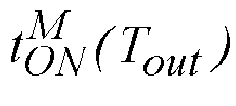
Fig. 4 . -
Fig. 9B is a graph illustrating actual calculated results of Q(Tout) for each Tout. - In step S 1050, a linear fit of Q(Tout ) is performed for each Tout, an example of which is illustrated in
Fig. 9B . - In step S 1060, a Decoupled-ETP model is built for the ith house.


- In step S 1065, it is determined whether an end of a list of houses has been reached. If the end of the house list has been reached (a "YES" decision in step S1065), the process ends. If the end of the house list has not been reached (a "NO" decision in step S1065) the process continues to step S 1070.
- In step S 1070, a counter increments to the (i + 1)th house and
Algorithm 2 returns to step S 1010 to repeat the process for the next house. - The following exemplary algorithm may be used for deriving the Decoupled-ETP model according to embodiments described herein.
-
Step 1.Input dataset of the i th (i=1, 2, ..., N house) house and repeat Step 1 throughStep 7 inAlgorithm 1.Step 2.For each remaining set of R, C and Q after Step 6 inAlgorithm 1, build Vector

Step 3.Calculate 
Step 4. Use linear regression fRC (Tout ) = kRC × Tout + bRC to fit the relation between f̃RC (i) and T 0(i), i = 1,2, ... , ND. Step 5. Calculate 
Step 6. Use linear regression fQ (Tout ) = kQ × Tout + bQ to fit the relation between f̃Q (i) and T 0(i), i = 1,2, ... , ND. Step 7. Build the Decoupled ETP model based on Equations (14)-(15). Step 8.Repeat Step 1 throughStep 7 for all datasets in each house. -
Fig. 11 is a bar graph illustrating a comparison between the estimated ON and OFF durations and the median of the actual ON/OFF durations with respect to outdoor temperature. Compared withFig. 8 for the ETP model, the accuracy of the prediction of the Decoupled-ETP model is significantly improved. The validation test for the one hundred houses was run using the PECAN street data set. The average errors between actual median of tON and tOFF and the estimated t̂ON and t̂OFF were calculated. The average error among the one hundred houses over the full range of Tout values was 4.02 and 2.05 minutes for the ETP model and the Decoupled-ETP model, respectively. If considering only the low (Tout <76°F) or the high (Tout >95°F) outdoor temperature cases, the modeling error of the Decoupled-ETP model is normally 10~20 minutes less than that of the ETP model. - The Decoupled-ETP model can be applied to model all TCAs as long as the consumptions are regulated by a consistent thermostat setting without being distorted by activities of occupants, such as opening the doors or windows for a prolonged period, frequently changing thermostat set points, or manually shutting down the TCA devices, etc. However, in practice, TCA operations during daytime can heavily be distorted by human activities, as illustrated in
Figs. 3A and 3C . For most houses, the most usable data for deriving TCA models are the data measured between midnight and early morning when the occupants are asleep, such that the influence of their activities is a minimum. However, for an HVAC unit, using only the midnight data can cause an inaccuracy since it does not account for the impact of solar radiations on the thermal dynamics of the house. - To address this issue, an Adjusted Decoupled-ETP model is used to tune the parameters of the Decoupled-ETP model, which was derived using only the midnight data. With the Adjusted Decoupled-ETP model, the day-time operation can also be accurately modeled.
- When the HVAC unit is ON, Troom at t=
k + 1 can be calculated as
- When the HVAC unit is OFF, Troom at t=
k + 1 can be calculated as

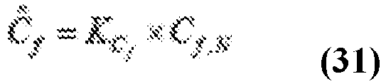


- In equations (28) and (29), Rf,N, Cf,N, fQ,N(Tout), and fRC,N(Tout) are the parameters of the Decoupled-ETP model calculated using the midnight data set. KR
f , KCf , KQ(Tout) and KRC(Tout) are the adjustment coefficients for modeling daytime HVAC cycling behaviors. - To derive these coefficients, n households with at least five days of 24-hour HVAC consumptions were selected, during which period there were no obvious distortions caused by occupants' activities. A NIGHT model and a WHOLE-DAY model represent the Decoupled-ETP model derived using the midnight data and the whole-day data, respectively. The NIGHT model parameters of the ilh HVAC unit include

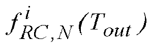


- The adjustment coefficients can be calculated as follows.


- To account for the saturation effect of the HVAC unit in low or high temperature ranges, a capped linear regression model is used.

-
Fig. 12A is a graph illustrating an example of
Fig. 12B is a graph illustrating the linear fit model K̃Q with respect to Tout. - KRC (Tout ) is calculated as


-
Fig. 13A is a graph illustrating an example of
Fig. 13B is a graph illustrating the second order polynomial model K̃Q versus Tout. - When the adjustment coefficients are derived, only the middle night data is used to derive the Decoupled-ETP model parameters. The NIGHT model parameters are adjusted using equations (28) and (29) so that when modeling the daytime HVAC cycling behaviors, the impact of solar radiation can be reflected appropriately.
-
Fig. 14 is a flow chart ofAlgorithm 3 for the Adjusted Decoupled-ETP model. The process steps ofAlgorithm 3 can be implemented on a power Adjusted Decoupled-ETP model processor 150 or other similar processor having circuitry configured to implement the process steps ofAlgorithm 3. - In step S1410, n non-distorted data is input. For example, data can cover a 5-day, 24-hour period for household HVAC power consumption and ambient temperature data from the
HVAC consumption database 120.Fig. 3B is a graph associated withStep 1 illustrating an acceptable HVAC consumption curve. - In step S1420, the midnight data is used to calculate the Decoupled-ETP model parameters for each household HVAC,

Fig. 10 ). - In step S1430, whole-day data is used to calculate the Decoupled-ETP model parameters for each household HVAC,

Fig. 10 ). - In step S 1440, adjustment coefficients KR
f , KCf , KQ(Tout) and KRC(Tout) are calculated based on:


- In step S 1450, a linear fit KQ(Tout) and a polynomial fit KRC(Tout) are performed.


- In step S 1460, an Adjusted Decoupled-ETP model is built for each HVAC unit.


- The following exemplary algorithm may be used for deriving the Adjusted Decoupled-ETP model according to embodiments described herein.
-
Step 1.Select at least Nadj houses data (Pac(t), T out(t)) under the same season and repeat Algorithm 1 to select at least NS single family houses, NA apartments and NT townhouses that are capable to derive both Nighttime and Whole-day HVAC models.Step 2.For each selected single family house i, repeat Algorithm 2Step 1 throughStep 7 to obtain the whole-day Decoupled-ETP model parameters
and the nighttime Decoupled-ETP model parameters 
Step 3. Calculate adjustment gain KR f ,S, KCf ,S, K̃Q,S (Tout ), K̃RC,S(Tout) modified for single family data, s.


Step 4. Use capped linear and quadratic regression in Equations (38) and (40) to fit the relation between K̃Q,S (Tout ), K̃RC,S (Tout ) and Tout . 

Step 5. Repeat Step 2 - Step 4 for selected NA apartments and obtain adjustment gain KR f ,A, KCf ,A, KQ,A (Tout ), KRC,A (Tout ). Repeat Step 2 - Step 4 for selected NT townhouses and obtain adjustment gain KRf ,T, KCf ,T, KQ,T (Tout ), KRC,T (Tout ).Step 6.For each house to model, repeat Step 1 - Step 7 inAlgorithm 2 and build the nighttime decoupled-ETP model with parameters
f , KCf , KQ (Tout ), KRC(Tout) obtained in Step 4 throughStep 5.Step 7.Build the Adjusted Decoupled-ETP model using the following. 




- Simulation results compared the performance of the ETP model with the Decoupled-ETP model and the Adjusted Decoupled-ETP model. Two performance criteria were used. The first criterion was the error in the measured and estimated total ON time durations and the second is the total number of switchings. The total ON duration reflects the accuracy of the model when estimating the total power consumptions. The total number of switchings indicates the accuracy of the model when estimating the switching behaviors.
- The accuracy of the ETP models and the Decoupled-ETP models were verified using House #3192 data and verification results using 100 HVAC units.
- Table III shows the results comparing the errors in the total ON time and the total number of switchings when using the ETP model and the Decoupled-ETP model, respectively. APE is defined as the absolute percentage error.

Table III. Performance Comparison Total ON Time Total Switchings House #3192 Time (min) APE # times APE Actual 6788 NA 751 NA ETP Model 6471 4.66% 702 6.52% Decoupled ETP 6784 0.01% 766 2.00% -
Figs. 15A and 15B are bar graphs illustrating a mean absolute percentage error (MAPE) and a standard deviation (SD) of the total ON time based on night time data of one hundred HVAC units. The error distribution is for the ETP or the Decoupled-ETP model based on midnight data.Figs. 15C and 15D are bar graphs illustrating MAPE and a SD of the total number of switchings of one hundred HVAC units. Table IV also illustrates these results. The results illustrate the total ON time and the total number of switchings of the Decoupled-ETP model have a much lower MAPE and SD than those of the ETP model. The error distribution for the ETP model for ON time APE illustrated inFig. 15A also confirms that the Decoupled-ETP model for ON time APE illustrated inFig. 15B performs significantly better than the ETP model and its performance is consistent across the households.Table IV. Performance Comparison Using 100 Houses Data Total ON Time Total Switching Times 100 Houses MAPE SD MAPE SD ETP Model 14.52% 10.55% 12.69% 12.56% Decoupled ETP 4.23% 3.35% 3.49% 2.95% - The performance of the ETP model, the Decoupled-ETP model, and the Adjusted Decoupled-ETP model was verified using 24-hour whole day data, as illustrated below. The performance of the Adjusted Decoupled-ETP models was verified using House #3456 data and verification results using 50 HVAC units.
- Table V illustrates the comparison of errors in the total ON time and the number of switchings for different models.
Table V. Results Comparison, House #3456 at Austin, Texas from 15:18 pm July 12 th to 21:57 pm August 2 nd . 2015 Total ON Time Total Switchings House #3456 Data Input Time (min) APE # Times APE Actual NA 5779 NA 669 NA ETP1 Midnight 11713 102.68% 946 41.30% ETP2 Whole day 5487 5.05% 583 12.86% Decoupled- ETP 1Midnight 6338 9.68% 733 9.62% Decoupled-ETP2 Whole day 5765 0.25% 335 0.10% Adjusted Decoupled-ETP Midnight 6152 6.46% 708 5.77% - Column "Data Input" refers to the type of data that was used to build the model. The Whole-day data used the 24-hr consumption of the HVAC unit in house #3456 as inputs and the Night data used 12 a.m. to 5 am. HVAC consumption as inputs. The Decoupled-ETP model using the whole-day data as inputs had the best performance with the lowest errors. When the midnight model was used without being adjusted, the modeling error increased sharply. When using the Adjusted Decoupled-ETP model, the error was reduced by close to 50%. The error was defined as the cumulated error of 21 days, the average daily modeling errors in the total ON time were within 18 minutes and the average errors in modeling the number of switches were within two times. This illustrates an improved performance when modeling the HVAC switching characteristics
- Table VI and
Figs. 16A through 16F verify theCase 1 results using data collected from fifty houses during summer months.Figs. 16A and 16B are bar graphs illustrating ON time APE and Switching APE, respectively for the Decoupled-ETP1 model.Figs. 16C and16D are bar graphs illustrating ON time APE and Switching APE, respectively for the Decoupled-ETP2 model.Figs. 16E and 16F are bar graphs illustrating ON time APE and Switching APE, respectively for the Adjusted Decoupled-ETP model. The results show that all three Decoupled-ETP model performances were consistent across households. If only the midnight data is usable, the Adjusted Decoupled-ETP model can be used for modeling the day-time HVAC behaviors.Table VI. Performance Comparison Using 50 Houses Data Total ON Time Total Switchings 50 Houses Data Input MAPE SD MAPE SD ETP1 Midnight 85.72% 38.96% 46.69% 15.70% ETP2 Whole day 9.16% 7.44% 8.61% 7.61% Decoupled- ETP 1Midnight 17.84% 14.73% 13.07% 12.77% Decoupled-ETP2 Whole day 2.31% 1.79% 3.00% 1.81% Adjusted Decoupled-ETP Midnight 8.86% 7.09% 7.92% 6.33% - Previous systems and methods have attempted to reduce peak power by controlling generators, thermostats, etc. based on a centralized system model, architecture, or configuration. Some systems and methods have modeled uncertainties in aggregated HVAC loads using a state queueing model, wherein no control is involved. Other methods reshape the energy demand profile of aggregated buildings, which is also based on a centralized system design and model. One HVAC aggregated model is based on an ETP model and a centralized control strategy. Other systems and methods use an HVAC load control strategy to follow the targeted load curve, which is based on a centralized multi-objective system model, architecture, or configuration. Still other systems and methods use a state space-based HVAC simulation model based on an ETP model, wherein no control is involved.
- In contrast, embodiments herein describe data-driven methods and models to estimate the ETP model parameters of TCAs using their power consumptions and ambient temperature data as inputs. The modeling of HVAC units is used to decouple the modeling of the ON and OFF cycles, which simplifies the derivation of modeling parameters and significantly improves the modeling accuracy. To adjust the distortion of human activities on HVAC cycling behaviors, midnight data is used for ETP model parameter estimation. A tuning process is used to adjust the nighttime models due to the impact of solar radiation.
- In one implementation, the functions and processes of the
modeling system 100 can be implemented in part by acomputer 1700 illustrated inFig. 17 . In particular,power consumption database 120, powerETP model processor 130, power Decoupled-ETP model processor 140, power Adjusted Decoupled-ETP model processor 150, and/orprediction processor 160 con be implemented by thecomputer 1700, either separately or together as one or more units. - A hardware description of the
computer 1700 according to exemplary embodiments is described with reference toFig. 17 . InFig. 17 , thecomputer 1700 includes aCPU 1701 which performs the processes described herein. The process data and instructions may be stored inmemory 1702. These processes and instructions may also be stored on astorage medium disk 1704 such as a hard drive (HDD) or portable storage medium or may be stored remotely. Further, the claimed advancements are not limited by the form of the computer-readable media on which the instructions of the inventive process are stored. For example, the instructions may be stored on CDs, DVDs, in FLASH memory, RAM, ROM, PROM, EPROM, EEPROM, hard disk or any other information processing device with which thecomputer 1700 communicates, such as a server or computer. - Further, the claimed advancements may be provided as a utility application, background daemon, or component of an operating system, or combination thereof, executing in conjunction with
CPU 1701 and an operating system such as Microsoft® Windows®, UNIX®, Oracle ® Solaris, LINUX®, Apple macOS® and other systems known to those skilled in the art. - In order to achieve the
computer 1700, the hardware elements may be realized by various circuitry elements, known to those skilled in the art. For example,CPU 1701 may be a Xenon® or Core® processor from Intel Corporation of America or an Opteron® processor from AMD of America, or may be other processor types that would be recognized by one of ordinary skill in the art. Alternatively, theCPU 1701 may be implemented on an FPGA, ASIC, PLD or using discrete logic circuits, as one of ordinary skill in the art would recognize Further,CPU 1701 may be implemented as multiple processors cooperatively working in parallel to perform the instructions of the inventive processes described above. - The
computer 1700 inFig. 17 also includes anetwork controller 1706, such as an Intel Ethernet PRO network interface card from Intel Corporation of America, for interfacing withnetwork 1724. As can be appreciated, thenetwork 1724 can be a public network, such as the Internet, or a private network such as LAN or WAN network, or any combination thereof and can also include PSTN or ISDN sub-networks. Thenetwork 1724 can also be wired, such as an Ethernet network, or can be wireless such as a cellular network including EDGE, 3G and 4G wireless cellular systems. The wireless network can also be WiFi®, Bluetooth®, or any other wireless form of communication that is known. - The
computer 1700 further includes adisplay controller 1708, such as a NVIDIA® GeForce® GTX or Quadro® graphics adaptor from NVIDIA Corporation of America for interfacing withdisplay 1710, such as a Hewlett Packard® HPL2445w LCD monitor. A general purpose I/O interface 1712 interfaces with a keyboard and/ormouse 1714 as well as an optionaltouch screen panel 1716 on or separate fromdisplay 1710. General purpose I/O interface 1712 also connects to a variety ofperipherals 1718 including printers and scanners, such as an OfficeJet® or DeskJet® from Hewlett Packard. - The general
purpose storage controller 1720 connects thestorage medium disk 1704 withcommunication bus 1722, which may be an ISA, EISA, VESA, PCI, or similar, for interconnecting all of the components of thecomputer 1700. A description of the general features and functionality of thedisplay 1710, keyboard and/ormouse 1714, as well as thedisplay controller 1708,storage controller 1720,network controller 1706, and general purpose I/O interface 1712 is omitted herein for brevity as these features are known. - A number of implementations have been described. Nevertheless, it will be understood that various modifications may be made. For example, preferable results may be achieved if the steps of the disclosed techniques were performed in a different sequence, if components in the disclosed systems were combined in a different manner, or if the components were replaced or supplemented by other components. The functions, processes, and algorithms described herein may be performed in hardware or software executed by hardware, including computer processors and/or programmable circuits configured to execute program code and/or computer instructions to execute the functions, processes, and algorithms described herein. Additionally, an implementation may be performed on modules or hardware not identical to those described.
Claims (13)
- A method of improving an energy parameter estimation, comprising:storing power consumption data retrieved from a plurality of power systems into a power consumption database;converting, via processing circuitry, the power consumption data into power activated time cycles and power non-activated time cycles;calculating, via the processing circuitry, median time values of the power activated time cycles and the power non-activated time cycles for respective outdoor temperatures;deriving a thermal resistance (R) parameter and a capacitance (C) parameter for a predetermined heat flow (Q) parameter at each of the respective outdoor temperatures for the plurality of power systems;comparing, via the processing circuitry, the converted power activated time cycles to the actual power activated time cycles for the plurality of power systems to determine if the converted power activated time cycles match within a predefined margin of error the actual power activated time cycles;comparing, via the processing circuitry, the converted power non-activated time cycles to the actual power non-activated time cycles for the plurality of power systems to determine if the converted power non-activated time cycles match within a predefined margin of error the actual power non-activated time cycles;calculating a first improved resistance-capacitance-heat flow (RCQ) parameter set and a respective first outdoor temperature for the compared and converted power activated time cycles to the actual power activated time cycles;calculating a second improved RCQ parameter set and a respective second outdoor temperature for the compared and converted power non-activated time cycles to the actual power non-activated time cycles; andimproving the energy parameter estimation by executing the first and second improved RCQ parameter sets at the respective first and second outside temperatures for each of the plurality of power systems , wherein the improving the energy parameter estimation identifies energy efficiencies to reduce a total energy load within said each of the plurality of power systems.
- The method of claim 1, wherein the improved RCQ parameter set is determined by minimizing an error between the converted power activated time cycles and the actual power activated time cycles, and between the converted power non-activated time cycles and the actual power non-activated time cycles.
- The method of claim 1, wherein the power consumption data is limited to data within a temperature range between a predefined upper limit temperature and a predefined lower limit temperature.
- The method of claim 1, wherein the method comprises an equivalent thermal parameter (ETP) model for improving the energy parameter estimation.
- The method of claim 1, further comprising:calculating the Q parameter at each of the respective outdoor temperatures during the power activated time cycles for the plurality of power systems; andcalculating the R parameter and the C parameter at each of the respective outdoor temperatures during the power non-activated time cycles for the plurality of power systems.
- The method of claim 5, further comprising:calculating, via the processing circuitry, an estimated duration of each of the power activated time cycles from the Q parameter calculated at each of the respective outdoor temperatures;calculating, via the processing circuitry, an estimated duration of each of the power non-activated time cycles from the R parameter and the C parameter calculated at each of the respective outdoor temperatures; andimproving the energy parameter estimation to reduce errors corresponding to variations in said each of the respective outdoor temperatures by decoupling daytime parameters from night time parameters via the estimated duration of said each of the power activated time cycles from the Q parameter and via the estimated duration of said each of the power non-activated time cycles from the R parameter and the C parameter.
- The method of claim 1, further comprising:calculating an R adjustment coefficient as a ratio of a whole-day R parameter to a night-time R parameter;calculating a C adjustment coefficient as a ratio of a whole-day C parameter to a night-time C parameter;calculating a Q adjustment coefficient at said each of the respective outdoor temperatures as a ratio of a whole-day Q parameter to a night-time Q parameter at said each of the respective outdoor temperatures; andcalculating an RC adjustment coefficient at said each of the respective outdoor temperatures as a ratio of a whole-day RC parameter to a night-time RC parameter at said each of the respective outdoor temperatures, wherein the whole-day R parameter, the whole-day C parameter, the whole-day Q parameter, and the whole-day RC parameter are calculated from data taken over a 24-hour period of time, andwherein the night-time R parameter, the night-time C parameter, the night-time Q parameter, and the night-time RC parameter are calculated from data taken during an absence of solar exposure.
- The method of claim 7, further comprising:calculating a daytime R parameter as a product of the R adjustment coefficient and a night-time optimum R parameter;calculating a daytime C parameter as a product of the C adjustment coefficient and a night-time optimum C parameter;calculating a daytime Q parameter as a product of the Q adjustment coefficient and a night-time optimum Q parameter at said each of the respective outdoor temperatures;calculating a daytime RC parameter as a product of the RC adjustment coefficient and a night-time optimum RC parameter at said each of the respective outdoor temperatures; andimproving the energy parameter estimation to reduce errors corresponding to variations in solar exposure by adjusting night time parameters to be used as daytime parameters via the daytime R parameter, the daytime C parameter, the daytime Q parameter, and the daytime RC parameter.
- The method of claim 1, wherein the plurality of power systems includes a plurality of thermostatically controlled appliances (TCAs).
- A decoupled equivalent thermal parameter (ETP) model processor, comprising:
circuitry configured tostore power consumption data retrieved from a plurality of power systems into a power consumption database;convert the power consumption data into power activated time cycles and power non-activated time cycles;calculate median time values of the power activated time cycles and the power non-activated time cycles for respective outdoor temperatures;derive parameters for a thermal resistance (R) parameter and a capacitance (C) parameter for a predetermined heat flow (Q) parameter at each of the respective outdoor temperatures for the plurality of power systems;compare the converted power activated time cycles to the actual power activated time cycles for the plurality of power systems;compare the converted power non-activated time cycles to the actual power non-activated time cycles for the plurality of power systems;calculate a first improved resistance-capacitance-heat flow (RCQ) parameter set and a respective first outdoor temperature for the compared and converted power activated time cycles to the actual power activated time cycles;calculate a second improved RCQ parameter set and a respective second outdoor temperature for the compared and converted power non-activated time cycles to the actual power non-activated time cycles;calculate the Q parameter at each of the respective outdoor temperatures during the power activated time cycles for the plurality of power systems; andcalculate the R parameter and the C parameter at each of the respective outdoor temperatures during the power non-activated time cycles for the plurality of power systems. - The decoupled ETP model processor of claim 10, wherein the circuitry is further configured to:calculate an estimated duration of each of the power activated time cycles from the Q parameter calculated at each of the respective outdoor temperatures; andcalculate an estimated duration of each of the power non-activated time cycles from the R parameter and the C parameter calculated at each of the respective outdoor temperatures,wherein the calculated Q parameter, the calculated R parameter, and the calculated C parameter improve energy parameter estimation to reduce errors corresponding to variations in said each of the respective outdoor temperatures by decoupling daytime parameters from night time parameters via the estimated duration of said each of the power activated time cycles from the Q parameter and via the estimated duration of said each of the power non-activated time cycles from the R parameter and the C parameter.
- The decoupled ETP model processor of claim 10, wherein the improved RCQ parameter set is determined by minimizing an error between the converted power activated time cycles and the actual power activated time cycles, and between the converted power non-activated time cycles and the actual power non-activated time cycles.
- The decoupled ETP model processor of claim 10, wherein the plurality of power systems includes a plurality of thermostatically controlled appliances (TCAs).
Applications Claiming Priority (1)
| Application Number | Priority Date | Filing Date | Title |
|---|---|---|---|
| PCT/US2017/055743 WO2019074475A1 (en) | 2017-10-09 | 2017-10-09 | Decoupled modeling methods and systems |
Publications (2)
| Publication Number | Publication Date |
|---|---|
| EP3695288A1 EP3695288A1 (en) | 2020-08-19 |
| EP3695288B1 true EP3695288B1 (en) | 2023-07-19 |
Family
ID=60262991
Family Applications (1)
| Application Number | Title | Priority Date | Filing Date |
|---|---|---|---|
| EP17794455.0A Active EP3695288B1 (en) | 2017-10-09 | 2017-10-09 | Decoupled modeling methods and systems |
Country Status (6)
| Country | Link |
|---|---|
| US (1) | US11514537B2 (en) |
| EP (1) | EP3695288B1 (en) |
| CN (1) | CN111542796B (en) |
| AU (1) | AU2017435881B2 (en) |
| ES (1) | ES2959791T3 (en) |
| WO (1) | WO2019074475A1 (en) |
Families Citing this family (5)
| Publication number | Priority date | Publication date | Assignee | Title |
|---|---|---|---|---|
| CN113028604A (en) * | 2020-12-04 | 2021-06-25 | 国家电网有限公司 | Temperature regulation control and scheduling method based on aggregated air conditioner |
| CN113219930A (en) * | 2021-05-21 | 2021-08-06 | 上海交通大学 | Variable frequency air conditioner second-order equivalent thermal parameter model online identification method based on particle swarm optimization |
| CN115755657B (en) * | 2021-09-03 | 2024-07-30 | 北京机械设备研究所 | Near peak staggering control method based on vehicle-mounted system |
| CN114738958B (en) * | 2022-04-06 | 2024-01-19 | 合肥工业大学 | Variable frequency air conditioning load optimization control method and system |
| CN119778837B (en) * | 2024-12-16 | 2026-07-21 | 广东电网有限责任公司 | Method and device for determining air conditioner load polymer regulation parameters and electronic equipment |
Family Cites Families (27)
| Publication number | Priority date | Publication date | Assignee | Title |
|---|---|---|---|---|
| US4123792A (en) * | 1977-04-07 | 1978-10-31 | Gephart Don A | Circuit for monitoring the mechanical power from an induction motor and for detecting excessive heat exchanger icing |
| US7155353B2 (en) * | 2002-04-25 | 2006-12-26 | Daicel Chemical Industries, Ltd. | Method for determining charging capacitance of capacitor |
| US7132960B2 (en) * | 2002-10-15 | 2006-11-07 | Honeywell International Inc. | Approach monitoring and advisory system and method |
| US7089129B2 (en) * | 2003-11-12 | 2006-08-08 | International Business Machines Corporation | Electromigration check of signal nets using net capacitance to evaluate thermal characteristics |
| WO2006028110A1 (en) * | 2004-09-07 | 2006-03-16 | Chugai Seiyaku Kabushiki Kaisha | Process for producing water-soluble hyaluronic acid modification |
| JP4514669B2 (en) * | 2005-07-29 | 2010-07-28 | エヌイーシー ショット コンポーネンツ株式会社 | Protection device using thermal fuse |
| US8957790B2 (en) * | 2009-01-06 | 2015-02-17 | The Boeing Company | System and method for cruise monitoring and alerting |
| US8355827B2 (en) * | 2010-04-08 | 2013-01-15 | Energy Resource Management Corp | Energy-saving measurement, adjustment and monetization system and method |
| CN102162660B (en) * | 2011-06-10 | 2013-01-02 | 山东高唐融博新能源开发有限公司 | Natural-dehumidifying air-refrigerating air conditioner |
| US9362749B2 (en) * | 2012-04-20 | 2016-06-07 | Battelle Memorial Institute | Controller for thermostatically controlled loads |
| US9459634B2 (en) * | 2013-02-08 | 2016-10-04 | Trane International Inc. | HVAC system with improved control switching |
| JP2015004498A (en) * | 2013-06-24 | 2015-01-08 | 東芝キヤリア株式会社 | Heat source equipment |
| CN103389749B (en) * | 2013-07-01 | 2015-12-23 | 浙江大学 | A kind of temperature control system |
| CN103472088B (en) * | 2013-08-13 | 2015-07-08 | 杭州远方光电信息股份有限公司 | Thermal resistance analysis method |
| US10230240B2 (en) | 2013-10-22 | 2019-03-12 | University Of Florida Research Foundation, Incorporated | Low-frequency ancillary power grid services |
| CN103561499A (en) * | 2013-10-23 | 2014-02-05 | 浙江耀恒光电科技有限公司 | Low power consumption stand-by circuit of tandem type LED circuit |
| US9817375B2 (en) | 2014-02-26 | 2017-11-14 | Board Of Trustees Of The University Of Alabama | Systems and methods for modeling energy consumption and creating demand response strategies using learning-based approaches |
| US9817409B2 (en) | 2014-05-27 | 2017-11-14 | Nishihara Energy, Inc. | Method and apparatus for distributed control of thermostatic electric loads using high-granularity energy usage data |
| CN104214912B (en) * | 2014-09-24 | 2017-02-15 | 东南大学 | Aggregation air conditioning load scheduling method based on temperature set value adjustment |
| KR101598979B1 (en) * | 2014-10-07 | 2016-03-02 | 주식회사 인코어드 테크놀로지스 | Method and apparatus for estimating power consumption based on temperature |
| CN104566868B (en) * | 2015-01-27 | 2017-09-08 | 杭州宏成节能科技有限公司 | A kind of central air conditioning system and its control method |
| CN104896660B (en) * | 2015-05-20 | 2017-09-08 | 中南大学 | A kind of office building room conditioning temperature optimization establishing method |
| CN105116942B (en) * | 2015-06-26 | 2017-03-15 | 国网山西省电力公司 | A kind of thermostatic control intelligence load combined optimization method |
| CN105020859B (en) * | 2015-08-04 | 2017-11-17 | 深圳供电局有限公司 | A central air-conditioning load reduction and temperature adjustment method based on the principle of equal comfort loss |
| CN105042800B (en) * | 2015-09-01 | 2017-11-07 | 东南大学 | Convertible frequency air-conditioner load modeling and progress control method based on demand response |
| CN105352108B (en) * | 2015-09-29 | 2019-03-08 | 中国电力科学研究院 | A load optimization control method based on air-conditioning power consumption mode |
| CN105627506A (en) * | 2015-12-25 | 2016-06-01 | 深圳达实智能股份有限公司 | Building cooling load prediction method and device of air conditioning refrigerator |
-
2017
- 2017-10-09 AU AU2017435881A patent/AU2017435881B2/en not_active Ceased
- 2017-10-09 US US16/754,267 patent/US11514537B2/en active Active
- 2017-10-09 WO PCT/US2017/055743 patent/WO2019074475A1/en not_active Ceased
- 2017-10-09 EP EP17794455.0A patent/EP3695288B1/en active Active
- 2017-10-09 CN CN201780096382.4A patent/CN111542796B/en active Active
- 2017-10-09 ES ES17794455T patent/ES2959791T3/en active Active
Also Published As
| Publication number | Publication date |
|---|---|
| EP3695288A1 (en) | 2020-08-19 |
| US11514537B2 (en) | 2022-11-29 |
| CN111542796A (en) | 2020-08-14 |
| AU2017435881A1 (en) | 2020-04-09 |
| ES2959791T3 (en) | 2024-02-28 |
| US20200302561A1 (en) | 2020-09-24 |
| WO2019074475A1 (en) | 2019-04-18 |
| AU2017435881B2 (en) | 2023-07-27 |
| CN111542796B (en) | 2021-12-10 |
Similar Documents
| Publication | Publication Date | Title |
|---|---|---|
| US20230281360A1 (en) | System and method balance-point-thermal-conductivity-based building analysis the aid of a digital computer | |
| US11514537B2 (en) | Decoupled modeling methods and systems | |
| JP5572799B2 (en) | Air conditioning system controller | |
| US11859838B2 (en) | System and method for aligning HVAC consumption with renewable power production with the aid of a digital computer | |
| Dong et al. | An investigation on energy-related occupancy behavior for low-income residential buildings | |
| US9348392B2 (en) | Systems and methods for measuring and verifying energy savings in buildings | |
| Acosta et al. | Energy savings and guaranteed thermal comfort in hotel rooms through nonlinear model predictive controllers | |
| Zhou et al. | Quantitative comparison of data-driven and physics-based models for commercial building HVAC systems | |
| Touretzky et al. | Building-level power demand forecasting framework using building specific inputs: Development and applications | |
| Sonnekalb et al. | Smart hot water control with learned human behavior for minimal energy consumption | |
| CN107120794A (en) | Air conditioner operating condition adjusting method and air conditioner | |
| Chen et al. | Inverse energy model development via high-dimensional data analysis and sub-metering priority in building data monitoring | |
| JP6384791B2 (en) | Thermal insulation performance estimation device, program | |
| US20210192469A1 (en) | Building control system with peer analysis for predictive models | |
| US20200278130A1 (en) | Operation control method, storage medium, and operation control device | |
| US20190311283A1 (en) | System And Method For Estimating Periodic Fuel Consumption for Cooling Of a Building With the Aid Of a Digital Computer | |
| US10503192B2 (en) | Energy consumption modeling | |
| WO2017151113A1 (en) | Estimating the impact of weather in electricity bills | |
| WO2016051477A1 (en) | Service system and method for assisting improvement of air-conditioning of building | |
| He et al. | Optimal Energy Consumption Prediction for University Buildings Based on Energy Classification Using GA-BP | |
| Johnson Jr | Improved Electric Load Modeling of Residential Air Conditioning | |
| Hilliard et al. | A tool for evaluating the performance of simplified models for predictive control applications | |
| Ozoh et al. | A procedure for the analysis of multivariate factors affecting electricity consumption | |
| Ota et al. | Energy efficient residential thermal control with wireless sensor networks: A case study for air conditioning in California | |
| Alamos et al. | Asset Optimization through demand control |
Legal Events
| Date | Code | Title | Description |
|---|---|---|---|
| STAA | Information on the status of an ep patent application or granted ep patent |
Free format text: STATUS: UNKNOWN |
|
| STAA | Information on the status of an ep patent application or granted ep patent |
Free format text: STATUS: THE INTERNATIONAL PUBLICATION HAS BEEN MADE |
|
| PUAI | Public reference made under article 153(3) epc to a published international application that has entered the european phase |
Free format text: ORIGINAL CODE: 0009012 |
|
| STAA | Information on the status of an ep patent application or granted ep patent |
Free format text: STATUS: REQUEST FOR EXAMINATION WAS MADE |
|
| 17P | Request for examination filed |
Effective date: 20200401 |
|
| AK | Designated contracting states |
Kind code of ref document: A1 Designated state(s): AL AT BE BG CH CY CZ DE DK EE ES FI FR GB GR HR HU IE IS IT LI LT LU LV MC MK MT NL NO PL PT RO RS SE SI SK SM TR |
|
| AX | Request for extension of the european patent |
Extension state: BA ME |
|
| RIN1 | Information on inventor provided before grant (corrected) |
Inventor name: LU, JIAN Inventor name: ZENG, WENTE Inventor name: WANG, JIYU Inventor name: LU, NING |
|
| DAV | Request for validation of the european patent (deleted) | ||
| DAX | Request for extension of the european patent (deleted) | ||
| STAA | Information on the status of an ep patent application or granted ep patent |
Free format text: STATUS: EXAMINATION IS IN PROGRESS |
|
| 17Q | First examination report despatched |
Effective date: 20211125 |
|
| REG | Reference to a national code |
Ref country code: DE Ref legal event code: R079 Free format text: PREVIOUS MAIN CLASS: G05D0023190000 Ipc: G06Q0010040000 Ref document number: 602017071527 Country of ref document: DE |
|
| GRAP | Despatch of communication of intention to grant a patent |
Free format text: ORIGINAL CODE: EPIDOSNIGR1 |
|
| STAA | Information on the status of an ep patent application or granted ep patent |
Free format text: STATUS: GRANT OF PATENT IS INTENDED |
|
| RIC1 | Information provided on ipc code assigned before grant |
Ipc: F24F 140/60 20180101ALI20230113BHEP Ipc: F24F 11/63 20180101ALI20230113BHEP Ipc: F24F 11/46 20180101ALI20230113BHEP Ipc: G06Q 50/06 20120101ALI20230113BHEP Ipc: G06Q 10/04 20120101AFI20230113BHEP |
|
| INTG | Intention to grant announced |
Effective date: 20230207 |
|
| GRAS | Grant fee paid |
Free format text: ORIGINAL CODE: EPIDOSNIGR3 |
|
| GRAA | (expected) grant |
Free format text: ORIGINAL CODE: 0009210 |
|
| STAA | Information on the status of an ep patent application or granted ep patent |
Free format text: STATUS: THE PATENT HAS BEEN GRANTED |
|
| AK | Designated contracting states |
Kind code of ref document: B1 Designated state(s): AL AT BE BG CH CY CZ DE DK EE ES FI FR GB GR HR HU IE IS IT LI LT LU LV MC MK MT NL NO PL PT RO RS SE SI SK SM TR |
|
| REG | Reference to a national code |
Ref country code: GB Ref legal event code: FG4D |
|
| REG | Reference to a national code |
Ref country code: CH Ref legal event code: EP |
|
| REG | Reference to a national code |
Ref country code: DE Ref legal event code: R096 Ref document number: 602017071527 Country of ref document: DE |
|
| REG | Reference to a national code |
Ref country code: IE Ref legal event code: FG4D |
|
| REG | Reference to a national code |
Ref country code: LT Ref legal event code: MG9D |
|
| REG | Reference to a national code |
Ref country code: NL Ref legal event code: MP Effective date: 20230719 |
|
| REG | Reference to a national code |
Ref country code: AT Ref legal event code: MK05 Ref document number: 1590216 Country of ref document: AT Kind code of ref document: T Effective date: 20230719 |
|
| PG25 | Lapsed in a contracting state [announced via postgrant information from national office to epo] |
Ref country code: NL Free format text: LAPSE BECAUSE OF FAILURE TO SUBMIT A TRANSLATION OF THE DESCRIPTION OR TO PAY THE FEE WITHIN THE PRESCRIBED TIME-LIMIT Effective date: 20230719 |
|
| PG25 | Lapsed in a contracting state [announced via postgrant information from national office to epo] |
Ref country code: GR Free format text: LAPSE BECAUSE OF FAILURE TO SUBMIT A TRANSLATION OF THE DESCRIPTION OR TO PAY THE FEE WITHIN THE PRESCRIBED TIME-LIMIT Effective date: 20231020 |
|
| PG25 | Lapsed in a contracting state [announced via postgrant information from national office to epo] |
Ref country code: IS Free format text: LAPSE BECAUSE OF FAILURE TO SUBMIT A TRANSLATION OF THE DESCRIPTION OR TO PAY THE FEE WITHIN THE PRESCRIBED TIME-LIMIT Effective date: 20231119 |
|
| PG25 | Lapsed in a contracting state [announced via postgrant information from national office to epo] |
Ref country code: SE Free format text: LAPSE BECAUSE OF FAILURE TO SUBMIT A TRANSLATION OF THE DESCRIPTION OR TO PAY THE FEE WITHIN THE PRESCRIBED TIME-LIMIT Effective date: 20230719 Ref country code: RS Free format text: LAPSE BECAUSE OF FAILURE TO SUBMIT A TRANSLATION OF THE DESCRIPTION OR TO PAY THE FEE WITHIN THE PRESCRIBED TIME-LIMIT Effective date: 20230719 Ref country code: PT Free format text: LAPSE BECAUSE OF FAILURE TO SUBMIT A TRANSLATION OF THE DESCRIPTION OR TO PAY THE FEE WITHIN THE PRESCRIBED TIME-LIMIT Effective date: 20231120 Ref country code: NO Free format text: LAPSE BECAUSE OF FAILURE TO SUBMIT A TRANSLATION OF THE DESCRIPTION OR TO PAY THE FEE WITHIN THE PRESCRIBED TIME-LIMIT Effective date: 20231019 Ref country code: LV Free format text: LAPSE BECAUSE OF FAILURE TO SUBMIT A TRANSLATION OF THE DESCRIPTION OR TO PAY THE FEE WITHIN THE PRESCRIBED TIME-LIMIT Effective date: 20230719 Ref country code: LT Free format text: LAPSE BECAUSE OF FAILURE TO SUBMIT A TRANSLATION OF THE DESCRIPTION OR TO PAY THE FEE WITHIN THE PRESCRIBED TIME-LIMIT Effective date: 20230719 Ref country code: IS Free format text: LAPSE BECAUSE OF FAILURE TO SUBMIT A TRANSLATION OF THE DESCRIPTION OR TO PAY THE FEE WITHIN THE PRESCRIBED TIME-LIMIT Effective date: 20231119 Ref country code: HR Free format text: LAPSE BECAUSE OF FAILURE TO SUBMIT A TRANSLATION OF THE DESCRIPTION OR TO PAY THE FEE WITHIN THE PRESCRIBED TIME-LIMIT Effective date: 20230719 Ref country code: GR Free format text: LAPSE BECAUSE OF FAILURE TO SUBMIT A TRANSLATION OF THE DESCRIPTION OR TO PAY THE FEE WITHIN THE PRESCRIBED TIME-LIMIT Effective date: 20231020 Ref country code: FI Free format text: LAPSE BECAUSE OF FAILURE TO SUBMIT A TRANSLATION OF THE DESCRIPTION OR TO PAY THE FEE WITHIN THE PRESCRIBED TIME-LIMIT Effective date: 20230719 Ref country code: AT Free format text: LAPSE BECAUSE OF FAILURE TO SUBMIT A TRANSLATION OF THE DESCRIPTION OR TO PAY THE FEE WITHIN THE PRESCRIBED TIME-LIMIT Effective date: 20230719 |
|
| REG | Reference to a national code |
Ref country code: ES Ref legal event code: FG2A Ref document number: 2959791 Country of ref document: ES Kind code of ref document: T3 Effective date: 20240228 |
|
| PG25 | Lapsed in a contracting state [announced via postgrant information from national office to epo] |
Ref country code: PL Free format text: LAPSE BECAUSE OF FAILURE TO SUBMIT A TRANSLATION OF THE DESCRIPTION OR TO PAY THE FEE WITHIN THE PRESCRIBED TIME-LIMIT Effective date: 20230719 |
|
| REG | Reference to a national code |
Ref country code: DE Ref legal event code: R097 Ref document number: 602017071527 Country of ref document: DE |
|
| PG25 | Lapsed in a contracting state [announced via postgrant information from national office to epo] |
Ref country code: SM Free format text: LAPSE BECAUSE OF FAILURE TO SUBMIT A TRANSLATION OF THE DESCRIPTION OR TO PAY THE FEE WITHIN THE PRESCRIBED TIME-LIMIT Effective date: 20230719 Ref country code: RO Free format text: LAPSE BECAUSE OF FAILURE TO SUBMIT A TRANSLATION OF THE DESCRIPTION OR TO PAY THE FEE WITHIN THE PRESCRIBED TIME-LIMIT Effective date: 20230719 Ref country code: EE Free format text: LAPSE BECAUSE OF FAILURE TO SUBMIT A TRANSLATION OF THE DESCRIPTION OR TO PAY THE FEE WITHIN THE PRESCRIBED TIME-LIMIT Effective date: 20230719 Ref country code: DK Free format text: LAPSE BECAUSE OF FAILURE TO SUBMIT A TRANSLATION OF THE DESCRIPTION OR TO PAY THE FEE WITHIN THE PRESCRIBED TIME-LIMIT Effective date: 20230719 Ref country code: CZ Free format text: LAPSE BECAUSE OF FAILURE TO SUBMIT A TRANSLATION OF THE DESCRIPTION OR TO PAY THE FEE WITHIN THE PRESCRIBED TIME-LIMIT Effective date: 20230719 Ref country code: SK Free format text: LAPSE BECAUSE OF FAILURE TO SUBMIT A TRANSLATION OF THE DESCRIPTION OR TO PAY THE FEE WITHIN THE PRESCRIBED TIME-LIMIT Effective date: 20230719 |
|
| REG | Reference to a national code |
Ref country code: DE Ref legal event code: R119 Ref document number: 602017071527 Country of ref document: DE |
|
| PLBE | No opposition filed within time limit |
Free format text: ORIGINAL CODE: 0009261 |
|
| STAA | Information on the status of an ep patent application or granted ep patent |
Free format text: STATUS: NO OPPOSITION FILED WITHIN TIME LIMIT |
|
| PG25 | Lapsed in a contracting state [announced via postgrant information from national office to epo] |
Ref country code: IT Free format text: LAPSE BECAUSE OF FAILURE TO SUBMIT A TRANSLATION OF THE DESCRIPTION OR TO PAY THE FEE WITHIN THE PRESCRIBED TIME-LIMIT Effective date: 20230719 Ref country code: MC Free format text: LAPSE BECAUSE OF FAILURE TO SUBMIT A TRANSLATION OF THE DESCRIPTION OR TO PAY THE FEE WITHIN THE PRESCRIBED TIME-LIMIT Effective date: 20230719 |
|
| REG | Reference to a national code |
Ref country code: CH Ref legal event code: PL |
|
| PG25 | Lapsed in a contracting state [announced via postgrant information from national office to epo] |
Ref country code: LU Free format text: LAPSE BECAUSE OF NON-PAYMENT OF DUE FEES Effective date: 20231009 |
|
| 26N | No opposition filed |
Effective date: 20240422 |
|
| PG25 | Lapsed in a contracting state [announced via postgrant information from national office to epo] |
Ref country code: LU Free format text: LAPSE BECAUSE OF NON-PAYMENT OF DUE FEES Effective date: 20231009 |
|
| PG25 | Lapsed in a contracting state [announced via postgrant information from national office to epo] |
Ref country code: CH Free format text: LAPSE BECAUSE OF NON-PAYMENT OF DUE FEES Effective date: 20231031 |
|
| PG25 | Lapsed in a contracting state [announced via postgrant information from national office to epo] |
Ref country code: DE Free format text: LAPSE BECAUSE OF NON-PAYMENT OF DUE FEES Effective date: 20240501 Ref country code: CH Free format text: LAPSE BECAUSE OF NON-PAYMENT OF DUE FEES Effective date: 20231031 Ref country code: SI Free format text: LAPSE BECAUSE OF FAILURE TO SUBMIT A TRANSLATION OF THE DESCRIPTION OR TO PAY THE FEE WITHIN THE PRESCRIBED TIME-LIMIT Effective date: 20230719 |
|
| PG25 | Lapsed in a contracting state [announced via postgrant information from national office to epo] |
Ref country code: IE Free format text: LAPSE BECAUSE OF NON-PAYMENT OF DUE FEES Effective date: 20231009 |
|
| PG25 | Lapsed in a contracting state [announced via postgrant information from national office to epo] |
Ref country code: IE Free format text: LAPSE BECAUSE OF NON-PAYMENT OF DUE FEES Effective date: 20231009 |
|
| PG25 | Lapsed in a contracting state [announced via postgrant information from national office to epo] |
Ref country code: BG Free format text: LAPSE BECAUSE OF FAILURE TO SUBMIT A TRANSLATION OF THE DESCRIPTION OR TO PAY THE FEE WITHIN THE PRESCRIBED TIME-LIMIT Effective date: 20230719 |
|
| REG | Reference to a national code |
Ref country code: GB Ref legal event code: 732E Free format text: REGISTERED BETWEEN 20241017 AND 20241023 |
|
| PG25 | Lapsed in a contracting state [announced via postgrant information from national office to epo] |
Ref country code: BG Free format text: LAPSE BECAUSE OF FAILURE TO SUBMIT A TRANSLATION OF THE DESCRIPTION OR TO PAY THE FEE WITHIN THE PRESCRIBED TIME-LIMIT Effective date: 20230719 |
|
| PGFP | Annual fee paid to national office [announced via postgrant information from national office to epo] |
Ref country code: BE Payment date: 20241021 Year of fee payment: 8 |
|
| PGFP | Annual fee paid to national office [announced via postgrant information from national office to epo] |
Ref country code: GB Payment date: 20241025 Year of fee payment: 8 |
|
| PGFP | Annual fee paid to national office [announced via postgrant information from national office to epo] |
Ref country code: FR Payment date: 20241030 Year of fee payment: 8 |
|
| PGFP | Annual fee paid to national office [announced via postgrant information from national office to epo] |
Ref country code: ES Payment date: 20241127 Year of fee payment: 8 |
|
| REG | Reference to a national code |
Ref country code: BE Ref legal event code: PD Owner name: TOTALENERGIES ONETECH; FR Free format text: DETAILS ASSIGNMENT: CHANGE OF OWNER(S), ASSIGNMENT; FORMER OWNER NAME: TOTALENERGIES SOLAR INTL Effective date: 20241104 Ref country code: BE Ref legal event code: HC Owner name: TOTALENERGIES SOLAR INTL; FR Free format text: DETAILS ASSIGNMENT: CHANGE OF OWNER(S), CHANGE OF OWNER(S) NAME; FORMER OWNER NAME: TOTAL SOLAR INTL Effective date: 20241104 |
|
| REG | Reference to a national code |
Ref country code: ES Ref legal event code: PC2A Owner name: TOTALENERGIES ONETECH Effective date: 20250304 |
|
| PG25 | Lapsed in a contracting state [announced via postgrant information from national office to epo] |
Ref country code: CY Free format text: LAPSE BECAUSE OF FAILURE TO SUBMIT A TRANSLATION OF THE DESCRIPTION OR TO PAY THE FEE WITHIN THE PRESCRIBED TIME-LIMIT; INVALID AB INITIO Effective date: 20171009 |
|
| PG25 | Lapsed in a contracting state [announced via postgrant information from national office to epo] |
Ref country code: HU Free format text: LAPSE BECAUSE OF FAILURE TO SUBMIT A TRANSLATION OF THE DESCRIPTION OR TO PAY THE FEE WITHIN THE PRESCRIBED TIME-LIMIT; INVALID AB INITIO Effective date: 20171009 |
|
| PG25 | Lapsed in a contracting state [announced via postgrant information from national office to epo] |
Ref country code: TR Free format text: LAPSE BECAUSE OF FAILURE TO SUBMIT A TRANSLATION OF THE DESCRIPTION OR TO PAY THE FEE WITHIN THE PRESCRIBED TIME-LIMIT Effective date: 20230719 |
|
| REG | Reference to a national code |
Ref country code: BE Ref legal event code: MM Effective date: 20251031 |
|
| GBPC | Gb: european patent ceased through non-payment of renewal fee |
Effective date: 20251009 |
|
| PG25 | Lapsed in a contracting state [announced via postgrant information from national office to epo] |
Ref country code: GB Free format text: LAPSE BECAUSE OF NON-PAYMENT OF DUE FEES Effective date: 20251009 |
|
| PG25 | Lapsed in a contracting state [announced via postgrant information from national office to epo] |
Ref country code: BE Free format text: LAPSE BECAUSE OF NON-PAYMENT OF DUE FEES Effective date: 20251031 |
|
| PG25 | Lapsed in a contracting state [announced via postgrant information from national office to epo] |
Ref country code: FR Free format text: LAPSE BECAUSE OF NON-PAYMENT OF DUE FEES Effective date: 20251031 |