EP3543917B1 - Dynamic adaptation of deep neural networks - Google Patents
Dynamic adaptation of deep neural networks Download PDFInfo
- Publication number
- EP3543917B1 EP3543917B1 EP19163921.0A EP19163921A EP3543917B1 EP 3543917 B1 EP3543917 B1 EP 3543917B1 EP 19163921 A EP19163921 A EP 19163921A EP 3543917 B1 EP3543917 B1 EP 3543917B1
- Authority
- EP
- European Patent Office
- Prior art keywords
- weights
- dnn
- layer
- machine learning
- bit
- Prior art date
- Legal status (The legal status is an assumption and is not a legal conclusion. Google has not performed a legal analysis and makes no representation as to the accuracy of the status listed.)
- Active
Links
Images


Classifications
-
- G—PHYSICS
- G06—COMPUTING OR CALCULATING; COUNTING
- G06N—COMPUTING ARRANGEMENTS BASED ON SPECIFIC COMPUTATIONAL MODELS
- G06N3/00—Computing arrangements based on biological models
- G06N3/02—Neural networks
- G06N3/08—Learning methods
- G06N3/084—Backpropagation, e.g. using gradient descent
-
- G—PHYSICS
- G06—COMPUTING OR CALCULATING; COUNTING
- G06N—COMPUTING ARRANGEMENTS BASED ON SPECIFIC COMPUTATIONAL MODELS
- G06N3/00—Computing arrangements based on biological models
- G06N3/02—Neural networks
- G06N3/04—Architecture, e.g. interconnection topology
- G06N3/044—Recurrent networks, e.g. Hopfield networks
- G06N3/0442—Recurrent networks, e.g. Hopfield networks characterised by memory or gating, e.g. long short-term memory [LSTM] or gated recurrent units [GRU]
-
- G—PHYSICS
- G06—COMPUTING OR CALCULATING; COUNTING
- G06N—COMPUTING ARRANGEMENTS BASED ON SPECIFIC COMPUTATIONAL MODELS
- G06N3/00—Computing arrangements based on biological models
- G06N3/02—Neural networks
- G06N3/04—Architecture, e.g. interconnection topology
- G06N3/045—Combinations of networks
-
- G—PHYSICS
- G06—COMPUTING OR CALCULATING; COUNTING
- G06N—COMPUTING ARRANGEMENTS BASED ON SPECIFIC COMPUTATIONAL MODELS
- G06N3/00—Computing arrangements based on biological models
- G06N3/02—Neural networks
- G06N3/04—Architecture, e.g. interconnection topology
- G06N3/0464—Convolutional networks [CNN, ConvNet]
-
- G—PHYSICS
- G06—COMPUTING OR CALCULATING; COUNTING
- G06N—COMPUTING ARRANGEMENTS BASED ON SPECIFIC COMPUTATIONAL MODELS
- G06N3/00—Computing arrangements based on biological models
- G06N3/02—Neural networks
- G06N3/04—Architecture, e.g. interconnection topology
- G06N3/0495—Quantised networks; Sparse networks; Compressed networks
-
- G—PHYSICS
- G06—COMPUTING OR CALCULATING; COUNTING
- G06N—COMPUTING ARRANGEMENTS BASED ON SPECIFIC COMPUTATIONAL MODELS
- G06N3/00—Computing arrangements based on biological models
- G06N3/02—Neural networks
- G06N3/06—Physical realisation, i.e. hardware implementation of neural networks, neurons or parts of neurons
- G06N3/063—Physical realisation, i.e. hardware implementation of neural networks, neurons or parts of neurons using electronic means
-
- G—PHYSICS
- G06—COMPUTING OR CALCULATING; COUNTING
- G06N—COMPUTING ARRANGEMENTS BASED ON SPECIFIC COMPUTATIONAL MODELS
- G06N3/00—Computing arrangements based on biological models
- G06N3/02—Neural networks
- G06N3/08—Learning methods
- G06N3/09—Supervised learning
-
- G—PHYSICS
- G06—COMPUTING OR CALCULATING; COUNTING
- G06N—COMPUTING ARRANGEMENTS BASED ON SPECIFIC COMPUTATIONAL MODELS
- G06N3/00—Computing arrangements based on biological models
- G06N3/02—Neural networks
- G06N3/08—Learning methods
- G06N3/0985—Hyperparameter optimisation; Meta-learning; Learning-to-learn
Definitions
- This disclosure generally relates to machine learning systems.
- DNNs are artificial neural networks that have multiple hidden layers between input and output layers.
- Example types of DNNs include recurrent neural networks (RNNs) and convolutional neural networks (CNNs).
- DNNs have broad application in the fields of artificial intelligence, computer vision, automatic speech recognition, language translation, and so on. Training times, memory requirements, processor availability, battery power consumption, and energy efficiency remain challenges associated with DNNs.
- US 201/270408 A1 relates to bit-redpth reduction in artificial neural networks.
- FIG. 1 is a block diagram illustrating an example computing system 100.
- computing system 100 comprises processing circuitry for executing a machine learning system 104 having a deep neural network (DNN) 106 comprising a plurality of layers 108A through 108N (collectively, "layers 108").
- DNN 106 may comprise various types of deep neural networks (DNNs), such as recursive neural networks (RNNs) and convolutional neural networks (CNNs).
- DNNs deep neural networks
- RNNs recursive neural networks
- CNNs convolutional neural networks
- the processing circuitry of computing system 100 includes one or more of a microprocessor, a controller, a digital signal processor (DSP), an application specific integrated circuit (ASIC), a field-programmable gate array (FPGA), or equivalent discrete or integrated logic circuitry, or other types of processing circuitry.
- computing system 100 comprises any suitable computing system, such as desktop computers, laptop computers, gaming consoles, smart televisions, handheld devices, tablets, mobile telephones, smartphones, etc.
- system 100 is distributed across a cloud computing system, a data center, or across a network, such as the Internet, another public or private communications network, for instance, broadband, cellular, Wi-Fi, and/or other types of communication networks, for transmitting data between computing systems, servers, and computing devices.
- a cloud computing system such as the Internet
- a data center such as the Internet
- a network such as the Internet
- another public or private communications network for instance, broadband, cellular, Wi-Fi, and/or other types of communication networks, for transmitting data between computing systems, servers, and computing devices.
- computing system 100 is implemented in circuitry, such as via one or more processors and memory 102.
- Memory 102 may comprise one or more storage devices.
- One or more components of computing system 100 e.g., processors, memory 102, etc.
- such connectivity may be provided by a system bus, a network connection, an inter-process communication data structure, local area network, wide area network, or any other method for communicating data.
- the one or more processors of computing system 100 may implement functionality and/or execute instructions associated with computing system 100.
- processors include microprocessors, application processors, display controllers, auxiliary processors, one or more sensor hubs, and any other hardware configured to function as a processor, a processing unit, or a processing device.
- Computing system 100 may use one or more processors to perform operations in accordance with one or more aspects of the present disclosure using software, hardware, firmware, or a mixture of hardware, software, and firmware residing in and/or executing at computing system 100.
- the one or more storage devices of memory 102 may be distributed among multiple devices.
- Memory 102 may store information for processing during operation of computing system 100.
- memory 102 comprises temporary memories, meaning that a primary purpose of the one or more storage devices of memory 102 is not long-term storage.
- Memory 102 may be configured for short-term storage of information as volatile memory and therefore not retain stored contents if deactivated. Examples of volatile memories include random access memories (RAM), dynamic random access memories (DRAM), static random access memories (SRAM), and other forms of volatile memories known in the art.
- RAM random access memories
- DRAM dynamic random access memories
- SRAM static random access memories
- Memory 102 also include one or more computer-readable storage media. Memory 102 may be configured to store larger amounts of information than volatile memory. Memory 102 may further be configured for long-term storage of information as non-volatile memory space and retain information after activate/off cycles.
- Non-volatile memories include magnetic hard disks, optical discs, Flash memories, or forms of electrically programmable memories (EPROM) or electrically erasable and programmable (EEPROM) memories.
- Memory 102 may store program instructions and/or data associated with one or more of the modules described in accordance with one or more aspects of this disclosure.
- the one or more processors and memory 102 may provide an operating environment or platform for one or more modules or units, which may be implemented as software, but may in some examples include any combination of hardware, firmware, and software.
- the one or more processors may execute instructions and the one or more storage devices may store instructions and/or data of one or more modules.
- the combination of processors and memory 102 may retrieve, store, and/or execute the instructions and/or data of one or more applications, modules, or software.
- the processors and/or memory 102 may also be operably coupled to one or more other software and/or hardware components, including, but not limited to, one or more of the components illustrated in FIG. 1 and other figures of this disclosure.
- DNN 106 receives input data from an input data set 110 and generates output data 112.
- Input data set 110 and output data 112 may contain various types of information.
- input data set 110 may include image data, video data, audio data, source text data, numerical data, speech data, and so on.
- Output data 112 may include classification data, translated text data, image classification data, robotic control data, transcription data, and so on.
- output data 112 may include a neural network software architecture and a mapping of DNNs in the neural network software architecture to processors of a hardware architecture.
- DNN 106 has a plurality of layers 108.
- layers 108 may include a respective set of artificial neurons.
- Layers 108 include an input layer 108A, an output layer 108N, and one or more hidden layers (e.g., layers 108B through 108M).
- Layers 108 may include fully connected layers, convolutional layers, pooling layers, and/or other types of layers.
- a fully connected layer the output of each neuron of a previous layer forms an input of each neuron of the fully connected layer.
- each neuron of the convolutional layer processes input from neurons associated with the neuron's receptive field. Pooling layers combine the outputs of neuron clusters at one layer into a single neuron in the next layer.
- Each input of each artificial neuron in each of layers 108 is associated with a corresponding weight in high-precision weights 114 and, in accordance with a technique of this disclosure, low-precision weights 116.
- Equation (1) y k is the output of the k -th artificial neuron, ⁇ ( ⁇ ) is an activation function, W k is a vector of weights for the k -th artificial neuron (e.g., weights in high-precision weights 114 or low-precision weights 116), and X k is a vector of value of inputs to the k -th artificial neuron.
- one or more of the inputs to the k -th artificial neuron is a bias term that is not an output value of another artificial neuron or based on source data.
- Various activation functions are known in the art, such as Rectified Linear Unit (ReLU), TanH, Sigmoid, and so on.
- memory 102 stores a set of low-precision weights 116 for DNN 106 (which are referred to herein as a first set of weights), a set of high-precision weights 114 (which are referred to herein as a second set of weights), and a set of bit precision values 118.
- This disclosure denotes high-precision weights 114 as W and denotes low-precision weights 116 as W ⁇ .
- both high-precision weights 114 and low-precision weights 116 may be used as the weights in equation (1).
- Bit precision values 118 include a bit precision value for each layer 108 in DNN 106.
- the bit precision value for a layer indicates a bit depth of weights for the layer in low-precision weights 116.
- a training process may concurrently determine values of high-precision weights 114, low-precision weights 116, and bit precision values 118.
- Use of DNN 106 with high-precision weights 114 and low-precision weights 116 may yield comparable output data.
- low-precision weights 116 contain fewer bits than high-precision weights 114, fewer operations may be required to read low-precision weights 116 from memory 102 than may be required to read high-precision weights 114 from memory 102.
- machine learning system 104 may store low-precision weights 116 using a datatype that occupies fewer bits. For instance, machine learning system 104 may use 8-bit integers for low-precision weights 116 and may use 32-bits for each of high-precision weights 114. Thus, after training when only low-precision weights 116 are used, the storage requirements may be reduced. Furthermore, the number of read operations may be reduced, which may result in less delay and less electricity consumption.
- machine learning system 104 performs a feed-forward phase in which machine learning system 104 uses high-precision weights 114 in DNN 106 to determine output data 112 based on input data in input data set 110. Furthermore, machine learning system 104 performs a backpropagation method that calculates a gradient of a loss function. The loss function produces a cost value based on the output data. In accordance with a technique of this disclosure, machine learning system 104 then updates high-precision weights 114, low-precision weights 116, and bit precision values 118 based on the gradient of the loss function. Machine learning system 104 may perform the feed-forward method and backpropagation method many times with different input data. During or after completion of the training process, machine learning system 104 or another device may use low-precision weights 116 in an evaluative process to generate output data based on non-training input data.
- memory 102 also stores a set of one or more hyperparameters 120.
- Hyperparameters 120 may include a hyperparameter that controls a learning rate.
- hyperparameters 120 may include a hyperparameter (denoted ⁇ 2 in this disclosure) that controls a severity of a bit precision penalty term in the loss function.
- the bit precision values 118 i.e., the number of bits used in low-precision weights 116 for each layer 108 of DNN 106) may be based on the value of the bit precision penalty term.
- different values of the hyperparameter may result in a loss function that penalize to different degrees cases where DNN 106 uses weights with higher bit precisions.
- DNNs are becoming larger and deeper in layers to learn higher levels of semantic and spatiotemporal dependencies of application data.
- DNN parameter sizes have exponentially grown from the much simpler LeNet-5 Convolution Neural Net (CNN) using only 1 million parameters (i.e., weights) to classify handwritten digits to the AlexNet CNN that used 60 million parameters to win the ImageNet image classification competition in 2012, and to new DNNs such as Deepface using 120 million parameters for human face verification. There are even networks with 10 billion parameters.
- CNN LeNet-5 Convolution Neural Net
- DNN 106 uses memory 102 because memory 102 stores the parameters of DNN 106 (e.g., high-precision weights 114, low-precision weights 116). For instance, more storage locations in memory 102 are required to store more parameters of DNN 106. Moreover, memory access (i.e., reading from and writing to the memory) requires electrical energy. Thus, the size of storage locations in memory 102 available for storage of the parameters may reflect the learning capacity of DNN 106 (i.e., the capacity of DNN 106 to learn things), and at the same time, the size of the storage locations in memory 102 available for storage of parameters may impact the computational efficiency and processing time of DNN 106.
- the parameters of DNN 106 e.g., high-precision weights 114, low-precision weights 116. For instance, more storage locations in memory 102 are required to store more parameters of DNN 106. Moreover, memory access (i.e., reading from and writing to the memory) requires electrical energy. Thus, the size of storage locations in
- the AlexNet CNN with 630 million synaptic connections would roughly consume an estimated 3 Tflops/s (assuming 512x512 images at 100 Gflops/frame). Furthermore, based on rough estimates, the AlexNet CNN would consume 8 watts for DRAM access alone, far exceeding the power budgets for a typical mobile device. Thus, the computation and run-time memory footprint required for these modem DNNs in inference mode may exceed the power and memory size budgets for a typical mobile device. Larger scale DNNs can reach up to 1 billion parameters, and the trend is toward larger and deeper networks is growing.
- the energy for an operation is comprised of: (1) energy for the computation, e.g., floating point operation, (2) energy to move data to/from storage to the processing core, and (3) energy required to store data. It is also well established that energy for data movement (e.g., memory read and write operations) is likely to dominate the energy cost of computation. This effect may be amplified by the DNN computational characteristics with low operations/byte ratio and poor locality behaviors.
- Latency hiding using tailored cache and memory hierarchies are no longer productive because energy use cannot be hidden. Data movement and storage energy incur cost; hence, they degrade overall efficiency and scalability, if not managed.
- Regularization is a technique used to solve the overfitting problem in machine learning.
- regularization techniques work by adding a penalty term to the loss function used in training a DNN, as shown in equation (2), below: L ⁇ + ⁇ N w
- L( ⁇ ) is the loss function
- ⁇ is a hyperparameter
- N ( w ) is a norm of the weight vector w.
- Traditional approaches to regularization in machine learning have been shown to be ineffective for DNNs.
- Well-studied regularization techniques like LASSO and L-2 control the magnitude of parameters but not the precision of the parameters.
- Prior work known as BinaryConnect relates 1-bit precision parameters to a particular form of regularization.
- BinaryConnect is a method that trains a DNN with binary weights during forward and backward propagation, while retaining precision of the stored weights in which gradients are accumulated.
- bit-level precision of parameters has been explored under post processing for the purpose of compression of DNNs.
- the state-of-the-art requires either the bit-level precision to be fixed beforehand or separates into two steps the learning of DNN parameters and the compression of the DNN parameters.
- the techniques here may balance both criteria, whose hyperparameters provide a flexible way to specify the resource constraints of the target device and may find an optimal bit-precision per DNN layer going from coarse binary representations of the parameters to fine-grained 32-bit representations of the parameters.
- DNNs are typically over-parameterized in that there is significant redundancy in the learning model.
- sparsity of the learnt representations may offer a DNN high algorithmic performance, but at the same time, it is easy to arrive at a DNN that is wasteful in both computation and memory.
- sparsity may refer to the use of low-precision weights, which may only take a limited (sparse) number of values.
- the memory size for DNN 106 may be optimized.
- a learning rate may be faster because the training process set forth in this disclosure may better guide the learning target.
- the resulting DNN may achieve higher performance and lower power consumption.
- DNNs are fundamentally based on matrix multiplications (more specifically, the computation of multiple weighted summations - one per neuron) as their most common and most central operation. Since matrix multiplications are highly parallelizable, the use of GPUs has allowed DNNs to scale and to run and train at much larger speeds. This, in turn, has made it possible to reduce training time on very large datasets from years that would be required on serial hardware, to weeks or days. It is the reason for the performance leaps in AI seen in recent years.
- GPUs provide speed-ups from massive parallelization, but their scaling behavior is limited because they do not fully exploit the simplicity of weighted summations used in DNNs.
- new hardware accelerators come to the market, most are offering integer-based support for DNN processing.
- advanced nanoelectronics may be more prone to manufacturing variance, which may widen device operating variance and affect yield. Examples implementing one or more of the techniques of this disclosure may simplify the complexity of the underlying logic and may address manufacturability with potentially optimal memory size and settings.
- the number of unique values allowed for the parameters can be viewed as a measure of regularization.
- a penalty term may be, or may be based on, the number of unique values that the parameters of DNN 106 can have.
- the expressive power of DNN 106 may be controlled gradually by restricting the set of allowed values for its parameters.
- the techniques here may use the idea of bit-level precision to regularize the training of the parameters of DNN 106. These techniques may connect the idea of bit-level precision to regularization of the training of the parameters of DNN 106.
- the techniques here may generalize and encompass prior work that uses two stages (learning of DNN parameters and compression) as above. Other approaches to address memory size (including compression, quantization and approximation of DNNs), power consumption, and computation speed are not sufficient because: (1) they assume an optimally trained DNN is given as input, (2) they are agnostic to the performance of the compressed DNN with regard to labeled ground truth data, (3) they offer lower algorithmic performance for any given target level of compression, and (4) they do not demonstrate acceleration in learning during training.
- the techniques here may be applicable in many areas for deep learning applications and systems, as the techniques may apply to the basic ability to train and compress the learnt concepts into a small form factor.
- the techniques here may take a specification of a target field device into account (e.g., available memory) when training DNN 106; and may guide the learning for that specific training data on the specific target field device.
- the techniques here may be valuable tools for practitioners who deploy DNN-based machine learning solutions to real world applications, including but not limited to mobile platforms and smartphones.
- the techniques here may enable powerful DNNs for resource constrained environments.
- the techniques here may support yield enhancements in advanced nanotechnology by finding potentially optimal bit precisions and weights.
- the techniques here may support faster on-line learning (e.g., in robots in the field), and other on-board systems where resource (power, size, etc.) constraints limit deployment today.
- This disclosure describes techniques to train a DNN such that the bit precision is part of the parameters in the training procedure.
- Current training methods consist of model selection (e.g., learning rate, network size, network depth) and a training phase (e.g., using a backpropagation algorithm to set the weights of the network over many iterations).
- This disclosure describes how to include the optimization of bit precision as part of the training phase.
- this disclosure describes a training method for DNN 106 with bit precision itself as a parameter.
- the resulting DNN may have different bit precision for each of the layers 108 of DNN 106.
- Such an approach may exhibit faster learning (i.e., may converge faster to a solution), and may arrive at a superior target DNN (e.g., higher algorithmic performance with regard to ground truth) in comparison to standard approaches to training DNNs.
- DNN 106 may comprise a CNN that implements feed-forward convolutions over multiple filter banks called layers (i.e., layers 108).
- the output of a convolutional layer is typically connected to a pooling layer that outputs the maximum of the activations within the neighborhood of each pixel.
- the output of a fully connected layer l is simply the dot product of the input and parameters of the layer, as indicated in equation (3), below.
- X l + 1 ⁇ W l .
- X l In equation (3), ⁇ is a smooth non-linearity applied pointwise to W ( l ) and X ( l ) .
- a convolutional layer implements a special form of weight sharing by replicating the weights across one of the dimensions of the input.
- the dot product in equation (3) becomes a convolution operation using the kernel W ( l ) , as shown in equation (4), below.
- X l + 1 ⁇ W l ⁇ X l
- * denotes the convolution operation.
- a convolutional layer is typically connected to a pooling layer that outputs the maximum of the activations within a neighborhood of each pixel. The neighborhoods may be referred to as "patches.”
- the patches produced above may be used as the features of a logistic regression layer, as shown in equation (5), below.
- X l + 1 softmax W l .
- X (1) is set to the input data or image.
- the predicted label i.e., a label generated as output by DNN 106
- the predicted label may be arg max X ( N ) for a CNN with N layers numbered (1), (2),..., ( N ).
- machine learning system 104 may compute the predicted label as the index i with the maximum value in X i N .
- w ⁇ is a step function over the range of values in W ( l ) .
- W ⁇ denote the quantized tensor consisting of w ⁇ corresponding to each of w ⁇ W .
- w ⁇ is a step function with discontinuities at multiples of ⁇ /2. This issue may prevent a direct optimization of the loss as a function of the quantized w ⁇ using gradient descent.
- quantization is deterministic with an efficient and closed form output.
- the sum of squared rounding errors defined in equation (14) is a convex and differentiable measure of the error due to quantization.
- q ( w, b ) may form a series of parabolas over some scalar w ⁇ R and its value is bounded by 0 ⁇ q ( w, b ) ⁇ ⁇ /2 .
- Low-precision weights 116 are constrained to being integer powers-of-two.
- machine learning system 104 may use logical shift operations instead of multiplication operations to compute output values of artificial neurons of DNN 106 when operating DNN 106 in inference mode. This may result in DNN 106 operating more efficiently and potentially with lower latency in inference mode because shift operations are less complex than multiplication operations.
- the selection of values that are integer powers-of-two represents a quantization of high-precision weights 114.
- an analog circuit may use a ternary encoding of analog values (low, medium, high) to affect circuit operation (e.g. voltage or current divider) that is equivalent to a multiplication operation.
- circuit operation e.g. voltage or current divider
- machine learning system 104 may select, during training of DNN 106, a quantization function that best preserves the encoded distribution of the high-precision weights 114, even if the quantization is non-differentiable.
- w is one of high-precision weights 114 and w ⁇ is the corresponding one of low-precision weights 116.
- sign( w ) is a function that returns a sign of weight w or returns zero if w is close to zero (e.g., with a given range of values centered on 0).
- round is a rounding function.
- round is implemented using stochastic rounding. Stochastic rounding refers to a randomized way of rounding numbers, such as a value of 0.3 has a 70% chance of being rounded to 0 and 30% chance of being rounded to 1. A value of half has a 50-50 chance of being rounded to 0 or 1.
- q ( w ; ⁇ ( l ) ) may be any transformation of parameters W (i.e., high-precision weights 114).
- ⁇ ( l ) are parameters for each layer l .
- ⁇ 1 and ⁇ 2 for each layer, which are denoted ⁇ 1 ( l ) and ⁇ 2 ( l ) .
- the symbol ⁇ without subscripts may represent one or more parameters, such as ⁇ 1 , ⁇ 2 , etc.
- machine learning system 104 may be configured such that, as part of updating the set of low-precision weights 116, machine learning system 104 may determine the weight of the set of low-precision weights 116 to be equal to a sign value multiplied by two to the power of an exponent value, where the sign value indicates a sign of a corresponding weight in the set of high-precision weights 114 and the exponent value us based on a log base 2 of the corresponding weight in the set of high-precision weights 114.
- machine learning system 104 may store low-precision weights 116 by storing merely the exponent and sign, instead of the full integer value or a floating point value. This may conserve storage space. For instance, in an example where the maximum value of the exponent is 127, machine learning system 104 may use an 8-bit integer for a 4X model compression compared to the storage of floating point parameters.
- the techniques here may address these concerns during the training of the CNN without any post-hoc optimization and analyses.
- the techniques here may limit the number of unique values taken by the parameters. The first observation is that the range of values taken by the parameters in a CNN lie in a small range. Thus, the techniques here may use far fewer bits to represent the few unique values within a small range.
- machine learning system 104 uses deterministic rounding.
- machine learning system 104 uses stochastic rounding using straight through estimators. Use of a straight through estimator means that during training using back propagation, machine learning system 104 ignores the discrete functions.
- Quantization maps ranges of values into single values referred to as "bins.” Note that uniform placement of "bins" may be asymptotically optimal for minimizing the mean square error regardless of the source distribution.
- Various examples of this disclosure may work with any differentiable transform mapping bin indices to real values, for example, one can use logarithmic scale quantization. Recall that the native floating point precision is also a non-linear quantization.
- K-means clustering Although the K-means approach also minimizes the squared error, it requires a more complicated algorithm with two separate stages for clustering and back-propagation.
- K-means clustering also minimizes the squared error, but it requires alternating steps of backpropagation with (hard) cluster assignment which is non-differentiable in general.
- the linear scale of quantization is a design choice that uses equidistant 'bins' between ⁇ and ⁇ .
- logarithmic quantization as shown by Daisuke Miyashita et al., "Convolutional Neural Networks using Logarithmic Data Representation," arXiv:1603.01025 (available from https://arxiv.org/pdf/1603.01025.pdf ), in their post-hoc compression algorithm.
- the native floating point precision is also a non-linear quantization, using a few bits to represent the exponent and the remaining bits to store the fraction.
- Inverse CDF sampling is a method to sample random numbers from a probability distribution e.g. if a coin turns head with probability 0.3, how do you sample if a random event is head or tail? Sample a random number between 0 and 1, if it is less than 0.3 then it is a head. Inverse CDF sampling is the technical term for this for any probability distribution.
- the techniques here may optimize the values of W and b simultaneously using stochastic gradient descent. The techniques here may allow each layer to learn a different quantization, which has been shown to be beneficial.
- an objective of learning is to arrive at a CNN with parameters W with a low total number of bits. For instance, a goal is to learn the number of bits jointly with the parameters of the network via backpropagation. Accordingly, in some examples, layer-wise quantization is adopted to learn one W (l) and b (l) for each layer l of the CNN.
- the loss function l ( W ⁇ ) is not continuous and differentiable over the range of parameter values. Furthermore, the loss remains constant for small changes in W as these are not reflected in W ⁇ , causing stochastic gradient descent to remain in plateaus.
- machine learning system 104 updates the high precision weights 114 ( W ) such that the quantization error q ( W, b ) is small.
- W the quantization error
- machine learning system 104 may minimize the loss function that is the negative log likelihood regularized by the quantization function q, where q may be defined according to any of the examples of this disclosure, such as equation (14) or equation (18) .
- machine learning system 104 adopts layer-wise quantization to learn one W ⁇ ( l ) and b ( l ) for each layer 1 of the CNN.
- machine learning system 104 may use the loss function l ( W ⁇ ) defined in equation (20), below, as a function of l ( W ) defined in Equations (7) and (8) and q(W, b) defined in equation (14), above.
- ⁇ 1 and ⁇ 2 are hyperparameters used to adjust the trade-off between the two objectives of minimizing quantization error and minimizing bit depths.
- the CNN uses a maximum allowed number of bits (e.g., 32 bits) per layer in order to minimize the quantization error.
- the parameters ⁇ 1 and ⁇ 2 allow flexibility in specifying the cost of bits versus its impact on quantization and classification errors.
- l ( W ), ⁇ 1 , ⁇ 2 , and b may have the same meanings as in equation (20).
- D ( W, ⁇ ) denotes a distillation loss.
- the distillation loss indicates a difference between the output generated by DNN 106 when machine learning system 104 runs DNN 106 on the same input using high-precision weights 114 ( W ) and using low-precision weights 116 ( W ⁇ ).
- low-precision weights 116 may be calculated from high-precision weights 114 ( W ) and from the parameters ⁇ .
- D may be parameterized by W and ⁇ as shown in equation (21).
- the values of the hyperparameters may be selected (e.g., by machine learning system 104 or a technician) based on one or more of availability of resources (e.g., a FPGA fabric or GPU cores), the quality of data based on algorithm tasks (e.g., a blurry image might require higher precision network), or other factors.
- the values of the hyperparameters may be selected based on manufacturing variance in advanced nanoelectronics. Processing latency and energy consumption may be reduced because of the close coupling of the bit-precision, memory, and energy consumption.
- machine learning system 104 may update W and b using the following rules expressed in Equations (22) and (23), retaining the high floating point precision updates to W .
- ⁇ is a hyperparameter indicating the learning rate.
- the updated value of W in Equation (22) is projected to W using quantization as shown in Equation (14).
- Machine learning system 104 may use the automatic differentiation provided in Bergstra et al., "Theano: A cpu and gpu math compiler in python", In Proc. 9th Python in Science Conf., pages 1-7, 2010 (hereinafter, "Theano"), calculating gradients with respect to Equations (22) and (23).
- Equation (24) the sign function of Equation (23) returns the sign of the operand unless the operand is close to zero, in which case the sign function returns a zero. This allows the number of bits to converge as the learning rate and gradients go to zero.
- ⁇ 10 -9 .
- sign x 0 : x ⁇ ⁇ 1 : x > ⁇ ⁇ 1 : x ⁇ ⁇ ⁇
- q ( w; ⁇ ) may be defined as shown in equation (18).
- machine learning system 104 may be configured to determine a set of quantized values for the layer by rounding values produced by applying a quantization function (e.g., ⁇ 1 + ⁇ 2 log 2
- a quantization function e.g., ⁇ 1 + ⁇ 2 log 2
- Machine learning system 104 may then set the bit precision values of the layer ( b ( l ) ) based on a log base 2 of a range defined by the maximum value in the set of quantized values and the minimum value in the set of quantized values.
- each low-precision weight of layer l may be stored in memory 102 as sign value and an integer of b ( l ) bits.
- memory 102 may instead store the values of ⁇ 1 ( l ) and ⁇ 2 ( l ) and calculate b ( l ) from ⁇ 1 ( l ) and ⁇ 2 ( l ) as shown in equations (25) through (29), above.
- Equation (20) encourages small and/or large updates to W and discourages moderate sized updates.
- W weight that is equal to zero.
- a standard gradient descent may update the weight in any direction, but an update of magnitude less than 1 ⁇ 2 does not change W ⁇ , and thus does not improve the classification loss. Further, such an update incurs a quantization error as the weight is rounded to zero. Similarly, an update of magnitude between half and one also incurs a quantization penalty.
- the best update using the loss as defined in Equation (20) (or as defined by l ( W ) + q ( W, b )) may be ⁇ 1, whichever improves the likelihood estimate, without incurring any quantization error.
- Equation (14) is a convex and differentiable relaxation of the negative log likelihood with respect to the quantized parameters. It is clear that l ( W ⁇ ) is an upper bound on l ( W ) which is the Lagrangian corresponding to constraints of small quantization error using a small number of bits. The uniformly spaced quantization of Equation (14) allows this simple functional form for the number of unique values.
- the quantization penalty can have a significant impact on the learning curve, and in some cases as we show empirically, may accelerate the learning when the learning rate is fixed.
- This phenomenon has been noted in previous work on binary neural networks, in that the quantization acts as a regularizer by ignoring minute changes and amplifying sizeable changes to parameters.
- the final parameters of the CNN have a bi-modal distribution. Most of the previous work on approximation and compression of DNNs does not leverage this benefit because they separate learning from post-hoc quantization or assume a pretrained network is provided.
- Machine learning system 104 may use and/or store only two floating point numbers per layer, and all the parameters of the CNN may be encoded as integers. Inversely, only two floating point operations are needed for inference or prediction, along with operations among integers. Thus, DNN 106 can be easily deployed, within the reach of the computational capabilities of most field devices, FPGAs and complex programmable logic device (CPLD), mobile devices, etc.
- CPLD complex programmable logic device
- target field devices may include mobile phones, tablet computers, laptop computers, desktop computers, server computers, Internet of Things (IoT) devices, autonomous vehicles, robots, and so on.
- This disclosure may refer to a DNN trained in accordance with techniques of this disclosure as a BitNet DNN.
- BitNet DNNs may have different bit precision values for different layers.
- BitNet DNNs may be applicable in many areas from image recognition to natural language processing.
- BitNet DNNs may be beneficial to practitioners who deploy DNN-based machine learning solutions to real world applications, including but not limited to mobile platforms and smartphones.
- machine learning system 104 may use DNN 106 to map other DNNs of a neural network software architecture to processors of a hardware architecture. Furthermore, in some examples, machine learning system 104 may train BitNet DNNs for operation on various hardware architectures.
- FIG. 2 is a flowchart illustrating an example operation of a BitNet DNN, in accordance with a technique of this disclosure.
- memory 102 stores a set of weights of DNN 106 and a set of bit precision values of DNN 106 (200).
- DNN 106 includes a plurality of layers 108. For each layer of the plurality of layers 108, the set of weights includes weights of the layer and the set of bit precision values includes a bit precision value of the layer.
- the weights of the layer are represented in memory 102 using values having bit precisions equal to the bit precision value of the layer.
- each of the weights of the layer may be represented using a five bit index (e.g., as an integer having five bits), an offset value ⁇ , and a quantization step size value ⁇ as shown in equation (30), above.
- memory 102 may only store one copy of the offset value ⁇ and one copy of the quantization step size value ⁇ for each layer.
- the weights are constrained to integer powers of 2
- the weights for each layer may be represented in memory 102 using exponent values having bit precisions equal to the bit precision value of the layer.
- the weights of the layer are associated with inputs to neurons of the layer.
- machine learning system 104 may train DNN 106 (202).
- Training DNN 106 comprises optimizing the set of weights and the set of bit precision values.
- the bit precision values are updated during training of DNN 106.
- two or more of layers 108 of DNN 106 may have different bit precisions.
- all of layers 108 of DNN 106 have different bit precisions.
- machine learning system 104 may apply a backpropagation algorithm over a plurality of iterations. Each iteration of the backpropagation algorithm may update the set of weights and also optimize the set of bit precision values. Example details of the backpropagation algorithm and optimization of the bit precisions are provided with respect to FIG. 3 .
- FIG. 3 is a flowchart illustrating an example operation for training DNN 106 in accordance with a technique of this disclosure.
- machine learning system 104 may perform a plurality of iterations to train DNN 106.
- machine learning system 104 may perform actions (300)-(308) of FIG. 3 for each of iteration of the plurality of iterations.
- the set of low-precision weights 116 ( FIG. 1 ) mentioned above is a first set of weights ( W ⁇ ).
- memory 102 also stores a second set of weights ( W ) (i.e., high-precision weights 114 ( FIG. 1 )) that includes a fixed precision set of weights for each layer in the plurality of layers.
- W weight in the set of high-precision weights 114 has a bit precision equal to a predefined maximum bit precision value (e.g., 32 bits, 16 bits, etc.).
- the set of low-precision weights ( W ⁇ ) includes a precision-optimized set of weights for each layer in the plurality of layers.
- each weight in the set of low-precision weights 116 is an integer.
- Each weight in the set of low-precision weights 116 is a power of 2.
- a set of bit precision values (b) i.e., bit precision values 118 ( FIG. 1 )) includes a bit precision value for each layer in the plurality of layers.
- each weight in the precision-optimized set of weights ( W ) for the layer is represented in memory 102 using a value having a bit precision equal to the bit precision value for the layer.
- machine learning system 104 may perform actions (300) through (308) for each iteration of the plurality of iterations.
- machine learning system 104 uses the set of high-precision weights as weights of inputs of neurons in DNN 106 to calculate a first output data set based on a first input data set (300). For instance, machine learning system 104 may calculate output values of each artificial neuron in DNN 106 according to Equation (1), above, or another activation function, using the second set of weights as weights w.
- the first output data set may be the output y of the output layer 108N of DNN 106.
- machine learning system 104 determines a loss function (302). For instance, machine learning system 104 may determine the loss function based on a data-label pair, the first output data set, the set of bit precision values 118, high-precision weights 114, and the set of hyperparameters 120.
- the data-label pair includes the first input data set and a label.
- FIG. 4 described in detail below, is a flowchart illustrating an example operation to determine the loss function.
- the loss function may be determined in different ways.
- the loss function may include one or more additional factors, e.g., as described elsewhere in this disclosure.
- machine learning system 104 updates the set of high-precision weights 114 based on the loss function (304). For instance, machine learning system 104 may update the set of high-precision weights 114 ( W ) as shown in Equation (22).
- machine learning system 104 may determine the updated set of high-precision weights 114 such that the updated set of high-precision weights 114 is set equal to: W ⁇ W ⁇ ⁇ ⁇ ⁇ l W ⁇ ⁇ W where W is the set of high-precision weights 114, ⁇ is a learning rate, W ⁇ is the set of low-precision weights 116, and ⁇ l W ⁇ ⁇ W is a partial derivative of the loss function with respect to the set of high-precision weights 114.
- machine learning system 104 updates the set of bit precision values (306). For instance, machine learning system 104 may update the set of bit precision values 118 based on a loss function, such as the loss function shown in Equation (23). Thus, machine learning system 104 may determine the updated set of bit precision values 118 such that the updated set of bit precision values 118 is set equal to: b ⁇ ⁇ ⁇ sign ⁇ l W ⁇ ⁇ b where b is the set of bit precision values 118, ⁇ is a learning rate, W ⁇ is the set of low-precision weights 116, and ⁇ l W ⁇ ⁇ b is a partial derivative of the loss function with respect to the set of bit precision values 118, and sign(-) is a function that returns a sign of an argument of the function unless an absolute value of the argument of the function is less than a predetermined threshold in which case the function returns 0.
- a loss function such as the loss function shown in Equation (23).
- machine learning system 104 may determine the updated set of bit
- machine learning system may update the set of bit precision values 118 based on equations (25) through (29).
- machine learning system 104 determine an updated first parameter for the layer such that the updated first parameter for the layer is set equal to: ⁇ 1 ⁇ ⁇ 1 ⁇ ⁇ ⁇ l W ⁇ ⁇ ⁇ 1 where ⁇ 1 is the first parameter for the layer, ⁇ is a learning rate and ⁇ l W ⁇ ⁇ ⁇ 1 is a partial derivative of the loss function with respect to ⁇ 1 .
- machine learning system 104 may determine an updated second parameter for the layer such that the updated second parameter for the layer is set equal to: ⁇ 2 ⁇ ⁇ 2 ⁇ ⁇ ⁇ l W ⁇ ⁇ ⁇ 2 where ⁇ 2 is the second parameter for the layer, ⁇ is a learning rate and ⁇ l W ⁇ ⁇ ⁇ 2 is a partial derivative of the loss function with respect to ⁇ 2 .
- machine learning system 104 may determine a set of quantized weights for the layer by applying a quantization function ⁇ 1 + ⁇ 2 log 2
- Machine learning system 104 may then determine a maximum weight in the set of quantized weights for the layer and a minimum weight in the set of quantized weights for the layer.
- Machine learning system 104 may set the bit precision values of the layer based on a log base 2 of a range defined by the maximum weight in the set of quantized weights and the minimum weight in the set of quantized weights (e.g., as shown in equation (29)).
- machine learning system 104 After updating the set of high-precision weights 114 ( W ) and after updating the set of bit precision values 118, machine learning system 104 updates the set of low-precision weights 116 ( W ⁇ ) based on the updated set of high-precision weights 114 ( W ) and the updated set of bit precision values 118 (308). For instance, although not covered by the scope of the claims, machine learning system 104 may update the set of low-precision weights 116 ( W ⁇ ) as shown in Equation (13).
- machine learning system 104 may determine an updated set of low-precision weights 116 such that, for each layer of the plurality of layers, updated precision-optimized weights for the layer are set equal to: ⁇ + ⁇ ⁇ round W ⁇ ⁇ ⁇ where ⁇ is a minimum weight in the fixed precision set of weights (i.e., set of high-precision weights 114) for the layer, W is the fixed-precision set of weights for the layer, and ⁇ is a total number of fixed steps in a discretized range from the minimum weight in the fixed precision set of weights for the layer to a maximum weight in the second, fixed-precision set of weights for the layer, and round(-) is a rounding function.
- ⁇ may be equal ⁇ ⁇ ⁇ 2 b , where ⁇ is the maximum weight in the fixed precision set of weights for the layer and b is the bit precision value for the layer.
- machine learning system 104 may determine, for each weight of the set of low-precision weights 116, the weight of the set of low-precision weights 116 to be equal to a sign value multiplied by 2 to the power of an exponent value.
- the sign value indicates a sign of a corresponding weight in the set of high-precision weights 114.
- the exponent value is based on a log base 2 of the corresponding weight in the set of high-precision weights 114.
- machine learning system 104 may determine the updated set of low-precision weights 116 as shown in equation (19).
- machine learning system 104 uses the set of low-precision weights 116 ( W ⁇ ) as the weights of the inputs of the neurons in DNN 106 to calculate a second output data set based on a second input data set (310).
- machine learning system 104 may use the second input data to generate output data.
- machine learning system 104 may use the set of low-precision weights 116 as the weights of the inputs of the neurons in DNN 106 during evaluation mode to calculate output data based on input data.
- the training of the neural network (202) results in the low-precision weights 116 of DNN 106 being equal to powers-of-two. Since low-precision weights 116 are equal to powers-of-two, computation during inference mode can be simplified with logical shifts operations instead of multiplication operations. This may result in DNN 106 operating more efficiently and potentially with lower latency in inference mode because shift operations are less complex than With reference to FIG 3 , BitNet training constrains weights to be integer powers-of-two during actions (300) through (308).
- machine learning system 104 updates low-precision weights 116 such that the values of low-precision weights 116 are integer powers-of-two, which in turn, during the action (310), the set of low-precision weights 116 are used as weights of inputs of neurons in the neural network.
- the selection of values that are integer powers-of-two, e.g. in the action (308), represents a quantization of selected weights.
- the BitNet training can select a quantization function that best preserves the encoded distribution of the learned weight parameters, even if the quantization is non-differentiable.
- machine learning system 104 may use a quantization function, sign(w)*2 (round(log
- FIG. 4 is a flowchart illustrating an example operation to determine a loss function in accordance with a technique of this disclosure.
- machine learning system 104 determines a first operand, l ( W ) (400).
- the first operand l ( W ) is an intermediate loss function.
- the intermediate loss function is based on the data-label pair (X (l) , y), the first output data ( X (l) , and the second set of weights ( W ). Equations (7) and (8) show examples of the intermediate loss function.
- the first input data set comprises a batch of training data-label pairs
- B is a total number of data-label pairs in the batch of data-label pairs
- each label in the batch of data-label pairs is an element in a set of labels that includes B labels
- i is an index
- log( ⁇ ) is a logarithm function
- N is the total number of layers in the plurality of layers
- y i is the i 'th label in the set of labels
- X i ,y i N is output of the N'th layer of the plurality of layers when DNN 106 is given as input the data of the i 'th data-label pair of the batch of data-label pairs and DNN 106 uses the second set of weights.
- the data-label pairs in the batch of data-label pairs may be independent identically distributed data-label pairs.
- the intermediate loss function may be any standard supervised or unsupervised loss function, for example, cross-entropy (or negative log-likelihood) for supervised classification, or reconstruction error for unsupervised auto-encoders.
- machine learning system 104 may calculate the first operand as shown in equation (33), below: ⁇ x ⁇ x ⁇ ⁇ 2
- x is input data
- x ⁇ is an output of DNN 106 using high-precision weights 114 ( W ).
- machine learning system 104 may determine the quantization errors for the layer based on differences between the high-precision set of weights for the layer (i.e., the second set of weights) and the low-precision set of weights for the layer (i.e., the first set of weights), as shown in equation (14).
- machine learning system 104 determines the second operand as being equal to a value of a hyperparameter ( ⁇ 1 ) and a distillation loss, as described above, instead of determining the second operand as being a product of the value of the hyperparameter and the sum of quantization errors.
- Machine learning system 104 determines the loss function as the sum of the first operand, the second operand, and the third operand (406).
- FIG. 5 is a block diagram illustrating an example heterogeneous neural architecture.
- the heterogeneous neural architecture of FIG. 5 highlights new areas of neural network composition that may be afforded by the low precision approaches of this disclosure.
- a system 500 includes a sub-band decomposition unit 502, a binary neural network (BNN) 504, a BNN 506, a DNN 508, and a fusion unit 510.
- BNN binary neural network
- BNN 506 receives input data.
- DNN 508 receive the output of sub-band decomposition unit 502 as input.
- Fusion unit 510 may receive the output of BNN 504, BNN 506, and DNN 508 as input. Fusion unit 510 generates output.
- Machine learning system 104 FIG. 1 ) may implement each of sub-band decomposition unit 502, BNN 504, BNN 506, DNN 508, and fusion unit 510.
- BNNs are a class of neural networks that use only a single bit precision to represent synaptic weights and activations. This may represent a significant savings in processing because the computing architecture does not need multiplications and the amount of memory usage is dramatically reduced.
- BNNs have previously been applied for object detection and classification. In inference mode, a BNN runs without the need for multiply-accumulate hardware and with 32 times less run-time memory footprint. To give a perspective, the AlexNet CNN would use only 0.25 Watts with a speedup of 23x using bit-wise operations.
- Sub-band decomposition unit 502 may decompose an image into different frequency bands such that each band can be processed in DNNs of lower precision, such as BNN 504, BNN 506, and DNN 508. By separating images into high and low frequency bands, DNNs can process edge and textures separately. Decomposition may rely on pre-processing the input data into different sub-bands, in a process that separates the information content, much like wavelet decomposition. This process may include other forms of data preprocessing, for example, data augmentation, where images are rotated, mirrored, and contrast adjusted.
- sub-band decomposition may enable a neural network composition where each sub-band can be processed by a different DNN in parallel.
- sub-band decomposition unit 502 may decompose the input data into multiple parallel streams.
- machine learning system 104 may select each sub-band to optimize memory and computational needs, based on the basic premise is that each sub-band is more "optimal" from the learning perspective.
- Each sub-band may be optimized from a bit-precision perspective. There is a cost of pre-processing the input data, with savings on lowering the precision of each processed sub-band.
- DNN 508 may have different bit precision for each layer of DNN 508.
- Other approaches such as quantization and rounding of DNN weights may not only suffer lower algorithmic performance, but all weight values are treated globally and with the same precision (e.g., 32 bits, 16 bits, 8 bits, etc.).
- BNNs may be trained such that the minimum bit setting is applied a homogeneously setting DNN layers. The amount savings in memory size may be dependent on the algorithmic task (e.g., number of features and object classes).
- fusion unit 510 may generate output data based on the output data generated by one or more of BNN 504, BNN 506, and DNN 508.
- fusion unit 510 may be another DNN.
- fusion unit 510 may be a program that does not use a DNN.
- FIG. 5 shows an example embodiment composed of neural networks where each neural network (BNN 504, BNN 506, DNN 508, fusion unit 510) may be optimized from learning perspective and from a resource usage perspective (e.g., bit-precision to control overall memory storage and compute hardware).
- a BitNet DNN such as DNN 106 ( FIG. 1 ) may support a faster learning rate (e.g., converge faster) and can arrive at a configuration of DNN weights that may have higher performance than a standard DNN.
- machine learning system 104 may be able to guide the learning with a more directed goal (e.g., within the number of values that can be selected for the weights). For instance, machine learning system 104 may be better able to regulate the training process because BitNet training can better able to guide the allowable range of values for the neural network weights.
- machine learning system 104 starts with lower precision and gradually increases bit precision in order to converge faster to a solution, thereby reducing overall training time. For instance, machine learning system 104 may initially use a relatively high value of ⁇ 2 as compared to a value of ⁇ 1 in Equation (20) and then gradually decrease the value of ⁇ 2 relative to the value of ⁇ 1 .
- BitNet DNNs have been evaluated on two popular benchmarks for image recognition and classification namely MNIST and CIFAR-10.
- simple neural architectures based on the LeNet-5 architecture were used without training for many epochs, and it was not necessary for the BitNet DNNs to give state-of-the-art performance. Rather, emphasis was on comparing BitNet DNNs to the corresponding high-precision implementations, particularly to identical CNNs with 32-bit parameters, which this disclosure dubs as "LeNet.FP32.” No preprocessing or data augmentation was performed for the same reason.
- a simple form of batch normalization also known as centering was performed on the inputs to circumvent covariate shift across batches. The automatic differentiation provided in Theano was used for calculating gradients with respect to Equations (22) and (23).
- the MNIST database of handwritten digits has a total of 70,000 grayscale images of size 28x28. Each image consists of one digit among 0, 1, ..., 9.
- the data was split into 50,000 training, 10,000 testing and 10,000 validation examples. The digits were size-normalized and centered in a fixed-size image. This training data was split into batches of 250 images.
- the baseline architecture for this dataset consists of two convolutional layers, each consisting of 30 and 50 5x5 filters respectively, each followed by a 4x4 pooling.
- the filtered images were fed into a hidden layer of 500 hidden units (i.e., artificial neurons), followed by a softmax layer to output scores over 10 labels.
- the CIFAR-10 dataset consists of 60,000 32x32 color images in 10 classes, with 6,000 images per class corresponding to object prototypes such as 'cat', 'dog', 'airplane', 'bird', etc. 40,000 images were used for training and 10,000 images each for testing and validation respectively.
- the training data was split into batches of 250 images.
- the baseline architecture for this dataset consists of two convolutional layers, each consisting of 30 and 50 3x3 filters respectively, each followed by a 2x2 pooling layer, respectively.
- the filtered images are fed into a hidden layer of 500 hidden units, followed by a softmax layer to output scores over 10 labels.
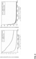
- FIG. 6A and FIG. 6B illustrate example performance of BitNet and LeNet-FP32. That is, FIG. 6A and FIG. 6B show performance of BitNet in comparison to LeNet-FP32 on the MNIST and CIFAR-10 datasets.
- the left panels of each of FIG. 6A and FIG. 6B show the validation error % and the right panel shows the negative log likelihood over training iterations.
- the final validation error is shown in parenthesis.
- the learning rate ⁇ is halved after each epoch that is 250 iterations for MNIST and 200 iterations for CIFAR-10.
- the regularization in BitNet may lead to significantly faster learning.
- the validation error of BitNet reduces more rapidly than LeNet-FP32.
- the validation error of the resulting BitNet after 100 epochs is 2% lower than LeNet-FP32.
- BitNet achieves an error of 5.25% on the test set, whereas LeNet-FP32 achieves error 7.3%.
- BitNet takes roughly half as many iterations as the baseline.
- FIG. 7 illustrates a number of bits used for representing the parameters of each layer of a CNN. That is, FIG. 7 shows the change in the number of bits over training iterations. It can be seen that the number of bits converges within the first five epochs. It can also be observed that the gradient with respect to the bits quickly goes to zero.
- FIG. 8A and FIG. 8B show the impact on performance and compression on the MNIST and CIFAR-10 data, respectively.
- FIG. 8A and FIG. 8B show sensitivity of the test error and compression ratio to the hyperparameters for BitNet for the MNIST and CIFAR-10 datasets, respectively.
- BitNet uses only 2-bits per layer, with a test error of 13.09% in MNIST, a small degradation in exchange for a 16x compression.
- This approach provides some flexibility in limiting the bit-width of parameters and gives an alternative way of arriving at the binary or ternary networks studied in previous work.
- Table 1 shows the results for the MNIST dataset at the end of 30 epochs. TABLE 1 MNIST # Test Error % Num. Params. Compr. Ratio 30 1x1 1x1 30 3x3 1x1 30 3x3 2x2 30 5x5 4x4 50 5x5 4x4 Dense 500 Nodes Dense 500 Nodes Classify 10 Labels 4 11.16 268K 6.7 5 6 7 6 5 10.46 165K 5.72 5 6 6 6 5 6 9.12 173K 5.65 5 6 6 6 6 5 7 8.35 181K 5.75 5 5 6 6 6 6 5 8 7.21 431K 5.57 5 6 5 6 6 6 7 5 CIFAR-10 # Test Error % Num. Params. Compr.
- the first column of Table 1 denotes the number of total layers. Test error is evaluated on a test set (i.e., data that was not seen by DNN 106 during training) and the error measure is the fraction of incorrect answers.
- the compression ratio (Compr. Ratio) is the ratio to the average number of bits used by BitNet. The columns to the right of the compression ratio specify the architecture and the number of bits in the final BitNet model. In each table, the last row contains the full architecture, where the columns read left to right is the neural architecture. In rows above the last row, some of these layers are omitted to train a smaller DNN.
- the heads have the format of P-Q-R where P is the number of convolutional filters, Q is the size of each filter, R is the size of the max pooling that is done after filtering. In the case of Dense layers (i.e., fully-connected layers), it just means the number of neurons.
- the BitNet started with four layers, whose performance was shown in the previous section.
- the test error decreases steadily without any evidence of overfilling.
- the number of bits and the compression ratio are not affected significantly by the architecture and seem to be a strong function of the data and hyperparameters.
- the test error is reduced by additional convolutional as well as dense layers. The addition of 1x1 filters (corresponding to global scaling) may reduce the test error as well, while not increasing the number of parameters in comparison to the addition of dense layers.
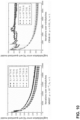
- FIG. 9 shows an example of the performance of BitNet on the MNIST dataset. Particularly, FIG. 9 shows validation error percentage versus iterations of BitNet compared to LeNet-FP32 over minibatches. The final validation error is shown in parenthesis in FIG. 9 .
- the learning rate ⁇ is multiplied by 0.1 after every epoch.
- the left panel of FIG. 9 shows that BitNet may exhibit faster learning similar to using exponential penalty.
- FIG. 10 illustrates example performance of BitNet over different coefficients for linear bit penalty for the MNIST and CIFAR-10 datasets. Specifically, the right panel of FIG. 10 shows that larger values of ⁇ 2 leads to instability and poor performance, whereas a smaller value of ⁇ 2 leads to a smooth learning curve.
- this disclosure describes a flexible tool for training compact DNNs given an indirect specification of the total number of bits available on the target device.
- This disclosure presents a formulation that incorporates such constraints as a regularization on the traditional classification loss function. This formulation is based on controlling the expressive power of the network by dynamically quantizing the range and set of values that the parameters can take.
- the experiments described herein showed faster learning in terms of training and testing errors in comparison to an equivalent unregularized network.
- the robustness of our approach was also shown with increasing depth of the neural network and various hyperparameters.
- Our experiments showed that BitNet may have an indirect relationship to the global learning rate.
- BitNet can be interpreted as having a dynamic learning rate per parameter that depends on the number of bits. In that sense, bit regularization is related to dynamic learning rate schedulers such as AdaGrad. In some examples, machine learning system 104 may anneal the constraints to leverage fast initial learning combined with high precision fine tuning. In that sense, BitNet can be interpreted as having a joint-optimization to learn a representation of the training data and system architecture.
- the previous section of this disclosure described methods to train a DNNs such that the bit precision is part of the parameters in the training procedure.
- the previous section of this disclosure described optimization of bit precision as part of the training phase.
- the resulting DNN may have different bit precisions for the different DNN layers. Benefits may include lower memory footprint, faster learning, and potentially higher algorithmic performance.
- this disclosure presents additional details related to processing embodiments and their relationships to training and inference.
- this disclosure describes (1) how system architecture parameters may be used within BitNet selection of DNN compositions and (2) how system architecture parameters may be used to distribute processing for the trained DNN.
- system architecture to mean a set of the processing hardware (and associated software stack) to train one or more DNNs and/or execute the one or more DNNs in inference mode.
- the processing hardware may include virtual machines that act like physical hardware.
- a system architecture comprises one or more processors (e.g., CPUs, GPUs, FPGAs, DSPs, or virtualized representations thereof) that support training of BitNet DNNs.
- processors e.g., CPUs, GPUs, FPGAs, DSPs, or virtualized representations thereof
- the same system architecture can be used to run the trained DNN in inference mode.
- an alternate system architecture can be used.
- one or more BitNet DNNs may be trained on a first system architecture (e.g., a cloud computing system) and then used in inference mode on a second, different system architecture (e.g., a mobile device).
- This disclosure uses the term neural network software architecture to mean a system composed of one or more DNNs and the compositions of those DNNs.
- a neural network software architecture may include multiple separate DNNs that may interact.
- this disclosure describes techniques related to methods of DNN training in which system architecture inputs are used to select a composition the DNN model. Additional techniques of this disclosure include methods in which DNN processing (both training and inference) is distributed among processors in a system architecture.
- FIG. 11 is an example neural network software architecture 1100 composed of a hierarchy of layers, where each of the layers is a DNN. That is, FIG. 11 shows an example neural network software architecture composed of a hierarchy of neural networks.
- sensor inputs to neural network software architecture 1100 are video data, audio data, and a depth map.
- the output of neural network software architecture 1100 is a classification of an activity, detected from an analysis of the video, audio, and depth map.
- an application of neural network software architecture 1100 may be human gesture recognition.
- a human developer or a computing system may select neural network software architecture 1100.
- an 8-bit CNN 1102 is selected for the video data.
- the high-precision weights of CNN 1102 are each 8 bits.
- the precision-optimized weights of CNN 1102 may be updated to have bit precisions less than 8.
- a 4-bit CNN 1104 followed by a 32-bit LSTM (Long Short-Term Memory neural network) 1106 is selected for the audio data.
- the high-precision weights of CNN 1104 are each 4 bits and the high-precision weights of LSTM 1106 are each 32 bits.
- the precision-optimized weights of CNN 1104 and LSTM 1106 may be updated to have bit precisions less than 4 and 32, respectively.
- a 1-bit BNN 1108 is selected for the depth map.
- the three streams generated by CNN 1102, LSTM 1106, and BNN 1108 are fed into an 8-bit MLP (multi-layer perceptron) 1110 to generate the activity classification output.
- the high-precision weights of MLP 1110 may each be 8 bits.
- the precision-optimized weights of MLP 1110 may be updated to have bit precisions less than 8.
- the video data may comprise 2-dimensional imagery with different color planes (red, green, blue), and are typically 8-bits per pixel.
- the audio data may comprise a single dimensional stream and are typically 16-bits per sample. Audio processing can include feature extraction (e.g., with CNN 1104) and then speech analysis (e.g., with LSTM 1106).
- the depth map may comprise a 2-dimensional mask with pixel values representing distance from a sensor (e.g., camera).
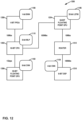
- FIG. 12 is an example system architecture 1200 comprising a heterogeneous set of processors.
- the processors include a CPU 1202, a GPU 1204, a GPU 1206, a FPGA 1208, and a DSP 1210.
- Each processor has different bit-precision support.
- Example supported bit precisions may include 8-bit and 1-bit precision (integer) and 32-bit and 64-bit (floating point).
- the different processor hardware can process the DNN computation differently (e.g., with different levels of parallelism and organization of memory) to support different size, weight, and power (SWaP) offerings.
- the processors may be connected in a network. In the example of FIG. 12 , each network connection has different bandwidth availability, for example, 10Mbps, 100Mbps, and 1Gbps.
- router 1212 that directs traffic but does not perform any computation for any DNN.
- the network bandwidth availability sets the communication limits between processors, and as such, may have an impact on how the DNNs are trained and processed during inference.
- machine learning system 104 may first review the system architecture on which neural network software architecture 1100 needs to operate in inference mode. For example, machine learning system 104 may determine that, for a 1-bit BNN, the best processor would be an FPGA because FPGAs have fine grain programmable units that can support binary operations. In comparison, LSTMs may require higher precision because of its time series analysis. Machine learning system 104 may also consider the amount of network bandwidth required to support the communications between the different layers of the DNN. For example, video processing may require more communication bandwidth compared to audio processing. Other examples of system architecture parameters may include memory footprint (e.g., l-bit BNN has a smaller memory requirement than 8-bit CNN).
- the system architecture parameters are used to map the neural network software architecture to the appropriate processors in the system architecture.
- machine learning system 104 of computing system 100 ( FIG. 1 ) map the neural network software architecture to appropriate processors in the system architecture.
- Machine learning system 104 may use a cost function to select the best mapping (e.g., a best fit algorithm can be use).
- the cost function can be one of size, weight, power and cost (SWaPC).
- SWaPC size, weight, power and cost
- machine learning system 104 may use the cost function to select a mapping that provides a lower system SWaPC.
- machine learning system 104 may evaluate various potential mappings of DNNs in a neural network software architecture to processors in a hardware architecture.
- Machine learning system 104 may use a mapping cost function to select a mapping of DNNs in the neural network software architecture to processors in the hardware architecture.
- FIG. 12 shows an example mapping of a neural network software architecture to a system architecture. More specifically, machine learning system 104 may map 8-bit CNN 1102 of FIG. 11 to 32-bit floating point CPU 1206 of FIG. 12 . The same 8-bit CNN, if mapped to an FPGA, may incur higher computation resources (e.g., higher usage of memory and a FPGA fabric to support floating point computations). Furthermore, in the example of FIG. 12 , machine learning system 104 may map 1-bit BNN 1108 to 1-bit FPGA 1208, map 8-bit MLP 1110 to 16-bit CPU 1202, map 32-bit LSTM 1106 to 64-bit floating point GPU 1204, and map 4-bit CNN 1104 to 8-bit DSP 1210. After machine learning system 104 maps a DNN to a processor, the processor may execute the DNN. For instance, in the example of FIG. 12 , GPU 1206 may execute CNN 1102.
- the system architecture parameters serve as an input to a BitNet DNN (e.g., DNN 106 ( FIG. 1 ) to select the appropriate neural network software architecture and a mapping of DNNs in the neural network software architecture to processors in a hardware architecture.
- DNN 106 may be a BitNet DNN that receives a description of a hardware architecture and a description of a problem that a neural network software architecture is designed to solve.
- the output of DNN 106 may be an appropriate neural network software architecture for the problem that the neural network software architecture is designed to solve and a mapping of DNNs in the neural network software architecture to processors in the hardware architecture.
- DNN 106 may be trained using existing examples of hardware architectures and problem descriptions.
- a BitNet DNN's ability to target multiple bit-precisions may allow for more efficient mapping to available hardware resources and may be especially useful for heterogeneous sets of processors.
- machine learning system 104 may be able to train multiple versions of the same BitNet DNN based on the same input data but so that the different versions of the same BitNet DNN have different bit depths.
- P represents a set of hardware parameters for a hardware architecture
- r ( b, P ) is a function, termed a resource function herein, that takes as parameters the precision-optimized bit depths b of the BitNet DNN and also the set of hardware parameters P.
- the resource function r produces higher values when the precision-optimized bit depths in any layer of the BitNet DNN exceeds a limit indicated in the set of hardware parameters P.
- the resource function r may be a step function that produces a value of 0 if the bit depths of each layer of the BitNet DNN are below the limit and produces a value of 1 if the bit depth of any layer of the BitNet DNN is above the limit.
- the resource function r may produce progressively larger values the more the precision-optimized bit depths exceed the limit.
- the limit is a memory requirement.
- the limit may be on a total amount of memory required for storage of the precision-optimized weights b (e.g., a total amount of memory required for storage of b must be less than 32 kilobytes).
- the limit may be on a maximum amount of storage that can be used for storage of precision-optimized weights of a single layer of the BitNet DNN (e.g., no layer can have precision-optimized weights that are each greater than 4 bits).
- the resource function r may return a value based on whether the weights are read-boundary aligned. For instance, if a single memory read operation returns 8 bits, two memory read operations may be required to return a 9-bit weight.
- the resource function r may return a low value if the precision-optimized weights are read-boundary aligned.
- priority may be put on minimizing the number of read operations and therefore reducing potential energy consumption and delays associated with read operations.
- machine learning system 104 may use the loss function expressed in Equation (34), below.
- ⁇ 3 is a third hyperparameter and r ( b, P ) may be defined as above.
- the loss function of Equation (34) may allow bit depths to be accounted for separately from the hardware parameters P.
- the loss function may include one or more additional factors with additional hyperparameters and additional functions based on b and various hardware factors.
- the loss function may be able to take into account various hardware parameters when training a BitNet DNN.
- the techniques here may allow machine learning system 104 to find the optimal DNN performance given a set of hardware resources, such as the processors and communication links of FIG. 12 . Computation during the training phase can also be mapped similarly to the appropriate hardware for testing in the appropriate hardware that supports the selected bit-precision.
- the techniques described herein may also be applicable to hardware resources within a processor.
- SoC System-on-Chip
- the techniques can be used similarly, using system architecture parameters (in this case, they would be related to the SoC) to map a neural network software architecture to SoC resources.
- system architecture comprises or consists of a bank of FPGAs
- machine learning system 104 may use DNN 106 to select the appropriate FPGA resources (e.g., allocating FPGA lookup tables (LUTs) and memory) to obtain the best and optimal DNN performance based on available hardware.
- LUTs allocating FPGA lookup tables
- FIG. 12 shows an example mapping of a neural network software architecture to system architecture resources.
- this disclosure described an AI system that can manage and anticipate its resource needs.
- the AI system may anticipate its resource needs by determining which parts of the neural network software architecture would be most efficiently executed on the processors available in a given system architecture.
- an engineer or computing system may identify a plurality of different scenarios.
- different scenarios may be different system architectures.
- different scenarios may involve the same set of processors but with differences in other parameters, such as available bandwidth, available remaining battery life, remaining allocable memory space, processor workload, and so on.
- machine learning system 104 may train multiple versions of the same neural network software architecture using the techniques of this disclosure based on the different scenarios.
- each version of the neural network software architecture may be tailored for use with a different anticipated scenario.
- a BitNet training method can be invoked to map the neural network software architecture to a new set of system architecture parameters. Specifically, a new mapping is performed on the neural network software architecture (e.g., neural network software architecture 1100 of FIG. 11 ) to a new system architecture (e.g., a subset of processors in FIG. 12 ). For instance, in the example of FIG. 12 , if GPU 1206 becomes unavailable, mapping module 122 may deploy on the remaining processors of system architecture 1200 (i.e., hardware architecture) a version of neural network software architecture 1100 tailored for use in the scenario in which GPU 1206 is unavailable.
- system architecture 1200 i.e., hardware architecture
- CNN 1102 and LSTM 1106 may both be mapped to GPU 1204.
- One aspect here is the combination of BitNet training with a dynamic set of system architecture parameters.
- the cost function for BitNet may be based on a dynamic set of system architecture parameters (e.g., a loss function).
- the cost function may be the loss function as described previously as Equation (34), where ⁇ 1 and ⁇ 2 are set based to optimize one of size, weight, power and cost (SWaPC) of the hardware architecture 1200.
- BitNet training can be used to arrive at multiple neural network software architectures for a set of typical configurations. For example, in reference to FIG. 12 , if router 1212 has periodic reductions in bandwidth (e.g., during different period of time when there is network congestion), BitNet may generate two neural network software architectures during training (one that maps a DNN to a system using router 1212, and one that maps the DNN to a system without router 1212). As such, this process is analogous to fat-binaries, in which multiple statically compiled program can be selected at runtime based on dynamic conditions. In our case, the BitNet DNN selects neural network software architectures appropriate to the available hardware. In other words, DNN 106 may select an appropriate previously-prepared neural network software architecture from among a plurality of previously-prepared neural network software architectures. Each DNN in each of the previously-prepared neural network software architecture is already trained.
- selected weights are selected based on a joint optimization of DNN performance and hardware resources.
- this disclosure describes hardware parameters P that may be updated during training to affect the selection of the annealing constraints.
- the selection of hardware parameters P during training allows for a pareto-optimal selection of hardware resources with respect to size, weight, and power, for example.
- Such approach in dynamic selection of hardware parameters serves as a design tradeoff method for a designer, using the loss function as a joint-optimization of machine learning performance and hardware resource.
- This disclosure describes a loss function that uses a correspondence between the bit-precision and hardware parameters, with respect to equation (34) and in reference to r ( b, P ) function. It is understood that the correspondence can be a similar mapping of machine learning hyper parameters (e.g. bit precision, learning rate, DNN depth, fusion layers, activation, learning algorithm) to hardware parameters, to enable a joint-optimization. It is also understood then that the correspondence can be other similar mapping of machine learning parameters to other physical constraints (e.g. environmental, data biases) that influence the DNN training, wherein a joint-optimization can be performed similarly, as in equation (34).
- machine learning hyper parameters e.g. bit precision, learning rate, DNN depth, fusion layers, activation, learning algorithm
- the correspondence can be other similar mapping of machine learning parameters to other physical constraints (e.g. environmental, data biases) that influence the DNN training, wherein a joint-optimization can be performed similarly, as in equation (34).
- this disclosure describes an example in a space-borne application.
- This example uses a spaceborne application because there are strict limitations on available SWaP and communication bandwidth.
- Small satellites such as cube-sats may only have 10 ⁇ 10 ⁇ 10cm and 1.33Kg weight.
- Cube-sats typically operate as distributed swarms, each with different set of sensors.
- Each cube-sat may have a different set of processors.
- machine learning system 104 FIG. 1
- a BitNet DNN may be used to distribute and map the DNN inference computation among the cube-sats.
- the BitNet DNN can be used to re-train and distribute the DNN computation to the currently available cube-sat hardware.
- the BitNet DNN e.g., DNN 106
- the BitNet DNN can target specific bit-precisions
- the BitNet DNN can optimally map other DNNs to system resources. With a changing set of system resources, DNN 106 can dynamically reselect a different neural network software architecture to match available hardware.
- the BitNet cost function for mapping can be one of resiliency.
- BitNet DNN 106 can be used to find the optimal network configuration, among the available cube-sat hardware. For example, point-to-point network communication between cube-sats can be made in a way to support the most optimal DNN performance.
- AI systems have been demonstrated in a myriad of applications, from search engines to autonomous vehicles.
- the AI systems may use DNN algorithms that have recently shown outstanding performance in learning intricate relationships in multi-dimensional data.
- current AI systems typically do not have the ability to learn beyond what they were prepared for in advance. In situations where complete details are often unknown in advance, current AI systems are not able to react quickly and adapt to dynamic circumstances.
- the traditional approach may require taking the system offline for retraining/re-programming. This process may be expensive and time-consuming, not to mention disruptive or infeasible for certain tasks.
- an AI system that can continue learning while more or less simultaneously performing inference. More specifically, it may be advantageous for an AI system to support simultaneously learning and inference in an efficient manner (e.g., from a learning perspective, and from a power/performance perspective). Such an AI system may autonomously self-reconfigure on the fly, including adjustment of hyper-parameters such as a learning rate.
- This disclosure presents an AI system that may (a) anticipate its learning needs, and (b) may dynamically and proactively manage its operation/resources.
- the AI system may select or search for optimal DNN parameters without training to full convergence.
- the techniques here may decouple the training and DNN structure optimization tasks, which may break away from the conventional approach that relies on iterative model selection and training to find a set of hyper-parameters that leads to optimal performance on a given dataset.
- the techniques here may be applicable in many areas because the techniques may apply to the basic ability for the AI systems to select its own infrastructure (learning approach, software/hardware, etc.).
- the techniques may enable AI systems to be adaptive at the edge by providing an approach to tradeoff algorithmic performance and hardware SWaP (size, weight and power).
- SWaP size, weight and power
- the techniques here may be useful for applications like self-driving car and robots, where the autonomous aspects are enhanced with the ability to self-reconfigure while improving its learning capability.
- the techniques here may enable powerful DNNs for resource-constrained environments, such as mobile smartphone devices.
- the techniques here may be a valuable tool in other areas such as cybersecurity, where advance information on the cyber-attack is unknown (and taking the system offline for retraining is not a viable option).
- the techniques here may be useful for user customization/individualization, where the AI system self-reconfigure based on user inputs.
- the system gathers inputs from sensors from external environment and internal operations.
- the sensors may generate various types of data, such as data indicating availability status of processors, up/down states of communication links, availability of electrical energy, temperature, remaining battery power, remaining memory space, need for real-time performance, and so on.
- the system may then learn from these input sensor data.
- This disclosure extends the "react" aspects where the system reconfigures itself (algorithm, software, hardware, etc.) based on what it senses and what it learns to do.
- DNN 106 may be implemented as a BitNet DNN that takes hardware parameters as input and outputs a neural network software architecture that includes one or more DNNs mapped to processors of a hardware architecture.
- the one or more DNNs in the neural network software architecture may themselves be BitNet DNNs.
- the one or more DNNs in the neural network software architecture may be pretrained.
- machine learning system 104 may train one or more of the DNNs in the neural network software architecture to meet requirements of specific processors after DNN 106 selects the neural network software architecture and the mapping.
- DNN 106 may continue to update the neural network software architecture as DNN 106 receives new inputs from the sensors.
- machine learning system 104 may cause machine learning system 104 to reconfigure DNN 106 based on the selection or search of optimal learning parameters. More specifically, the technique includes the selection of appropriate DNN parameters (e.g., weights), and not just hardware/software parameters (e.g., processor operating frequency, software processing needs, available battery power). With respect to DNN training, the techniques for selecting or searching for optimal DNN parameters may be done without training to full convergence, because in one example, a DNN with lower bit precision can be an alternative neural network that approximates the computation of a higher precision neural network.
- DNN parameters e.g., weights
- hardware/software parameters e.g., processor operating frequency, software processing needs, available battery power
- This technique combines the following: (a) system reconfiguration, (b) selection and optimization of DNN learning parameters, and (c) without fully training the DNN, whereby training can essentially stop when the BitNet trained neural network has reached a predefined performance that approximates a neural network trained with higher bit-precision.
- bitNet trained neural network There are a number of options for low SWaP hardware and circuit embodiments for a BitNet trained neural network.
- certain processors or hardware accelerators can be turned on when needed to support different DNN computational needs.
- certain circuit fabrics can be turned on (configured) when needed.
- certain banks of memory can be utilized to provide higher bandwidth to stored parameters. Additional tradeoffs in time/energy associated with storage and movement of data can be configured to support fast gradient evaluations (local and global). Additional circuits (neuromorphic, analog and memristors) can be used.
- Analog processors can select different bit-precision to address manufacturing variance in advanced nanoelectronics.
- computing system 100 may enable autonomous changes of its own implementation, optimized for SWaPC (size, weight, power, cost) and effectiveness (throughput, latency, functional optimality).
- SWaPC size, weight, power, cost
- effectiveness throughput, latency, functional optimality
- the BitNet DNN techniques of this disclosure may enable lifelong learning with architectural evolution.
- adjustments on both system (hardware and software) and learning (learning rate, DNN depth, fusion layers) may be performed dynamically based on system needs.
- the hardware may support both on-line learning and near-simultaneously inference, supported by our DNN selection algorithms that do not need to train to convergence.
- computing system 100 may deterministically select an appropriate neural network software architecture (using selection algorithms described in this disclosure), configure the hardware as appropriate, and continue operating without being taken off-line for training.
- this disclosure describes a method for selecting/switching DNN contexts.
- Capabilities provided by AI systems may be important for agile systems. New AI systems may adapt to context from different types of data simultaneously (EO, IR, radar, etc.). It may be desirable for these platforms to support on-line training in the field with limited power and size budgets.
- the techniques here may be especially effective on network structure optimization for diverse, multi-modal data.
- Agile systems may use learning approaches that are unsupervised and continuous, and as such, techniques of this disclosure may adapt continuously to respond to changing environmental cues.
- Computing system 100 may address issues on catastrophic learning loss by enabling fast structure (e.g., neural network software architecture) selection and optimization with multi-modal composition of DNNs, e.g., using the previously described approach using dynamic parameters without training to full convergence, as described for FIG. 12 .
- Such an AI system may also be more resilient to adversarial attack.
- computing system 100 may prevent an adversary from learning its AI behavior, by enabling computing system 100 to self-reconfigure its learning approach (e.g., using different hyperparameters in the loss function described in Equation 16 to arrive at a new set of DNN parameters, with different bit-precision and range of values).
- learning approach e.g., using different hyperparameters in the loss function described in Equation 16 to arrive at a new set of DNN parameters, with different bit-precision and range of values.
- From a cyber-security perspective such a learning approach may be resilient to adversarial targeting.
- An enabler for the techniques of this disclosure is for the Al system to support system adaptation at machine speed.
- the Al system may automatically change with version of the DNN is active in real time (e.g., based on changes to hardware architecture parameters, based on the detection of a cybersecurity threat, and so on.) This may enable more effective detection, learning, and responses at low latency (e.g., sense, learn, react). Furthermore, this may be important for many autonomous systems and cybersecurity systems where detection and countermeasures must be deployed efficiently and quickly.
- FIG. 13 is a flowchart illustrating an example operation of a machine learning system, in accordance with a technique of this disclosure.
- machine learning system 104 may obtain system architecture parameters (1300).
- the system architecture parameters may include data describing processors in a system architecture.
- the system architecture parameters include data describing communication links amount processors in the system architecture.
- the system architecture parameters include data indicating current conditions of computing resources in the system architecture.
- machine learning system 104 may obtain the system architecture parameters from machine learning system 104 ( FIG. 1 ).
- machine learning system 104 may determine, based on the system architecture parameters, a neural network software architecture and a mapping of DNNs in the neural network software architecture to processors of the system architecture (1302). For example, machine learning system 104 may use DNN 106 to determine the neural network software architecture and the mapping based on the system architecture parameters. Thus, a neural network software architecture and a mapping of DNNs in the neural network software architecture to processors of the system architecture is an output of DNN 106. In this example, during training of DNN 106, machine learning system 104 may use a cost function that assigns cost values to potential neural network software architectures and mappings of DNNs based on one or more of size, weight, power and cost, as defined using the system architecture parameters.
- machine learning system 104 may use pretrained DNNs in the neural network software architecture.
- machine learning system 104 may perform additional training iterations on the pretrained DNNs using different values of hyperparameters (e.g., ⁇ 1 ⁇ 2 , ⁇ 3 , etc.) in the loss function than were used in generating the pretrained DNNs in order to optimize the pretrained DNNs for the processors of the hardware architecture to which the DNNs are mapped.
- hyperparameters e.g., ⁇ 1 ⁇ 2 , ⁇ 3 , etc.
- Machine learning system 104 may repeat actions (1300) and (1302) multiple times based on different system architecture parameters to determine multiple versions of the neural network software architecture and potentially different mappings of DNNs to processors of system architectures indicated by the system architecture parameters.
- processors mapped to the DNNs of the neural network software architecture may execute the DNNs of the neural network software architecture (1304). In some examples, the processors may execute the DNNs in an evaluate mode. In some examples, the processor may continue training the DNNs.
- a computing system includes a memory for storing a set of weights of the DNN.
- the DNN includes a plurality of layers. For each layer of the plurality of layers, the set of weights includes weights of the layer and a set of bit precision values includes a bit precision value of the layer.
- the weights of the layer are represented in the memory using values having bit precisions equal to the bit precision value of the layer.
- the weights of the layer are associated with inputs to neurons of the layer.
- the computing system includes processing circuitry for executing a machine learning system configured to train the DNN. Training the DNN comprises optimizing the set of weights and the set of bit precision values.
- processors including one or more microprocessors, digital signal processors (DSPs), application specific integrated circuits (ASICs), field programmable gate arrays (FPGAs), or any other equivalent integrated or discrete logic circuitry, as well as any combinations of such components.
- DSPs digital signal processors
- ASICs application specific integrated circuits
- FPGAs field programmable gate arrays
- processors may generally refer to any of the foregoing logic circuitry, alone or in combination with other logic circuitry, or any other equivalent circuitry.
- a control unit comprising hardware may also perform one or more of the techniques of this disclosure.
- Such hardware, software, and firmware may be implemented within the same device or within separate devices to support the various operations and functions described in this disclosure.
- any of the described units, modules or components may be implemented together or separately as discrete but interoperable logic devices. Depiction of different features as modules or units is intended to highlight different functional aspects and does not necessarily imply that such modules or units must be realized by separate hardware or software components. Rather, functionality associated with one or more modules or units may be performed by separate hardware or software components, or integrated within common or separate hardware or software components.
- Computer-readable media may include computer-readable storage media, which corresponds to a tangible medium such as data storage media, or communication media including any medium that facilitates transfer of a computer program from one place to another, e.g., according to a communication protocol.
- computer-readable media generally may correspond to (1) tangible computer-readable storage media which is non-transitory or (2) a communication medium such as a signal or carrier wave.
- Data storage media may be any available media that can be accessed by one or more computers or one or more processors to retrieve instructions, code and/or data structures for implementation of the techniques described in this disclosure.
- Computer readable storage media may include random access memory (RAM), read only memory (ROM), programmable read only memory (PROM), erasable programmable read only memory (EPROM), electronically erasable programmable read only memory (EEPROM), flash memory, a hard disk, a CD-ROM, a floppy disk, a cassette, magnetic media, optical media, or other computer readable media.
Landscapes
- Engineering & Computer Science (AREA)
- Physics & Mathematics (AREA)
- Theoretical Computer Science (AREA)
- Health & Medical Sciences (AREA)
- Life Sciences & Earth Sciences (AREA)
- Biomedical Technology (AREA)
- Biophysics (AREA)
- General Health & Medical Sciences (AREA)
- Data Mining & Analysis (AREA)
- Evolutionary Computation (AREA)
- Computational Linguistics (AREA)
- Molecular Biology (AREA)
- Computing Systems (AREA)
- General Engineering & Computer Science (AREA)
- General Physics & Mathematics (AREA)
- Mathematical Physics (AREA)
- Software Systems (AREA)
- Artificial Intelligence (AREA)
- Neurology (AREA)
- Machine Translation (AREA)
Applications Claiming Priority (3)
| Application Number | Priority Date | Filing Date | Title |
|---|---|---|---|
| US201862644715P | 2018-03-19 | 2018-03-19 | |
| US201862645358P | 2018-03-20 | 2018-03-20 | |
| US16/133,446 US11429862B2 (en) | 2018-03-20 | 2018-09-17 | Dynamic adaptation of deep neural networks |
Publications (2)
| Publication Number | Publication Date |
|---|---|
| EP3543917A1 EP3543917A1 (en) | 2019-09-25 |
| EP3543917B1 true EP3543917B1 (en) | 2024-01-03 |
Family
ID=65904040
Family Applications (1)
| Application Number | Title | Priority Date | Filing Date |
|---|---|---|---|
| EP19163921.0A Active EP3543917B1 (en) | 2018-03-19 | 2019-03-19 | Dynamic adaptation of deep neural networks |
Country Status (3)
| Country | Link |
|---|---|
| EP (1) | EP3543917B1 (https=) |
| JP (3) | JP2019164793A (https=) |
| KR (1) | KR102329590B1 (https=) |
Families Citing this family (92)
| Publication number | Priority date | Publication date | Assignee | Title |
|---|---|---|---|---|
| WO2018125928A1 (en) | 2016-12-29 | 2018-07-05 | DeepScale, Inc. | Multi-channel sensor simulation for autonomous control systems |
| WO2018176000A1 (en) | 2017-03-23 | 2018-09-27 | DeepScale, Inc. | Data synthesis for autonomous control systems |
| US11893393B2 (en) | 2017-07-24 | 2024-02-06 | Tesla, Inc. | Computational array microprocessor system with hardware arbiter managing memory requests |
| US11157441B2 (en) | 2017-07-24 | 2021-10-26 | Tesla, Inc. | Computational array microprocessor system using non-consecutive data formatting |
| US11409692B2 (en) | 2017-07-24 | 2022-08-09 | Tesla, Inc. | Vector computational unit |
| US10671349B2 (en) | 2017-07-24 | 2020-06-02 | Tesla, Inc. | Accelerated mathematical engine |
| US12307350B2 (en) | 2018-01-04 | 2025-05-20 | Tesla, Inc. | Systems and methods for hardware-based pooling |
| US11561791B2 (en) | 2018-02-01 | 2023-01-24 | Tesla, Inc. | Vector computational unit receiving data elements in parallel from a last row of a computational array |
| KR102329590B1 (ko) * | 2018-03-19 | 2021-11-19 | 에스알아이 인터내셔널 | 딥 신경망들의 동적 적응 |
| US11429862B2 (en) | 2018-03-20 | 2022-08-30 | Sri International | Dynamic adaptation of deep neural networks |
| US11215999B2 (en) | 2018-06-20 | 2022-01-04 | Tesla, Inc. | Data pipeline and deep learning system for autonomous driving |
| CN108985920A (zh) | 2018-06-22 | 2018-12-11 | 阿里巴巴集团控股有限公司 | 套现识别方法和装置 |
| US11361457B2 (en) | 2018-07-20 | 2022-06-14 | Tesla, Inc. | Annotation cross-labeling for autonomous control systems |
| US11636333B2 (en) | 2018-07-26 | 2023-04-25 | Tesla, Inc. | Optimizing neural network structures for embedded systems |
| US11562231B2 (en) | 2018-09-03 | 2023-01-24 | Tesla, Inc. | Neural networks for embedded devices |
| KR20250078625A (ko) | 2018-10-11 | 2025-06-02 | 테슬라, 인크. | 증강 데이터로 기계 모델을 훈련하기 위한 시스템 및 방법 |
| US11196678B2 (en) | 2018-10-25 | 2021-12-07 | Tesla, Inc. | QOS manager for system on a chip communications |
| WO2020102888A1 (en) * | 2018-11-19 | 2020-05-28 | Tandemlaunch Inc. | System and method for automated precision configuration for deep neural networks |
| US11816585B2 (en) | 2018-12-03 | 2023-11-14 | Tesla, Inc. | Machine learning models operating at different frequencies for autonomous vehicles |
| US11537811B2 (en) | 2018-12-04 | 2022-12-27 | Tesla, Inc. | Enhanced object detection for autonomous vehicles based on field view |
| US11610117B2 (en) | 2018-12-27 | 2023-03-21 | Tesla, Inc. | System and method for adapting a neural network model on a hardware platform |
| US10997461B2 (en) | 2019-02-01 | 2021-05-04 | Tesla, Inc. | Generating ground truth for machine learning from time series elements |
| US11150664B2 (en) | 2019-02-01 | 2021-10-19 | Tesla, Inc. | Predicting three-dimensional features for autonomous driving |
| US11567514B2 (en) | 2019-02-11 | 2023-01-31 | Tesla, Inc. | Autonomous and user controlled vehicle summon to a target |
| US10956755B2 (en) | 2019-02-19 | 2021-03-23 | Tesla, Inc. | Estimating object properties using visual image data |
| US11657118B2 (en) * | 2019-05-23 | 2023-05-23 | Google Llc | Systems and methods for learning effective loss functions efficiently |
| CN112668362B (zh) * | 2019-10-15 | 2023-06-16 | 浙江中正智能科技有限公司 | 一种动态优化类代理的人证比对模型训练方法 |
| CN114556380B (zh) * | 2019-10-17 | 2026-01-30 | 富士通株式会社 | 机器学习程序、机器学习方法以及机器学习装置 |
| US11775611B2 (en) | 2019-11-01 | 2023-10-03 | Samsung Electronics Co., Ltd. | Piecewise quantization for neural networks |
| CN111079523B (zh) * | 2019-11-05 | 2024-05-14 | 北京迈格威科技有限公司 | 物体检测方法、装置、计算机设备和存储介质 |
| CN112784954B (zh) * | 2019-11-08 | 2025-07-29 | 华为技术有限公司 | 确定神经网络的方法和装置 |
| US11836490B2 (en) * | 2019-11-14 | 2023-12-05 | Nvidia Corporation | Kernel coefficient quantization |
| US12039430B2 (en) * | 2019-11-15 | 2024-07-16 | Samsung Electronics Co., Ltd. | Electronic device and method for inference binary and ternary neural networks |
| CN110942094B (zh) * | 2019-11-26 | 2022-04-01 | 电子科技大学 | 一种基于范数的对抗性样本检测分类方法 |
| WO2021112335A1 (ko) * | 2019-12-06 | 2021-06-10 | 주식회사 애자일소다 | 생성적 적대 신경망 기반의 분류 시스템 및 방법 |
| KR102093080B1 (ko) * | 2019-12-06 | 2020-04-27 | 주식회사 애자일소다 | 레이블 데이터 및 비레이블 데이터를 이용한 생성적 적대 신경망 기반의 분류 시스템 및 방법 |
| CN112926174B (zh) * | 2019-12-06 | 2024-07-09 | 富益成科技有限公司 | 电池智能分流的控制方法及系统 |
| US11899765B2 (en) | 2019-12-23 | 2024-02-13 | Dts Inc. | Dual-factor identification system and method with adaptive enrollment |
| US11551145B2 (en) | 2020-02-05 | 2023-01-10 | International Business Machines Corporation | Performance based switching of a model training process |
| WO2021158225A1 (en) * | 2020-02-06 | 2021-08-12 | Hewlett-Packard Development Company, L.P. | Controlling machine learning model structures |
| CN111399933B (zh) * | 2020-02-11 | 2022-05-31 | 福建师范大学 | 一种边缘-云混合计算环境下的dnn任务卸载方法及终端 |
| JP7268069B2 (ja) | 2020-02-21 | 2023-05-02 | アクタピオ,インコーポレイテッド | 学習装置、学習方法、学習プログラム、評価装置、評価方法、および評価プログラム |
| US11586932B2 (en) | 2020-03-10 | 2023-02-21 | International Business Machines Corporation | Model training with variable batch sizing and gradient checkpoint segments |
| CN111401430B (zh) * | 2020-03-12 | 2022-04-01 | 四川大学 | 一种基于双通道深度神经网络的图像在线分类方法 |
| US20230093630A1 (en) * | 2020-03-17 | 2023-03-23 | Interdigital Ce Patent Holdings | System and method for adapting to changing constraints |
| KR102488281B1 (ko) * | 2020-03-30 | 2023-01-13 | 주식회사 모빌린트 | 인공신경망의 활성값 및 가중값의 정밀도를 적응적으로 제어하는 방법 및 그 장치 |
| CN113688851B (zh) * | 2020-05-18 | 2023-09-15 | 华为云计算技术有限公司 | 数据标注方法和装置和精细粒度识别方法和装置 |
| US12015526B2 (en) * | 2020-05-26 | 2024-06-18 | Synopsys, Inc. | Mixed-precision neural networks |
| KR102831990B1 (ko) * | 2020-06-11 | 2025-07-10 | 울산과학기술원 | 이기종 그래픽 프로세서 유닛 클러스터를 이용한 마이크로서비스 기반의 트레이닝 시스템 및 그 동작 방법 |
| CN111738419B (zh) * | 2020-06-19 | 2024-01-12 | 北京百度网讯科技有限公司 | 神经网络模型的量化方法和装置 |
| CN111783957B (zh) * | 2020-07-02 | 2024-05-03 | 厦门美图之家科技有限公司 | 模型量化训练方法、装置、机器可读存储介质及电子设备 |
| CN111831354B (zh) * | 2020-07-09 | 2023-05-16 | 北京灵汐科技有限公司 | 数据精度配置方法、装置、芯片、芯片阵列、设备及介质 |
| JP6992864B1 (ja) | 2020-09-28 | 2022-01-13 | 沖電気工業株式会社 | ニューラルネットワーク軽量化装置、ニューラルネットワーク軽量化方法およびプログラム |
| US12591771B2 (en) | 2020-09-29 | 2026-03-31 | Qualcomm Incorporated | Dynamic quantization for energy efficient deep learning |
| WO2022081260A1 (en) | 2020-10-16 | 2022-04-21 | Starkey Laboratories, Inc. | Hearing device with dynamic neural networks for sound enhancement |
| US12488249B2 (en) * | 2020-10-20 | 2025-12-02 | Samsung Electronics Co., Ltd. | Secure, accurate and fast neural network inference by replacing at least one non-linear activation channel |
| CN114501353B (zh) * | 2020-10-23 | 2024-01-05 | 维沃移动通信有限公司 | 通信信息的发送、接收方法及通信设备 |
| CN112311488A (zh) * | 2020-11-05 | 2021-02-02 | 上海应用技术大学 | 基于小波分解的频谱感知方法 |
| US12159238B2 (en) | 2020-12-10 | 2024-12-03 | International Business Machines Corporation | Automated machine learning model selection |
| GB2602294B (en) * | 2020-12-22 | 2024-05-29 | Imagination Tech Ltd | Compressing a set of coefficients for subsequent use in a neural network |
| US20220253713A1 (en) * | 2021-02-05 | 2022-08-11 | Google Llc | Training neural networks using layer-wise losses |
| KR102314864B1 (ko) * | 2021-03-29 | 2021-10-19 | 주식회사 리트빅 | 차량운전 상태정보를 이용한 에지 딥러닝 기반의 차량 안전운전 시스템 |
| KR20220147398A (ko) * | 2021-04-27 | 2022-11-03 | 삼성전자주식회사 | 인공 지능 모델에 기반하여 데이터를 처리하는 전자 장치 및 그 동작 방법 |
| JP7187065B1 (ja) | 2021-06-25 | 2022-12-12 | 株式会社モルフォ | 計算手法決定システム、計算手法決定方法、及び、計算手法決定プログラム |
| CN113761787B (zh) * | 2021-07-19 | 2024-08-02 | 中南大学 | 基于深度迁移网络的高炉铁水硅含量在线预测方法及系统 |
| WO2023023265A1 (en) | 2021-08-19 | 2023-02-23 | Tesla, Inc. | Vision-based system training with simulated content |
| US12462575B2 (en) | 2021-08-19 | 2025-11-04 | Tesla, Inc. | Vision-based machine learning model for autonomous driving with adjustable virtual camera |
| KR102590993B1 (ko) * | 2021-09-03 | 2023-10-19 | 한국전자기술연구원 | 적응형 배치 프로세싱 방법 및 시스템 |
| CN113872873B (zh) * | 2021-09-29 | 2023-05-02 | 西安交通大学 | 一种适合5g新应用的多场景跨层拥塞控制方法 |
| CN114037055A (zh) * | 2021-11-05 | 2022-02-11 | 北京市商汤科技开发有限公司 | 数据处理系统、方法、装置、设备及存储介质 |
| CN114118384B (zh) * | 2021-12-09 | 2024-06-04 | 安谋科技(中国)有限公司 | 神经网络模型的量化方法、可读介质和电子设备 |
| US20250068890A1 (en) | 2021-12-24 | 2025-02-27 | Sony Semiconductor Solutions Corporation | Inference device, inference method, and computer-readable storage medium |
| US20250159177A1 (en) * | 2022-02-18 | 2025-05-15 | Intellectual Discovery Co., Ltd. | Feature map compression method and apparatus |
| KR20240152306A (ko) * | 2022-02-28 | 2024-10-21 | 퀄컴 인코포레이티드 | 멀티프로세서 컴퓨팅 디바이스에서 머신 러닝 동작들을 실행하기 위한 적응적 스케줄링 |
| WO2023184359A1 (en) * | 2022-03-31 | 2023-10-05 | Qualcomm Incorporated | System and method for image processing using mixed inference precision |
| CN114861654B (zh) * | 2022-03-31 | 2025-02-14 | 合肥伴学虎科技有限公司 | 一种中文文本中基于词性融合的对抗训练的防御方法 |
| CN115131858B (zh) * | 2022-06-27 | 2025-11-18 | 合肥的卢深视科技有限公司 | 模型训练方法、人脸识别方法、电子设备及存储介质 |
| WO2024063524A1 (ko) * | 2022-09-21 | 2024-03-28 | 엘지전자 주식회사 | 무선 통신 시스템에서 온라인 학습을 수행하기 위한 장치 및 방법 |
| CN116451824B (zh) * | 2022-12-16 | 2024-08-20 | 西北工业大学 | 一种基于神经网络和蜜罐优化的光伏功率预测方法 |
| WO2024155015A1 (ko) * | 2023-01-18 | 2024-07-25 | 삼성전자 주식회사 | 영상 복호화 방법 및 장치, 및 영상 부호화 방법 및 장치 |
| CN116381536B (zh) * | 2023-03-07 | 2024-03-19 | 华中科技大学 | 一种基于回归元学习的锂电池健康状态预测的方法及系统 |
| CN116129249B (zh) * | 2023-04-04 | 2023-07-07 | 上海燧原科技有限公司 | 一种图像处理方法、装置、电子设备和存储介质 |
| CN121195482A (zh) | 2023-05-11 | 2025-12-23 | 欧摩威德国有限公司 | 用于无线电接入网络的高级模型适配的方法 |
| CN116451757B (zh) * | 2023-06-19 | 2023-09-08 | 山东浪潮科学研究院有限公司 | 一种神经网络模型的异构加速方法、装置、设备及介质 |
| CN117033733B (zh) * | 2023-10-09 | 2023-12-22 | 北京民谐文化传播有限公司 | 图书馆资源的智能自动分类与标签生成系统及方法 |
| US20250148277A1 (en) * | 2023-11-03 | 2025-05-08 | Dell Products L.P. | Entropy-based online learning with active sparse layer update for on-device training with resource-constrained devices |
| CN118196514B (zh) * | 2024-03-25 | 2024-10-01 | 东营市人民医院 | 医疗影像识别模型生成方法及系统 |
| WO2026032725A1 (en) | 2024-08-07 | 2026-02-12 | Aumovio Germany Gmbh | Method of model associated ml condition matching |
| CN119004468B (zh) * | 2024-10-24 | 2025-02-11 | 浙江君同智能科技有限责任公司 | 基于生成对抗网络数据解耦的数据平衡去毒方法 |
| CN119741543B (zh) * | 2024-12-10 | 2025-12-02 | 重庆邮电大学 | 一种用于物联网cnn推理的双支路模型训练方法 |
| CN120277469B (zh) * | 2025-04-01 | 2025-08-22 | 西北大学 | 一种基于参数融合的地层总有机碳预测方法 |
| CN120454204B (zh) * | 2025-07-01 | 2025-09-19 | 南京德睿特来电能源研究院有限公司 | 虚拟电厂功率控制方法、装置、设备及存储介质 |
Family Cites Families (6)
| Publication number | Priority date | Publication date | Assignee | Title |
|---|---|---|---|---|
| JPH0451386A (ja) * | 1990-06-19 | 1992-02-19 | Canon Inc | ニューラルネットワーク及びその構築方法 |
| JPH0628323A (ja) * | 1992-07-06 | 1994-02-04 | Nippon Telegr & Teleph Corp <Ntt> | プロセス実行制御方法 |
| US20150242741A1 (en) * | 2014-02-21 | 2015-08-27 | Qualcomm Incorporated | In situ neural network co-processing |
| US11106973B2 (en) * | 2016-03-16 | 2021-08-31 | Hong Kong Applied Science and Technology Research Institute Company Limited | Method and system for bit-depth reduction in artificial neural networks |
| GB201607713D0 (en) * | 2016-05-03 | 2016-06-15 | Imagination Tech Ltd | Convolutional neural network |
| KR102329590B1 (ko) * | 2018-03-19 | 2021-11-19 | 에스알아이 인터내셔널 | 딥 신경망들의 동적 적응 |
-
2019
- 2019-03-19 KR KR1020190031438A patent/KR102329590B1/ko active Active
- 2019-03-19 EP EP19163921.0A patent/EP3543917B1/en active Active
- 2019-03-19 JP JP2019051636A patent/JP2019164793A/ja not_active Withdrawn
-
2022
- 2022-01-06 JP JP2022001150A patent/JP2022066192A/ja not_active Withdrawn
-
2024
- 2024-01-25 JP JP2024009579A patent/JP7725628B2/ja active Active
Non-Patent Citations (4)
| Title |
|---|
| ANTONIO POLINO ET AL: "Model compression via distillation and quantization", ARXIV.ORG, CORNELL UNIVERSITY LIBRARY, 201 OLIN LIBRARY CORNELL UNIVERSITY ITHACA, NY 14853, 15 February 2018 (2018-02-15), XP081215688 * |
| GEOFFREY HINTON ET AL: "Distilling the Knowledge in a Neural Network", CORR (ARXIV), vol. 1503.02531v1, 9 March 2015 (2015-03-09), pages 1 - 9, XP055549014 * |
| MARCHESI M: "FAST NEURAL NETWORKS WITHOUT MULTIPLIERS", IEEE TRANSACTIONS ON NEURAL NETWORKS, IEEE SERVICE CENTER, PISCATAWAY, NJ, US, vol. 4, no. 1, 1 January 1993 (1993-01-01), pages 53 - 62, XP000331417, ISSN: 1045-9227, DOI: 10.1109/72.182695 * |
| ZHOU AOJUN ET AL: "Incremental Network Quantization: Towards Lossless CNNs with Low-Precision Weights", 25 August 2017 (2017-08-25), pages 1 - 14, XP093031091, Retrieved from the Internet <URL:https://arxiv.org/pdf/1702.03044.pdf> [retrieved on 20230313], DOI: 10.48550/arxiv.1702.03044 * |
Also Published As
| Publication number | Publication date |
|---|---|
| JP2022066192A (ja) | 2022-04-28 |
| JP2024050691A (ja) | 2024-04-10 |
| JP7725628B2 (ja) | 2025-08-19 |
| KR102329590B1 (ko) | 2021-11-19 |
| EP3543917A1 (en) | 2019-09-25 |
| JP2019164793A (ja) | 2019-09-26 |
| KR20190110068A (ko) | 2019-09-27 |
Similar Documents
| Publication | Publication Date | Title |
|---|---|---|
| EP3543917B1 (en) | Dynamic adaptation of deep neural networks | |
| US11429862B2 (en) | Dynamic adaptation of deep neural networks | |
| Joy et al. | Fast hyperparameter tuning using Bayesian optimization with directional derivatives | |
| Journé et al. | Hebbian deep learning without feedback | |
| Goel et al. | A survey of methods for low-power deep learning and computer vision | |
| Choudhary et al. | A comprehensive survey on model compression and acceleration | |
| Neill | An overview of neural network compression | |
| US11494626B2 (en) | Runtime-throttleable neural networks | |
| Sze et al. | Efficient processing of deep neural networks: A tutorial and survey | |
| WO2020095321A2 (en) | Dynamic structure neural machine for solving prediction problems with uses in machine learning | |
| US20160328644A1 (en) | Adaptive selection of artificial neural networks | |
| Bagheri et al. | Adversarial training for probabilistic spiking neural networks | |
| Du et al. | Fundamentals of machine learning | |
| CN116830122A (zh) | 用于联合学习的方法、系统和装置 | |
| EP3874412A1 (en) | Computer architecture for multiplier-less machine learning | |
| Kim et al. | Building deep random ferns without backpropagation | |
| US12572794B2 (en) | System and method for automated optimization of a neural network model | |
| Chatterjee et al. | Towards optimal quantization of neural networks | |
| Putra et al. | Spikernel: A kernel size exploration methodology for improving accuracy of the embedded spiking neural network systems | |
| Ye et al. | Learning algorithm in two-stage selective prediction | |
| Lyche | On deep learning and neural networks | |
| CN111291866A (zh) | 神经网络的生成、图像处理、智能行驶控制方法及装置 | |
| Wang et al. | Pruning-Optimized Bayesian Neural Networks for Image Classification | |
| de Dinechin et al. | Arithmetic for Deep Learning | |
| Tailor | Practical processing and acceleration of graph neural networks |
Legal Events
| Date | Code | Title | Description |
|---|---|---|---|
| PUAI | Public reference made under article 153(3) epc to a published international application that has entered the european phase |
Free format text: ORIGINAL CODE: 0009012 |
|
| STAA | Information on the status of an ep patent application or granted ep patent |
Free format text: STATUS: THE APPLICATION HAS BEEN PUBLISHED |
|
| AK | Designated contracting states |
Kind code of ref document: A1 Designated state(s): AL AT BE BG CH CY CZ DE DK EE ES FI FR GB GR HR HU IE IS IT LI LT LU LV MC MK MT NL NO PL PT RO RS SE SI SK SM TR |
|
| AX | Request for extension of the european patent |
Extension state: BA ME |
|
| STAA | Information on the status of an ep patent application or granted ep patent |
Free format text: STATUS: REQUEST FOR EXAMINATION WAS MADE |
|
| 17P | Request for examination filed |
Effective date: 20200324 |
|
| RBV | Designated contracting states (corrected) |
Designated state(s): AL AT BE BG CH CY CZ DE DK EE ES FI FR GB GR HR HU IE IS IT LI LT LU LV MC MK MT NL NO PL PT RO RS SE SI SK SM TR |
|
| STAA | Information on the status of an ep patent application or granted ep patent |
Free format text: STATUS: EXAMINATION IS IN PROGRESS |
|
| 17Q | First examination report despatched |
Effective date: 20200929 |
|
| P01 | Opt-out of the competence of the unified patent court (upc) registered |
Effective date: 20230526 |
|
| REG | Reference to a national code |
Ref country code: DE Ref legal event code: R079 Free format text: PREVIOUS MAIN CLASS: G06N0003040000 Ref country code: DE Ref legal event code: R079 Ref document number: 602019044302 Country of ref document: DE Free format text: PREVIOUS MAIN CLASS: G06N0003040000 Ipc: G06N0003084000 |
|
| GRAP | Despatch of communication of intention to grant a patent |
Free format text: ORIGINAL CODE: EPIDOSNIGR1 |
|
| STAA | Information on the status of an ep patent application or granted ep patent |
Free format text: STATUS: GRANT OF PATENT IS INTENDED |
|
| RIC1 | Information provided on ipc code assigned before grant |
Ipc: G06N 3/063 20060101ALI20230706BHEP Ipc: G06N 3/045 20230101ALI20230706BHEP Ipc: G06N 3/044 20230101ALI20230706BHEP Ipc: G06N 3/084 20230101AFI20230706BHEP |
|
| INTG | Intention to grant announced |
Effective date: 20230804 |
|
| GRAS | Grant fee paid |
Free format text: ORIGINAL CODE: EPIDOSNIGR3 |
|
| GRAA | (expected) grant |
Free format text: ORIGINAL CODE: 0009210 |
|
| STAA | Information on the status of an ep patent application or granted ep patent |
Free format text: STATUS: THE PATENT HAS BEEN GRANTED |
|
| AK | Designated contracting states |
Kind code of ref document: B1 Designated state(s): AL AT BE BG CH CY CZ DE DK EE ES FI FR GB GR HR HU IE IS IT LI LT LU LV MC MK MT NL NO PL PT RO RS SE SI SK SM TR |
|
| REG | Reference to a national code |
Ref country code: GB Ref legal event code: FG4D |
|
| REG | Reference to a national code |
Ref country code: DE Ref legal event code: R096 Ref document number: 602019044302 Country of ref document: DE |
|
| REG | Reference to a national code |
Ref country code: CH Ref legal event code: EP |
|
| REG | Reference to a national code |
Ref country code: IE Ref legal event code: FG4D |
|
| REG | Reference to a national code |
Ref country code: LT Ref legal event code: MG9D |
|
| PG25 | Lapsed in a contracting state [announced via postgrant information from national office to epo] |
Ref country code: ES Free format text: LAPSE BECAUSE OF FAILURE TO SUBMIT A TRANSLATION OF THE DESCRIPTION OR TO PAY THE FEE WITHIN THE PRESCRIBED TIME-LIMIT Effective date: 20240103 |
|
| PG25 | Lapsed in a contracting state [announced via postgrant information from national office to epo] |
Ref country code: ES Free format text: LAPSE BECAUSE OF FAILURE TO SUBMIT A TRANSLATION OF THE DESCRIPTION OR TO PAY THE FEE WITHIN THE PRESCRIBED TIME-LIMIT Effective date: 20240103 |
|
| REG | Reference to a national code |
Ref country code: NL Ref legal event code: MP Effective date: 20240103 |
|
| REG | Reference to a national code |
Ref country code: AT Ref legal event code: MK05 Ref document number: 1647553 Country of ref document: AT Kind code of ref document: T Effective date: 20240103 |
|
| PG25 | Lapsed in a contracting state [announced via postgrant information from national office to epo] |
Ref country code: NL Free format text: LAPSE BECAUSE OF FAILURE TO SUBMIT A TRANSLATION OF THE DESCRIPTION OR TO PAY THE FEE WITHIN THE PRESCRIBED TIME-LIMIT Effective date: 20240103 |
|
| PG25 | Lapsed in a contracting state [announced via postgrant information from national office to epo] |
Ref country code: NL Free format text: LAPSE BECAUSE OF FAILURE TO SUBMIT A TRANSLATION OF THE DESCRIPTION OR TO PAY THE FEE WITHIN THE PRESCRIBED TIME-LIMIT Effective date: 20240103 |
|
| PG25 | Lapsed in a contracting state [announced via postgrant information from national office to epo] |
Ref country code: IS Free format text: LAPSE BECAUSE OF FAILURE TO SUBMIT A TRANSLATION OF THE DESCRIPTION OR TO PAY THE FEE WITHIN THE PRESCRIBED TIME-LIMIT Effective date: 20240503 |
|
| PG25 | Lapsed in a contracting state [announced via postgrant information from national office to epo] |
Ref country code: LT Free format text: LAPSE BECAUSE OF FAILURE TO SUBMIT A TRANSLATION OF THE DESCRIPTION OR TO PAY THE FEE WITHIN THE PRESCRIBED TIME-LIMIT Effective date: 20240103 |
|
| PG25 | Lapsed in a contracting state [announced via postgrant information from national office to epo] |
Ref country code: GR Free format text: LAPSE BECAUSE OF FAILURE TO SUBMIT A TRANSLATION OF THE DESCRIPTION OR TO PAY THE FEE WITHIN THE PRESCRIBED TIME-LIMIT Effective date: 20240404 |
|
| PG25 | Lapsed in a contracting state [announced via postgrant information from national office to epo] |
Ref country code: HR Free format text: LAPSE BECAUSE OF FAILURE TO SUBMIT A TRANSLATION OF THE DESCRIPTION OR TO PAY THE FEE WITHIN THE PRESCRIBED TIME-LIMIT Effective date: 20240103 Ref country code: RS Free format text: LAPSE BECAUSE OF FAILURE TO SUBMIT A TRANSLATION OF THE DESCRIPTION OR TO PAY THE FEE WITHIN THE PRESCRIBED TIME-LIMIT Effective date: 20240403 |
|
| PG25 | Lapsed in a contracting state [announced via postgrant information from national office to epo] |
Ref country code: AT Free format text: LAPSE BECAUSE OF FAILURE TO SUBMIT A TRANSLATION OF THE DESCRIPTION OR TO PAY THE FEE WITHIN THE PRESCRIBED TIME-LIMIT Effective date: 20240103 Ref country code: CZ Free format text: LAPSE BECAUSE OF FAILURE TO SUBMIT A TRANSLATION OF THE DESCRIPTION OR TO PAY THE FEE WITHIN THE PRESCRIBED TIME-LIMIT Effective date: 20240103 |
|
| PG25 | Lapsed in a contracting state [announced via postgrant information from national office to epo] |
Ref country code: RS Free format text: LAPSE BECAUSE OF FAILURE TO SUBMIT A TRANSLATION OF THE DESCRIPTION OR TO PAY THE FEE WITHIN THE PRESCRIBED TIME-LIMIT Effective date: 20240403 Ref country code: NO Free format text: LAPSE BECAUSE OF FAILURE TO SUBMIT A TRANSLATION OF THE DESCRIPTION OR TO PAY THE FEE WITHIN THE PRESCRIBED TIME-LIMIT Effective date: 20240403 Ref country code: LT Free format text: LAPSE BECAUSE OF FAILURE TO SUBMIT A TRANSLATION OF THE DESCRIPTION OR TO PAY THE FEE WITHIN THE PRESCRIBED TIME-LIMIT Effective date: 20240103 Ref country code: IS Free format text: LAPSE BECAUSE OF FAILURE TO SUBMIT A TRANSLATION OF THE DESCRIPTION OR TO PAY THE FEE WITHIN THE PRESCRIBED TIME-LIMIT Effective date: 20240503 Ref country code: HR Free format text: LAPSE BECAUSE OF FAILURE TO SUBMIT A TRANSLATION OF THE DESCRIPTION OR TO PAY THE FEE WITHIN THE PRESCRIBED TIME-LIMIT Effective date: 20240103 Ref country code: GR Free format text: LAPSE BECAUSE OF FAILURE TO SUBMIT A TRANSLATION OF THE DESCRIPTION OR TO PAY THE FEE WITHIN THE PRESCRIBED TIME-LIMIT Effective date: 20240404 Ref country code: CZ Free format text: LAPSE BECAUSE OF FAILURE TO SUBMIT A TRANSLATION OF THE DESCRIPTION OR TO PAY THE FEE WITHIN THE PRESCRIBED TIME-LIMIT Effective date: 20240103 Ref country code: BG Free format text: LAPSE BECAUSE OF FAILURE TO SUBMIT A TRANSLATION OF THE DESCRIPTION OR TO PAY THE FEE WITHIN THE PRESCRIBED TIME-LIMIT Effective date: 20240103 Ref country code: AT Free format text: LAPSE BECAUSE OF FAILURE TO SUBMIT A TRANSLATION OF THE DESCRIPTION OR TO PAY THE FEE WITHIN THE PRESCRIBED TIME-LIMIT Effective date: 20240103 |
|
| PG25 | Lapsed in a contracting state [announced via postgrant information from national office to epo] |
Ref country code: PL Free format text: LAPSE BECAUSE OF FAILURE TO SUBMIT A TRANSLATION OF THE DESCRIPTION OR TO PAY THE FEE WITHIN THE PRESCRIBED TIME-LIMIT Effective date: 20240103 Ref country code: PT Free format text: LAPSE BECAUSE OF FAILURE TO SUBMIT A TRANSLATION OF THE DESCRIPTION OR TO PAY THE FEE WITHIN THE PRESCRIBED TIME-LIMIT Effective date: 20240503 |
|
| PG25 | Lapsed in a contracting state [announced via postgrant information from national office to epo] |
Ref country code: SE Free format text: LAPSE BECAUSE OF FAILURE TO SUBMIT A TRANSLATION OF THE DESCRIPTION OR TO PAY THE FEE WITHIN THE PRESCRIBED TIME-LIMIT Effective date: 20240103 Ref country code: PT Free format text: LAPSE BECAUSE OF FAILURE TO SUBMIT A TRANSLATION OF THE DESCRIPTION OR TO PAY THE FEE WITHIN THE PRESCRIBED TIME-LIMIT Effective date: 20240503 Ref country code: PL Free format text: LAPSE BECAUSE OF FAILURE TO SUBMIT A TRANSLATION OF THE DESCRIPTION OR TO PAY THE FEE WITHIN THE PRESCRIBED TIME-LIMIT Effective date: 20240103 Ref country code: LV Free format text: LAPSE BECAUSE OF FAILURE TO SUBMIT A TRANSLATION OF THE DESCRIPTION OR TO PAY THE FEE WITHIN THE PRESCRIBED TIME-LIMIT Effective date: 20240103 |
|
| REG | Reference to a national code |
Ref country code: DE Ref legal event code: R097 Ref document number: 602019044302 Country of ref document: DE |
|
| PG25 | Lapsed in a contracting state [announced via postgrant information from national office to epo] |
Ref country code: DK Free format text: LAPSE BECAUSE OF FAILURE TO SUBMIT A TRANSLATION OF THE DESCRIPTION OR TO PAY THE FEE WITHIN THE PRESCRIBED TIME-LIMIT Effective date: 20240103 |
|
| PG25 | Lapsed in a contracting state [announced via postgrant information from national office to epo] |
Ref country code: SM Free format text: LAPSE BECAUSE OF FAILURE TO SUBMIT A TRANSLATION OF THE DESCRIPTION OR TO PAY THE FEE WITHIN THE PRESCRIBED TIME-LIMIT Effective date: 20240103 |
|
| PG25 | Lapsed in a contracting state [announced via postgrant information from national office to epo] |
Ref country code: EE Free format text: LAPSE BECAUSE OF FAILURE TO SUBMIT A TRANSLATION OF THE DESCRIPTION OR TO PAY THE FEE WITHIN THE PRESCRIBED TIME-LIMIT Effective date: 20240103 |
|
| PG25 | Lapsed in a contracting state [announced via postgrant information from national office to epo] |
Ref country code: SK Free format text: LAPSE BECAUSE OF FAILURE TO SUBMIT A TRANSLATION OF THE DESCRIPTION OR TO PAY THE FEE WITHIN THE PRESCRIBED TIME-LIMIT Effective date: 20240103 |
|
| PG25 | Lapsed in a contracting state [announced via postgrant information from national office to epo] |
Ref country code: SM Free format text: LAPSE BECAUSE OF FAILURE TO SUBMIT A TRANSLATION OF THE DESCRIPTION OR TO PAY THE FEE WITHIN THE PRESCRIBED TIME-LIMIT Effective date: 20240103 Ref country code: SK Free format text: LAPSE BECAUSE OF FAILURE TO SUBMIT A TRANSLATION OF THE DESCRIPTION OR TO PAY THE FEE WITHIN THE PRESCRIBED TIME-LIMIT Effective date: 20240103 Ref country code: RO Free format text: LAPSE BECAUSE OF FAILURE TO SUBMIT A TRANSLATION OF THE DESCRIPTION OR TO PAY THE FEE WITHIN THE PRESCRIBED TIME-LIMIT Effective date: 20240103 Ref country code: EE Free format text: LAPSE BECAUSE OF FAILURE TO SUBMIT A TRANSLATION OF THE DESCRIPTION OR TO PAY THE FEE WITHIN THE PRESCRIBED TIME-LIMIT Effective date: 20240103 Ref country code: DK Free format text: LAPSE BECAUSE OF FAILURE TO SUBMIT A TRANSLATION OF THE DESCRIPTION OR TO PAY THE FEE WITHIN THE PRESCRIBED TIME-LIMIT Effective date: 20240103 |
|
| REG | Reference to a national code |
Ref country code: CH Ref legal event code: PL |
|
| PLBE | No opposition filed within time limit |
Free format text: ORIGINAL CODE: 0009261 |
|
| STAA | Information on the status of an ep patent application or granted ep patent |
Free format text: STATUS: NO OPPOSITION FILED WITHIN TIME LIMIT |
|
| PG25 | Lapsed in a contracting state [announced via postgrant information from national office to epo] |
Ref country code: LU Free format text: LAPSE BECAUSE OF NON-PAYMENT OF DUE FEES Effective date: 20240319 |
|
| PG25 | Lapsed in a contracting state [announced via postgrant information from national office to epo] |
Ref country code: MC Free format text: LAPSE BECAUSE OF FAILURE TO SUBMIT A TRANSLATION OF THE DESCRIPTION OR TO PAY THE FEE WITHIN THE PRESCRIBED TIME-LIMIT Effective date: 20240103 |
|
| PG25 | Lapsed in a contracting state [announced via postgrant information from national office to epo] |
Ref country code: MC Free format text: LAPSE BECAUSE OF FAILURE TO SUBMIT A TRANSLATION OF THE DESCRIPTION OR TO PAY THE FEE WITHIN THE PRESCRIBED TIME-LIMIT Effective date: 20240103 Ref country code: LU Free format text: LAPSE BECAUSE OF NON-PAYMENT OF DUE FEES Effective date: 20240319 |
|
| PG25 | Lapsed in a contracting state [announced via postgrant information from national office to epo] |
Ref country code: IT Free format text: LAPSE BECAUSE OF FAILURE TO SUBMIT A TRANSLATION OF THE DESCRIPTION OR TO PAY THE FEE WITHIN THE PRESCRIBED TIME-LIMIT Effective date: 20240103 |
|
| 26N | No opposition filed |
Effective date: 20241007 |
|
| REG | Reference to a national code |
Ref country code: BE Ref legal event code: MM Effective date: 20240331 |
|
| PG25 | Lapsed in a contracting state [announced via postgrant information from national office to epo] |
Ref country code: IT Free format text: LAPSE BECAUSE OF FAILURE TO SUBMIT A TRANSLATION OF THE DESCRIPTION OR TO PAY THE FEE WITHIN THE PRESCRIBED TIME-LIMIT Effective date: 20240103 |
|
| PG25 | Lapsed in a contracting state [announced via postgrant information from national office to epo] |
Ref country code: BE Free format text: LAPSE BECAUSE OF NON-PAYMENT OF DUE FEES Effective date: 20240331 |
|
| PG25 | Lapsed in a contracting state [announced via postgrant information from national office to epo] |
Ref country code: IE Free format text: LAPSE BECAUSE OF NON-PAYMENT OF DUE FEES Effective date: 20240319 |
|
| PG25 | Lapsed in a contracting state [announced via postgrant information from national office to epo] |
Ref country code: IE Free format text: LAPSE BECAUSE OF NON-PAYMENT OF DUE FEES Effective date: 20240319 Ref country code: BE Free format text: LAPSE BECAUSE OF NON-PAYMENT OF DUE FEES Effective date: 20240331 Ref country code: CH Free format text: LAPSE BECAUSE OF NON-PAYMENT OF DUE FEES Effective date: 20240331 |
|
| PGFP | Annual fee paid to national office [announced via postgrant information from national office to epo] |
Ref country code: DE Payment date: 20250310 Year of fee payment: 7 |
|
| PG25 | Lapsed in a contracting state [announced via postgrant information from national office to epo] |
Ref country code: SI Free format text: LAPSE BECAUSE OF FAILURE TO SUBMIT A TRANSLATION OF THE DESCRIPTION OR TO PAY THE FEE WITHIN THE PRESCRIBED TIME-LIMIT Effective date: 20240103 |
|
| REG | Reference to a national code |
Ref country code: GB Ref legal event code: 732E Free format text: REGISTERED BETWEEN 20250529 AND 20250604 |
|
| REG | Reference to a national code |
Ref country code: DE Ref legal event code: R081 Ref document number: 602019044302 Country of ref document: DE Owner name: LATENTAI, INC., CUPERTINO, US Free format text: FORMER OWNER: SRI INTERNATIONAL INC., MENLO PARK, CA, US |
|
| PG25 | Lapsed in a contracting state [announced via postgrant information from national office to epo] |
Ref country code: CY Free format text: LAPSE BECAUSE OF FAILURE TO SUBMIT A TRANSLATION OF THE DESCRIPTION OR TO PAY THE FEE WITHIN THE PRESCRIBED TIME-LIMIT; INVALID AB INITIO Effective date: 20190319 |
|
| PG25 | Lapsed in a contracting state [announced via postgrant information from national office to epo] |
Ref country code: HU Free format text: LAPSE BECAUSE OF FAILURE TO SUBMIT A TRANSLATION OF THE DESCRIPTION OR TO PAY THE FEE WITHIN THE PRESCRIBED TIME-LIMIT; INVALID AB INITIO Effective date: 20190319 |
|
| PG25 | Lapsed in a contracting state [announced via postgrant information from national office to epo] |
Ref country code: FI Free format text: LAPSE BECAUSE OF FAILURE TO SUBMIT A TRANSLATION OF THE DESCRIPTION OR TO PAY THE FEE WITHIN THE PRESCRIBED TIME-LIMIT Effective date: 20240103 |
|
| PG25 | Lapsed in a contracting state [announced via postgrant information from national office to epo] |
Ref country code: TR Free format text: LAPSE BECAUSE OF FAILURE TO SUBMIT A TRANSLATION OF THE DESCRIPTION OR TO PAY THE FEE WITHIN THE PRESCRIBED TIME-LIMIT Effective date: 20240103 |
|
| PGFP | Annual fee paid to national office [announced via postgrant information from national office to epo] |
Ref country code: GB Payment date: 20260331 Year of fee payment: 8 |
|
| PGFP | Annual fee paid to national office [announced via postgrant information from national office to epo] |
Ref country code: FR Payment date: 20260331 Year of fee payment: 8 |