EP3380948B1 - Umgebungsüberwachungssysteme, -verfahren und -medien - Google Patents
Umgebungsüberwachungssysteme, -verfahren und -medien Download PDFInfo
- Publication number
- EP3380948B1 EP3380948B1 EP16867470.3A EP16867470A EP3380948B1 EP 3380948 B1 EP3380948 B1 EP 3380948B1 EP 16867470 A EP16867470 A EP 16867470A EP 3380948 B1 EP3380948 B1 EP 3380948B1
- Authority
- EP
- European Patent Office
- Prior art keywords
- processor
- noise
- model
- data
- output
- Prior art date
- Legal status (The legal status is an assumption and is not a legal conclusion. Google has not performed a legal analysis and makes no representation as to the accuracy of the status listed.)
- Active
Links
Images


Classifications
-
- G—PHYSICS
- G01—MEASURING; TESTING
- G01D—MEASURING NOT SPECIALLY ADAPTED FOR A SPECIFIC VARIABLE; ARRANGEMENTS FOR MEASURING TWO OR MORE VARIABLES NOT COVERED IN A SINGLE OTHER SUBCLASS; TARIFF METERING APPARATUS; MEASURING OR TESTING NOT OTHERWISE PROVIDED FOR
- G01D3/00—Indicating or recording apparatus with provision for the special purposes referred to in the subgroups
- G01D3/028—Indicating or recording apparatus with provision for the special purposes referred to in the subgroups mitigating undesired influences, e.g. temperature, pressure
- G01D3/032—Indicating or recording apparatus with provision for the special purposes referred to in the subgroups mitigating undesired influences, e.g. temperature, pressure affecting incoming signal, e.g. by averaging; gating undesired signals
-
- E—FIXED CONSTRUCTIONS
- E02—HYDRAULIC ENGINEERING; FOUNDATIONS; SOIL SHIFTING
- E02B—HYDRAULIC ENGINEERING
- E02B3/00—Engineering works in connection with control or use of streams, rivers, coasts, or other marine sites; Sealings or joints for engineering works in general
-
- E—FIXED CONSTRUCTIONS
- E02—HYDRAULIC ENGINEERING; FOUNDATIONS; SOIL SHIFTING
- E02B—HYDRAULIC ENGINEERING
- E02B9/00—Water-power plants; Layout, construction or equipment, methods of, or apparatus for, making same
-
- G—PHYSICS
- G01—MEASURING; TESTING
- G01F—MEASURING VOLUME, VOLUME FLOW, MASS FLOW OR LIQUID LEVEL; METERING BY VOLUME
- G01F23/00—Indicating or measuring liquid level or level of fluent solid material, e.g. indicating in terms of volume or indicating by means of an alarm
-
- G—PHYSICS
- G01—MEASURING; TESTING
- G01F—MEASURING VOLUME, VOLUME FLOW, MASS FLOW OR LIQUID LEVEL; METERING BY VOLUME
- G01F23/00—Indicating or measuring liquid level or level of fluent solid material, e.g. indicating in terms of volume or indicating by means of an alarm
- G01F23/80—Arrangements for signal processing
-
- G—PHYSICS
- G01—MEASURING; TESTING
- G01F—MEASURING VOLUME, VOLUME FLOW, MASS FLOW OR LIQUID LEVEL; METERING BY VOLUME
- G01F9/00—Measuring volume flow relative to another variable, e.g. of liquid fuel for an engine
-
- G—PHYSICS
- G06—COMPUTING OR CALCULATING; COUNTING
- G06F—ELECTRIC DIGITAL DATA PROCESSING
- G06F17/00—Digital computing or data processing equipment or methods, specially adapted for specific functions
- G06F17/10—Complex mathematical operations
- G06F17/18—Complex mathematical operations for evaluating statistical data, e.g. average values, frequency distributions, probability functions, regression analysis
-
- G—PHYSICS
- G06—COMPUTING OR CALCULATING; COUNTING
- G06N—COMPUTING ARRANGEMENTS BASED ON SPECIFIC COMPUTATIONAL MODELS
- G06N7/00—Computing arrangements based on specific mathematical models
- G06N7/01—Probabilistic graphical models, e.g. probabilistic networks
-
- G—PHYSICS
- G01—MEASURING; TESTING
- G01F—MEASURING VOLUME, VOLUME FLOW, MASS FLOW OR LIQUID LEVEL; METERING BY VOLUME
- G01F1/00—Measuring the volume flow or mass flow of fluid or fluent solid material wherein the fluid passes through a meter in a continuous flow
- G01F1/002—Measuring the volume flow or mass flow of fluid or fluent solid material wherein the fluid passes through a meter in a continuous flow wherein the flow is in an open channel
-
- Y—GENERAL TAGGING OF NEW TECHNOLOGICAL DEVELOPMENTS; GENERAL TAGGING OF CROSS-SECTIONAL TECHNOLOGIES SPANNING OVER SEVERAL SECTIONS OF THE IPC; TECHNICAL SUBJECTS COVERED BY FORMER USPC CROSS-REFERENCE ART COLLECTIONS [XRACs] AND DIGESTS
- Y02—TECHNOLOGIES OR APPLICATIONS FOR MITIGATION OR ADAPTATION AGAINST CLIMATE CHANGE
- Y02E—REDUCTION OF GREENHOUSE GAS [GHG] EMISSIONS, RELATED TO ENERGY GENERATION, TRANSMISSION OR DISTRIBUTION
- Y02E10/00—Energy generation through renewable energy sources
- Y02E10/20—Hydro energy
Definitions
- the present disclosure generally relates to computerized environmental monitoring and modeling systems, computer-implemented environmental monitoring and modeling methods and related computer-readable media.
- illustrative embodiments of the present disclosure include computerized systems for automated monitoring and analysis of environmental measurements that are degraded by noise or uncertainty which may be unknown and which may change over time.
- the term “environment” refers to Earth's natural environment.
- environment data refers generally to data representing manual or automated measurements of one or more properties of Earth's natural environment, such as hydrological data representing water quantity such as water levels (“stage”) and volumetric flow rates (“discharge”), or water quality such as turbidity and dissolved oxygen, for example.
- Environmental data are typically acquired in two main ways: continuous or periodic acquisition, and discrete observation.
- Continuous or periodic data are acquired by automated sensors that are located at stations in the environment, such as pressure transducers to measure water level or acoustic velocity meters to measure water velocity in waterways such as rivers or streams, for example.
- the remote sensors may wirelessly transmit their acquired data to a centralized database either continuously or periodically.
- Discrete observations are typically manually acquired by an environmental scientist or other technician during a field visit to an environmental site being monitored, and may be either uploaded to the centralized database from the site, or may be merely recorded at the site in order to be manually uploaded into the centralized database after the technician has returned from the field. Discrete observations tend to be unevenly spaced in time, as the schedule of field visits is often adaptive to environmental conditions.
- water flow data is typically used by a water agency to calibrate, initialize and execute flood forecasting models to decide whether to evacuate residents from a flood plain near a river.
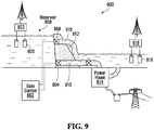
- a hydroelectric power generation company may use water level and flow data to decide whether to open a spillway in order to maintain the downstream water level above a minimum level necessary for fish survival. Without uncertainty quantification, entities such as the water agencies and the hydropower companies in the above examples would have to effectively make educated or even arbitrary guesses as to their own acceptable safety margins, but could suffer serious adverse consequences if those safety margins are either too large or too small.
- the adopted safety margin is larger than the uncertainty underlying the data, then the agency would tend to find itself unnecessarily evacuating residents from the flood plain on a routine basis even though no flooding was actually occurring, and likewise, the hydropower company could find itself unnecessarily opening the spillway and thereby wasting potential energy even though the downstream water level had not yet reached its minimum level.
- the adopted safety margin is smaller than the uncertainty underlying the environmental data, then the water agency may fail to evacuate even in situations where flooding does in fact occur, potentially resulting in a loss of human life, and likewise, the hydropower company may fail to open the spillway even in situations where the downstream water level drops below its minimum, potentially violating environmental compliance levels and adversely affecting aquatic life.
- Another disadvantage relates to the burdensome task of manually analyzing and qualitatively assessing the quality of environmental data for which quantified uncertainty information is unavailable.
- hydrologists typically analyze and grade (label) their data before they publicly release it, labeling each data point as "good” or "bad,” which may for example depend on whether the data point satisfies predefined expectations or constraints that the hydrologist associates with reliability of the data (e.g. a pH reading of 0 or 14 may be considered a "bad" data point for a river, on the assumption or expectation that the river is neither an extremely strong acid nor an extremely strong base.)
- Significant expenditures of time and effort are typically required to massage, grade and publish (release) data, and hydrologists are typically reluctant to publicly release their raw data until this laborious process has been completed.
- Such delays in public accessibility of data pose difficulties for those who require access to the data, for critical decision-making or for other reasons.
- the conventional rating curve is not a function of time, and will therefore begin to suffer increasing errors with the passage of time, until eventually hydrologists decide to shift the current rating curve or completely abandon it and build a new one from more recent data; the ongoing re-evaluation and re-building of rating curves are manual and often slow processes requiring expert judgment.
- Environmental data also presents the technical difficulty that it is difficult to accurately model. Unlike typical industrial processes, which are most often linear and stationary, the underlying physical processes for environmental data are typically non-linear, non-stationary (time-varying), complex and can well be described as chaotic processes. Both independent (input) and dependent (output) observations used for modeling are typically degraded by heteroscedastic noise. In fact, the dependent variable uncertainty may change with time and also with the magnitude of the independent variables. Even the continuous or periodic data used in real-time operation (after training) as input feed to the model, also tend to be degraded by non-stationary noise.
- one approach uses separate GPs, comprising one noise-free GP and a separate GP to model the input noise, but this approach merely effectively considers only input noise, and does not involve any separate consideration of the output noise associated with the dependent variable representing the physical environmental property being ultimately measured; rather, the resulting noise term consists solely of the propagated input noise.
- Another prior approach assumes no input noise and assumes output noise to depend upon input signal level, to model output signal heteroscedastic noise behavior, while yet another prior approach considers only input noise but fictitiously assumes the input and output noise variances to be identical, and thus both of these approaches fail to overcome the output noise difficulties mentioned above. More generally, existing GP solutions are not generally capable of simultaneous consideration of both the input noise associate with the independent variable(s) and the output noise associated with the dependent variable(s).
- Kersting, et al. disclose a GP approach to regression with input-dependent noise rates. This approach involves two GPs, one to model the noise-free output value and another to model the output noise variance. A most likely noise approach is used to approximate the posterior noise variance. This approach does not consider input noise associated with the input variable. ( Kersting, K., et al. "Most Likely Heteroscedastic Gaussian Process Regression", ICML '07, Proceedings of the 24th International Conference on Machine Learning, Corvalis, OR, USA, June 20-24, 2007, pages 393-400 .)
- Osborne et al. disclose an approach that uses GPs with an associated "fault bucket" to capture a priori uncharacterized faults, along with an approximate method for marginalizing the potential faultiness of all observations. The approach sums over only one fault variance, although the authors speculate that their approach could potentially be extended to sum over more than one fault variance in the future. ( Osborne et al.; "Prediction and Fault Detection of Environmental Signals with Uncharacterised Faults"; Proceedings of the 26th AAAI Conf. on Artificial Intelligence; 2012; p.
- U.S. Patent Application Publication No. US 2010/0174514 A1 to Melkumyan et al. discloses a system for large scale data modelling using Gaussian Processes (GP).
- the GP covariance function is a sparse covariance function that is smooth and diminishes to zero outside of a characteristic hyperparameter length.
- the modified covariance function allows large data sets to be modelled by Gaussian processes without having to arbitrarily reduce the size of the sampled data set. Only output noise is considered, as the input variables are geospatial co-ordinates with no associated noise.
- such embodiments tend to provide significant enhancements to environmental measurements, thereby allowing for significantly better decision-making, resulting in significantly greater operational efficiency of any system relying upon such measurements.
- a predictive probabilistic representation a respective range of possible values of the physical environmental property for each respective value of the at least one independent variable, with each such range of possible values reflecting both the input noise terms associated with the independent variable and the output noise terms associated with the physical environmental property, the uncertainty associated with the dependent observed physical environmental property has been reliably quantified in the form of its respective range of possible values for each respective value of the independent variable(s).
- this quantification of uncertainty is achieved without necessarily requiring any quantified uncertainty information for the independent observed physical environmental property.
- the system effectively generates "per-point" probabilistic representations of the dependent physical property; in other words, such an embodiment can generate a respective probability distribution function for each possible input data point (i.e. for each possible combination of independent variable values), and the probability distribution function for each such input point may be expressed in terms of moments of the probability distribution for the dependent variable, such as its expected value and variance.
- such embodiments tend to highlight the degree to which the variance itself varies over time and over the range of possible independent variable values: for example, the quantified variance tends to be larger near the extreme highs and extreme lows of the independent physical property, for which the available data is typically sparser.
- the above system can solve the problems that result from the conventional use of subjective manual grading and qualitative labeling of data points to represent the uncertainty on data, by instead associating a quantitative probabilistic representation with each input data point.
- such embodiments do not merely automate the previously manual task of labeling data, but rather, they replace that subjective manual task with an entirely different objective methodology which advantageously achieves repeatability and consistency: in contrast with conventional approaches whereby hydrologists used their own subjective insights and approaches to qualitatively grade and label their data, such embodiments instead employ an objective approach to express a quantitative measure of uncertainty, in the form of the predictive probabilistic representation for each input point.
- the grading of the data also tends to affect the resulting "rating curve" representing the functional relationship between the dependent and independent variable(s), since different hydrologists would tend to reach different conclusions as to which data points should be excluded from the rating curve model as outliers or "bad" data points.
- the conventional approach typically results in different hydrologists producing slightly different "rating curves" based on the same underlying data due to differences in the subjective approaches of the various hydrologists, such embodiments of the present disclosure avoid these difficulties and always arrive at the same rating curve if modeling the same underlying set of measurements.
- significant advantages also flow from the creation of the combined input and output noise levels matrix containing both input noise terms associated with the independent variable(s) and output noise terms associated with the physical environmental property, and more particularly from the resulting fact that the respective predictive probabilistic representations of the ranges of possible values of the physical environmental property reflect both the input noise terms and output noise terms.
- the embodiment solves a first technical problem with the operation of the computer processor that is being used to model and monitor the physical environmental property, by enabling a tractable solution to be obtained using a combination of native instructions from among the processor's predefined instruction set architecture.
- it has been found that such an embodiment tends to converge quickly in a small number of iterations, thereby providing a further technical advantage of improving the operational efficiency of the processor by reducing the number of floating-point operations that the processor must perform to arrive at a solution. This latter technical advantage is particularly useful for processing the large data sets that tend to typify environmental data.
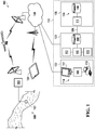
- an environmental monitoring system for monitoring a physical environmental property that has non-stationary heteroscedastic noise is shown generally at 100 in Figure 1 .
- the environmental monitoring system 100 includes a database 106 defined in a computer-readable storage medium shown generally at 104, configured to receive and store physical environmental measurement data.
- the physical environmental measurement data include measured values of a dependent variable which represents the physical environmental property, and at least one independent variable with which the physical environmental property is correlated.
- the system 100 further includes a processor 110 in communication with the storage medium 104, a communications interface 112 in communication with the processor 110, an output device 114 in communication with the processor 110, and a computer-readable medium 108 in communication with the processor 110.
- the computer-readable medium stores executable instructions that configure the processor to execute a method that includes the processor receiving the physical environmental measurement data, and the processor constructing a combined input and output noise levels matrix containing output noise terms associated with the physical environmental property and input noise terms associated with the at least one independent variable with which the physical environmental property is correlated.
- the processor constructs a main Gaussian Processes (GP) model that models the physical environmental property and its non-stationary heteroscedastic noise.
- the processor generates and co-operates with the output device 114 to perceptibly output a predictive probabilistic representation of the environmental property, using the main GP model.
- the predictive probabilistic representation includes a respective range of possible values of the physical environmental property for each respective value of the at least one independent variable, the range of possible values reflecting both the input noise terms associated with the independent variable and the output noise terms associated with the physical environmental property.
- the instructions stored in the computer-readable medium further configure the processor 110 to use a composite covariance function to generate an environmentally adapted covariance matrix corresponding to the values of the at least one independent variable, the composite covariance function including at least one stationary term comprising a rational quadratic term, and at least one non-stationary term.
- the processor 110 is further configured to receive a new value of the at least one independent variable through the communications interface 112, and to use the environmentally adapted covariance matrix and the physical environmental data to generate a predictive probabilistic representation of a range of possible values of the dependent observed physical environmental property corresponding to the new value of the at least one independent variable, the predictive probabilistic representation having moments including an expected value of the dependent variable and a variance.
- the processor 110 is further configured to cause the output device 114 to perceptibly output the predictive probabilistic representation.
- the environmental monitoring system 100 includes an environmental time series data management (ETSDM) system 102.
- the ETSDM system 102 includes an application server 103, a database server 105 and a client computer 107.
- the ETSDM system 102 includes a processor. More particularly, in this embodiment the ETSDM system 102 includes three processors 109, 110 and 111, of the client computer 107, the application server 103 and the database server 105, respectively.
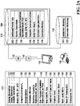
- the application server 103 includes the processor 110 in communication with a local computer-readable medium 108, with the communications interface 112, with the output device shown generally at 114, and with a memory device, which in this embodiment includes a Random Access Memory (RAM) 120.
- the computer-readable medium 108 stores instruction codes that configure the processor 110 to execute the various methods described herein, the instruction codes including an environment modelling routine 300 and an environment monitoring thread 400, discussed in greater detail below.
- the communications interface 112 enables the application server 103 to communicate with the other components of the system 100 via at least one communications network.
- the at least one communications network includes both a high-speed local area network (LAN) 195 by which the application server 103 communicates with the database server 105, and at least one wide area network (WAN) 196 by which the application server 103 communicates with the other components of the system 100.
- the communications interface 112 also allows the client computer 107 to communicate with the application server 103 via both an application programming interface (API) and a graphical user interface (GUI) executing on the client computer.
- API application programming interface
- GUI graphical user interface
- the client computer 107 includes the processor 109, which is configured to execute a client application (not shown) to enable the client computer 107 to communicate with the application server 103 and the database server 105 over the at least one wide area network shown generally at 196.
- the client computer 107 is configured to communicate with the application server 103 via both an application programming interface (API) and a graphical user interface (GUI) executing on the client computer 107.
- the output device 114 includes a video display device 117 and a printer 119 of the client computer 107.
- the database server 105 includes the database 106, along with the processor 111 which is configured to store and manage new environmental data under the direction of the application server 103.
- the at least one wide area network 196 includes the Internet, a cellular communications network and a satellite communications network, and accordingly, in this embodiment the communications interface 112 of the application server 103 includes a wired connection to the Internet as well as wireless connections to the cellular and satellite networks.
- the client computer 107 and database server 105 include similar communications interfaces (not shown).
- the above configuration is illustrative.
- the functions of the application server 103, the database server 105 and the client computer 107 can be otherwise divided, or can be combined in a single computing machine.
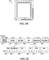
- the processor 110 of the application server 103 is shown in greater detail in Figures 2B and 2C .
- the processor 110 includes a hardware processor, specifically an Intel Xeon E5-2670 Dodeca-core (12-core) microprocessor, which is particularly well-suited to server applications.
- the processor 110 is connected to a motherboard of the application server 103 via a suitable multi-pin connector socket (not shown). More particularly, in this embodiment the processor 110 is connected via an LGA 2011 socket, although alternatively the Intel Xeon processor is also compatible with other sockets including LGA 2011-3, LGA 1150, LGA 1366, and PCI Express 2.0 and 3.0.
- the processor 110 is structurally configured with an internal microarchitecture which permits it to perform only a predefined set of basic or native operations in response to receiving corresponding instructions selected from a predefined instruction set architecture (ISA) of the processor.
- the instruction set architecture defines, among other things, the binary machine language OpCodes and native commands that the processor 110 is physically capable of executing.
- the instruction set architecture of the processor 110 includes an x86 instruction set architecture.
- the processor 110 is configured with a 64-bit implementation of the x86 instruction set architecture. Consequently, in this embodiment the processor 110 receives, via the LGA 2011 socket, binary machine-code instructions in accordance with the processor's x86 instruction set architecture.
- the format of a native instruction in accordance with the instruction set architecture of the processor 110 of the present embodiment is shown generally at 250.
- the instruction 250 can comprise instructions varying in length from 1 to 15 bytes.
- Each instruction 250 generally includes an OpCode field 252, a Mod R/M field 254, an SIB field 256, a displacement field 258 and an immediate field 260.
- the OpCode field 252 contains one or two bytes defining a native instruction OpCode to be executed.
- the Mod R/M field 254 contains a byte that specifies an addressing mode and instruction operand size; more particularly, the Mod R/M field 254 includes a Mod sub-field 262 specifying the x86 addressing mode, a Reg / OpCode sub-field 264 specifying the source or destination register, and an R/M sub-field 266 specifying either the operand in a single-operand instruction or the second operand in a two-operand instruction.
- the SIB field 256 contains a Scaled Indexed Byte for this purpose; more particularly, in this embodiment the SIB field 256 includes a Scale sub-field 268, an Index Scale Value sub-field 270 specifying an index register, and a Base sub-field 272 specifying a base register.
- the Displacement field 258 stores a memory address displacement for the instruction OpCode. If the instruction OpCode has an immediate operand then the Immediate field 260 stores immediate or constant data.
- the instruction 250 may further include one or more optional one-byte prefix fields 274, for storing one-byte instruction prefixes such as lock and repeat prefixes, bound prefixes, segment override prefixes, operand size override prefixes, and address-size override prefixes.
- one-byte instruction prefixes such as lock and repeat prefixes, bound prefixes, segment override prefixes, operand size override prefixes, and address-size override prefixes.
- the complete native instruction set for the 64-bit x86 instruction set architecture is available to the public from numerous sources.
- the complete native instruction set for the processor 110 is reproduced in, Intel® 64 and IA-32 Architectures Software Developer's Manual, Volume 2 (2A, 2B,2C & 2D): Instruction Set Reference, A-Z, Intel Order Number 325383-060US (Intel: September 2016 ).
- the environment modelling routine 300 and the environment monitoring thread 400 are stored in the computer-readable medium 108 in the form of executable machine codes forming instructions of the form shown in Figure 2C .
- the instruction codes of the various functional blocks of those routines including for example the processor receiving the physical environmental measurement data, constructing the combined input and output noise levels matrix, constructing the main GP model, and co-operating with the output device to generate and perceptibly output the predictive probabilistic representations, are stored in the computer-readable medium 108 in the form of respective sets of machine code instructions selected from the instruction set architecture.
- the system 100 further includes environmental measurement devices shown generally at 190, which in this embodiment include a plurality of sensors such as that shown at 192, an automated data logger and transmitter 193 and a plurality of discrete measurement remote uploading devices such as that shown at 194.
- environmental measurement devices shown generally at 190, which in this embodiment include a plurality of sensors such as that shown at 192, an automated data logger and transmitter 193 and a plurality of discrete measurement remote uploading devices such as that shown at 194.
- the ETSDM system 102 is configured to continuously or periodically receive new environmental sensor data inputs from the automated data logger and transmitter, each of the inputs including at least a new independent observed physical environmental property value along with its corresponding measurement time (time-value pair). More particularly, in this embodiment the independent observed physical environmental property value is stage (water level). Accordingly, in this embodiment the sensor 192 includes a water level sensor, disposed in a water channel such as a river or stream.
- the automated data logger and transmitter 193 is equipped with a communication link to allow it to continuously accumulate water level and time data and to periodically transmit the accumulated data to the ETSDM system 102 via the at least one wide area network 196.
- the at least one wide area network 196 includes the Internet, a cellular communications network and a satellite communications network
- the communications link of the automated data logger and transmitter 193 includes at least a wireless satellite communication link to the satellite network.
- any other suitable means of communication between the system 102 and the automated data logger and transmitter 193 may be substituted.
- the sensor 192 continuously measures the water channel's stage, i.e. the water level relative to a datum (fixed reference point), and communicates the measured (stage, time) value pairs to the automated data logger and transmitter 193, which accumulates corresponding pairs of stage values s and measurement time values t.
- each data point corresponding to each stage measurement taken by the sensor 192 is logged in the form of a time-value pair ( t, s ).
- the processor 110 of the application server 103 prepares the received data for storage in the database 106.
- such preparation includes validation, preprocessing and compression.
- a noise or error value ⁇ si for the i th value of the sensor 192 is known from the device firmware (which is not typically the case)
- the input of the i th value from the sensor 192 will also include the noise value ⁇ si in metadata transmitted by the automated data logger and transmitter 193.
- the noise element for continuous data is typically blank (or alternatively, may be fixed to the manufacturer's specification for a long range of time). Also, if additional independent variables are measured in a given embodiment, a new data set analogous to D C of equation (2) will be constructed and stored in the database 106.
- the automated data logger and transmitter 193 periodically transmits the accumulated sensor data points to the ETSDM system 102 via the wide area network 196, at a predetermined interval such as five minutes.
- the sensor 192 used to measure stage includes a pressure transducer that measures water pressure, and the sensor 192 includes firmware to convert the measured water pressure into a corresponding stage value.
- each data input transmitted to the system 102 may additionally include the measured water pressure value from which the corresponding stage value was calculated, which may also be stored in the database 106 in association with its corresponding stage and time values.
- additional values may be included in any embodiment in which the sensor measures the desired property indirectly, by measuring a different property and calculating the desired property.
- additional pressure values may be omitted for other stage sensor types that do not use pressure transducers, or more generally for sensors that directly measure their desired properties.
- the discrete measurement remote uploading device 194 generally allows a technician to enter various forms of discrete environmental measurements that the technician has just obtained from a field visit, and to upload those measurements into the database 106.
- the uploading device 194 may include a tablet computer running an uploading application, for example.
- the technician may record the discrete environmental measurements at the field site, either in paper field forms or electronically, and may upload them to the database 106 at a later time using the client computer 107 after the technician has returned from the field.
- the processor 110 of the application server 103 is configured to receive from the discrete measurement remote uploading device 194 or client computer 107, as the values of the at least one independent variable, observations of the at least one independent observed physical environmental property and corresponding times of the observations. More particularly, in this embodiment each such corresponding time value is received in the form of a time stamp accompanying its respective discrete observation of the independent observed physical environmental property. Likewise, in this embodiment, for each of the measurement times of the at least one independent observed physical environmental property, the processor 110 is configured to receive an observation of a dependent variable representing a dependent observed physical environmental property that is correlated with the independent observed property.
- the processor 110 is configured to receive discrete measurements of stage (water level) and accompanying time values as independent variables and discrete measurements of discharge (volumetric flow rate) as the dependent variable.
- the observations may include other physical environmental properties.
- the field technician in a typical field visit, could conceivably measure a broad range of observed properties, such as water level, measured discharge, water temperature, pH, dissolved oxygen, turbidity and air temperature, to name but a few examples.
- the field data include only measured stage (water level) and measured discharge q at measurement time t , so that each received data point is of the form ( t, s, q ) .
- the processor 110 of the application server 103 prepares the received data for storage in the database 106.
- such preparation includes validation, preprocessing and compression.
- each discrete data set may include further elements for further information.
- the discrete data set would include additional elements for such additional independent variables (and for their associated noise values if known, which is not typically the case).
- the processor separates the independent variables from the dependent variables, and generates and maintains a separate design matrix X DESIGN for the independent variables, a separate output vector y for the dependent variable, and a set of error vectors for all independent and dependent variables if they are available in the discrete observations store 204:
- any such vectors and matrices that are indicated to be stored in the database 106 are not stored in the form of defined matrices and vectors per se, but rather, for performance reasons, are typically stored as time series according to proprietary storage processes.
- vectors or more generally n-dimensional matrices may be defined and stored if desired.
- the acquisition, analysis and practical usage of environmental data pose special challenges not typically encountered in other technical fields.
- the main challenges in environmental data modelling come from four unique characteristics of both continuous and discrete observations: 1) the dynamic behaviour governed by underlying physical processes tends to be non-linear and non-stationary; 2) the uncertainty for measurements varies over time and over the range of measurements (heteroscedasticity); 3) a paucity or lack of observations at extreme conditions makes it difficult to accurately predict unobserved data at those conditions; and 4) some form of uncertainty measure (e.g., quality code, precision, accuracy, etc.) associated with individual observations may or may not be available, and if available, should preferably be used as input to the model.
- uncertainty measure e.g., quality code, precision, accuracy, etc.
- scalars are shown in lowercase normal (e.g. x 1 ), vectors in bold lowercase (e.g. x i ) and matrices in uppercase (e.g. K ) .
- the second term ⁇ xi T ⁇ x f ⁇ i represents how input uncertainty ⁇ xi T propagates into the output by multiplying by the gradient of f i and then linearly adding to the output uncertainty ⁇ yi .
- both input and output noise are Gaussians with mean 0 and variance that change over the input range: ⁇ yi ⁇ N 0 ⁇ yi 2 ⁇ x i ⁇ N 0 ⁇ x i
- f and e y we also model f and e y as Gaussian Processes (GP), or more particularly, as stochastic processes having multi-variate Gaussian distributions (see e.g. Rasmussen, C., & Williams, C., Gaussian Processes for Machine Learning (Boston: MIT Press, 2006 for more details).
- GP Gaussian Processes
- stochastic processes having multi-variate Gaussian distributions see e.g. Rasmussen, C., & Williams, C., Gaussian Processes for Machine Learning (Boston: MIT Press, 2006 for more details.
- standard GP solutions pre-dating the present application cannot be used.
- the probability of an observation y i for the final probabilistic model can be derived from equation (14): P y i
- f i , x i ⁇ N f i , ⁇ yi 2 + ⁇ x f ⁇ i T ⁇ x i ⁇ x f ⁇ i for i 1 , ... , n
- the present embodiment seeks to find the predictive distribution P ( f*
- the "posterior probability” represents the probability of a hypothesis H given observed evidence E, and is denoted P ( H
- the posterior probability may represent the probability of observing a discharge value f * given a new (stage, time) measurement x * and the previously observed discrete observations X .
- the "prior probability” represents the inherent likelihood of the hypothesis H, or more particularly the probability of hypothesis H before the evidence E is observed, and is denoted P ( H ) .
- the "likelihood” represents the compatibility of the observed evidence with the hypothesis, or more particularly, the probability of observing the evidence E given the hypothesis, and is denoted P ( E
- the "marginal likelihood” or “model evidence” is denoted P(E) and is the same for all possible hypotheses H, and can therefore be simply treated as a scaling factor z.
- the posterior probability equals the likelihood multiplied by the prior probability divided by the scaling factor, i.e. P H
- E P E
- H P H P E P E
- H P H dH P E
- the integral in the denominator is over high dimensional space and intractable, and different approximations are used.
- X , y P y
- X P y
- the predictive distribution for unobserved dependent variable f * at new independent variable vector x * can be calculated from sum (or marginalization) and product (Bayes) rules in probability theory: P f ⁇
- X , y , x ⁇ ⁇ P f ⁇
- the covariance function k RQ ( x, x' ) can be evaluated at any two given input points x and x' and the result represents the correlation (similarity/dissimilarity) between those two points.
- ⁇ f 2 , ⁇ , ⁇ are called hyperparameters that need to be estimated from observation.
- the present embodiment employs a novel composite covariance function combining at least one term that is stationary (only depends on differences x - x' ) and at least one term that is non-stationary (does not depend on differences x - x' ) .
- K ( X,X ) is the covariance matrix for all input observations with K ⁇ R n ⁇
- k(x*,x 1 )] and k(X,x*) k(x*,X) T ; and is the total variance for the noisy prediction.
- the first term is the model variance and the second term k y * is the variance associated with input and output uncertainties.
- log marginal likelihood can be derived as: logP y
- X ⁇ 1 2 y T K X X + K y ⁇ 1 y ⁇ 1 2 log K X X + K y ⁇ n 2 log 2 ⁇
- the present embodiment employs a novel iterative process, described in greater detail below in the "Operation" section in connection with blocks 310 to 340 of the environment modelling routine 300.
- the novel iterative process of the present embodiment may be briefly summarized as follows:
- the present inventor has found that convergence tends to occur quickly in just a few iterations of the above method with a typical number of stage-discharge discrete observations. In fact, even the first iteration tends to yield a good estimate of expected value for the predictive probabilistic distribution. In practice, independent and dependent noise levels for discrete observations are either not available or partially available, but almost always the range is given. Thus, the iterative process should be able to set constraints on parameter optimization for both performance and accuracy of the process, especially in respect of extremely sparse measurements.
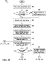
- an environment modelling routine is shown generally at 300 in Figures 2A and 3 .
- the environment modelling routine 300 configures the processor 110 of the application server 103 to model and monitor a physical environmental property that has non-stationary heteroscedastic noise, by first constructing a combined input and output noise levels matrix containing output noise terms associated with the physical environmental property and input noise terms associated with at least one independent variable with which the physical environmental property is correlated, then using the combined input and output noise levels matrix to construct a main Gaussian Processes (GP) model that models the physical environmental property and its non-stationary heteroscedastic noise, then co-operating with an output device to generate and perceptibly output a predictive probabilistic representation of the environmental property, using the main GP model.
- the predictive probabilistic representation includes a respective range of possible values of the physical environmental property for each respective value of the at least one independent variable, the range of possible values reflecting both the input noise terms associated with the independent variable and the output noise terms associated with the physical environmental
- the environment modelling routine 300 configures the processor 110 to construct the combined input and output noise levels matrix by constructing a simplified GP model representing the physical environmental property with stationary noise independent of inputs, then using the simplified GP model to construct a noise GP model representing noise levels associated with the environmental property.
- the environment modeling routine then configures the processor to use the simplified GP model and the noise GP model to construct the main GP model.
- the process carried out by the processor under the direction of the environment modelling routine 300 allows input uncertainty to be propagated without encountering analytically intractable differential equations, and allows the avoidance of assumptions about output noise that are inappropriate for environmental data, such as the typical GP assumption of fixed stationary noise.
- the execution of the environment modelling routine 300 solves a technical problem with the operation of the processor 110, making it possible to obtain a solution using a combination of native instructions from among the predefined instruction set architecture of the processor 110.
- the environment modelling routine 300 models stage-discharge relationships, with the independent input variables being time and the physical environmental property of stage (water level), and the dependent output variable being the physical environmental property of discharge (volumetric flow rate).
- the independent input variables being time and the physical environmental property of stage (water level)
- the dependent output variable being the physical environmental property of discharge (volumetric flow rate).
- x i t i s i T
- y i q i
- ⁇ yi ⁇ qi
- ⁇ xi 0 ⁇ si T
- ⁇ yi 2 ⁇ qi 2
- ⁇ x i 0 0 0 ⁇ si 2
- t is the time
- s stage and q is discharge.
- the environment modelling routine 300 directs the processor to define and solve for three Gaussian processes, namely, the Main GP model, the Simplified GP model and the Noise GP model discussed above. To assist in understanding the environment modelling routine 300, those three GPs are briefly summarized below.
- both the objective function used for optimization and its derivatives with respect to all hyperparameters should be constructed and given as a callback function to the optimizer.
- X 1 2 q T K X X + K q ⁇ 1 q + 1 2 log K X X + K q + n 2 log 2 ⁇
- ⁇ GPM ⁇ fRQ ⁇ RQ ⁇ 1 RQ ⁇ 2 RQ ⁇ EXP ⁇ 1 EXP ⁇ 2 EXP ⁇ 1 LIN ⁇ 2 LIN T
- This callback function reads hyperparameters and returns an objective function value F 0 and its gradient vector g .
- the optimization process calls this routine at each iteration.
- f i , x i ⁇ N f i ⁇ q 2 for i 1 , ... , n
- the callback function for optimization will be the same as for the Main GP (GPM) above, with the exceptions that the hyperparameter vector ⁇ GP1 will include the additional hyperparameter ⁇ q , and that the callback function for GP1 can be successfully executed using only stage and discharge observations, without having to obtain estimates of the average of the latent function or output noise.
- the input is x i similar to GPM and GP1 but output is the logarithm of noise levels.
- the Bayesian prior on function e for the Noise GP model (GP2) is governed by a different covariance function than that which governs the main and simplified GP models GPM and GP1, reflecting the fact that GP2 is for modelling the noise levels rather than the physical environmental property data.
- the predictive distribution for e process can be calculated from:
- empirical estimates for the e i values calculated from the results of GP1 will be used to construct the training data for this e process (i.e. for the Noise GP model GP2).
- the environment modelling routine 300 begins with a first block 302 of codes, which directs the processor 110 to pre-process and partition the environmental data. More particularly, the environmental data to be pre-processed and partitioned includes the discrete data set D D stored in the discrete observations store 204 of the database 106, as discussed above in connection with equations (3) and (4).
- block 302 directs the processor 110 to communicate with the database server 105 to read the contents of the discrete observations store 204 and to calculate the logarithm (base e ) of both the independent and dependent physical environmental properties, which in this embodiment are stage and discharge.
- block 302 then directs the processor 110 to normalize the stage and discharge values.
- Block 302 first directs the processor 110 to calculate the mean m s and standard deviation ⁇ s of the n stage-log values S L , and to likewise calculate the mean m q and standard deviation ⁇ q of the n discharge-log values q L .
- Block 302 directs the processor 110 to temporarily store the resulting normalized stage and discharge values S Ni and q Ni in a cache memory portion (not shown) of the RAM 120.
- block 302 then directs the processor 110 to partition the normalized observations.
- the present embodiment uses only a portion of the available discrete observations to train the model; a further portion is used for testing, as described below.
- block 302 prompts a user to either approve a default partitioning of the data, or to manually enter different partition boundaries to thereby select a specific portion of the discrete observations for training the model. More particularly, in this embodiment the default partitioning uses a random selection of 70% of the discrete observations for training, and uses the remaining 30% for testing, unless the user specifies which particular observations or cluster of observations should be used in which partition.
- block 302 directs the processor 110 to partition the discrete observations into training observations and testing observations.
- Block 302 directs the processor 110 to copy the training portion and testing portion of the normalized discrete observations to, respectively, a training observations store 122 and a testing observations store 126 in the RAM 120.
- block 304 then directs the processor 110 to determine whether uncertainty information is available for any of the training data stored in the training observations store 122. More particularly, block 304 directs the processor 110 to determine whether the discrete observations store 204 in the database 106 contains either non-zero stage error values ⁇ si or non-zero discharge error values ⁇ qi for all time-index values corresponding to those of the training data.
- block 306 directs the processor 110 to apply a constraint to the environmental model using the uncertainty information. More particularly, in this embodiment if input noise information is available for the discrete observations of the independent physical environmental property (in this case, stage), then block 306 directs the processor 110 to set an input noise flag active, and likewise if output noise information is available for the discrete observations of the dependent physical environmental property (in this case, discharge), then block 306 directs the processor to set an output noise flag (not shown) active, to indicate that input and/or output uncertainty information is available, respectively. Block 306 directs the processor to copy the available input and output uncertainty information to an input noise portion and an output noise portion, respectively, of an available uncertainty store 128 in the RAM 120.
- block 306 directs the processor 110 to constrain the model by setting the input noise flag active and by setting each of the noise values ⁇ s1 ... ⁇ sn in equation (42) equal to ⁇ s rather than including ⁇ s1 ... ⁇ sn within equation (48) as additional hyperparameters to be optimized according to the steps described below.
- Block 306 directs the processor to store the input noise values ⁇ si in an input noise portion of the available uncertainty store 128 in the RAM 120.
- block 308 directs the processor 110 to select a composite covariance function for the Main GP (GPM), which will also be used for the Simplified GP (GP1). (However, as discussed below in connection with block 318, a different covariance function is used for the Noise GP, GP2.)
- GPM Main GP
- GP1 Simplified GP
- the construction or selection of a suitable covariance function tends to be a complex process requiring significant expertise and ingenuity, in order to select a covariance function having a general form that is sufficiently close to the true form to allow the hyperparameters to be optimized in a feasible number of iterations.
- the present embodiment avoids the need for users to possess such expertise and ingenuity, by configuring the processor 110 to automatically select a composite covariance function from among a plurality of predefined composite covariance functions stored in a composite covariance functions store 210 in the database 106, in which each of the predefined composite covariance functions corresponds to a particular respective observed physical environmental property that the system 102 is designed to model.
- the predefined composite covariance function corresponding to stage-discharge data may differ from the predefined composite covariance function for turbidity data.
- the automatic selection of an appropriate predefined composite covariance function improves the repeatability and consistency of rating curves, in comparison to conventional approaches in which different hydrologists would often select different covariance functions and arrive at slightly different rating curves.
- block 308 directs the processor 110 to automatically select, from among the plurality of predefined composite covariance functions in the composite covariance functions store 210, a composite covariance function that the processor will use to generate an environmentally adapted covariance matrix corresponding to the values of the at least one independent variable, as discussed in greater detail below in connection with block 332.
- the automatically selected composite covariance function includes at least one stationary term including a rational quadratic term, and at least one non-stationary term. More particularly still, in this embodiment the at least one non-stationary term includes a linear term, and further includes an exponential term.
- the physical environmental data includes hydrological data relating to a waterway
- the at least one independent variable includes stage and time (stage representing a measured water level of the waterway, and the time at which the water level was measured)
- the dependent variable includes a discharge or flow rate of the waterway at the time.
- the exponential term provides a good initial form for modelling the water channel data
- the linear term provides improved results for extreme high and extreme low stage values
- the rational quadratic term advantageously provides the flexibility to have breakpoints across the channel and to model possible nonlinear changes in the time dimension that may result from environmental changes (the rational quadratic term can model nonlinearity in both the stage and time dimensions).
- Block 308 directs the processor 110 to store the selected composite covariance function in a composite covariance function store 130 in the RAM 120.
- ⁇ ⁇ fRQ ⁇ RQ ⁇ 1 RQ ⁇ 2 RQ ⁇ EXP ⁇ 1 EXP ⁇ 2 EXP ⁇ 1 LIN ⁇ 2 LIN T
- block 308 directs the processor to check whether the input noise flag that was set at block 306 is active to indicate available input noise, and if not, block 308 directs the processor to add the input noise terms ⁇ s1 ... ⁇ sn to the hyperparameter vector of equation (72) for optimization.
- unknown input noise can be determined from a separate "single sensor" execution of the environment modelling routine, as discussed under “Alternatives” below.
- output noise terms ⁇ yi 2 (or ⁇ qi 2 in this embodiment) are estimated differently as described below at blocks 320 and 321.
- k from equation (65) above corresponds to the noise-free or latent function f(x) from equation (14) above.
- the additional noise terms of equation (14) correspond to independent and dependent noise terms shown in the K y matrix.
- composite covariance functions may be stored and selected for different types of environmental data.
- a composite covariance function relating to index velocity data may omit an exponential term and provide only a linear non-stationary term in combination with a stationary rational quadratic term in both time and index velocity input dimensions.
- block 310 directs the processor 110 to initialize the hyperparameters for the three defined Gaussian processes. To achieve this, block 310 first directs the processor 110 to initialize the hyperparameters shown in equation (72) above for the Main GP (GPM). Block 310 first directs the processor 110 to determine whether optimized hyperparameters for the selected composite covariance function and for the discrete observations have been previously stored in an optimized hyperparameters store 214 in the database 106.
- block 310 directs the processor 110 to use the previously optimized hyperparameters as the initial values of the hyperparameters, and to store these initial values in a Main GP hyperparameters portion of a hyperparameters store 132 in the RAM 120. If not, then in the present embodiment, block 310 directs the processor to set the initial value of all hyperparameters for GPM to 1.
- block 310 also directs the processor 110 to initialize the hyperparameters for the Noise GP model GP2.
- block 310 directs the processor 110 to determine whether optimized hyperparameters for the noise GP model GP2 have been previously stored in an optimized hyperparameters store 214 in the database 106, and if so, to use the previously optimized hyperparameters as the initial values of the GP2 hyperparameters, and to store these initial values in a Noise GP hyperparameters portion of the hyperparameters store 132 in the RAM 120.
- block 310 directs the processor to set the initial value equal to one, for each of the hyperparameters of the hyperparameter vector of equation (55) above, and to store the initialized hyperparameter values in the Noise GP hyperparameters portion of the hyperparameters store 132 in the RAM 120.
- block 312 directs the processor 110 to estimate hyperparameters of the Simplified GP model GP1.
- block 312 directs the processor to optimize the hyperparameters by executing a callback function to a standard optimization routine, such as the fminunc function in the Matlab (from Mathworks) optimization toolbox, for example.
- the optimal hyperparameters for GP1 are those that maximize its log marginal likelihood, or equivalently, that minimize its negative log marginal likelihood.
- the callback function may be represented by the following pseudo-code:
- the callback function executed at block 312 for the Simplified GP model GP1 returns the requested value of the objective function F 0 and its gradient vector g , for each iteration.
- the callback function continues to iteratively adjust and test hyperparameter values, producing new values of F 0 and its gradient vector g , until F 0 converges to a minimum.
- the callback function returns the co-ordinates in hyperparameter space of the located minimum, thereby returning optimized values of all of the hyperparameters of the augmented hyperparameter vector ⁇ GP 1 of equation (51) above.
- Block 312 directs the processor 110 to store the optimized hyperparameters in a Simplified GP portion of the hyperparameters store 132 in the RAM 120.
- block 312 also directs the processor 110 to transmit the optimized hyperparameters to the database server 105, for storage in a Simplified GP portion of an optimized hyperparameters store 214 in the database 106.
- block 314 then directs the processor 110 to generate an average or expected value of the Simplified GP model GP1, for each of a plurality of training points.
- the training points are the points in independent variable space for which partitioned discrete observations are stored in the training observations store 122 in the RAM 120, following execution of block 302 above.
- block 314 Given training data X and q stored in the training observations store 122 at block 302 above, and the optimized hyperparameters ⁇ GP1 of the Simplified GP model GP1 stored in the Simplified GP portion of the hyperparameters store 132 at block 312 above, block 314 directs the processor 110 to calculate an expected or average value from equation (39) above, for each training data point, as follows: where x i are training inputs and f i is the expected or estimated mean value for discharge q at training point x i . Block 314 directs the processor 110 to store the resulting expected values in a Simplified GP expected values store 150 in the RAM 120.
- block 315 then directs the processor 110 to determine whether output noise (discharge error) information for the training data set is available and was stored in the available uncertainty store 128, as discussed above at blocks 304-306, by checking whether the output noise flag was set active at block 306. If so, then block 321 directs the processor to read the output noise values ⁇ qi stored in the output noise portion of the available uncertainty store 128, and to store them as output noise estimates in an estimated output noise store 156 in the RAM 120, and the processor is then directed to block 322 below.
- output noise discharge error
- the processor is directed by blocks 316 to 320 below to generate estimates of output noise levels for the Main GP model GPM, using the Noise GP model GP2.
- block 316 directs the processor 110 to generate an empirical error term of the Simplified GP model GP1 for at least some of the plurality of training points. More particularly, block 316 directs the processor to randomly select at least m different samples q ⁇ i j (preferably m>50) of the expected or estimated discharge values that were stored in the simplified GP expected values store 150 at block 314 above (labelled as estimates of the expected value or average f i in connection with block 314).
- Block 316 directs the processor 110 to store the resulting training data set in a noise GP training data store 154 in the RAM 120.
- block 318 then directs the processor 110 to estimate hyperparameters of the Noise GP model GP2, in a manner similar to the hyperparameter optimization for the Simplified GP model GP1 above at block 312. More particularly, in this embodiment block 318 directs the processor 110 to pass the training data set stored in the noise GP training data store 154 (generated at Block 316 using equation (77)), along with the initialized values of the hyperparameters stored in the Noise GP hyperparameters portion of the hyperparameters store 132 (generated at block 310), to a callback function of Matlab (or any other suitable standard optimization package).
- block 318 may be represented by the following illustrative pseudo-code: where X, e comprise the training data set D generated at block 316 above.
- the callback function executed at block 318 for the Noise GP model GP2 returns the requested value F 0 of the objective function F from equation (58) and its gradient vector g from equation (59), for each iteration.
- Block 318 directs the processor 110 to store the optimized hyperparameters in a Noise GP portion of the hyperparameters store 132 in the RAM 120. In this embodiment, block 318 also directs the processor 110 to transmit the optimized hyperparameters to the database server 105, for storage in a Noise GP portion of an optimized hyperparameters store 214 in the database 106.
- block 320 then directs the processor 110 to generate output noise levels for the Main GP model GPM using the Noise GP model GP2.
- block 320 first directs the processor 110 to use the training data set from the noise GP training data store 154 and the optimized hyperparameters ⁇ GP2 from the Noise GP portion of the hyperparameters store 132, in conjunction with equation (56) above, to calculate an expected value or predicted mean: where x i are training inputs.
- Block 320 directs the processor to use equations (56), (78) and (79) above to generate the above estimates of output noise levels, and to store them in the estimated output noise store 156 in the RAM 120.
- block 322 then directs the processor 110 to construct a combined input and output noise levels matrix for the Main GP model (GPM) using the generated output noise levels from block 320 above. More particularly, block 322 directs the processor to use the expected values f i of the Simplified GP model GP1 that were calculated at block 314 and stored in the simplified GP expected values store 150, along with their corresponding stage values s from the training observations store 122, as well as the estimated output noise levels ⁇ qi that were calculated at block 320 and stored in the estimated output noise store 156, to construct a combined input and output noise levels matrix K q given by equation (42) above. With respect to the input noise term ⁇ s1 ...
- Block 322 directs the processor 110 to store the combined input and output noise levels matrix in a noise levels matrix store 158 in the RAM 120.
- block 324 then directs the processor 110 to estimate the hyperparameters of the Main GP model (GPM), using the combined input and output noise levels matrix generated at block 322 above.
- block 324 first directs the processor 110 to re-initialize the hyperparameters for the Main GP model GPM, by setting the hyperparameter values ⁇ GPM of the Main GP portion of the hyperparameters store 132 equal to the already optimized hyperparameters ⁇ GP1 stored in the Simplified GP portion of the hyperparameters store 132.
- Block 324 then directs the processor to pass the re-initialized hyperparameters to a standard optimization callback function, along with the training data X and q from the training observations store 122 and the combined input and output noise levels matrix K q from the noise levels matrix store 158.
- the callback function executed by the processor at block 324 may be represented by the following illustrative pseudo-code:
- the callback function executed at block 324 for the Main GP model GPM returns the requested value F 0 of the objective function F from equation (46) and its gradient vector g from equation (47), for each iteration.
- Block 324 directs the processor 110 to store the optimized hyperparameters in a Main GP portion of the hyperparameters store 132 in the RAM 120. In this embodiment, block 324 also directs the processor 110 to transmit the optimized hyperparameters to the database server 105, for storage in a Main GP portion of an optimized hyperparameters store 214 in the database 106.
- block 328 directs the processor 110 to determine whether a predefined maximum number of iterations has been reached, suggesting that the total objective function is oscillating rather than converging. If so, the environment modelling routine 300 is ended; optionally, if desired, block 328 may prompt a user to adjust one or more parameters of the environment modelling routine 300, such as decreasing the step sizes of each hyperparameter iteration for example, and may further prompt the user to re-execute the environment modelling routine 300 with the adjusted parameters.
- block 330 directs the processor to overwrite the contents of the convergence test store 160 with the current sum of objective functions F total .
- block 332 directs the processor 110 to use a composite covariance function to generate an environmentally adapted covariance matrix corresponding to the values of the at least one independent variable, the composite covariance function including at least one stationary term including a rational quadratic term, and at least one non-stationary term. More particularly, in this embodiment block 332 directs the processor to generate the covariance matrix K(X, X) for the Main GP model GPM, using the definition of the covariance matrix from equation (43), the composite covariance function defined by equations (65) to (68) that was selected at block 308 above, and the optimized hyperparameters ⁇ GPM that were obtained at block 324 and stored in the Main GP portion of the hyperparameters store 132.
- block 332 directs the processor 110 to store the environmentally adapted covariance matrix in a Main GP portion of a covariance matrices store 136, and also directs the processor 110 to transmit the environmentally adapted covariance matrix to the database server 105, for storage in a covariance matrices store 218 in the database 106.
- block 336 then directs the processor 110 to calculate predictive probabilistic representation values for the Main GP model GPM. More particularly, in this embodiment block 336 directs the processor to generate a predictive probabilistic representation of a range of possible values of the dependent observed physical environmental property (in this case, discharge), for each of a plurality of independent variable (stage, time) data points.
- block 336 directs the processor to use the composite covariance function of equations (65) to (68) with the optimized hyperparameters ⁇ GPM that were stored in the Main GP portion of the hyperparameters store 132, and the corresponding covariance matrix stored in the Main GP portion of the covariance matrices store 136, to solve for the expected value or average given by equation (39) and the variance given by equation (41), for each input x i of each discrete observation stored in the training observations store 122.
- Block 336 directs the processor to store the resulting expected value and variance for each training data input x i in a predictive probabilistic representation-per-point store 140.
- Block 336 also directs the processor 110 to transmit the resulting expected value and variance for each training point to the database server 105, for storage in a continuous derived probabilistic representation per point store 216 in the database 106.
- Block 338 directs the processor to store the results of the test in a model test results store 209 in the database 106, in association with the contents of the optimized hyperparameters store 214 and of the covariance matrices store 218 that correspond to the current model being tested.
- the predictive probability distribution can be used to generate a dependent variable output (discharge), in the form of a probability distribution represented by an expected value and a variance from equations (25), (26) and (27), for any further independent variable input vector (stage, time), irrespective of whether the further input vector is new or old sensor data for which no output is available, or new or old input vectors for which an output is available, as discussed below.
- block 340 then directs the processor 110 to co-operate with the output device 114 to perceptibly output predictive probabilistic representations of a range of possible values of the dependent observed physical environmental property (discharge), each such representation corresponding to a respective observation of the independent variables (stage and time). More particularly, in this embodiment the processor co-operates with the video display device 117 to display the predictive probabilistic representation.
- the predictive probabilistic representation includes, for each respective value of the at least one independent variable, an expected value of the physical environmental property and an associated variance.
- block 340 directs the processor 110 to communicate with the client computer 107 via the communications interface 112, to cause the video display device 117 to display the predictive probability distributions generated at block 336 for the testing observations from the testing observations store 126.
- Block 340 directs the processor 110 to post-process the probability distributions, or more particularly their expected values and variances, to reverse the effects of the pre-processing that was carried out at block 302, effectively de-normalizing and taking the exponentials of the probability distributions, to thereby reverse the effects of equations (61) to (64) above.
- Block 340 directs the processor 110 to store the post-processed probability distributions in a post-processed probability distributions store 148 in the RAM 120.
- Block 340 then directs the processor 110 to communicate with the client computer 107 to cause the video display device 117 to generate a visual display of the probabilistic representations of the dependent environmental property.
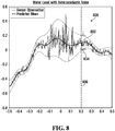
- block 340 advantageously directs the processor to instead co-operate with the video display device 117 to display an expected value curve 504 in conjunction with a heteroscedastic combined variance band 506 that reflects both the input noise terms and the output noise terms of the combined input and output noise levels matrix.
- the expected value curve 504 includes the expected value of the physical environmental property, and the heteroscedastic combined variance band extends above and below the expected value curve 504 and has a variable height 508 for a particular expected value that is proportional to the associated variance for the particular expected value.
- the perceptibly displayed predictive probabilistic representation comprising the expected value curve 504 and combined variance band 506 immediately inform a decision-maker or other user of the system 100 of the errors associated with the expected value curve 504, so that the decision-maker can consider not only whether the expected value curve 504 crosses a critical threshold, but more significantly whether the combined variance band 506 crosses the critical threshold.
- block 340 also prompts the user as to whether to print the probabilistic rating representations displayed above. If so, block 340 directs the processor 110 to co-operate with the printer 119 to print the predictive probabilistic representations, by communicating with the client computer 107 to cause the printer 119 to generate a tangible printout (in this embodiment including ink on paper) representing the predictive probabilistic representations.
- a tangible printout in this embodiment including ink on paper
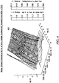
- block 340 In addition to perceptibly outputting the predictive probabilistic representations for the testing discrete observations, in this embodiment block 340 also prompts the user to select other types of perceptible output options. For example, referring to Figures 3 and 6 , in this embodiment block 340 prompts the user as to whether to generate and perceptibly output a rating hypersurface comprising an expected value of the dependent observed physical environmental property for each combination of values of the at least one independent variable. If so, then in this embodiment block 340 directs the processor 110 to co-operate with the output device 114 to generate and perceptibly output a time-varying rating surface or hypersurface reflecting the evolution over time of a relationship between the dependent observed physical environmental property and the at least one independent observed physical environmental property.
- block 340 directs the processor 110 to co-operate with the video display device 117 to generate and perceptibly output a three-dimensional rating surface 602 shown in Figure 6 comprising an expected value of the discharge or flow rate for each combination of values of stage and time.
- the variance may also be shown as a variable vertical thickness of the expected value surface, but is not shown in Figure 6 to avoid obscuring the expected value surface.
- block 340 presents the user with the option of repeating the functions of block 336 above to construct appropriate probability distributions for other possible input points, thereby enabling the perceptible output of the corresponding predictive probabilistic rating representations.
- block 342 then directs the processor to either continue executing an environment monitoring thread 400 stored in the database 106 or to begin executing it if it is not already in progress, and the environment modelling routine 300 is then ended.
- the environment monitoring thread 400 configures the processor 110 to receive physical environmental measurement data including measured values of a dependent variable which represents the physical environmental property, and of at least one independent variable with which the physical environmental property is correlated.
- the environment monitoring thread either generates and perceptibly outputs a new predictive probabilistic representation, or regenerates the combined input and output noise levels matrix and the main GP model to take into account the new field data, as discussed in greater detail below.
- the environment monitoring thread 400 begins with a first block 402 of codes, which directs the processor 110 to determine whether new continuous / periodic data, including a new value of the at least one independent variable, has been received by the processor 110. More particularly, in this embodiment block 402 enables the processor 110 to continuously or periodically receive new values of the at least one independent variable, the new values including new environmental sensor data inputs, each of the sensor data inputs including at least a new stage value and a new measurement time value, but excluding any observation of the dependent variable (discharge), which is to be calculated by the system 100.
- the processor 110 receives such continuous / periodic data in the form of measurement signals transmitted by one or more of the remote sensors 192 disposed in the environment or by a remote data logger disposed in proximity to the remote sensors. More particularly, in this embodiment the remote sensors 192 transmit measurement signals encoding each of their respective measurements to the automated data logger and transmitter 193, which accumulates and periodically re-transmits the measurement signals to the processor 110.
- the measurement signals include at least time and stage values representing a water level of a waterway as measured by one or more stage sensors such as the sensor 192 disposed in the waterway.
- block 404 Upon receipt of new continuous / periodic data, block 404 directs the processor 110 to store the new data in the continuous / periodic data store 202 in the database 106, and to pre-process the new data in the manner described above in connection with block 302 of the environment modelling routine 300. In this embodiment, block 404 directs the processor 110 to store both the raw data and the pre-processed data in the continuous / periodic data store 202 in the database 106, and to copy the pre-processed data to a new continuous / periodic data store 144 in the RAM 120.
- block 406 then directs the processor 110 to use the main GP model to generate and perceptibly output a predictive probabilistic representation of a range of possible values of the dependent observed physical environmental property corresponding to the new value of the at least one independent variable, the predictive probabilistic representation having moments including an expected value of the dependent variable and a variance, in the manner described above in connection with the environment modelling routine 300. More particularly, in this embodiment block 406 directs the processor 110 to co-operate with the output device 114 to generate and perceptibly output a new expected flow rate (discharge) value and a new flow rate variance value corresponding to the new stage and new measurement time values.
- block 406 first directs the processor to load into the hyperparameters store 132, the most recently optimized hyperparameters from the optimized hyperparameters store 214 in the database 106, for the model to which the incoming data corresponds. Block 406 then directs the processor to construct all covariance matrices and the K q and k q terms in equations (23) and (24), and to use equations (25) and (27) to generate an expected value and variance for each new data point in the new continuous / periodic data store 144, in a manner similar to block 336 above.
- Block 408 then directs the processor 110 to post-process the resulting predictive probability distributions to reverse the effect of pre-processing at block 404, and block 410 then directs the processor 110 to communicate with the client computer 107 to cause the video display device 117 to perceptibly output a probabilistic rating representation comprising the expected value curve and the variance band of the predictive probability distributions ( i.e. and ), in a manner similar to that shown in Figure 5B and discussed above in connection with the environment modelling routine 300.
- block 412 then directs the processor 110 to determine whether it has received new field data including at least one new discrete field observation of the at least one independent variable and the dependent variable, from the discrete measurement remote uploading device 194 or from the client computer 107. If so, block 414 directs the processor 110 to append the new discrete data to the discrete observations store 204 in the database 106, and then directs the processor 110 to re-execute the environment modelling routine 300 in its entirety, thereby re-generating the environmentally adapted covariance matrix, the combined input and output noise levels matrix, and ultimately the main GP model, to take into account the new field data. Alternatively, if discrete data are received more frequently than a user wishes to re-optimize the hyperparameters, block 414 may impose a predefined or user-defined minimum interval between successive re-optimizations.
- the iterative optimization is performed by optimizing hyperparameters for GPM (which starts from GP1) and GP2 separately with standard GP optimization and using the main optimization convergence criteria (objective function) composed of sum of the marginal likelihood functions for both GPs as described in connection with step 9 (block 326) to end the iterative loop.
- the composite objective function for both GPs is used at step 9 to adjust all hyperparameters for GPM and GP2 at each iteration.
- the method of the environment modelling routine 300 described above tends to converge with high accuracy, this alternative embodiment may tend to achieve convergence faster for some large data sets.
- the optimization method of the environment modelling routine 300 has tended to outperform the alternative method in both performance and accuracy and has therefore been presented as the main embodiment above.
- Figures 7A and 7B show the application of similar techniques to water quality data, specifically turbidity data. More generally, the techniques described herein may be applicable to any environmental property for which discrete observations are obtained, such as e.coli levels, phosphorus levels, etc.
- a composite covariance function comprising a rational quadratic stationary term and a non-stationary term may be employed, although the precise form of the non-stationary and stationary terms may differ from those employed for stage-discharge data.
- the composite covariance function for an illustrative water quality embodiment may include a rational quadratic term as the stationary term in combination with a linear term as the non-stationary term.
- the rational quadratic term allows nonlinear aspects of both time and other independent variable(s) to be accurately modeled, while the linear term improves accuracy as the model extends into extreme high and low values of the independent variables for which few or no observations may be available.
- the methods of the present disclosure may also be applied in different ways to hydrometric data.
- stage water level
- the independent variable may comprise a pressure transducer measurement from a sensor that calculates stage measurements from observed pressure measurements.
- the independent variables may include time, and may further include one to many index velocity measurements from a plurality of Acoustic Doppler Velocity Meters (ADVMs), either for individual cells or cell average signals.
- ADVMs Acoustic Doppler Velocity Meters
- the independent variables may further include stage (water level).
- the dependent variable may be discharge, or may be overall mean velocity. Generally, such use of discharge as a dependent variable correlated with index velocity as an independent variable is not believed to be known in the art.
- Such embodiments tend to provide more accurate estimates for discharge when directly modeled with index velocity, or with both index velocity and stage, as predictors (independent variables).
- such embodiments tend to simplify relevant hydro acoustic methodologies and protocols. For example, a conventional cross section survey to measure area (to multiply it by mean velocity to get discharge) is no longer necessary in such embodiments, and the elimination of this step tends to reduce the uncertainty associated with the final estimate of discharge.
- the relationship between the dependent and independent variables tends to be close to linear (in linear space, without logarithmic pre-processing) but changing over time.
- the composite covariance function preferably includes both a non-stationary linear term, which assists in modeling extreme high and low values of the independent variables, and a stationary rational quadratic term, which assists in modeling nonlinear aspects of both time and other independent variable(s), as discussed above.
- the present embodiment also advantageously presents the user with a gap-filling option.
- any such gaps in the independent physical environmental property data can be filled by executing the environment modelling routine 300 above in only a slightly different manner, by treating what was previously considered to be the "independent" physical environmental property as if it were the dependent or output property, and treating time as the sole independent variable.
- the only independent variable is time steps and the dependent variable is the actual observed property values so there is no independent variable noise.
- step 3 in the iterative process (block 314 above) can be skipped and no derivative calculation is needed. Otherwise, the environment modelling routine 300 may be executed as described above, to yield expected values and variances for the missing data, and to cause the display device to perceptibly display them.
- block 320 may nevertheless generate probability distributions, comprising an expected value 704 and variance 706 for each possible input in a given range.
- Figures 7A-7C depict turbidity sensor data rather than discharge, but the advantageous effects are similar for other types of environmental sensor data.
- This process can be run online when new continuous observations are received.
- This type of model is referred to as a single sensor data model since there is no predictor except time.
- stage water level
- environment modelling routine 300 may otherwise be applied as described above.
- a predictive probabilistic representation of stage water level is shown generally at 800 in Figure 8 , and includes an expected stage value 802 and a variance 804 representing noise associated with each such stage value.
- Figure 8 in fact shows a predictive probabilistic representation of continuous / periodic sensor data as generated above at blocks 406 to 410 with heteroscedastic input noise represented by the variance 804, but a predictive probabilistic representation of discrete field observations of stage would have the same general form as Figure 8 .
- an additional block 305 of codes directs the processor 110 to generate input noise values ⁇ s1 ...
- block 305 directs the processor 110 to store the generated stage noise values ⁇ s1 ... ⁇ sn in the input noise portion of the available uncertainty store 128 in the RAM 120.
- a flow control system for a hydroelectric power generation station having a spillway is shown generally at 900 in Figure 9 .
- the flow control system 900 includes a gate control system 902 for controlling a power generation gate 904 and a spillway gate 906, which in this embodiment include electro-mechanical gates.
- the power generation gate 904 when opened, allows water to flow from a reservoir 908 through a power house conduit 910 defined through a dam 912, and then through a power house 914 to drive a turbine and generator, to thereby generate electricity.
- the gate control system 902 includes an environment monitoring system similar to the system 100 shown in Figure 1 , in communication with electromechanical actuators (not shown) to enable the processor of the gate control system 902 to open and close the power generation gate 904 and the spillway gate 906.
- the gate control system 902 includes downstream stage sensors such as that shown at 916 for measuring the water level downstream of the dam 912, and upstream stage sensors such as that shown at 920 for measuring the water level in the reservoir 908 upstream of the dam 912, in communication with a processor of the gate control system 902 via respective automated data logger/transmitters 918 and 922.
- constraints such as a maximum or minimum
- two or more of these and other similar constraints apply.
- constraints such as a maximum or minimum
- the spillway gate 906 would be frequently opening unnecessarily, because the difference between the measured downstream water level and the minimum threshold level would frequently be less than the massive safety margin, even though the true values of the downstream stage would not actually fall below the minimum threshold.
- a competing desire to minimize the opening of the spillway gate, in order to minimize such energy loss.
- the processor of the gate control system 902 executes the environment modelling routine 300 and the environment monitoring thread 400, wherein the physical environmental property represented by the dependent variable comprises stage, wherein the stage represents a measured water level of the waterway.
- the processor of the gate control system then receives a new measured stage value, and uses the main GP model to generate and perceptibly output a predictive probabilistic representation of a range of possible stage values corresponding to the new measured stage value.
- the gate control system processor then causes the spillway to be opened if the range of possible stage values includes any value below a predefined minimum stage threshold value, regardless of whether the new measured stage value is below the threshold value.
- the decision to open the spillway gate 906 may be based on other factors, including upstream reservoir stage, downstream or upstream discharge (flow rates), or combinations thereof, for example.
- the processor of the gate control system 902 executes the environment modelling routine 300 with discharge (flow rate) as the dependent variable and with stage and time as the independent variables.
- the processor of the gate control system 902 would thus model and represent the discharge with an expected value curve 504 in conjunction with a heteroscedastic combined variance band 506 as shown in Figure 5B and as discussed earlier herein.
- the processor As new current measurements of stage and time are received, the processor generates a predictive probabilistic representation of a range of possible discharge values for each new measurement of stage and time. If it is desired to maintain a minimum downstream flow rate, the processor of the gate control system 902 causes the spillway to be opened if the range of possible discharge values for the new stage and time measurement includes any value below a predefined minimum discharge threshold value, or in other words if any part of the heteroscedastic combined variance band 506 corresponding to the new stage and time measurement crosses below the minimum discharge threshold value, regardless of whether the expected discharge, represented by the value of the expected value curve 504 for the new stage and time measurement, is below the threshold value.
- the processor of the gate control system 902 causes the spillway gate 906 to be closed if any part of the heteroscedastic combined variance band 506 rises above a maximum discharge threshold value. More generally, if desired, multiple control parameters involving stage and/or discharge may be used to control the operation of the spillway gate 906, either applied separately, or combined in a single control function.
- a civic flood warning system includes an environment modeling system similar to the systems 100 and 900.
- a processor of the flood warning system executes the environment modelling routine 300 and the environment monitoring thread 400, and similarly receives new stage values and uses the main GP model to generate and perceptibly output a predictive probabilistic representation of a range of possible stage values corresponding to the new measured stage value.
- the flood warning system will then activate a civic flood warning, such as an evacuation warning, if the range of possible stage values includes any value above a predefined maximum stage threshold value, regardless of whether the new measured stage value is above the threshold value.
- variations of the above flood warning system may alternatively activate the civic flood warning based on discharge measurements, or on combinations of stage and discharge measurements.
- processor 110 At least some of the technical advantages that were described above in connection with the processor 110, including avoidance of intractability to enable a solution to be achieved by a combination of native instructions of the instruction set architecture of the processor 110, and reducing the number of floating-point operations that the processor must execute to arrive at a solution, would apply equally to either a processor with a different structural microarchitecture that configures it to have the same instruction set architecture (ISA) as the processor 110, or to a processor with a different microarchitecture and different ISA than the processor 110.
- ISA instruction set architecture
Landscapes
- Engineering & Computer Science (AREA)
- Physics & Mathematics (AREA)
- General Physics & Mathematics (AREA)
- General Engineering & Computer Science (AREA)
- Data Mining & Analysis (AREA)
- Theoretical Computer Science (AREA)
- Fluid Mechanics (AREA)
- Mathematical Analysis (AREA)
- Mathematical Optimization (AREA)
- Pure & Applied Mathematics (AREA)
- Computational Mathematics (AREA)
- Mathematical Physics (AREA)
- Structural Engineering (AREA)
- Civil Engineering (AREA)
- Mechanical Engineering (AREA)
- Algebra (AREA)
- Probability & Statistics with Applications (AREA)
- Software Systems (AREA)
- Ocean & Marine Engineering (AREA)
- Environmental & Geological Engineering (AREA)
- Databases & Information Systems (AREA)
- Bioinformatics & Computational Biology (AREA)
- Evolutionary Biology (AREA)
- Operations Research (AREA)
- Bioinformatics & Cheminformatics (AREA)
- Life Sciences & Earth Sciences (AREA)
- Computing Systems (AREA)
- Signal Processing (AREA)
- Artificial Intelligence (AREA)
- Evolutionary Computation (AREA)
- Management, Administration, Business Operations System, And Electronic Commerce (AREA)
- Testing Or Calibration Of Command Recording Devices (AREA)
- Testing And Monitoring For Control Systems (AREA)
- Measurement Of Mechanical Vibrations Or Ultrasonic Waves (AREA)
Claims (15)
- Computerimplementiertes Verfahren zum Überwachen einer physischen Umwelteigenschaft, die nicht stationäres heteroskedastisches Rauschen aufweist, wobei das Verfahren Folgendes umfasst:Empfangen durch einen Prozessor (110) von physischen Umweltmessdaten, die gemessene Werte von Folgenden aufweisen:einer abhängigen Variablen, die die physische Umwelteigenschaft darstellt; undwenigstens einer unabhängigen Variablen, mit der die physische Umwelteigenschaft korreliert ist;wobei das Empfangen durch den Prozessor (110) der physischen Umweltmessdaten für die gemessenen Werte der wenigstens einen unabhängigen Variablen das Empfangen durch den Prozessor (110) von Messsignalen umfasst, die durch einen oder mehrere entfernte Sensoren (192), die in der Umwelt angeordnet sind, oder durch einen verknüpften entfernten Datenlogger (193), der in einer Nähe zu und in Kommunikation mit den entfernten Sensoren (192) angeordnet ist, übertragen werden;wobei das Verfahren durch Folgendes gekennzeichnet ist:Erstellen durch den Prozessor (110) einer kombinierten Matrix von Eingangs- und Ausgangsrauschpegeln, die Ausgaberauschterme, die mit der physischen Umwelteigenschaft verknüpft sind, und Eingangsrauschterme enthält, die mit der wenigstens einen unabhängigen Variablen verknüpft sind, mit der die physische Umwelteigenschaft korreliert ist;unter Verwendung der kombinierten Matrix der Eingangs- und Ausgangsrauschpegel, Erstellen durch den Prozessor (110) eines Hauptmodells von Gauß-Prozessen (GP), das die physische Umwelteigenschaft und ihr nicht stationäres heteroskedastisches Rauschen modelliert; undZusammenwirken des Prozessors (110) mit einer Ausgabevorrichtung (114), um eine prädiktive probabilistische Darstellung der Umwelteigenschaft unter Verwendung des GP-Hauptmodells zu erzeugen und wahrnehmbar auszugeben, wobei die prädiktive probabilistische Darstellung einen jeweiligen Bereich möglicher Werte der physischen Umwelteigenschaft für jeden jeweiligen Wert der wenigstens einen unabhängigen Variablen umfasst, wobei der Bereich möglicher Werte sowohl die Eingangsrauschterme, die mit der unabhängigen Variablen verknüpft sind, als auch die Ausgangsrauschterme, die mit der physischen Umwelteigenschaft verknüpft sind, widerspiegelt.
- System (100) zum Überwachen einer physischen Umwelteigenschaft, die nicht stationäres heteroskedastisches Rauschen aufweist, wobei das System (100) Folgendes umfasst:eine Datenbank (106), die in einem Speichermedium (104) definiert und konfiguriert ist, um physische Umweltmessdaten zu empfangen und zu speichern, die gemessene Werte von Folgenden umfassen:einer abhängigen Variablen, die die physische Umwelteigenschaft darstellt; undwenigstens einer unabhängigen Variablen, mit der die physische Umwelteigenschaft korreliert ist;einen oder mehrere entfernte Sensoren (192), die in der Umwelt angeordnet und konfiguriert sind, um wenigstens die wenigstens eine unabhängige Variable zu messen;einen Prozessor (110) in Kommunikation mit dem Speichermedium (104);eine Kommunikationsschnittstelle (112) in Kommunikation mit dem Prozessor (110); undeine Ausgabevorrichtung (114) in Kommunikation mit dem Prozessor (110);dadurch gekennzeichnet, dass das System (100) ferner ein computerlesbares Medium (108) in Kommunikation mit dem Prozessor (110) umfasst, wobei das computerlesbare Medium (108) Anweisungen speichert, die, wenn sie durch den Prozessor (110) ausgeführt werden, das System (100) veranlassen, das Verfahren nach Anspruch 1 durchzuführen.
- System (100) nach Anspruch 2, wobei:die prädiktive probabilistische Darstellung für jeden jeweiligen Wert der wenigstens einen unabhängigen Variablen einen erwarteten Wert der physischen Umwelteigenschaft und eine verknüpfte Varianz umfasst;die Ausgabevorrichtung (114) eine Videoanzeigevorrichtung (117) oder einen Drucker (119) umfasst; unddie Anweisungen, die den Prozessor (110) konfigurieren, um mit der Ausgabevorrichtung (114) zusammenzuwirken, Anweisungen umfassen, die den Prozessor (110) konfigurieren, um mit der Videoanzeigevorrichtung (117) oder dem Drucker (119) zusammenzuwirken, um eine grafische Darstellung einer erwarteten Wertkurve (504) und eines heteroskedastischen kombinierten Varianzbandes (506) auszugeben, das sowohl die Eingangsrauschterme als auch die Ausgangsrauschterme widerspiegelt, wobei die erwartete Wertkurve (504) die erwarteten Werte der physischen Umwelteigenschaft umfasst; wobei sich das heteroskedastische kombinierte Varianzband (506) über und unter der erwarteten Wertkurve (504) erstreckt und wobei eine Höhe (508) des heteroskedastischen kombinierten Varianzbandes (506) für einen bestimmten erwarteten Wert proportional zu der verknüpften Varianz für den bestimmten erwarteten Wert ist.
- System (100) nach Anspruch 2, wobei die Anweisungen den Prozessor (110) ferner konfigurieren, um mit der Ausgabevorrichtung (114) zusammenzuwirken, um eine zeitvariable Bewertungsfläche oder Hyperfläche (602), die die Entwicklung einer Beziehung zwischen der abhängigen beobachteten physischen Umwelteigenschaft und der wenigstens einen unabhängigen beobachteten physischen Umwelteigenschaft mit der Zeit widerspiegelt, zu erzeugen und wahrnehmbar auszugeben.
- System (100) nach Anspruch 2, wobei die Anweisungen den Prozessor (110) ferner konfigurieren, um mit der Ausgabevorrichtung (114) zusammenzuwirken, um eine Bewertungshyperfläche (602), die einen erwarteten Wert der abhängigen beobachteten physischen Umwelteigenschaft für jede Kombination von Werten der wenigstens einen unabhängigen Variablen umfasst, zu erzeugen und wahrnehmbar auszugeben.
- System (100) nach Anspruch 2, wobei die Anweisungen den Prozessor (110) ferner für Folgendes konfigurieren:Empfangen eines neuen Werts der wenigstens einen unabhängigen Variablen durch die Kommunikationsschnittstelle (112);Verwenden des GP-Hauptmodells, um eine prädiktive probabilistische Darstellung eines Bereichs möglicher Werte der abhängigen beobachteten physischen Umwelteigenschaft, die dem neuen Wert der wenigstens einen unabhängigen Variablen entspricht, zu erzeugen und die Ausgabevorrichtung (114) zu veranlassen, diese wahrnehmbar auszugeben, wobei die prädiktive probabilistische Darstellung Momente aufweist, die einen erwarteten Wert der abhängigen Variablen und eine Varianz beinhalten.
- System (100) nach Anspruch 2, wobei die Anweisungen den Prozessor (110) ferner für Folgendes konfigurieren:Empfangen neuer Felddaten, die wenigstens eine neue diskrete Feldbeobachtung der wenigstens einen unabhängigen Variablen und der abhängigen Variablen umfassen; underneutes Generieren der kombinierten Matrix der Eingangs- und Ausgangsrauschpegel und des GP-Hauptmodells, um die neuen Felddaten zu berücksichtigen.
- System (100) nach Anspruch 2, wobei die physischen Umweltdaten hydrologische Daten in Bezug auf eine Wasserstraße umfassen und die wenigstens eine unabhängige Variable Pegelhöhe und Zeit umfasst, wobei die Pegelhöhe einen gemessenen Wasserstand der Wasserstraße darstellt und die Zeit eine Zeit darstellt, zu der der Wasserstand gemessen wurde, und wobei die abhängige Variable eine Fließgeschwindigkeit der Wasserstraße zu der Zeit umfasst.
- System (100) nach Anspruch 8, wobei die Anweisungen den Prozessor (110) ferner konfigurieren, um eine dreidimensionale Bewertungsfläche (602), die einen erwarteten Wert der Fließgeschwindigkeit für jede Kombination der Werte von Pegelhöhe und Zeit umfasst, zu erzeugen und wahrnehmbar auszugeben.
- System (100) nach Anspruch 8, wobei die Anweisungen den Prozessor (110) ferner für Folgendes konfigurieren:fortlaufendes oder periodisches Empfangen neuer Werte der wenigstens einen unabhängigen Variablen, wobei die neuen Werte neue Dateneingänge eines Umweltsensors (192) umfassen, wobei jede der Eingänge wenigstens einen neuen Pegelhöhenwert und einen neuen Messzeitwert umfasst; undZusammenwirken mit der Ausgabevorrichtung (114), um einen neuen erwarteten Wert der Fließgeschwindigkeit und einen neuen Varianzwert der Fließgeschwindigkeit, die der neuen Pegelhöhe und den neuen Messzeitwerten entsprechen, zu erzeugen und wahrnehmbar auszugeben.
- System (100) nach Anspruch 2, wobei:die Anweisungen, die den Prozessor (110) konfigurieren, um die kombinierte Matrix der Eingangs- und Ausgangsrauschpegel zu erstellen, Anweisungen umfassen, die den Prozessor (110) für Folgendes konfigurieren:Erstellen eines vereinfachten GP-Modells, das die physischen Umwelteigenschaften mit stationärem Rauschen unabhängig von Eingängen darstellt; undVerwenden des vereinfachten GP-Modells, um ein Rausch-GP-Modell zu erstellen, das die Rauschpegel darstellt, die mit der Umwelteigenschaft verknüpft sind; unddie Anweisungen, die den Prozessor (110) konfigurieren, um das GP-Hauptmodell zu erstellen, Anweisungen umfassen, die den Prozessor (110) konfigurieren, um das vereinfachte GP-Modell und das Rausch-GP-Modell zu verwenden, um das GP-Hauptmodell zu erstellen.
- System (100) nach Anspruch 11, wobei die Anweisungen, die den Prozessor (110) konfigurieren, um das Rausch-GP-Modell zu erstellen, Anweisungen umfassen, die den Prozessor (110) für Folgendes konfigurieren:Erzeugen eines Durchschnittswerts des vereinfachten GP-Modells für jeden von mehreren Trainingspunkten;Erzeugen eines empirischen Fehlerterms des vereinfachten GP-Modells für wenigstens einige der mehreren Trainingspunkte;Erstellen eines Trainingsdatensatzes für das Rausch-GP-Modell unter Verwendung der empirischen Fehlerterme; undSchätzen von Hyperparametern des Rausch-GP-Modells.
- System (100) nach Anspruch 11, wobei:die Anweisungen, die den Prozessor (110) konfigurieren, um das GP-Hauptmodell zu erstellen, Anweisungen umfassen, die den Prozessor (110) konfigurieren, um Ausgangsrauschpegel für das GP-Hauptmodell unter Verwendung des Rausch-GP-Modells zu erzeugen;die Anweisungen, die den Prozessor (110) konfigurieren, um die kombinierte Matrix der Eingangs- und Ausgangsrauschpegel zu erstellen, Anweisungen umfassen, die den Prozessor (110) konfigurieren, um die kombinierte Matrix der Eingangs- und Ausgangsrauschpegel für das GP-Hauptmodell unter Verwendung der erzeugten Ausgaberauschpegel zu erzeugen; unddie Anweisungen, die den Prozessor (110) konfigurieren, um das GP-Hauptmodell zu erstellen, Anweisungen umfassen, die den Prozessor (110) konfigurieren, um Hyperparameter des GP-Hauptmodells unter Verwendung der kombinierten Matrix der Eingangs- und Ausgangsrauschpegel zu schätzen.
- System (100) nach Anspruch 2:wobei der eine oder die mehreren entfernten Sensoren (192) einen oder mehrere Pegelhöhensensoren (192) umfassen, die in einer Wasserstraße angeordnet sind; undwobei die Messsignale wenigstens Zeit- und Pegelhöhenwerte umfassen, die einen Wasserpegel einer Wasserstraße, wie durch den einen oder die mehreren in der Wasserstraße angeordneten Pegelhöhensensoren (192) gemessen, darstellen.
- Computerlesbares Speichermedium (108), das Anweisungen speichert, die, wenn sie durch einen Prozessor (110) ausgeführt werden, das System (100) nach Anspruch 2 veranlassen, das Verfahren nach Anspruch 1 durchzuführen.
Applications Claiming Priority (2)
| Application Number | Priority Date | Filing Date | Title |
|---|---|---|---|
| US201562260224P | 2015-11-25 | 2015-11-25 | |
| PCT/CA2016/000290 WO2017088040A1 (en) | 2015-11-25 | 2016-11-24 | Environmental monitoring systems, methods and media |
Publications (3)
| Publication Number | Publication Date |
|---|---|
| EP3380948A1 EP3380948A1 (de) | 2018-10-03 |
| EP3380948A4 EP3380948A4 (de) | 2018-12-05 |
| EP3380948B1 true EP3380948B1 (de) | 2021-05-12 |
Family
ID=58762881
Family Applications (1)
| Application Number | Title | Priority Date | Filing Date |
|---|---|---|---|
| EP16867470.3A Active EP3380948B1 (de) | 2015-11-25 | 2016-11-24 | Umgebungsüberwachungssysteme, -verfahren und -medien |
Country Status (6)
| Country | Link |
|---|---|
| US (1) | US10948312B2 (de) |
| EP (1) | EP3380948B1 (de) |
| AU (1) | AU2016361466B2 (de) |
| CA (1) | CA3006333C (de) |
| NZ (1) | NZ743615A (de) |
| WO (1) | WO2017088040A1 (de) |
Families Citing this family (13)
| Publication number | Priority date | Publication date | Assignee | Title |
|---|---|---|---|---|
| US11397887B2 (en) * | 2017-09-26 | 2022-07-26 | Amazon Technologies, Inc. | Dynamic tuning of training parameters for machine learning algorithms |
| CN110106825A (zh) * | 2019-02-20 | 2019-08-09 | 中国建筑一局(集团)有限公司 | 一种用于人工湖智能填挖的施工工艺 |
| CN110472525B (zh) * | 2019-07-26 | 2021-05-07 | 浙江工业大学 | 一种时间序列遥感植被指数的噪声检测方法 |
| CN111126767A (zh) * | 2019-11-25 | 2020-05-08 | 山东师范大学 | 基于高斯模糊信息粒的水文时间序列预测方法及系统 |
| US11274648B2 (en) * | 2020-01-14 | 2022-03-15 | Ric Enterprises | Pumped storage system with waterfall control subsystem |
| AU2021212182A1 (en) * | 2020-01-29 | 2022-09-08 | Xylem Vue Inc. | Systems and methods relating to effective management of fluid infrastructure |
| JP7458268B2 (ja) * | 2020-08-21 | 2024-03-29 | 株式会社東芝 | 情報処理装置、情報処理方法、コンピュータプログラム及び情報処理システム |
| US11966217B2 (en) * | 2020-12-23 | 2024-04-23 | Emerson Process Management Power & Water Solutions, Inc. | Faulty variable identification technique for data-driven fault detection within a process plant |
| CN114418095B (zh) * | 2022-01-21 | 2025-08-19 | 腾讯科技(深圳)有限公司 | 联邦神经网络的训练方法、装置及电子设备 |
| CN114577884B (zh) * | 2022-05-06 | 2022-08-19 | 四川富临新能源科技有限公司 | 磷酸铁锂杂质去除用ph值检测设备及其检测方法 |
| CN115687308B (zh) * | 2022-12-08 | 2023-04-21 | 长江水利委员会水文局 | 一种水位流量关系智能定线方法 |
| CN117540173B (zh) * | 2024-01-09 | 2024-04-19 | 长江水利委员会水文局 | 基于贝叶斯联合概率模型的洪水模拟不确定性分析方法 |
| CN119294583B (zh) * | 2024-09-09 | 2026-02-24 | 国网福建省电力有限公司 | 一种考虑时间延滞特征的大坝位移预测方法 |
Family Cites Families (6)
| Publication number | Priority date | Publication date | Assignee | Title |
|---|---|---|---|---|
| CA2615161A1 (en) | 2006-12-21 | 2008-06-21 | Aquatic Informatics Inc. | Automated validation using probabilistic parity space |
| US20090150126A1 (en) | 2007-12-10 | 2009-06-11 | Yahoo! Inc. | System and method for sparse gaussian process regression using predictive measures |
| AU2009251043A1 (en) * | 2009-01-07 | 2010-07-22 | The University Of Sydney | A method and system of data modelling |
| AU2010295226B2 (en) | 2009-09-15 | 2015-05-28 | The University Of Sydney | A method and system for multiple dataset Gaussian process modeling |
| CN102693215A (zh) * | 2012-04-24 | 2012-09-26 | 江苏建筑职业技术学院 | 幂函数型水位流量关系的一种拟合方法 |
| US9838847B2 (en) * | 2014-09-11 | 2017-12-05 | Google LLP | Data driven evaluation and rejection of trained Gaussian process-based wireless mean and standard deviation models |
-
2016
- 2016-11-24 EP EP16867470.3A patent/EP3380948B1/de active Active
- 2016-11-24 AU AU2016361466A patent/AU2016361466B2/en active Active
- 2016-11-24 NZ NZ743615A patent/NZ743615A/en unknown
- 2016-11-24 WO PCT/CA2016/000290 patent/WO2017088040A1/en not_active Ceased
- 2016-11-24 CA CA3006333A patent/CA3006333C/en active Active
- 2016-11-24 US US15/778,841 patent/US10948312B2/en active Active
Non-Patent Citations (1)
| Title |
|---|
| None * |
Also Published As
| Publication number | Publication date |
|---|---|
| NZ743615A (en) | 2022-07-29 |
| EP3380948A4 (de) | 2018-12-05 |
| AU2016361466B2 (en) | 2021-07-01 |
| CA3006333A1 (en) | 2017-06-01 |
| CA3006333C (en) | 2020-04-07 |
| AU2016361466A1 (en) | 2018-07-12 |
| US20180348013A1 (en) | 2018-12-06 |
| EP3380948A1 (de) | 2018-10-03 |
| WO2017088040A1 (en) | 2017-06-01 |
| US10948312B2 (en) | 2021-03-16 |
Similar Documents
| Publication | Publication Date | Title |
|---|---|---|
| EP3380948B1 (de) | Umgebungsüberwachungssysteme, -verfahren und -medien | |
| US11714937B2 (en) | Estimating physical parameters of a physical system based on a spatial-temporal emulator | |
| Hutton et al. | Dealing with uncertainty in water distribution system models: A framework for real-time modeling and data assimilation | |
| Huang et al. | Combination of multiple data-driven models for long-term monthly runoff predictions based on Bayesian model averaging | |
| Zhang et al. | Graph neural network-based surrogate modelling for real-time hydraulic prediction of urban drainage networks | |
| US20210064802A1 (en) | Method and System for Increasing the Resolution of Physical Gridded Data | |
| Khosravi et al. | An optimized mean variance estimation method for uncertainty quantification of wind power forecasts | |
| Doroudi et al. | Estimation of daily suspended sediment load using a novel hybrid support vector regression model incorporated with observer‐teacher‐learner‐based optimization method | |
| CN107765347A (zh) | 一种高斯过程回归和粒子滤波的短期风速预测方法 | |
| Lin et al. | An explainable probabilistic model for health monitoring of concrete dam via optimized sparse bayesian learning and sensitivity analysis | |
| Sun et al. | A new multiscale decomposition ensemble approach for forecasting exchange rates | |
| Zhu et al. | A coupled model for dam foundation seepage behavior monitoring and forecasting based on variational mode decomposition and improved temporal convolutional network | |
| Donnelly et al. | A physics-informed neural network surrogate model for tidal simulations | |
| CN118056161A (zh) | 自动维护和改进配水网络的水力模型以及使用所维护的水力模型控制配水网络的运行的方法 | |
| Zhou et al. | A real-time prediction interval correction method with an unscented Kalman filter for settlement monitoring of a power station dam | |
| Sheikh et al. | Introducing time series features based dynamic weights estimation framework for hydrologic forecast merging | |
| Sushanth et al. | Near-real-time forecasting of reservoir inflows using explainable machine learning and short-term weather forecasts | |
| Rabello et al. | Enhancing virtual flow metering on offshore oil platforms through parallel computing and data reconciliation | |
| Bulygina et al. | How Bayesian data assimilation can be used to estimate the mathematical structure of a model | |
| Zhou et al. | Remaining useful life prediction method of centrifugal pump rolling bearings based on digital twins | |
| Preis et al. | Online hydraulic state prediction for water distribution systems | |
| AbouOmar et al. | Data-driven soft sensors based on support vector regression and gray wolf optimizer | |
| Bekele Mena et al. | Assessing the effect of rating curve uncertainty in streamflow simulation on Kulfo watershed, Southern Ethiopia | |
| Pearson et al. | CoCAI: Copula-Based Conformal Anomaly Identification for Multivariate Time-Series | |
| Mathias et al. | Leveraging neural networks to estimate parameters with confidence intervals |
Legal Events
| Date | Code | Title | Description |
|---|---|---|---|
| STAA | Information on the status of an ep patent application or granted ep patent |
Free format text: STATUS: THE INTERNATIONAL PUBLICATION HAS BEEN MADE |
|
| PUAI | Public reference made under article 153(3) epc to a published international application that has entered the european phase |
Free format text: ORIGINAL CODE: 0009012 |
|
| STAA | Information on the status of an ep patent application or granted ep patent |
Free format text: STATUS: REQUEST FOR EXAMINATION WAS MADE |
|
| 17P | Request for examination filed |
Effective date: 20180615 |
|
| AK | Designated contracting states |
Kind code of ref document: A1 Designated state(s): AL AT BE BG CH CY CZ DE DK EE ES FI FR GB GR HR HU IE IS IT LI LT LU LV MC MK MT NL NO PL PT RO RS SE SI SK SM TR |
|
| AX | Request for extension of the european patent |
Extension state: BA ME |
|
| A4 | Supplementary search report drawn up and despatched |
Effective date: 20181102 |
|
| RIC1 | Information provided on ipc code assigned before grant |
Ipc: G01D 3/032 20060101ALI20181026BHEP Ipc: G01F 23/00 20060101ALI20181026BHEP Ipc: G01F 1/00 20060101ALN20181026BHEP Ipc: G06F 17/18 20060101AFI20181026BHEP Ipc: E02B 3/00 20060101ALN20181026BHEP Ipc: E02B 8/06 20060101ALI20181026BHEP Ipc: G01F 9/00 20060101ALI20181026BHEP Ipc: G06F 19/00 20180101ALI20181026BHEP Ipc: E02B 9/00 20060101ALN20181026BHEP Ipc: G01D 1/14 20060101ALI20181026BHEP |
|
| DAV | Request for validation of the european patent (deleted) | ||
| DAX | Request for extension of the european patent (deleted) | ||
| STAA | Information on the status of an ep patent application or granted ep patent |
Free format text: STATUS: EXAMINATION IS IN PROGRESS |
|
| 17Q | First examination report despatched |
Effective date: 20200806 |
|
| GRAP | Despatch of communication of intention to grant a patent |
Free format text: ORIGINAL CODE: EPIDOSNIGR1 |
|
| STAA | Information on the status of an ep patent application or granted ep patent |
Free format text: STATUS: GRANT OF PATENT IS INTENDED |
|
| RIC1 | Information provided on ipc code assigned before grant |
Ipc: E02B 9/00 20060101ALN20201030BHEP Ipc: G01F 1/00 20060101ALN20201030BHEP Ipc: G01F 23/00 20060101ALI20201030BHEP Ipc: E02B 8/06 20060101ALI20201030BHEP Ipc: G01F 9/00 20060101ALI20201030BHEP Ipc: G01D 3/032 20060101ALI20201030BHEP Ipc: G01D 1/14 20060101ALI20201030BHEP Ipc: E02B 3/00 20060101ALN20201030BHEP Ipc: G06F 17/18 20060101AFI20201030BHEP |
|
| RIC1 | Information provided on ipc code assigned before grant |
Ipc: G01D 3/032 20060101ALI20201118BHEP Ipc: E02B 9/00 20060101ALN20201118BHEP Ipc: G01F 23/00 20060101ALI20201118BHEP Ipc: G01F 1/00 20060101ALN20201118BHEP Ipc: E02B 8/06 20060101ALI20201118BHEP Ipc: G01F 9/00 20060101ALI20201118BHEP Ipc: E02B 3/00 20060101ALN20201118BHEP Ipc: G06F 17/18 20060101AFI20201118BHEP Ipc: G01D 1/14 20060101ALI20201118BHEP |
|
| INTG | Intention to grant announced |
Effective date: 20201203 |
|
| GRAS | Grant fee paid |
Free format text: ORIGINAL CODE: EPIDOSNIGR3 |
|
| GRAA | (expected) grant |
Free format text: ORIGINAL CODE: 0009210 |
|
| STAA | Information on the status of an ep patent application or granted ep patent |
Free format text: STATUS: THE PATENT HAS BEEN GRANTED |
|
| AK | Designated contracting states |
Kind code of ref document: B1 Designated state(s): AL AT BE BG CH CY CZ DE DK EE ES FI FR GB GR HR HU IE IS IT LI LT LU LV MC MK MT NL NO PL PT RO RS SE SI SK SM TR |
|
| REG | Reference to a national code |
Ref country code: GB Ref legal event code: FG4D |
|
| REG | Reference to a national code |
Ref country code: CH Ref legal event code: EP |
|
| REG | Reference to a national code |
Ref country code: DE Ref legal event code: R096 Ref document number: 602016057878 Country of ref document: DE |
|
| REG | Reference to a national code |
Ref country code: IE Ref legal event code: FG4D |
|
| REG | Reference to a national code |
Ref country code: AT Ref legal event code: REF Ref document number: 1392651 Country of ref document: AT Kind code of ref document: T Effective date: 20210615 |
|
| REG | Reference to a national code |
Ref country code: LT Ref legal event code: MG9D |
|
| REG | Reference to a national code |
Ref country code: AT Ref legal event code: MK05 Ref document number: 1392651 Country of ref document: AT Kind code of ref document: T Effective date: 20210512 |
|
| REG | Reference to a national code |
Ref country code: NL Ref legal event code: MP Effective date: 20210512 |
|
| PG25 | Lapsed in a contracting state [announced via postgrant information from national office to epo] |
Ref country code: FI Free format text: LAPSE BECAUSE OF FAILURE TO SUBMIT A TRANSLATION OF THE DESCRIPTION OR TO PAY THE FEE WITHIN THE PRESCRIBED TIME-LIMIT Effective date: 20210512 Ref country code: LT Free format text: LAPSE BECAUSE OF FAILURE TO SUBMIT A TRANSLATION OF THE DESCRIPTION OR TO PAY THE FEE WITHIN THE PRESCRIBED TIME-LIMIT Effective date: 20210512 Ref country code: BG Free format text: LAPSE BECAUSE OF FAILURE TO SUBMIT A TRANSLATION OF THE DESCRIPTION OR TO PAY THE FEE WITHIN THE PRESCRIBED TIME-LIMIT Effective date: 20210812 Ref country code: AT Free format text: LAPSE BECAUSE OF FAILURE TO SUBMIT A TRANSLATION OF THE DESCRIPTION OR TO PAY THE FEE WITHIN THE PRESCRIBED TIME-LIMIT Effective date: 20210512 Ref country code: HR Free format text: LAPSE BECAUSE OF FAILURE TO SUBMIT A TRANSLATION OF THE DESCRIPTION OR TO PAY THE FEE WITHIN THE PRESCRIBED TIME-LIMIT Effective date: 20210512 |
|
| PG25 | Lapsed in a contracting state [announced via postgrant information from national office to epo] |
Ref country code: GR Free format text: LAPSE BECAUSE OF FAILURE TO SUBMIT A TRANSLATION OF THE DESCRIPTION OR TO PAY THE FEE WITHIN THE PRESCRIBED TIME-LIMIT Effective date: 20210813 Ref country code: IS Free format text: LAPSE BECAUSE OF FAILURE TO SUBMIT A TRANSLATION OF THE DESCRIPTION OR TO PAY THE FEE WITHIN THE PRESCRIBED TIME-LIMIT Effective date: 20210912 Ref country code: LV Free format text: LAPSE BECAUSE OF FAILURE TO SUBMIT A TRANSLATION OF THE DESCRIPTION OR TO PAY THE FEE WITHIN THE PRESCRIBED TIME-LIMIT Effective date: 20210512 Ref country code: PT Free format text: LAPSE BECAUSE OF FAILURE TO SUBMIT A TRANSLATION OF THE DESCRIPTION OR TO PAY THE FEE WITHIN THE PRESCRIBED TIME-LIMIT Effective date: 20210913 Ref country code: PL Free format text: LAPSE BECAUSE OF FAILURE TO SUBMIT A TRANSLATION OF THE DESCRIPTION OR TO PAY THE FEE WITHIN THE PRESCRIBED TIME-LIMIT Effective date: 20210512 Ref country code: NO Free format text: LAPSE BECAUSE OF FAILURE TO SUBMIT A TRANSLATION OF THE DESCRIPTION OR TO PAY THE FEE WITHIN THE PRESCRIBED TIME-LIMIT Effective date: 20210812 Ref country code: SE Free format text: LAPSE BECAUSE OF FAILURE TO SUBMIT A TRANSLATION OF THE DESCRIPTION OR TO PAY THE FEE WITHIN THE PRESCRIBED TIME-LIMIT Effective date: 20210512 Ref country code: RS Free format text: LAPSE BECAUSE OF FAILURE TO SUBMIT A TRANSLATION OF THE DESCRIPTION OR TO PAY THE FEE WITHIN THE PRESCRIBED TIME-LIMIT Effective date: 20210512 |
|
| PG25 | Lapsed in a contracting state [announced via postgrant information from national office to epo] |
Ref country code: NL Free format text: LAPSE BECAUSE OF FAILURE TO SUBMIT A TRANSLATION OF THE DESCRIPTION OR TO PAY THE FEE WITHIN THE PRESCRIBED TIME-LIMIT Effective date: 20210512 |
|
| PG25 | Lapsed in a contracting state [announced via postgrant information from national office to epo] |
Ref country code: RO Free format text: LAPSE BECAUSE OF FAILURE TO SUBMIT A TRANSLATION OF THE DESCRIPTION OR TO PAY THE FEE WITHIN THE PRESCRIBED TIME-LIMIT Effective date: 20210512 Ref country code: ES Free format text: LAPSE BECAUSE OF FAILURE TO SUBMIT A TRANSLATION OF THE DESCRIPTION OR TO PAY THE FEE WITHIN THE PRESCRIBED TIME-LIMIT Effective date: 20210512 Ref country code: CZ Free format text: LAPSE BECAUSE OF FAILURE TO SUBMIT A TRANSLATION OF THE DESCRIPTION OR TO PAY THE FEE WITHIN THE PRESCRIBED TIME-LIMIT Effective date: 20210512 Ref country code: DK Free format text: LAPSE BECAUSE OF FAILURE TO SUBMIT A TRANSLATION OF THE DESCRIPTION OR TO PAY THE FEE WITHIN THE PRESCRIBED TIME-LIMIT Effective date: 20210512 Ref country code: EE Free format text: LAPSE BECAUSE OF FAILURE TO SUBMIT A TRANSLATION OF THE DESCRIPTION OR TO PAY THE FEE WITHIN THE PRESCRIBED TIME-LIMIT Effective date: 20210512 Ref country code: SK Free format text: LAPSE BECAUSE OF FAILURE TO SUBMIT A TRANSLATION OF THE DESCRIPTION OR TO PAY THE FEE WITHIN THE PRESCRIBED TIME-LIMIT Effective date: 20210512 Ref country code: SM Free format text: LAPSE BECAUSE OF FAILURE TO SUBMIT A TRANSLATION OF THE DESCRIPTION OR TO PAY THE FEE WITHIN THE PRESCRIBED TIME-LIMIT Effective date: 20210512 |
|
| REG | Reference to a national code |
Ref country code: DE Ref legal event code: R097 Ref document number: 602016057878 Country of ref document: DE |
|
| PLBE | No opposition filed within time limit |
Free format text: ORIGINAL CODE: 0009261 |
|
| STAA | Information on the status of an ep patent application or granted ep patent |
Free format text: STATUS: NO OPPOSITION FILED WITHIN TIME LIMIT |
|
| 26N | No opposition filed |
Effective date: 20220215 |
|
| PG25 | Lapsed in a contracting state [announced via postgrant information from national office to epo] |
Ref country code: IS Free format text: LAPSE BECAUSE OF FAILURE TO SUBMIT A TRANSLATION OF THE DESCRIPTION OR TO PAY THE FEE WITHIN THE PRESCRIBED TIME-LIMIT Effective date: 20210912 Ref country code: AL Free format text: LAPSE BECAUSE OF FAILURE TO SUBMIT A TRANSLATION OF THE DESCRIPTION OR TO PAY THE FEE WITHIN THE PRESCRIBED TIME-LIMIT Effective date: 20210512 |
|
| PG25 | Lapsed in a contracting state [announced via postgrant information from national office to epo] |
Ref country code: MC Free format text: LAPSE BECAUSE OF FAILURE TO SUBMIT A TRANSLATION OF THE DESCRIPTION OR TO PAY THE FEE WITHIN THE PRESCRIBED TIME-LIMIT Effective date: 20210512 |
|
| REG | Reference to a national code |
Ref country code: CH Ref legal event code: PL |
|
| PG25 | Lapsed in a contracting state [announced via postgrant information from national office to epo] |
Ref country code: LU Free format text: LAPSE BECAUSE OF NON-PAYMENT OF DUE FEES Effective date: 20211124 Ref country code: IT Free format text: LAPSE BECAUSE OF FAILURE TO SUBMIT A TRANSLATION OF THE DESCRIPTION OR TO PAY THE FEE WITHIN THE PRESCRIBED TIME-LIMIT Effective date: 20210512 Ref country code: BE Free format text: LAPSE BECAUSE OF NON-PAYMENT OF DUE FEES Effective date: 20211130 |
|
| REG | Reference to a national code |
Ref country code: BE Ref legal event code: MM Effective date: 20211130 |
|
| PG25 | Lapsed in a contracting state [announced via postgrant information from national office to epo] |
Ref country code: IE Free format text: LAPSE BECAUSE OF NON-PAYMENT OF DUE FEES Effective date: 20211124 |
|
| PG25 | Lapsed in a contracting state [announced via postgrant information from national office to epo] |
Ref country code: HU Free format text: LAPSE BECAUSE OF FAILURE TO SUBMIT A TRANSLATION OF THE DESCRIPTION OR TO PAY THE FEE WITHIN THE PRESCRIBED TIME-LIMIT; INVALID AB INITIO Effective date: 20161124 |
|
| PG25 | Lapsed in a contracting state [announced via postgrant information from national office to epo] |
Ref country code: CY Free format text: LAPSE BECAUSE OF FAILURE TO SUBMIT A TRANSLATION OF THE DESCRIPTION OR TO PAY THE FEE WITHIN THE PRESCRIBED TIME-LIMIT Effective date: 20210512 |
|
| PG25 | Lapsed in a contracting state [announced via postgrant information from national office to epo] |
Ref country code: LI Free format text: LAPSE BECAUSE OF NON-PAYMENT OF DUE FEES Effective date: 20220630 Ref country code: CH Free format text: LAPSE BECAUSE OF NON-PAYMENT OF DUE FEES Effective date: 20220630 |
|
| PG25 | Lapsed in a contracting state [announced via postgrant information from national office to epo] |
Ref country code: MK Free format text: LAPSE BECAUSE OF FAILURE TO SUBMIT A TRANSLATION OF THE DESCRIPTION OR TO PAY THE FEE WITHIN THE PRESCRIBED TIME-LIMIT Effective date: 20210512 |
|
| PG25 | Lapsed in a contracting state [announced via postgrant information from national office to epo] |
Ref country code: TR Free format text: LAPSE BECAUSE OF FAILURE TO SUBMIT A TRANSLATION OF THE DESCRIPTION OR TO PAY THE FEE WITHIN THE PRESCRIBED TIME-LIMIT Effective date: 20210512 |
|
| PG25 | Lapsed in a contracting state [announced via postgrant information from national office to epo] |
Ref country code: MT Free format text: LAPSE BECAUSE OF FAILURE TO SUBMIT A TRANSLATION OF THE DESCRIPTION OR TO PAY THE FEE WITHIN THE PRESCRIBED TIME-LIMIT Effective date: 20210512 |
|
| PGFP | Annual fee paid to national office [announced via postgrant information from national office to epo] |
Ref country code: DE Payment date: 20251119 Year of fee payment: 10 |
|
| PGFP | Annual fee paid to national office [announced via postgrant information from national office to epo] |
Ref country code: GB Payment date: 20251121 Year of fee payment: 10 |
|
| PGFP | Annual fee paid to national office [announced via postgrant information from national office to epo] |
Ref country code: FR Payment date: 20251126 Year of fee payment: 10 |