EP2835665A2 - Verfahren, Systeme und Vorrichtungen zur Erzeugung von Langsamkeitsfrequenz-Projektionsprotokollen - Google Patents
Verfahren, Systeme und Vorrichtungen zur Erzeugung von Langsamkeitsfrequenz-Projektionsprotokollen Download PDFInfo
- Publication number
- EP2835665A2 EP2835665A2 EP14179535.1A EP14179535A EP2835665A2 EP 2835665 A2 EP2835665 A2 EP 2835665A2 EP 14179535 A EP14179535 A EP 14179535A EP 2835665 A2 EP2835665 A2 EP 2835665A2
- Authority
- EP
- European Patent Office
- Prior art keywords
- slowness
- frequency
- sonic data
- projection
- discrete frequencies
- Prior art date
- Legal status (The legal status is an assumption and is not a legal conclusion. Google has not performed a legal analysis and makes no representation as to the accuracy of the status listed.)
- Withdrawn
Links
Images



Classifications
-
- G—PHYSICS
- G01—MEASURING; TESTING
- G01V—GEOPHYSICS; GRAVITATIONAL MEASUREMENTS; DETECTING MASSES OR OBJECTS; TAGS
- G01V1/00—Seismology; Seismic or acoustic prospecting or detecting
- G01V1/28—Processing seismic data, e.g. for interpretation or for event detection
- G01V1/34—Displaying seismic recordings or visualisation of seismic data or attributes
- G01V1/345—Visualisation of seismic data or attributes, e.g. in 3D cubes
-
- G—PHYSICS
- G01—MEASURING; TESTING
- G01V—GEOPHYSICS; GRAVITATIONAL MEASUREMENTS; DETECTING MASSES OR OBJECTS; TAGS
- G01V1/00—Seismology; Seismic or acoustic prospecting or detecting
- G01V1/40—Seismology; Seismic or acoustic prospecting or detecting specially adapted for well-logging
-
- G—PHYSICS
- G01—MEASURING; TESTING
- G01V—GEOPHYSICS; GRAVITATIONAL MEASUREMENTS; DETECTING MASSES OR OBJECTS; TAGS
- G01V1/00—Seismology; Seismic or acoustic prospecting or detecting
- G01V1/40—Seismology; Seismic or acoustic prospecting or detecting specially adapted for well-logging
- G01V1/44—Seismology; Seismic or acoustic prospecting or detecting specially adapted for well-logging using generators and receivers in the same well
- G01V1/48—Processing data
-
- G—PHYSICS
- G01—MEASURING; TESTING
- G01V—GEOPHYSICS; GRAVITATIONAL MEASUREMENTS; DETECTING MASSES OR OBJECTS; TAGS
- G01V2210/00—Details of seismic processing or analysis
- G01V2210/40—Transforming data representation
- G01V2210/44—F-k domain
-
- G—PHYSICS
- G01—MEASURING; TESTING
- G01V—GEOPHYSICS; GRAVITATIONAL MEASUREMENTS; DETECTING MASSES OR OBJECTS; TAGS
- G01V2210/00—Details of seismic processing or analysis
- G01V2210/40—Transforming data representation
- G01V2210/46—Radon transform
-
- G—PHYSICS
- G01—MEASURING; TESTING
- G01V—GEOPHYSICS; GRAVITATIONAL MEASUREMENTS; DETECTING MASSES OR OBJECTS; TAGS
- G01V2210/00—Details of seismic processing or analysis
- G01V2210/40—Transforming data representation
- G01V2210/47—Slowness, e.g. tau-pi
-
- G—PHYSICS
- G01—MEASURING; TESTING
- G01V—GEOPHYSICS; GRAVITATIONAL MEASUREMENTS; DETECTING MASSES OR OBJECTS; TAGS
- G01V2210/00—Details of seismic processing or analysis
- G01V2210/70—Other details related to processing
- G01V2210/74—Visualisation of seismic data
Definitions
- Processing monopole headwaves for compressional and shear slowness values is a well-established service for Logging While Drilling ("LWD") sonic logging and wireline sonic logging.
- Propagation speed of monopole headwaves is essentially constant over a wide frequency band.
- propagation speed of borehole modes such as leaky-p, borehole flexural and borehole quadrupole modes change as a function of frequency. These modes are therefore known as dispersive modes. It is well-known that dispersion curves contain information about physical properties of formations surrounding the borehole.
- SFA Slowness-Frequency Analysis
- QC visual quality-control
- the dispersions are first extracted/calculated from the measured waveforms using a modified matrix pencil algorithm, for example, which is described in detail in Ekstrom, M.P., Dispersion Estimation From Borehole Acoustic Arrays Using a Modified Matrix Pencil Algorithm: 29th Asilomar Conference on Signals, Systems, and Computers (1995 ). Then, the dispersions are projected onto the slowness axis.
- slowness values are computed from measured sonic data at a limited number of discrete frequencies instead of computing slowness dispersions over the entire frequency range. Thereafter, slowness-frequency dispersions are generated by interpolating the computed slowness values to obtain a projection of the slowness-frequency dispersions. The projection of the slowness-frequency dispersions can then be displayed to provide a QC indicator. According to these techniques, it is possible to provide reliable, real-time QC even in situations where computing power and/or bandwidth are limited.
- An example method for displaying sonic logging data associated with a formation surrounding a borehole can include acquiring sonic data at a plurality of depths using an acoustic array located in the borehole and transforming the acquired sonic data from a time-space domain to a frequency-wave number domain at a limited number of discrete frequencies.
- the method can also include estimating slowness values at the limited number of discrete frequencies from the transformed sonic data, interpolating the estimated slowness values to obtain a projection of one or more slowness-frequency dispersions of the acquired sonic data and displaying the projection of the slowness-frequency dispersions.
- the projection of the slowness-frequency dispersions can include a plurality of color bands corresponding to each of the limited number of discrete frequencies.
- the limited number of discrete frequencies is no more than two discrete frequencies.
- the limited number of discrete frequencies is optionally greater than two discrete frequencies.
- an energy distribution as a function of frequency and wave number is calculated by transforming the acquired sonic data from a time-space domain to a frequency-wave number domain.
- the sonic data is transformed from the time-space domain to the frequency-wave number domain using a two-dimensional Fast Fourier Transform ("2D-FFT").
- the sonic data is transformed from the time-space domain to the frequency-wave number domain using a frequency domain Radon transform.
- the slowness values at the limited number of discrete frequencies are optionally estimated from the transformed sonic data based on a relationship between slowness, wave number and frequency.
- the method can further include transmitting the estimated slowness values from a first computing device to a second computing device before performing at least one of interpolation of the estimated slowness values and display of the projection of the slowness-frequency dispersions.
- the first computing device can optionally be located in the borehole, and the second computing device can optionally be located on a surface of the formation.
- the method can optionally include displaying the projection of the slowness-frequency dispersions overlaid on a compressional or shear slowness log.
- a width of each of the color bands can indicate a slowness dispersiveness of an acoustic mode.
- color variation of the color bands can indicate variability of the slowness-frequency dispersions depending on frequency.
- the acquired sonic data can include at least one of leaky-p, borehole flexural and borehole multipole dispersive modes.
- An example system for displaying sonic logging data associated with a formation surrounding a borehole can include an acoustic array for acquiring sonic data at a plurality of depths, at least one computing device and a display device in communication with the computing device.
- the acoustic array can be located in the borehole.
- the computing device can be configured to receive the acquired sonic data, transform the acquired sonic data from a time-space domain to a frequency-wave number domain at a limited number of discrete frequencies, estimate slowness values at the limited number of discrete frequencies from the transformed sonic data and interpolate the estimated slowness values to obtain a projection of one or more slowness-frequency dispersions of the acquired sonic data.
- the display device can display the projection of the slowness-frequency dispersions.
- the projection of the slowness-frequency dispersions can include a plurality of color bands corresponding to each of the limited number of discrete frequencies.
- the limited number of discrete frequencies is no more than two discrete frequencies.
- the limited number of discrete frequencies is optionally greater than or equal to two discrete frequencies.
- an energy distribution as a function of frequency and wave number is calculated by transforming the acquired sonic data from a time-space domain to a frequency-wave number domain.
- the sonic data is transformed from the time-space domain to the frequency-wave number domain using a two-dimensional Fast Fourier Transform ("2D-FFT").
- the sonic data is transformed from the time-space domain to the frequency-wave number domain using a frequency domain Radon transform.
- the slowness values at the limited number of discrete frequencies are optionally estimated from the transformed sonic data based on a relationship between slowness, wave number and frequency.
- a width of each of the color bands can indicate a slowness dispersiveness of an acoustic mode.
- color variation of the color bands can indicate variability of the slowness-frequency dispersions depending on frequency.
- the display device displays the projection of the slowness-frequency dispersions overlaid on a compressional or shear slowness log.
- the computing device is located in the borehole. Additionally, the display device is located on a surface of the formation.
- the system further includes a first computing device located in the borehole and a second computing device located on a surface of the formation.
- the first computing device can be configured to receive the acquired sonic data, transform the acquired sonic data from a time-space domain to a frequency-wave number domain at a limited number of discrete frequencies, estimate slowness values at the limited number of discrete frequencies from the transformed sonic data and transmit the estimated slowness values to the second computing device.
- the second computing device can be configured to interpolate the estimated slowness values to obtain a projection of one or more slowness-frequency dispersions of the acquired sonic data.
- the display device is located on the surface of the formation.
- the computing device and the display device are located on a surface of the formation.
- the system can further include an acoustic source for generating the acoustic data.
- the acoustic source can be at least one of monopole acoustic sources, a dipole acoustic source and a multipole acoustic source.
- Slowness values are computed from measured sonic data at a limited number of discrete frequencies (e.g., at two or more discrete frequencies) instead of computing slowness dispersions over the entire frequency range.
- the measured sonic data is transformed from the time-space domain into the frequency-wave number domain.
- the sonic data in the frequency-wave number domain is then converted to the frequency-slowness domain.
- the slowness-frequency dispersions are generated by interpolating the computed slowness values to obtain a projection of the slowness-frequency dispersions.
- the projection of the slowness-frequency dispersions can then be displayed to provide a QC indicator.
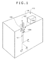
- FIG. 1 a schematic diagram of a borehole (or well bore) 102 in a formation 110 is shown.
- the formation 110 can contain a desirable fluid such as oil or gas.
- the borehole 102 is a vertical wellbore (e.g., parallel to the X 3 -axis) drilled in the formation 110.
- a vertical wellbore is shown in FIG. 1 as an example, it should be understood that the borehole 102 can optionally be a deviated or horizontal wellbore.
- the borehole 102 can be used to extract the desirable fluid.
- the borehole 102 can be a fluid-filled wellbore, e.g., filled with a drilling fluid 101.
- the borehole 102 can have an acoustic tool arranged therein.
- An acoustic tool (or logging tool, sonic tool, etc.) can include at least one acoustic source 106 and an array of acoustic receivers 108 (e.g., an acoustic array).
- the acoustic source 106 and the array of acoustic receivers 108 can be part of an acoustic logging tool of any type, including but not limited to, a wire-line logging tool, a LWD tool or a measurement while drilling ("MWD”) tool.
- Logging tools are well known in the art and are therefore not discussed in further detail below.
- the acoustic source 106 can be configured to excite monopole or dipole acoustic modes or other multipole acoustic modes. It should be understood that the acoustic source 106 is configured to transmit energy (e.g., acoustic waves) into the formation 110. The energy can be characterized by its frequency and wavelength. Optionally, the acoustic source 106 can transmit broadband energy at frequencies between 0.5 and 20kHz, for example. The transmitted energy can excite compressional, shear, Stoneley, flexural and/or multipole waves in the formation 110. Additionally, the array of acoustic receivers 108 is configured to detect the compressional, shear, Stoneley, flexural or multipole waves travelling in the drilling fluid 101, for example.
- energy e.g., acoustic waves
- the transmitted energy can excite compressional, shear, Stoneley, flexural and/or multipole waves in the formation 110.
- the array of acoustic receivers 108 is configured to detect
- the array of acoustic receivers 108 can optionally include a plurality of acoustic receivers. By arranging acoustic receivers in an array with different spacing from the acoustic source 106, it is possible to improve signal quality and extract various borehole signals over a broad frequency band.
- the borehole 102, as well as the acoustic source 106 and the array of acoustic receivers 108, are provided only as examples and are not intended to be limiting.
- the acoustic tool (e.g., the acoustic source 106 and the array of acoustic receivers 108) can be operably connected with one or more computing devices.
- computing device 120A can be located in the borehole, e.g., computing device 120A can be integrated with the acoustic tool.
- computing device 120B can optionally be located above, on and/or below the surface of the formation 110.
- the computing devices can be operably connected, and each computing device can be configured to perform some or all of the operations described below for generating slowness-frequency projection logs.
- the computing devices can optionally be configured to control the acoustic source 106 and/or the array of acoustic receivers 108, as well as receive, process and store sonic data (e.g., the acoustic data detected, collect, recorded, etc. by the acoustic receivers 108).
- each computing device typically includes at least one processing unit and system memory.
- system memory may be volatile (such as random access memory (RAM)), non-volatile (such as read-only memory (ROM), flash memory, etc.), or some combination of the two.
- the processing unit can be a standard programmable processor that performs arithmetic and logic operations necessary for operation of the computing devices.
- the processing unit can be configured to execute program code encoded in tangible, computer-readable media.
- Computer-readable media refers to any media that is capable of providing data that causes the computing devices (i.e., a machine) to operate in a particular fashion.
- Various computer-readable media may be utilized to provide instructions to the processing unit for execution.
- Example tangible, computer-readable recording media include, but are not limited to, an integrated circuit (e.g., field-programmable gate array or application-specific IC), a hard disk, an optical disk, a magneto-optical disk, a floppy disk, a magnetic tape, a holographic storage medium, a solid-state device, RAM, ROM, electrically erasable program read-only memory (EEPROM), flash memory or other memory technology, CD-ROM, digital versatile disks (DVD) or other optical storage, magnetic cassettes, magnetic tape, magnetic disk storage or other magnetic storage devices.
- an integrated circuit e.g., field-programmable gate array or application-specific IC
- a hard disk e.g., an optical disk, a magneto-optical disk, a floppy disk, a magnetic tape, a holographic storage medium, a solid-state device, RAM, ROM, electrically erasable program read-only memory (EEPROM), flash memory or other memory technology, CD-ROM, digital versatile disks (
- each computing device can have additional features/functionality.
- the computing devices may include additional storage such as removable storage and non-removable storage including, but not limited to, magnetic or optical disks or tapes.
- the computing devices may also contain network connection(s) that allow the device to communicate with other devices.
- the computing devices may also have input device(s) such as a keyboard, mouse, touch screen, etc.
- Output device(s) such as a display, speakers, printer, etc. may also be included.
- the additional devices may be connected to the bus in order to facilitate communication of data among the components of the computing devices. All these devices are well known in the art and need not be discussed at length here.
- dispersive modes or waves e.g., leaky-p, borehole flexural and/or borehole multipole modes
- downhole e.g., at the acoustic tool located in the borehole
- processing of such dispersive modes can be more complex than performing conventional monopole P&S and can result in more ambiguity and/or errors. It is therefore desirable to provide reliable, real-time, visual QC indicators when using information obtained by processing the dispersive modes.
- conventional techniques to provide QC indicators such as SFA are computationally expensive.
- FIG. 2A a graph illustrating example leaky-p waveforms measured by an acoustic array is shown.
- the leaky-p waveforms can be measured using the acoustic array shown in FIG. 1 , for example.
- Slowness-frequency dispersions can be extracted using a modified matrix-pencil algorithm, for example.
- a graph illustrating example slowness-frequency dispersions extracted from the waveforms of FIG. 2A using a modified matrix pencil algorithm is shown in FIG. 2B .
- a low frequency asymptote of the first order mode 202 indicates the formation compressional slowness.
- the second order mode 204 can be seen at approximately 6.5 kHz and above.
- a low frequency asymptote of the second order mode also indicates the formation compressional slowness.
- the computing power of a computing device located in the borehole is typically much less than the computing power of a computing device employed at the surface of the formation. This makes it practically difficult to provide conventional QC indicators, for example using conventional SFA techniques, using a computing device located in the borehole. Additionally, bandwidth between the acoustic tool located in the borehole and the surface of the formation is limited.
- the logical operations described herein with respect to the various figures may be implemented (1) as a sequence of computer implemented acts or program modules (i.e., software) running on a computing device, (2) as interconnected machine logic circuits or circuit modules (i.e., hardware) within the computing device and/or (3) a combination of software and hardware of the computing device.
- the logical operations discussed herein are not limited to any specific combination of hardware and software. The implementation is a matter of choice dependent on the performance and other requirements of the computing device. Accordingly, the logical operations described herein are referred to variously as operations, structural devices, acts, or modules. These operations, structural devices, acts and modules may be implemented in software, in firmware, in special purpose digital logic, and any combination thereof. It should also be appreciated that more or fewer operations may be performed than shown in the figures and described herein. These operations may also be performed in a different order than those described herein.
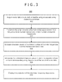
- FIG. 3 a flow diagram illustrating example operations 300 for generating slowness-frequency projection logs is shown.
- the example operations 300 can be implemented using the acoustic source 106, the array of acoustic receivers 108 and computing device 120A and/or computing device 120B shown in FIG. 1 , for example.
- sonic data is acquired at a plurality of depths using an acoustic array located in a borehole (e.g., acoustic receivers 108 of FIG. 1 ).
- acoustic waves can be generated using an acoustic source (e.g., acoustic source 106 of FIG. 1 ).
- the acoustic source can be one or more monopole, dipole and/or multipole acoustic sources. Additionally, the acquired sonic data can include dispersive modes such as leaky-p, borehole flexural and borehole multipole modes.
- the acquired sonic data is transformed from a time-space domain to a frequency-wave number domain at a limited number of discrete frequencies. For example, the limited number of discrete frequencies can be no more than two discrete frequencies. Alternatively, the limited number of discrete frequencies can optionally be greater than two, three or four discrete frequencies. Alternatively or additionally, the limited number of discrete frequencies can optionally be less than or equal to five discrete frequencies. It should be understood that the limited number of discrete frequencies provided above are only examples and that the limited number of discrete frequencies can optionally be greater than five discrete frequencies.
- the sonic data is transformed from the time-space domain to the frequency-wave number domain using a two-dimensional Fast Fourier Transform ("2D-FFT").
- the sonic data is transformed from the time-space domain to the frequency-wave number domain using a frequency domain Radon transform. It should be understood that the 2D-FFT and Radon transform are provided only as examples and that other known transforms can be used.
- slowness values at the limited number of discrete frequencies are estimated from the transformed sonic data.
- the slowness values at the limited number of discrete frequencies are optionally estimated from the transformed sonic data (e.g., sonic data in the frequency-wave number domain) based on a relationship between slowness, wave number and frequency.
- the relationship can be defined by Eqn. (1) below.
- s k f
- s slowness
- k wave number
- f frequency.
- the wave numbers can be converted to slowness values because wave numbers are related to slowness values by frequency.
- FIG. 4A A graph illustrating an example energy distribution over a frequency-slowness plane is shown in FIG. 4A . The graph illustrates the energy distribution with color variation over a frequency band between 0 and 10 kHz. As shown in FIG.
- FIG. 4A the energy distribution is calculated over the entire slowness range and the entire frequency range.
- FIG. 4A is provided only as an example. This disclosure contemplates that the energy distribution over the frequency-slowness plane can be calculated at a limited number of discrete frequencies according to steps 302-306 described above as opposed to over the entire frequency range.
- a graph illustrating an energy distribution as a function slowness at a select frequency (e.g., 5 kHz) is shown in FIG. 4B .
- the peak energy distribution at 5 kHz corresponds to a slowness of approximately 180 ⁇ s/ft.
- the peak energy distribution at one or more discrete frequencies e.g., 2.5, 3.5, 4.5, 5.5 and 6.5 kHz.
- the corresponding slowness at the peak energy distribution for each of the one or more discrete frequencies is plotted as markers 402, 404, 406, 408 and 410 in FIG. 4A .
- a line connecting these markers in FIG. 4A indicates the dispersive features of the mode, which is similar to the dispersion extracted using a modified matrix pencil algorithm shown in FIG. 2B .
- the estimated slowness values at the limited number of discrete frequencies can be transmitted, for example between a computing device located in the borehole (e.g., computing device 120A of FIG. 1 ) and a computing device located on the surface of the formation (e.g., computing device 120B of FIG. 1 ), before further processing.
- a computing device located in the borehole e.g., computing device 120A of FIG. 1
- a computing device located on the surface of the formation e.g., computing device 120B of FIG. 1
- a computing device with limited computing power e.g., a computing device incorporated in an acoustic tool located in a borehole
- a computing device incorporated in an acoustic tool is required to perform these processing steps within a limited time period, for example, the time period between firings of an acoustic source. Therefore, reducing the computing cost also facilitates the ability of the computing device to perform these processing steps within the limited time period.
- the communication link between the acoustic tool and the surface of the formation is typically bandwidth limited.
- this disclosure contemplates performing all of the steps for generating slowness-frequency projection logs with one or more computing devices without intermediate data transmission. For example, it is possible to perform all of the steps for generating slowness-frequency projection logs with one or more computing devices on the surface of the formation during LWD sonic logging applications or with one or more computing devices during wire-line sonic logging applications. In these cases, the computing cost and size of data transmission is reduced as compared to conventional techniques.
- the estimated slowness values at the limited number of discrete frequencies are interpolated to obtain a projection of one or more slowness-frequency dispersions of the acquired sonic data at 308.
- the projection of the slowness-frequency dispersions can be reproduced by interpolating between the estimated slowness values.
- step 308 can optionally be performed by a computing device located on the surface of the formation (e.g., computing device 120B of FIG. 1 ) after receiving the estimated slowness values.
- the projection of the slowness-frequency dispersions e.g., a slowness-frequency projection log
- the projection of the slowness-frequency dispersions is displayed, for example, on a display device.
- the projection of the slowness-frequency dispersions can include a plurality of color bands 502, 504, 506, 508 and 510 corresponding to each of the limited number of discrete frequencies.
- different colors are assigned to different discrete frequencies according to Table 1 below.
- Table 1 Frequency (kHz) Color Reference No. 2.5 Red 502 3.5 Yellow 504 4.5 Green 506 5.5 Cyan 508 6.5 Blue 510 It should be understood that the limited number of discrete frequencies and the assigned colors are provided as examples only and that more or fewer discrete frequencies and different assigned colors can be used.
- a width of each of the color bands can indicate a slowness dispersiveness of an acoustic mode.
- color variation of the color bands can indicate variability of the slowness-frequency dispersions depending on frequency.
- the measured waves are less dispersive above 1124 m (e.g., depths less than 1124 m) because width of the slowness-frequency projection is relatively narrow at these depths.
- the measured waves become more dispersive in the deeper zone (e.g., depths greater than 1124 m).
- compressional or shear slowness logs can be estimated from the acquired sonic data according to any known technique.
- the projection of the slowness-frequency dispersions can optionally be displayed or overlaid on the compressional or shear slowness logs.
- the projection of the slowness-frequency dispersions provides a QC indicator of compressional slowness.
- the projection of the slowness-frequency dispersions provides a QC indicator of shear slowness.
- the estimated compressional slowness log is shown by line 520. It should be understood that the slowness-frequency projection log provides a QC indicator for the estimated compressional slowness log.
- the estimated compressional slowness log matches the zero-frequency limit of the projection
- the estimated compressional slowness log crosses the projection
- the estimated compressional slowness is inaccurate.
- the estimated compressional slowness 520 is located slightly to the left of the color bands 502-510. This means that the estimated compressional slowness is accurate.
- the compressional slowness obtained from the sonic data properly picks up the low frequency asymptote of the dispersive mode.
Landscapes
- Physics & Mathematics (AREA)
- Life Sciences & Earth Sciences (AREA)
- Engineering & Computer Science (AREA)
- Remote Sensing (AREA)
- Geology (AREA)
- Environmental & Geological Engineering (AREA)
- Acoustics & Sound (AREA)
- General Life Sciences & Earth Sciences (AREA)
- General Physics & Mathematics (AREA)
- Geophysics (AREA)
- Geophysics And Detection Of Objects (AREA)
- Measurement Of Velocity Or Position Using Acoustic Or Ultrasonic Waves (AREA)
- Investigating Or Analyzing Materials By The Use Of Ultrasonic Waves (AREA)
Applications Claiming Priority (2)
| Application Number | Priority Date | Filing Date | Title |
|---|---|---|---|
| US201361862071P | 2013-08-04 | 2013-08-04 | |
| US14/341,847 US9746568B2 (en) | 2013-08-04 | 2014-07-28 | Methods, systems and devices for generating slowness-frequency projection logs |
Publications (2)
| Publication Number | Publication Date |
|---|---|
| EP2835665A2 true EP2835665A2 (de) | 2015-02-11 |
| EP2835665A3 EP2835665A3 (de) | 2015-12-09 |
Family
ID=51257426
Family Applications (1)
| Application Number | Title | Priority Date | Filing Date |
|---|---|---|---|
| EP14179535.1A Withdrawn EP2835665A3 (de) | 2013-08-04 | 2014-08-01 | Verfahren, Systeme und Vorrichtungen zur Erzeugung von Langsamkeitsfrequenz-Projektionsprotokollen |
Country Status (5)
| Country | Link |
|---|---|
| US (1) | US9746568B2 (de) |
| EP (1) | EP2835665A3 (de) |
| AU (1) | AU2014208222A1 (de) |
| BR (1) | BR102014019251A2 (de) |
| MX (1) | MX351087B (de) |
Cited By (2)
| Publication number | Priority date | Publication date | Assignee | Title |
|---|---|---|---|---|
| FR3085054A1 (fr) * | 2017-12-12 | 2020-02-21 | Services Petroliers Schlumberger | Procédés et appareil pour caractériser des dispersions acoustiques dans un puits de forage |
| CN115061205A (zh) * | 2021-03-08 | 2022-09-16 | 中国石油天然气股份有限公司 | 慢度的去噪方法、装置、电子设备以及存储介质 |
Families Citing this family (8)
| Publication number | Priority date | Publication date | Assignee | Title |
|---|---|---|---|---|
| FR3049355B1 (fr) | 2016-03-25 | 2020-06-12 | Services Petroliers Schlmumberger | Procede et dispositif d'estimation de la lenteur acoustique dans une formation souterraine |
| EP3861378B1 (de) * | 2018-10-01 | 2024-12-04 | Services Pétroliers Schlumberger | Verfahren und vorrichtung zur bestimmung von akustischer langsamkeit |
| WO2021257097A1 (en) | 2020-06-19 | 2021-12-23 | Halliburton Energy Services, Inc. | Acoustic dispersion curve identification based on reciprocal condition number |
| CN115166817B (zh) * | 2022-06-30 | 2023-02-17 | 哈尔滨工程大学 | 一种基于冰层模态群慢度差特征的冰声定位方法 |
| CN115407405B (zh) * | 2022-08-25 | 2025-08-22 | 中国电波传播研究所(中国电子科技集团公司第二十二研究所) | 一种实验室内阵列声波慢度计算方法 |
| CN115616662A (zh) * | 2022-09-13 | 2023-01-17 | 西南石油大学 | 一种基于ista的高分辨率radon变换的面波频散能量谱成像方法 |
| CN120143265B (zh) * | 2023-12-11 | 2025-11-18 | 中国石油天然气集团有限公司 | 地层压裂检测方法、装置、处理器及存储介质 |
| CN120254968B (zh) * | 2025-06-05 | 2025-08-12 | 中海油田服务股份有限公司 | 基于频域分析的井孔声波速度获取方法及装置 |
Citations (1)
| Publication number | Priority date | Publication date | Assignee | Title |
|---|---|---|---|---|
| US7643374B2 (en) | 2004-02-27 | 2010-01-05 | Schlumberger Technology Corporation | Slowness-frequency projection display and animation |
Family Cites Families (1)
| Publication number | Priority date | Publication date | Assignee | Title |
|---|---|---|---|---|
| US8848484B2 (en) | 2010-12-08 | 2014-09-30 | Schlumberger Technology Corporation | Filtering acoustic waveforms in downhole environments |
-
2014
- 2014-07-28 US US14/341,847 patent/US9746568B2/en active Active
- 2014-07-30 AU AU2014208222A patent/AU2014208222A1/en not_active Abandoned
- 2014-08-01 EP EP14179535.1A patent/EP2835665A3/de not_active Withdrawn
- 2014-08-04 BR BR102014019251A patent/BR102014019251A2/pt not_active IP Right Cessation
- 2014-08-04 MX MX2014009407A patent/MX351087B/es active IP Right Grant
Patent Citations (1)
| Publication number | Priority date | Publication date | Assignee | Title |
|---|---|---|---|---|
| US7643374B2 (en) | 2004-02-27 | 2010-01-05 | Schlumberger Technology Corporation | Slowness-frequency projection display and animation |
Non-Patent Citations (1)
| Title |
|---|
| EKSTROM, M.P.: "Dispersion Estimation From Borehole Acoustic Arrays Using a Modified Matrix Pencil Algorithm", 29TH ASILOMAR CONFERENCE ON SIGNALS, SYSTEMS, AND COMPUTERS, 1995 |
Cited By (2)
| Publication number | Priority date | Publication date | Assignee | Title |
|---|---|---|---|---|
| FR3085054A1 (fr) * | 2017-12-12 | 2020-02-21 | Services Petroliers Schlumberger | Procédés et appareil pour caractériser des dispersions acoustiques dans un puits de forage |
| CN115061205A (zh) * | 2021-03-08 | 2022-09-16 | 中国石油天然气股份有限公司 | 慢度的去噪方法、装置、电子设备以及存储介质 |
Also Published As
| Publication number | Publication date |
|---|---|
| MX2014009407A (es) | 2015-05-27 |
| US9746568B2 (en) | 2017-08-29 |
| US20150036460A1 (en) | 2015-02-05 |
| MX351087B (es) | 2017-09-29 |
| AU2014208222A1 (en) | 2015-02-19 |
| EP2835665A3 (de) | 2015-12-09 |
| BR102014019251A2 (pt) | 2016-03-15 |
Similar Documents
| Publication | Publication Date | Title |
|---|---|---|
| US9746568B2 (en) | Methods, systems and devices for generating slowness-frequency projection logs | |
| US11385374B2 (en) | Borehole dispersive wave processing with automatic dispersion matching for compressional and shear slowness | |
| CN103726836B (zh) | 基于声波测井资料提取模式波慢度的方法 | |
| US11230922B2 (en) | Fracture interpretation with resistivity and sonic logs in biaxial anisotropic formations | |
| US9631483B2 (en) | Joint time-frequency processing for borehole acoustic arrays | |
| US10564304B2 (en) | Processing methodology for full-waveform sonic wavefield separation | |
| US10197692B2 (en) | Validation of depth-depth curves using time-seismic depth interval velocity | |
| US20030206487A1 (en) | Acoustic logging apparatus and method | |
| AU2012396820A1 (en) | Method and system for direct slowness determination of dispersive waves in a wellbore environment | |
| US8451688B2 (en) | Methods and apparatus to combine monopole and multipole acoustic logging measurements to determine shear slowness | |
| US11237288B2 (en) | Verifying measurements of elastic anisotropy parameters in an anisotropic wellbore environment | |
| US12038546B2 (en) | Methods to estimate formation slowness from multi-borehole modes and of a multi-mode dispersion wave and multi-mode dispersion estimation systems | |
| US20170183962A1 (en) | Identifying Formation Layer Boundaries on Well Log Measurements | |
| US10955581B2 (en) | Using an adjusted drive pulse in formation evaluation | |
| CN112649876A (zh) | 建立地震偏移速度模型的方法和装置 | |
| WO2016209265A1 (en) | Identifying formation layer boundaries on well log measurements | |
| Sadala Valente et al. | Time-to-depth conversion and velocity estimation by image-wavefront propagation | |
| NL2034841B1 (en) | Method and device for converting seismic datasets | |
| NO20190412A1 (en) | Avoiding Geological Bodies that are Hazards to Drilling Operations | |
| Collins et al. | Improved Stoneley Wave Inversion Method for Fracture Evaluation | |
| Valero et al. | High resolution compressional slowness log estimation using first motion detection |
Legal Events
| Date | Code | Title | Description |
|---|---|---|---|
| PUAI | Public reference made under article 153(3) epc to a published international application that has entered the european phase |
Free format text: ORIGINAL CODE: 0009012 |
|
| 17P | Request for examination filed |
Effective date: 20140801 |
|
| AK | Designated contracting states |
Kind code of ref document: A2 Designated state(s): AL AT BE BG CH CY CZ DE DK EE ES FI FR GB GR HR HU IE IS IT LI LT LU LV MC MK MT NL NO PL PT RO RS SE SI SK SM TR |
|
| AX | Request for extension of the european patent |
Extension state: BA ME |
|
| PUAL | Search report despatched |
Free format text: ORIGINAL CODE: 0009013 |
|
| AK | Designated contracting states |
Kind code of ref document: A3 Designated state(s): AL AT BE BG CH CY CZ DE DK EE ES FI FR GB GR HR HU IE IS IT LI LT LU LV MC MK MT NL NO PL PT RO RS SE SI SK SM TR |
|
| AX | Request for extension of the european patent |
Extension state: BA ME |
|
| RIC1 | Information provided on ipc code assigned before grant |
Ipc: G01V 1/48 20060101AFI20151030BHEP |
|
| STAA | Information on the status of an ep patent application or granted ep patent |
Free format text: STATUS: THE APPLICATION IS DEEMED TO BE WITHDRAWN |
|
| 18D | Application deemed to be withdrawn |
Effective date: 20160610 |