EP2767862B1 - Prescription-dependent and individualization-dependent adaptation of the object distance function to changed object distances for near and/or far vision - Google Patents
Prescription-dependent and individualization-dependent adaptation of the object distance function to changed object distances for near and/or far vision Download PDFInfo
- Publication number
- EP2767862B1 EP2767862B1 EP14001194.1A EP14001194A EP2767862B1 EP 2767862 B1 EP2767862 B1 EP 2767862B1 EP 14001194 A EP14001194 A EP 14001194A EP 2767862 B1 EP2767862 B1 EP 2767862B1
- Authority
- EP
- European Patent Office
- Prior art keywords
- function
- object distance
- spectacle lens
- korr
- target
- Prior art date
- Legal status (The legal status is an assumption and is not a legal conclusion. Google has not performed a legal analysis and makes no representation as to the accuracy of the status listed.)
- Active
Links
- 230000006978 adaptation Effects 0.000 title description 10
- 230000004438 eyesight Effects 0.000 title description 9
- 230000001419 dependent effect Effects 0.000 title description 4
- 230000000750 progressive effect Effects 0.000 claims description 101
- 238000000034 method Methods 0.000 claims description 45
- 238000012937 correction Methods 0.000 claims description 38
- 238000004590 computer program Methods 0.000 claims description 10
- 238000004519 manufacturing process Methods 0.000 claims description 10
- 238000012886 linear function Methods 0.000 claims description 7
- 238000003860 storage Methods 0.000 claims description 6
- 230000004048 modification Effects 0.000 claims description 4
- 238000012986 modification Methods 0.000 claims description 4
- 238000003754 machining Methods 0.000 claims 2
- 230000006870 function Effects 0.000 description 265
- 201000009310 astigmatism Diseases 0.000 description 201
- 238000009826 distribution Methods 0.000 description 101
- 238000007792 addition Methods 0.000 description 53
- 238000013461 design Methods 0.000 description 48
- 230000002123 temporal effect Effects 0.000 description 45
- 238000005457 optimization Methods 0.000 description 33
- 208000014733 refractive error Diseases 0.000 description 15
- 238000004364 calculation method Methods 0.000 description 10
- 230000008859 change Effects 0.000 description 10
- 238000011156 evaluation Methods 0.000 description 9
- 230000009466 transformation Effects 0.000 description 9
- 230000004075 alteration Effects 0.000 description 6
- 239000011521 glass Substances 0.000 description 6
- 230000003287 optical effect Effects 0.000 description 6
- 230000000694 effects Effects 0.000 description 5
- 230000001131 transforming effect Effects 0.000 description 5
- 238000001514 detection method Methods 0.000 description 4
- 238000012545 processing Methods 0.000 description 4
- 230000001179 pupillary effect Effects 0.000 description 4
- 238000003384 imaging method Methods 0.000 description 3
- 230000002452 interceptive effect Effects 0.000 description 3
- 230000007704 transition Effects 0.000 description 3
- 230000008901 benefit Effects 0.000 description 2
- 230000000052 comparative effect Effects 0.000 description 2
- 230000002093 peripheral effect Effects 0.000 description 2
- 230000008569 process Effects 0.000 description 2
- 210000001747 pupil Anatomy 0.000 description 2
- 238000000844 transformation Methods 0.000 description 2
- 230000000007 visual effect Effects 0.000 description 2
- 101100042630 Caenorhabditis elegans sin-3 gene Proteins 0.000 description 1
- 230000004308 accommodation Effects 0.000 description 1
- 230000009471 action Effects 0.000 description 1
- 238000005266 casting Methods 0.000 description 1
- 238000004891 communication Methods 0.000 description 1
- 238000010276 construction Methods 0.000 description 1
- 238000007796 conventional method Methods 0.000 description 1
- 238000009795 derivation Methods 0.000 description 1
- 230000009977 dual effect Effects 0.000 description 1
- 230000004418 eye rotation Effects 0.000 description 1
- 230000001771 impaired effect Effects 0.000 description 1
- 208000001491 myopia Diseases 0.000 description 1
- 230000002265 prevention Effects 0.000 description 1
- 230000009467 reduction Effects 0.000 description 1
- 230000004044 response Effects 0.000 description 1
- 230000005477 standard model Effects 0.000 description 1
- 230000029305 taxis Effects 0.000 description 1
Images


Classifications
-
- G—PHYSICS
- G02—OPTICS
- G02C—SPECTACLES; SUNGLASSES OR GOGGLES INSOFAR AS THEY HAVE THE SAME FEATURES AS SPECTACLES; CONTACT LENSES
- G02C7/00—Optical parts
- G02C7/02—Lenses; Lens systems ; Methods of designing lenses
- G02C7/024—Methods of designing ophthalmic lenses
- G02C7/028—Special mathematical design techniques
-
- G—PHYSICS
- G02—OPTICS
- G02C—SPECTACLES; SUNGLASSES OR GOGGLES INSOFAR AS THEY HAVE THE SAME FEATURES AS SPECTACLES; CONTACT LENSES
- G02C7/00—Optical parts
- G02C7/02—Lenses; Lens systems ; Methods of designing lenses
- G02C7/06—Lenses; Lens systems ; Methods of designing lenses bifocal; multifocal ; progressive
- G02C7/061—Spectacle lenses with progressively varying focal power
- G02C7/063—Shape of the progressive surface
- G02C7/065—Properties on the principal line
Definitions
- aspects of the present invention relate to computer-implemented methods for optimizing and manufacturing a progressive spectacle lens, to corresponding devices for optimizing and producing a progressive spectacle lens, to corresponding computer program products and to storage media.
- optimization of a progressive spectacle lens is usually accomplished by minimizing a target function in which target values for at least one optical variable, e.g. Astigmatism and / or refractive power, or target values for at least one aberration, e.g. astigmatic error and / or refractive error, the progressive spectacle lens.
- target values for at least one optical variable e.g. Astigmatism and / or refractive power, or target values for at least one aberration, e.g. astigmatic error and / or refractive error
- the individual prescription values e.g. Astigmatism and / or refractive power
- target values for at least one aberration e.g. astigmatic error and / or refractive error
- the progressive spectacle lens the individual prescription values (sph, cyl, axis, add, prism, base), parameters of the individual position or arrangement of the spectacle lens in front of the wearer's eye (eg corneal vertex distance (HSA), lens angle (FSW), pret
- DE 10 2008 015 189 DE 10 2009 005 206 or DE 10 2009 005 214 It has also been proposed to determine the desired astigmatism distribution on the basis of which the progressive spectacle lens is optimized by means of a transformation of an existing or predetermined design (start design, basic design). So will in DE 10 2008 015 189 proposed to calculate target astigmatism distributions for different additions by means of a transformation of a given base or start target astigmatism distribution which has been determined for a given base addition.
- DE 10 2009 005 206 or DE 10 2009 005 214 It is proposed to generate target astigmatism distributions with different widths of the far and / or near range from a predefined target astigmatism distribution by means of a manipulation of a predefined basic target isoastigmatism line.
- DE 10 2008 015 189 DE 10 2009 005 206 or DE 10 2009 005 214 described methods make it possible to simplify the process for optimizing a progressive spectacle lens and make it more efficient and flexible.
- the WO 2008/089996 discloses a computer-implemented method for calculating a prescription lens design for an individual progressive prescription lens having a variably adjustable, individual vertical position of the distance and / or the near reference point. It is an object of the invention to provide improved methods for optimizing and manufacturing progressive spectacle lenses.
- This object is achieved by a computer-implemented method for optimizing a progressive spectacle lens having the features of claim 1, a computer program product having the features of claim 7, a storage medium having stored thereon computer program having the features of claim 8, an apparatus for optimizing a progressive spectacle lens with the features of claim 9, a method for producing a progressive spectacle lens having the features of claim 10 and an apparatus for producing a progressive spectacle lens having the features of claim 11.
- the optimization of progressive spectacle lenses is generally carried out by minimizing a target function in which target values for at least one optical variable (eg astigmatism and / or refractive power) or target values for at least one aberration (eg astigmatic error or astigmatic deviation and / or refractive error) of the progressive spectacle lens.
- the target values or target values of the at least one optical property or of the at least one aberration that enter the target function characterize the design of a spectacle lens.
- the eyeglass lens design may include a suitable object distance model.
- the object distance model may include an object distance function defined as the reciprocal object distance along the main line of sight.
- a standardized object distance model is e.g. in DIN 58 208 Part 2 (see Figure 6). However, the object distance model may differ from this standard object distance model.
- a main line of vision is the sequence of puncture points of the main rays through the respective lens surface when looking at a line which lies in the vertical plane, which halves the distance between the two eye rotation points (so-called cyclopenoid plane).
- the spectacle lens surface may be the object or the eye-side surface. The position of the line in the cyclops-eye plane is determined by the selected object distance model.
- a main line is understood to mean a line which runs essentially straight or helical, along which the desired increase in the refractive power of the spectacle lens from the distance to the near portion is achieved.
- the main line extends substantially centrally to the spectacle lens from top to bottom, that is, along a substantially vertical direction.
- the main line thus represents a construction line in the coordinate system of the object-side or eye-side surface to be optimized for describing the desired values.
- the course of the main line of the spectacle lens is chosen such that it follows at least approximately the main line of vision.
- a method of fitting the main line to the main line of vision is described, for example, in US Pat EP 1 277 079 A2 described.
- the object distance function (ie the reciprocal object distance at the main line of sight) plays an essential role in the design specification and optimization of progressive spectacle lenses.
- the basic characteristic of a progressive spectacle lens in the vicinity of the main line of sight is predominantly determined by the course of the object distance function A 1 ( y ) along the main line of vision.
- the object distance data including an object distance in at least one predetermined point on the main view line; Modifying or transforming the start-to-space distance function in response to the acquired object range data; and Optimizing the progressive spectacle lens, wherein the modified / transformed object distance function is taken into account in the optimization of the spectacle lens, includes.
- Modifying / transforming the starting distance function A 1 G ( y ) comprises superimposing the start distance function A 1 G ( y ) with a correction function A 1 Korr ( y ):
- a 1 y A 1 G y + A 1 corr y ,
- the object distance function represents the reciprocal object distance (the reciprocal object distance) along the main line of sight as a function of the vertical coordinate y .
- the object distance function is defined as the reciprocal object distance (the reciprocal object distance) along the main line of sight.
- the correction function has at least one variable parameter, which is determined in dependence on the acquired object distance data such that the value of the modified start distance function in at least one predetermined point is equal to the reciprocal value of the detected solar object distance for that point.
- the coordinate system can be any coordinate system, in particular one of the previously described coordinate systems ⁇ x , y ⁇ or ⁇ u, y ⁇ , where u represents the distance from the main sight line or main line.
- the object removal data comprises at least one Solobject distance A 1 Distance in a given distance reference point (design point distance) DF on the main sight line and a sol object distance A 1 Proximity in a given near reference point (design point proximity) DN on the main sight line.
- the at least one variable parameter of the correction function is determined or determined in such a way that the respective value of the modified start-distance function at the far and / or near reference point is equal to the corresponding reciprocal value of the detected target distance for the far and / or near reference point.
- the parameters a G , b G can therefore be determined automatically in the distance and near reference points DF and DN using the standard specifications for the reciprocal object distances A 1 GFerne and A 1 GN .
- a standard object distance model is specified, for example, in DIN 58 208 Part 2.
- the start object distance function is superimposed with a correction function in order to take this change into account.
- start object distance function can be overlaid with other functions, for example, to achieve a targeted modification of the design characteristics.
- At least one of the parameters of the correction function is variable and is included in Dependent on the detected object distance data, in particular determined or fixed by the changed setpoint values for the object distances in the far and / or near reference point.
- variable parameters / coefficients b corr and a corr of the correction function are determined or established as a function of the acquired object distance data.
- both the start-distance function and the correction function are dual asymptote functions.
- the coefficients / parameters of the starting distance function (basic function) and the coefficients / parameters of the correction function can be determined beforehand and preferably stored separately in a memory as data files. This allows easy subsequent reproduction and modification of the values of the startup design.
- the start-object distance function which may be a double asymptotic function in particular, may be in addition to a superposition with a correction function A 1 Korr ( y ) - with a function in the form of a Gaussian bell curve
- start distance function is a double asymptotic function
- start distance function is a double asymptotic function
- the curve characteristic of the start-object distance function can be modified in a targeted manner.
- the Gaussian function causes the object distance function to be flatter above the gauss maximum.
- the refractive index change is reduced in this range, the isoastigmatism lines move farther outward and the substantially defect-free glass region, e.g. the glass area with an astigmatic error smaller than 0.5 D becomes wider.
- areas e.g., the intermediate area
- the percentage weight g G and the other coefficients of the Gaussian function can be specified for the respective basic design or eg based on the in WO 2010/084019 be determined method based on a design polygon.
- the parameter y 0 is preferably in the range -10 ⁇ y 0 ⁇ 5, more preferably in the range -5 ⁇ y 0 ⁇ 0.
- the parameter ⁇ is preferably in the range 0 ⁇ ⁇ ⁇ 15, further preferably in the range 5 ⁇ ⁇ 10.
- the superimposition of the start-distance function with a Gaussian bell curve can, according to a further aspect, take place independently of an overlay with a correction function.
- the straight line coefficients c and m are calculated from the deviations of the values of the start distance function A 1G ( y ) from the detected set points of the reciprocal distance in the far and near reference points.
- the start-distance function there is a linear adaptation of the start-distance function to the changed object distances in the far and / or in the near reference point.
- This adjusted object distance function which is a linear function of the start-to-object distance function, does not substantially change the course of the reciprocal object distance along the main line of sight.
- the first derivative of the starting distance function is only changed by a factor (1 + m ).
- the basic characteristic of a progressive spectacle lens in the vicinity of the main sight line becomes predominantly due to the course of the object distance function A 1 ( y ) determined along the main line of sight (Minkwitz's theorem).
- the linear adaptation of the start-object distance function makes it possible to obtain the design characteristic very well even with an adaptation of the object distances to changed specifications in one or two points with negligible computation effort.
- the method described above can be applied independently of the course of the reciprocal object distance along the main sight line. It is also possible to substantially maintain the characteristic of the object distance function along the main line of sight while at the same time design-varying the object distances in the design points / reference points or adapting them to the needs or wishes of the spectacle wearer.
- the starting object distance function (basic function) A 1 G ( y ) may be any analytical function or also an interpolation function (spline function). There are no coefficients of the basic function to be known or modified. If A 1 G ( y ) specified pointwise or, as in the patent application DE 10 2009 005 847.8 described, is modified before the optimization, this method is particularly well suited for matching the object distance function to the individual Solumblejektentfernonne in the design points or reference points.
- the optimization of progressive spectacle lenses is generally carried out by an iterative minimization of a target function in which target values for at least one optical variable (eg astigmatism and / or refractive power) or target values for at least one aberration (eg astigmatic error and / or refractive error) of the progressive spectacle lens.
- the refractive error represents the difference of the refractive power of the spectacle lens from the refractive power, which is determined by refraction determination.
- the astigmatic error represents the difference of the astigmatism of the spectacle lens from The astigmatism, which is determined by means of refraction determination, is.
- These are preferably values in the position of use of the spectacle lens, ie, taking into account the system spectacle lens-eye.
- Degree of freedom in the optimization of the objective function is usually the arrow height of the front or the rear surface of the spectacle lens or both the front and the rear surface, for example, in a double-progressive spectacle lens.
- the actual and desired values of the at least one optical property entering the target function can be setpoints (area values or values in the use position) of the spectacle lens as well as setpoint values for at least one aberration.
- target astigmatism is therefore understood to mean both the astigmatism of the spectacle lens (as surface refractive power or in the position of use) and the astigmatic error.
- target astigmatism distribution in the context of this application means both the spatial distribution of the nominal values of the astigmatism of the spectacle lens and the spatial distribution of the nominal values of the astigmatic error.
- the nominal values of the at least one optical property of the spectacle lens and in particular the nominal values of the astigmatism or the astigmatic error characterize the "design" of a spectacle lens.
- the eyeglass lens design may include a suitable object distance model.
- the object distance model may include an object distance function defined as the reciprocal object distance along the main line of sight.
- a standardized object distance model is e.g. in DIN 58 208 Part 2 (see Figure 6).
- the object distance model may differ from this standard object distance model.
- the target astigmatism distribution on the basis of which the progressive spectacle lens is optimized, can be obtained by means of a transformation of an existing or predetermined design (start design, basic design).
- start design basic design
- DE 10 2008 015 189 proposed to obtain target astigmatism distributions for different additions by means of a transformation of a given base or starting roll astigmatism distribution established for a given base addition.
- DE 10 2009 005 206 or DE 10 2009 005 214 It is proposed, by means of a manipulation of a predetermined base target isoastigmatism line, to distribute target astigmatism with different Generate widths of the far and / or near range from a predetermined Sollastigmatismusverotti.
- the effect dependence of the target astigmatism can be covered by different basic designs.
- the startup design (base design) generally exhibits an approximately symmetrical distribution of the target astigmatism with respect to the main line of sight due to the binocular imaging properties. In the case of an addition and / or action and / or progression-length-dependent transformation of the start design, the approximately symmetrical distribution of the target astigmatism is essentially maintained.
- the temporal target astigmatism in the periphery of the spectacle lens is multiplied by a factor k in order to take this circumstance into account.
- the factor k preferably assumes the value 1 if no manipulation of the target astigmatism values is to take place and a value smaller than 1 if the target astigmatism values are to be manipulated.
- the factor k is a function of at least one prescription value (such as sphere, cylinder, cylinder axis, prism, prism base and / or addition) and / or at least one parameter of the spectacle lens or its arrangement in front of the wearer's eyes (ie its position of use).
- the parameters of the spectacle lens and / or its arrangement in front of the spectacle wearer are for example the mounting disc angle, the tilt angle, the corneal vertex distance (HSA), the pretilt or the pantoscopic angle, the pupil distance, the eye pivot distance and / or other parameters , These may be average values (as defined, for example, in DIN 58 208 Part 2) or values determined individually for a specific spectacle wearer.
- the start target astigmatism distribution Ast start via the spectacle lens may be the desired astigmatism distribution of a given progressive starting surface.
- a target astigmatism model can be specified, by means of which the starting target astigmatism distribution can be calculated.
- the Sollastigmatismusmodell can, for example, in the DE 10 2008 015 189 .
- DE 10 2009 005 206 or DE 10 2009 005 214 be described Sollastigmatismusmodell.
- the course of a main line as well as the course of at least one base target isoastigmatism line can be predefined parametrically or numerically.
- All desired astigmatism values between the main line and the base target isoastigmatism line as well as all desired astigmatism values between the base target isoastigmatism line and the periphery of the spectacle lens can subsequently be determined by suitable interpolations (eg linear, quadratic, cubic interpolation) of the predetermined target astigmatism values on the main line and the base target isoastigmatism line and possibly other predetermined values are determined, as in DE 10 2009 005 206 or DE 10 2009 005 214 described.
- suitable interpolations eg linear, quadratic, cubic interpolation
- a new, transformed target astigmatism distribution branch to New is a new, transformed target astigmatism distribution branch to New determined.
- the nominal nasal astigmatism values or the nominal nasal astigmatism distribution are preferably not changed.
- the new, transformed astigmatism distribution branch is to New by means of interpolation of the target astigmatism values between a predetermined temporal base isoastigmatism line (the 0.5 D base isoastigmatism line in the rule) and the periphery of the lens obtained, wherein the modified value of the maximum, temporal astigmatism max_Ast target temporal _ is newly considered.
- the pamphlets DE 10 2009 005 206 or DE 10 2009 005 214 describe respectively methods (parallel curve model method or truncated cone model method) for calculating a target astigmatism distribution from a given base target isoastigmatism line and the maximum temporal astigmatism.
- the predetermined 0.5 d base target isoastigmatism line can be determined from the starting target astigmatism distribution.
- the temporal target astigmatism values between the main line and the temporal base target isoastigmatism line are preferably not changed in this case.
- the new, transformed target astigmatism distribution generally has lower gradients of the target astigmatism in the periphery.
- transforming the start-target astigmatism distribution comprises branch target begin based on the modified temporal maximum astigmatism max_Ast target _temporal new hence an interpolation of the target astigmatism values between a predetermined base isoastigmatism line and the periphery of the spectacle lens, taking into account the modified maximum temporal astigmatism max_Ast , _temporal new .
- the spectacle lens optimization specifications including the target target astigmatism distribution and the transformed target astigmatism distribution Ast Soll New , can be specified in a suitable coordinate system.
- An exemplary coordinate system is a coordinate system in the object-side or eye-side surface of the spectacle lens to be optimized, wherein the origin of the coordinate system coincides, for example, with the geometric center of the tubular spectacle lens or with the centering or fitting point of the spectacle lens.
- the vertical (“ y ") and horizontal ("x") axes lie in the tangential plane to the respective eye-side or object-side surface of the spectacle lens in the geometric center and the fitting point, respectively.
- the vertical direction preferably refers to the vertical direction in the position of use of the spectacle lens, the spectacle lens being arranged, for example, in an average position of use (as defined, for example, in DIN 58 208 Part 2) or in an individual position of use.
- the spectacle lens is arranged in an individual use position.
- branch setpoint start branch setpoint applies begin ( x , y )
- branch setpoint New Branch target New ( x, y ).
- the setpoint values or the optimization setpoint values are predefined with respect to the main line, then it is only sufficient to adjust the position of use of the spectacle lens to be taken into account, and especially if the pupil distance, the corneal vertex distance, the pretilt, the object distance model, etc., change the main line to the modified main sight line.
- the setpoints or the optimization setpoints are then adjusted automatically.
- the asymptotic pre-factor v can be set such that the manipulation factor k is only applied to negative glasses.
- the pre-factor v can be a double asymptotic function of the remote regulation, and / or the base curve of the spectacle lens and / or the curvature of the rear surface of the spectacle lens.
- the function g Regulation is a function of the prescription astigmatism and / or the prescribed cylinder axis and / or the prescribed addition.
- the prescription astigmatism, the prescribed cylinder axis and the prescribed addition are the predetermined values which are determined, for example, by refraction determination by an optician or an ophthalmologist.
- the method preferably comprises a step of detecting the prescription values, in particular the prescription astigmatism, and / or the prescribed cylinder axis, and / or the prescribed addition.
- the parameter a is preferably in the range of 0.05 to 1.0, more preferably in the range 0.3 to 0.6, and particularly preferably takes the value 0.4.
- the parameter b is preferably in the range 2 to 6, and more preferably in the range 4 to 6. Particularly preferably, b assumes the value of the maximum prescription astigmatism.
- the straight line parameter c is preferably in the range between 0 and -1 and more preferably in the range between -0.75 and -0.3. Particularly preferably c assumes a value of -0.3636.
- the parameter d is preferably in the range from 2.0 to 0, more preferably in the range between 2 and 1. Particularly preferably, d assumes the value 1.2727.
- the function g regulation is preferably obtained by a multiplication of at least two of the factors f ( cylinder axis ) , f (prescription astigmatism ) and f ( addition ) , preferably by a multiplication of all three factors.
- g is a given constant. Since the influence of the tilt angle is not very large, g is preferably in the range of 50 to 500, more preferably in the range of 100 to 300, and particularly preferably in the value of about 200.
- the tilt angle is the angle which is the horizontal tangent of the object-side surface of the lens at a predetermined reference point and a horizontal reference line.
- the predetermined reference point is the intersection of the eye-side horizontal main beam in the zero viewing direction of the user with the object-side surface of the spectacle lens.
- the horizontal reference straight line lies in a plane which is perpendicular to the horizontal main ray in the zero viewing direction of the spectacle wearer.
- the tilt angle is one of the parameters of the arrangement of the lens in front of the eyes of the wearer.
- the individual factors or functions f are respectively calculated according to the equations (25) to (29).
- An advantage of a factor k calculated according to the formulas (30) or (31) is that the factor k automatically assumes a value of 1 if no transformation of the starting target astigmatism distribution is to take place.
- the factor k is preferably used only for prescription cylinder axis positions from 0 to 90 ° according to Tabo when specifying in positive-cylinder notation for right-hand lenses, for left-hand lenses in axial positions from 90 to 180 °. In Zylinderachslagen in these areas, the disadvantages described above occur increasingly. If the cylinder axis positions are in the other quadrants, then the optimization of the spectacle lens according to the conventional method (eg with the in DE 10 2008 015 189 disclosed method) taking into account a symmetrical Sollastigmatismusvorgabe.
- the desired astigmatism values can optionally be further scaled or transformed.
- the progression length may depend on the addition analogous to f ( addition ) , as in DE 10 2008 015 189 described.
- the target astigmatism values may be scaled as a function of the addition, such as in DE 10 2008 015 189 described.
- the order of the different scaling / transformations of the starting target astigmatism distribution may also vary.
- the distribution of the target refractive power or the target refractive error can be determined similarly to the target astigmatism distribution from a starting target refractive power distribution or a starting target refractive error distribution and varied by multiplication by a factor.
- the distribution of the setpoint value or the desired refraction error can likewise be determined on the basis of the previously determined, transformed desired astigmatism distribution.
- the optimization of the spectacle lens preferably takes place in the position of use of the spectacle lens.
- parameters of the individual position or arrangement of the spectacle lens in front of the eye wearer's eye eg corneal vertex distance (HSA), lens angle (FSW) , Preadjustment or pantoscopic angle
- / or physiological parameters of the wearer of the spectacle eg pupillary distance
- average parameters of the position or position of the spectacle lens in front of the eye wearer's eye and / or average physiological parameters of the spectacle wearer can be taken into account.
- the progressive spectacle lens can be optimized and calculated "online" after ordering as a unique item.
- the methods described above and the corresponding devices are suitable both for the generation of designs or design variants for conventional or effect-optimized progressive spectacle lenses, as well as for the generation of designs or design variants for individually optimized progressive spectacle lenses.
- the optimization of the spectacle lens can include a minimization of an objective function, in which target values for the target astigmatism and / or for the refractive error are included (see equations (18) and (18) or equations (32) and (33))
- the values entering the target function can be the values of an asymmetrical target astigmatism distribution ( branch desired New ) be.
- the desired astigmatism distribution can also be any predetermined desired astigmatism distribution, eg a desired astigmatism distribution, which corresponds to that in the DE 10 2008 015 189 .
- DE 10 2009 005 206 or DE 10 2009 005 214 disclosed method was determined.
- the refractive power distribution of the spectacle lens, the target values of which enter into the objective function is preferably a refractive power distribution, which is determined taking into account a predetermined accommodation model of the eye of the spectacle wearer and the previously determined object distance function.
- the reference value distribution can be determined, for example, in such a way that along the main line of sight there is a complete (ie within the tolerable residual error) complete correction with the spectacle lens.
- the objects sighted along the main line of sight whose object distance is given by the object distance function, are optimally imaged in the fovea of the eye.
- the optimization of the spectacle lens preferably takes place in the position of use of the spectacle lens.
- parameters of the individual position or arrangement of the spectacle lens in front of the eye wearer's eye eg corneal vertex distance (HSA), lens angle (FSW) , Preadjustment or pantoscopic angle
- physiological parameters of the spectacle wearer eg pupillary distance
- average parameters of the position or position of the spectacle lens in front of the eye wearer's eye and / or average physiological parameters of the spectacle wearer can be taken into account.
- the progressive spectacle lens can be optimized and calculated online after ordering as a unique.
- a computer program product i. a computer program claimed in the claim category of a device, and a storage medium with computer program stored thereon, the computer program being designed, when loaded and executed on a computer, to perform a preferred method for optimizing a progressive spectacle lens according to the first aspect of the invention.
- a device for optimizing a progressive spectacle lens comprising optimization means which are designed to perform an optimization of the spectacle lens according to a preferred example of the method for optimizing a progressive spectacle lens according to the first aspect of the invention.
- the object distance function indicates the reciprocal object distance or the reciprocal object distance along the main line of sight as a function of the vertical coordinate y .
- the correction function has at least one variable parameter, which is determined in dependence on the acquired object distance data such that the value of the modified start distance function in at least one predetermined point is equal to the reciprocal value of the detected solar object distance for that point.
- the object distance function presetting means may comprise memory means in which the start distance function or the parameters of the start distance function, by means of which the start distance function is reconstructed, can be stored permanently or temporarily.
- the object distance detection means may comprise at least one interactive graphical user interface (GUI) which allows a user to specify and, if necessary, modify data regarding the desired object distances in at least one predetermined point.
- GUI graphical user interface
- the object distance function changing means and the spectacle lens optimizing means may be implemented by means of appropriately configured conventional computers, specialized hardware, and / or computer systems.
- the same computer or computer system which performs the calculation of a transformed object distance function may also perform the optimization of the spectacle lens after the transformed object distance function.
- the calculation of the transformed Object distance function and the calculation of the lens according to the transformed object distance function in separate computing units, for example, in separate computers or computer systems done.
- the object distance function changing means and the spectacle lens optimizing means may be in signal communication with each other by means of suitable interfaces.
- the object distance function changing means can also be in a signal connection with the object distance function specifying means by means of suitable interfaces, and in particular can read out and / or modify the data stored in the storage means.
- the object distance function changing means and / or the spectacle lens optimizing means may each preferably comprise interactive graphical user interfaces (GUI) which enable a user to visualize the calculation of the transformed object distance function and the progressive spectacle lens optimization and, if necessary, by changing one or more parameters Taxes.
- GUI graphical user interfaces
- the start-target astigmatism distribution Ast Soll begin can be stored permanently or temporarily in a memory.
- the target astigmatism distribution calculating means and the spectacle lens optimizing means may be implemented by means of appropriately configured conventional computers, specialized hardware, and / or computer systems. It is possible that the same computer or the same computer system is configured or programmed to perform both the calculation of a transformed target astigmatism distribution and the optimization of the spectacle lens after the transformed target astigmatism distribution. However, it is of course possible that the calculation of the transformed target astigmatism distribution and the calculation of the spectacle lens after the transformed target astigmatism distribution are carried out in separate arithmetic units, for example in separate computers or computer systems.
- the target astigmatism distribution calculating means and / or the spectacle lens optimizing means may be in signal connection with the memory by means of suitable interfaces and, in particular, read out and / or modify the data stored in the memory. Furthermore, the target astigmatism distribution calculating means and / or the spectacle lens optimizing means may preferably each comprise interactive graphical user interfaces (GUI) which allow a user who is the user to do so Calculation of the transformed target astigmatism distribution Ast Soll New and to visualize the optimization of the progressive spectacle lens and, if necessary, to control it by changing one or more parameters.
- GUI graphical user interfaces
- the production or processing of the spectacle lens can take place by means of CNC machines, by means of a casting method, a combination of the two methods or by another suitable method.
- the optimizing means may be the above-described apparatus for optimizing a progressive spectacle lens.
- the processing means may include, for example, CNC-controlled machines for direct processing of a blanks according to the determined optimization specifications.
- the finished spectacle lens can be a simple spherical or rotationally symmetric aspherical surface and a have progressive surface, wherein the progressive surface is optimized taking into account an individual panstandsfunktion and / or a (asymmetric) Sollastigmatismusver whatsoever and optionally individual parameters of the wearer.
- the spherical or rotationally symmetric aspherical surface is the front surface (ie the object-side surface) of the spectacle lens.
- the surface optimized according to the calculated design as the front surface of the spectacle lens it is also possible that both surfaces of the lens are progressive surfaces. Furthermore, it is possible to optimize both surfaces of the spectacle lens.
- the apparatus for producing a progressive spectacle lens may further comprise detection means for detecting object removal data.
- the detection means may in particular comprise graphical user interfaces.
- a progressive spectacle lens which is produced according to a preferred manufacturing method, proposed, as well as a use of the produced according to a preferred manufacturing process progressive spectacle lens in a predetermined average or individual use position of the spectacle lens in front of the eyes of a particular wearer for correcting a refractive error of the wearer.
- a predetermined start-distance function which, for example, a Standard object distance model corresponds to adapt quickly and with a comparatively small amount of computation to a model for the object distances (object distances) that differs from the standard object distance model. It is also possible to selectively change the characteristics of the start-to-object distance function, and thus to create object distance function for different spectacle lens designs.
- the vertical coordinate y of the main sight line is plotted in mm.
- the reciprocal object distance is plotted in dpt.
- the coordinate system is the above-described coordinate system ⁇ u , y ⁇ .
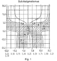
- Fig. 1 shows the starting target astigmatism distribution starting from a given starting area for an addition of 2.5 dpt.
- the maximum astigmatism for the periphery is 2.6 dpt.
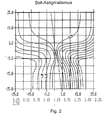
- an interpolation of the target astigmatism values between the 0.5 dd base target isoastigmatism line and the periphery of the spectacle lens is carried out taking into account the maximum temporal astigmatism multiplied by the factor k .
- the interpolation takes place after the in DE 10 2009 005 206 or DE 10 2009 005 214 described truncated cone model for the peripheral target astigmatism.
- multiplication has the maximum temporal astigmatism factor k does not affect the 0.5 dd base target isoastigmatism line.
- the target astigmatism values between the main line and the 0.5 dd base target isoastigmatism line thus remain unchanged.
- Fig. 2 shows the target astigmatism distribution, which is obtained after multiplication of the maximum temporal astigmatism and a subsequent interpolation.
- Asymmetrical target astigmatism distribution shown applies to a progressive lens with an addition of 2.5 dpt.
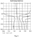
- the total astigmatism specification resulting from a multiplication of the maximum temporal target astigmatism with subsequent interpolation of the target astigmatism values could be scaled in dependence on the addition as a whole in order to obtain target astigmatism specifications for another addition.
- the additional distribution of target astigmatism, which is additionally scaled as a function of the addition, is in Fig. 3 shown.
- Fig. 4 shows a comparative example of a target astigmatism distribution, which consists of the in Fig. 1 shown target astigmatism distribution by means of a (global) scaling depending on the addition (as in DE 10 2008 015 189 described) is obtained.
- This in Fig. 4 The example shown corresponds to a rescaling of the starting nominal astigmatism distribution from the original addition of 2.5 dpt to a new addition of 0.75 dpt.
- Fig. 5 shows a portion of a graphical user interface that allows to set the pre-factor v .
- the tilt angle which corresponds approximately to the frame disc angle for flat base curves, is 5 °.
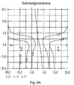
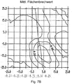
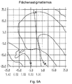
- FIGS. 7A to 10A show the surface properties of the progressive surface of a spectacle lens, which after the in Fig. 6A shown symmetrical Sollastigmatismusvorine has been optimized.
- FIGS. 7B to 10B show the surface properties of the progressive surface of a spectacle lens, which after the in Fig. 6B shown asymmetric, manipulated target specifications has been optimized.
- Fig. 11A , B and 12A, B respectively show the astigmatism ( Fig. 11A . B ) and the refractive power ( Fig. 12A . B ) in the use position of the respective progressive spectacle lens.
- Table 1 summarizes the in the FIGS. 6A , B to 12A, B together target specifications and properties of an optimized according to the respective target specifications progressive area together.
- the progressive surface of the spectacle lens which according to the in Fig. 6B shown manipulated target specifications has been optimized, temporally significantly lower surface refractive index changes (see also Fig. 8A and Fig. 8B ). So is in a comparison of in Fig. 8A and Fig. 8B shown gradient of the surface refractive power of the progressive surface clearly recognize that the optimized according to the manipulated Sollastigmatismusvor protein progressive surface temporally at the same point has significantly lower gradients than the optimized surface according to the symmetrical Sollastigmatismusvor inter. The gradients are smaller by a factor of 5 in this example.
- the use position properties (astigmatism and refractive power in the position of use) of the spectacle lens optimized according to the manipulated target astigmatism specifications are significantly less gradient, with the central visual areas not differing substantially in their size and usability.
- the gradients change from 0.45 dpt / mm to 0.05 dpt / mm.
- a reduction of 0.55 dpt / mm (cf. Fig. 12A ) to 0.15 dpt / mm (cf. Fig. 12B ) be achieved.
- the calculation or optimization of the spectacle lens 10 takes place completely in the position of use of the spectacle lens 12, ie taking into account the predetermined arrangement of the spectacle lens in front of the eyes 12 of the spectacle wearer (defined by the corneal vertex distance, pretilt, etc.) and a predetermined object distance model.
- the object distance model may include the specification of an object area 14, which defines different object distances or object areas for foveal vision.
- the object surface 14 is preferably defined by specifying the reciprocal object distance (the reciprocal object distance) A 1 ( x , y ) along the object-side principal rays.
- a point on the object surface is imaged by the spectacle lens on the remote ball, as in FIG. 13A and 13B shown schematically. At the in Figs. 13A and 13B As shown, the eye-side surface of the spectacle lens 10 is the progressive surface to be optimized.
- the object distance function A 1 ( y ) is represented as the sum of two double asymptotic functions.
- Figs. 14A and 14B show an exemplary starting distance function A 1 G ( y ) (dashed line) and a transformed, adapted to the new object distances object distance function A 1 ( y ) (solid line), which by means of a superposition of the start-distance function A 1 ( y ) with a correction function A 1 Korr ( y ) (dashed line) is obtained.
- the distance and near reference object distances for a particular wearer of glasses or for other designs and applications may differ from the standard model above.
- an object distance of -400 cm in the distance reference point DF and an object distance of -50 cm in the near reference point can be taken into account.
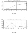
- Fig. 15A shows another exemplary start-to-object distance function A 1 G ( y ) .
- Fig. 15B shows the slope of the start distance function (ie, the derivative of the start distance function after y ).
- the start-to-object distance function has a very smooth transition from the far to the near part.
- the start-object distance function thus describes a hose design for a near-vision glass.
- Fig. 15C shows an exemplary Gaussian function A 1 Gauss ( y ) (ie, the corrective reciprocal object distance along the main line of sight), which can be used, for example, to modify the design characteristic.
- Fig. 15D shows the slope (first derivative to y ) of in Fig. 15C shown Gauss bell curve.
- Fig. 15E shows an object distance function A 1 ( y ) (ie the modified reciprocal object distance along the main line of sight), which is indicated by a Overlay the in Fig. 15A shown starting distance function with the in Fig. 15C Gaussian function shown is obtained.
- Fig. 15F shows the slope (the first derivative after y ) of the in Fig. 15E shown object distance function A 1 ( y ) .
- a modified object distance function which is particularly suitable for a workstation eyeglass lens design.
- Fig. 15H shows the slope (derivative to y ) of in Fig. 15G shown, modified object distance function A 1 new ( y ) .
- the graphical user interface may further include a section (not in FIG Fig. 16A ), which has fields for input and, if necessary, modification of the coefficients of the start-distance function.
- Fig. 16C shows a graphical user interface with a section which is designed to visualize the object distance function composed by superimposition of the start distance function with the correction function.
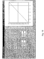
- Fig. 18 and 19 each show an exemplary mask or an exemplary graphical user interface for indicating and optionally changing the parameters of the object distance function and for visualizing the object distance function calculated in this way.
Description
Aspekte der vorliegenden Erfindung betreffen computerimplementierte Verfahren zum Optimieren und Herstellen eines progressiven Brillenglases, entsprechende Vorrichtungen zum Optimieren und zum Herstellen eines progressiven Brillenglases, entsprechende Computerprogrammerzeugnisse und Speichermedien.Aspects of the present invention relate to computer-implemented methods for optimizing and manufacturing a progressive spectacle lens, to corresponding devices for optimizing and producing a progressive spectacle lens, to corresponding computer program products and to storage media.
Eine Optimierung eines progressiven Brillenglases erfolgt in der Regel durch Minimierung einer Zielfunktion, in welcher Ziel- bzw. Sollwerte für zumindest eine optische Größe, z.B. Astigmatismus und/oder Brechkraft, oder Ziel- bzw. Sollwerte für zumindest einen Abbildungsfehler, z.B. astigmatischer Fehler und/oder Refraktionsfehler, des progressiven Brillenglases eingehen. Bei der Optimierung des Brillenglases können die individuellen Verordnungswerte (sph, Zyl, Achse, Add, Prisma, Basis), Parameter der individuellen Lage bzw. Anordnung des Brillenglases vor dem Auge des Brillenträgers (z.B. Hornhautscheitelabstand (HSA), Fassungsscheibenwinkel (FSW), Vorneigung bzw. pantoskopischer Winkel), physiologische Parameter (z.B. Pupillendistanz) berücksichtigt werden. Das progressive Brillenglas kann "online" nach Bestelleingang als Unikat optimiert und berechnet werden.Optimization of a progressive spectacle lens is usually accomplished by minimizing a target function in which target values for at least one optical variable, e.g. Astigmatism and / or refractive power, or target values for at least one aberration, e.g. astigmatic error and / or refractive error, the progressive spectacle lens. When optimizing the spectacle lens, the individual prescription values (sph, cyl, axis, add, prism, base), parameters of the individual position or arrangement of the spectacle lens in front of the wearer's eye (eg corneal vertex distance (HSA), lens angle (FSW), pretilt or pantoscopic angle), physiological parameters (eg pupillary distance) are taken into account. The progressive spectacle lens can be optimized and calculated "online" after ordering as a unique item.
In
Diese Aufgabe wird durch ein computerimplementiertes Verfahren zum Optimieren eines progressiven Brillenglases mit den Merkmalen des Anspruchs 1, ein Computerprogrammerzeugnis mit den Merkmalen des Anspruchs7, ein Speichermedium mit darauf gespeichertem Computerprogramm mit den Merkmalen des Anspruchs 8, eine Vorrichtung zum Optimieren eines progressiven Brillenglases mit dem Merkmalen des Anspruchs 9, ein Verfahren zum Herstellen eines progressiven Brillenglases mit dem Merkmalen des Anspruchs 10 und eine Vorrichtung zum Herstellen eines progressiven Brillenglases mit dem Merkmalen des Anspruchs 11 gelöst.This object is achieved by a computer-implemented method for optimizing a progressive spectacle lens having the features of
Wie bereits oben ausgeführt erfolgt die Optimierung von progressiven Brillengläsern in der Regel durch Minimierung einer Zielfunktion, in welcher Ziel- bzw. Sollwerte für zumindest eine optische Größe (z.B. Astigmatismus und/oder Brechkraft) oder Ziel- bzw. Sollwerte für zumindest einen Abbildungsfehler (z.B. astigmatischer Fehler bzw. astigmatische Abweichung und/oder Refraktionsfehler) des progressiven Brillenglases eingehen. Die in die Zielfunktion eingehenden Ziel- bzw. Sollwerte der zumindest einen optischen Eigenschaft oder des zumindest einen Abbildungsfehlers charakterisieren das Design eines Brillenglases. Darüber hinaus kann das Brillenglasdesign ein geeignetes Objektabstandsmodell umfassen. Das Objektabstandsmodell kann beispielsweise eine Objektabstandsfunktion, welche als der reziproke Objektabstand entlang der Hauptblicklinie definiert ist, umfassen. Ein standardisiertes Objektabstandsmodel ist z.B. in DIN 58 208 Teil 2 (vgl. Bild 6) angegeben. Das Objektabstandsmodel kann jedoch von diesem standardisierten Objektabstandsmodel abweichen.As already explained above, the optimization of progressive spectacle lenses is generally carried out by minimizing a target function in which target values for at least one optical variable (eg astigmatism and / or refractive power) or target values for at least one aberration (eg astigmatic error or astigmatic deviation and / or refractive error) of the progressive spectacle lens. The target values or target values of the at least one optical property or of the at least one aberration that enter the target function characterize the design of a spectacle lens. In addition, the eyeglass lens design may include a suitable object distance model. For example, the object distance model may include an object distance function defined as the reciprocal object distance along the main line of sight. A standardized object distance model is e.g. in DIN 58 208 Part 2 (see Figure 6). However, the object distance model may differ from this standard object distance model.
Unter einer Hauptblicklinie wird die Folge der Durchstoßpunkte der Hauptstrahlen durch die jeweilige Brillenglasfläche beim Blick auf eine Linie verstanden, welche in der senkrechten Ebene liegt, welche den Abstand der beiden Augendrehpunkte halbiert (sog. Zyklopenaugenebene). Bei der Brillenglasfläche kann es sich um die objekt- oder die augenseitige Fläche handeln. Die Lage der Linie in der Zyklopenaugenebene wird durch das gewählte Objektabstandmodell bestimmt.A main line of vision is the sequence of puncture points of the main rays through the respective lens surface when looking at a line which lies in the vertical plane, which halves the distance between the two eye rotation points (so-called cyclopenoid plane). The spectacle lens surface may be the object or the eye-side surface. The position of the line in the cyclops-eye plane is determined by the selected object distance model.
Unter einer Hauptlinie wird eine im Wesentlichen gerade oder gewunden verlaufende Linie verstanden, entlang welcher die gewünschte Zunahme des Brechwerts des Brillenglases vom Fern- zum Nahteil erreicht wird. Die Hauptlinie verläuft im Wesentlichen mittig zu dem Brillenglas von oben nach unten, d.h. entlang einer im Wesentlichen vertikalen Richtung. Die Hauptlinie stellt somit eine Konstruktionslinie im Koordinatensystem der zu optimierenden objektseitigen oder augenseitigen Fläche zur Beschreibung der Sollwerte dar. Der Verlauf der Hauptlinie des Brillenglases wird so gewählt, dass sie zumindest in etwa der Hauptblicklinie folgt. Ein Verfahren zum Anpassen der Hauptlinie an die Hauptblicklinie wird z.B. in
Die Objektabstandsfunktion (d.h. der reziproke Objektabstand an der Hauptblicklinie) spielt eine wesentliche Rolle bei der Designfestlegung und Optimierung von progressiven Brillengläsern. So wird nach dem Satz von Minkwitz bei weitestgehender Vollkorrektion die Grundcharakteristik eines progressiven Brillenglases in der Umgebung der Hauptblicklinie vorwiegend durch den Verlauf der Objektabstandsfunktion A 1(y) entlang der Hauptblicklinie bestimmt.The object distance function (ie the reciprocal object distance at the main line of sight) plays an essential role in the design specification and optimization of progressive spectacle lenses. Thus, according to Minkwitz's theorem, as far as possible full correction is concerned, the basic characteristic of a progressive spectacle lens in the vicinity of the main line of sight is predominantly determined by the course of the object distance function A 1 ( y ) along the main line of vision.
Eine Aufgabe der Erfindung ist es daher, ein effizientes und schnelles Verfahren zu einer automatischen Anpassung der Objektabstandsfunktion an veränderte Objektabstände oder an ein verändertes Objektabstandsmodell bereitzustellen.It is therefore an object of the invention to provide an efficient and rapid method for automatically adapting the object distance function to changed object distances or to a changed object distance model.
Gemäß einem ersten Aspekt der Erfindung wird ein computerimplementiertes Verfahren zum Optimieren eines progressiven Brillenglases vorgeschlagen, wobei das Verfahren die Schritte:
- Vorgeben einer Start-Objektabstandsfunktion A 1G (y),
- Predefining a start distance function A 1 G ( y ),
Erfassen von Objektentfernungsdaten, wobei die Objektentfernungsdaten eine Objektentfernung in zumindest einem vorgegebenen Punkt auf der Hauptblicklinie umfassen;
Abändern oder Transformieren der Start-Objektabstandsfunktion in Abhängigkeit von den erfassten Objektentfernungsdaten; und
Optimieren des progressiven Brillenglases, wobei bei der Optimierung des Brillenglases die abgeänderte/transformierte Objektabstandsfunktion berücksichtigt wird,
umfasst.Acquiring an object distance data, the object distance data including an object distance in at least one predetermined point on the main view line;
Modifying or transforming the start-to-space distance function in response to the acquired object range data; and
Optimizing the progressive spectacle lens, wherein the modified / transformed object distance function is taken into account in the optimization of the spectacle lens,
includes.
Das Abändern/Transformieren der Start-Objektabstandsfunktion A 1G (y) umfasst ein Überlagern der Start-Objektabstandsfunktion A 1G (y) mit einer Korrekturfunktion A 1Korr (y): ![]()
![]()
Die Objektabstandsfunktion gibt den reziproken Objektabstand (die reziproke Objektentfernung) entlang der Hauptblicklinie als Funktion der vertikalen Koordinate y wieder. Anders ausgedrückt ist die Objektabstandsfunktion als der reziproke Objektabstand (die reziproke Objektentfernung) entlang der Hauptblicklinie definiert.The object distance function represents the reciprocal object distance (the reciprocal object distance) along the main line of sight as a function of the vertical coordinate y . In other words, the object distance function is defined as the reciprocal object distance (the reciprocal object distance) along the main line of sight.
Die Korrekturfunktion weist zumindest einen variablen Parameter auf, welcher derart in Abhängigkeit von den erfassten Objektentfernungsdaten bestimmt wird, dass der Wert der abgeänderten Start-Objektabstandsfunktion in zumindest einem vorgegebenen Punkt gleich dem reziproken Wert der erfassten Sollobjektentfernung für diesen Punkt ist. Mit anderen Worten wird der zumindest eine variable Parameter (Koeffizient) der Korrekturfunktion derart in Abhängigkeit von den erfassten Objektabstandsdaten bestimmt oder festgelegt, dass die Bedingung: ![]()
![]()
erfüllt wird, wobei in der obigen Formel:
- A 1D den reziproken Wert der erfassten Sollobjektentfernung bzw. des erfassten Sollobjektabstands in dem zumindest einen vorgegebenen Punkt D auf der Hauptblicklinie, wobei der Punkt D eine vertikale Koordinate yD aufweist; und A1 (y=yD ) den Wert der Objektabstandsfunktion A1 (y) im vorgegebenen Punkt D auf der Hauptblicklinie bezeichnen.
- A 1 D is the reciprocal of the detected solar object distance and the detected solar object distance, respectively, in the at least one predetermined point D on the main line of sight, the point D having a vertical coordinate y D ; and A 1 ( y = y D ) denote the value of the object distance function A 1 ( y ) at the predetermined point D on the main line of sight.
Dabei kann das Koordinatensystem ein beliebiges Koordinatensystem sein, insbesondere eines der zuvor beschriebenen Koordinatensysteme {x,y} oder {u, y}, wobei u den Abstand von der Hauptblicklinie oder Hauptlinie darstellt. In einem Koordinatensystem {x, y} gilt für die Punkte auf der Hauptblicklinie (x = xHBL = x 0 , y). In einem Koordinatensystem {u, y} der Hauptblicklinie gilt für die Punkte auf der Hauptblicklinie (u = 0, y). In this case, the coordinate system can be any coordinate system, in particular one of the previously described coordinate systems { x , y } or { u, y }, where u represents the distance from the main sight line or main line. In a coordinate system { x , y }, the points on the main view line ( x = x HBL = x 0 , y ) apply . In a coordinate system { u, y } of the main line of sight applies to the points on the main sight line ( u = 0, y ) .
Vorzugsweise umfassen die Objektentfernungsdaten zumindest eine Sollobjektentfernung A 1Ferne in einem vorgegeben Fernbezugspunkt (Designpunkt Ferne) DF auf der Hauptblicklinie und eine Sollobjektentfernung A 1Nähe in einem vorgegebenen Nahbezugspunkt (Designpunkt Nähe) DN auf der Hauptblicklinie. Der zumindest eine variable Parameter der Korrekturfunktion wird derart bestimmt oder festgelegt, dass der jeweilige Wert der abgeänderten Start-Objektabstandsfunktion im Fern- und/oder Nahbezugspunkt gleich dem entsprechenden reziproken Wert der erfassten Sollobjektentfernung für den Fern- und/oder Nahbezugspunkt ist.Preferably, the object removal data comprises at least one Solobject distance A 1 Distance in a given distance reference point (design point distance) DF on the main sight line and a sol object distance A 1 Proximity in a given near reference point (design point proximity) DN on the main sight line. The at least one variable parameter of the correction function is determined or determined in such a way that the respective value of the modified start-distance function at the far and / or near reference point is equal to the corresponding reciprocal value of the detected target distance for the far and / or near reference point.
Anders ausgedrückt umfassen in diesem Fall die Objektentfernungsdaten eine Sollobjektentfernung für den Fernbezugspunkt DF und eine Sollobjektentfernung für den Nahbezugspunkt DN. Der Fernbezugspunkt befindet sich auf der Hauptblicklinie auf einer vertikalen Höhe yDF. Der Nahbezugspunkt befindet sich auf der Hauptblicklinie auf einer vertikalen Höhe yDN. Der zumindest eine variable Parameter der Korrekturfunktion wird derart festgelegt, dass die Bedingungen: 
- A 1Ferne den reziproken Wert der Sollobjektentfernung im Fernbezugspunkt DF, und
- A 1Nähe den reziproken Wert der Sollobjektentfernung im Nahbezugspunkt DN, bezeichnen.
- A 1 Removes the reciprocal of the solar object distance at the distance reference DF , and
- A 1 Near the reciprocal of the solar object distance in the near reference point DN .
Die Start-Objektabstandsfunktion, nachfolgend auch Grund-Objektabstandsfunktion oder Grundfunktion genannt, A 1G (y)=A 1G (x=x0 ,y)=A 1G (u-0,y) kann eine beliebige analytische Funktion oder auch eine Interpolationsfunktion (z.B. Splinefunktion) sein. Ebenfalls kann A 1G (y) punktweise vorgegeben werden.The starting object distance function, also referred to below as the basic object distance function or basic function, A 1 G ( y ) = A 1 G ( x = x 0 , y ) = A 1 G ( u- 0, y ) can be any analytical function or be an interpolation function (eg spline function). Likewise, A 1 G ( y ) can be specified point by point.
Die Start-Objektabstandsfunktion kann beispielsweise analytisch mittels einer Doppelasymptotenfunktion der Form: 
Eine Doppelasymptotenfunktion weist insbesondere folgende vorteilhafte Eigenschaften auf:
- Die beiden Asymptoten nehmen jeweils entsprechend die Werte bG und (bG +aG ) an;
- Mit dem variablen Parameter d kann die vertikale Position gesteuert werden. Vorzugsweise liegt der Parameter d im Bereich -10 < d < 10, weiter bevorzugt im Bereich -8 < d < 5;
- Je größer der Betrag des variablen Parameters c desto schneller erfolgt der Übergang von einer zur anderen Asymptote. Der Parameter c wird vorzugsweise derart ausgewählt, dass |c| < 1,5;
- Der Parameter m (m > 0) beschreibt die Asymmetrie der Funktion. Bei m=1 weist die Doppelasymptotenfunktion eine Punktsymmetrie mit Zentrum y=-d auf. Vorzugsweise liegt der Parameter m im Bereich0,2 < m< 2, weiter
bevorzugt im Bereich - Wird für den variablen Parameter c das negative Vorzeichen (c < 0) gewählt, so gilt:
- Nahteilasymptote A 1G (y→-∞)=A 1GNähe =bG ; und
- Fernteilasymptote A 1G (y→+∞)=A 1Ferne =(bG +aG ).
- The two asymptotes respectively assume the values b G and ( b G + a G );
- The variable parameter d can be used to control the vertical position. The parameter d is preferably in the range -10 < d <10, more preferably in the range -8 < d <5;
- The larger the amount of variable parameter c, the faster the transition from one to the other asymptote occurs. The parameter c is preferably selected such that | c | <1.5;
- The parameter m ( m > 0) describes the asymmetry of the function. At m = 1 the double asymptotic function shows a point symmetry with center y = -d . The parameter m is preferably in the range 0.2 < m <2, more preferably in the range 0.4 < m <1;
- If the negative sign ( c <0) is selected for the variable parameter c, the following applies:
- Nahteilasymptote A 1 G ( y → -∞) = A 1 GNear = b G ; and
- Fernteilasymptote A 1 G ( y → + ∞) = A 1 distance = ( b G + a G ) .
In der Regel wird die Start-Objektabstandsfunktion A 1G (y), welche dem Startdesign (Grunddesign) zugeordnet ist, derart vorgegeben, dass die Objektentfernungen im Fernbezugspunkt DF und im Nahbezugspunkt DN (Designpunkten Ferne und Nähe) in etwa den Standardobjektentfernungen A 1GFerne und A 1GNähe , d.h. die Sollobjektentfernungen in dem Fern- und dem Nahbezugspunkt gemäß einem Standard-Objektabstandsmodell, entsprechen. Die Parameter aG,bG können folglich anhand den Standardvorgaben für die reziproken Objektabstände A 1GFerne und A 1GNähe in den Fern- und Nahbezugspunkte DF und DN automatisch ermittelt werden. Ein Standard-Objektabstandsmodell ist z.B. in DIN 58 208 Teil 2 angegeben.In general, the starting distance function A 1 G ( y ), which is the starting design (Basic design), given such that the object distances at the distance reference point DF and in the near reference point DN (design points distance and proximity) are approximately the standard object distances A 1 F and A 1 G , ie, the lens object distances in the far and near reference points according to a standard Object distance model. The parameters a G , b G can therefore be determined automatically in the distance and near reference points DF and DN using the standard specifications for the reciprocal object distances A 1 GFerne and A 1 GN . A standard object distance model is specified, for example, in DIN 58 208
Wählt ein Brillenträger in dem Fern- und/oder Nahbezugspunkt abweichende Objektentfernungen A 1Ferne und A 1Nähe wird die Start-Objektabstandsfunktion mit einer Korrekturfunktion überlagert, um dieser Veränderung Rechnung zu tragen.If an eyeglass wearer chooses different object distances A 1 distance and A 1 proximity in the distance and / or near reference point, the start object distance function is superimposed with a correction function in order to take this change into account.
Die Korrekturfunktion A 1Korr (y) ist.
- eine Doppelasymptotenfunktion der Form

- eine lineare Funktion der Start-Objektabstandsfunktion A 1Korr (y)=c+mA 1G (y) mit den Parametern (Koeffizienten) c und m.
- a double asymptotic function of the form
- a linear function of the starting distance function A 1 Korr ( y ) = c + mA 1 G ( y ) with the parameters (coefficients) c and m.
Zusätzlich kann die Start-Objektabstandsfunktion mit anderen Funktionen überlagert werden, um z.B. eine gezielte Abänderung der Designcharakteristik zu erzielen. So kann die Start-Objektabstandsfunktion mit einer Funktion in Form einer Gauss'schen Glockenkurve ![]()
![]()
Zumindest einer der Parameter der Korrekturfunktion ist variabel und wird in Abhängigkeit von den erfassten Objektabstandsdaten, insbesondere von den geänderten Sollwerten für die Objektabstände im Fern- und/oder im Nahbezugspunkt bestimmt bzw. festgelegt.At least one of the parameters of the correction function is variable and is included in Dependent on the detected object distance data, in particular determined or fixed by the changed setpoint values for the object distances in the far and / or near reference point.
Vorzugsweise ist die Korrekturfunktion eine Doppelasymptotenfunktion der Form ![]()
![]()
In diesem Fall gilt: 
Die variablen Parameter/Koeffizienten bkorr und akorr der Korrekturfunktion werden in Abhängigkeit von den erfassten Objektentfernungsdaten bestimmt bzw. festgelegt.The variable parameters / coefficients b corr and a corr of the correction function are determined or established as a function of the acquired object distance data.
Vorzugsweise sind sowohl die Start-Objektabstandsfunktion als auch die Korrekturfunktion Doppelasymptotenfunktionen. Vorzugsweise weist die Korrekturfunktion die gleichen Parameter c, d und m auf, wie die Parameter der Start-Objektabstandsfunktion (d.h.c=ckorr,d=dkorr,m=mkorr ). In diesem Fall gilt: 
Somit kann sichergestellt werden, dass die Charakteristik der Start-Objektabstandsfunktion bei einer Anpassung an geänderte Objektabstände im Wesentlichen beibehalten wird.Thus it can be ensured that the characteristics of the Start object distance function is substantially maintained when adjusting to changed object distances.
Mit den beiden Bedingungen A 1(yD
Die Koeffizienten/Parameter der Start-Objektabstandsfunktion (Grundfunktion) und die Koeffizienten/Parameter der Korrekturfunktion können vorab bestimmt werden und vorzugsweise getrennt in einem Speicher als Datenfiles gespeichert werden. Dies ermöglicht eine einfache nachträgliche Reproduktion und Änderung der Werte des Startdesigns.The coefficients / parameters of the starting distance function (basic function) and the coefficients / parameters of the correction function can be determined beforehand and preferably stored separately in a memory as data files. This allows easy subsequent reproduction and modification of the values of the startup design.
Wie bereits oben ausgeführt, kann die Start-Objektabstandsfunktion, welche insbesondere eine Doppelasymptotenfunktion sein kann, zusätzlich zu einer Überlagerung mit einer Korrekturfunktion A 1Korr (y) - mit einer Funktion in Form einer Gauss'schen Glockenkurve ![]()

![]()
In dem Fall, dass die Start-Objektabstandsfunktion eine Doppelasymptotenfunktion ist, gilt: 
Durch die Überlagerung der Start-Objektabstandsfunktion (Grundfunktion) mit einer Gauss'schen Glockenkurve (Gauss'schen Funktion) kann die Kurvencharakteristik der Start-Objektabstandsfunktion gezielt abgeändert werden. Insbesondere bewirkt die Gauss'sche Funktion, dass die Objektabstandsfunktion oberhalb des Gaussmaximums flacher verläuft. Die Brechwertänderung wird in diesem Bereich geringer, die Isoastigmatismuslinien rücken weiter nach außen und der im Wesentlichen fehlerfreie Glasbereich, z.B. der Glasbereich mit einem astigmatischen Fehler kleiner als 0,5 dpt, wird breiter. Somit können Bereiche (z.B. der Zwischenbereich) gezielt höher oder niedriger gewichtet werden.By overlaying the start-object distance function (basic function) with a Gaussian bell curve (Gaussian function), the curve characteristic of the start-object distance function can be modified in a targeted manner. In particular, the Gaussian function causes the object distance function to be flatter above the gauss maximum. The refractive index change is reduced in this range, the isoastigmatism lines move farther outward and the substantially defect-free glass region, e.g. the glass area with an astigmatic error smaller than 0.5 D becomes wider. Thus, areas (e.g., the intermediate area) may be weighted higher or lower in a targeted manner.
So kann zum Beispiel aus einem gleichmäßigen, langsamen Übergang vom Fernteilwert der Objektentfernung A 1GFerne zum Nahteilwert der Objektentfernung A 1GNähe (gb ≈ 0) ein anderer Verlauf der Objektabstandsfunktion A 1(u=0,y)=A 1(y)(A 1-Verlauf) für ein Bildschirmarbeitsplatzglas (gb≠0, σ≠0) erzeugt werden.Thus, for example, a uniform, slow transition from the distance portion value of the object distance A 1 GFerne to Nahteilwert the object distance A 1 GNähe (g b ≈ 0) a different course of the object distance function A 1 (u = 0, y) = A 1 (y) ( A 1 -pass) for a VDU workstation glass ( g b ≠ 0 , σ ≠ 0) are generated.
In einem Beispiel kann anhand einer prozentualen Gewichtung gG der Gauss'schen Funktion, wobei gG ∈ [0,100]%, nach Vorgabe eines maximalen A 1-Zuwachses der Gauss'schen Funktion g bmax (eine designspezifische Vorgabe) der zugehörige Koeffizient gb der Gauss'schen Funktion ermittelt werden: 
Bei einer 90% Gewichtung der Gauss'schen Funktion und einem maximalen A 1-Zuwachs der Gauss'schen Funktion g bmax = 0,6 dpt ergibt sich für gb z.B. einen Wert von 0,54 dpt.With a 90% weighting of the Gaussian function and a maximum A 1 gain of the Gaussian function g b max = 0.6 d, a value of 0.54 dpt results for g b, for example.
Die prozentuale Gewichtung gG sowie die weiteren Koeffizienten der Gauss'schen Funktion können für das jeweilige Grunddesign vorgegeben werden oder z.B. anhand des in
Die Überlagerung der Start-Objektabstandsfunktion mit einer Gauss'schen Glockenkurve kann gemäß einem weiteren Aspekt unabhängig von einer Überlagerung mit einer Korrekturfunktion erfolgen.The superimposition of the start-distance function with a Gaussian bell curve can, according to a further aspect, take place independently of an overlay with a correction function.
Gemäß einem weiteren Beispiel ist die Korrekturfunktion AKorr (y) eine lineare Funktion der Start-Objektabstandsfunktion: 
Die abgeänderte Objektabstandsfunktion stellt somit ebenfalls eine lineare Funktion der Start-Objektabstandsfunktion A 1G (u=0,y)=A 1G (y) dar: ![]()
![]()
![]()
![]()
Vorzugsweise werden die Geradenkoeffizienten c und m aus den Abweichungen der Werte der Start-Objektabstandsfunktion A 1G(y) von den erfassten Sollwerten der reziproken Objektentfernung in dem Fern- und Nahbezugspunkt berechnet. Anders ausgedrückt erfolgt eine lineare Anpassung der Start-Objektabstandsfunktion an die geänderten Objektabstände im Fern- und/oder im Nahbezugspunkt.Preferably, the straight line coefficients c and m are calculated from the deviations of the values of the start distance function A 1G ( y ) from the detected set points of the reciprocal distance in the far and near reference points. In other words, there is a linear adaptation of the start-distance function to the changed object distances in the far and / or in the near reference point.
Vorzugsweise gilt In diesem Fall gilt für den Koeffizienten c und m: 
![]()
![]()
- A 1Ferne den reziproken Wert der Sollobjektentfernung im Fernbezugspunkt;
- A 1Nähe den reziproken Wert der Sollobjektentfernung im Nahbezugspunkt; Nähe;
- yF die vertikale Koordinate des Fernbezugspunkts; und
- yN die vertikale Koordinate des Nahbezugspunkts
- A 1 distance the reciprocal value of the target object distance in the distance reference point;
- A 1 proximity the reciprocal of the solar object distance in the near reference point; close;
- y F is the vertical coordinate of the distance reference point; and
- y N is the vertical coordinate of the near reference point
Die Geradenkoeffizienten c und m werden beispielsweise wie folgt berechnet:
- In einem ersten Schritt werden die Abweichungen der Werte der Start-Objektabstandsfunktion A 1G (y) in den Bezugs- bzw. Designpunkten DF (mit den Koordinaten (x=x 0,yDF )=(u=0,yDF )) und DN (mit den Koordinaten (x=x0,yDN )=(u=0,yDN )) von den entsprechenden (individuellen) Werten A 1Ferne und A 1Nähe des reziproken Sollobjektanstands (der reziproken Sollobjektentfernung) für diese Punkten ermittelt:

- In a first step, the deviations of the values of the start distance function A 1 G ( y ) in the reference or design points DF (with the coordinates (x = x 0 , y DF ) = ( u = 0 , y DF )) and DN (with the coordinates ( x = x 0 , y DN ) = ( u = 0, y DN )) of the corresponding (individual) values A 1 distance and A 1 proximity of the reciprocal solar object distance (the reciprocal solar object distance) for these points determined:
Die Geradenkoeffizienten c und m können aus den zuvor ermittelten Abweichungen wie folgt berechnet werden: 
In den obigen Formeln bezeichnen:
- A 1G(y) die Start-Objektabstandsfunktion;
- A 1Ferne den Sollwert des reziproken Objektabstandes im Fernbezugspunkt (Designpunkt Ferne);
- A 1Nähe den Sollwert des reziproken Objektabstandes im Nahbezugspunkt (Designpunkt Nähe); und
- A1 (y) die korrigierte/angepasste Objektabstandsfunktion.
- A 1G ( y ) the start distance function;
- A 1 distance the target value of the reciprocal of object distance in the distance reference point (design point distance);
- A 1 proximity the target value of the reciprocal object distance in the near reference point (design point proximity); and
- A 1 ( y ) the corrected / adjusted object distance function.
Durch diese angepasste Objektabstandsfunktion, welche eine lineare Funktion der Start-Objektabstandsfunktion ist, wird der Verlauf des reziproken Objektabstandes entlang der Hauptblicklinie nicht wesentlich geändert. Insbesondere unterscheiden sich die Steigungen bzw. Ableitungen der Grundfunktion A 1G (y) und der abgeänderten/korrigierten Objektabstandsfunktion A 1(y) lediglich um den konstanten Faktor (1 + m) : 
Anders ausgedrückt wird die erste Ableitung der Start-Objektabstandsfunktion nur um einen Faktor (1+m) verändert. Bei weitestgehender Vollkorrektion wird die Grundcharakteristik eines progressiven Brillenglases in der Umgebung der Hauptblicklinie jedoch vorwiegend durch den Verlauf der Objektabstandsfunktion A 1(y) entlang der Hauptblicklinie bestimmt (Satz von Minkwitz). Die lineare Anpassung der Start-Objektabstandsfunktion ermöglicht es, die Designcharakteristik auch bei einer Anpassung der Objektabstände an geänderte Vorgaben in einem oder zwei Punkten mit vernachlässigbarem Rechenaufwand sehr gut zu erhalten.In other words, the first derivative of the starting distance function is only changed by a factor (1 + m ). However, as much as possible full correction, the basic characteristic of a progressive spectacle lens in the vicinity of the main sight line becomes predominantly due to the course of the object distance function A 1 ( y ) determined along the main line of sight (Minkwitz's theorem). The linear adaptation of the start-object distance function makes it possible to obtain the design characteristic very well even with an adaptation of the object distances to changed specifications in one or two points with negligible computation effort.
Das oben beschriebene Verfahren lässt sich unabhängig vom Verlauf des reziproken Objektabstandes entlang der Hauptblicklinie anwenden. Ebenfalls ist es möglich, die Charakteristik der Objektabstandsfunktion entlang der Hauptblicklinie im Wesentlichen beizubehalten und gleichzeitig die Objektabstände in den Designpunkten/Bezugspunkten designabhängig zu variieren oder an den Bedürfnissen oder Wünschen des Brillenträgers anzupassen.The method described above can be applied independently of the course of the reciprocal object distance along the main sight line. It is also possible to substantially maintain the characteristic of the object distance function along the main line of sight while at the same time design-varying the object distances in the design points / reference points or adapting them to the needs or wishes of the spectacle wearer.
In diesem Beispiel kann die Start-Objektabstandsfunktion (Grundfunktion) A 1G (y) eine beliebige analytische Funktion oder auch eine Interpolationsfunktion (Splinefunktion) sein. Es müssen keine Koeffizienten der Grundfunktion bekannt sein oder abgeändert werden. Wenn A 1G (y) punktweise vorgegeben oder, wie in der Patentanmeldung
Die oben beschriebenen Transformationen der Start-Objektabstandsfunktion durch Überlagerung der Start-Objektanstandsfunktion mit einer Doppelasymptoten-Korrekturfunktion, durch Überlagerung der Start-Objektanstandsfunktion mit einer Gauss'schen Funktion oder durch eine lineare Anpassung können selbstverständlich in beliebiger Reihenfolge miteinander kombiniert werden.The above-described transformations of the start-object distance function by superimposition of the start-object-standby function with a double asymptotic correction function, by superposition of the start-object-standby function with a Gaussian function or by a linear fit can of course be combined in any order.
In einem bevorzugten Beispiel umfasst computerimplementierte Verfahren zum Optimieren eines progressiven Brillenglases ferner die folgenden Schritte:
- Vorgeben einer Start-Sollastigmatismusverteilung AstSoll
start für das progressive Brillenglas; - Ermitteln einer transformierten Sollastigmatismusverteilung AstSoll
neu und - Optimieren des progressiven Brillenglases anhand der transformierten Sollastigmatismusverteilung.
- Specifying a start-target astigmatism distribution Ast Soll
begin for the progressive spectacle lens; - Determining a transformed target astigmatism distribution Ast Soll
New and - Optimizing the progressive spectacle lens based on the transformed target astigmatism distribution.
Das Ermitteln einer transformierten Sollastigmatismusverteilung AstSoll
- Multiplizieren des Werts des maximalen temporalen Sollastigmatismus max_AstSoll_temporalstart der Start-Sollastigmatismusverteilung AstSoll
start mit einem Faktor k:
- wodurch sich ein abgeänderter maximaler temporaler Astigmatismus max_AstSoll_temporalneu ergibt, wobei der Faktor k eine Funktion zumindest eines Verordnungswerts und/oder zumindest eines Parameters des Brillenglases oder dessen Anordnung vor den Augen des Brillenträgers ist; und
- Transformieren der Start-Sollastigmatismusverteilung AstSoll
start auf Basis des abgeänderten maximalen temporalen Astigmatismus max_AstSoll _temporalneu .
- Multiplying the value of the maximum temporal target astigmatism max_ branch target _temporal start of the start target astigmatism distribution Ast Soll
begin with a factor k : - whereby max_ new branch results _temporal a modified maximum temporal astigmatism target, where the factor k is a function of at least one regulation value and / or at least one parameter of the spectacle lens or its arrangement in front of the eyes of the spectacle wearer; and
- Transform the start-target astigmatism distribution Ast Soll
begin based on the modified maximal temporal astigmatism max_ branch Soll _ temporal neu .
Wie bereits oben ausgeführt erfolgt die Optimierung von progressiven Brillengläsern in der Regel durch eine iterative Minimierung einer Zielfunktion, in welcher Ziel- bzw. Sollwerte für zumindest eine optische Größe (z.B. Astigmatismus und/oder Brechkraft) oder Ziel- bzw. Sollwerte für zumindest einen Abbildungsfehler (z.B. astigmatischer Fehler und/oder Refraktionsfehler) des progressiven Brillenglases eingehen. Der Refraktionsfehler stellt die Differenz des Brechwerts des Brillenglases von dem Brechwert, welcher mittels Refraktionsbestimmung ermittelt wird, dar. Der astigmatische Fehler stellt die Differenz des Astigmatismus des Brillenglases von dem Astigmatismus, welcher mittels Refraktionsbestimmung ermittelt wird, dar. Vorzugsweise handelt es sich dabei um Werte in Gebrauchsstellung des Brillenglases, d.h. unter Berücksichtigung des Systems Brillenglas-Auge. Freiheitsgrad bei der Optimierung der Zielfunktion ist üblicherweise die Pfeilhöhe der Vorder- oder der Rückfläche des Brillenglases oder sowohl der Vorder- als auch der Rückfläche, z.B. bei einem doppelprogressiven Brillenglas.As already explained above, the optimization of progressive spectacle lenses is generally carried out by an iterative minimization of a target function in which target values for at least one optical variable (eg astigmatism and / or refractive power) or target values for at least one aberration (eg astigmatic error and / or refractive error) of the progressive spectacle lens. The refractive error represents the difference of the refractive power of the spectacle lens from the refractive power, which is determined by refraction determination. The astigmatic error represents the difference of the astigmatism of the spectacle lens from The astigmatism, which is determined by means of refraction determination, is. These are preferably values in the position of use of the spectacle lens, ie, taking into account the system spectacle lens-eye. Degree of freedom in the optimization of the objective function is usually the arrow height of the front or the rear surface of the spectacle lens or both the front and the rear surface, for example, in a double-progressive spectacle lens.
Eine designbasierte Optimierung eines progressiven Brillenglases kann zum Beispiel durch Minimierung einer Zielfunktion der Form: 

In den obigen Formeln bezeichnen:
- ΔRi,Soll
- den Sollwert des lokalen Refraktionsfehlers/Brechwerts an der i -ten Bewertungsstelle;
- ΔRi
- den tatsächlichen lokalen Refraktionsfehler/Brechwert an der i -ten Bewertungsstelle;
- Asti,soll
- den Sollwert des lokalen astigmatischen Fehlers/Astigmatismus an der i -ten Bewertungsstelle;
- Asti
- der tatsächliche lokale astigmatische Fehler/Astigmatismus an der i -ten Bewertungsstelle;
- gi,ΔR
- die lokale Gewichtung des Refraktionsfehlers/Brechwert an der i-ten Bewertungsstelle; und
- gi,Ast
- die lokale Gewichtung des astigmatischen Fehlers/Astigmatismus an der i-ten Bewertungsstelle.
- Δ R i, target
- the set point of the local refractive error / refractive power at the i th evaluation point;
- ΔR i
- the actual local refractive error / power at the i th evaluation point;
- Branch i, shall
- the set point of the local astigmatic error / astigmatism at the i th evaluation point;
- Branch i
- the actual local astigmatic error / astigmatism at the i- th evaluation point;
- g i, ΔR
- the local weighting of the refractive error / refractive power at the i- th Assessment body; and
- g i, branch
- the local weighting of the astigmatic error / astigmatism at the i th evaluation point.
Die in die Zielfunktion eingehenden Ist- und Sollwerte der zumindest einen optischen Eigenschaft können sowohl Sollwerte (Flächenwerte oder Werte in Gebrauchstellung) des Brillenglases als auch Sollwerte für zumindest einen Abbildungsfehler sein. Im Sinne dieser Anmeldung wird daher unter dem Begriff "Sollastigmatismus" sowohl der Astigmatismus des Brillenglases (als Flächenbrechwert oder in Gebrauchsstellung) als auch der astigmatische Fehler verstanden. Ebenfalls wird unter dem Begriff "Sollastigmatismusverteilung" im Sinne dieser Anmeldung sowohl die räumliche Verteilung der Sollwerte des Astigmatismus des Brillenglases als auch die räumliche Verteilung der Sollwerte des astigmatischen Fehlers verstanden. Die Sollwerte der zumindest einen optischen Eigenschaft des Brillenglases und insbesondere die Sollwerte des Astigmatismus oder des astigmatischen Fehlers charakterisieren das "Design" eines Brillenglases. Darüber hinaus kann das Brillenglasdesign ein geeignetes Objektabstandsmodell umfassen. Das Objektabstandsmodell kann beispielsweise eine Objektabstandsfunktion, welche als der reziproke Objektabstand entlang der Hauptblicklinie definiert ist, umfassen. Ein standardisiertes Objektabstandsmodel ist z.B. in DIN 58 208 Teil 2 (vgl. Bild 6) angegeben. Das Objektabstandsmodel kann jedoch von diesem standardisierten Objektabstandsmodel abweichen.The actual and desired values of the at least one optical property entering the target function can be setpoints (area values or values in the use position) of the spectacle lens as well as setpoint values for at least one aberration. For the purposes of this application, the term "target astigmatism" is therefore understood to mean both the astigmatism of the spectacle lens (as surface refractive power or in the position of use) and the astigmatic error. Likewise, the term "target astigmatism distribution" in the context of this application means both the spatial distribution of the nominal values of the astigmatism of the spectacle lens and the spatial distribution of the nominal values of the astigmatic error. The nominal values of the at least one optical property of the spectacle lens and in particular the nominal values of the astigmatism or the astigmatic error characterize the "design" of a spectacle lens. In addition, the eyeglass lens design may include a suitable object distance model. For example, the object distance model may include an object distance function defined as the reciprocal object distance along the main line of sight. A standardized object distance model is e.g. in DIN 58 208 Part 2 (see Figure 6). However, the object distance model may differ from this standard object distance model.
Die Sollastigmatismusverteilung, auf deren Basis das progressive Brillenglas optimiert wird, kann mittels einer Transformation eines bestehenden bzw. vorgegebenen Designs (Startdesign, Basisdesign) erhalten werden. So wird z.B. in
Das Startdesign (Basisdesign) weist in der Regel aufgrund der binokularen Abbildungseigenschaften eine annähernd symmetrische Verteilung des Sollastigmatismus in Bezug auf die Hauptblicklinie auf. Bei einer additions- und/oder wirkungs- und/oder progressionslängenabhängigen Transformation des Startdesigns wird die annähernd symmetrische Verteilung des Sollastigmatismus im Wesentlichen beibehalten.The startup design (base design) generally exhibits an approximately symmetrical distribution of the target astigmatism with respect to the main line of sight due to the binocular imaging properties. In the case of an addition and / or action and / or progression-length-dependent transformation of the start design, the approximately symmetrical distribution of the target astigmatism is essentially maintained.
Es ist erkannt worden, dass für bestimmte Kombinationen von Verordnungswerten und/oder Parametern des Brillenglases und/oder dessen Anordnung vor den Augen des Brillenträgers (d.h. dessen Gebrauchsstellung) die oben beschriebene Vorgehensweise, bei welcher die in die Zielfunktion eingehende Sollastigmatismusverteilung annähernd symmetrisch in Bezug auf die Hauptblicklinie ist, zu suboptimalen Ergebnissen führen kann. So sind z.B. die Gradienten der Flächeneigenschaften der progressiven Fläche und/oder die Gradienten der Gebrauchswerte häufig relativ groß. Dies führt zu verschlechterten Gebrauchsstellungseigenschaften des Brillenglases (Astigmatismus und/oder Brechwert in Gebrauchsstellung des Brillenglases).It has been recognized that for certain combinations of prescription values and / or parameters of the spectacle lens and / or its arrangement in front of the spectacle wearer (ie its position of use), the procedure described above, in which the target astigmatism distribution entering the objective function is approximately symmetrical with respect to The main line of vision is that can lead to suboptimal results. Thus, e.g. the gradients of the surface properties of the progressive surface and / or the gradients of the use values are often relatively large. This leads to impaired use position properties of the spectacle lens (astigmatism and / or refractive power in the position of use of the spectacle lens).
Diese Nachteile treten insbesondere bei Brillengläsern mit flacher Basiskurve (d.h. mit einer Basiskurve im Bereich von 0 dpt bis 4 dpt) und höheren Rückflächenkrümmungen (d.h. Rückflächenkrümmungen größer oder gleich -6 dpt) auf, insbesondere in Kombination mit:
- hohen Verordnungszylindern, d.h. Zylindern im Bereich von größer oder gleich 2 dpt, und/oder
- schiefen Achslagen des Verordnungszylinders, d.h. Achslagen
des Verordnungszylinders von 0 bis 90° nach Tabo bei rechten Brillengläsern, und von 90 bis 180° bei linken Brillengläsern; und/oder - geringerer Verordnungsaddition, d.h. eine Addition < 2,0 dpt, vorzugsweise eine Addition ≤ 1,5 dpt,
- high prescription cylinders, ie cylinders in the range greater than or equal to 2 D, and / or
- oblique axial positions of the prescription cylinder, ie axis positions of the prescription cylinder from 0 to 90 ° to Tabo in right-hand lenses, and from 90 to 180 ° in the case of left-hand lenses; and or
- lower prescription addition, ie an addition <2.0 D, preferably an addition ≤ 1.5 d,
Es ist ferner erkannt worden, dass ein Grund für das Auftreten höherer Gradienten der Flächeneigenschaften bei Brillengläsern, welche eine der obigen Kombinationen aufweisen, die symmetrische Verteilung des Sollastigmatismus in Bezug auf die Hauptblicklinie ist. So kann z.B. bei einer torischen Überlagerung einer vorgegebenen Starfläche mit einer torischen oder atorischen Fläche temporal ein astigmatischer Fehler auftreten, welcher teilweise deutlich unter dem Wert des Sollastigmatismus gemäß der symmetrischen Sollastigmatismusverteilung liegt. Der Optimierungsprozess versucht allerdings die symmetrischen Vorgaben für den Sollastigmatismus zu erreichen und "verbiegt" deshalb die zu optimierenden Fläche an dieser Stelle stärker, als dies für niedrige Additionen notwendig wäre.It has also been recognized that a reason for the occurrence of higher gradients of the surface properties in spectacle lenses having any one of the above combinations is the symmetrical distribution of the target astigmatism with respect to the main line of sight. Thus, e.g. in the case of a toric superimposition of a given star area with a toric or atoric surface, an astigmatic error occurs temporally which is in some cases significantly below the value of the target astigmatism according to the symmetrical distribution of target astigmatism. However, the optimization process tries to achieve the symmetric requirements for the target astigmatism and therefore "bends" the surface to be optimized at this point more than would be necessary for low additions.
Vorzugsweise wird daher der temporale Sollastigmatismus in der Peripherie des Brillenglases mit einem Faktor k multipliziert, um diesem Umstand Rechnung zu tragen. Der Faktor k nimmt vorzugsweise den Wert 1 an, wenn keine Manipulation der Sollastigmatismuswerte stattfinden soll und einen Wert kleiner als 1 an, wenn die Sollastigmatismuswerte manipuliert werden sollen. Der Faktor k ist eine Funktion zumindest eines Verordnungswerts (wie z.B. Sphäre, Zylinder, Zylinderachse, Prisma, Prismenbasis und/oder Addition) und/oder zumindest eines Parameters des Brillenglases oder dessen Anordnung vor den Augen des Brillenträgers (d.h. dessen Gebrauchsstellung). Die Parameter des Brillenglases und/oder dessen Anordnung vor den Augen des Brillenträgers (d.h. dessen Gebrauchsstellung) sind beispielsweise der Fassungsscheibenwinkel, der Verkippungswinkel, der Hornhautscheitelabstand (HSA), die Vorneigung oder der pantoskopische Winkel, die Pupillendistanz, der Augendrehpunktabstand und/oder andere Parameter. Es kann sich dabei um durchschnittliche (wie z.B. in DIN 58 208 Teil 2 definiert) oder individuell für einen bestimmten Brillenträger ermittelte Werte handeln.Preferably, therefore, the temporal target astigmatism in the periphery of the spectacle lens is multiplied by a factor k in order to take this circumstance into account. The factor k preferably assumes the
Insbesondere wird vorgeschlagen, den maximalen temporalen Sollastigmatismus max_AstSoll_temporalstart (welcher in der Regel in der Peripherie des Brillenglases auftritt) der vorgegebenen Start-Sollastigmatismusverteilung Astsoll,start mit einem Faktor k zu multiplizieren, wodurch sich ein neuer, transformierter, maximaler temporaler Sollastigmatismus max_Astsoll_temporalneu ergibt: ![]()
![]()
Die Start-Sollastigmatismusverteilung Aststart über das Brillenglas kann die Sollastigmatismusverteilung einer vorgegebenen progressiven Startfläche sein. Alternativ kann ein Sollastigmatismusmodell vorgegeben werden, anhand dessen die Start-Sollastigmatismusverteilung berechnet werden kann. Das Sollastigmatismusmodell kann z.B. das in der
In einem nächsten Schritt wird anhand des neuen, transformierten maximalen temporalen Astigmatismus eine neue, transformierte Sollastigmatismusverteilung Astsoll
Die neue, transformierte Sollastigmatismusverteilung Astsoll![]()
![]()
Gemäß einem Beispiel wird jedoch die neue, transformierte Sollastigmatismusverteilung Astsoll
Vorzugsweise umfasst das Transformieren der Start-Sollastigmatismusverteilung AstSoll
Die Optimierungsvorgaben für das Brillenglas, einschließlich der Start-Sollastigmatismusverteilung und der transformierten Sollastigmatismusverteilung AstSoll
Ein beispielhaftes Koordinatensystem ist ein Koordinatensystem in der zu optimierenden objektseitigen oder augenseitigen Fläche des Brillenglases, wobei der Ursprung des Koordinatensystems beispielsweise mit dem geometrischen Mittelpunkt des rohrunden Brillenglases oder mit dem Zentrier- oder Anpaßpunkt des Brillenglases zusammenfällt. Die vertikale ("y") und horizontale ("x") Achse liegen in der tangentialen Ebene zu der jeweiligen augenseitigen oder objektseitigen Fläche des Brillenglases in dem geometrischen Mittelpunkt bzw. dem Zentrier- bzw. Anpaßpunkt. Die vertikale Richtung bezieht sich vorzugsweise auf die vertikale Richtung in Gebrauchsstellung des Brillenglases, wobei das Brillenglas beispielsweise in einer durchschnittlichen Gebrauchsstellung (wie z.B. in DIN 58 208 Teil 2 definiert) oder in einer individuellen Gebrauchsstellung angeordnet ist. Vorzugsweise ist das Brillenglas in einer individuellen Gebrauchsstellung angeordnet. In diesem Koordinatensystem gilt Ast Sollstart = AstSoll
Es ist selbstverständlich möglich, die räumliche Verteilung der Abbildungsfehler in anderen geeigneten Koordinatensystemen anzugeben.It is of course possible to specify the spatial distribution of the aberrations in other suitable coordinate systems.
Insbesondere ist es bevorzugt, die Sollastigmatismuswerte sowie die Optimierungswerte im Koordinatensystem der zu optimierenden Fläche bezüglich der Hauptlinie oder der Hauptblicklinie (wobei auf der Hauptlinie/Hauptblicklinie u = 0 gilt) und nicht bezüglich der y - Achse (x = 0) anzugeben, d.h. in der Form AstSoll
Der Faktor k, welcher auch als Manipulationsfaktor bezeichnet wird, kann wie folgt berechnet werden: ![]()
- gVerordnung eine Funktion zumindest eines Verordnungswerts und
- h eine Funktion zumindest eines (individuellen) Parameters des Brillenglases oder dessen Anordnung vor den Augen des Brillenträgers ist.
- g Regulation a function of at least one prescription value and
- h is a function of at least one (individual) parameter of the spectacle lens or its arrangement in front of the eyes of the spectacle wearer.
Da die oben genannten Nachteile verstärkt bei Brillengläsern mit flacher Basiskurve und krummer Rückfläche auftreten, können vorzugsweise diese beiden Parameter (d.h. Basiskurve und/oder Krümmung der Rückfläche) durch einen asymptotischen Vorfaktor v berücksichtigt werden: 
- gVerordnung eine Funktion zumindest eines Verordnungswerts;
- h eine Funktion zumindest eines Parameters des Brillenglases oder dessen Anordnung vor den Augen des Brillenträgers; und
- v ein Vorfaktor ist, welcher eine Funktion der Verordnung, insbesondere der Fernverordnung (bzw. der Verordnung im Fernbezugspunkt), und/oder der Basiskurve des Brillenglases und/oder der Krümmung der Rückfläche des Brillenglases ist.
- g Regulation a function of at least one prescription value;
- h a function of at least one parameter of the spectacle lens or its arrangement in front of the eyes of the spectacle wearer; and
- v is a pre-factor which is a function of the Regulation, in particular the Remote regulation (or the regulation in the remote reference point), and / or the base curve of the spectacle lens and / or the curvature of the rear surface of the spectacle lens.
Beispielsweise kann der asymptotische Vorfaktor v derart festgelegt werden, dass der Manipulationsfaktor k nur bei Minusgläsern angewendet wird.For example, the asymptotic pre-factor v can be set such that the manipulation factor k is only applied to negative glasses.
Der Vorfaktor v kann eine Doppelasymptotenfunktion der Fernverordnung, und/oder der Basiskurve des Brillenglases und/oder der Krümmung der Rückfläche des Brillenglases sein. Der Vorfaktor v kann zum Beispiel über eine Doppelasymptotenfunktion der Form: 

Es ist jedoch denkbar, die Abhängigkeit des Vorfaktors von der Fernteilverordnung und/oder der Basiskurve und/oder die Krümmung der Rückfläche mittels anderer geeigneter Funktionen zu beschreiben.However, it is conceivable to describe the dependence of the pre-factor on the remote part regulation and / or the base curve and / or the curvature of the back surface by means of other suitable functions.
Vorzugsweise ist die Funktion gVerordnung eine Funktion des Verordnungsastigmatismus und/oder der verordneten Zylinderachse und/oder der verordneten Addition. Der Verordnungsastigmatismus, die verordnete Zylinderachse und die verordnete Addition sind die vorgegebenen Werte, welche z.B. durch Refraktionsbestimmung von einem Augenoptiker oder einen Augenarzt bestimmt werden. Das Verfahren umfasst dementsprechend vorzugsweise einen Schritt des Erfassens der Verordnungswerte, insbesondere des Verordnungsastigmatismus, und/oder der verordneten Zylinderachse, und/oder der verordneten Addition.Preferably, the function g Regulation is a function of the prescription astigmatism and / or the prescribed cylinder axis and / or the prescribed addition. The prescription astigmatism, the prescribed cylinder axis and the prescribed addition are the predetermined values which are determined, for example, by refraction determination by an optician or an ophthalmologist. Accordingly, the method preferably comprises a step of detecting the prescription values, in particular the prescription astigmatism, and / or the prescribed cylinder axis, and / or the prescribed addition.
Vorzugsweise wird die Abhängigkeit der Funktion gVerordnung von der Zylinderachsenlage durch den Faktor (durch die Funktion) f (Zylindeachse) : ![]()
![]()
Die Abhängigkeit der Funktion gVerordnung von dem Verordnungsastigmatismus wird vorzugsweise durch den Faktor (durch die Funktion) f (Verordnungsastigmatismus) : ![]()
![]()
Vorzugsweise ist die Funktion gVerordnung eine lineare Funktion der Addition, wobei die Abhängigkeit der Funktion gVerordnung durch den Faktor bzw. durch die Funktion f (Addition) : 
Die Gerade der Addition wird vorzugsweise so gewählt, dass für die maximale Verordnungsaddition keine Anpassung stattfindet (d.h. f (Addition
Die Funktion gVerordnung wird vorzugsweise durch eine Multiplikation von zumindest zwei der Faktoren bzw. Funktionen f (Zylindeachse), f (Verordnungsastigmatismus) und f (Addition), vorzugsweise durch eine Multiplikation aller drei Faktoren erhalten.The function g regulation is preferably obtained by a multiplication of at least two of the factors f ( cylinder axis ) , f (prescription astigmatism ) and f ( addition ) , preferably by a multiplication of all three factors.
Vorzugsweise ist h eine Funktion des Verkippungswinkels des Brillenglases (h = f (Verkippunkgswinel )), vorzugsweise eine Funktion der Form: 
Der Verkippungswinkel ist der Winkel, welcher von der horizontalen Tangente der objektseitigen Fläche des Brillenglases an einem vorgegebenen Bezugspunkt und einer horizontalen Referenzgeraden, eingeschlossen wird. Der vorgegebene Bezugspunkt ist der Schnittpunkt des augenseitigen horizontalen Hauptstrahls in Nullblickrichtung des Benutzers mit der objektseitigen Fläche des Brillenglases. Die horizontale Referenzgerade liegt in einer Ebene, welche senkrecht zu dem horizontalen Hauptstrahl in Nullblickrichtung des Brillenträgers ist. Bezüglich der Definition und der Bestimmung des Verkippungswinkels wird auf
Anstelle des Verkippungswinkels kann h eine Funktion des Fassungsscheibenwinkels (FSW) sein, vorzugsweise eine Funktion der Form: 
Des Weiteren können andere individuelle oder durchschnittliche Parameter der Gebrauchsstellung des Brillenglases, wie z.B. Vorneigung, ebenfalls berücksichtigt werden.Furthermore, other individual or average parameters of the use position of the spectacle lens, such as e.g. Prevention, also be considered.
Vorzugsweise wird der Faktor k in Abhängigkeit von der Zylinderachslage, des Verordnungsastigmatismus, der Addition und des Verkippungswinkels oder Fassungsscheibenwinkels berechnet: 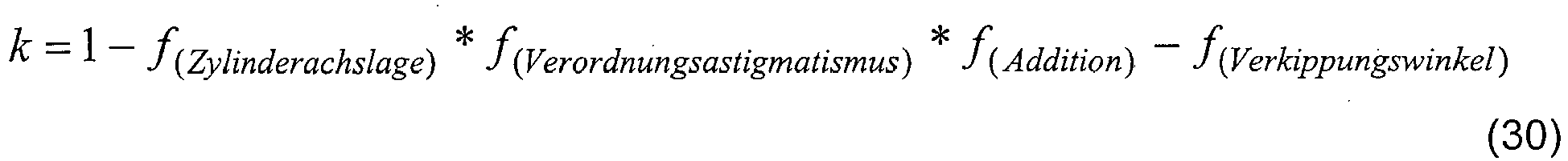

Ein Vorteil eines nach den Formeln (30) oder (31) berechneten Faktors k ist, dass der Faktor k automatisch einen Wert von 1 annimmt, wenn keine Transformation der Start-Sollastigmatismusverteilung stattfinden soll.An advantage of a factor k calculated according to the formulas (30) or (31) is that the factor k automatically assumes a value of 1 if no transformation of the starting target astigmatism distribution is to take place.
Vorzugsweise wird der Faktor k nur bei Verordnungszylinderachslagen von 0 bis 90° nach Tabo bei Angabe in Pluszylinderschreibweise bei rechten Gläsern, bei linken Gläsern bei Achslagen von 90 bis 180° angewendet. Bei Zylinderachslagen in diesen Bereichen treten die oben beschriebenen Nachteile verstärkt auf. Sind die Zylinderachslagen in den anderen Quadranten, so kann die Optimierung des Brillenglases nach dem konventionellen Verfahren (z.B. mit dem in
Nach der erfolgten Skalierung des temporalen Astigmatismus können die Sollastigmatismuswerte gegebenenfalls weiter skaliert oder transformiert werden. So kann z.B. die Progressionslänge analog zu f (Addition) von der Addition abhängen, wie in
Wie bereits oben ausgeführt, kann die Optimierung des Brillenglases anhand der transformierten Sollastigmatismusverteilung eine Minimierung einer Zielfunktion umfassen, in der die Werte der zuvor ermittelten transformierten Sollastigmatismusverteilung als Zielwerte eingehen. Vorzugsweise umfasst die Optimierung des Brillenglases anhand der transformierten Sollastigmatismusverteilung eine Minimierung einer Zielfunktion der Form: 
- Asti,Soll
neu den Sollastigmatismuswert der transformierten Sollastigmatismusverteilung AstSollneu an der i -ten Bewertungsstelle; - Asti den tatsächliche lokale Astigmatismus an der i -ten Bewertungsstelle; und
- gi,Ast die lokale Gewichtung des Sollastigmatismuswerts an der i -ten Bewertungsstelle
- Branch i, Soll
New the desired astigmatism value of the transformed target astigmatism distribution Ast SollNew at the i- th Assessment Body; - Branch i the actual local astigmatism at the i th assessment point; and
- g i, branch the local weighting of the target astigmatism value at the i th evaluation point
In der obigen Formel ist Asti,Soll
Ferner bevorzugt geht in die Zielfunktion ebenfalls der Refraktionsfehler/Brechwert ΔR ein, so dass das Berechnen bzw. Optimieren des Brillenglases eine Minimierung der Zielfunktion: 
- ΔRi,Soll
neu - den Sollwert des lokalen Refraktionsfehlers/Brechwerts an der i -ten Bewertungsstelle;
- ΔRi
- den tatsächlichen Wert des lokalen Refraktionsfehlers/Brechwerts an der i-ten Bewertungsstelle; und
- g i,ΔR
- die lokale Gewichtung der Refraktionsfehlers/Brechwerts an der i-ten Bewertungsstelle
- Δ R i, target
New - the set point of the local refractive error / refractive power at the i th evaluation point;
- ΔR i
- the actual value of the local refractive error / refractive power at the i th evaluation point; and
- g i , Δ R
- the local weighting of the refractive error / refractive power at the i th evaluation point
Die Verteilung des Sollbrechwerts oder des Sollrefraktionsfehlers kann ähnlich wie die Sollastigmatismusverteilung aus einer Start-Sollbrechwertverteilung oder einer Startsollrefraktionsfehlerverteilung ermittelt und durch Multiplikation mit einem Faktor abgeändert werden. Die Verteilung des Sollbrechwerts oder des Sollrefraktionsfehlers kann jedoch ebenfalls anhand der zuvor ermittelten, transformierten Sollastigmatismusverteilung ermittelt werden.The distribution of the target refractive power or the target refractive error can be determined similarly to the target astigmatism distribution from a starting target refractive power distribution or a starting target refractive error distribution and varied by multiplication by a factor. However, the distribution of the setpoint value or the desired refraction error can likewise be determined on the basis of the previously determined, transformed desired astigmatism distribution.
Vorzugsweise erfolgt die Optimierung des Brillenglases in Gebrauchsstellung des Brillenglases. Vorzugsweise werden bei der Optimierung des Brillenglases neben den individuellen Verordnungswerten (Sph, Zyl, Achse, Add, Prisma, Basis), Parameter der individuellen Lage bzw. Anordnung des Brillenglases vor dem Auge des Brillenträgers (z.B. Hornhautscheitelabstand (HSA), Fassungsscheibenwinkel (FSW), Vorneigung bzw. pantoskopischer Winkel) und/oder physiologische Parameter des Brillenträgers (z.B. Pupillendistanz) berücksichtigt. Alternativ können durchschnittliche Parameter der Lage bzw. Anordnung des Brillenglases vor dem Auge des Brillenträgers und/oder durchschnittliche physiologische Parameter des Brillenträgers berücksichtigt werden. Das progressive Brillenglas kann "online" nach Bestelleingang als Unikat optimiert und berechnet werden.The optimization of the spectacle lens preferably takes place in the position of use of the spectacle lens. In the optimization of the spectacle lens, in addition to the individual prescription values (Sph, Cyl, Axis, Add, Prism, Basis), parameters of the individual position or arrangement of the spectacle lens in front of the eye wearer's eye (eg corneal vertex distance (HSA), lens angle (FSW) , Preadjustment or pantoscopic angle) and / or physiological parameters of the wearer of the spectacle (eg pupillary distance). Alternatively, average parameters of the position or position of the spectacle lens in front of the eye wearer's eye and / or average physiological parameters of the spectacle wearer can be taken into account. The progressive spectacle lens can be optimized and calculated "online" after ordering as a unique item.
Vorzugsweise umfasst das Verfahren ferner die Schritte:
- Erfassen der Verordnungswerte des Brillenglases; und
- Erfassen der vorzugsweise individuellen Parameter des Brillenglases und/oder der Anordnung des Brillenglases vor den Augen des Brillenträgers.
- Detecting the prescription values of the spectacle lens; and
- Detecting the preferably individual parameters of the spectacle lens and / or the arrangement of the spectacle lens in front of the eyes of the spectacle wearer.
Mit der oben beschriebenen Vorgehensweise ist es möglich, bei einem bestehenden Gleitsichtglasdesign (Startdesign, Basisdesign) die für die Optimierung nach Zielfunktionen notwendige Sollastigmatismusverteilung für spezielle Wirkungen derart zu manipulieren, dass die Zielvorgabe leichter erreicht werden kann. Somit können die negativen Auswirkungen auf die optimierten Flächen- bzw. Gebrauchsstellungseigenschaften von nicht vorteilhaften Sollwertvorgaben deutlich reduziert werden. Dies verbessert auch direkt die Gebrauchsstellungseigenschaften.With the procedure described above, it is possible for an existing progressive lens design (start design, basic design) to manipulate the target astigmatism distribution for special effects necessary for the optimization according to target functions such that the target can be achieved more easily. Consequently For example, the negative effects on the optimized area or use position properties of non-advantageous setpoint specifications can be significantly reduced. This also directly improves the usage position properties.
Die oben beschriebene Verfahren sowie die entsprechende Vorrichtungen eignen sich sowohl für das Erzeugen von Designs bzw. Designvarianten für konventionelle oder wirkungsoptimierte progressive Brillengläser, als auch für das Erzeugen von Designs bzw. Designvarianten für individuell optimierte progressive Brillengläser.The methods described above and the corresponding devices are suitable both for the generation of designs or design variants for conventional or effect-optimized progressive spectacle lenses, as well as for the generation of designs or design variants for individually optimized progressive spectacle lenses.
Wie bereits oben ausgeführt, kann die Optimierung des Brillenglases eine Minimierung einer Zielfunktion umfassen, in der Sollwerte für den Sollastigmatismus und/oder für den Brechwertfehler (vgl. Gleichungen (18) und (18) oder Gleichungen (32) und (33)) eingehen. Die in die Zielfunktion eingehenden Werte können die gemäß dem oben beschriebenen Verfahren ermittelten Werte einer asymmetrischen Sollastigmatismusverteilung (AstSoll
Vorzugsweise erfolgt die Optimierung des Brillenglases in Gebrauchsstellung des Brillenglases. Vorzugsweise werden bei der Optimierung des Brillenglases neben den individuellen Verordnungswerten (Sph, Zyl, Achse, Add, Prisma, Basis), Parameter der individuellen Lage bzw. Anordnung des Brillenglases vor dem Auge des Brillenträgers (z.B. Hornhautscheitelabstand (HSA), Fassungsscheibenwinkel (FSW), Vorneigung bzw. pantoskopischer Winkel), physiologische Parameter des Brillenträgers (z.B. Pupillendistanz) berücksichtigt. Alternativ können durchschnittliche Parameter der Lage bzw. Anordnung des Brillenglases vor dem Auge des Brillenträgers und/oder durchschnittliche physiologische Parameter des Brillenträgers berücksichtigt werden. Das progressive Brillenglas kann online nach Bestelleingang als Unikat optimiert und berechnet werden.The optimization of the spectacle lens preferably takes place in the position of use of the spectacle lens. In the optimization of the spectacle lens, in addition to the individual prescription values (Sph, Cyl, Axis, Add, Prism, Basis), parameters of the individual position or arrangement of the spectacle lens in front of the eye wearer's eye (eg corneal vertex distance (HSA), lens angle (FSW) , Preadjustment or pantoscopic angle), physiological parameters of the spectacle wearer (eg pupillary distance) are taken into account. Alternatively, average parameters of the position or position of the spectacle lens in front of the eye wearer's eye and / or average physiological parameters of the spectacle wearer can be taken into account. The progressive spectacle lens can be optimized and calculated online after ordering as a unique.
Vorzugsweise umfasst das Verfahren ferner die Schritte:
- Erfassen der Verordnungswerte des Brillenglases; und
- Erfassen der vorzugsweise individuellen Parameter des Brillenglases und/oder der Anordnung des Brillenglases vor den Augen des Brillenträgers.
- Detecting the prescription values of the spectacle lens; and
- Detecting the preferably individual parameters of the spectacle lens and / or the arrangement of the spectacle lens in front of the eyes of the spectacle wearer.
Erfindungsgemäß werden ferner ein Computerprogrammerzeugnis, d.h. ein in der Patentanspruchskategorie einer Vorrichtung beanspruchtes Computerprogramm, sowie ein Speichermedium mit darauf gespeichertem Computerprogramm bereitgestellt, wobei das Computerprogramm ausgelegt ist, wenn geladen und ausgeführt auf einem Computer, ein bevorzugtes Verfahren zum Optimieren eines progressiven Brillenglases gemäß dem ersten Aspekt der Erfindung durchzuführen.According to the invention, a computer program product, i. a computer program claimed in the claim category of a device, and a storage medium with computer program stored thereon, the computer program being designed, when loaded and executed on a computer, to perform a preferred method for optimizing a progressive spectacle lens according to the first aspect of the invention.
Ferner wird gemäß einem weiteren Aspekt eine Vorrichtung zum Optimieren eines progressiven Brillenglases vorgeschlagen, umfassend Optimierungsmittel, welche ausgelegt sind, ein Berechnen bzw. Optimieren des Brillenglases nach einem bevorzugten Beispiels des Verfahrens zum Optimieren eines progressiven Brillenglases gemäß dem ersten Aspekt der Erfindung durchzuführen.Furthermore, according to a further aspect, a device for optimizing a progressive spectacle lens is proposed, comprising optimization means which are designed to perform an optimization of the spectacle lens according to a preferred example of the method for optimizing a progressive spectacle lens according to the first aspect of the invention.
Die Vorrichtung zum Optimieren eines progressiven Brillenglases kann:
- Objektabstandsfunktion-Vorgabemittel, welche ausgelegt sind, eine Start-Objektabstandsfunktion A 1G (y) vorzugeben oder festzulegen;
- Objektentfernungserfassungsmittel, welche ausgelegt sind, Objektentfernungsdaten zu erfassen, wobei die Objektentfernungsdaten eine Objektentfernung in zumindest einem vorgegebenen Punkt auf der Hauptblicklinie umfassen;
- Objektabstandsfunktionänderungsmittel zum Abändern bzw. Transformieren der Start-Objektabstandsfunktion in Abhängigkeit von den erfassten Objektentfernungsdaten; und
- Brillenglas-Optimierungsmittel zum Optimieren des progressiven Brillenglases, wobei bei der Optimierung des Brillenglases die transformierte Objektabstandsfunktion berücksichtigt wird,
- Object distance function specifying means configured to specify or set a start distance function A 1 G ( y );
- Object distance detection means adapted to detect object removal data, the object removal data including an object distance in at least one predetermined point on the main view line;
- Object distance function changing means for modifying the start-distance function in accordance with the detected object distance data; and
- Spectacle lens optimizing means for optimizing the progressive spectacle lens, wherein the transformed object distance function is taken into account in the optimization of the spectacle lens,
Die Objektabstandsfunktion gibt den reziproken Objektabstand bzw. die reziproke Objektentfernung entlang der Hauptblicklinie als Funktion der vertikalen Koordinate y an.The object distance function indicates the reciprocal object distance or the reciprocal object distance along the main line of sight as a function of the vertical coordinate y .
Das Abändern oder Transformieren der Start-Objektabstandsfunktion A 1G (y) umfasst ein Überlagern A 1(y)=A 1G (y)+A 1Korr (y) der Start-Objektabstandsfunktion A 1G (y) mit einer Korrekturfunktion A 1Korr (y). Die Korrekturfunktion weist zumindest einen variablen Parameter auf, welcher derart in Abhängigkeit von den erfassten Objektentfernungsdaten bestimmt wird, dass der Wert der abgeänderten Start-Objektabstandsfunktion in zumindest einem vorgegebenen Punkt gleich dem reziproken Wert der erfassten Sollobjektentfernung für diesen Punkt ist.Modifying or transforming the starting distance function A 1 G ( y ) comprises superimposing A 1 ( y ) = A 1 G ( y ) + A 1 Korr ( y ) of the starting distance function A 1 G ( y ) with a correction function A 1 corr ( y ). The correction function has at least one variable parameter, which is determined in dependence on the acquired object distance data such that the value of the modified start distance function in at least one predetermined point is equal to the reciprocal value of the detected solar object distance for that point.
Die Objektabstandsfunktion-Vorgabemittel können Speichermittel umfassen, in welchen die Start-Objektabstandsfunktion oder die Parameter der Start-Objektabstandsfunktion, anhand deren die Start-Objektabstandsfunktion rekonstruiert werden, kann dauerhaft oder temporär gespeichert werden. Die Objektentfernungserfassungsmittel können zumindest eine interaktive grafische Benutzerschnittstelle (GUI) umfassen, welche es einem Benutzer ermöglicht, Daten bezüglich der gewünschten Objektentfernungen in zumindest einem vorgegebenen Punkt anzugeben und gegebenenfalls zu verändern.The object distance function presetting means may comprise memory means in which the start distance function or the parameters of the start distance function, by means of which the start distance function is reconstructed, can be stored permanently or temporarily. The object distance detection means may comprise at least one interactive graphical user interface (GUI) which allows a user to specify and, if necessary, modify data regarding the desired object distances in at least one predetermined point.
Die Objektabstandsfunktionänderungsmittel und die Brillenglas-Optimierungsmittel können mittels entsprechend konfigurierten bzw. programmierten herkömmlichen Computern, spezialisierter Hardware und/oder Computernetzen bzw. Computersystemen implementiert werden. Der gleiche Computer bzw. das gleiche Computersystem, welcher/welches die Berechnung einer transformierten Objektabstandsfunktion (und gegebenenfalls einer transformierten Sollastigmatismusverteilung) durchführt, kann ebenfalls die Optimierung des Brillenglases nach der transformierten Objektabstandsfunktion durchführen. Es ist jedoch selbstverständlich möglich, dass die Berechnung der transformierten Objektabstandsfunktion und die Berechnung des Brillenglases nach der transformierten Objektabstandsfunktion in separaten Recheneinheiten, beispielsweise in separaten Computern oder Computersystemen erfolgen. Die Objektabstandsfunktionänderungsmittel und die Brillenglas-Optimierungsmittel können mittels geeigneter Schnittstellen miteinander in Signalverbindung stehen.The object distance function changing means and the spectacle lens optimizing means may be implemented by means of appropriately configured conventional computers, specialized hardware, and / or computer systems. The same computer or computer system which performs the calculation of a transformed object distance function (and possibly a transformed target astigmatism distribution) may also perform the optimization of the spectacle lens after the transformed object distance function. However, it is of course possible that the calculation of the transformed Object distance function and the calculation of the lens according to the transformed object distance function in separate computing units, for example, in separate computers or computer systems done. The object distance function changing means and the spectacle lens optimizing means may be in signal communication with each other by means of suitable interfaces.
Die Objektabstandsfunktionänderungsmittel können ebenfalls mittels geeigneter Schnittstellen in einer Signalverbindung mit dem Objektabstandsfunktion-Vorgabemittel stehen und insbesondere die in den Speichermitteln gespeicherten Daten auslesen und/oder modifizieren.The object distance function changing means can also be in a signal connection with the object distance function specifying means by means of suitable interfaces, and in particular can read out and / or modify the data stored in the storage means.
Ferner können die Objektabstandsfunktionänderungsmittel und/oder die Brillenglas-Optimierungsmittel vorzugsweise jeweils interaktive grafische Benutzerschnittstellen (GUI) umfassen, welche es einem Benutzer ermöglichen, die Berechnung der transformierten Objektabstandsfunktion und die Optimierung des progressiven Brillenglases zu visualisieren und gegebenenfalls durch Veränderung eines Parameters oder mehrerer Parameter zu steuern.Furthermore, the object distance function changing means and / or the spectacle lens optimizing means may each preferably comprise interactive graphical user interfaces (GUI) which enable a user to visualize the calculation of the transformed object distance function and the progressive spectacle lens optimization and, if necessary, by changing one or more parameters Taxes.
Zusätzlich kann die Vorrichtung zum Optimieren eines progressiven Brillenglases
- Speichermittel zum Speichern einer Start-Sollastigmatismusverteilung AstSoll
start für das progressive Brillenglas; - Sollastigmatismusverteilung-Berechnungsmittel, welche ausgelegt sind, eine transformierte Sollastigmatismusverteilung AstSoll
neu aus der Start-Sollastigmatismusverteilung zu ermitteln; und - Brillenglas-Optimierungsmittel, welche ausgelegt sind, ein progressives Brillenglases anhand der transformierten Sollastigmatismusverteilung zu optimieren.
- Storage means for storing a start-target astigmatism distribution Ast Soll
begin for the progressive spectacle lens; - Target astigmatism distribution calculating means which are adapted to a transformed target astigmatism distribution Ast Soll
New from the start-target astigmatism distribution; and - Spectacle lens optimizing means which are designed to optimize a progressive spectacle lens based on the transformed target astigmatism distribution.
Die Sollastigmatismusverteilung-Berechnungsmittel sind ausgelegt
- ein Multiplizieren des Werts des maximalen temporalen Sollastigmatismus max_AstSoll_temporalstart der Start-Sollastigmatismusverteilung AstSoll
start mit einem Faktor k:
- wodurch sich ein abgeänderter maximaler temporaler Astigmatismus max_AstSoll_temporalneu ergibt, wobei der Faktor k eine Funktion zumindest eines Verordnungswerts und/oder zumindest eines Parameters es Brillenglases oder dessen Anordnung vor den Augen des Brillenträgers ist; und
- ein Transformieren der Start-Sollastigmatismusverteilung AstSoll
start auf Basis des abgeänderten maximalen temporalen Astigmatismus max_AstSoll_temporalneu
- multiplying the value of the maximum temporal target astigmatism max_Ast target _temporal start the start target astigmatism distribution branch target
begin with a factor k : - whereby a modified maximum temporal astigmatism max _Ast Soll _temporal new results, wherein the factor k is a function of at least one prescription value and / or at least one parameter of spectacle lens or its arrangement in front of the eyes of the wearer; and
- transforming the start-target astigmatism distribution Ast Soll
begin on the basis of the modified maximum temporal astigmatism max _Ast should _temporal new
Die Start-Sollastigmatismusverteilung AstSoll
Die Sollastigmatismusverteilung-Berechnungsmittel und/oder die Brillenglas-Optimierungsmittel können mittels geeigneter Schnittstellen in einer Signalverbindung mit dem Speicher stehen und insbesondere die in dem Speicher gespeicherten Daten auslesen und/oder modifizieren. Ferner können die Sollastigmatismusverteilung-Berechnungsmittel und/oder die Brillenglas-Optimierungsmittel vorzugsweise jeweils interaktive grafische Benutzerschnittstellen (GUI) umfassen, welche es einem Benutzer ermöglichen, die Berechnung der transformierte Sollastigmatismusverteilung AstSoll
Gemäß einem weiteren Aspekt wird ein Verfahren zum Herstellen eines progressiven Brillenglases vorgeschlagen, umfassend:
- Optimieren des Brillenglases nach einem bevorzugten Beispiel des Verfahrens zum Optimieren eines progressiven Brillenglases gemäß dem ersten Aspekt der Erfindung,
- Bereitstellen von Flächendaten des berechneten bzw. optimierten Brillenglases; und
- Fertigen des Brillenglases gemäß den bereitgestellten Flächendaten des Brillenglases.
- Optimizing the spectacle lens according to a preferred example of the method for optimizing a progressive spectacle lens according to the first aspect of the invention,
- Providing area data of the calculated or optimized spectacle lens; and
- Finishing the spectacle lens according to the provided surface data of the spectacle lens.
Die Fertigung bzw. Bearbeitung des Brillenglases kann mittels CNC- Maschinen, mittels eines Gießverfahrens, einer Kombination der beiden Verfahren oder nach einem anderen geeigneten Verfahren erfolgen.The production or processing of the spectacle lens can take place by means of CNC machines, by means of a casting method, a combination of the two methods or by another suitable method.
Ebenfalls wird eine Vorrichtung zum Herstellen eines progressiven Brillenglases bereitgestellt, umfassend:
- Optimierungsmittel, welche ausgelegt sind, ein Berechnen bzw. Optimieren des Brillenglases nach einem bevorzugten Beispiel des Verfahrens zum Optimieren eines progressiven Brillenglases durchzuführen; und
- Bearbeitungsmittel zum Fertigbearbeiten des Brillenglases.
- Optimizing means configured to perform optimizing the spectacle lens according to a preferred example of the method for optimizing a progressive spectacle lens; and
- Processing means for finishing the spectacle lens.
Die Optimierungsmittel können die oben beschriebene Vorrichtung zum Optimieren eines progressiven Brillenglases sein.The optimizing means may be the above-described apparatus for optimizing a progressive spectacle lens.
Wie bereits oben ausgeführt können die Bearbeitungsmittel z.B. CNC gesteuerte Maschinen zur Direktbearbeitung eines Blanks nach den ermittelten Optimierungsvorgaben umfassen. Das fertigbearbeitete Brillenglas kann eine einfache sphärische oder rotationssymmetrisch asphärische Fläche und eine progressive Fläche aufweisen, wobei die progressive Fläche unter Berücksichtigung einer individuellen Objektanstandsfunktion und/oder einer (asymmetrischen) Sollastigmatismusverteilung sowie gegebenenfalls individueller Parameter des Brillenträgers optimiert wird. Vorzugsweise ist die sphärische oder rotationssymmetrisch asphärische Fläche die Vorderfläche (d.h. die objektseitige Fläche) des Brillenglases. Selbstverständlich ist es jedoch möglich, die nach dem berechneten Design optimierte Fläche als Vorderfläche des Brillenglases anzuordnen. Ebenfalls ist es möglich, dass beide Flächen des Brillenglases progressive Flächen sind. Des Weiteren ist es möglich, beide Flächen des Brillenglases zu optimieren.As already stated above, the processing means may include, for example, CNC-controlled machines for direct processing of a blanks according to the determined optimization specifications. The finished spectacle lens can be a simple spherical or rotationally symmetric aspherical surface and a have progressive surface, wherein the progressive surface is optimized taking into account an individual Objektanstandsfunktion and / or a (asymmetric) Sollastigmatismusverteilung and optionally individual parameters of the wearer. Preferably, the spherical or rotationally symmetric aspherical surface is the front surface (ie the object-side surface) of the spectacle lens. Of course, however, it is possible to arrange the surface optimized according to the calculated design as the front surface of the spectacle lens. It is also possible that both surfaces of the lens are progressive surfaces. Furthermore, it is possible to optimize both surfaces of the spectacle lens.
Die Vorrichtung zum Herstellen eines progressiven Brillenglases kann ferner Erfassungsmittel zum
- Erfassen der Verordnungswerte des Brillenglases; und
- Erfassen der (individuellen) Parameter des Brillenglases und/oder der Anordnung des Brillenglases vor den Augen des Brillenträgers
- Detecting the prescription values of the spectacle lens; and
- Detecting the (individual) parameters of the spectacle lens and / or the arrangement of the spectacle lens in front of the eyes of the spectacle wearer
Alternativ oder zusätzlich kann die Vorrichtung zum Herstellen eines progressiven Brillenglases ferner Erfassungsmittel zum Erfassen von Objektentfernungsdaten umfassen. Die Erfassungsmittel können insbesondere grafische Benutzerschnittstellen umfassen.Alternatively or additionally, the apparatus for producing a progressive spectacle lens may further comprise detection means for detecting object removal data. The detection means may in particular comprise graphical user interfaces.
Ferner wird ein progressives Brillenglas, welches nach einem bevorzugten Herstellungsverfahren hergestellt ist, vorgeschlagen, sowie eine Verwendung des nach einem bevorzugten Herstellungsverfahren hergestellten progressiven Brillenglases in einer vorgegebenen durchschnittlichen oder individuellen Gebrauchsstellung des Brillenglases vor den Augen eines bestimmten Brillenträgers zur Korrektur einer Fehlsichtigkeit des Brillenträgers.Further, a progressive spectacle lens, which is produced according to a preferred manufacturing method, proposed, as well as a use of the produced according to a preferred manufacturing process progressive spectacle lens in a predetermined average or individual use position of the spectacle lens in front of the eyes of a particular wearer for correcting a refractive error of the wearer.
Mit der vorgeschlagenen Vorgehensweise zur Abänderung der Objektabstandsfunktion gemäß einem der bevorzugten Beispiele ist es möglich, eine vorgegebene Start-Objektabstandsfunktion, welche z.B. einem Standard-Objektabstandmodell entspricht, schnell und mit einem vergleichsweise geringen Rechenaufwand an einem, von dem Standard-Objektabstandsmodell abweichenden Modell für die Objektentfernungen (Objektabstände) anzupassen. Es ist ferner möglich, die Charakteristika der Start-Objektabstandsfunktion gezielt zu ändern, und so Objektabstandsfunktion für unterschiedliche Brillenglasdesigns zu erzeugen.With the proposed procedure for modifying the object distance function according to one of the preferred examples, it is possible to use a predetermined start-distance function, which, for example, a Standard object distance model corresponds to adapt quickly and with a comparatively small amount of computation to a model for the object distances (object distances) that differs from the standard object distance model. It is also possible to selectively change the characteristics of the start-to-object distance function, and thus to create object distance function for different spectacle lens designs.
Weiteren Aufgaben, Merkmale und Vorteile der vorliegenden Erfindung gehen aus der nachfolgenden, detaillierten Beschreibung beispielhafter und bevorzugter Ausführungsformen der vorliegenden Erfindung mit Bezug auf die Zeichnungen hervor, in welchen zeigt:
- Fig. 1
- Start-Sollastigmatismusverteilung für eine
Addition von - Fig. 2
- Sollastigmatismusverteilung für eine
Addition von - Fig. 3
- die in
Fig. 2 gezeigte skalierte Sollastigmatismusverteilung, welche zusätzlich in Abhängigkeit von der Addition skaliert ist; - Fig.4
- die in Abhängigkeit von der Addition skalierte Start-Sollastigmatismusverteilung;
- Fig. 5
- einen Abschnitt einer graphischen Benutzerschnittstelle zum Festlegen des Vorfaktors v;
- Fig. 6A
- ein Beispiel einer Start-Sollastigmatismusverteilung;
- Fig. 6B
- ein Beispiel einer abgeänderten/transformierten Sollastigmatismusverteilung, welche aus der in
Fig. 6A gezeigten Start-Sollastigmatismusverteilung berechnet wurde; - Fig. 7A
- den Flächenbrechwert der progressiven Fläche eines progressiven Brillenglases, welches nach der in
Fig. 6A gezeigten Start-Sollastigmatismusverteilung optimiert worden ist; - Fig. 7B
- den Flächenbrechwert der progressiven Fläche eines progressiven Brillenglases, welches nach der in
Fig. 6B gezeigten transformierten Sollastigmatismusverteilung optimiert worden ist; - Fig. 8A
- den Gradient des Flächenbrechwerts der progressiven Fläche des progressiven Brillenglases, welches nach der in
Fig. 6A gezeigten Start-Sollastigmatismusverteilung optimiert worden ist; - Fig. 8B
- den Gradient des Flächenbrechwerts der progressiven Fläche des progressiven Brillenglases, welches nach der in
Fig. 6B gezeigten transformierten Sollastigmatismusverteilung optimiert worden ist; - Fig. 9A
- den Flächenastigmatismus der progressiven Fläche des progressiven Brillenglases, welches nach der in
Fig. 6A gezeigten Start-Sollastigmatismusverteilung optimiert worden ist; - Fig. 9B
- den Flächenastigmatismus der progressiven Fläche des progressiven Brillenglases, welches nach der in
Fig. 6B gezeigten transformierten Sollastigmatismusverteilung optimiert worden ist; - Fig. 10A
- den Gradient des Flächenastigmatismus der progressiven Fläche des progressiven Brillenglases, welches nach der in
Fig. 6A gezeigten Start-Sollastigmatismusverteilung optimiert worden ist; - Fig. 10B
- den Gradient des Flächenastigmatismus der progressiven Fläche des progressiven Brillenglases, welches nach der in
Fig. 6B gezeigten transformierten Sollastigmatismusverteilung optimiert worden ist; - Fig. 11A
- den Astigmatismus in Gebrauchstellung des progressiven Brillenglases, welches nach der in
Fig. 6A gezeigten Start-Sollastigmatismusverteilung optimiert worden ist; - Fig. 11B
- den Astigmatismus in Gebrauchstellung des progressiven Brillenglases, welches nach der in
Fig. 6B gezeigten transformierten Sollastigmatismusverteilung optimiert worden ist; - Fig. 12A
- den mittleren Brechwert in Gebrauchstellung des progressiven Brillenglases, welches nach der in
Fig. 6A gezeigten Start-Sollastigmatismusverteilung optimiert worden ist; - Fig. 12B
- den mittleren Brechwert in Gebrauchstellung des progressiven Brillenglases welches nach der in
Fig. 6B gezeigten transformierten Sollastigmatismusverteilung optimiert worden ist; - Fig.13A,B
- die Abbildung von Objekten in unterschiedlichen Objektentfernungen durch ein Brillenglas;
- Fig.14A,B
- den reziproken Objektanstand (in dpt) entlang der Hauptblicklinie gemäß einem Beispiel;
- Fig. 15A - 15H
- ein Beispiel einer Anpassung einer Start-Objektabstandsfunktion an ein geändertes Objektabstandsmodell, wobei
Fig. 15A eine weitere beispielhafte Start-Objektanstandsfunktion;
Fig. 15B die Steigung der Start-Objektanstandsfunktion;
Fig. 15C eine beispielhafte Gauss'sche Funktion;
Fig. 15D die Steigung der Gauss'schen Funktion;
Fig. 15E die durch eine Überlagerung der Start-Objektabstandsfunktion mit der Gauss'schen Funktion erhaltene Objektabstandsfunktion;
Fig. 15F die Steigung der Objektabstandsfunktion;
Fig. 15G die durch eine lineare Anpassung abgeänderte Objektabstandsfunktion; und
Fig. 15H die Steigung der durch eine lineare Anpassung abgeänderten Objektabstandsfunktion ist; - Fig. 16A -16C
- ein Beispiel einer graphischen Benutzerschnittstelle zur Visualisierung und Änderung der Objektabstandsfunktion, wobei
Fig. 16A einen Abschnitt zur Visualisierung einer Start-Objektabstandsfunktion;
Fig. 16B einen Abschnitt zur Visualisierung und Änderung der Parameter einer Korrekturfunktion;
Fig. 16C einen Abschnitt zur Visualisierung der abgeänderten Start-Objektabstandsfunktion ist; - Fig. 17A-17C
- ein weiteres Beispiel einer Anpassung einer Start-Objektabstandsfunktion an ein geänderten Objektabstandsmodell, wobei
Fig. 17A eine weitere beispielhafte Start-Objektanstandsfunktion;
Fig. 17B die Steigung der Start-Objektanstandsfunktion;
Fig. 17C die durch eine lineare Anpassung erhaltene neue Objektabstandsfunktion;
Fig. 17D die Steigung der neuen Objektabstandsfunktion ist; - Fig. 18
- eine beispielhafte graphische Benutzerschnittstelle zur Visualisierung und Änderung der Objektabstandsfunktion;
- Fig.19
- eine weitere beispielhafte graphische Benutzerschnittstelle zur Visualisierung und Änderung der Objektabstandsfunktion.
- Fig. 1
- Start-target astigmatism distribution for an addition of 2.5 dpt;
- Fig. 2
- Target astigmatism distribution for addition of 2.5 D with scaling of temporal astigmatism;
- Fig. 3
- in the
Fig. 2 shown scaled target astigmatism distribution, which is additionally scaled in dependence on the addition; - Figure 4
- the scaled start-target astigmatism distribution as a function of the addition;
- Fig. 5
- a portion of a graphical user interface for setting the pre-factor v;
- Fig. 6A
- an example of a start-target astigmatism distribution;
- Fig. 6B
- an example of a modified / transformed Sollastigmatismusverteilung, which from the in
Fig. 6A calculated start-target astigmatism distribution has been calculated; - Fig. 7A
- the surface refractive index of the progressive surface of a progressive spectacle lens, which after the in
Fig. 6A shown start-target astigmatism distribution has been optimized; - Fig. 7B
- the surface refractive index of the progressive surface of a progressive spectacle lens, which after the in
Fig. 6B shown transformed Sollastigmatismusverteilung has been optimized; - Fig. 8A
- the gradient of the surface power of the progressive surface of the progressive spectacle lens, which after the in
Fig. 6A shown Start-target astigmatism distribution has been optimized; - Fig. 8B
- the gradient of the surface power of the progressive surface of the progressive spectacle lens, which after the in
Fig. 6B shown transformed Sollastigmatismusverteilung has been optimized; - Fig. 9A
- the surface astigmatism of the progressive surface of the progressive spectacle lens, which after the in
Fig. 6A shown start-target astigmatism distribution has been optimized; - Fig. 9B
- the surface astigmatism of the progressive surface of the progressive spectacle lens, which after the in
Fig. 6B shown transformed Sollastigmatismusverteilung has been optimized; - Fig. 10A
- the gradient of the surface astigmatism of the progressive surface of the progressive spectacle lens, which after the in
Fig. 6A shown start-target astigmatism distribution has been optimized; - Fig. 10B
- the gradient of the surface astigmatism of the progressive surface of the progressive spectacle lens, which after the in
Fig. 6B shown transformed Sollastigmatismusverteilung has been optimized; - Fig. 11A
- the astigmatism in the use position of the progressive spectacle lens, which after the in
Fig. 6A shown start-target astigmatism distribution has been optimized; - Fig. 11B
- the astigmatism in the use position of the progressive spectacle lens, which after the in
Fig. 6B shown transformed Sollastigmatismusverteilung has been optimized; - Fig. 12A
- the average power in the use position of the progressive spectacle lens, which after the in
Fig. 6A shown start-target astigmatism distribution has been optimized; - Fig. 12B
- the average power in the use position of the progressive spectacle lens which after the in
Fig. 6B shown transformed Sollastigmatismusverteilung has been optimized; - 13A, B
- the imaging of objects in different object distances through a spectacle lens;
- 14A, B
- the reciprocal object condition (in dpt) along the main line of vision according to an example;
- Figs. 15A-15H
- an example of adaptation of a start-distance function to a modified object distance model, wherein
Fig. 15A shows another exemplary startup object function;
Fig. 15B shows the slope of the start object feature function;
Fig. 15C is an exemplary Gaussian function;
Fig. 15D shows the slope of the Gaussian function;
15E shows the object distance function obtained by superposing the start distance function with the Gaussian function;
Fig. 15F shows the slope of the object distance function;
FIG. 15G shows the object distance function modified by a linear adaptation; FIG. and
Fig. 15H is the slope of the object distance function modified by a linear fit; - Figs. 16A-16C
- an example of a graphical user interface for visualizing and changing the object distance function, wherein
Fig. 16A is a portion for visualizing a start-distance feature;
16B shows a section for visualizing and changing the parameters of a correction function;
Fig. 16C is a section for visualizing the modified start distance function; - Figs. 17A-17C
- Another example of an adaptation of a start-distance function to a modified object distance model, wherein
FIG. 17A is another exemplary startup object function; FIG.
Fig. 17B shows the slope of the start object feature function;
Fig. 17C shows the new object distance function obtained by a linear fit;
Fig. 17D is the slope of the new object distance function; - Fig. 18
- an exemplary graphical user interface for visualizing and changing the object distance function;
- Figure 19
- another exemplary graphical user interface for visualizing and changing the object distance function.
Auf der Abszisse der
In einem Beispiel wird in Abhängigkeit von den Verordnungsdaten des Brillenglases (insbesondere des Verordnungsastigmatismus, der verordneten Achse des Verordnungsastigmatismus und der verordneten Addition) und des Verkippungswinkels des Brillenglases ein Faktor k = 0,58 ermittelt (vgl. Gleichungen (7) bis (13)). Der Faktor k = 0,58 wird mit dem maximalen temporalen Astigmatismus der Start-Sollastigmatismusverteilung multipliziert. Anschließend wird eine Interpolation der Sollastigmatismuswerte zwischen der 0,5 dpt Basis-Sollisoastigmatismuslinie und der Peripherie des Brillenglases unter Berücksichtigung des mit dem Faktor k multiplizierten maximalen temporalen Astigmatismus durchgeführt. Die Interpolation erfolgt nach dem in
In diesem Beispiel hat die Multiplikation des maximalen temporalen Astigmatismus mit dem Faktor k keinen Einfluss auf die 0,5 dpt Basis-Sollisoastigmatismuslinie. Die Sollastigmatismuswerte zwischen der Hauptlinie und der 0,5 dpt Basis-Sollisoastigmatismuslinie bleiben somit unverändert. Zwischen der temporalen 0,5 dpt Basis-Sollisoastigmatismuslinie und der Spitze des temporalen Astigmatismushügels (d.h. die Position des maximalen Sollastigmatismus) wird jedoch eine Interpolation anhand des skalierten maximalen temporalen Astigmatismus (in diesem Fall 2,6 * 0,58 = 1,508 dpt) durchgeführt.
Wie in der
- Sphäre (Sph) = -8 dpt;
- Zylinder (Cyl) = 6 dpt;
- Achse 45°;
Addition 0,75 dpt.
- Sphere (Sph) = -8 dpt;
- Cylinder (Cyl) = 6 dpt .;
- Axis 45 °;
- Addition 0.75 Dpt.
Der Verkippungswinkel, welcher bei flachen Basiskurven näherungsweise dem Fassungsscheibenwinkel entspricht, beträgt 5°.The tilt angle, which corresponds approximately to the frame disc angle for flat base curves, is 5 °.
Nach den oben beschriebenen Formeln (7) bis (14) ergibt sich ein Faktor k mit einem Wert von 0,58.According to formulas (7) to (14) described above, a factor k of 0.58 results.
Fig. X-A (X = 6, 7, ...12) beziehen sich auf ein Vergleichsbeispiel mit einer symmetrischen Sollastigmatismusverteilung ("Start-Sollastigmatismusverteilung"). Fig. X-B (X = 6, 7, ..., 12) beziehen sich auf ein Beispiel ("Manipulierte Sollvorgaben) mit einer nicht symmetrischen
Sollastigmatismusverteilung. FIG. XA (X = 6, 7,... 12) refer to a comparative example with a symmetrical target astigmatism distribution ("starting target astigmatism distribution"). Fig. XB (X = 6, 7, ..., 12) refer to an example ("Manipulated Setpoints) with a non-symmetric
Astigmatism distribution.
Die in
Bei einem Vergleich der
Die progressive Fläche des Brillenglases, welches gemäß den in
Ferner ist bei einem Vergleich der
Ebenfalls sind die Gebrauchsstellungseigenschaften (Astigmatismus und Brechwert in Gebrauchsstellung) des gemäß den manipulierten Sollastigmatismusvorgaben optimierten Brillenglases deutlich gradientenärmer, wobei sich die zentralen Sehbereiche nicht wesentlich in ihrer Größe und Nutzbarkeit unterscheiden. In dem konkreten Beispiel ändern sich die Gradienten von 0,45 dpt/mm zu 0,05 dpt/mm. Bei dem mittleren Brechwert in Gebrauchsstellung wird eine Reduktion von 0,55 dpt/mm (vgl.
- a1= 1/A 1
- die Objektentfernung (den Objektabstand);
- e den
- Hornhautscheitelabstand (HSA);
- b'
- den Augendrehpunktabstand;
- sZ'
- den Abstand Hornhautscheitel - Augendrehpunkt;
- s'BG
- die Bildentfernung;
- Z'
- den Augendrehpunkt;
- R
- die Fernpunktkugel; und
- SK
- die Scheitelpunktkugel.
- a1 = 1 / A 1
- the object distance (the object distance);
- e the
- Corneal vertex distance (HSA);
- b '
- the eye pivot distance;
- s Z '
- the distance corneal vertex - eye pivot;
- s' BG
- the image removal;
- Z '
- the eye pivot point;
- R
- the far-end sphere; and
- SK
- the vertex ball.
Die Berechnung bzw. Optimierung des Brillenglases 10 erfolgt komplett in der Gebrauchsstellung des Brillenglases 12, d.h. unter Berücksichtung der vorgegebenen Anordnung des Brillenglases vor den Augen 12 des Brillenträgers (definiert durch den Hornhautscheitelabstand, Vorneigung, etc.) und eines vorgegebenen Objektabstandmodells. Das Objektabstandsmodell kann die Vorgabe einer Objektfläche 14 umfassen, welche verschiedene Objektabstände oder Objektbereiche für foveales Sehen festlegt. Die Objektfläche 14 wird vorzugsweise durch die Vorgabe der reziproken Objektentfernung (des reziproken Objektabstands) A 1(x,y) entlang der objektseitigen Hauptstrahlen definiert. Der Verlauf der reziproken Objektentfernung A 1(x=x0 , y)=A 1(u=0, y) entlang der Hauptblicklinie (d.h. bei x=x 0 bzw. u=0) stellt die Objektabstandsfunktion dar. Die Objektabstandsfunktion A 1(x=x 0 , y)=A 1(u=0,y) bestimmt die Breite der Sehbereiche in der Umgebung der Hauptblicklinie (Satz von Minkwitz). Ein Punkt auf der Objektfläche wird vom Brillenglas auf die Fernpunktkugel abgebildet, wie in
Gemäß einem ersten Beispiel wird die Objektabstandsfunktion A 1(y) als Summe zweier Doppelasymptotenfunktionen dargestellt.
Die Parameter der Start-Objektabstandsfunktion (welche durch eine Doppelasymptotenfunktion beschrieben wird) sind aG = 2,606 dpt, bG = -2,588 dpt, c=-0,46/mm, d=2,2 mm und m = 0,75.The parameters of the start-distance function (which is described by a double asymptotic function) are a G = 2.606 D, b G = -2.588 D, c = -0.46 / mm, d = 2.2 mm and m = 0.75.
In diesem Fall ist der Fernbezugspunkt DF (Designpunkt Ferne) bei y = +8 mm (yDF =8 mm) und der Nahbezugspunkt DN (Designpunkt Nähe) bei y = -12 mm (yDN = -12 mm). Die Objektentfernung im Fernbezugspunkt ist unendlich und folglich A 1Ferne = A 1G (yDF ) = 0,00 dpt. Die Objektentfernung im Nahbezugspunkt ist - 40 cm und folglich A 1Nähe = A 1G (yDN ) = -2,50 dpt. In this case, the distance reference point DF (design point distance) at y = +8 mm ( y DF = 8 mm) and the near reference point DN (design point proximity) at y = -12 mm ( y DN = -12 mm). The object distance in the far reference point is infinite and hence A 1 distance = A 1 G ( y DF ) = 0.00 dpt. The object distance in the near reference point is - 40 cm and, consequently, near A 1 = A 1 G (y DN) = - 2.50 dpt.
Die Objektentfernungen im Fern- und Nahbezugspunkte für einen bestimmten Brillenträger oder für andere Designs und Anwendungen können jedoch von dem obigen Standardmodell abweichen. Beispielsweise kann im Fernbezugspunkt DF eine Objektentfernung von -400 cm und im Nahbezugspunkt eine Objektentfernung von -50 cm berücksichtigt werden. Für diesen Fall sind die abgeänderten Sollvorgaben für die Objektentfernungen in den Fern- und Nahbezugspunkten A 1Ferne = A 1G (yDF ) = -0,25 dpt und A 1Nähe = A 1G (yDN ) = -2,00 dpt.However, the distance and near reference object distances for a particular wearer of glasses or for other designs and applications may differ from the standard model above. For example, an object distance of -400 cm in the distance reference point DF and an object distance of -50 cm in the near reference point can be taken into account. For this case, the modified target specifications for the object distances at the far and near reference points A 1 are distance = A 1 G ( y DF ) = -0.25 D and A 1 proximity = A 1 G ( y DN ) = -2.00 diopter.
Durch eine Überlagerung der Start-Objektabstandsfunktion A 1G (y) mit einer Korrekturfunktion A 1Korr (y) mit den gleichen Koeffizienten c, d und m, wie die der Start-Objektabstandsfunktion und mit den Koeffizienten bkorr = 0,526 und akorr = -0,782, ergibt sich der in
![]()
![]()
Die in
- A 1(y=10) = -0,50 dpt und
- A 1(y = -14) = -2,50 dpt
- A 1 ( y = 10) = -0.50 D and
- A 1 ( y = -14) = -2.50 dpt
Die abgeänderte bzw. angepasste Objektabstandsfunktion wird nach der Formel A 1neu (y)=c+(1+m)A 1(y) erhalten, wobei c = 0,836 und m = 0,335 gilt.The modified object distance function is obtained according to the formula A 1 new ( y ) = c + (1+ m ) A 1 ( y ), where c = 0.836 and m = 0.335.
![]()
![]()

-
Fig. 17A zeigt den Verlauf der Funktion A 1 G(y) entlang der Hauptlinie in dpt; -
Fig. 17B zeigt die erste Ableitung
-
Fig. 17A shows the course of the function A 1 G (y) along the main line in dpt; -
Fig. 17B shows the first derivative
Die in
-
Fig. 17C den Verlauf der neuen Objektabstandsfunktion A 1(y) entlang der Hauptlinie auf der Vorderfläche des Brillenglases; und -
Fig. 17D die Ableitung
-
Fig. 17C the course of the new object distance function A 1 ( y ) along the main line on the front surface of the spectacle lens; and -
Fig. 17D the derivative
- 1010
- Brillenglaslens
- 1212
- Auge des BrillenträgersEye of the spectacle wearer
- 1414
- ObjektflächeProperty area
- ee
- Hornhautscheitelabstand (HSA)Corneal Vertex Distance (HSA)
- b'b '
- AugendrehpunktabstandOcular pivot point distance
- sZ'sZ '
- Abstand Hornhautscheitel - AugendrehpunktDistance corneal vertex - eye pivot
- s'BGs'BG
- Bildentfernungimage Distance
- Z'Z '
- AugendrehpunktRotation of the eye
- RR
- FernpunktkugelFar point sphere
- SKSK
- ScheitelpunktkugelApex ball
Claims (11)
- Computer-implemented method for optimising a progressive spectacle lens, comprising the steps of:specifying an initial object distance function A 1G (y),acquiring object distance data, wherein the object distance data comprise an object distance at at least one specified point in the main line of sight;modifying the initial object distance function on the basis of the acquired object distance data;optimising the progressive spectacle lens, wherein the modified object distance function is taken into account when optimising the spectacle lens, whereinthe modification of the initial object distance function A 1G (y) comprises superposition A 1(y) = A 1G (y) + A 1Korr (y) of the initial object distance function A 1G (y) on a correction function A 1Korr (y), wherein the correction function comprises at least one variable parameter that is determined on the basis of the acquired object distance data such that the value of the modified initial object distance function is equal, at at least one specified point, to the reciprocal value of the acquired target object distance for this point, and whereinthe object distance function is defined as the reciprocal object distance along the main line of sight and y is the vertical coordinate,wherein the correction function is a doubly asymptotic function
 having the parameters akorr , bkorr, ckorr, dkorr, mkorr , wherein the parameters bkorr and akorr of the correction function are determined on the basis of the acquired object distance data; orwherein the correction function is a linear function of the initial object distance function AKorr (y) = c + mA 1G (y) having the parameters c and m.
 - Method according to claim 1, wherein the object distance data comprise at least one target object distance A 1Feme at a specified far reference point in the main line of sight and a target object distance A1Nähe at a specified near reference point in the main line of sight.
- Method according to either claim 1 or claim 2, wherein the initial object distance function is a doubly asymptotic function

- Method according to claim 3, wherein the correction function is a doubly asymptotic function, and wherein c = ckorr , d = dkorr, m = mkorr is true for the parameters of the correction function.
- Method according to claim 2, wherein the correction function is a linear function of the initial object distance function, wherein the following is true for the parameters c and m:


 A 1Ferne denotes the reciprocal value of the target object distance in the far reference point;A 1Nähe denotes the reciprocal value of the target object distance in the near reference point;yF denotes the vertical coordinate of the far reference point; andyN denotes the vertical coordinate of the near reference point.
 - Method according to any of the preceding claims, further comprising superposing the initial object distance function A 1G (y) on a function that is a Gaussian bell curve

- Computer program product that is designed, when loaded and executed on a computer, to carry out a method for optimising a progressive spectacle lens according to any of claims 1 to 8.
- Storage medium comprising a computer program stored thereon, wherein the computer program is designed, when loaded and executed on a computer, to carry out a method for optimising a progressive spectacle lens according to any of claims 1 to 6.
- Apparatus for optimising a progressive spectacle lens, comprising optimisation means that are designed to optimise the spectacle lens according to the method according to any of claims 1 to 6.
- Method for producing a progressive spectacle lens, comprising:- optimising the spectacle lens according to the method according to any of claims 1 to 6,- providing surface data of the computed and/or optimised spectacle lens, and- manufacturing the spectacle lens according to the spectacle lens surface data provided.
- Apparatus for producing a progressive spectacle lens, comprising:- optimisation means that are designed to optimise the spectacle lens according to the method according to any of claims 1 to 6; and- machining means for final machining of the spectacle lens.
Applications Claiming Priority (2)
| Application Number | Priority Date | Filing Date | Title |
|---|---|---|---|
| DE201010049168 DE102010049168A1 (en) | 2010-10-21 | 2010-10-21 | Regulation and individualization-dependent modification of the temporal peripheral target astigmatism and adaptation of the object distance function to changed object distances for proximity and / or distance |
| EP20110776091 EP2630544B1 (en) | 2010-10-21 | 2011-10-13 | Prescription-dependent and individualization-dependent modification of the temporal peripheral nominal astigmatism and adaptation of the object distance function to changed object distances for near and/or far vision |
Related Parent Applications (2)
| Application Number | Title | Priority Date | Filing Date |
|---|---|---|---|
| EP20110776091 Division EP2630544B1 (en) | 2010-10-21 | 2011-10-13 | Prescription-dependent and individualization-dependent modification of the temporal peripheral nominal astigmatism and adaptation of the object distance function to changed object distances for near and/or far vision |
| EP20110776091 Division-Into EP2630544B1 (en) | 2010-10-21 | 2011-10-13 | Prescription-dependent and individualization-dependent modification of the temporal peripheral nominal astigmatism and adaptation of the object distance function to changed object distances for near and/or far vision |
Publications (2)
| Publication Number | Publication Date |
|---|---|
| EP2767862A1 EP2767862A1 (en) | 2014-08-20 |
| EP2767862B1 true EP2767862B1 (en) | 2017-09-27 |
Family
ID=44883163
Family Applications (2)
| Application Number | Title | Priority Date | Filing Date |
|---|---|---|---|
| EP20110776091 Active EP2630544B1 (en) | 2010-10-21 | 2011-10-13 | Prescription-dependent and individualization-dependent modification of the temporal peripheral nominal astigmatism and adaptation of the object distance function to changed object distances for near and/or far vision |
| EP14001194.1A Active EP2767862B1 (en) | 2010-10-21 | 2011-10-13 | Prescription-dependent and individualization-dependent adaptation of the object distance function to changed object distances for near and/or far vision |
Family Applications Before (1)
| Application Number | Title | Priority Date | Filing Date |
|---|---|---|---|
| EP20110776091 Active EP2630544B1 (en) | 2010-10-21 | 2011-10-13 | Prescription-dependent and individualization-dependent modification of the temporal peripheral nominal astigmatism and adaptation of the object distance function to changed object distances for near and/or far vision |
Country Status (5)
| Country | Link |
|---|---|
| US (2) | US9176331B2 (en) |
| EP (2) | EP2630544B1 (en) |
| DE (1) | DE102010049168A1 (en) |
| ES (1) | ES2649148T3 (en) |
| WO (1) | WO2012052133A1 (en) |
Families Citing this family (8)
| Publication number | Priority date | Publication date | Assignee | Title |
|---|---|---|---|---|
| EP2270577A1 (en) * | 2009-06-30 | 2011-01-05 | Essilor International (Compagnie Générale D'Optique) | Method of and apparatus for generating a surface of an optical lens |
| US10261341B2 (en) * | 2012-11-14 | 2019-04-16 | Essilor International | Method for determining the feasibility of an ophthalmic lens |
| EP3074810B1 (en) * | 2013-11-25 | 2017-11-15 | Essilor International (Compagnie Générale d'Optique) | A method for providing to a wearer a customized progressive spectacle ophthalmic lens |
| DE102015205721B4 (en) * | 2015-03-30 | 2017-01-19 | Rodenstock Gmbh | Method for creating a design of a prescription surface of a multifocal lens and multifocal lens with such a prescription surface |
| JP6496019B2 (en) | 2015-05-26 | 2019-04-03 | ホヤ レンズ タイランド リミテッドHOYA Lens Thailand Ltd | Progressive power lens design method and design apparatus |
| US10401649B2 (en) | 2015-05-26 | 2019-09-03 | Hoya Lens Thailand Ltd. | Method of designing progressive refractive power lens, and lens set |
| US10274750B2 (en) | 2016-07-21 | 2019-04-30 | National Taiwan University Of Science And Technology | Progressive multifocal contact lens and producing method thereof |
| ES2687223A1 (en) * | 2017-04-21 | 2018-10-24 | Horizons Optical S.L.U. | Procedure for optimizing a progressive ophthalmic lens and its manufacturing procedure. (Machine-translation by Google Translate, not legally binding) |
Family Cites Families (11)
| Publication number | Priority date | Publication date | Assignee | Title |
|---|---|---|---|---|
| EP1277079B1 (en) | 2000-04-25 | 2006-03-29 | Rodenstock GmbH | Method for calculating a progressive spectacle lens and method for producing a spectacle lens of this type |
| ATE391305T1 (en) * | 2000-04-25 | 2008-04-15 | Rodenstock Gmbh | PROGRESSIVE GOGGLES LENS |
| DE10310354B4 (en) * | 2003-03-10 | 2006-07-27 | Rodenstock Gmbh | Method for optimizing a progressive spectacle lens |
| DE102004059448A1 (en) | 2004-11-19 | 2006-06-01 | Rodenstock Gmbh | Method and apparatus for manufacturing a spectacle lens; System and computer program product for manufacturing a spectacle lens |
| FR2894688B1 (en) | 2005-12-13 | 2008-02-15 | Essilor Int | METHOD FOR DETERMINING A SET OF PROGRESSIVE MULTIFOCAL OPHTHALMIC LENSES |
| DE112008000049A5 (en) * | 2007-01-25 | 2009-09-10 | Rodenstock Gmbh | Flexible progressive lens optimizer |
| DE102008015189A1 (en) | 2008-03-20 | 2009-10-01 | Rodenstock Gmbh | Rescaling the target astigmatism for other additions |
| DE102009005206A1 (en) | 2009-01-20 | 2010-07-22 | Rodenstock Gmbh | Variable progressive lens design |
| DE102009005214A1 (en) | 2009-01-20 | 2010-07-22 | Rodenstock Gmbh | Automatic progressive lens design modification |
| DE112010000759A5 (en) | 2009-01-23 | 2012-08-02 | Rodenstock Gmbh | Design control by means of a design polygon |
| CN103443693B (en) * | 2011-03-07 | 2015-04-01 | 依视路国际集团(光学总公司) | Method for determining progressive ophthalmic lens |
-
2010
- 2010-10-21 DE DE201010049168 patent/DE102010049168A1/en not_active Ceased
-
2011
- 2011-10-13 EP EP20110776091 patent/EP2630544B1/en active Active
- 2011-10-13 WO PCT/EP2011/005144 patent/WO2012052133A1/en active Application Filing
- 2011-10-13 EP EP14001194.1A patent/EP2767862B1/en active Active
- 2011-10-13 ES ES14001194.1T patent/ES2649148T3/en active Active
- 2011-10-13 US US13/880,922 patent/US9176331B2/en active Active
-
2015
- 2015-01-09 US US14/593,050 patent/US9638935B2/en active Active
Non-Patent Citations (1)
| Title |
|---|
| None * |
Also Published As
| Publication number | Publication date |
|---|---|
| US9176331B2 (en) | 2015-11-03 |
| DE102010049168A1 (en) | 2012-04-26 |
| EP2767862A1 (en) | 2014-08-20 |
| ES2649148T3 (en) | 2018-01-10 |
| US20150116657A1 (en) | 2015-04-30 |
| WO2012052133A1 (en) | 2012-04-26 |
| EP2630544B1 (en) | 2014-10-01 |
| US20140049747A1 (en) | 2014-02-20 |
| EP2630544A1 (en) | 2013-08-28 |
| US9638935B2 (en) | 2017-05-02 |
Similar Documents
| Publication | Publication Date | Title |
|---|---|---|
| EP2767862B1 (en) | Prescription-dependent and individualization-dependent adaptation of the object distance function to changed object distances for near and/or far vision | |
| DE69938027T9 (en) | Toric ophthalmic lenses | |
| EP1606668B1 (en) | Method for calculating an individual progressive lens | |
| EP2115525B1 (en) | Flexible varifocal lens optimizer | |
| EP2389609B1 (en) | Automatic modification of a progressive lens design | |
| EP2564262B1 (en) | Method for calculating a spectacle lens using viewing angle-dependent prescription data | |
| EP2263114B1 (en) | Rescaling of the target astigmatism for other additions | |
| EP2389610B1 (en) | Variable progressive lens design | |
| DE102006030204A1 (en) | Pair of spectacle lenses in anisometropia | |
| EP3824343B1 (en) | Varifocal spectacle lens with a spatially varying refractive index | |
| DE102015205721B4 (en) | Method for creating a design of a prescription surface of a multifocal lens and multifocal lens with such a prescription surface | |
| DE102005023126B4 (en) | Series of spectacle lenses, manufacturing process | |
| EP3814828B1 (en) | Computer-implemented method, data processing system for producing a target design and computer program, storage medium having instructions for producing a target design, method for providing a spectacle lens, storage medium having a numerical representation of a spectacle lens and method for manufacturing a spectacle lens | |
| EP4193217A1 (en) | Improved calculation of ophthalmological lenses | |
| DE102017118219B4 (en) | Computer-implemented method for creating a target design for optimizing a free-form surface of a spectacle lens, computer program, storage medium, computer and device | |
| DE102017118721B4 (en) | Computer-implemented method and device for transforming a plurality of first points of a first lens surface into a plurality of second points of a second lens surface, computer-implemented method and device for determining a target lens with an optimized lens surface and computer program | |
| WO2018137962A1 (en) | Method for taking into consideration different long-distance and short-distance prismatic corrections | |
| EP3789815A1 (en) | Computer-implemented method for adapting spectacle lens to spectacle frame |
Legal Events
| Date | Code | Title | Description |
|---|---|---|---|
| PUAI | Public reference made under article 153(3) epc to a published international application that has entered the european phase |
Free format text: ORIGINAL CODE: 0009012 |
|
| 17P | Request for examination filed |
Effective date: 20140331 |
|
| AC | Divisional application: reference to earlier application |
Ref document number: 2630544 Country of ref document: EP Kind code of ref document: P |
|
| AK | Designated contracting states |
Kind code of ref document: A1 Designated state(s): AL AT BE BG CH CY CZ DE DK EE ES FI FR GB GR HR HU IE IS IT LI LT LU LV MC MK MT NL NO PL PT RO RS SE SI SK SM TR |
|
| 111Z | Information provided on other rights and legal means of execution |
Free format text: AL AT BE BG CH CY CZ DE DK EE ES FI FR GB GR HR HU IE IS IT LT LU LV MC MK MT NL NO PL PT RO RS SE SI SK SM TR Effective date: 20141010 |
|
| R17P | Request for examination filed (corrected) |
Effective date: 20150122 |
|
| RBV | Designated contracting states (corrected) |
Designated state(s): AL AT BE BG CH CY CZ DE DK EE ES FI FR GB GR HR HU IE IS IT LI LT LU LV MC MK MT NL NO PL PT RO RS SE SI SK SM TR |
|
| 17Q | First examination report despatched |
Effective date: 20161205 |
|
| GRAJ | Information related to disapproval of communication of intention to grant by the applicant or resumption of examination proceedings by the epo deleted |
Free format text: ORIGINAL CODE: EPIDOSDIGR1 |
|
| GRAP | Despatch of communication of intention to grant a patent |
Free format text: ORIGINAL CODE: EPIDOSNIGR1 |
|
| INTG | Intention to grant announced |
Effective date: 20170424 |
|
| GRAS | Grant fee paid |
Free format text: ORIGINAL CODE: EPIDOSNIGR3 |
|
| GRAA | (expected) grant |
Free format text: ORIGINAL CODE: 0009210 |
|
| RIN1 | Information on inventor provided before grant (corrected) |
Inventor name: ESSER, GREGOR Inventor name: ZIMMERMANN, MARTIN Inventor name: WELK, ANDREA Inventor name: BECKEN, WOLFGANG Inventor name: KASTER, ROBERT Inventor name: UTTENWEILER, DIETMAR Inventor name: ALTHEIMER, HELMUT |
|
| AC | Divisional application: reference to earlier application |
Ref document number: 2630544 Country of ref document: EP Kind code of ref document: P |
|
| AK | Designated contracting states |
Kind code of ref document: B1 Designated state(s): AL AT BE BG CH CY CZ DE DK EE ES FI FR GB GR HR HU IE IS IT LI LT LU LV MC MK MT NL NO PL PT RO RS SE SI SK SM TR |
|
| REG | Reference to a national code |
Ref country code: GB Ref legal event code: FG4D Free format text: NOT ENGLISH Ref country code: FR Ref legal event code: PLFP Year of fee payment: 7 |
|
| REG | Reference to a national code |
Ref country code: CH Ref legal event code: EP |
|
| REG | Reference to a national code |
Ref country code: AT Ref legal event code: REF Ref document number: 932481 Country of ref document: AT Kind code of ref document: T Effective date: 20171015 |
|
| REG | Reference to a national code |
Ref country code: IE Ref legal event code: FG4D Free format text: LANGUAGE OF EP DOCUMENT: GERMAN |
|
| REG | Reference to a national code |
Ref country code: DE Ref legal event code: R096 Ref document number: 502011013068 Country of ref document: DE |
|
| REG | Reference to a national code |
Ref country code: ES Ref legal event code: FG2A Ref document number: 2649148 Country of ref document: ES Kind code of ref document: T3 Effective date: 20180110 |
|
| PG25 | Lapsed in a contracting state [announced via postgrant information from national office to epo] |
Ref country code: SE Free format text: LAPSE BECAUSE OF FAILURE TO SUBMIT A TRANSLATION OF THE DESCRIPTION OR TO PAY THE FEE WITHIN THE PRESCRIBED TIME-LIMIT Effective date: 20170927 Ref country code: FI Free format text: LAPSE BECAUSE OF FAILURE TO SUBMIT A TRANSLATION OF THE DESCRIPTION OR TO PAY THE FEE WITHIN THE PRESCRIBED TIME-LIMIT Effective date: 20170927 Ref country code: LT Free format text: LAPSE BECAUSE OF FAILURE TO SUBMIT A TRANSLATION OF THE DESCRIPTION OR TO PAY THE FEE WITHIN THE PRESCRIBED TIME-LIMIT Effective date: 20170927 Ref country code: HR Free format text: LAPSE BECAUSE OF FAILURE TO SUBMIT A TRANSLATION OF THE DESCRIPTION OR TO PAY THE FEE WITHIN THE PRESCRIBED TIME-LIMIT Effective date: 20170927 Ref country code: NO Free format text: LAPSE BECAUSE OF FAILURE TO SUBMIT A TRANSLATION OF THE DESCRIPTION OR TO PAY THE FEE WITHIN THE PRESCRIBED TIME-LIMIT Effective date: 20171227 |
|
| REG | Reference to a national code |
Ref country code: NL Ref legal event code: MP Effective date: 20170927 |
|
| REG | Reference to a national code |
Ref country code: LT Ref legal event code: MG4D |
|
| PG25 | Lapsed in a contracting state [announced via postgrant information from national office to epo] |
Ref country code: GR Free format text: LAPSE BECAUSE OF FAILURE TO SUBMIT A TRANSLATION OF THE DESCRIPTION OR TO PAY THE FEE WITHIN THE PRESCRIBED TIME-LIMIT Effective date: 20171228 Ref country code: RS Free format text: LAPSE BECAUSE OF FAILURE TO SUBMIT A TRANSLATION OF THE DESCRIPTION OR TO PAY THE FEE WITHIN THE PRESCRIBED TIME-LIMIT Effective date: 20170927 Ref country code: LV Free format text: LAPSE BECAUSE OF FAILURE TO SUBMIT A TRANSLATION OF THE DESCRIPTION OR TO PAY THE FEE WITHIN THE PRESCRIBED TIME-LIMIT Effective date: 20170927 Ref country code: BG Free format text: LAPSE BECAUSE OF FAILURE TO SUBMIT A TRANSLATION OF THE DESCRIPTION OR TO PAY THE FEE WITHIN THE PRESCRIBED TIME-LIMIT Effective date: 20171227 |
|
| PG25 | Lapsed in a contracting state [announced via postgrant information from national office to epo] |
Ref country code: NL Free format text: LAPSE BECAUSE OF FAILURE TO SUBMIT A TRANSLATION OF THE DESCRIPTION OR TO PAY THE FEE WITHIN THE PRESCRIBED TIME-LIMIT Effective date: 20170927 |
|
| PG25 | Lapsed in a contracting state [announced via postgrant information from national office to epo] |
Ref country code: RO Free format text: LAPSE BECAUSE OF FAILURE TO SUBMIT A TRANSLATION OF THE DESCRIPTION OR TO PAY THE FEE WITHIN THE PRESCRIBED TIME-LIMIT Effective date: 20170927 Ref country code: CZ Free format text: LAPSE BECAUSE OF FAILURE TO SUBMIT A TRANSLATION OF THE DESCRIPTION OR TO PAY THE FEE WITHIN THE PRESCRIBED TIME-LIMIT Effective date: 20170927 |
|
| PG25 | Lapsed in a contracting state [announced via postgrant information from national office to epo] |
Ref country code: EE Free format text: LAPSE BECAUSE OF FAILURE TO SUBMIT A TRANSLATION OF THE DESCRIPTION OR TO PAY THE FEE WITHIN THE PRESCRIBED TIME-LIMIT Effective date: 20170927 Ref country code: SK Free format text: LAPSE BECAUSE OF FAILURE TO SUBMIT A TRANSLATION OF THE DESCRIPTION OR TO PAY THE FEE WITHIN THE PRESCRIBED TIME-LIMIT Effective date: 20170927 Ref country code: SM Free format text: LAPSE BECAUSE OF FAILURE TO SUBMIT A TRANSLATION OF THE DESCRIPTION OR TO PAY THE FEE WITHIN THE PRESCRIBED TIME-LIMIT Effective date: 20170927 Ref country code: IS Free format text: LAPSE BECAUSE OF FAILURE TO SUBMIT A TRANSLATION OF THE DESCRIPTION OR TO PAY THE FEE WITHIN THE PRESCRIBED TIME-LIMIT Effective date: 20180127 |
|
| REG | Reference to a national code |
Ref country code: CH Ref legal event code: PL |
|
| REG | Reference to a national code |
Ref country code: DE Ref legal event code: R097 Ref document number: 502011013068 Country of ref document: DE |
|
| PG25 | Lapsed in a contracting state [announced via postgrant information from national office to epo] |
Ref country code: MC Free format text: LAPSE BECAUSE OF FAILURE TO SUBMIT A TRANSLATION OF THE DESCRIPTION OR TO PAY THE FEE WITHIN THE PRESCRIBED TIME-LIMIT Effective date: 20170927 |
|
| REG | Reference to a national code |
Ref country code: IE Ref legal event code: MM4A |
|
| PG25 | Lapsed in a contracting state [announced via postgrant information from national office to epo] |
Ref country code: LI Free format text: LAPSE BECAUSE OF NON-PAYMENT OF DUE FEES Effective date: 20171031 Ref country code: DK Free format text: LAPSE BECAUSE OF FAILURE TO SUBMIT A TRANSLATION OF THE DESCRIPTION OR TO PAY THE FEE WITHIN THE PRESCRIBED TIME-LIMIT Effective date: 20170927 Ref country code: LU Free format text: LAPSE BECAUSE OF NON-PAYMENT OF DUE FEES Effective date: 20171013 Ref country code: CH Free format text: LAPSE BECAUSE OF NON-PAYMENT OF DUE FEES Effective date: 20171031 |
|
| PLBE | No opposition filed within time limit |
Free format text: ORIGINAL CODE: 0009261 |
|
| STAA | Information on the status of an ep patent application or granted ep patent |
Free format text: STATUS: NO OPPOSITION FILED WITHIN TIME LIMIT |
|
| REG | Reference to a national code |
Ref country code: BE Ref legal event code: MM Effective date: 20171031 |
|
| PG25 | Lapsed in a contracting state [announced via postgrant information from national office to epo] |
Ref country code: PL Free format text: LAPSE BECAUSE OF FAILURE TO SUBMIT A TRANSLATION OF THE DESCRIPTION OR TO PAY THE FEE WITHIN THE PRESCRIBED TIME-LIMIT Effective date: 20170927 Ref country code: BE Free format text: LAPSE BECAUSE OF NON-PAYMENT OF DUE FEES Effective date: 20171031 |
|
| 26N | No opposition filed |
Effective date: 20180628 |
|
| PG25 | Lapsed in a contracting state [announced via postgrant information from national office to epo] |
Ref country code: MT Free format text: LAPSE BECAUSE OF FAILURE TO SUBMIT A TRANSLATION OF THE DESCRIPTION OR TO PAY THE FEE WITHIN THE PRESCRIBED TIME-LIMIT Effective date: 20170927 |
|
| PG25 | Lapsed in a contracting state [announced via postgrant information from national office to epo] |
Ref country code: IE Free format text: LAPSE BECAUSE OF NON-PAYMENT OF DUE FEES Effective date: 20171013 |
|
| REG | Reference to a national code |
Ref country code: FR Ref legal event code: PLFP Year of fee payment: 8 |
|
| PG25 | Lapsed in a contracting state [announced via postgrant information from national office to epo] |
Ref country code: SI Free format text: LAPSE BECAUSE OF FAILURE TO SUBMIT A TRANSLATION OF THE DESCRIPTION OR TO PAY THE FEE WITHIN THE PRESCRIBED TIME-LIMIT Effective date: 20170927 |
|
| REG | Reference to a national code |
Ref country code: AT Ref legal event code: MM01 Ref document number: 932481 Country of ref document: AT Kind code of ref document: T Effective date: 20171013 |
|
| PG25 | Lapsed in a contracting state [announced via postgrant information from national office to epo] |
Ref country code: AT Free format text: LAPSE BECAUSE OF NON-PAYMENT OF DUE FEES Effective date: 20171013 |
|
| PG25 | Lapsed in a contracting state [announced via postgrant information from national office to epo] |
Ref country code: HU Free format text: LAPSE BECAUSE OF FAILURE TO SUBMIT A TRANSLATION OF THE DESCRIPTION OR TO PAY THE FEE WITHIN THE PRESCRIBED TIME-LIMIT; INVALID AB INITIO Effective date: 20111013 |
|
| PG25 | Lapsed in a contracting state [announced via postgrant information from national office to epo] |
Ref country code: CY Free format text: LAPSE BECAUSE OF NON-PAYMENT OF DUE FEES Effective date: 20170927 |
|
| PG25 | Lapsed in a contracting state [announced via postgrant information from national office to epo] |
Ref country code: MK Free format text: LAPSE BECAUSE OF FAILURE TO SUBMIT A TRANSLATION OF THE DESCRIPTION OR TO PAY THE FEE WITHIN THE PRESCRIBED TIME-LIMIT Effective date: 20170927 |
|
| PG25 | Lapsed in a contracting state [announced via postgrant information from national office to epo] |
Ref country code: TR Free format text: LAPSE BECAUSE OF FAILURE TO SUBMIT A TRANSLATION OF THE DESCRIPTION OR TO PAY THE FEE WITHIN THE PRESCRIBED TIME-LIMIT Effective date: 20170927 |
|
| PG25 | Lapsed in a contracting state [announced via postgrant information from national office to epo] |
Ref country code: PT Free format text: LAPSE BECAUSE OF FAILURE TO SUBMIT A TRANSLATION OF THE DESCRIPTION OR TO PAY THE FEE WITHIN THE PRESCRIBED TIME-LIMIT Effective date: 20170927 |
|
| PG25 | Lapsed in a contracting state [announced via postgrant information from national office to epo] |
Ref country code: AL Free format text: LAPSE BECAUSE OF FAILURE TO SUBMIT A TRANSLATION OF THE DESCRIPTION OR TO PAY THE FEE WITHIN THE PRESCRIBED TIME-LIMIT Effective date: 20170927 |
|
| PGFP | Annual fee paid to national office [announced via postgrant information from national office to epo] |
Ref country code: GB Payment date: 20231025 Year of fee payment: 13 |
|
| PGFP | Annual fee paid to national office [announced via postgrant information from national office to epo] |
Ref country code: ES Payment date: 20231117 Year of fee payment: 13 |
|
| PGFP | Annual fee paid to national office [announced via postgrant information from national office to epo] |
Ref country code: IT Payment date: 20231031 Year of fee payment: 13 Ref country code: FR Payment date: 20231023 Year of fee payment: 13 Ref country code: DE Payment date: 20231011 Year of fee payment: 13 |