EP2685291A2 - Method for exploiting a geological deposit from a deposit model matched by calculating an analytic law of the conditional distribution of uncertain parameters of the model - Google Patents
Method for exploiting a geological deposit from a deposit model matched by calculating an analytic law of the conditional distribution of uncertain parameters of the model Download PDFInfo
- Publication number
- EP2685291A2 EP2685291A2 EP13305753.9A EP13305753A EP2685291A2 EP 2685291 A2 EP2685291 A2 EP 2685291A2 EP 13305753 A EP13305753 A EP 13305753A EP 2685291 A2 EP2685291 A2 EP 2685291A2
- Authority
- EP
- European Patent Office
- Prior art keywords
- reservoir
- model
- models
- law
- parameters
- Prior art date
- Legal status (The legal status is an assumption and is not a legal conclusion. Google has not performed a legal analysis and makes no representation as to the accuracy of the status listed.)
- Granted
Links
- 238000000034 method Methods 0.000 title claims abstract description 79
- 238000009826 distribution Methods 0.000 title claims description 65
- 238000004590 computer program Methods 0.000 claims abstract description 3
- 230000006870 function Effects 0.000 claims description 94
- 238000010276 construction Methods 0.000 claims description 10
- 238000002474 experimental method Methods 0.000 claims description 5
- 230000035945 sensitivity Effects 0.000 claims description 4
- 238000004891 communication Methods 0.000 claims description 2
- 238000004088 simulation Methods 0.000 description 25
- 230000004044 response Effects 0.000 description 24
- 238000004519 manufacturing process Methods 0.000 description 22
- 230000008569 process Effects 0.000 description 15
- 239000012530 fluid Substances 0.000 description 11
- 239000007789 gas Substances 0.000 description 11
- 238000012360 testing method Methods 0.000 description 9
- 230000003068 static effect Effects 0.000 description 8
- 238000004364 calculation method Methods 0.000 description 7
- 230000035699 permeability Effects 0.000 description 7
- 230000006399 behavior Effects 0.000 description 5
- 229930195733 hydrocarbon Natural products 0.000 description 5
- 150000002430 hydrocarbons Chemical class 0.000 description 5
- 238000005259 measurement Methods 0.000 description 5
- 238000011084 recovery Methods 0.000 description 5
- 239000003208 petroleum Substances 0.000 description 4
- XLYOFNOQVPJJNP-UHFFFAOYSA-N water Substances O XLYOFNOQVPJJNP-UHFFFAOYSA-N 0.000 description 4
- 102100036109 Dual specificity protein kinase TTK Human genes 0.000 description 3
- 101000659223 Homo sapiens Dual specificity protein kinase TTK Proteins 0.000 description 3
- 101100024083 Saccharomyces cerevisiae (strain ATCC 204508 / S288c) MPH2 gene Proteins 0.000 description 3
- 238000013459 approach Methods 0.000 description 3
- 230000015572 biosynthetic process Effects 0.000 description 3
- 230000001143 conditioned effect Effects 0.000 description 3
- 238000005755 formation reaction Methods 0.000 description 3
- 238000012986 modification Methods 0.000 description 3
- 230000004048 modification Effects 0.000 description 3
- 238000005457 optimization Methods 0.000 description 3
- 238000003860 storage Methods 0.000 description 3
- 238000007792 addition Methods 0.000 description 2
- 238000012550 audit Methods 0.000 description 2
- 230000001419 dependent effect Effects 0.000 description 2
- 238000006073 displacement reaction Methods 0.000 description 2
- 238000005516 engineering process Methods 0.000 description 2
- 238000013401 experimental design Methods 0.000 description 2
- 230000006872 improvement Effects 0.000 description 2
- 230000010354 integration Effects 0.000 description 2
- 230000010355 oscillation Effects 0.000 description 2
- 238000010408 sweeping Methods 0.000 description 2
- 101100137549 Arabidopsis thaliana PRF5 gene Proteins 0.000 description 1
- 102100022361 CAAX prenyl protease 1 homolog Human genes 0.000 description 1
- 239000004215 Carbon black (E152) Substances 0.000 description 1
- 101000824531 Homo sapiens CAAX prenyl protease 1 homolog Proteins 0.000 description 1
- 101001003584 Homo sapiens Prelamin-A/C Proteins 0.000 description 1
- 101000577630 Homo sapiens Vitamin K-dependent protein S Proteins 0.000 description 1
- 208000035871 PIK3CA-related overgrowth syndrome Diseases 0.000 description 1
- 101150054426 PRO4 gene Proteins 0.000 description 1
- 241000135309 Processus Species 0.000 description 1
- 101100311302 Sordaria macrospora (strain ATCC MYA-333 / DSM 997 / K(L3346) / K-hell) pro11 gene Proteins 0.000 description 1
- 241001080024 Telles Species 0.000 description 1
- 238000004422 calculation algorithm Methods 0.000 description 1
- 238000012512 characterization method Methods 0.000 description 1
- 230000001427 coherent effect Effects 0.000 description 1
- 230000001955 cumulated effect Effects 0.000 description 1
- 238000005553 drilling Methods 0.000 description 1
- 238000011156 evaluation Methods 0.000 description 1
- 238000013213 extrapolation Methods 0.000 description 1
- 238000002347 injection Methods 0.000 description 1
- 239000007924 injection Substances 0.000 description 1
- 230000002452 interceptive effect Effects 0.000 description 1
- 239000007937 lozenge Substances 0.000 description 1
- 238000010606 normalization Methods 0.000 description 1
- 239000003921 oil Substances 0.000 description 1
- 229940052586 pro 12 Drugs 0.000 description 1
- 238000012545 processing Methods 0.000 description 1
- 230000000644 propagated effect Effects 0.000 description 1
- 239000000700 radioactive tracer Substances 0.000 description 1
- 230000009467 reduction Effects 0.000 description 1
- 230000000717 retained effect Effects 0.000 description 1
- 238000005070 sampling Methods 0.000 description 1
- 239000000243 solution Substances 0.000 description 1
Images


Classifications
-
- G01V20/00—
-
- G—PHYSICS
- G06—COMPUTING; CALCULATING OR COUNTING
- G06F—ELECTRIC DIGITAL DATA PROCESSING
- G06F30/00—Computer-aided design [CAD]
- G06F30/20—Design optimisation, verification or simulation
- G06F30/28—Design optimisation, verification or simulation using fluid dynamics, e.g. using Navier-Stokes equations or computational fluid dynamics [CFD]
-
- E—FIXED CONSTRUCTIONS
- E21—EARTH DRILLING; MINING
- E21B—EARTH DRILLING, e.g. DEEP DRILLING; OBTAINING OIL, GAS, WATER, SOLUBLE OR MELTABLE MATERIALS OR A SLURRY OF MINERALS FROM WELLS
- E21B41/00—Equipment or details not covered by groups E21B15/00 - E21B40/00
-
- E—FIXED CONSTRUCTIONS
- E21—EARTH DRILLING; MINING
- E21B—EARTH DRILLING, e.g. DEEP DRILLING; OBTAINING OIL, GAS, WATER, SOLUBLE OR MELTABLE MATERIALS OR A SLURRY OF MINERALS FROM WELLS
- E21B2200/00—Special features related to earth drilling for obtaining oil, gas or water
- E21B2200/20—Computer models or simulations, e.g. for reservoirs under production, drill bits
Definitions
- the present invention relates to the technical field of the petroleum industry, and more particularly to the operation of underground reservoirs, such as petroleum reservoirs or gas storage sites.
- a reservoir model is a model of the subsoil, representative of both its structure and its behavior. Generally, this type of model is represented on a computer, and one speaks then of numerical model.
- a reservoir model comprises a mesh or grid, generally three-dimensional, associated with one or more petrophysical property maps (porosity, permeability, saturation, etc.). The association consists of assigning values of these petrophysical properties to each grid cell.
- a representative reservoir model is done in stages. First, we build a reservoir model based on static data. Then this model is updated to best reproduce historical data via flow simulation while maintaining consistency with static data.
- History calibration consists of modifying the parameters of a reservoir model, such as permeabilities, porosities or well skins (representing the damage around the well), fault connections ..., to minimize the differences between the measured history data and the corresponding responses simulated from the reservoir model.
- Parameters may be related to geographic areas such as permeabilities or porosities around a well or several wells.
- the gap between the historical data and the simulated answers forms a functional, called objective function. The problem of history matching is solved by minimizing this functional.
- This approach therefore has two levels of approximation: the first concerns the convergence of the MCMC algorithm, of which it is very difficult to say whether it has converged towards the desired law; the second concerns the approximation of the objective function by the response surface.
- the object of the invention relates to a method of operating a geological reservoir according to an exploitation scheme defined from a reservoir model.
- the reservoir model is obtained by a probabilistic "history calibration" technique taking into account an analytical law of conditional distribution of uncertain parameters associated with a given response surface.
- this response surface does not approach the objective function itself but another function determined from the objective function. This makes it possible to obtain better approximations of the objective function and thus of the posterior law.
- the use of an analytical law makes it possible to reduce the calculation times, to consider a much faster processing of the results and to obtain a representative reservoir model by limiting the approximations.
- said values of G ( ⁇ i ) are interpolated by a kriging technique.
- step iv) at each iteration several new reservoir models are generated, from which M 1 models are selected that are added to said set, said set of reservoir models is constituted during the construction of the reservoir. initial set of a number M 0 of models.
- said M 0 models of said initial set are sampled by a Latin hypercube type experiment plane technique.
- said model M 1 added in said set are chosen using the approximation of said function G ( ⁇ ).
- At least a part of said model M 1 are the models for which the approximation of the function G ( ⁇ ) gives the maximum values.
- model M 1 may be the models for which the quality of the approximation of the function G ( ⁇ ) has the highest kriging variances among the said new models.
- a sensitivity study can be performed by calculating several objective functions, each objective function being calculated for a part of the parameters or for a limited time interval with respect to the information available.
- the invention also relates to a computer program product downloadable from a communication network and / or recorded on a computer readable medium and / or executable by a processor. It includes program code instructions for carrying out the method as described above, when said program is run on a computer.
- the method of the invention is intended for the exploitation of an underground reservoir, this operation may consist of the recovery of hydrocarbons but also the storage of gas, such as CO 2 in the reservoir.
- gas such as CO 2
- the uncertain parameters can be related to any part of the reservoir model. For example, they may be parameters to fill the reservoir model with petrophysical properties (permeability, porosity), parameters characterizing the wells (skins), the fluids in place or injected (saturation with residual oil after sweeping with the water or gas for example) or the tank structure (fault connections).
- a set of parameter values ⁇ ( ⁇ 1 ... ⁇ P ), which also corresponds to a point in the parameter space, therefore defines a reservoir model.
- a modification of each parameter therefore leads to a modification of the reservoir model.
- the uncertain parameter is related to the spatial distribution of a petrophysical property, it may be necessary to use a geostatistical simulation technique to generate the associated reservoir model.
- Geological formations are generally very heterogeneous environments.
- Reservoir modeling ie the construction of a reservoir model that respects static data, requires the use of so-called “probabilistic” construction processes because of the limited information available ( number of restricted wells, ).
- geological models constructed from these probabilistic processes are called “stochastic models”.
- the construction of a stochastic reservoir model must first depend on the environment of the geological repository, which allows to represent the major heterogeneities that control the flow of fluids.
- the integration of static data in this model involves linear operations and can be done from geostatistical techniques well known to specialists. For this, one can advantageously use a geostatistical simulator.
- a reservoir model which can be represented on a computer, comprises an N-dimensional grid (N> 0 and in general equal to two or three) each of whose meshes is assigned the value of a characteristic property of the zone studied. This may be, for example, the porosity or the permeability distributed in a reservoir. These values constitute maps. Thus a model includes a grid associated with at least one map. Other parameters characterizing for example wells or injected fluids are also involved in the definition of this model.
- an initial set of reservoir models is generated stochastically by means of the prior probability law p ( ⁇ ) of each uncertain parameter.
- a sample (X1) of M 0 values according to the prior distribution law p ( ⁇ i ) is generated, for example from a method experience plan of the Latin hypercube type.
- p ( ⁇ i ) a sample of M 0 values according to the prior distribution law p ( ⁇ i ) is generated, for example from a method experience plan of the Latin hypercube type.
- the purpose of the calibration process according to the invention is to construct a reservoir model that is as representative as possible.
- dynamic data has not been considered to build the initial reservoir model.
- DD dynamic data during the exploitation of the deposit
- It is production data, well tests, breakthrough time, 4D seismic ... whose particularity is to vary over time depending on the flow of fluid in the tank.
- These measurements are made using measuring tools such as flow meters or seismic sensors.
- ( y 1 ... y n ) the vector of the observed dynamic data and ( t 1 ... t n ) the corresponding acquisition times.
- the flows in the reservoir models to be evaluated are simulated, ie either the reservoir models of the set initial, ie the reservoir models generated during the previous iteration.
- the recovery of oil or the displacements of the fluids can be simulated in the tank.
- the inverse problem in reservoir engineering is to look for the value of uncertain parameters of the reservoir model that, applied to the flow simulator, provide a simulated response as close as possible to the measured dynamic data.
- the objective is to use the observed data to derive information on the vector of the uncertain parameters ⁇ .
- p ( ⁇ ) is the distribution law a priori
- p ( y 1 , ..., y n ) is the distribution law of the data
- ⁇ ) is the law conditional distribution of dynamic data knowing ⁇
- ( y 1 , ..., y n ) is the conditional posterior distribution law sought.
- the response surface used by the invention approaches not the objective function, but a function dependent on this objective function.
- the function G ( ⁇ ) is between 0 and 1, and therefore varies in a narrower range than the function F ( ⁇ ). Consequently, it is easier to construct a good approximation of the function G ( ⁇ ) than of the function F ( ⁇ ).
- the interpolation method used is a kriging technique or any other regression method belonging to the family of penalized empirical risk minimization in reproducing kernel Hilbert spaces (RKHS of the English Reproducting Kernel Hilbert Space).
- RKHS kernel Hilbert spaces
- G ⁇ ( ⁇ ) the function (or response surface) G ⁇ ( ⁇ ) in the form of a linear combination of known functions.
- y 1 , ..., y n ) associated with G ⁇ ( ⁇ ) then involves different integrals of these known functions, which are analytically computable.
- New reservoir models are generated, that is to say new sets of uncertain parameter values, as a function of the analytic law p ( ⁇
- p ⁇
- the reservoir models corresponding to each new set of values of the previously selected parameters are then generated. This may require the use of a geostatistical simulator to generate the petrophysical properties of the reservoir model.
- a criterion Q2 it is possible to define a criterion Q2 by removing groups of stitches rather than a single stitch.
- Other types of quality criteria may also be used.
- the quality criterion Q 2 is better if the strong values of G are well predicted. In our case, these strong values correspond to values of parameters for which the objective function is weak, that is to say to values where the adequacy with the historical data is good.
- a high Q 2 criterion means that the objective function is correctly approached for parameters corresponding to a good history setting.
- a reservoir model calibrated with the dynamic data amounts to associating with the uncertain parameters (or calibration of the model) the value corresponding to the lowest value of the objective function.
- a model of reservoir calibrated with the dynamic data and according to the probabilistic method described previously amounts to associating with the uncertain parameters (or calibration of the model) their posterior probability law.
- a standard objective function is used.
- F s ⁇ / s F ⁇ where s is a normalization constant.
- This involves constructing an approximation of BOY WUT s ⁇ exp - / s F ⁇ .
- the final posterior probability distribution of the objective function is sampled by an MCMC method, after evaluation of a model of F ( ⁇ ) by kriging.
- the specialists can determine several exploitation plans (SE) corresponding to different possible options for the exploitation of the underground reservoir: location of the wells producer and / or injector, target values for the flows per well and / or for the reservoir, the type of tools used, the fluids used and recovered ... For each of these schemes, it is necessary to determine their production forecasts after the calibration period.
- SE exploitation plans
- These probabilistic production forecasts are obtained by means of flow simulator software (preferably the same as that used previously) as well as by means of the calibrated reservoir model.
- SE possible exploitation schemes
- the reservoir is then exploited according to the chosen exploitation scheme (EX), for example by drilling new wells (producer or injector), by modifying the flows and / or the injected fluids.
- EX chosen exploitation scheme
- one may decide to set the value of one or more of the parameters and look at the impact on the uncertainty of the other parameters as well as on the objective function (s) chosen. In this case, it suffices to recalculate analytically the conditional distribution law of the parameters ⁇ j , j 1 ... N, j ⁇ i conditioned to the value chosen for ⁇ i .
- the applicant has carried out two series of experiments.
- the first series concerns the obtaining of posterior distributions.
- the second series illustrates the good correlation between the analytic law associated with the response surfaces and the exact conditional distribution law.
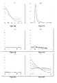
- the reservoir initially contains gas, oil and water. It is closed by faults on two sides, and by an aquifer on the other sides. Production is by depletion from six wells (PRO1 PRO4, PROS, PRO11, PRO12, PRO15) with an oil production rate of 150 m 3 / day imposed on each producing well for 10 years. During this production period, the accumulated oil (V) and the gas / oil ratio (R) are collected for each producing well, as well as the accumulated total oil in the reservoir. These values are known with a relative noise of 4%. These data are illustrated by the curves of the figure 6 .
- the figure 6a is the volume (V) of the accumulated oil for each producing well in function of time t expressed in years.
- the figure 6b ) corresponds to the gas / oil ratio (R) for each producing well as a function of time t expressed in years.
- the distribution of petrophysical properties is also known in the reservoir.
- the uncertain parameters are the following seven parameters: four transmissitivity multipliers (MPH2, MPH1, MPV2, MPV1), residual oil saturation after water sweep (SORW), residual oil saturation after gas sweeping (SORG) and a parameter characterizing the aquifer (AQUI).
- Probabilistic calibration is carried out with an initial LHS hypercube-type experimental design defining a set of 70 reservoir models, and then adding models in sets of 10 at each iteration of the calibration process.
- the first 5 added models are chosen where the response surface G ( ⁇ ) predicts high values, and the following 5 where the quality of the approximation of G ( ⁇ ) is small in the sense of the high kriging variance.
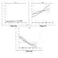
- the evolution of the objective function during the procedure of adding models in the calibration process of the numerical model of the reservoir is given on the Figure 2 .
- the darker vertical bars mark the latest simulation of the LHS and each series of model additions. It can thus be seen that, after the first 70 exploration models (LHS), the points added in sets of 10 have 5 first globally low values of the objective function, and then 5 globally higher values.
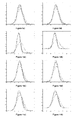
- the figures 3 represent the curves of the a priori distribution, the posterior distribution determined after the initial experimental design and the posterior distribution at the end of the calibration process for each uncertain parameter (MPH2, MPH1, MPV2, MPV1, SORW, SORG, AQUI) and for the objective function (FO).
- the black dot indicates the reference value
- the discontinuous curve in gray corresponds to the prior probability distribution
- the continuous curve in black corresponds to the posterior probability law with 70 models
- the discontinuous curve in black corresponds to to the probability law a posteriori at the end of the calibration process with 210 models.
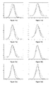
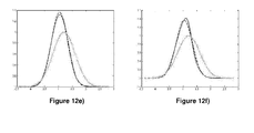
- the black dot designates the reference value
- the gray discontinuous curve which remains horizontal (uniform) corresponds to the prior probability distribution
- the discontinuous curve consisting of a series of small dots corresponds to the probability law a posteriori calculated for two years
- the discontinuous curve consisting of a series of dashes corresponds to the posterior probability distribution calculated for four years
- the continuous curve corresponds to the posterior probability distribution calculated for six years
- the discontinuous curve constituted of a series of lozenges corresponds to the posterior probability law calculated for eight years
- the discontinuous curve consisting of a series of large dots corresponds to the posterior probability law calculated for ten years.
- the posterior analytic law obtained by the method according to the invention requires a computation time of the order of a hundredth of a second, whereas a MCMC sampling of the prior art requires several minutes.
Abstract
Description
La présente invention concerne le domaine technique de l'industrie pétrolière, et plus particulièrement l'exploitation de réservoirs souterrains, tels que des réservoirs pétroliers ou des sites de stockage de gaz.The present invention relates to the technical field of the petroleum industry, and more particularly to the operation of underground reservoirs, such as petroleum reservoirs or gas storage sites.
L'optimisation et l'exploitation d'un gisement pétrolier reposent sur une description aussi précise que possible de la structure, des propriétés pétrophysiques, des propriétés des fluides, etc., du gisement étudié. Pour ce faire, les spécialistes utilisent un outil qui permet de rendre compte de ces aspects de façon approchée : le modèle de réservoir. Un tel modèle constitue une maquette du sous-sol, représentative à la fois de sa structure et de son comportement. Généralement, ce type de maquette est représenté sur un ordinateur, et l'on parle alors de modèle numérique. Un modèle de réservoir comporte un maillage ou grille, généralement tridimensionnelle, associée à une ou plusieurs cartes de propriétés pétrophysiques (porosité, perméabilité, saturation...). L'association consiste à attribuer des valeurs de ces propriétés pétrophysiques à chacune des mailles de la grille.The optimization and exploitation of a petroleum deposit is based on as precise a description as possible of the structure, the petrophysical properties, the properties of the fluids, etc., of the deposit studied. To do this, the specialists use a tool that allows these aspects to be accounted for in an approximate way: the reservoir model. Such a model is a model of the subsoil, representative of both its structure and its behavior. Generally, this type of model is represented on a computer, and one speaks then of numerical model. A reservoir model comprises a mesh or grid, generally three-dimensional, associated with one or more petrophysical property maps (porosity, permeability, saturation, etc.). The association consists of assigning values of these petrophysical properties to each grid cell.
Ces modèles bien connus et largement utilisés dans l'industrie pétrolière, permettent de déterminer de nombreux paramètres techniques relatifs à l'étude ou l'exploitation d'un réservoir, d'hydrocarbures par exemple. En effet, puisque le modèle de réservoir est représentatif de la structure du réservoir et de son comportement, un spécialiste peut l'utiliser par exemple pour déterminer les zones qui ont le plus de chances de contenir des hydrocarbures, les zones dans lesquelles il peut être intéressant/nécessaire de forer un puits d'injection ou de production pour améliorer la récupération des hydrocarbures, le type d'outils à utiliser, les propriétés des fluides utilisés et récupérés.... Ces interprétations de modèles de réservoir en termes de « paramètres techniques d'exploitation » sont bien connues des spécialistes. De la même façon, la modélisation des sites de stockages de CO2 permet de surveiller ces sites, de détecter des comportements inattendus et de prédire le déplacement du CO2 injecté.These well-known models, widely used in the oil industry, make it possible to determine numerous technical parameters relating to the study or the exploitation of a reservoir, of hydrocarbons for example. Indeed, since the reservoir model is representative of the structure of the reservoir and its behavior, a specialist can use it for example to determine the areas that are most likely to contain hydrocarbons, the areas in which it can be interesting / necessary to drill an injection or production well to improve the recovery of hydrocarbons, the type of tools to use, the properties of fluids used and recovered .... These interpretations of reservoir models in terms of "parameters operating techniques "are well known to specialists. Similarly, the modeling of CO 2 storage sites makes it possible to monitor these sites, to detect unexpected behaviors and to predict the displacement of the injected CO 2 .
Afin de réaliser ces différentes interprétations, les spécialistes ont besoin de connaître le comportement dynamique de leur modèle de réservoir. Ceci est réalisé en simulant les écoulements de fluides au sein d'un réservoir au moyen d'un logiciel appelé simulateur d'écoulement. C'est ce qui est appelé une simulation de réservoir. Une ou plusieurs simulations de réservoir peuvent être nécessaires. Le logiciel PumaFlow ® (IFP Energies nouvelles, France) est un exemple de simulateur d'écoulement utilisé dans le domaine de l'exploitation des réservoirs souterrains.In order to realize these different interpretations, the specialists need to know the dynamic behavior of their reservoir model. This is achieved by simulating the flow of fluids within a reservoir using software called flow simulator. This is called a tank simulation. One or more reservoir simulations may be required. The PumaFlow ® software (IFP Energies nouvelles, France) is an example of a flow simulator used in the field of underground reservoir operation.
Ces interprétations sont réalisées à l'aide d'un modèle de réservoir que l'on souhaite le plus représentatif possible, c'est-à-dire cohérent avec toutes les données disponibles. Ces données comprennent en général :
- des mesures en certains points de la formation géologique de la propriété modélisée, par exemple dans des puits. Ces données sont dites statiques car elles sont invariables dans le temps (à l'échelle des temps de la production du réservoir) et sont directement liées à la propriété d'intérêt, et
- des "données d'historique", comprenant des données de production, par exemple les débits de fluide mesurés aux puits ou les concentrations de traceurs et des données issues de campagnes d'acquisition sismique répétées à des temps successifs, dites de sismique 4D. Ces données sont dites dynamiques car elles évoluent en cours d'exploitation et sont indirectement liées aux propriétés attribuées aux mailles du modèle de réservoir.
- measurements at certain points of the geological formation of the modeled property, for example in wells. These data are said to be static because they are invariable in time (at the time scale of the production of the reservoir) and are directly related to the property of interest, and
- "Historical data", including production data, for example fluid flow rates measured at wells or tracer concentrations and data from repeated seismic acquisition campaigns at successive times, called 4D seismic. These data are said to be dynamic because they evolve during operation and are indirectly related to the properties assigned to the meshes of the reservoir model.
Le nombre de données statiques disponibles étant très faible par rapport au nombre de mailles du modèle de réservoir, des extrapolations sont nécessaires. Par exemple des méthodes probabilistes peuvent être utilisées pour remplir le modèle en propriétés pétrophysiques. Dans ce cas les données statiques disponibles sont utilisées pour définir des fonctions aléatoires pour chaque propriété pétrophysique comme la porosité ou la perméabilité. Une représentation de la répartition spatiale d'une propriété pétrophysique est une réalisation d'une fonction aléatoire. De façon générale, une réalisation est générée à partir d'une part d'une moyenne, d'une variance et d'une fonction de covariance qui caractérise la variabilité spatiale de la propriété étudiée et d'autre part d'un germe ou d'une série de nombres aléatoires. De nombreuses techniques de simulation, dites simulations géostatistiques, existent comme la méthode de simulation séquentielle Gaussienne, la méthode de Cholesky ou encore la méthode de transformée de Fourier rapide avec moyenne mobile FFT-MA. Ces techniques sont décrites notamment dans les documents suivants :
-
Goovaerts,P., 1997, Geostatistics for natural resources evaluation, Oxford Press, New York, 483 p -
Le Ravalec, M., Noetinger B., and Hu L.-Y., 2000, The FFT moving average (FFT-MA) generator: an efficient numerical method for generating and conditioning Gaussian simulations, Mathematical Geology, 32(6), 701-723
-
Goovaerts, P., 1997, Geostatistics for Natural Resources Evaluation, Oxford Press, New York, 483 p -
Ravalec, M., Noetinger B., and Hu L.-Y., 2000, The FFT moving average (FFT-MA) generator: an efficient numerical method for generating and conditioning Gaussian simulations, Mathematical Geology, 32 (6), 701-723
La construction d'un modèle de réservoir représentatif se fait par étapes. Tout d'abord, on construit un modèle de réservoir sur la base des données statiques. Puis ce modèle est mis à jour afin de reproduire au mieux les données d'historique via la simulation d'écoulement tout en conservant la cohérence avec les données statiques.The construction of a representative reservoir model is done in stages. First, we build a reservoir model based on static data. Then this model is updated to best reproduce historical data via flow simulation while maintaining consistency with static data.
Les techniques d'intégration des données dynamiques (données de production et/ou sismique 4D) dans un modèle de réservoir sont bien connues des spécialistes : ce sont des techniques dites de "calage d'historique" ("history-matching" en anglais).The techniques of dynamic data integration (4D production and / or seismic data) in a reservoir model are well known to specialists: they are so-called "history-matching" techniques. .
Le calage d'historique consiste à modifier les paramètres d'un modèle de réservoir, tels que les perméabilités, les porosités ou les skins de puits (représentant les endommagements autour du puits), les connections de failles..., pour minimiser les écarts entre les données d'historique mesurées et les réponses correspondantes simulées à partir du modèle de réservoir. Les paramètres peuvent être liés à des régions géographiques comme les perméabilités ou porosités autour d'un puits ou plusieurs puits. L'écart entre les données d'historique et réponses simulées forme une fonctionnelle, dite fonction objectif. Le problème du calage d'historique se résout en minimisant cette fonctionnelle.History calibration consists of modifying the parameters of a reservoir model, such as permeabilities, porosities or well skins (representing the damage around the well), fault connections ..., to minimize the differences between the measured history data and the corresponding responses simulated from the reservoir model. Parameters may be related to geographic areas such as permeabilities or porosities around a well or several wells. The gap between the historical data and the simulated answers forms a functional, called objective function. The problem of history matching is solved by minimizing this functional.
Plusieurs types de méthodes existent pour minimiser cette fonctionnelle. Certaines ne fournissent qu'un seul modèle correspondant au minimum de la fonction objectif. D'autres cherchent à estimer la loi de distribution des paramètres incertains conditionnée aux données dynamiques, dites loi a posteriori, et ainsi estimer l'incertitude sur les paramètres. En effet, l'incertitude sur les données mesurées et le simulateur d'écoulement se propage sur l'estimation du "meilleur" modèle de réservoir. Il est alors important de connaître la loi a posteriori autour du meilleur modèle. Dans le cas général, cette loi ne peut être connue qu'en générant un échantillon de valeurs suivant celle loi. On peut utiliser pour cela des méthodes de type Markov-Chain Monte Carlo (MCMC), qui convergent vers la loi voulue. Une telle méthode est décrite dans le document :
-
Geyer C J (1992) Practical Markov chain Monte Carlo (with discussion). Statistical Science 7:473-511
-
Geyer CJ (1992) Practical Markov Chain Monte Carlo (with discussion). Statistical Science 7: 473-511
Les méthodes MCMC nécessitent un grand nombre de simulations d'écoulement, ce qui demande un temps de calcul important. Pour limiter l'utilisation du simulateur d'écoulement et donc pour réduire le temps de calcul, d'autres solutions ont été imaginées. Par exemple, il est possible d'utiliser un modèle de la fonction objectif dans l'espace des paramètres, appelé "surface de réponse". Ce modèle est construit progressivement au cours des itérations par interpolation des points simulés. Par exemple, le document suivant décrit une telle méthode :
-
Busby D, Feraille M (2008) Adaptive Design of Experiments for Bayesian Inversion - An Application to Uncertainty Quantification of a Mature Oil Field. Journal of Physics: Conference Series 135
-
Busby D, Feraille M (2008) Adaptive Design of Experiments for Bayesian Inversion - An Application to Uncertainty Quantification of a Mature Oil Field. Journal of Physics: Conference Series 135
Cette approche présente donc deux niveaux d'approximation : le premier concerne la convergence de l'algorithme MCMC dont il est très difficile de dire s'il a convergé vers la loi voulue ; le second concerne l'approximation de la fonction objectif par la surface de réponse.This approach therefore has two levels of approximation: the first concerns the convergence of the MCMC algorithm, of which it is very difficult to say whether it has converged towards the desired law; the second concerns the approximation of the objective function by the response surface.
Ainsi, l'objet de l'invention concerne un procédé d'exploitation d'un réservoir géologique selon un schéma d'exploitation défini à partir d'un modèle de réservoir. Le modèle de réservoir est obtenu par une technique de "calage d'historique" probabiliste prenant en compte une loi analytique de distribution conditionnelle de paramètres incertains associée à une surface de réponse donnée. Dans le procédé selon l'invention, cette surface de réponse n'approche pas la fonction objectif elle-même mais une autre fonction déterminée à partir de la fonction objectif. Ceci permet d'obtenir de meilleures approximations de la fonction objectif et donc de la loi a posteriori. De plus, l'utilisation d'une loi analytique permet de réduire les temps de calcul, d'envisager un traitement beaucoup plus rapide des résultats et d'obtenir un modèle de réservoir représentatif en limitant les approximations.Thus, the object of the invention relates to a method of operating a geological reservoir according to an exploitation scheme defined from a reservoir model. The reservoir model is obtained by a probabilistic "history calibration" technique taking into account an analytical law of conditional distribution of uncertain parameters associated with a given response surface. In the method according to the invention, this response surface does not approach the objective function itself but another function determined from the objective function. This makes it possible to obtain better approximations of the objective function and thus of the posterior law. Moreover, the use of an analytical law makes it possible to reduce the calculation times, to consider a much faster processing of the results and to obtain a representative reservoir model by limiting the approximations.
L'invention concerne un procédé d'exploitation d'un réservoir géologique selon un schéma d'exploitation défini à partir d'un modèle de réservoir, ledit modèle de réservoir comportant un maillage associé à des paramètres θ dudit réservoir. Pour ce procédé, on réalise les étapes suivantes :
- a) on construit un modèle de réservoir calé sur des données mesurées au sein dudit réservoir au moyen des étapes suivantes :
- i) on génère de manière stochastique un ensemble initial de modèles de réservoir à partir de lois de probabilité p(θ) desdits paramètres θ ;
- ii) on détermine une fonction objectif F(θ) mesurant un écart entre des données dynamiques y 1,...,yn acquises en cours d'exploitation et des données dynamiques simulées au moyen d'un simulateur d'écoulement et desdits modèles de réservoir appartenant audit ensemble ;
- iii) on détermine à partir de ladite fonction objectif F(θ) une loi analytique p(θ|y 1,...,yn ) de probabilité conditionnelle des paramètres θ connaissant lesdites données dynamiques mesurées y 1,...,yn ;
- iv) on génère au moins un nouveau modèle de réservoir au moyen de ladite loi analytique p(θ|y 1,..., yn ) et on ajoute ledit nouveau modèle audit ensemble de modèles de réservoir ;
- v) on réitère les étapes ii) à iv) et on détermine le modèle de réservoir qui minimise ladite fonction objectif ;
- b) on détermine un schéma d'exploitation optimal du réservoir en simulant l'exploitation du réservoir au moyen dudit modèle de réservoir calé et dudit simulateur d'écoulement ; et
- c) on exploite ledit réservoir en mettant en oeuvre ledit schéma d'exploitation optimal. Selon l'invention, on détermine ladite loi analytique conditionnelle p(θ|y 1,...,yn ) en déterminant une approximation d'une fonction G(θ) telle que G(θ)=exp(-F(θ)), puis en calculant ladite loi analytique à partir de la relation suivante :
-

- a) a reservoir model calibrated on measured data within said reservoir is constructed by the following steps:
- i) stochastically generating an initial set of reservoir models from probability distributions p (θ) of said parameters θ;
- ii) determining an objective function F (θ) measuring a difference between dynamic data y 1 , ..., y n acquired during operation and dynamic data simulated by means of a flow simulator and said models tank belonging to said set;
- iii) determining from said objective function F (θ) an analytic law p (θ | y 1 , ..., y n ) of conditional probability of the parameters θ knowing said measured dynamic data y 1 , ..., y n ;
- iv) generating at least one new reservoir model by means of said analytic law p (θ | y 1 , ..., y n ) and adding said new model to said set of reservoir models;
- v) repeating steps ii) to iv) and determining the reservoir model that minimizes said objective function;
- b) determining an optimal exploitation scheme of the reservoir by simulating the exploitation of the reservoir by means of said model of stalled reservoir and said flow simulator; and
- c) the reservoir is exploited by implementing said optimal exploitation scheme. According to the invention, said conditional analytic law p (θ | y 1 , ..., y n ) is determined by determining an approximation of a function G (θ) such that G (θ) = exp (- F (θ) )), then calculating said analytic law from the following relation:
-
De préférence, on détermine l'approximation de ladite fonction G(θ) en calculant G(θ i ) = exp(-F(θ i )) pour les modèles i appartenant audit ensemble, puis par interpolation desdites valeurs de G(θ i ).Preferably, the approximation of said function G (θ) is determined by calculating G (θ i ) = exp ( -F (θ i )) for the models i belonging to said set, and then interpolating said values of G (θ i ).
Selon un mode de réalisation de l'invention, on interpole lesdites valeurs de G(θ i ) par une technique de krigeage.According to one embodiment of the invention, said values of G (θ i ) are interpolated by a kriging technique.
Selon l'invention, à l'étape iv) à chaque itération on génère plusieurs nouveaux modèles de réservoir, parmi lesquels on choisit M 1 modèles qu'on ajoute audit ensemble, ledit ensemble de modèles de réservoir est constitué lors de la construction de l'ensemble initial d'un nombre M 0 de modèles.According to the invention, in step iv) at each iteration, several new reservoir models are generated, from which M 1 models are selected that are added to said set, said set of reservoir models is constituted during the construction of the reservoir. initial set of a number M 0 of models.
De manière avantageuse, lesdits M 0 modèles dudit ensemble initial sont échantillonnés par une technique de plan d'expériences de type hypercube latin.Advantageously, said M 0 models of said initial set are sampled by a Latin hypercube type experiment plane technique.
De manière avantageuse, lesdits M 1 modèles ajoutés dans ledit ensemble sont choisis à l'aide de l'approximation de ladite fonction G(θ).Advantageously, said model M 1 added in said set are chosen using the approximation of said function G (θ).
Selon une variante de réalisation de l'invention, au moins une partie desdits M 1 modèles sont les modèles pour lesquels l'approximation de la fonction G(θ) donne les valeurs maximales.According to an alternative embodiment of the invention, at least a part of said model M 1 are the models for which the approximation of the function G (θ) gives the maximum values.
En outre, au moins une partie desdits M 1 modèles peuvent être les modèles pour lesquelles pour lesquels la qualité de l'approximation de la fonction G(θ) possède des variances de krigeage les plus élevées parmi lesdits nouveaux modèles.In addition, at least a portion of said model M 1 may be the models for which the quality of the approximation of the function G (θ) has the highest kriging variances among the said new models.
On peut réaliser une étude de sensibilité par le calcul de plusieurs fonctions objectif, chaque fonction objectif étant calculée pour une partie des paramètres ou pour un intervalle de temps limité par rapport aux informations disponibles.A sensitivity study can be performed by calculating several objective functions, each objective function being calculated for a part of the parameters or for a limited time interval with respect to the information available.
L'invention concerne également un produit programme d'ordinateur téléchargeable depuis un réseau de communication et/ou enregistré sur un support lisible par ordinateur et/ou exécutable par un processeur. Il comprend des instructions de code de programme pour la mise en oeuvre du procédé tel que décrit ci-dessus, lorsque ledit programme est exécuté sur un ordinateur.The invention also relates to a computer program product downloadable from a communication network and / or recorded on a computer readable medium and / or executable by a processor. It includes program code instructions for carrying out the method as described above, when said program is run on a computer.
D'autres caractéristiques et avantages du procédé selon l'invention, apparaîtront à la lecture de la description ci-après d'exemples non limitatifs de réalisations, en se référant aux figures annexées et décrites ci-après.
- La
figure 1 illustre les différentes étapes du procédé selon l'invention. - La
figure 2 illustre des valeurs de la fonction objectif pour les différents modèles de réservoir considérés au cours du processus de calage du procédé selon l'invention. - Les
figures 3 illustrent la distribution de différents paramètres. - Les
figures 4 illustrent la distribution de différents paramètres pour différentes périodes de calage. - Les
figures 5 illustrent la distribution de différents paramètres lorsque certains paramètres sont fixés. - Les
figures 6 illustrent des données de production au puits. - Les
figures 7 à 12 illustrent la distribution de différents paramètres pourl'exemple 2.
- The
figure 1 illustrates the different steps of the method according to the invention. - The
figure 2 illustrates values of the objective function for the different reservoir models considered during the calibration process of the method according to the invention. - The
figures 3 illustrate the distribution of different parameters. - The
figures 4 illustrate the distribution of different parameters for different timing periods. - The
figures 5 illustrate the distribution of different parameters when certain parameters are fixed. - The
figures 6 illustrate well production data. - The
Figures 7 to 12 illustrate the distribution of different parameters for example 2.
Le procédé de l'invention est destiné à l'exploitation d'un réservoir souterrain, cette exploitation peut consister à la récupération d'hydrocarbures mais aussi au stockage de gaz, tel que du CO2 dans le réservoir. Dans la suite de la description, nous allons décrire essentiellement l'utilisation du procédé dans le cas de la récupération d'hydrocarbures.The method of the invention is intended for the exploitation of an underground reservoir, this operation may consist of the recovery of hydrocarbons but also the storage of gas, such as CO 2 in the reservoir. In the remainder of the description, we will essentially describe the use of the process in the case of hydrocarbon recovery.
La
- 1) détermination de paramètres incertains (X1)
- 2) construction d'un ensemble initial de modèles de réservoir (EMRi)
- 3) calage d'historique de type probabiliste (CAL)
- 4) simulation de schémas d'exploitation (SE)
- 5) exploitation du gisement (EX)
- 1) determination of uncertain parameters (X1)
- 2) Construction of an initial set of reservoir models (EMRi)
- 3) Probabilistic type history (CAL) calibration
- 4) Simulation of exploitation plans (SE)
- 5) exploitation of the deposit (EX)
Lors de cette étape, on détermine un ensemble de P paramètres incertains θ = (θ1...θ P ) utilisés dans le modèle de réservoir ainsi que des lois de probabilité p(θ i ) (dites lois "a priori") pour chacun de ces paramètres. Ces lois n'incorporent aucune information venant des données dynamiques. Elles sont basées sur des informations venant de la connaissance du réservoir, de données statiques (géologiques par exemple), etc. Par exemple, les lois de probabilité p(θ) choisies peuvent être du type uniforme, Gaussien, etc.During this step, we determine a set of P uncertain parameters θ = (θ 1 ... θ P ) used in the reservoir model as well as probability laws p (θ i ) (so-called "prior" laws) for each of these parameters. These laws do not incorporate any information from dynamic data. They are based on information coming from tank knowledge, static data (geological data for example), etc. For example, the laws of probability p (θ) chosen can be of the uniform type, Gaussian, etc.
Les paramètres incertains peuvent être liés à n'importe quelle partie du modèle de réservoir. Par exemple, il peut s'agir de paramètres permettant de remplir le modèle de réservoir en propriétés pétrophysiques (perméabilité, porosité), de paramètres caractérisant les puits (skins), les fluides en place ou injectés (saturation en huile résiduelle après balayage à l'eau ou au gaz par exemple) ou encore la structure du réservoir (connections de failles). Un jeu de valeurs des paramètres θ = (θ1...θ P ), qui correspond également à un point de l'espace des paramètres, définit donc un modèle de réservoir. Une modification de chaque paramètre entraîne donc une modification du modèle de réservoir. En particulier, si le paramètre incertain est lié à la répartition spatiale d'une propriété pétrophysique, il peut être nécessaire d'utiliser une technique de simulation géostatistique pour générer le modèle de réservoir associé.The uncertain parameters can be related to any part of the reservoir model. For example, they may be parameters to fill the reservoir model with petrophysical properties (permeability, porosity), parameters characterizing the wells (skins), the fluids in place or injected (saturation with residual oil after sweeping with the water or gas for example) or the tank structure (fault connections). A set of parameter values θ = (θ 1 ... θ P ), which also corresponds to a point in the parameter space, therefore defines a reservoir model. A modification of each parameter therefore leads to a modification of the reservoir model. In particular, if the uncertain parameter is related to the spatial distribution of a petrophysical property, it may be necessary to use a geostatistical simulation technique to generate the associated reservoir model.
Les formations géologiques sont en général des milieux très hétérogènes. La modélisation d'un réservoir, c'est-à-dire la construction d'un modèle de réservoir respectant les données statiques, nécessite de recourir à des procédés de construction dits « probabilistes » du fait de la limitation de l'information disponible (nombre de puits restreints, ...). De ce fait, les modèles géologiques construits à partir de ces procédés probabilistes sont appelés « modèles stochastiques ». La construction d'un modèle stochastique de réservoir doit d'abord dépendre de l'environnement du dépôt géologique, ce qui permet de représenter les hétérogénéités majeures qui contrôlent l'écoulement des fluides. L'intégration des données statiques dans ce modèle passe par des opérations linéaires et peut se faire à partir de techniques géostatistiques bien connues des spécialistes. Pour cela, on peut utiliser avantageusement un simulateur géostatistique.Geological formations are generally very heterogeneous environments. Reservoir modeling, ie the construction of a reservoir model that respects static data, requires the use of so-called "probabilistic" construction processes because of the limited information available ( number of restricted wells, ...). As a result, geological models constructed from these probabilistic processes are called "stochastic models". The construction of a stochastic reservoir model must first depend on the environment of the geological repository, which allows to represent the major heterogeneities that control the flow of fluids. The integration of static data in this model involves linear operations and can be done from geostatistical techniques well known to specialists. For this, one can advantageously use a geostatistical simulator.
Un modèle de réservoir, pouvant être représenté sur un ordinateur, comprend une grille à N dimensions (N>0 et en général égal à deux ou trois) dont chacune des mailles se voit affecter la valeur d'une propriété caractéristique de la zone étudiée. Il peut s'agir par exemple de la porosité ou de la perméabilité distribuée dans un réservoir. Ces valeurs constituent des cartes. Ainsi un modèle comprend une grille associée à au moins une carte. D'autres paramètres caractérisant par exemple les puits ou les fluides injectés interviennent également dans la définition de ce modèle.A reservoir model, which can be represented on a computer, comprises an N-dimensional grid (N> 0 and in general equal to two or three) each of whose meshes is assigned the value of a characteristic property of the zone studied. This may be, for example, the porosity or the permeability distributed in a reservoir. These values constitute maps. Thus a model includes a grid associated with at least one map. Other parameters characterizing for example wells or injected fluids are also involved in the definition of this model.
Lors de cette étape on génère de manière stochastique un ensemble initial de modèles de réservoir au moyen de la loi de probabilité a priori p(θ) de chaque paramètre incertain.During this step, an initial set of reservoir models is generated stochastically by means of the prior probability law p (θ) of each uncertain parameter.
Plus précisément, on génère pour chaque paramètre incertain θ i sélectionné lors de l'étape 1), un échantillon (X1) de M 0 valeurs selon la loi de distribution a priori p(θ i ), par exemple à partir d'une méthode de plan d'expérience de type hypercube latin. On obtient ainsi un ensemble de M 0 jeux de valeurs des paramètres incertains, et donc M 0 modèles de réservoir différents.More precisely, for each uncertain parameter θ i selected in step 1), a sample (X1) of M 0 values according to the prior distribution law p (θ i ) is generated, for example from a method experience plan of the Latin hypercube type. We thus obtain a set of M 0 sets of values of the uncertain parameters, and thus M 0 different reservoir models.
Le but du processus de calage selon l'invention est de construire un modèle de réservoir le plus représentatif possible. Or, à ce stade, les données dynamiques n'ont pas été considérées pour construire le modèle de réservoir initial. On acquiert donc des données dynamiques en cours d'exploitation du gisement (DD). Il s'agit de données de production, d'essais de puits, de temps de percée, de sismique 4D... dont la particularité est de varier au cours du temps en fonction des écoulements de fluide dans le réservoir. Ces mesures sont réalisées au moyen d'outils de mesure tels que des débitmètres ou des capteurs sismiques. On note (y 1...yn ) le vecteur des données dynamiques observées et (t 1...tn ) les temps d'acquisition correspondants.The purpose of the calibration process according to the invention is to construct a reservoir model that is as representative as possible. At this stage, dynamic data has not been considered to build the initial reservoir model. So we acquire dynamic data during the exploitation of the deposit (DD). It is production data, well tests, breakthrough time, 4D seismic ... whose particularity is to vary over time depending on the flow of fluid in the tank. These measurements are made using measuring tools such as flow meters or seismic sensors. We denote ( y 1 ... y n ) the vector of the observed dynamic data and ( t 1 ... t n ) the corresponding acquisition times.
Ces données dynamiques sont ensuite intégrées dans le modèle de réservoir par le biais du calage probabiliste. Selon l'invention, on réalise un calage d'historique de type probabiliste (CAL) en réalisant les étapes suivantes :
- i. on utilise un simulateur d'écoulement f pour calculer la réponse en production simulée avec les modèles de réservoir que l'on souhaite évaluer (SIM) ;
- ii. on calcule une fonction objectif (OF) mesurant l'écart entre les résultats simulés (SIM) et les données dynamiques (DD) associées ;
- iii. on construit par krigeage une approximation de l'exponentielle de l'opposé de la fonction objectif, et on détermine pour cette surface de réponse une loi de probabilité conditionnelle analytique p̃(θ|y 1,..., yn ) des paramètres incertains connaissant les données dynamiques, cette loi est également appelée loi a posteriori (POST) ;
- iv. on génère au moins un nouveau modèle de réservoir que l'on souhaite évaluer pour améliorer la qualité de la surface de réponse (EMR) ;
- v. on réitère les étapes i) à iv), pour connaître le plus précisément possible la distribution a posteriori de la fonction objectif.
- i. a flow simulator f is used to calculate the simulated production response with the reservoir models that are to be evaluated (SIM);
- ii. an objective function (OF) is calculated measuring the difference between the simulated results (SIM) and the associated dynamic data (DD);
- iii. we construct by kriging an approximation of the exponential of the opposite of the objective function, and we determine for this response surface an analytic conditional probability law p (θ | y 1 , ..., y n ) uncertain parameters knowing the dynamic data, this law is also called a posteriori (POST);
- iv. generating at least one new reservoir model that is to be evaluated to improve the quality of the response surface (EMR);
- v. Steps i) to iv) are reiterated to find out as precisely as possible the posterior distribution of the objective function.
Au moyen d'un simulateur d'écoulement, par exemple le logiciel PumaFlow ® (IFP Energies nouvelles, France), on simule les écoulements dans les modèles de réservoir à évaluer, c'est à dire soit les modèles de réservoir de l'ensemble initial, soit les modèles de réservoir générés lors de l'itération précédente. On peut simuler par exemple la récupération de pétrole ou les déplacements des fluides (par exemple les gaz stockés) dans le réservoir.By means of a flow simulator, for example the PumaFlow ® software (IFP Energies nouvelles, France), the flows in the reservoir models to be evaluated are simulated, ie either the reservoir models of the set initial, ie the reservoir models generated during the previous iteration. For example, the recovery of oil or the displacements of the fluids (for example the gases stored) can be simulated in the tank.
La fonction objectif F(θ) représente les écarts entre les données dynamiques mesurées (DD) et les données dynamiques simulées (SIM). Selon un mode de réalisation de l'invention, on calcule la fonction objectif F(θ) au sens des moindres carrés : 
Selon l'invention, on calcule la fonction objectif pour chaque modèle de réservoir de l'ensemble. On rappelle que cet ensemble comporte initialement M = M 0 modèles de réservoir. Cet ensemble augmente à chaque itération d'un nombre M 1 de modèles. La sélection des M 1 modèles supplémentaires, ou de façon équivalente des M 1 jeux de valeurs des paramètres incertains, est décrite dans le paragraphe iv) de sélection de nouveaux modèles de réservoir.According to the invention, the objective function is calculated for each reservoir model of the set. It will be recalled that this set initially comprises M = M 0 reservoir models. This set increases with each iteration of a number M 1 of models. The selection of additional M 1 models, or equivalently M 1 sets of uncertain parameter values, is described in paragraph iv) of selection of new reservoir models.
Le problème inverse en ingénierie de réservoir consiste à chercher la valeur de paramètres incertains du modèle réservoir qui, appliquées au simulateur d'écoulement, fournissent une réponse simulée la plus proche possible des données dynamiques mesurées. La réponse simulée aux puits se modélise de la façon suivante : ![]()
où ti est le i-ième temps d'acquisition de données dynamiques, yi le vecteur des données dynamiques observées, θ le vecteur des paramètres incertains du modèle, f le simulateur d'écoulement qui modélise la relation entre les paramètres et les données observées, ε i l'erreur entre le modèle et la donnée dynamique et n le nombre de données dynamiques mesurées. L'objectif est d'utiliser les données observées pour déduire des informations sur le vecteur des paramètres incertains θ.The inverse problem in reservoir engineering is to look for the value of uncertain parameters of the reservoir model that, applied to the flow simulator, provide a simulated response as close as possible to the measured dynamic data. The simulated well response is modeled as follows: ![]()
where t i is the i th dynamic data acquisition time, y i the vector of the observed dynamic data, θ the vector of the uncertain parameters of the model, f the flow simulator which models the relationship between the parameters and the data observed, ε i the error between the model and the dynamic data and n the number of dynamic data measured. The objective is to use the observed data to derive information on the vector of the uncertain parameters θ.
On suppose ici que les erreurs ε i entre le modèle de simulation d'écoulement f(ti ,θ) et les données observées yi suivent une loi donnée, estimée en fonction des erreurs de mesure. La loi de distribution conditionnelle du vecteur θ connaissant les données mesurées, ou loi a posteriori, est donnée par la formule de Bayes : 
où p(θ) est la loi de distribution a priori, p(y 1,...,yn ) est la loi de distribution des données, p(y 1,...,yn |θ) est la loi de distribution conditionnelle des données dynamiques sachant θ et p(θ|(y 1,...,yn ) est la loi de distribution conditionnelle a posteriori recherchée.It is assumed here that the errors ε i between the flow simulation model f ( t i , θ) and the observed data y i follow a given law, estimated as a function of the measurement errors. The conditional distribution law of the vector θ knowing the measured data, or posterior law, is given by the Bayes formula:
where p (θ) is the distribution law a priori, p ( y 1 , ..., y n ) is the distribution law of the data, p ( y 1 , ..., y n | θ) is the law conditional distribution of dynamic data knowing θ and p (θ | ( y 1 , ..., y n ) is the conditional posterior distribution law sought.
Enfin, en supposant les erreurs ε i Gaussiennes et indépendantes, la loi a posteriori peut se réécrire : 
Et dans ce cas, le poids ω i utilisé pour le calcul de la fonction objectif est défini par ![]()
![]()
![]()
![]()
Selon l'invention, on détermine une approximation de la loi p(θ|(y 1,...,yn ) de distribution conditionnelle des paramètres incertains connaissant les données dynamiques mesurées par une loi analytique p̃(θ|(y 1,...,yn ) dépendant de la fonction objectif F(θ).According to the invention, an approximation of the conditional distribution law p (θ | ( y 1 , ..., y n ) of the uncertain parameters knowing the dynamic data measured by an analytic law p (θ | ( y 1 , ..., y n ) depending on the objective function F (θ).
On détermine ladite loi analytique conditionnelle p̃(θ|(y 1,...,yn ) en considérant une fonction G(θ) dépendante de ladite fonction objectif F(θ), définie par G(θ) = exp(-F(θ)). La loi a posteriori se réécrit alors : 

La fonction G(θ) n'étant pas connue de manière analytique, on en construit une approximation, appelée également surface de réponse, par interpolation des valeurs connues G(θ j )=exp(-F(θ j )) calculées pour chacun des modèles j de réservoir au cours de l'étape ii). Contrairement à l'art antérieur, la surface de réponse utilisée par l'invention approche non pas la fonction objectif, mais une fonction dépendant de cette fonction objectif. La fonction G(θ) est comprise entre 0 et 1, et varie donc dans un intervalle plus restreint que la fonction F(θ). Par conséquent, il est plus facile de construire une bonne approximation de la fonction G(θ) que de la fonction F(θ).Since the function G (θ) is not known analytically, we construct an approximation, also called a response surface, by interpolation of the known values G (θ j ) = exp ( -F (θ j )) calculated for each reservoir models in step ii). Unlike the prior art, the response surface used by the invention approaches not the objective function, but a function dependent on this objective function. The function G (θ) is between 0 and 1, and therefore varies in a narrower range than the function F (θ). Consequently, it is easier to construct a good approximation of the function G (θ) than of the function F (θ).
De préférence, la méthode d'interpolation utilisée est une technique de krigeage ou toute autre méthode de régression appartenant à la famille de la minimisation du risque empirique pénalisé dans des espaces de Hilbert à noyau reproduisant (RKHS de l'anglais Reproducting Kernel Hilbert Space). Ces méthodes d'interpolation permettent d'écrire l'approximation de la fonction (ou surface de réponse) G̋(θ) sous la forme d'une combinaison linéaire de fonctions connues. Le calcul de la loi p̃(θ|y 1,...,yn ) de probabilité conditionnelle associée à G̋(θ) fait alors intervenir différentes intégrales de ces fonctions connues, qui sont calculables analytiquement.Preferably, the interpolation method used is a kriging technique or any other regression method belonging to the family of penalized empirical risk minimization in reproducing kernel Hilbert spaces (RKHS of the English Reproducting Kernel Hilbert Space). . These interpolation methods make it possible to write the approximation of the function (or response surface) G̋ (θ) in the form of a linear combination of known functions. The calculation of the conditional probability law p (θ | y 1 , ..., y n ) associated with G̋ (θ) then involves different integrals of these known functions, which are analytically computable.
On génère de nouveaux modèles de réservoir, c'est à dire de nouveaux jeux de valeurs des paramètres incertains, en fonction de la loi analytique p̃(θ|y 1,...,yn ) de probabilité conditionnelle obtenue à l'étape précédente. On sélectionne M 1 modèles parmi cet échantillon pour lesquels on va calculer la fonction objectif afin d'améliorer notre connaissance de cette fonction, et donc la qualité de la surface de réponse.New reservoir models are generated, that is to say new sets of uncertain parameter values, as a function of the analytic law p (θ | y 1 , ..., y n ) of conditional probability obtained at step previous. We select M 1 models among this sample for which we will calculate the objective function to improve our knowledge of this function, and thus the quality of the response surface.
Selon l'invention, l'ensemble des modèles de réservoir pour lesquels on calcule la réponse en production est augmenté à chaque itération du processus de calage par l'ajout de M 1 nouveaux modèles. Ces modèles sont choisis selon plusieurs critères (de préférence avec un nombre de modèles identique pour chacun des critères), notamment :
- (i) on sélectionne les points de l'espace des paramètres, c'est à dire les jeux de valeur des paramètres incertains, pour lesquels la qualité de l'approximation de la fonction G(θ) est faible.
- (ii) on sélectionne les points de l'espace des paramètres pour lesquels la surface de réponse G̃(θ) prédit de fortes valeurs, c'est-à-dire de faibles valeurs de la fonction objectif. On peut par exemple utiliser la technique de l'Expected Improvement (amélioration attendue) décrite par exemple dans le document :
Schonlau M (1997) Computer Experiments and Global Optimization, Dissertation, University of Waterloo, Canada
- (i) we select the points of the parameter space, ie the sets of values of the uncertain parameters, for which the quality of the approximation of the function G (θ) is low.
- (ii) we select the points of the parameter space for which the response surface G (θ) predicts high values, that is, small values of the objective function. One can for example use the technique of the Expected Improvement described for example in the document:
Schonlau M (1997) Computer Experiments and Global Optimization, Dissertation, University of Waterloo, Canada
D'autres critères peuvent être utilisés notamment pour choisir des points où la variance de krigeage est élevée, les points qui si on les ajoute font diminuer le plus l'intégrale de l'erreur de modèle, ou les points d'entropie maximale, ....Other criteria can be used in particular to choose points where the kriging variance is high, the points which, if they are added, decrease the integral of the model error, or the maximum entropy points, the most. ...
On génère ensuite les modèles de réservoir correspondant à chaque nouveau jeu de valeurs des paramètres sélectionnés précédemment. Ceci peut nécessiter d'utiliser un simulateur géostatistique pour générer les propriétés pétrophysiques du modèle de réservoir.The reservoir models corresponding to each new set of values of the previously selected parameters are then generated. This may require the use of a geostatistical simulator to generate the petrophysical properties of the reservoir model.
Tant que le nombre maximum de points que l'on peut évaluer (simuler) n'a pas été atteint, on réitère les étapes du calage avec un nombre de modèles de réservoir appartenant à l'ensemble de plus en plus important.As long as the maximum number of points that can be evaluated (simulate) has not been reached, the calibration steps are reiterated with a number of reservoir models belonging to the increasingly important set.
A chaque construction par krigeage de G̃(θ), on calcule le critère de qualité Q2 de cette surface de réponse à partir des modèles de réservoir de l'ensemble utilisé pour la définir : 
Dans le cas déterministe, un modèle de réservoir calé avec les données dynamiques revient à associer aux paramètres incertains (ou de calage du modèle) la valeur correspondant à la plus faible valeur de la fonction objectif. Dans notre cas, un modèle de réservoir calé avec les données dynamiques et selon la méthode probabiliste décrite précédemment revient à associer aux paramètres incertains (ou de calage du modèle) leur loi de probabilité a posteriori.In the deterministic case, a reservoir model calibrated with the dynamic data amounts to associating with the uncertain parameters (or calibration of the model) the value corresponding to the lowest value of the objective function. In our case, a model of reservoir calibrated with the dynamic data and according to the probabilistic method described previously amounts to associating with the uncertain parameters (or calibration of the model) their posterior probability law.
Selon un mode de réalisation de l'invention, on utilise une fonction objectif normalisée 

A partir d'au moins un modèle de réservoir calé de manière probabiliste, les spécialistes peuvent déterminer plusieurs schémas d'exploitation (SE) correspondant à différentes options possibles d'exploitation du réservoir souterrain : emplacement des puits producteur et/ou injecteur, valeurs cibles pour les débits par puits et/ou pour le réservoir, le type d'outils utilisés, les fluides utilisés et récupérés... Pour chacun de ces schémas, il convient de déterminer leurs prévisions de production après la période de calage. Ces prévisions de production probabilistes sont obtenues au moyen d'un logiciel de simulateur d'écoulement (de préférence le même que celui utilisé auparavant) ainsi qu'au moyen du modèle numérique de réservoir calé.From at least one tank model calibrated in a probabilistic manner, the specialists can determine several exploitation plans (SE) corresponding to different possible options for the exploitation of the underground reservoir: location of the wells producer and / or injector, target values for the flows per well and / or for the reservoir, the type of tools used, the fluids used and recovered ... For each of these schemes, it is necessary to determine their production forecasts after the calibration period. These probabilistic production forecasts are obtained by means of flow simulator software (preferably the same as that used previously) as well as by means of the calibrated reservoir model.
On définit un ou plusieurs schémas d'exploitation (SE) possibles adaptés au modèle de réservoir. Pour chacun de ces schémas, on propage l'incertitude a posteriori obtenue après le calage probabiliste.One or more possible exploitation schemes (SE) are defined that are adapted to the reservoir model. For each of these schemes, the posterior uncertainty obtained after the probabilistic calibration is propagated.
La propagation de la loi a posteriori des paramètres incertains peut être réalisée en construisant des surfaces de réponses sur les résultats d'intérêts de la simulation (débit cumulé d'huile ou valeur économique du réservoir, par exemple), ceci afin d'éviter le lancement d'un trop grand nombre de simulations numériques. La description de cette étape est donnée par exemple dans le document :
-
Feraille M, Marrel A (2012) Prediction under uncertainty on a mature field. Oil & Gas Science and Technology
-
Feraille M, Marrel A (2012) Prediction under uncertainty on a mature field. Oil & Gas Science and Technology
A partir des prévisions de productions probabilistes définies pour chaque schéma d'exploitation (étape précédente), les spécialistes peuvent par comparaison choisir le schéma d'exploitation qui leur semble le plus pertinent. Par exemple :
- en comparant le maximum du volume d'huile récupéré, on peut déterminer le schéma de production susceptible de fournir le maximum de récupération ou d'être le plus rentable.
- en comparant l'écart type du volume d'huile récupéré, on peut déterminer le schéma de production le moins risqué.
- By comparing the maximum volume of oil recovered, we can determine the production scheme that can provide the maximum recovery or be the most profitable.
- by comparing the standard deviation of the volume of oil recovered, the least risky production scheme can be determined.
On exploite alors le réservoir selon le schéma d'exploitation choisi (EX) par exemple en forant de nouveaux puits (producteur ou injecteur), en modifiant les débits et/ou les fluides injectés ...The reservoir is then exploited according to the chosen exploitation scheme (EX), for example by drilling new wells (producer or injector), by modifying the flows and / or the injected fluids.
Le calcul analytique, donc quasi-instantané, des lois de probabilité a posteriori des paramètres et de la fonction objectif pour une surface de réponse donnée permet d'envisager de nouvelles voies d'exploitation des résultats du calage probabiliste permettant de mieux comprendre l'impact de chaque paramètre incertain sur le comportement du réservoir.The quasi-instantaneous analytical calculation of the posterior probability distributions of the parameters and of the objective function for a given response surface allows to consider new ways of exploiting probabilistic calibration results to better understand the impact of each uncertain parameter on reservoir behavior.
Par exemple, on peut décider de fixer la valeur d'un ou plusieurs des paramètres et de regarder l'impact sur l'incertitude des autres paramètres ainsi que sur la ou les fonctions objectif choisies. Dans ce cas, il suffit de recalculer analytiquement la loi de distribution conditionnelle des paramètres θ j, j = 1...N, j ≠ i conditionnée à la valeur choisie pour θ i .For example, one may decide to set the value of one or more of the parameters and look at the impact on the uncertainty of the other parameters as well as on the objective function (s) chosen. In this case, it suffices to recalculate analytically the conditional distribution law of the parameters θ j , j = 1 ... N, j ≠ i conditioned to the value chosen for θ i .
On peut également envisager de considérer plusieurs fonctions objectif selon l'information recherchée. Ceci se fait en estimant la distribution a posteriori des paramètres pour chacune de ces fonctions via la construction d'une surface de réponse. La fonction objectif F mesure l'écart global entre les résultats de simulations et les données dynamiques mesurées. Cette fonction est classiquement construite au sens des moindres carrés. D'un point de vue métier, une fonction objectif calcule la somme des écarts entre des propriétés d'historique liées à des objets métiers (puits P1 à P10, groupe de puits, piège, ...), eux-mêmes liés à des propriétés comme le débit d'huile QOS, d'eau QWS, de gaz QGS, ..., qui sont elles-mêmes fonction du temps où ont été effectuées les mesures (par exemple tous les mois de 1980 à 2000). A partir des données d'historique, il est donc possible de calculer une fonction objectif pour n'importe quel sous-ensemble constitué d'une partie des objets, des propriétés ou d'un certain nombre d'intervalles de temps. Par exemple, on peut déterminer une fonction objectif liée :
- au puits P1 pour toutes les propriétés et tous les temps, ou
- à la période 1980-1990 pour tous les objets et toutes les propriétés.
- at well P1 for all properties and all times, or
- in the period 1980-1990 for all objects and properties.
Il peut donc être intéressant de connaître l'influence des paramètres sur différentes fonctions objectif, par exemple :
- pour identifier à partir de quel moment les différents paramètres deviennent influents, il suffit de considérer, pour plusieurs temps, la fonction objectif incluant toutes les données jusqu'à chacun de ces temps, puis de construire une surface de réponse pour chacune des fonctions obtenues. On a ainsi accès à l'évolution de la distribution a posteriori en fonction du temps de calage de manière interactive.
- pour connaître l'influence des paramètres sur chaque puits, il suffit d'estimer les distributions a posteriori des fonctions objectif associées aux propriétés d'un puits donné.
- to identify from which moment the various parameters become influential, it suffices to consider, for several times, the objective function including all the data up to each of these times, and then to construct a response surface for each of the functions obtained. This gives access to the evolution of the posterior distribution as a function of the stalling time interactively.
- to determine the influence of the parameters on each well, it is sufficient to estimate the posterior distributions of the objective functions associated with the properties of a given well.
Connaître l'influence des paramètres incertains sur des fonctions objectif "métiers" définies par le spécialiste lui permet de mieux appréhender le fonctionnement du réservoir et de prendre des décisions. Par exemple, il est possible
- de fixer fictivement la valeur des paramètres vus comme influents, le spécialiste peut alors s'assurer que la réduction de l'incertitude sur le modèle de réservoir qui en découle (sur les autres paramètres et sur une ou plusieurs fonctions objectif définies par l'ingénieur) est suffisante pour justifier une meilleure caractérisation de ces paramètres influents. Dans ce cas, de nouvelles mesures sur le champ pétrolier peuvent être réalisées (tests de puits, diagraphies, ...).
- de savoir que des paramètres liés à une partie du réservoir commencent à avoir une influence à partir d'une date sur une ou des fonctions objectif liées à une autre partie du réservoir, ce qui permet de mieux comprendre le fonctionnement dynamique du réservoir. Cette compréhension peut se traduire par des schémas d'exploitation différents et adaptés pour chacune des parties du réservoir.
- to fictitiously set the value of the parameters seen as influential, the specialist can then ensure that the reduction of the uncertainty on the resulting reservoir model (on the other parameters and on one or more objective functions defined by the engineer ) is sufficient to warrant a better characterization of these influential parameters. In this case, new measurements on the oil field can be made (well tests, logging, ...).
- to know that parameters related to a part of the tank begin to influence from one date on one or objective functions related to another part of the tank, which allows to better understand the dynamic operation of the tank. This understanding can result in different and adapted operating schemes for each part of the tank.
Enfin, on peut envisager des études de sensibilité aux poids de la fonction objectif, ce qui est extrêmement coûteux si l'on doit utiliser la méthode MCMC de l'art antérieur.Finally, one can consider studies of sensitivity to the weight of the objective function, which is extremely expensive if one must use the MCMC method of the prior art.
Afin d'illustrer le procédé selon l'invention, le demandeur a réalisé deux séries d'expérimentations. La première série concerne l'obtention des distributions a posteriori. La deuxième série illustre la bonne corrélation entre la loi analytique associée aux surfaces de réponse et la loi de distribution conditionnelle exacte.In order to illustrate the process according to the invention, the applicant has carried out two series of experiments. The first series concerns the obtaining of posterior distributions. The second series illustrates the good correlation between the analytic law associated with the response surfaces and the exact conditional distribution law.
Pour illustrer la méthode, on décrit un exemple d'application synthétique. Le réservoir considéré contient initialement du gaz, de l'huile et de l'eau. Il est fermé par des failles sur deux côtés, et par un aquifère sur les autres côtés. La production se fait par déplétion à partir de six puits (PRO1 PRO4, PROS, PRO11, PRO12, PRO15) avec un débit de production d'huile de 150 m3/jour imposé à chaque puits producteur pendant 10 ans. Au cours de cette période de production, le cumulé d'huile (V) et le ratio gaz/huile (R) sont collectés pour chaque puits producteur, ainsi que le cumulé d'huile total dans le réservoir. Ces valeurs sont connues avec un bruit relatif de 4%. Ces données sont illustrées par les courbes de la
On suppose également connue dans le réservoir la distribution des propriétés pétrophysiques (porosité, perméabilité). Les paramètres incertains sont les sept paramètres suivants : quatre multiplicateurs de transmissitivité (MPH2, MPH1, MPV2, MPV1), la saturation en huile résiduelle après balayage à l'eau (SORW), la saturation en huile résiduelle après balayage au gaz (SORG) et un paramètre caractérisant l'aquifère (AQUI).The distribution of petrophysical properties (porosity, permeability) is also known in the reservoir. The uncertain parameters are the following seven parameters: four transmissitivity multipliers (MPH2, MPH1, MPV2, MPV1), residual oil saturation after water sweep (SORW), residual oil saturation after gas sweeping (SORG) and a parameter characterizing the aquifer (AQUI).
Il s'agit alors d'estimer, en utilisant le procédé selon l'invention, la distribution des paramètres incertains et la distribution de la fonction objectif conditionnées aux données dynamiques.It is then necessary to estimate, using the method according to the invention, the distribution of the uncertain parameters and the distribution of the objective function conditioned to the dynamic data.
Le calage probabiliste est réalisé avec un plan d'expérience initial de type hypercube latin LHS définissant un ensemble constitué de 70 modèles de réservoir, puis avec un ajout de modèles par séries de 10 à chaque itération du processus de calage. Les 5 premiers modèles ajoutés sont choisis là où la surface de réponse G̃(θ) prédit de fortes valeurs, et les 5 suivants où la qualité de l'approximation de G(θ) est faible au sens de la variance de krigeage élevée. L'évolution de la fonction objectif au cours de la procédure d'ajout de modèles dans le processus de calage du modèle numérique du réservoir est donnée sur la
Les
Grâce à la mise à jour quasi-immédiate (car analytique) de la distribution conditionnelle a posteriori pour un modèle de krigeage donné, on peut envisager de fixer la valeur d'un ou plusieurs des paramètres incertains et de regarder l'impact sur l'incertitude des autres paramètres. Ceci est illustré par exemple sur les
On peut également envisager des études de sensibilité aux poids de la fonction objectif. Par exemple, on peut s'intéresser à l'évolution des lois conditionnelles a posteriori des paramètres lorsque l'on considère un intervalle de calage plus ou moins long dans le calcul de la fonction objectif. Dans le cas présenté ici, on a considéré toutes les simulations effectuées lors du processus probabiliste et reconstruit le modèle de krigeage associé respectivement à un historique de 10, 8, 6, 4 et 2 ans. Les nouvelles lois conditionnelles a posteriori des paramètres sont données sur les
Cet exemple permet de détailler la méthodologie proposée sur un exemple analytique, qui nous permet de valider et d'étudier de manière approfondie les formes analytiques possibles de la loi a posteriori pour différents cas. Tous les exemples développés ici ont été traités avec le logiciel Matlab ® (MathWorks, États-Unis) et la boîte à outils "Dacefit" pour la construction du krigeage.This example allows to detail the proposed methodology on an analytical example, which allows us to validate and study in depth the possible analytical forms of the posterior law for different cases. All the examples developed here have been processed with Matlab ® software (MathWorks, USA) and the "Dacefit" toolbox for building kriging.
Pour cet exemple on remplace le simulateur d'écoulement f par un modèle linéaire ![]()
![]()
Pour tester la méthode de calage du procédé selon l'invention sur ce modèle linéaire, on répète la procédure suivante pour D = 1, D = 2 et D = 3 :
- 1. On fixe la valeur de référence de θ
- 2. On choisit n = 10 points dans l'intervalle [0,1]D selon un hypercube latin, on note ces points ti , i = 1,..,n et on génère les observations


- 3. On génère un ensemble (θ i )i=1,..,N de N paramètres avec N = 10D, 20D, ou 50D selon un hypercube latin adapté à la loi a priori considérée et on calcule (Gi )i=1,..,N où G(θ i )=exp(-F(θ i )) pour i = 1,.., N. Les choix N = 10D et N = 20D correspondent à des situations communes en pratique. Le choix N = 50D permet généralement d'avoir un modèle de krigeage extrêmement prédictif et sert ici de référence.
- 4. Pour chaque taille de l'échantillon des paramètres, on détermine la loi de distribution conditionnelle à partir des résultats de l'étape 3, que l'on compare aux lois a posteriori exactes.
- 1. We fix the reference value of θ
- 2. One chooses n = 10 points in the interval [0,1] D according to a Latin hypercube, one notes these points t i , i = 1, .., n and one generates the observations
value - 3. We generate a set (θ i ) i = 1, .., N of N parameters with N = 10D, 20D, or 50D according to a Latin hypercube adapted to the considered a priori law and we calculate ( G i ) i = 1, .., N where G (θ i ) = exp (- F (θ i )) for i = 1, .., N. The choices N = 10D and N = 20D correspond to situations that are common in practice. The choice N = 50D generally makes it possible to have an extremely predictive kriging model and serves here as a reference.
- 4. For each sample size of the parameters, the conditional distribution law is determined from the results of
step 3, which is compared to the exact posterior distributions.
On choisit θ = 1.We choose θ = 1.
Dans le cas d'une loi a priori Gaussienne, on fixe la moyenne µ = 1.2 et un écart-type de 0.4. On représente en
Dans le cas d'une loi a priori uniforme, on fixe [a1, b1] = [0,2]. On représente en
On choisit θ = [1 1].We choose θ = [1 1].
Dans le cas d'une loi a priori Gaussienne, on fixe la moyenne µ = [1,2 ; 1,2] et un écart-type de 0.4 pour chaque composante, toutes les deux étant indépendantes. On représente en
Dans le cas d'une loi a priori uniforme, on fixe [a1, b1] = [a2, b2] = [0,2]. Dans ce cas, c'est la loi du premier paramètre qui est mieux approchée, alors que la loi du second présente des oscillations.In the case of a uniform prior distribution, we fix [a 1 , b 1 ] = [a 2 , b 2 ] = [0,2]. In this case, it is the law of the first parameter which is better approximated, whereas the law of the second presents oscillations.
En terme de loi a posteriori, on obtient des approximations raisonnables pour seulement N = 10D.In terms of posterior law, reasonable approximations are obtained for only N = 10D.
Lorsque l'on augmente le nombre d'échantillons pour atteindre N = 20D, les approximations sont meilleures: le cas de la loi a priori Gaussienne est nettement amélioré
Enfin, pour N = 50D, on obtient de très bonnes approximations. Les meilleurs résultats sont obtenus avec la loi a priori Gaussienne, le premier paramètre du cas uniforme présentant encore quelques oscillations.Finally, for N = 50D, very good approximations are obtained. The best results are obtained with the prior Gaussian law, the first parameter of the uniform case still presenting some oscillations.
On choisit θ = [1 1 1].We choose θ = [1 1 1].
Dans le cas d'une loi a priori Gaussienne, on fixe la moyenne µ = [1,2 1,2 1,2] et un écart-type de 0,4 pour chaque composante, toutes les trois étant indépendantes. On représente en
Dans le cas d'une loi a priori uniforme, on fixe [a1, b1] = [a2, b2] = [a3, b3] = [0,2]. Dans ce cas, les approximations sont moins précises.In the case of a uniform prior distribution, we fix [a 1 , b 1 ] = [a 2 , b 2 ] = [a 3 , b 3 ] = [0,2]. In this case, the approximations are less precise.
Lorsque l'on augmente le nombre d'échantillons pour atteindre N = 20D, les approximations sont meilleures : le cas de la loi a priori Gaussienne est nettement amélioré et celui de la loi a priori uniforme légèrement.When we increase the number of samples to reach N = 20D, the approximations are better: the case of the prior Gaussian law is clearly improved and that of the law a priori uniformly slightly.
Enfin, pour N = 50D, on obtient de très bonnes approximations. Les
Les différents tests montrent que lorsque la dimension D augmente, les résultats se dégradent. C'est un résultat attendu : plus l'espace des paramètres est grand, plus l'approximation par krigeage perd en précision. Cependant, les choix classiques du nombre de points dans l'espace des paramètres N = 10D et N = 20D fournissent malgré tout des approximations correctes. Pour cet exemple, les tests ne font pas appel à une procédure itérative pour rajouter des points. En pratique, lorsque l'on augmente la taille de l'ensemble, les points sont placés dans les régions d'intérêt et les approximations deviennent moins sensibles à la dimension.The different tests show that when the dimension D increases, the results deteriorate. This is an expected result: the larger the parameter space, the more inaccurate the kriging approximation. However, the classical choices of the number of points in the parameter space N = 10D and N = 20D still provide correct approximations. For this example, the tests do not use an iterative procedure to add points. In practice, when one increases the size of the set, the points are placed in the regions of interest and the approximations become less sensitive to the dimension.
On note que pour les simulations entreprises pour ces exemples, la loi analytique a posteriori obtenue grâce au procédé selon l'invention requiert un temps de calcul de l'ordre du centième de seconde, alors qu'un échantillonnage MCMC de l'art antérieur nécessite plusieurs minutes.Note that for the simulations undertaken for these examples, the posterior analytic law obtained by the method according to the invention requires a computation time of the order of a hundredth of a second, whereas a MCMC sampling of the prior art requires several minutes.
Claims (11)

Applications Claiming Priority (1)
| Application Number | Priority Date | Filing Date | Title |
|---|---|---|---|
| FR1202005A FR2993310B1 (en) | 2012-07-13 | 2012-07-13 | METHOD FOR OPERATING A GEOLOGICAL RESERVOIR FROM A MODEL OF A TANK RESERVOIR BY CALCULATING AN ANALYTICAL LAW FOR CONDITIONAL DISTRIBUTION OF UNCERTAIN PARAMETERS OF THE MODEL |
Publications (3)
| Publication Number | Publication Date |
|---|---|
| EP2685291A2 true EP2685291A2 (en) | 2014-01-15 |
| EP2685291A3 EP2685291A3 (en) | 2016-12-14 |
| EP2685291B1 EP2685291B1 (en) | 2022-03-09 |
Family
ID=47227856
Family Applications (1)
| Application Number | Title | Priority Date | Filing Date |
|---|---|---|---|
| EP13305753.9A Active EP2685291B1 (en) | 2012-07-13 | 2013-06-05 | Method for exploiting a geological reservoir from a reservoir model conditioned by calculating an analytic law of the conditional distribution of uncertain parameters of the model |
Country Status (4)
| Country | Link |
|---|---|
| US (1) | US20140019108A1 (en) |
| EP (1) | EP2685291B1 (en) |
| CA (1) | CA2821099C (en) |
| FR (1) | FR2993310B1 (en) |
Cited By (1)
| Publication number | Priority date | Publication date | Assignee | Title |
|---|---|---|---|---|
| CN113655521A (en) * | 2021-07-13 | 2021-11-16 | 华南理工大学 | Wave selection method based on discrete latin hypercube sampling |
Families Citing this family (6)
| Publication number | Priority date | Publication date | Assignee | Title |
|---|---|---|---|---|
| FR3021141A1 (en) * | 2014-05-19 | 2015-11-20 | Total Sa | METHOD FOR DETERMINING A LIQUID HYDROCARBON HEIGHT MAP IN A RESERVOIR |
| US10087723B2 (en) * | 2015-12-22 | 2018-10-02 | Chevron U.S.A. Inc. | Methodology for building realistic numerical forward stratigraphic models in data sparse environment |
| US11268352B2 (en) * | 2019-04-01 | 2022-03-08 | Saudi Arabian Oil Company | Controlling fluid volume variations of a reservoir under production |
| US11460595B2 (en) | 2019-04-18 | 2022-10-04 | Saudi Arabian Oil Company | Unified continuous seismic reservoir monitoring |
| CN113240181B (en) * | 2021-05-19 | 2022-06-07 | 华中科技大学 | Rolling simulation method and device for reservoir dispatching operation |
| CN116464437B (en) * | 2023-04-23 | 2024-04-12 | 西南石油大学 | Method for predicting water yield of carbonate reservoir stratum |
Family Cites Families (8)
| Publication number | Priority date | Publication date | Assignee | Title |
|---|---|---|---|---|
| FR2823877B1 (en) * | 2001-04-19 | 2004-12-24 | Inst Francais Du Petrole | METHOD FOR CONSTRAINING BY DYNAMIC PRODUCTION DATA A FINE MODEL REPRESENTATIVE OF THE DISTRIBUTION IN THE DEPOSIT OF A CHARACTERISTIC PHYSICAL SIZE OF THE BASEMENT STRUCTURE |
| WO2008028122A2 (en) * | 2006-09-01 | 2008-03-06 | Chevron U.S.A. Inc. | History matching and forecasting in the production of hydrocarbons |
| WO2008083004A2 (en) * | 2006-12-28 | 2008-07-10 | Chevron U.S.A. Inc. | History matching and forecasting of hydrocarbon-bearing reservoirs utilizing proxies for likelihood functions |
| FR2919932B1 (en) * | 2007-08-06 | 2009-12-04 | Inst Francais Du Petrole | METHOD FOR EVALUATING A PRODUCTION SCHEME FOR UNDERGROUND GROWTH, TAKING INTO ACCOUNT UNCERTAINTIES |
| US8364404B2 (en) * | 2008-02-06 | 2013-01-29 | Schlumberger Technology Corporation | System and method for displaying data associated with subsurface reservoirs |
| EP2480914B1 (en) * | 2009-09-25 | 2021-03-10 | Landmark Graphics Corporation | Systems and methods for the quantitative estimate of production-forecast uncertainty |
| FR2954557B1 (en) * | 2009-12-23 | 2014-07-25 | Inst Francais Du Petrole | METHOD OF OPERATING A PETROLEUM STORAGE FROM A CONSTRUCTION OF A FACIAL CARD |
| US20120095733A1 (en) * | 2010-06-02 | 2012-04-19 | Schlumberger Technology Corporation | Methods, systems, apparatuses, and computer-readable mediums for integrated production optimization |
-
2012
- 2012-07-13 FR FR1202005A patent/FR2993310B1/en active Active
-
2013
- 2013-06-05 EP EP13305753.9A patent/EP2685291B1/en active Active
- 2013-06-28 US US13/930,239 patent/US20140019108A1/en not_active Abandoned
- 2013-07-12 CA CA2821099A patent/CA2821099C/en active Active
Non-Patent Citations (6)
| Title |
|---|
| BUSBY D; FERAILLE M: "Adaptive Design of Experiments for Bayesian Inversion - An Application to Uncertainty Quantification of a Mature Oil Field", JOURNAL OF PHYSICS: CONFÉRENCE SERIES 135, 2008 |
| FERAILLE M; MARREL A: "Prédiction under uncertainty on a mature field", OIL & GAS SCIENCE AND TECHNOLOGY, 2012 |
| GEYER C J: "Practical Markov chain Monte Carlo (with discussion", STATISTICAL SCIENCE, vol. 7, 1992, pages 473 - 511 |
| GOOVAERTS,P.: "Geostatistics for natural resources evaluation", 1997, OXFORD PRESS, pages: 483 |
| LE RAVALEC, M.; NOETINGER B.; HU L.-Y.: "The FFT moving average (FFT-MA) generator: an efficient numerical method for generating and conditioning Gaussian simulations", MATHEMATICAL GEOLOGY, vol. 32, no. 6, 2000, pages 701 - 723, XP008021540, DOI: doi:10.1023/A:1007542406333 |
| SCHONLAU M: "Computer Experiments and Global Optimization", DISSERTATION, UNIVERSITY OF WATERLOO, CANADA, 1997 |
Cited By (1)
| Publication number | Priority date | Publication date | Assignee | Title |
|---|---|---|---|---|
| CN113655521A (en) * | 2021-07-13 | 2021-11-16 | 华南理工大学 | Wave selection method based on discrete latin hypercube sampling |
Also Published As
| Publication number | Publication date |
|---|---|
| CA2821099A1 (en) | 2014-01-13 |
| EP2685291B1 (en) | 2022-03-09 |
| US20140019108A1 (en) | 2014-01-16 |
| FR2993310B1 (en) | 2014-08-29 |
| CA2821099C (en) | 2020-05-12 |
| FR2993310A1 (en) | 2014-01-17 |
| EP2685291A3 (en) | 2016-12-14 |
Similar Documents
| Publication | Publication Date | Title |
|---|---|---|
| EP1760492B1 (en) | Method of updating a geological model of a reservoir with the aid of dynamic data | |
| EP2685291B1 (en) | Method for exploiting a geological reservoir from a reservoir model conditioned by calculating an analytic law of the conditional distribution of uncertain parameters of the model | |
| EP3144468B1 (en) | Method for characterising the network of fractures of a fractured deposit and method for exploiting same | |
| EP2680045B1 (en) | Method for exploiting a geological reservoir using a reservoir model matched by means of multi-scale parameterisation | |
| EP2628893B1 (en) | Method for exploiting a deposit using a technique for selecting the positions of drilling wells | |
| EP2400320B1 (en) | Method for exploiting an oil deposit based on a reservoir model gradually deformed through co-simulations | |
| EP2343576B1 (en) | Method of oil reservoir exploitation employing a facies chart construction which is representative for the reservoir | |
| EP2568110B1 (en) | Exploitation method of an oilfield on the basis of a selection technic of to be drilled borehole positions | |
| EP2022934A2 (en) | Method of evaluating a production scheme of an underground reservoir, taking into account uncertainties | |
| FR2823877A1 (en) | Production, from dynamic data, of timely geological model of physical property characteristic of structure of underground layer being examined, includes parametrizing fine mesh model to obtain distribution of property | |
| EP2963235B1 (en) | Method for exploiting an oil deposit based on a technique for positioning wells to be drilled | |
| EP3181804A1 (en) | Method for characterising and exploiting an underground formation comprising a network of fractures | |
| EP2770162B1 (en) | Method for exploiting a geological reservoir by means of a wedge model of the reservoir that is consistent with the flow properties | |
| EP3835835A1 (en) | Method for updating a stratigraphic model of a sedimentary basin according to measurements | |
| EP2806101A1 (en) | Method for exploiting a fracture medium from a wedge reservoir model for wells selected using an equivalent transmissivity pattern | |
| EP2594733A1 (en) | Method for optimising the exploitation of an underground medium by means of a reservoir study comprising optimised scaling | |
| CA2711926A1 (en) | Method, software and computer system for making a 3d geological mode | |
| Feraille et al. | Uncertainty management on a reservoir workflow | |
| WO2022112065A1 (en) | Method for determining uncertainties associated with a model of a sedimentary basin |
Legal Events
| Date | Code | Title | Description |
|---|---|---|---|
| PUAI | Public reference made under article 153(3) epc to a published international application that has entered the european phase |
Free format text: ORIGINAL CODE: 0009012 |
|
| AK | Designated contracting states |
Kind code of ref document: A2 Designated state(s): AL AT BE BG CH CY CZ DE DK EE ES FI FR GB GR HR HU IE IS IT LI LT LU LV MC MK MT NL NO PL PT RO RS SE SI SK SM TR |
|
| AX | Request for extension of the european patent |
Extension state: BA ME |
|
| PUAL | Search report despatched |
Free format text: ORIGINAL CODE: 0009013 |
|
| AK | Designated contracting states |
Kind code of ref document: A3 Designated state(s): AL AT BE BG CH CY CZ DE DK EE ES FI FR GB GR HR HU IE IS IT LI LT LU LV MC MK MT NL NO PL PT RO RS SE SI SK SM TR |
|
| AX | Request for extension of the european patent |
Extension state: BA ME |
|
| RIC1 | Information provided on ipc code assigned before grant |
Ipc: G01V 99/00 20090101AFI20161108BHEP |
|
| STAA | Information on the status of an ep patent application or granted ep patent |
Free format text: STATUS: REQUEST FOR EXAMINATION WAS MADE |
|
| 17P | Request for examination filed |
Effective date: 20170614 |
|
| RBV | Designated contracting states (corrected) |
Designated state(s): AL AT BE BG CH CY CZ DE DK EE ES FI FR GB GR HR HU IE IS IT LI LT LU LV MC MK MT NL NO PL PT RO RS SE SI SK SM TR |
|
| RAP1 | Party data changed (applicant data changed or rights of an application transferred) |
Owner name: IFP ENERGIES NOUVELLES |
|
| STAA | Information on the status of an ep patent application or granted ep patent |
Free format text: STATUS: EXAMINATION IS IN PROGRESS |
|
| 17Q | First examination report despatched |
Effective date: 20180131 |
|
| STAA | Information on the status of an ep patent application or granted ep patent |
Free format text: STATUS: EXAMINATION IS IN PROGRESS |
|
| GRAP | Despatch of communication of intention to grant a patent |
Free format text: ORIGINAL CODE: EPIDOSNIGR1 |
|
| STAA | Information on the status of an ep patent application or granted ep patent |
Free format text: STATUS: GRANT OF PATENT IS INTENDED |
|
| INTG | Intention to grant announced |
Effective date: 20211025 |
|
| GRAS | Grant fee paid |
Free format text: ORIGINAL CODE: EPIDOSNIGR3 |
|
| GRAA | (expected) grant |
Free format text: ORIGINAL CODE: 0009210 |
|
| STAA | Information on the status of an ep patent application or granted ep patent |
Free format text: STATUS: THE PATENT HAS BEEN GRANTED |
|
| AK | Designated contracting states |
Kind code of ref document: B1 Designated state(s): AL AT BE BG CH CY CZ DE DK EE ES FI FR GB GR HR HU IE IS IT LI LT LU LV MC MK MT NL NO PL PT RO RS SE SI SK SM TR |
|
| REG | Reference to a national code |
Ref country code: GB Ref legal event code: FG4D Free format text: NOT ENGLISH |
|
| REG | Reference to a national code |
Ref country code: CH Ref legal event code: EP Ref country code: AT Ref legal event code: REF Ref document number: 1474634 Country of ref document: AT Kind code of ref document: T Effective date: 20220315 |
|
| REG | Reference to a national code |
Ref country code: DE Ref legal event code: R096 Ref document number: 602013081067 Country of ref document: DE |
|
| REG | Reference to a national code |
Ref country code: IE Ref legal event code: FG4D Free format text: LANGUAGE OF EP DOCUMENT: FRENCH |
|
| REG | Reference to a national code |
Ref country code: NO Ref legal event code: T2 Effective date: 20220309 |
|
| REG | Reference to a national code |
Ref country code: LT Ref legal event code: MG9D |
|
| REG | Reference to a national code |
Ref country code: NL Ref legal event code: MP Effective date: 20220309 |
|
| PG25 | Lapsed in a contracting state [announced via postgrant information from national office to epo] |
Ref country code: SE Free format text: LAPSE BECAUSE OF FAILURE TO SUBMIT A TRANSLATION OF THE DESCRIPTION OR TO PAY THE FEE WITHIN THE PRESCRIBED TIME-LIMIT Effective date: 20220309 Ref country code: RS Free format text: LAPSE BECAUSE OF FAILURE TO SUBMIT A TRANSLATION OF THE DESCRIPTION OR TO PAY THE FEE WITHIN THE PRESCRIBED TIME-LIMIT Effective date: 20220309 Ref country code: LT Free format text: LAPSE BECAUSE OF FAILURE TO SUBMIT A TRANSLATION OF THE DESCRIPTION OR TO PAY THE FEE WITHIN THE PRESCRIBED TIME-LIMIT Effective date: 20220309 Ref country code: HR Free format text: LAPSE BECAUSE OF FAILURE TO SUBMIT A TRANSLATION OF THE DESCRIPTION OR TO PAY THE FEE WITHIN THE PRESCRIBED TIME-LIMIT Effective date: 20220309 Ref country code: BG Free format text: LAPSE BECAUSE OF FAILURE TO SUBMIT A TRANSLATION OF THE DESCRIPTION OR TO PAY THE FEE WITHIN THE PRESCRIBED TIME-LIMIT Effective date: 20220609 |
|
| REG | Reference to a national code |
Ref country code: AT Ref legal event code: MK05 Ref document number: 1474634 Country of ref document: AT Kind code of ref document: T Effective date: 20220309 |
|
| PG25 | Lapsed in a contracting state [announced via postgrant information from national office to epo] |
Ref country code: LV Free format text: LAPSE BECAUSE OF FAILURE TO SUBMIT A TRANSLATION OF THE DESCRIPTION OR TO PAY THE FEE WITHIN THE PRESCRIBED TIME-LIMIT Effective date: 20220309 Ref country code: GR Free format text: LAPSE BECAUSE OF FAILURE TO SUBMIT A TRANSLATION OF THE DESCRIPTION OR TO PAY THE FEE WITHIN THE PRESCRIBED TIME-LIMIT Effective date: 20220610 Ref country code: FI Free format text: LAPSE BECAUSE OF FAILURE TO SUBMIT A TRANSLATION OF THE DESCRIPTION OR TO PAY THE FEE WITHIN THE PRESCRIBED TIME-LIMIT Effective date: 20220309 |
|
| PG25 | Lapsed in a contracting state [announced via postgrant information from national office to epo] |
Ref country code: NL Free format text: LAPSE BECAUSE OF FAILURE TO SUBMIT A TRANSLATION OF THE DESCRIPTION OR TO PAY THE FEE WITHIN THE PRESCRIBED TIME-LIMIT Effective date: 20220309 |
|
| PG25 | Lapsed in a contracting state [announced via postgrant information from national office to epo] |
Ref country code: SM Free format text: LAPSE BECAUSE OF FAILURE TO SUBMIT A TRANSLATION OF THE DESCRIPTION OR TO PAY THE FEE WITHIN THE PRESCRIBED TIME-LIMIT Effective date: 20220309 Ref country code: SK Free format text: LAPSE BECAUSE OF FAILURE TO SUBMIT A TRANSLATION OF THE DESCRIPTION OR TO PAY THE FEE WITHIN THE PRESCRIBED TIME-LIMIT Effective date: 20220309 Ref country code: RO Free format text: LAPSE BECAUSE OF FAILURE TO SUBMIT A TRANSLATION OF THE DESCRIPTION OR TO PAY THE FEE WITHIN THE PRESCRIBED TIME-LIMIT Effective date: 20220309 Ref country code: PT Free format text: LAPSE BECAUSE OF FAILURE TO SUBMIT A TRANSLATION OF THE DESCRIPTION OR TO PAY THE FEE WITHIN THE PRESCRIBED TIME-LIMIT Effective date: 20220711 Ref country code: ES Free format text: LAPSE BECAUSE OF FAILURE TO SUBMIT A TRANSLATION OF THE DESCRIPTION OR TO PAY THE FEE WITHIN THE PRESCRIBED TIME-LIMIT Effective date: 20220309 Ref country code: EE Free format text: LAPSE BECAUSE OF FAILURE TO SUBMIT A TRANSLATION OF THE DESCRIPTION OR TO PAY THE FEE WITHIN THE PRESCRIBED TIME-LIMIT Effective date: 20220309 Ref country code: CZ Free format text: LAPSE BECAUSE OF FAILURE TO SUBMIT A TRANSLATION OF THE DESCRIPTION OR TO PAY THE FEE WITHIN THE PRESCRIBED TIME-LIMIT Effective date: 20220309 Ref country code: AT Free format text: LAPSE BECAUSE OF FAILURE TO SUBMIT A TRANSLATION OF THE DESCRIPTION OR TO PAY THE FEE WITHIN THE PRESCRIBED TIME-LIMIT Effective date: 20220309 |
|
| PG25 | Lapsed in a contracting state [announced via postgrant information from national office to epo] |
Ref country code: PL Free format text: LAPSE BECAUSE OF FAILURE TO SUBMIT A TRANSLATION OF THE DESCRIPTION OR TO PAY THE FEE WITHIN THE PRESCRIBED TIME-LIMIT Effective date: 20220309 Ref country code: IS Free format text: LAPSE BECAUSE OF FAILURE TO SUBMIT A TRANSLATION OF THE DESCRIPTION OR TO PAY THE FEE WITHIN THE PRESCRIBED TIME-LIMIT Effective date: 20220709 Ref country code: AL Free format text: LAPSE BECAUSE OF FAILURE TO SUBMIT A TRANSLATION OF THE DESCRIPTION OR TO PAY THE FEE WITHIN THE PRESCRIBED TIME-LIMIT Effective date: 20220309 |
|
| REG | Reference to a national code |
Ref country code: DE Ref legal event code: R097 Ref document number: 602013081067 Country of ref document: DE |
|
| REG | Reference to a national code |
Ref country code: DE Ref legal event code: R119 Ref document number: 602013081067 Country of ref document: DE |
|
| PLBE | No opposition filed within time limit |
Free format text: ORIGINAL CODE: 0009261 |
|
| STAA | Information on the status of an ep patent application or granted ep patent |
Free format text: STATUS: NO OPPOSITION FILED WITHIN TIME LIMIT |
|
| PG25 | Lapsed in a contracting state [announced via postgrant information from national office to epo] |
Ref country code: MC Free format text: LAPSE BECAUSE OF FAILURE TO SUBMIT A TRANSLATION OF THE DESCRIPTION OR TO PAY THE FEE WITHIN THE PRESCRIBED TIME-LIMIT Effective date: 20220309 Ref country code: DK Free format text: LAPSE BECAUSE OF FAILURE TO SUBMIT A TRANSLATION OF THE DESCRIPTION OR TO PAY THE FEE WITHIN THE PRESCRIBED TIME-LIMIT Effective date: 20220309 |
|
| REG | Reference to a national code |
Ref country code: CH Ref legal event code: PL |
|
| 26N | No opposition filed |
Effective date: 20221212 |
|
| REG | Reference to a national code |
Ref country code: BE Ref legal event code: MM Effective date: 20220630 |
|
| PG25 | Lapsed in a contracting state [announced via postgrant information from national office to epo] |
Ref country code: SI Free format text: LAPSE BECAUSE OF FAILURE TO SUBMIT A TRANSLATION OF THE DESCRIPTION OR TO PAY THE FEE WITHIN THE PRESCRIBED TIME-LIMIT Effective date: 20220309 |
|
| PG25 | Lapsed in a contracting state [announced via postgrant information from national office to epo] |
Ref country code: LU Free format text: LAPSE BECAUSE OF NON-PAYMENT OF DUE FEES Effective date: 20220605 Ref country code: LI Free format text: LAPSE BECAUSE OF NON-PAYMENT OF DUE FEES Effective date: 20220630 Ref country code: IE Free format text: LAPSE BECAUSE OF NON-PAYMENT OF DUE FEES Effective date: 20220605 Ref country code: CH Free format text: LAPSE BECAUSE OF NON-PAYMENT OF DUE FEES Effective date: 20220630 |
|
| PG25 | Lapsed in a contracting state [announced via postgrant information from national office to epo] |
Ref country code: DE Free format text: LAPSE BECAUSE OF NON-PAYMENT OF DUE FEES Effective date: 20230103 Ref country code: BE Free format text: LAPSE BECAUSE OF NON-PAYMENT OF DUE FEES Effective date: 20220630 |
|
| PG25 | Lapsed in a contracting state [announced via postgrant information from national office to epo] |
Ref country code: IT Free format text: LAPSE BECAUSE OF FAILURE TO SUBMIT A TRANSLATION OF THE DESCRIPTION OR TO PAY THE FEE WITHIN THE PRESCRIBED TIME-LIMIT Effective date: 20220309 |
|
| PGFP | Annual fee paid to national office [announced via postgrant information from national office to epo] |
Ref country code: NO Payment date: 20230620 Year of fee payment: 11 Ref country code: FR Payment date: 20230622 Year of fee payment: 11 |
|
| PGFP | Annual fee paid to national office [announced via postgrant information from national office to epo] |
Ref country code: GB Payment date: 20230620 Year of fee payment: 11 |
|
| PG25 | Lapsed in a contracting state [announced via postgrant information from national office to epo] |
Ref country code: HU Free format text: LAPSE BECAUSE OF FAILURE TO SUBMIT A TRANSLATION OF THE DESCRIPTION OR TO PAY THE FEE WITHIN THE PRESCRIBED TIME-LIMIT; INVALID AB INITIO Effective date: 20130605 |