EP2544016B1 - Device and method for obtaining a potential - Google Patents
Device and method for obtaining a potential Download PDFInfo
- Publication number
- EP2544016B1 EP2544016B1 EP11750653.5A EP11750653A EP2544016B1 EP 2544016 B1 EP2544016 B1 EP 2544016B1 EP 11750653 A EP11750653 A EP 11750653A EP 2544016 B1 EP2544016 B1 EP 2544016B1
- Authority
- EP
- European Patent Office
- Prior art keywords
- potential
- obtaining
- image
- dimensional
- magnetic field
- Prior art date
- Legal status (The legal status is an assumption and is not a legal conclusion. Google has not performed a legal analysis and makes no representation as to the accuracy of the status listed.)
- Active
Links
- 238000000034 method Methods 0.000 title claims description 44
- 230000005291 magnetic effect Effects 0.000 claims description 196
- 238000005259 measurement Methods 0.000 claims description 134
- 230000007246 mechanism Effects 0.000 claims description 47
- 239000010409 thin film Substances 0.000 claims description 38
- 238000007689 inspection Methods 0.000 claims description 36
- 239000010408 film Substances 0.000 claims description 18
- 238000005481 NMR spectroscopy Methods 0.000 claims description 13
- 230000001131 transforming effect Effects 0.000 claims description 9
- 230000007423 decrease Effects 0.000 claims description 5
- 230000001939 inductive effect Effects 0.000 claims 1
- 238000009826 distribution Methods 0.000 description 114
- 239000000523 sample Substances 0.000 description 65
- 230000006870 function Effects 0.000 description 28
- 238000012545 processing Methods 0.000 description 26
- 239000000758 substrate Substances 0.000 description 15
- 230000005540 biological transmission Effects 0.000 description 14
- 239000000696 magnetic material Substances 0.000 description 13
- 238000002595 magnetic resonance imaging Methods 0.000 description 12
- 230000003028 elevating effect Effects 0.000 description 11
- 101100042474 Homo sapiens SFTPD gene Proteins 0.000 description 10
- 102100027845 Pulmonary surfactant-associated protein D Human genes 0.000 description 10
- 239000013077 target material Substances 0.000 description 10
- 238000010586 diagram Methods 0.000 description 8
- 230000008020 evaporation Effects 0.000 description 8
- 238000001704 evaporation Methods 0.000 description 8
- 230000005381 magnetic domain Effects 0.000 description 8
- 230000003068 static effect Effects 0.000 description 6
- 238000002465 magnetic force microscopy Methods 0.000 description 5
- 230000008859 change Effects 0.000 description 4
- 230000003993 interaction Effects 0.000 description 4
- 239000000126 substance Substances 0.000 description 4
- 241000238366 Cephalopoda Species 0.000 description 3
- PXHVJJICTQNCMI-UHFFFAOYSA-N Nickel Chemical compound [Ni] PXHVJJICTQNCMI-UHFFFAOYSA-N 0.000 description 3
- 239000000470 constituent Substances 0.000 description 3
- 230000006872 improvement Effects 0.000 description 3
- 230000005415 magnetization Effects 0.000 description 3
- BASFCYQUMIYNBI-UHFFFAOYSA-N platinum Chemical compound [Pt] BASFCYQUMIYNBI-UHFFFAOYSA-N 0.000 description 3
- XUIMIQQOPSSXEZ-UHFFFAOYSA-N Silicon Chemical compound [Si] XUIMIQQOPSSXEZ-UHFFFAOYSA-N 0.000 description 2
- 238000013461 design Methods 0.000 description 2
- 238000006073 displacement reaction Methods 0.000 description 2
- 239000003302 ferromagnetic material Substances 0.000 description 2
- 239000012212 insulator Substances 0.000 description 2
- 238000010030 laminating Methods 0.000 description 2
- 238000004519 manufacturing process Methods 0.000 description 2
- 239000000463 material Substances 0.000 description 2
- 230000010355 oscillation Effects 0.000 description 2
- 239000004065 semiconductor Substances 0.000 description 2
- 229910052710 silicon Inorganic materials 0.000 description 2
- 239000010703 silicon Substances 0.000 description 2
- OKTJSMMVPCPJKN-UHFFFAOYSA-N Carbon Chemical compound [C] OKTJSMMVPCPJKN-UHFFFAOYSA-N 0.000 description 1
- 229910001006 Constantan Inorganic materials 0.000 description 1
- XEEYBQQBJWHFJM-UHFFFAOYSA-N Iron Chemical compound [Fe] XEEYBQQBJWHFJM-UHFFFAOYSA-N 0.000 description 1
- 206010040007 Sense of oppression Diseases 0.000 description 1
- 230000008901 benefit Effects 0.000 description 1
- 239000002041 carbon nanotube Substances 0.000 description 1
- 229910021393 carbon nanotube Inorganic materials 0.000 description 1
- 229910017052 cobalt Inorganic materials 0.000 description 1
- 239000010941 cobalt Substances 0.000 description 1
- GUTLYIVDDKVIGB-UHFFFAOYSA-N cobalt atom Chemical compound [Co] GUTLYIVDDKVIGB-UHFFFAOYSA-N 0.000 description 1
- 238000004891 communication Methods 0.000 description 1
- 230000002950 deficient Effects 0.000 description 1
- 230000001419 dependent effect Effects 0.000 description 1
- 238000000151 deposition Methods 0.000 description 1
- 230000008021 deposition Effects 0.000 description 1
- 238000001514 detection method Methods 0.000 description 1
- 230000004069 differentiation Effects 0.000 description 1
- 230000000694 effects Effects 0.000 description 1
- 238000005516 engineering process Methods 0.000 description 1
- 238000005530 etching Methods 0.000 description 1
- 238000011156 evaluation Methods 0.000 description 1
- 230000005281 excited state Effects 0.000 description 1
- 239000002902 ferrimagnetic material Substances 0.000 description 1
- 230000005294 ferromagnetic effect Effects 0.000 description 1
- 238000012986 modification Methods 0.000 description 1
- 230000004048 modification Effects 0.000 description 1
- 229910052759 nickel Inorganic materials 0.000 description 1
- 230000003287 optical effect Effects 0.000 description 1
- 229910052697 platinum Inorganic materials 0.000 description 1
- 230000001681 protective effect Effects 0.000 description 1
- 230000009467 reduction Effects 0.000 description 1
- 230000007480 spreading Effects 0.000 description 1
- 238000003892 spreading Methods 0.000 description 1
- 230000002123 temporal effect Effects 0.000 description 1
- 238000013519 translation Methods 0.000 description 1
- 230000005641 tunneling Effects 0.000 description 1
- 238000001771 vacuum deposition Methods 0.000 description 1
Images


Classifications
-
- G—PHYSICS
- G01—MEASURING; TESTING
- G01R—MEASURING ELECTRIC VARIABLES; MEASURING MAGNETIC VARIABLES
- G01R29/00—Arrangements for measuring or indicating electric quantities not covered by groups G01R19/00 - G01R27/00
- G01R29/12—Measuring electrostatic fields or voltage-potential
- G01R29/14—Measuring field distribution
-
- G—PHYSICS
- G01—MEASURING; TESTING
- G01R—MEASURING ELECTRIC VARIABLES; MEASURING MAGNETIC VARIABLES
- G01R33/00—Arrangements or instruments for measuring magnetic variables
- G01R33/02—Measuring direction or magnitude of magnetic fields or magnetic flux
- G01R33/10—Plotting field distribution ; Measuring field distribution
-
- G—PHYSICS
- G01—MEASURING; TESTING
- G01N—INVESTIGATING OR ANALYSING MATERIALS BY DETERMINING THEIR CHEMICAL OR PHYSICAL PROPERTIES
- G01N24/00—Investigating or analyzing materials by the use of nuclear magnetic resonance, electron paramagnetic resonance or other spin effects
- G01N24/08—Investigating or analyzing materials by the use of nuclear magnetic resonance, electron paramagnetic resonance or other spin effects by using nuclear magnetic resonance
-
- G—PHYSICS
- G01—MEASURING; TESTING
- G01R—MEASURING ELECTRIC VARIABLES; MEASURING MAGNETIC VARIABLES
- G01R33/00—Arrangements or instruments for measuring magnetic variables
- G01R33/02—Measuring direction or magnitude of magnetic fields or magnetic flux
-
- G—PHYSICS
- G01—MEASURING; TESTING
- G01R—MEASURING ELECTRIC VARIABLES; MEASURING MAGNETIC VARIABLES
- G01R33/00—Arrangements or instruments for measuring magnetic variables
- G01R33/20—Arrangements or instruments for measuring magnetic variables involving magnetic resonance
- G01R33/28—Details of apparatus provided for in groups G01R33/44 - G01R33/64
- G01R33/38—Systems for generation, homogenisation or stabilisation of the main or gradient magnetic field
- G01R33/3808—Magnet assemblies for single-sided MR wherein the magnet assembly is located on one side of a subject only; Magnet assemblies for inside-out MR, e.g. for MR in a borehole or in a blood vessel, or magnet assemblies for fringe-field MR
Definitions
- the present invention relates to a technique for obtaining a two-dimensional potential distribution derived from a magnetic potential, an electric potential, temperature, or the like by measurement.
- the distribution of a magnetic field has been obtained using a superconducting quantum interference device (hereinafter referred to as an "SQUID") or a magnetoresistive sensor, and for example, a defective (or short-circuited) portion of an electric circuit has been specified based on the magnetic field distribution.
- SQUID superconducting quantum interference device
- magnetoresistive sensor a magnetoresistive sensor
- a defective (or short-circuited) portion of an electric circuit has been specified based on the magnetic field distribution. Since the resolution of the magnetic field measurement depends on the size of the SQUID coil or the magnetoresistive sensor, attempts are being made to reduce that size in order to improve the resolution of the measurement.
- MFM magnetic force microscopy
- WO/2008/123432 discloses a technique for obtaining a three-dimensional potential distribution.
- a magnetic force distribution on a specific measurement plane is obtained as a two-dimensional magnetic field distribution image, using an MFM above a sample having magnetic domains.
- An auxiliary magnetic field distribution image is also obtained by performing measurement on another measurement plane that is away from the above measurement plane by a small distance d, and a difference between these images is divided by the small distance d so as to obtain a two-dimensional magnetic field gradient distribution image.
- the magnetic field distribution image and the magnetic field gradient distribution image are Fourier transformed and substituted into a three-dimensional potential distribution obtaining equation derived from the general solution of the Laplace equation. It is thus possible to obtain an image that indicates a three-dimensional magnetic field distribution with high precision.
- the magnetic force sensor has a total diameter of 30 nm. At least there are no cases where the resolution of the measurement exceeds the radius of curvature of the tip of the probe. In addition, since it is difficult in practical use to cover only the tip portion of the probe with the magnetic thin film, the size of the effective magnetic force sensor is further increased.
- JP 2007 271465 A solves the problem of providing a magnetic field distribution measuring instrument that has high resolution and that simplifies the position control of a probe.
- the solution is a magnetic field distribution measuring instrument which comprises the probe having a thin-film magnetometric sensor for detecting magnetic field distribution very close to a measured object as an output signal of voltage or current, an actuator for one-dimensionally translation-scanning the probe in the thickness direction of the thin-film magnetometric sensor, a rotating mechanism for making the measured object rotate in the horizontal plane, an angle sensor for detecting the rotation angle of the measured object, and a magnetic field distribution reconstructing means for reconstructing the magnetic field distribution, based on the output signal from the probe, the position signal of the probe output from the actuator, and a rotation angle signal output from the angle sensor.
- the problem of the present application is therefore related to improving the resolution of universal two-dimensional potential measurements and calculating the three-dimensional potentials formed at least in the periphery of an object.
- An object of the present invention is to improve the resolution of measurement of a two-dimensional potential (two-dimensional potential distribution) derived from a magnetic potential, an electric potential, temperature field, or the like. This object is achieved with a potential obtaining apparatus and a method in accordance with claims 1 and 7, respectively.
- the measurement unit includes a measuring part that extends in the longitudinal direction and is for obtaining a measured value derived from the three-dimensional potential, an angle changing part for changing the angle ⁇ formed by the reference direction and the longitudinal direction of the measuring part, a moving mechanism for moving the measuring part in the X' direction relative to the object on the measurement plane such that scanning is performed in which the measuring part passes through over a measurement area of the object, and a control part for controlling the angle changing part and the moving mechanism such that the scanning is repeated while the angle ⁇ is changed to a plurality of angles.
- the measurement unit obtains measured values f(x', ⁇ ) by repetitions of the scanning.
- the three-dimensional potential is a potential derived by differentiating a magnetic potential once or more times with respect to the Z direction
- the measuring part is a thin-film element that spreads in the longitudinal direction and the Z direction and generates a signal derived from the three-dimensional potential.
- the resolution of measurement in the scanning direction during scanning with the measuring part can be improved.
- the potential obtaining apparatus further includes another moving mechanism for moving the measuring part in the Z direction relative to the object.
- the three-dimensional potential satisfies the Laplace equation.
- the computing part obtains a difference image between the first image and the intermediate image, divides the difference image by the small distance so as to obtain a differential image as a second image, Fourier transforms ⁇ (x, y, 0) serving as the first image and ⁇ z (x, y, 0) serving as the second image so as to obtain ⁇ (k x , k y ) and ⁇ z (k x , k y ) (where k x and k y are respectively wavenumbers in the X direction and the Y direction), and then obtains ⁇ (x, y, z) from Equation 2 using ⁇ (k x , k y ) and ⁇ z (k x , k y ).
- ⁇ x y z ⁇ exp ik x x + ik y y 1 2 ⁇ k x k y + ⁇ z k x k y k x 2 + k y 2 exp z k x 2 + k y 2 + 1 2 ⁇ k x k y ⁇ ⁇ z k x k y k x 2 + k y 2 exp ⁇ z k x 2 + k y 2 dk x dk y
- the three-dimensional potential prefferably be a potential derived from a magnetic potential, an electric potential, or a temperature field.
- the present invention is also intended for a magnetic field microscope using the potential obtaining apparatus described above and for an inspection apparatus using nuclear magnetic resonance.
- the prevent invention is also intended for a potential obtaining method.
- Fig. 1 is a diagram illustrating the principle of the two-dimensional potential obtaining method.
- a rectangular coordinate system defined by mutually perpendicular X, Y, and Z directions is shown in Fig. 1 .
- coordinate parameters in the X, Y, and Z directions are respectively indicated by x, y, and z.
- the two-dimensional potential obtaining method based on the assumption of the presence of a magnetic potential formed at least in the periphery of an object due to the presence of the object, such as a magnetic potential formed by a magnetized magnetic substance in the periphery thereof or a magnetic potential formed by the current flowing inside the semiconductor device in the periphery of (and inside) a multilayer semiconductor device, a two-dimensional potential (potential distribution) on a measurement plane of a three-dimensional potential derived from the magnetic potential is obtained.
- a magnetic potential formed at least in the periphery of an object due to the presence of the object such as a magnetic potential formed by a magnetized magnetic substance in the periphery thereof or a magnetic potential formed by the current flowing inside the semiconductor device in the periphery of (and inside) a multilayer semiconductor device
- the measuring part 21 is configured to obtain a Z-directional component of a magnetic field (which may be a magnetic field substantially along the Z direction and is hereinafter also simply referred to as a "magnetic field")
- a Z-directional component of a magnetic field which may be a magnetic field substantially along the Z direction and is hereinafter also simply referred to as a "magnetic field”
- a two-dimensional potential on a measurement plane of a three-dimensional potential where a Z-directional gradient of the magnetic potential ⁇ is taken as a scalar value is obtained.
- ⁇ (x, y, z) is a potential function that indicates a magnetic potential and ⁇ (x, y, z) is a potential function that indicates the above three-dimensional potential
- ⁇ (x, y, z) is ⁇ z (1) (x, y, z) (hereinafter expressed as ⁇ z (x, y, z)) that is derived by differentiating ⁇ (x, y, z) once with respect to z
- a direction parallel to the Y direction on a measurement plane is a reference direction
- the longitudinal direction of the measuring part 21 is a Y' direction
- a direction perpendicular to the longitudinal direction (Y' direction) on the measurement plane is X' direction
- ⁇ is the angle formed by the reference direction and the Y' direction
- x' and y' are respectively coordinate parameters in the X' direction and the Y' direction (where the origin of the X' and Y' directions is on the Z axis and is the same as the origin of the rectangular coordinate system defined by the X, Y, and Z directions in Fig. 1 ).
- the two-dimensional potential obtaining method scanning is performed such that the measuring part 21 is moved in the X' direction so as to pass through a predetermined area on the measurement plane (the area that is obtained by projecting an area to be measured on an object onto the measurement plane and that is hereinafter referred to as a "measurement target area").
- a signal indicating a magnetic field received by the measuring part 21 as a whole (a total sum of magnetic lines of force passing through inside the measuring part 21) is generated at each position x' in the X' direction (that is, the measuring part 21 detects a magnetic field and generates an electric signal corresponding to the magnetic field) and is obtained as a measured value.
- the X'Y' coordinate system when viewed along the Z direction can be considered as a coordinate system obtained by rotating the XY coordinate system by the angle ⁇ about the Z axis.
- Equation 3 the following Equation 3 is satisfied.
- the measured values f(x', ⁇ ) are represented by Equation 4. Note that, in relation to the longitudinal direction (Y' direction) of the measuring part 21, the measuring part 21 is set so as to have a length that is sufficiently longer than the width of the measurement target area.
- f x ′ , ⁇ ⁇ ⁇ x ′ cos ⁇ ⁇ y ′ sin ⁇ , x ′ sin ⁇ + y ′ cos ⁇ , ⁇ dy ′
- Equation 5 ⁇ (k x , k y )
- z ⁇ (hereinafter simply expressed as ⁇ (k x , k y )) obtained by Fourier transforming ⁇ (x, y, ⁇ ) with respect to the X and Y directions is represented by Equation 5.
- Equation 5 k x and k y are respectively wavenumbers in the X and Y directions.
- ⁇ k x k y ⁇ ⁇ x y ⁇ exp ⁇ ik x x ⁇ ik y y dxdy
- Equation 6 k x' and k y' are respectively wavenumbers in the X' and Y' directions.
- Equation 6 (dxdy) in Equation 6 is represented by Equation 7.
- dxdy cos ⁇ ⁇ sin ⁇ sin ⁇ cos ⁇ dx ′
- dy ′ dx ′ dy ′
- Equation 6 can be transformed into Equation 8 using Equations 3, 4, and 7.
- Equation 8 ⁇ (k x' cos ⁇ , k x' sin ⁇ ) is expressed as g(k x' , ⁇ ).
- g k x ′ ⁇ ⁇ k x ′ cos ⁇
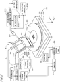
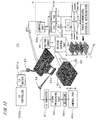
- FIG. 2 shows a configuration of a magnetic field obtaining apparatus 1.
- the magnetic field obtaining apparatus 1 includes a head part 2 that detects interaction between a sample and a sensor in order to control the distance between the sensor and the sample, a sample stage 31 that holds a sample 9 on a horizontal plane, a rotating mechanism 32 for rotating the sample stage 31 about an axis perpendicular to the horizontal plane, a horizontal moving mechanism 33 for moving the sample stage 31 together with the rotating mechanism 32 in the horizontal plane, an elevating mechanism 34 for moving the head part 2 (specifically, a later-described support part 22) in the vertical direction, a signal processing unit 5 for processing signals from the head part 2, and a computer 4 that controls the constituent elements of the magnetic field obtaining apparatus 1 and performs computations.
- a head part 2 that detects interaction between a sample and a sensor in order to control the distance between the sensor and the sample
- a sample stage 31 that holds a sample 9 on a horizontal plane
- a rotating mechanism 32 for rotating the sample stage 31 about an
- the head part 2 includes the measuring part 21 serving as a thin-film element and the support part 22 that holds the measuring part 21.
- the support part 22 has a support plate 221 whose normal line is horizontal, and the measuring part 21 is provided on a lower portion of the support plate 221 in the vertical direction (on the sample 9 side).
- the upper end of the support plate 221 is connected to one side of a sloping part 222 that is a substantially rectangular frame.
- the sloping part 222 is inclined with respect to the horizontal plane and the one side opposite to the support plate 221 is connected to a base part 223 that spreads in the horizontal direction.
- the measuring part 21 is a sensor using a magnetoresistive effect (e.g., giant magnetoresistive (GMR) element) and is formed by laminating a plurality of rectangular films that are long in the horizontal direction on the support plate 221. Output signals from the measuring part 21 are input to the computer 4 via a preamplifier 54 and a signal processing part 55 of the signal processing unit 5. In the measuring part 21, a magnetic field that acts on the entire measuring part 21 is obtained by detection of a change in electrical resistance that occurs due to the magnetic field.
- GMR giant magnetoresistive
- the head part 2 further includes a laser diode module (hereinafter referred to as an "LD module”) 23 and a position sensitive photo-diode (hereinafter referred to as a "PSPD”) 24.
- the LD module 23 is connected to a high-frequency superimposition device 231, and the high-frequency superimposition device 231 is connected to an RF oscillator 232 and an LD bias controller 233.
- the LD module 23 is also connected to an LD temperature controller 234, so that the temperature of the LD module 23 is adjusted to a constant temperature.
- the magnetic field obtaining apparatus 1 Under the control of the computer 4 serving as a control part, light is emitted from the LD module 23 serving as an emission part toward the vicinity of the end portion of the sloping part 222 on the support plate 221 side, and reflected light from the support part 22 is received by the PSPD 24 serving as a light receiving part. Signals from the PSPD 24 are output to the computer 4 via an I-V converter 51, a preamplifier 52, and a signal processing part 53 of the signal processing unit 5. As a result, the position of the support part 22 in the vertical direction is acquired with high precision. This prevents the support plate 221 from coming into contact with the sample 9.
- the horizontal moving mechanism 33 includes first and second moving mechanisms 331 and 332 for horizontally moving the sample stage 31 in two directions perpendicular to each other.
- the directions in which the first and second moving mechanisms 331 and 332 move the sample stage 31 are fixed relative to the measuring part 21.
- the first moving mechanism 331 horizontally moves the sample stage 31 in a direction perpendicular to the longitudinal direction of the measuring part 21, and the second moving mechanism 332 horizontally moves the sample stage 31 in the longitudinal direction.
- the rotating mechanism 32, the horizontal moving mechanism 33, and the elevating mechanism 34 are connected to a driving control part 30.
- the computer 4 is, as shown in Fig. 3 , a general computer system in which a CPU 41 that performs various types of computations, a ROM 42 that stores a basic program, and a RAM 43 that stores various types of information are connected to a bus line.
- a fixed disk 44 that stores information
- a display 45 that displays various types of information
- a keyboard 46a and a mouse 46b that receive input from an operator
- a reading device 47 that reads information from a computer-readable recording medium 8 such as an optical disk, a magnetic disk, or a magneto-optical disk
- a communication part 48 that transmits control signals to the head part 2 and the driving control part 30 and receives input of signals from the signal processing parts 53 and 55.
- a program 441 is read in advance from the recording medium 8 via the reading device 47 and stored in the fixed disk 44.
- the program 441 is then copied into the RAM 43, and the CPU 41 executes computational processing in accordance with the program in the RAM 43 (i.e., the computer 4 executes the program). This realizes a function of a later-described computing part.
- Fig. 4 is a block diagram showing, together with the signal processing unit 5, a functional configuration realized by the CPU 41, the ROM 42, the RAM 43, the fixed disk 44, and the like as a result of the CPU 41 operating in accordance with the program 441.
- Fig. 4 shows functions of a computing part 61 realized by the CPU 41 and the like, and the computing part 61 includes Fourier transforming parts 611 and 612, two-dimensional potential distribution calculating parts 613 and 614, and a three-dimensional potential distribution calculating part 615. Note that these functions may be realized by a dedicated electric circuit, or a dedicated electric circuit may be used in part. Alternatively, these functions may be realized by a plurality of computers.
- Fig. 5 is a flowchart of processing for obtaining a two-dimensional potential (distribution), performed by the magnetic field obtaining apparatus 1.
- the XYZ rectangular coordinate system according to the above-described two-dimensional potential obtaining principle is set fixed relative to the sample 9, the X and Y directions are both horizontal, and the Z direction is vertical.
- the surface of the sample 9 is parallel to the XY plane, and the rotating mechanism 32 rotates the sample stage 31 about the Z axis. Accordingly, when the sample 9 is rotated together with the sample stage 31 by the rotating mechanism 32, the X and Y directions are also rotated together with the sample 9 on the horizontal plane.
- the direction in which the sample stage 31 is moved by the first moving mechanism 331 i.e., horizontal direction perpendicular to the longitudinal direction of the measuring part 21
- the direction in which the sample stage 31 is moved by the second moving mechanism 332 i.e., horizontal direction along the longitudinal direction of the measuring part 21
- a magnetic field specifically, Z-directional component
- the rotating mechanism 32 serving as an angle changing part rotates the sample stage 31, whereby the X and Y directions fixed relative to the sample 9 are rotated together with the sample 9.
- the angle ⁇ formed by the reference direction parallel to the Y direction on the measurement plane and the longitudinal direction of the measuring part 21 (Y' direction) is changed by a fixed small angle (e.g., an angle of 1 degree or more and 15 degrees or less (preferably, 10 degrees or less, and more preferably, 5 degrees or less)) (step S13).
- the measuring part 21 is moved in the X' direction relative to the sample 9 on the measurement plane (i.e., scanning of the measuring part 21 is performed), and a magnetic field is obtained at each position x' (step S11).
- scanning of the measuring part 21 is repeated while the rotating mechanism 32 changes the angle ⁇ to a plurality of angles, as a result of which measured values f(x', ⁇ ) using x' and ⁇ as parameters are acquired (steps S12, S13, and S11).
- the plurality of angles ⁇ in the present embodiment are equidistant angles in a range of greater than or equal to 0° and less than 180°.
- the Fourier transforming part 611 Fourier transforms the measured values f(x', ⁇ ) with respect to x' so as to obtain g(k x' , ⁇ ). Then, the two-dimensional potential distribution calculating part 613 substitutes g(k x' , ⁇ ) into the two-dimensional potential obtaining equation (Equation 10) so as to obtain ⁇ (x, y, ⁇ ) that indicates a two-dimensional potential on the measurement plane (step S14).
- the measuring part 21 that is sufficiently longer than the width of the measurement target area is used, and scanning in the direction perpendicular to the longitudinal direction of the measuring part 21 is repeated on the measurement plane while changing the angle ⁇ formed by the reference direction on the measurement plane and the longitudinal direction of the measuring part 21 to a plurality of angles. Then, the measured values f(x', ⁇ ) obtained by repetitions of the scanning are used to obtain ⁇ (x, y, ⁇ ) that indicates a two-dimensional potential on the measurement plane by the two-dimensional potential obtaining equation.
- the measuring part 21 that is sufficiently larger than the width of the measurement target area, it is possible to perform two-dimensional potential measurement with a high resolution (e.g., nanoscale resolution) in both the X and Y directions.
- the resolution is determined by the film thickness of the thin-film element. Since it is easy to control the thickness of a thin film, in principle the resolution can be improved to the atomic or molecular scale.
- a superconducting quantum interference device having a long measurement range in the horizontal direction may be used as the measuring part 21 (the same applies to apparatuses described below).
- a three-dimensional potential is obtained using a technique similar to that of WO/2008/123432 (Document 2). With the technique described below, ⁇ (x, y, z) indicating a three-dimensional potential that satisfies the Laplace equation is obtained.
- Equation 12 The general solution of this equation can be represented by Equation 12 as the sum of a term that exponentially decreases in the Z direction in the XYZ rectangular coordinate system and a term that exponentially increases in the Z direction in the system.
- ⁇ x y z ⁇ exp ik x x + ik y y a k x k y exp z k x 2 + k y 2 + b k x k y exp ⁇ z k x 2 + k y 2 dk x dk y
- Equation 12 k x and k y are respectively wavenumbers in the X direction and the Y direction, and a(k x , k y ) and b(k x , k y ) are functions represented by k x and k y . Both sides of Equation 12 are further differentiated once with respect to z, the result of which is represented by Equation 13.
- ⁇ z x y z ⁇ exp ik x x + ik y y k x 2 + k y 2 a k x k y exp z k x 2 + k y 2 ⁇ b k x k y exp ⁇ z k x 2 + k y 2 dk x dk y
- Equation 14 ⁇ exp ik x x + ik y y a k x k y + b k x k y dk x dk y
- Equation 16 ⁇ (k x , k y )
- z 0 and ⁇ z (k x , k y )
- z 0 (hereinafter simply expressed as ⁇ (k x , k y ), ⁇ z (k x , k y )) obtained by Fourier transforming ⁇ (x, y, 0) and ⁇ z (x, y, 0) are respectively represented by Equations 16 and 17.
- Equations 16 and 17 it is possible to obtain a(k x , k y ) and b(k x , k y ) that are respectively represented by Equations 18 and 19.
- a k x k y 1 2 ⁇ k x k y + ⁇ z k x k y k x 2 + k y 2
- b k x k y 1 2 ⁇ k x k y ⁇ ⁇ z k x k y k x 2 + k y 2
- Equation 20 ⁇ exp ik x x + ik y y 1 2 ⁇ k x k y + ⁇ z k x k y k x 2 + k y 2 exp z k x 2 + k y 2 + 1 2 ⁇ k x k y ⁇ ⁇ z k x k y k x 2 + k y 2 exp ⁇ z k x 2 + k y 2 + ⁇ z k x 2 + k y 2 + ⁇ z k x 2 + k y 2 + ⁇ z k x 2 + k y 2 + ⁇ z k x 2 + k y 2 + dk x dk y
- H z (q) (x, y, z) and H z (p) (x, y, z) represent functions that are obtained by differentiating a field function H(x, y, z) q times and p times, respectively, with respect to z, the field function H (x, y, z) indicating a field that satisfies the Laplace equation.
- Equation 21 h z (q) (k x , k y ) represents a Fourier transformed function of H z (q) (x, y, 0) (i.e., Equation 21) with respect to x and y
- h z (p) (k x , k y ) represents a Fourier transformed function of H z (p) (x, y, 0) with respect to x and y
- H z (q) (x, y, z) and H z (p) (x, y, z) are respectively represented by Equations 22 and 23.
- H z q x y 0 ⁇ q H z x y z ⁇ z q
- H z (q) (x, y, 0) and H z (p) (x, y, 0) are Fourier transformed so as to obtain h (q) (k x , k y ) and h (p) (k x , k y ) and derive a Fourier transformed function of H z (q) (x, y, z) or H z (p) (x, y, z) from h (q) (k x , k y ) and h (p) (k x , k y ) using Equation 22 or 23, and it is inverse-Fourier transformed, whereby it is possible to obtain H z (q) (x, y, z) or H z (p) (x, y, z).
- the magnetic field obtaining apparatus 1 in Fig. 2 is also capable of obtaining a three-dimensional potential using the above-described three-dimensional potential obtaining method.
- Fig. 6 is a flowchart of processing for obtaining a three-dimensional potential, performed by the magnetic field obtaining apparatus 1.
- the two-dimensional potential distribution calculating part 613 converts a value of ⁇ (x, y, 0) (value indicating the magnitude of a magnetic field) at each position on the measurement plane 91 into a pixel value, and a two-dimensional distribution of the magnetic field on the measurement plane 91 is stored as a magnetic field distribution image 71 (to be precise, image data) in the fixed disk 44 (see Fig. 4 ) ( Fig. 6 : step S21).
- the processing of step S21 has already been completed by execution of the previously-described processing in Fig. 5 .
- the head part 2 is moved down by a small distance d (d > 0) in the Z direction by the elevating mechanism 34 shown in Fig. 2 , so that the distance between the measuring part 21 and the sample 9 is changed by the small distance d as indicated by the dashed double-dotted line in Fig. 7 . That is, a plane 92 that is away from the measurement plane 91 fixed relative to the sample 9 by the small distance d in the (-Z) direction is taken as a new measurement plane. Then, steps S11 to S14 in Fig.
- step S22 a magnetic field distribution on the measurement plane 92 (i.e., ⁇ (x, y, -d)) is obtained as an auxiliary magnetic field distribution image 72 (step S22).
- the measured values f(x', ⁇ ) are output from the signal processing unit 5 to the Fourier transforming part 612 in Fig. 4 , and the two-dimensional potential distribution calculating part 614 generates the auxiliary magnetic field distribution image 72.
- both of the magnetic field distribution image 71 and the auxiliary magnetic field distribution image 72 may be generated by a single Fourier transforming part and a single two-dimensional potential distribution calculating part.
- the three-dimensional potential distribution calculating part 615 obtains a difference image between these two images and divides the difference image by the small distance d so as to generate a differential image.
- the differential image is an image that substantially indicates a Z-directional differentiation of the magnetic field on the measurement plane 91, i.e., the gradient of the magnetic field, and is stored as a magnetic field gradient distribution image (which can also be taken as a potential gradient distribution image) (step S23).
- the magnetic field distribution image 71 is expressed as ⁇ (x, y, 0). Since the gradient of the magnetic field is obtained by differentiating the magnetic field with respect to z, the magnetic field gradient distribution image is an image that indicates ⁇ z (1) (x, y, 0) (hereinafter expressed as ⁇ z (x, y, 0)). If the magnetic field distribution image 71 is a first image, the auxiliary magnetic field distribution image 72 is an intermediate image, and the magnetic field gradient distribution image is a second image, steps S21 to S23 are steps of obtaining the two-dimensional first and intermediate images that indicate the magnetic field distribution and then obtaining the second image that indicates the gradient of the magnetic field from the first and intermediate images.
- the three-dimensional potential distribution calculating part 615 Fourier transforms the magnetic field distribution image 71 expressed as ⁇ (x, y, 0) and the magnetic field gradient distribution image expressed as ⁇ z (x, y, 0) with respect to x and y so as to obtain ⁇ (k x , k y ) and ⁇ z (k x , k y ) (where k x and k y are respectively wavenumbers in the X direction and the Y direction) (step S24).
- a two-dimensional discrete Fourier transform is performed as a Fourier transform, and for example, a technique in which both of the images are multiplied by the n-th power (n is 0 or greater) of a sine function in the range of 0 to ⁇ as a window function is employed for Fourier transforms.
- Equation 20 (hereinafter referred to as a "three-dimensional potential obtaining equation") using ⁇ (k x , k y ) and ⁇ z (k x , k y ) (step S25).
- the three-dimensional potential distribution calculating part 615 substitutes a value (-h) that indicates the position of the measurement target material surface 93 that is embedded in the medium (or value that indicates a position close to the measurement target material surface 93 that is embedded in the medium) into z of ⁇ (x, y, z) so as to obtain a magnetic field distribution on the measurement target material surface 93 that is embedded in the medium (step S26).
- the magnetic field obtaining apparatus 1 Since the magnetic domain structure on the measurement target material surface 93 that is embedded in the medium corresponds to the magnetic field distribution, the magnetic field obtaining apparatus 1 stores an image indicating ⁇ (x, y, -h) as a magnetic domain image that indicates the magnetic domain structure in the fixed disk 44.
- the magnetic field obtaining apparatus 1 realizes a magnetic field microscope having a high spatial resolution of 10 nm or less (or 2 to 3 nm or less depending on the design).
- the magnetic field distribution image 71 and the auxiliary magnetic field distribution image 72 on two different measurement planes that are away from each other by a small distance in the Z direction are obtained using similar techniques, and a difference image between these images is divided by the small distance so as to obtain a differential image as a magnetic field gradient distribution image.
- ⁇ (x, y, 0) that indicates the magnetic field distribution image 71 and ⁇ z (x, y, 0) that indicates the magnetic field gradient distribution image are respectively Fourier transformed so as to obtain ⁇ (k x , k y ) and ⁇ z (k x , k y ), and ⁇ (x, y, z) is obtained from the three-dimensional potential obtaining equation using ⁇ (k x , k y ) and ⁇ z (k x , k y ).
- a three-dimensional potential can be obtained with high precision.
- the computing part 61 substituting a value that indicates either the position of the measurement target material surface 93 of the sample 9 that is embedded in the medium or a position close to the measurement target material surface 93 that is embedded in the medium into z of ⁇ (x, y, z), it is possible to obtain a magnetic domain image that indicates a magnetic domain structure on the measurement target material surface 93 that is embedded in the medium.
- the magnetic field obtaining apparatus 1 can thus realize a magnetic field microscope having a high spatial resolution.
- the magnetic field obtaining apparatus 1 are capable of measuring magnetic domains embedded in a non-magnetic substance even if the surface of the sample 9 is not clean, and is thus applicable as a practical evaluation apparatus or an inspection apparatus used on the manufacturing line. It is also conceivable to use the magnetic field obtaining apparatus 1 as a detector used in a hard disk driving apparatus.
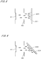
- Fig. 8 shows a condition in which a thin film of a magnetic material is formed on a rectangular substrate (hereinafter denoted by the same reference numeral 221) that will serve as the support plate 221 of the support part 22.
- the measuring part 21 is a multilayer film of a magnetic material (material including cobalt (Co), nickel (Ni), iron (Fe) or the like).
- the substrate 221 is disposed in parallel with a plate-like evaporation source 81 at a position opposed to the evaporation source 81 for the magnetic material, and a mask 82 having an opening is disposed between the evaporation source 81 and the substrate 221 (In Fig. 8 , parallel oblique lines that indicate a cross section are not shown, and the same applies to Fig. 9 ). Then, a thin film 220 of the magnetic material is formed on an area of the substrate 221 that corresponds to the shape of the opening of the mask 82 by vacuum deposition.
- a thin film element that spreads along the main surface of the substrate 221 i.e., the measuring part 21 that spreads in the Y' and Z directions in Fig. 2 ) is formed by deposition of a substance for forming a thin film.
- Fig. 9 shows a condition in which a thin film of a magnetic material is formed on a substrate 221.
- the substrate 221 is disposed so as to face a plate-like evaporation source 81 and to be inclined with respect to the evaporation source 81.
- the lower side in Fig. 9 corresponds to the (-Z) side in the magnetic field obtaining apparatus 1 of Fig. 2 , and the rectangular substrate 221 is inclined such that the lower portion of the substrate 221 is away from the evaporation source 81.
- a thin film 220 is formed in the lower portion of the substrate 221 so as to have a film thickness that gradually decreases toward the lower side.
- a measuring part is formed such that the film thickness of the thin film 220 on the lower side of the substrate 221 (i.e., the sample 9 side in the magnetic field obtaining apparatus 1) is smaller than that of the other portion.
- the measuring part since the resolution in the X' direction serving as the film thickness direction is affected by the film thickness of the lower end portion of the thin film 220 (in actuality, the film thickness of the multilayer film), the measuring part that is formed using the technique shown in Fig.
- Such that the film thickness gradually decreases toward the object is capable of obtaining a measured value having a high resolution in the X' direction as compared with the measuring part formed using the technique shown in Fig. 8 .
- Such a thin film element whose film thickness gradually decreases toward the object may be formed using another technique.
- Fig. 10 is a diagram illustrating an inspection apparatus 1a that employs the above-described two-dimensional potential obtaining method.
- the inspection apparatus 1a is an MRI apparatus that obtains an image through magnetic resonance imaging (MRI).
- the left side in Fig. 10 shows a configuration of the inspection apparatus 1a, and the right side shows the relationship between the Z-directional position of a cross section of an object 9a to be inspected (which is a cross section parallel to the XY plane in Fig. 10 and hereinafter referred to as an "inspection target surface") and the frequency ⁇ of a rotating magnetic field that is applied to the object 9a by a transmission coil 12 described later.
- MRI magnetic resonance imaging
- the inspection apparatus 1a includes a static magnetic field forming part 11 that forms a gradient magnetic field in the Z direction with respect to the object 9a that is a human body lying in the Y direction in Fig. 10 , the transmission coil 12 that applies a rotating magnetic field to the object 9a, a head part 2a disposed on the (+Z) side of the object 9a, a rotating mechanism 32a for rotating the head part 2a around an axis parallel to the Z direction, an elevating mechanism 34a for elevating the head part 2a in the Z direction together with the rotating mechanism 32a, a horizontal moving mechanism 33a for moving the head part 2a in the X and Y directions together with the rotating mechanism 32a and the elevating mechanism 34a, and a control unit 40 that is connected to the constituent elements of the inspection apparatus 1a.
- the head part 2a includes a measuring part 21a that is sufficiently (e.g., two or more times) longer than the width of the object 9a in the X direction, and a support plate 221a to which the measuring part 21a is fixed.
- the support plate 221a is attached to the rotating mechanism 32a via a support bar 224.
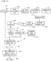
- Fig. 11 shows a functional configuration of the control unit 40 together with the measuring part 21a and the transmission coil 12.
- a control part 62 and a computing part 63 in Fig. 11 are functions realized by a computer included in the control unit 40.
- the control part 62 is connected to a scanning signal generator 410, and the head part 2a is moved by the horizontal moving mechanism 33a so as to perform scanning based on a signal from the scanning signal generator 410.
- the control part 62 is also connected to the transmission coil 12 via an oscillator 401, a phase adjustment part 402, an amplitude modulator 403, and a high-frequency amplifier 404, and a rotating magnetic field of frequency according to control of the control part 62 is applied from the transmission coil 12 to the object 9a.
- the measuring part 21a is connected to a receiver preamplifier 405, and a signal from the measuring part 21a is amplified by the receiver preamplifier 405 and is output to a phase detector 406, an LPF 407, and an A-D converter 408 in the order. Then, output signals from the A-D converter 408 are stored as measured values f(x', ⁇ ) in a memory 409. Note that in Fig. 11 , the content of each signal output from the A-D converter 408 is indicated by being enclosed in the broken-line rectangle denoted by reference character B1 (the same applies to rectangles B2 and B3).
- a three-dimensional magnetic field reconfiguration part 632 has a function similar to that of the three-dimensional potential distribution calculating part 615 in Fig. 4 , and obtains ⁇ (x, y, z) based on ⁇ (x, y, ⁇ ), as well as an MRI image described later.
- a rotating magnetic field with a frequency ⁇ 0 also called an RF pulse (90-degree pulse)
- NMR nuclear magnetic resonance
- an MRI image on the inspection target surface is obtained by the measuring part 21a performing scanning in synchronization with the application of a rotating magnetic field.
- the measuring part 21a is stopped at each position x' in the scanning direction (i.e., X' direction). Then, a rotating magnetic field with the frequency ⁇ 0 is applied from the transmission coil 12 to the object 9a, which induces nuclear magnetic resonance on the inspection target surface.
- a change in the measured value obtained by the measuring part 21a is obtained for a predetermined amount of time after driving of the transmission coil 12 has stopped (i.e., after the application of the rotating magnetic field has stopped).
- Driving the transmission coil 12 and obtaining a change in the measured value after driving of the transmission coil 12 has stopped is performed at all positions x' in the X' direction during the scan. This completes a single scan by the measuring part 21a.
- a magnetic field distribution image expressed as ⁇ (x, y, 0) is obtained by the reconfiguration control part 631 ( Fig. 5 : step S14, Fig. 6 : step S21).
- ⁇ (x, y, 0, t) that includes elapsed time t that has elapsed after the driving of the transmission coil 12 had stopped, as a parameter, is obtained as a function that indicates a magnetic field distribution image for each elapsed time t.
- step S21 processing similar to the above-described processing of step S21 is performed so as to obtain ⁇ (x, y, -d, t) as a function that indicates an auxiliary magnetic field distribution image for each elapsed time t (step S22).
- ⁇ (x, y, 0, t) and ⁇ (x, y, -d, t) is divided by the small distance d so as to obtain ⁇ z (x, y, 0, t) (i.e., magnetic field gradient distribution image obtained by dividing a difference image between the magnetic field distribution image and the auxiliary magnetic field distribution image for each elapsed time t by the small distance d) (step S23).
- ⁇ (x, y, 0, t) and ⁇ z (x, y, 0, t) are respectively Fourier transformed and used to obtain ⁇ (x, y, z, t) by the three-dimensional potential obtaining equation (steps S24 and S25).
- ⁇ (x, y, z, t) indicates ⁇ (x, y, z) for each elapsed time t after driving of the transmission coil 12 has stopped. Accordingly, by substituting z0 into z of ⁇ (x, y, z, t) obtained for the inspection target surface, ⁇ (x, y, z0, t) that indicates a temporal change in the magnetic field at each position (x, y) on the inspection target surface after the application of the rotating magnetic field has stopped is obtained as a function that indicates an excited-state relaxation phenomenon. Then, through predetermined computation, an image that indicates a difference in the relaxation phenomenon at each position (x, y) on the inspection target surface is obtained as an MRI image (step S26).
- steps S21 to S26 are repeated while using each of a plurality of planes located at a plurality of positions in the Z direction as the inspection target surface.
- a rotating magnetic field with a frequency ( ⁇ 0 - ⁇ ) is applied to the object 9a.
- y is the gyromagnetic ratio
- Gz is the gradient of a gradient magnetic field
- MRI images on a plurality of planes located at a plurality of positions in the Z direction are obtained.
- the static magnetic field forming part 11 and the transmission coil 12 operate cooperatively and thereby nuclear magnetic resonance is sequentially induced inside the object 9a on a plurality of planes located at a plurality of positions in the Z direction. Then, when nuclear magnetic resonance has been induced on each plane included in the plurality of planes, the control part 62 causes the computing part 63 to obtain ⁇ (x, y, z) for each elapsed time t and further causes the computing part 63 to substitute a value that indicates the position of the plane into z of ⁇ (x, y, z). As a result, a relaxation phenomenon is obtained at each position (x, y) on the plane serving as the inspection target surface.
- the inspection apparatus 1a enables high-precision inspection using nuclear magnetic resonance.
- the inspection apparatus 1a in Fig. 10 is also capable of reducing senses of oppression and closeness that a subject may feel toward a general tunnel-type MRI apparatus. Since, unlike a normal MRI, the inspection apparatus 1a does not need to form a steep gradient of the magnetic field in the X and Y directions, the spatial resolution in the X and Y directions is determined by the film thickness of the thin-film magnetic field sensor, which enables high-resolution inspection. This makes it possible to realize downsizing of the apparatus and enables clinical application such as real-time high-resolution inspection during a surgical operation.
- the measuring part 21 or 21a obtains a measured value based on a potential derived by differentiating a magnetic potential once with respect to the Z direction
- the measuring part may obtain a measured value based on a potential that is derived by differentiating a magnetic potential twice with respect to the Z direction.
- ⁇ (x, y, z) is ⁇ z (2) (x, y, z) (hereinafter expressed as ⁇ zz (x, y, z)) that is obtained by differentiating ⁇ (x, y, z) twice with respect to z.
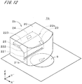
- Fig. 12 shows part of a magnetic field obtaining apparatus 1b according to a second embodiment of the present invention.
- the magnetic field obtaining apparatus 1b differs from the magnetic field obtaining apparatus 1 in Fig. 2 in the configuration of a head part 2b.
- the other constituent elements are similar to those in Fig. 2 and thus not shown in Fig. 12 .
- a thin film that is formed of a magnetic material and is magnetized is provided as a measuring part 21b on a support plate 221 of a support part 22b, and a magnetic force acts between the entire measuring part 21b that is long in the Y' direction and a sample 9.
- the support plate 221 is connected to a base part 223 via a sloping part 222, and the base part 223 is provided with a vibrating part 25 that causes a cantilevered support part 22b (hereinafter referred to as a "cantilever 22b") to vibrate.
- the head part 2b is provided with an LD module 23 and a PSPD 24 that are similar to those of the head part 2 in Fig.
- the measuring part 21b, the cantilever 22b, the vibrating part 25, the LD module 23, and the PSPD 24 are housed in a closed container 20.
- the inside of the container 20 is decompressed so as to improve the Q-value of the cantilever 22b.
- the side faces and upper face ((+Z)-side face) of the container 20 are made of a predetermined magnetic shielding material and enable a considerable reduction in the influence of noise during measurement in connection with the improvement in the Q-value of the cantilever 22b.
- the cantilever 22b is excited up and down at a resonant frequency with piezoelectricity of the vibrating part 25.
- the cantilever 22b is irradiated with light from the LD module 23, and the position of reflected light is detected by the PSPD 24.
- the signal processing part 53 detects the amount of shift of the resonant frequency of the cantilever 22b caused by interaction with the sample 9.
- the shift amount of the frequency at which the cantilever vibrates is derived from interaction and can be said as a measurement amount derived from a conservative force gradient.
- a value that indicates a magnetic force gradient is obtained at each position in the X' direction, based on the shift amount of the resonant frequency of the cantilever 22b.
- ⁇ (x, y, ⁇ ) that indicates a magnetic field gradient distribution image is obtained using a technique similar to that used in the magnetic field obtaining apparatus 1 in Fig. 2 .
- a magnetic field gradient distribution image is obtained as an intermediate image on a measurement plane that is away from the former measurement plane by a small distance (step S22).
- a difference image between the first image and the intermediate image is divided by the small distance d so as to obtain a differential image that indicates a differential in the magnetic field gradient with respect to z, as a second image (step S23).
- a value that indicates the position of the surface of the sample 9 is substituted into z of ⁇ (x, y, z) so as to obtain a magnetic field gradient distribution on the surface, based on which a magnetic domain image is generated (step S26).
- the magnetic field obtaining apparatus 1b measured values f(x', ⁇ ) based on a potential derived by differentiating a magnetic potential twice with respect to the Z direction are obtained by the measuring part 21b, which realizes generation of ⁇ (x, y, z) that is ⁇ zz (x, y, z).
- the magnetic field obtaining apparatus 1b may also be configured such that a measuring part capable of obtaining a measured value based on a potential derived by differentiating a magnetic potential three or more times with respect to the Z direction is provided, and a potential that is derived by differentiating the magnetic potential three or more times with respect to the Z direction is obtained as ⁇ (x, y, z).
- a potential that is derived by differentiating a magnetic potential once or more times with respect to the Z direction is obtained as ⁇ (x, y, z), and a value that indicates either the position of the surface of the sample 9, which is an object, or a position close to that surface is substituted into z of ⁇ (x, y, z). Accordingly, it is possible to realize a high-resolution magnetic field microscope.
- the magnetic field obtaining apparatus 1b in Fig. 12 may be configured such that the amount of displacement of the cantilever 22b is obtained by the LD module 23 and the PSPD 24 while the cantilever 22b that is not caused to vibrate performs scanning, so that the measuring part 21b obtains measured values f(x', ⁇ ) based on a potential derived by differentiating a magnetic potential once with respect to the Z direction and thereby obtains ⁇ (x, y, z) that is ⁇ z (x, y, z) (the same applies to an MRI apparatus described later).
- ⁇ zz (x, y, 0) and ⁇ zzz (x, y, 0) can be obtained by measurement
- ⁇ (x, y, ⁇ ) obtained by another measurement is H z (p) (x, y, 0) that is obtained by differentiating the potential H(x, y, z) p times with respect to z (where p and q are integers greater than or equal to 0, q being odd and p being even)
- H z (q) (x, y, 0) and H z (p) (x, y, 0) are respectively Fourier transformed so as to obtain h z (q) (k x , k y ) and h z (p) (k x , k y ) (where k x
- the magnetic field obtaining apparatus 1b in Fig. 12 may be used as an MRI apparatus.
- the static magnetic field forming part 11 and transmission coil 12 in Fig. 10 are additionally provided in the magnetic field obtaining apparatus 1b, so that nuclear magnetic resonance is sequentially induced inside an object on a plurality of planes located at a plurality of positions in the Z direction.
- such a magnetic field obtaining apparatus may be provided with a measuring part that is capable of obtaining a measured value based on a potential derived by differentiating a magnetic potential three or more times with respect to the Z direction, and may obtain a potential derived by differentiating a magnetic potential three or more times with respect to the Z direction, as ⁇ (x, y, z, t).
- the magnetic field obtaining apparatus realizes high-precision inspection using nuclear magnetic resonance as a result of obtaining a potential that is derived by differentiating a magnetic potential once or more times with respect to the Z direction, as ⁇ (x, y, z).
- a three-dimensional potential (i.e., ⁇ (x, y, z) obtained using the three-dimensional potential obtaining equation) that provides a basis for a two-dimensional potential ⁇ (x, y, ⁇ ) obtained using the two-dimensional potential obtaining equation is not limited to a potential derived from a magnetic potential, and may be a three-dimensional potential distribution of a potential derived from an electric potential that is easy to apply the two-dimensional potential obtaining method.
- the sample 9 is assumed to have electric charge on its surface.
- a measuring part 21b where its surface is covered with an insulator and the insulator holds electric charge is prepared.
- the amount of displacement of the cantilever 22b is obtained as a measured value by the LD module 23 and the PSPD 24 while the cantilever 22b that is not caused to vibrate performs scanning.
- ⁇ (x, y, ⁇ ) that indicates a two-dimensional potential distribution, i.e., an electrostatic force distribution image that indicates the distribution of (the Z-directional component of) an electrostatic force due to the presence of the sample 9, is obtained.
- ⁇ (x, y, z) that indicates a three-dimensional potential distribution (where ⁇ (x, y, z) satisfies the Laplace equation)
- a difference between two electrostatic force distribution images on measurement planes whose positions are different from each other by a small distance in the Z direction is divided by the small distance so as to obtain an electrostatic force gradient distribution image
- a value of z that indicates the position of the surface of the sample 9 (or a position close to the surface) is substituted into the reproduced potential function so as to obtain an image that indicates the distribution of the electrostatic force on the surface of the sample 9 as an image corresponding to the distribution of electric charge.
- a potential distribution that precisely reflects a three-dimensional distribution of electric charge can be obtained from a position that is sufficiently away from the sample 9, without being affected by short range interaction. For example, when electric charge is distributed in three dimensions in an insulating film, it is possible to specify a position at which the electric charge is trapped, from a field that is formed far away by the electric charge.
- the electrostatic force gradient distribution image may be obtained as ⁇ (x, y, ⁇ ) from the shift amount of the oscillation frequency of the resonating cantilever 22b.
- ⁇ (x, y, z) that indicates a three-dimensional distribution of the electrostatic force gradient may be derived based on two electrostatic force gradient distribution images on measurement planes whose positions are different from each other by a small distance in the Z direction.
- the above-described two- and three-dimensional potential obtaining methods are applicable to an arbitrary three-dimensional potential formed at least in the periphery of an object due to the presence of the object, and can also be applied to, besides the potentials derived from magnetic and electric potentials, potentials derived from temperature, and the like.
- a measuring part capable of measuring an average temperature in a measurement range that is long in one direction (the temperature being considered to be equivalent to an integrated value of temperatures in that measurement range) is disposed in the vicinity of an object. Then, the steady-state flow of heat is induced in the object, and scanning with the measuring part is repeated while changing an angle ⁇ formed by a reference direction on a measurement plane and the longitudinal direction of the measuring part to a plurality of angles.
- ⁇ (x, y, ⁇ ) that indicates a temperature distribution on the measurement plane can be obtained. It is also possible, by obtaining temperature distributions on two measurement planes whose positions are diffrent from each other by a small distance in the Z direction, to obtain a three-dimensional temperature distribution ⁇ (x, y, z) in an object and thereby know the internal structure of the object.
- Fig. 13 shows one example of a three-dimensional temperature distribution obtaining apparatus 1c capable of performing such measurement.
- the temperature distribution obtaining apparatus 1c in Fig. 13 includes a measuring part 21c having a thin-film thermocouple.
- the thin-film thermocouple is formed by, for example, sequentially laminating platinum (Pt) and constantan on a substrate.
- a signal from the measuring part 21c is input via an amplifier to a computer 4 similar to that in the apparatus shown in Fig. 2 .
- the computer 4 is shown by a broken-line rectangle, and functions realized by the computer 4 are shown in that rectangle.
- An object 9c to be measured is placed on a sample stage 31 that is rotatable and movable by a rotating mechanism 32 and a horizontal moving mechanism 33. Note that the object 9c is connected to a voltage source 90, and therefore, the steady-state flow of heat is induced in the object 9c.
- the measuring part 21c is movable in the Z direction by an elevating mechanism not shown, and an output from the measuring part 21c is input via a control part 62a to converting parts 610a and 610b.
- converting parts 610a and 610b two-dimensional temperature distributions are obtained at two positions in the Z direction in the same manner as in the apparatus shown in Fig. 2 .
- a three-dimensional temperature distribution (three-dimensional potential distribution) ⁇ (x, y, z) in the object 9c is obtained based on the two two-dimensional temperature distributions. Note that, like the apparatus in Fig.
- the temperature distribution obtaining apparatus 1c is provided with an LD module 23 and a PSPD 24, and laser light is emitted from the LD module 23 by an LD controller 233a driving an LD driver 231a.
- An output from the PSPD 24 is input to the control part 62a via an IV converter 51, a signal processing part 53, and a selector 541 (although in Fig. 13 , for convenience of illustration, this control part 62a is shown as a different block from the one connected to the measuring part 21c, both of the blocks indicate the same control part 62a). This prevents the measuring part 21c from coming into contact with the object 9c.
- a measurement unit that obtains measured values f(x', ⁇ ) is realized by a measuring part, a rotating mechanism, a horizontal moving mechanism, and a computer (or a control part), the measurement unit may be realized by other configurations.
- Fig. 14 is a bottom view of an element group 210 provided in another measurement unit. As shown in Fig. 14 , in the element group 210 in which a large number of thin film elements 21d, each serving as a sensor that extends in the longitudinal direction, are laminated in the film thickness direction, measured values at respective positions in the X' direction at one angle ⁇ are obtained at the same time. Then, the measurement with the element group 210 is repeated while rotating the element group 210 or an object about the Z axis and thereby changing the angle ⁇ to a plurality of angles, so as to obtain the measured values f(x', ⁇ ).
- the element group 210 is configured to simultaneously obtain measured values in a plurality of linear areas that are arranged in the X' direction perpendicular to the longitudinal direction and parallel to the measurement plane. Furthermore, in the measurement unit of the above-described embodiments in which the measuring part performs scanning, the operation of scanning performed by the measuring part that is long in the longitudinal direction is equivalent to setting a plurality of linear areas such that the linear areas are arranged in the X' direction at one angle ⁇ and then obtaining a measured value in each of the plurality of linear areas.
- the potential obtaining apparatus for obtaining ⁇ (x, y, ⁇ ) can realize, in various forms, the measurement unit in which a plurality of linear areas that extend in the longitudinal direction parallel to a measurement plane are set such that the linear areas are arranged in the X' direction perpendicular to the longitudinal direction on the measurement plane, and that is for obtaining a measured value in each of the plurality of linear areas in a state in which the angle ⁇ formed by the reference direction and the longitudinal direction is changed to a plurality of angles.
- the magnetic field obtaining apparatus 1 in Fig. 2 (as well as the other apparatuses) obtains the magnetic field distribution image 71 and the auxiliary magnetic field distribution image 72 at two positions that are away from each other by a small distance d in the Z direction, if the width (height) of the measuring part 21 in the Z direction is sufficiently greater than the small distance d, measurement may be performed by, for example, sequentially disposing the bottom face of the measuring part 21 at three heights z1, z2, and z3 in the Z direction as shown in Fig. 15 .
- a difference image between the z1 image ⁇ (x, y, z1) and the z2 image ⁇ (x, y, z2) is treated as a magnetic field distribution image
- a difference image between the z2 image ⁇ (x, y, z2) and the z3 image ⁇ (x, y, z3) is treated as an auxiliary magnetic field distribution image.
- this technique it is important to make sure that a magnetic field formed due to the presence of the sample 9 is substantially 0 in a portion of the measuring part 21 that is farthest from the sample 9.
- this technique may be adopted in the X' direction perpendicular to both the longitudinal direction and the Z direction.
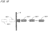
- the sample 9 e.g., sample of a ferromagnetic or ferrimagnetic material
- a limited range can be magnetized (a magnetically oriented area is prevented from spreading in a wide range), and preferable measurement is possible.
- the directivity of a magnetic field at the time of magnetization may be further increased by providing, besides the plurality of coils 901 provided on one main surface side, a plurality of similar coils 901 on the other main surface side as indicated by dashed double-dotted line rectangles in Fig. 16 .
- the speed of measuring a three-dimensional potential may be increased by aligning the support part 22 in Fig. 2 and the cantilever 22b in Fig. 12 in the scanning direction so that the magnetic field distribution image and the magnetic field gradient distribution image are obtained substantially at the same time.
- Two- and three-dimensional potentials do not necessarily have to be obtained in strict accordance with the above-described two- and three-dimensional potential obtaining equations, and may be obtained as appropriate through similar, approximate, or modified computations. It is also possible to employ various well-known skillful techniques for Fourier and inverse-Fourier transforms.
- the measuring parts 21 and 21a to 21c by forming the measuring parts 21 and 21a to 21c as thin-film elements that spread in the Y' direction and the Z direction, it is possible to improve the resolution of measurement in the scanning direction during scanning with the measuring parts 21 and 21a to 21c and to further improve the resolution of measuring a two-dimensional potential.
- Configurations are possible in which the measuring part 21 in the magnetic field obtaining apparatus 1 in Fig. 2 is rotated around the Z axis, and the member for supporting the object 9a in the inspection apparatus 1a in Fig. 10 is rotated around the Z axis. Configurations are also possible in which the measuring part 21 in Fig. 2 is moved on a measurement plane, and the member for supporting the object 9a in Fig. 10 is moved in the horizontal direction together with the object 9a. In this way, it is sufficient for the rotation and movement of the measuring part on a measurement plane to be relative to an object.
- the measuring parts 21, 21a, and 21b are moved in the Z direction by the elevating mechanisms 34 and 34a, it is sufficient for the movement of the measuring part in the Z direction to be relative to an object.
- An elevating mechanism for moving an object in the Z direction may be provided as a Z-directional moving mechanism.
Description
- The present invention relates to a technique for obtaining a two-dimensional potential distribution derived from a magnetic potential, an electric potential, temperature, or the like by measurement.
- Conventionally, the distribution of a magnetic field has been obtained using a superconducting quantum interference device (hereinafter referred to as an "SQUID") or a magnetoresistive sensor, and for example, a defective (or short-circuited) portion of an electric circuit has been specified based on the magnetic field distribution. Since the resolution of the magnetic field measurement depends on the size of the SQUID coil or the magnetoresistive sensor, attempts are being made to reduce that size in order to improve the resolution of the measurement.
- Obtaining the spatial distribution of a magnetic field has also been performed using magnetic force microscopy (hereinafter referred to as "MFM"). Japanese translation of
PCT International Application Publication No. 2006-501484 -
WO/2008/123432 (Document 2) discloses a technique for obtaining a three-dimensional potential distribution. With this technique, a magnetic force distribution on a specific measurement plane is obtained as a two-dimensional magnetic field distribution image, using an MFM above a sample having magnetic domains. An auxiliary magnetic field distribution image is also obtained by performing measurement on another measurement plane that is away from the above measurement plane by a small distance d, and a difference between these images is divided by the small distance d so as to obtain a two-dimensional magnetic field gradient distribution image. The magnetic field distribution image and the magnetic field gradient distribution image are Fourier transformed and substituted into a three-dimensional potential distribution obtaining equation derived from the general solution of the Laplace equation. It is thus possible to obtain an image that indicates a three-dimensional magnetic field distribution with high precision. - Incidentally, there is a limit to miniaturization of the SQUID coil or the magnetoresistive sensor because of the wavelength used in exposure technology, and thus there is also a certain limit to improvement in the resolution of the measurement. Moreover, although the radius of curvature of the tip of a silicon probe formed by anisotropic etching can be reduced to an extremely small value as small as several nanometers, it is necessary, when using the silicon probe in an MFM, to form a thin film of a magnetic material on the tip of the probe. This makes a magnetic force sensor that has a thickness equal to the "film thickness of the magnetic thin film + radius of curvature of the tip of the probe + the magnetic thin film". For example, if the film thickness of the magnetic thin film is 10 nm and the radius of curvature of the tip of the probe is 10 nm, the magnetic force sensor has a total diameter of 30 nm. At least there are no cases where the resolution of the measurement exceeds the radius of curvature of the tip of the probe. In addition, since it is difficult in practical use to cover only the tip portion of the probe with the magnetic thin film, the size of the effective magnetic force sensor is further increased.
-
JP 2007 271465 A - The problem of the present application is therefore related to improving the resolution of universal two-dimensional potential measurements and calculating the three-dimensional potentials formed at least in the periphery of an object.
- This problem is solved by the independent claims. Preferred embodiments are given by the dependent claims.
- An object of the present invention is to improve the resolution of measurement of a two-dimensional potential (two-dimensional potential distribution) derived from a magnetic potential, an electric potential, temperature field, or the like. This object is achieved with a potential obtaining apparatus and a method in accordance with
claims 1 and 7, respectively. - The present invention is intended for a potential obtaining apparatus for, assuming that ϕ(x, y, z) is a potential function that indicates a three-dimensional potential formed at least in the periphery of an object due to the presence of the object (where x, y, and z are coordinate parameters of a rectangular coordinate system defined in mutually perpendicular X, Y, and Z directions that are set for the object), obtaining ϕ(x, y, α) on a measurement plane that is set outside the object and satisfies z = α (where α is an arbitrary value). The apparatus includes a measurement unit in which a plurality of linear areas that extend in a longitudinal direction parallel to the measurement plane that is parallel to an XY plane are set so as to be arranged in an X' direction perpendicular to the longitudinal direction on the measurement plane, and that is for obtaining a measured value derived from the three-dimensional potential in each of the plurality of linear areas in a state in which an angle θ formed by the Y direction and the longitudinal direction has been changed to a plurality of angles, and a computing part for, assuming that x' is a coordinate parameter in the X' direction (where an origin is on a Z axis), obtaining ϕ(x, y, α) from
Equation 1 using the measured values f(x', θ) obtained by the measurement unit,
- According to the present invention, the measurement unit includes a measuring part that extends in the longitudinal direction and is for obtaining a measured value derived from the three-dimensional potential, an angle changing part for changing the angle θ formed by the reference direction and the longitudinal direction of the measuring part, a moving mechanism for moving the measuring part in the X' direction relative to the object on the measurement plane such that scanning is performed in which the measuring part passes through over a measurement area of the object, and a control part for controlling the angle changing part and the moving mechanism such that the scanning is repeated while the angle θ is changed to a plurality of angles. The measurement unit obtains measured values f(x', θ) by repetitions of the scanning.
- Preferably, the three-dimensional potential is a potential derived by differentiating a magnetic potential once or more times with respect to the Z direction, and the measuring part is a thin-film element that spreads in the longitudinal direction and the Z direction and generates a signal derived from the three-dimensional potential. In this case, the resolution of measurement in the scanning direction during scanning with the measuring part can be improved.
- According to the present invention, the potential obtaining apparatus further includes another moving mechanism for moving the measuring part in the Z direction relative to the object. The three-dimensional potential satisfies the Laplace equation. The control part obtains ϕ(x, y, 0) on the measurement plane that satisfies z = 0 as a two-dimensional first image, and after the measuring part is moved by a small distance in the Z direction relative to the object, obtains a two-dimensional intermediate image using a technique similar to that used to obtain the first image. The computing part obtains a difference image between the first image and the intermediate image, divides the difference image by the small distance so as to obtain a differential image as a second image, Fourier transforms ϕ(x, y, 0) serving as the first image and ϕz(x, y, 0) serving as the second image so as to obtain ψ(kx, ky) and ψz(kx, ky) (where kx and ky are respectively wavenumbers in the X direction and the Y direction), and then obtains ϕ(x, y, z) from
Equation 2 using ψ(kx, ky) and ψz(kx, ky).
- It is preferable for the three-dimensional potential to be a potential derived from a magnetic potential, an electric potential, or a temperature field.
- The present invention is also intended for a magnetic field microscope using the potential obtaining apparatus described above and for an inspection apparatus using nuclear magnetic resonance. The prevent invention is also intended for a potential obtaining method.
- These and other objects, features, aspects and advantages of the present invention will become more apparent from the following detailed description of the present invention when taken in conjunction with the accompanying drawings.
-
-
Fig. 1 is a diagram illustrating the principle of a two-dimensional potential obtaining method; -
Fig. 2 shows a configuration of a magnetic field obtaining apparatus; -
Fig. 3 shows a configuration of a computer; -
Fig. 4 is a block diagram showing a functional configuration realized by the computer; -
Fig. 5 is a flowchart of processing for acquiring a two-dimensional potential; -
Fig. 6 is a flowchart of processing for acquiring a three-dimensional potential; -
Fig. 7 shows a measuring part and a measurement plane; -
Fig. 8 shows a condition in which a thin film of a magnetic material is formed on a substrate; -
Fig. 9 shows a condition in which a thin film of a magnetic material is formed on a substrate; -
Fig. 10 is a diagram illustrating an inspection apparatus; -
Fig. 11 shows a functional configuration of a control unit; -
Fig. 12 shows part of a magnetic field obtaining apparatus according to a second embodiment; -
Fig. 13 shows a configuration of a temperature distribution obtaining apparatus; -
Fig. 14 is a bottom view of an element group; -
Fig. 15 is a diagram illustrating another example of obtaining a magnetic field distribution image; and -
Fig. 16 is a diagram illustrating magnetization of a sample. - First, the principle of a two-dimensional potential obtaining method according to the present invention will be described.
Fig. 1 is a diagram illustrating the principle of the two-dimensional potential obtaining method. A rectangular coordinate system defined by mutually perpendicular X, Y, and Z directions is shown inFig. 1 . In the following description, coordinate parameters in the X, Y, and Z directions are respectively indicated by x, y, and z. A thin film-like measuring part denoted byreference numeral 21 inFig. 1 extends in a direction parallel to an arbitrary measurement plane (measurement plane parallel to an XY plane) that satisfies z = α (where a is an arbitrary value) on the measurement plane. - In one example of the two-dimensional potential obtaining method according to the present invention, based on the assumption of the presence of a magnetic potential formed at least in the periphery of an object due to the presence of the object, such as a magnetic potential formed by a magnetized magnetic substance in the periphery thereof or a magnetic potential formed by the current flowing inside the semiconductor device in the periphery of (and inside) a multilayer semiconductor device, a two-dimensional potential (potential distribution) on a measurement plane of a three-dimensional potential derived from the magnetic potential is obtained. Specifically, when the measuring
part 21 is configured to obtain a Z-directional component of a magnetic field (which may be a magnetic field substantially along the Z direction and is hereinafter also simply referred to as a "magnetic field"), a two-dimensional potential on a measurement plane of a three-dimensional potential where a Z-directional gradient of the magnetic potential Φ is taken as a scalar value is obtained. That is, if Φ(x, y, z) is a potential function that indicates a magnetic potential and φ (x, y, z) is a potential function that indicates the above three-dimensional potential, φ (x, y, z) is Φz (1)(x, y, z) (hereinafter expressed as Φz(x, y, z)) that is derived by differentiating Φ(x, y, z) once with respect to z, and the two-dimensional potential obtaining method is a method for obtaining φ (x, y, α) on an arbitrary measurement plane that satisfies z = α. - In the following description, it is assumed that a direction parallel to the Y direction on a measurement plane is a reference direction, the longitudinal direction of the measuring
part 21 is a Y' direction, a direction perpendicular to the longitudinal direction (Y' direction) on the measurement plane is X' direction, θ is the angle formed by the reference direction and the Y' direction, and x' and y' are respectively coordinate parameters in the X' direction and the Y' direction (where the origin of the X' and Y' directions is on the Z axis and is the same as the origin of the rectangular coordinate system defined by the X, Y, and Z directions inFig. 1 ). - In the two-dimensional potential obtaining method, scanning is performed such that the measuring
part 21 is moved in the X' direction so as to pass through a predetermined area on the measurement plane (the area that is obtained by projecting an area to be measured on an object onto the measurement plane and that is hereinafter referred to as a "measurement target area"). During the scanning, a signal indicating a magnetic field received by the measuringpart 21 as a whole (a total sum of magnetic lines of force passing through inside the measuring part 21) is generated at each position x' in the X' direction (that is, the measuringpart 21 detects a magnetic field and generates an electric signal corresponding to the magnetic field) and is obtained as a measured value. In actuality, scanning in a direction perpendicular to the longitudinal direction is repeated on the measurement plane while changing the angle θ to a plurality of angles in a range of greater than or equal to 0° and less than 180°. As a result, a function f(x', θ) that indicate measured values (hereinafter simply referred to as "measured values f(x', 0)") derived from the three-dimensional potential are obtained, using x' and θ as parameters. Note that the Z axis passes through substantially the center of the measurement target area. - Here, the X'Y' coordinate system when viewed along the Z direction can be considered as a coordinate system obtained by rotating the XY coordinate system by the angle θ about the Z axis. Thus, the following Equation 3 is satisfied.

- As described previously, during each scan in which the measuring
part 21 is moved in the X' direction, a magnetic field received by the measuringpart 21 as a whole is obtained. Thus, the measured values f(x', θ) are represented byEquation 4. Note that, in relation to the longitudinal direction (Y' direction) of the measuringpart 21, the measuringpart 21 is set so as to have a length that is sufficiently longer than the width of the measurement target area.
- Here, φ (kx, ky)|z=α (hereinafter simply expressed as φ (kx, ky)) obtained by Fourier transforming φ (x, y, α) with respect to the X and Y directions is represented by
Equation 5. InEquation 5, kx and ky are respectively wavenumbers in the X and Y directions.
- Substituting (kx = kx'cosθ), (ky = kx'sinθ), and (x' = xcosθ + ysinθ) into
Equation 5 yields Equation 6. In Equation 6, kx' and ky' are respectively wavenumbers in the X' and Y' directions.
- Also, (dxdy) in Equation 6 is represented by Equation 7.

- Accordingly, Equation 6 can be transformed into
Equation 8 usingEquations 3, 4, and 7. InEquation 8, φ (kx'cosθ, kx'sinθ) is expressed as g(kx', θ).
- Meanwhile, φ (x, y, α) can be represented by
Equation 9, where (kx = kx'cosθ), (ky = kx'sinθ), and (x' = xcosθ + ysinθ).
- By substituting φ (kxcosθ, kx'sinθ) of
Equation 8 intoEquation 9, φ (x, y, α) is represented by Equation 10.
- Consequently, by performing scanning on the measurement plane with the measuring
part 21 so as to obtain measured values f(x', θ) while changing the angle θ formed by the reference direction and the longitudinal direction of the measuringpart 21 to a plurality of angles and then by Fourier transforming the measured values f(x', θ) with respect to x' so as to obtain g(kx', θ), it is possible to obtain φ (x, y, α) using Equation 10 (hereinafter referred to as a "two-dimensional potential obtaining equation"). - Next is a description of a magnetic field obtaining apparatus using the above-described two-dimensional potential obtaining method.
Fig. 2 shows a configuration of a magneticfield obtaining apparatus 1. The magneticfield obtaining apparatus 1 includes ahead part 2 that detects interaction between a sample and a sensor in order to control the distance between the sensor and the sample, asample stage 31 that holds asample 9 on a horizontal plane, arotating mechanism 32 for rotating thesample stage 31 about an axis perpendicular to the horizontal plane, a horizontal movingmechanism 33 for moving thesample stage 31 together with therotating mechanism 32 in the horizontal plane, an elevatingmechanism 34 for moving the head part 2 (specifically, a later-described support part 22) in the vertical direction, asignal processing unit 5 for processing signals from thehead part 2, and acomputer 4 that controls the constituent elements of the magneticfield obtaining apparatus 1 and performs computations. - The
head part 2 includes the measuringpart 21 serving as a thin-film element and thesupport part 22 that holds the measuringpart 21. Thesupport part 22 has asupport plate 221 whose normal line is horizontal, and the measuringpart 21 is provided on a lower portion of thesupport plate 221 in the vertical direction (on thesample 9 side). The upper end of thesupport plate 221 is connected to one side of asloping part 222 that is a substantially rectangular frame. Thesloping part 222 is inclined with respect to the horizontal plane and the one side opposite to thesupport plate 221 is connected to abase part 223 that spreads in the horizontal direction. - The measuring
part 21 is a sensor using a magnetoresistive effect (e.g., giant magnetoresistive (GMR) element) and is formed by laminating a plurality of rectangular films that are long in the horizontal direction on thesupport plate 221. Output signals from the measuringpart 21 are input to thecomputer 4 via apreamplifier 54 and asignal processing part 55 of thesignal processing unit 5. In the measuringpart 21, a magnetic field that acts on the entire measuringpart 21 is obtained by detection of a change in electrical resistance that occurs due to the magnetic field. - The
head part 2 further includes a laser diode module (hereinafter referred to as an "LD module") 23 and a position sensitive photo-diode (hereinafter referred to as a "PSPD") 24. TheLD module 23 is connected to a high-frequency superimposition device 231, and the high-frequency superimposition device 231 is connected to anRF oscillator 232 and anLD bias controller 233. TheLD module 23 is also connected to anLD temperature controller 234, so that the temperature of theLD module 23 is adjusted to a constant temperature. In the magneticfield obtaining apparatus 1, under the control of thecomputer 4 serving as a control part, light is emitted from theLD module 23 serving as an emission part toward the vicinity of the end portion of thesloping part 222 on thesupport plate 221 side, and reflected light from thesupport part 22 is received by thePSPD 24 serving as a light receiving part. Signals from thePSPD 24 are output to thecomputer 4 via anI-V converter 51, apreamplifier 52, and asignal processing part 53 of thesignal processing unit 5. As a result, the position of thesupport part 22 in the vertical direction is acquired with high precision. This prevents thesupport plate 221 from coming into contact with thesample 9. - The
horizontal moving mechanism 33 includes first and second movingmechanisms 331 and 332 for horizontally moving thesample stage 31 in two directions perpendicular to each other. The directions in which the first and second movingmechanisms 331 and 332 move thesample stage 31 are fixed relative to the measuringpart 21. Thefirst moving mechanism 331 horizontally moves thesample stage 31 in a direction perpendicular to the longitudinal direction of the measuringpart 21, and the second moving mechanism 332 horizontally moves thesample stage 31 in the longitudinal direction. Therotating mechanism 32, the horizontal movingmechanism 33, and the elevatingmechanism 34 are connected to a drivingcontrol part 30. - The
computer 4 is, as shown inFig. 3 , a general computer system in which aCPU 41 that performs various types of computations, aROM 42 that stores a basic program, and aRAM 43 that stores various types of information are connected to a bus line. To the bus line are further connected, via an interface (I/F) where appropriate, a fixeddisk 44 that stores information, adisplay 45 that displays various types of information, akeyboard 46a and amouse 46b that receive input from an operator, areading device 47 that reads information from a computer-readable recording medium 8 such as an optical disk, a magnetic disk, or a magneto-optical disk, and acommunication part 48 that transmits control signals to thehead part 2 and the drivingcontrol part 30 and receives input of signals from thesignal processing parts - In the
computer 4, aprogram 441 is read in advance from therecording medium 8 via thereading device 47 and stored in the fixeddisk 44. Theprogram 441 is then copied into theRAM 43, and theCPU 41 executes computational processing in accordance with the program in the RAM 43 (i.e., thecomputer 4 executes the program). This realizes a function of a later-described computing part. -
Fig. 4 is a block diagram showing, together with thesignal processing unit 5, a functional configuration realized by theCPU 41, theROM 42, theRAM 43, the fixeddisk 44, and the like as a result of theCPU 41 operating in accordance with theprogram 441.Fig. 4 shows functions of acomputing part 61 realized by theCPU 41 and the like, and thecomputing part 61 includesFourier transforming parts distribution calculating parts distribution calculating part 615. Note that these functions may be realized by a dedicated electric circuit, or a dedicated electric circuit may be used in part. Alternatively, these functions may be realized by a plurality of computers. -
Fig. 5 is a flowchart of processing for obtaining a two-dimensional potential (distribution), performed by the magneticfield obtaining apparatus 1. In the following description, it is assumed that the XYZ rectangular coordinate system according to the above-described two-dimensional potential obtaining principle is set fixed relative to thesample 9, the X and Y directions are both horizontal, and the Z direction is vertical. The surface of thesample 9 is parallel to the XY plane, and therotating mechanism 32 rotates thesample stage 31 about the Z axis. Accordingly, when thesample 9 is rotated together with thesample stage 31 by the rotatingmechanism 32, the X and Y directions are also rotated together with thesample 9 on the horizontal plane. It is also assumed that the direction in which thesample stage 31 is moved by the first moving mechanism 331 (i.e., horizontal direction perpendicular to the longitudinal direction of the measuring part 21) is an X' direction, and the direction in which thesample stage 31 is moved by the second moving mechanism 332 (i.e., horizontal direction along the longitudinal direction of the measuring part 21) is an Y' direction. - In the measurement performed by the magnetic
field obtaining apparatus 1 shown inFig. 2 , the measuringpart 21 is disposed on an arbitrary measurement plane that is set outside thesample 9 and satisfies z = α, and by the first movingmechanism 331 moving thesample stage 31 in the X' direction inFig. 2 , scanning is performed in which the measuringpart 21 passes through over a measurement area of the sample 9 (step S11). As result, a magnetic field (specifically, Z-directional component) received by the measuringpart 21 as a whole is obtained as a measured value at each position x' in the X direction that is the scanning direction. - When it is confirmed that the next scanning is to be performed (step S12), the rotating
mechanism 32 serving as an angle changing part rotates thesample stage 31, whereby the X and Y directions fixed relative to thesample 9 are rotated together with thesample 9. As a result, the angle θ formed by the reference direction parallel to the Y direction on the measurement plane and the longitudinal direction of the measuring part 21 (Y' direction) is changed by a fixed small angle (e.g., an angle of 1 degree or more and 15 degrees or less (preferably, 10 degrees or less, and more preferably, 5 degrees or less)) (step S13). Then, the measuringpart 21 is moved in the X' direction relative to thesample 9 on the measurement plane (i.e., scanning of the measuringpart 21 is performed), and a magnetic field is obtained at each position x' (step S11). In the magneticfield obtaining apparatus 1, under the control of thecomputer 4, scanning of the measuringpart 21 is repeated while therotating mechanism 32 changes the angle θ to a plurality of angles, as a result of which measured values f(x', θ) using x' and θ as parameters are acquired (steps S12, S13, and S11). The plurality of angles θ in the present embodiment are equidistant angles in a range of greater than or equal to 0° and less than 180°. - When the measured values f(x', θ) have been obtained by repetitions of the scanning with the measuring part 21 (step S12), the
Fourier transforming part 611 Fourier transforms the measured values f(x', θ) with respect to x' so as to obtain g(kx', θ). Then, the two-dimensional potentialdistribution calculating part 613 substitutes g(kx', θ) into the two-dimensional potential obtaining equation (Equation 10) so as to obtain φ (x, y, α) that indicates a two-dimensional potential on the measurement plane (step S14). - Incidentally, when the two-dimensional distribution of a magnetic field is obtained using a superconducting quantum interference device or a magnetoresistive sensor, there is a technical limit to miniaturization of these devices, and thus there is a certain limit to improvement in the resolution of measurement.
- In contrast, in the magnetic
field obtaining apparatus 1 inFig. 2 serving as a potential obtaining apparatus, the measuringpart 21 that is sufficiently longer than the width of the measurement target area is used, and scanning in the direction perpendicular to the longitudinal direction of the measuringpart 21 is repeated on the measurement plane while changing the angle θ formed by the reference direction on the measurement plane and the longitudinal direction of the measuringpart 21 to a plurality of angles. Then, the measured values f(x', θ) obtained by repetitions of the scanning are used to obtain φ (x, y, α) that indicates a two-dimensional potential on the measurement plane by the two-dimensional potential obtaining equation. As a result, by using the measuringpart 21 that is sufficiently larger than the width of the measurement target area, it is possible to perform two-dimensional potential measurement with a high resolution (e.g., nanoscale resolution) in both the X and Y directions. In this case, the resolution is determined by the film thickness of the thin-film element. Since it is easy to control the thickness of a thin film, in principle the resolution can be improved to the atomic or molecular scale. Note that a superconducting quantum interference device having a long measurement range in the horizontal direction may be used as the measuring part 21 (the same applies to apparatuses described below). - Next is a description of a technique for obtaining a three-dimensional potential (distribution) using the above-described two-dimensional potential obtaining method. A three-dimensional potential is obtained using a technique similar to that of
WO/2008/123432 (Document 2). With the technique described below, φ (x, y, z) indicating a three-dimensional potential that satisfies the Laplace equation is obtained. - First, the principle of obtaining a three-dimensional potential will be described. The three-dimensional potential φ (x, y, z) that satisfies the Laplace equation is represented by
Equation 11 using Laplacian Δ.
- The general solution of this equation can be represented by
Equation 12 as the sum of a term that exponentially decreases in the Z direction in the XYZ rectangular coordinate system and a term that exponentially increases in the Z direction in the system.
- In
Equation 12, kx and ky are respectively wavenumbers in the X direction and the Y direction, and a(kx, ky) and b(kx, ky) are functions represented by kx and ky. Both sides ofEquation 12 are further differentiated once with respect to z, the result of which is represented by Equation 13.
- Here, φ (x, y, z) on a plane that is parallel to the XY plane and satisfies z = 0, namely φ (x, y, 0), is represented by Equation 14.

- Similarly, z = 0 is substituted into Equation 13 and thereby φ z(x, y, 0) is represented by Equation 15.

- Accordingly, φ (kx, ky)|z=0 and φ z(kx, ky)|z=0 (hereinafter simply expressed as φ (kx, ky), φ z(kx, ky)) obtained by Fourier transforming φ (x, y, 0) and φ z(x, y, 0) are respectively represented by Equations 16 and 17.


- From Equations 16 and 17, it is possible to obtain a(kx, ky) and b(kx, ky) that are respectively represented by Equations 18 and 19.


- Here, φ (x, y, z) is represented by
Equation 20 by substituting a(kx, ky) and b(kx, ky) of Equations 18 and 19 intoEquation 12.
- Due to the above, in the case where φ (x, y, 0) serving as the Dirichlet boundary condition and φ z(x, y, 0) serving as the Neumann boundary condition can be obtained by measurement performed on a measurement plane that is set outside the object and satisfies z = 0, they are Fourier transformed so as to derive a Fourier transformed function of φ(x, y, z) with respect to x and y as shown in
Equation 20 and it is inverse-Fourier transformed, whereby it is possible to obtain φ(x, y, z) and to precisely derive a three-dimensional potential. - Meanwhile, a(kx, ky) and b(kx, ky) can also be obtained by performing processing compliant with that for deriving
Equation 20 on functions that are obtained by differentiatingEquation 12 odd times and even times, respectively, with respect to z, and it is possible to derive an equation that corresponds toEquation 20 in which φ (x, y, z) are differentiated once or more times. It is assumed here that q and p are integers greater than or equal to 0, q being odd and p being even (i.e., q = 1, p = 0 (mod 2)). Also, Hz (q)(x, y, z) and Hz (p)(x, y, z) represent functions that are obtained by differentiating a field function H(x, y, z) q times and p times, respectively, with respect to z, the field function H (x, y, z) indicating a field that satisfies the Laplace equation. Assuming that hz (q)(kx, ky) represents a Fourier transformed function of Hz (q)(x, y, 0) (i.e., Equation 21) with respect to x and y, and hz (p)(kx, ky) represents a Fourier transformed function of Hz (p)(x, y, 0) with respect to x and y, Hz (q)(x, y, z) and Hz (p)(x, y, z) are respectively represented byEquations 


- Due to the above, in the case where Hz (q)(x, y, 0) and Hz (p)(x, y, 0) can be obtained by measurement, they are Fourier transformed so as to obtain h(q)(kx, ky) and h(p)(kx, ky) and derive a Fourier transformed function of Hz (q)(x, y, z) or Hz (p)(x, y, z) from h(q)(kx, ky) and h(p)(kx, ky) using
Equation - The magnetic
field obtaining apparatus 1 inFig. 2 is also capable of obtaining a three-dimensional potential using the above-described three-dimensional potential obtaining method.Fig. 6 is a flowchart of processing for obtaining a three-dimensional potential, performed by the magneticfield obtaining apparatus 1. - In the three-dimensional potential obtaining processing, the end face of the measuring
part 21 on the (-Z) side is disposed on ameasurement plane 91 that satisfies z = 0 as indicated by the broken line inFig. 7 , and steps S11 to S14 inFig. 5 are performed so as to obtain φ (x, y, 0). In the present embodiment, the two-dimensional potentialdistribution calculating part 613 converts a value of φ (x, y, 0) (value indicating the magnitude of a magnetic field) at each position on themeasurement plane 91 into a pixel value, and a two-dimensional distribution of the magnetic field on themeasurement plane 91 is stored as a magnetic field distribution image 71 (to be precise, image data) in the fixed disk 44 (seeFig. 4 ) (Fig. 6 : step S21). In actuality, the processing of step S21 has already been completed by execution of the previously-described processing inFig. 5 . - Then, the
head part 2 is moved down by a small distance d (d > 0) in the Z direction by the elevatingmechanism 34 shown inFig. 2 , so that the distance between the measuringpart 21 and thesample 9 is changed by the small distance d as indicated by the dashed double-dotted line inFig. 7 . That is, aplane 92 that is away from themeasurement plane 91 fixed relative to thesample 9 by the small distance d in the (-Z) direction is taken as a new measurement plane. Then, steps S11 to S14 inFig. 5 are performed in a similar manner to the processing of step S21, as a result of which a magnetic field distribution on the measurement plane 92 (i.e., φ (x, y, -d)) is obtained as an auxiliary magnetic field distribution image 72 (step S22). Note that in the processing of step S22, the measured values f(x', θ) are output from thesignal processing unit 5 to theFourier transforming part 612 inFig. 4 , and the two-dimensional potentialdistribution calculating part 614 generates the auxiliary magneticfield distribution image 72. Of course, both of the magneticfield distribution image 71 and the auxiliary magneticfield distribution image 72 may be generated by a single Fourier transforming part and a single two-dimensional potential distribution calculating part. - When the magnetic
field distribution image 71 and the auxiliary magnetic field distribution image 72 (they may be respectively taken as a potential distribution image and an auxiliary potential distribution image) are prepared, the three-dimensional potentialdistribution calculating part 615 obtains a difference image between these two images and divides the difference image by the small distance d so as to generate a differential image. The differential image is an image that substantially indicates a Z-directional differentiation of the magnetic field on themeasurement plane 91, i.e., the gradient of the magnetic field, and is stored as a magnetic field gradient distribution image (which can also be taken as a potential gradient distribution image) (step S23). - As described previously, the magnetic
field distribution image 71 is expressed as φ(x, y, 0). Since the gradient of the magnetic field is obtained by differentiating the magnetic field with respect to z, the magnetic field gradient distribution image is an image that indicates φ z (1)(x, y, 0) (hereinafter expressed as φ z(x, y, 0)). If the magneticfield distribution image 71 is a first image, the auxiliary magneticfield distribution image 72 is an intermediate image, and the magnetic field gradient distribution image is a second image, steps S21 to S23 are steps of obtaining the two-dimensional first and intermediate images that indicate the magnetic field distribution and then obtaining the second image that indicates the gradient of the magnetic field from the first and intermediate images. - Then, the three-dimensional potential
distribution calculating part 615 Fourier transforms the magneticfield distribution image 71 expressed as φ (x, y, 0) and the magnetic field gradient distribution image expressed as φ z(x, y, 0) with respect to x and y so as to obtain φ(kx, ky) and φ z(kx, ky) (where kx and ky are respectively wavenumbers in the X direction and the Y direction) (step S24). Specifically, a two-dimensional discrete Fourier transform is performed as a Fourier transform, and for example, a technique in which both of the images are multiplied by the n-th power (n is 0 or greater) of a sine function in the range of 0 to π as a window function is employed for Fourier transforms. - When φ(kx, ky) and φ z(kx, ky) have been obtained, φ(x, y, z) is obtained by the equation expressed as Equation 20 (hereinafter referred to as a "three-dimensional potential obtaining equation") using φ(kx, ky) and φ z(kx, ky) (step S25). Note that when φ(kx, ky) and φ z(kx, ky) are substituted into the three-dimensional potential obtaining equation and an inverse-Fourier transform is performed with respect to kx and ky, a window function similar to that used for Fourier transforms is used. By obtaining φ (x, y, z), it is possible to precisely derive the three-dimensional distribution of the z component of the magnetic field.
- Next, when, as shown in
Fig. 7 , the distance between a measurementtarget material surface 93 of thesample 9 that is embedded in a medium, and themeasurement plane 91 that satisfies z = 0 is h (h > 0), the three-dimensional potentialdistribution calculating part 615 substitutes a value (-h) that indicates the position of the measurementtarget material surface 93 that is embedded in the medium (or value that indicates a position close to the measurementtarget material surface 93 that is embedded in the medium) into z of φ (x, y, z) so as to obtain a magnetic field distribution on the measurementtarget material surface 93 that is embedded in the medium (step S26). Since the magnetic domain structure on the measurementtarget material surface 93 that is embedded in the medium corresponds to the magnetic field distribution, the magneticfield obtaining apparatus 1 stores an image indicating φ (x, y, -h) as a magnetic domain image that indicates the magnetic domain structure in the fixeddisk 44. Through the above-described operations, even if the sensor cannot be brought close to the measurementtarget material surface 93 that is embedded in the medium due to the influence of a substance such as a protective film that is present on the magnetic material, it is possible to obtain a magnetic field distribution image in the vicinity of the measurementtarget material surface 93 that is embedded in the medium. It is thus possible with the magneticfield obtaining apparatus 1 to realize a magnetic field microscope having a high spatial resolution of 10 nm or less (or 2 to 3 nm or less depending on the design). - As described above, in the magnetic
field obtaining apparatus 1, the magneticfield distribution image 71 and the auxiliary magneticfield distribution image 72 on two different measurement planes that are away from each other by a small distance in the Z direction are obtained using similar techniques, and a difference image between these images is divided by the small distance so as to obtain a differential image as a magnetic field gradient distribution image. Then, φ (x, y, 0) that indicates the magneticfield distribution image 71 and φ z(x, y, 0) that indicates the magnetic field gradient distribution image are respectively Fourier transformed so as to obtain φ(kx, ky) and φ z(kx, ky), and φ(x, y, z) is obtained from the three-dimensional potential obtaining equation using φ(kx, ky) and φ z(kx, ky). As a result, a three-dimensional potential can be obtained with high precision. Moreover, by thecomputing part 61 substituting a value that indicates either the position of the measurementtarget material surface 93 of thesample 9 that is embedded in the medium or a position close to the measurementtarget material surface 93 that is embedded in the medium into z of φ (x, y, z), it is possible to obtain a magnetic domain image that indicates a magnetic domain structure on the measurementtarget material surface 93 that is embedded in the medium. The magneticfield obtaining apparatus 1 can thus realize a magnetic field microscope having a high spatial resolution. - Incidentally, other apparatuses (e.g., a scanning tunneling microscope and a scanning electron microscope) that are used to observe the surface of a magnetic material are able to observe only an extremely clean surface of a magnetic material. In contrast, the magnetic
field obtaining apparatus 1 are capable of measuring magnetic domains embedded in a non-magnetic substance even if the surface of thesample 9 is not clean, and is thus applicable as a practical evaluation apparatus or an inspection apparatus used on the manufacturing line. It is also conceivable to use the magneticfield obtaining apparatus 1 as a detector used in a hard disk driving apparatus. - Next is a description of a preferable technique for forming a thin film in connection with the manufacture of the measuring
part 21.Fig. 8 shows a condition in which a thin film of a magnetic material is formed on a rectangular substrate (hereinafter denoted by the same reference numeral 221) that will serve as thesupport plate 221 of thesupport part 22. As described previously, the measuringpart 21 is a multilayer film of a magnetic material (material including cobalt (Co), nickel (Ni), iron (Fe) or the like). For example, when a thin film of a magnetic material is formed, thesubstrate 221 is disposed in parallel with a plate-like evaporation source 81 at a position opposed to theevaporation source 81 for the magnetic material, and amask 82 having an opening is disposed between theevaporation source 81 and the substrate 221 (InFig. 8 , parallel oblique lines that indicate a cross section are not shown, and the same applies toFig. 9 ). Then, athin film 220 of the magnetic material is formed on an area of thesubstrate 221 that corresponds to the shape of the opening of themask 82 by vacuum deposition. In this way, a thin film element that spreads along the main surface of the substrate 221 (i.e., the measuringpart 21 that spreads in the Y' and Z directions inFig. 2 ) is formed by deposition of a substance for forming a thin film. - Next, a more preferable technique for forming a thin film will be described.
Fig. 9 shows a condition in which a thin film of a magnetic material is formed on asubstrate 221. With the thin-film forming technique shown inFig. 9 , thesubstrate 221 is disposed so as to face a plate-like evaporation source 81 and to be inclined with respect to theevaporation source 81. To be more specific, the lower side inFig. 9 corresponds to the (-Z) side in the magneticfield obtaining apparatus 1 ofFig. 2 , and therectangular substrate 221 is inclined such that the lower portion of thesubstrate 221 is away from theevaporation source 81. Then, evaporation is performed in this state, as a result of which, as shown inFig. 9 , athin film 220 is formed in the lower portion of thesubstrate 221 so as to have a film thickness that gradually decreases toward the lower side. In other words, a measuring part is formed such that the film thickness of thethin film 220 on the lower side of the substrate 221 (i.e., thesample 9 side in the magnetic field obtaining apparatus 1) is smaller than that of the other portion. In the measuring part, since the resolution in the X' direction serving as the film thickness direction is affected by the film thickness of the lower end portion of the thin film 220 (in actuality, the film thickness of the multilayer film), the measuring part that is formed using the technique shown inFig. 9 such that the film thickness gradually decreases toward the object is capable of obtaining a measured value having a high resolution in the X' direction as compared with the measuring part formed using the technique shown inFig. 8 . Such a thin film element whose film thickness gradually decreases toward the object may be formed using another technique. -
Fig. 10 is a diagram illustrating an inspection apparatus 1a that employs the above-described two-dimensional potential obtaining method. The inspection apparatus 1a is an MRI apparatus that obtains an image through magnetic resonance imaging (MRI). The left side inFig. 10 shows a configuration of the inspection apparatus 1a, and the right side shows the relationship between the Z-directional position of a cross section of an object 9a to be inspected (which is a cross section parallel to the XY plane inFig. 10 and hereinafter referred to as an "inspection target surface") and the frequency ω of a rotating magnetic field that is applied to the object 9a by atransmission coil 12 described later. - The inspection apparatus 1a includes a static magnetic
field forming part 11 that forms a gradient magnetic field in the Z direction with respect to the object 9a that is a human body lying in the Y direction inFig. 10 , thetransmission coil 12 that applies a rotating magnetic field to the object 9a, a head part 2a disposed on the (+Z) side of the object 9a, arotating mechanism 32a for rotating the head part 2a around an axis parallel to the Z direction, an elevatingmechanism 34a for elevating the head part 2a in the Z direction together with therotating mechanism 32a, ahorizontal moving mechanism 33a for moving the head part 2a in the X and Y directions together with therotating mechanism 32a and the elevatingmechanism 34a, and acontrol unit 40 that is connected to the constituent elements of the inspection apparatus 1a. InFig. 10 , the lengths of a plurality of arrows indicated by reference character A1 gradually increase in the (-Z) direction from the (+Z) side, thereby showing, in an abstract manner, a state in which the intensity of the static magnetic field formed by the static magneticfield forming part 11 gradually increases in the (-Z) direction. - The head part 2a includes a measuring
part 21a that is sufficiently (e.g., two or more times) longer than the width of the object 9a in the X direction, and asupport plate 221a to which the measuringpart 21a is fixed. Thesupport plate 221a is attached to therotating mechanism 32a via asupport bar 224. -
Fig. 11 shows a functional configuration of thecontrol unit 40 together with the measuringpart 21a and thetransmission coil 12. Acontrol part 62 and acomputing part 63 inFig. 11 are functions realized by a computer included in thecontrol unit 40. - The
control part 62 is connected to ascanning signal generator 410, and the head part 2a is moved by thehorizontal moving mechanism 33a so as to perform scanning based on a signal from thescanning signal generator 410. Thecontrol part 62 is also connected to thetransmission coil 12 via anoscillator 401, aphase adjustment part 402, anamplitude modulator 403, and a high-frequency amplifier 404, and a rotating magnetic field of frequency according to control of thecontrol part 62 is applied from thetransmission coil 12 to the object 9a. The measuringpart 21a is connected to areceiver preamplifier 405, and a signal from the measuringpart 21a is amplified by thereceiver preamplifier 405 and is output to aphase detector 406, anLPF 407, and anA-D converter 408 in the order. Then, output signals from theA-D converter 408 are stored as measured values f(x', θ) in amemory 409. Note that inFig. 11 , the content of each signal output from theA-D converter 408 is indicated by being enclosed in the broken-line rectangle denoted by reference character B1 (the same applies to rectangles B2 and B3). - A
reconfiguration control part 631 of thecomputing part 63 inFig. 11 has a function similar to those of theFourier transforming part 611 and the two-dimensional potentialdistribution calculating part 613 inFig. 4 and obtains φ(x, y, α) on a measurement plane on which the measuringpart 21a is disposed and that satisfies z = α, based on the measured values f(x', θ) stored in thememory 409. A three-dimensional magneticfield reconfiguration part 632 has a function similar to that of the three-dimensional potentialdistribution calculating part 615 inFig. 4 , and obtains φ (x, y, z) based on φ(x, y, α), as well as an MRI image described later. - When a plane of the object 9a that satisfies z = z0 is taken as an inspection target surface, as shown in the right side in
Fig. 10 , a rotating magnetic field with a frequency ω0 (also called an RF pulse (90-degree pulse)) is applied to the object 9a so as to induce nuclear magnetic resonance (NMR) on the inspection target surface of the object 9a. Furthermore, as will be described later, an MRI image on the inspection target surface is obtained by the measuringpart 21a performing scanning in synchronization with the application of a rotating magnetic field. The following is a description of the procedure of inspection operations performed by the inspection apparatus 1a in accordance withFig. 6 . - In the inspection apparatus 1a, the end face of the measuring
part 21a on the (-Z) side is disposed on a measurement plane that satisfies z = 0, and the processing of steps S11 to S13 inFig. 5 is performed. At this time, during each scan performed by the measuringpart 21a in step S11, the measuringpart 21a is stopped at each position x' in the scanning direction (i.e., X' direction). Then, a rotating magnetic field with the frequency ω0 is applied from thetransmission coil 12 to the object 9a, which induces nuclear magnetic resonance on the inspection target surface. Then, a change in the measured value obtained by the measuringpart 21a is obtained for a predetermined amount of time after driving of thetransmission coil 12 has stopped (i.e., after the application of the rotating magnetic field has stopped). Driving thetransmission coil 12 and obtaining a change in the measured value after driving of thetransmission coil 12 has stopped is performed at all positions x' in the X' direction during the scan. This completes a single scan by the measuringpart 21a. By performing the above-described operations during every scan at every angle θ, a magnetic field distribution image expressed as φ (x, y, 0) is obtained by the reconfiguration control part 631 (Fig. 5 : step S14,Fig. 6 : step S21). In actuality, φ (x, y, 0, t) that includes elapsed time t that has elapsed after the driving of thetransmission coil 12 had stopped, as a parameter, is obtained as a function that indicates a magnetic field distribution image for each elapsed time t. - When φ (x, y, 0, t) has been obtained, the head part 2a is moved by a small distance d in the Z direction by the elevating
mechanism 34a. Thereafter, processing similar to the above-described processing of step S21 is performed so as to obtain φ (x, y, -d, t) as a function that indicates an auxiliary magnetic field distribution image for each elapsed time t (step S22). Then, a difference between φ (x, y, 0, t) and φ (x, y, -d, t) is divided by the small distance d so as to obtain φ z(x, y, 0, t) (i.e., magnetic field gradient distribution image obtained by dividing a difference image between the magnetic field distribution image and the auxiliary magnetic field distribution image for each elapsed time t by the small distance d) (step S23). Then, φ (x, y, 0, t) and φ z(x, y, 0, t) are respectively Fourier transformed and used to obtain φ (x, y, z, t) by the three-dimensional potential obtaining equation (steps S24 and S25). - Here, if the position in the Z direction on the inspection target surface is z0, φ (x, y, z, t) indicates φ (x, y, z) for each elapsed time t after driving of the
transmission coil 12 has stopped. Accordingly, by substituting z0 into z of φ (x, y, z, t) obtained for the inspection target surface, φ (x, y, z0, t) that indicates a temporal change in the magnetic field at each position (x, y) on the inspection target surface after the application of the rotating magnetic field has stopped is obtained as a function that indicates an excited-state relaxation phenomenon. Then, through predetermined computation, an image that indicates a difference in the relaxation phenomenon at each position (x, y) on the inspection target surface is obtained as an MRI image (step S26). - The above-described processing of steps S21 to S26 is repeated while using each of a plurality of planes located at a plurality of positions in the Z direction as the inspection target surface. In this case, for example, when a plane that satisfies z = (z0 + Δz) is used as the inspection target surface, a rotating magnetic field with a frequency (φ0 - Δω) is applied to the object 9a. If y is the gyromagnetic ratio and Gz is the gradient of a gradient magnetic field, Δω is expressed as (γ•Gz•Δz) (i.e., (Δω = γ•Gz•Δz)). As a result, MRI images on a plurality of planes located at a plurality of positions in the Z direction are obtained.
- As described above, in the inspection apparatus 1a in
Fig. 10 , the static magneticfield forming part 11 and thetransmission coil 12 operate cooperatively and thereby nuclear magnetic resonance is sequentially induced inside the object 9a on a plurality of planes located at a plurality of positions in the Z direction. Then, when nuclear magnetic resonance has been induced on each plane included in the plurality of planes, thecontrol part 62 causes thecomputing part 63 to obtain φ (x, y, z) for each elapsed time t and further causes thecomputing part 63 to substitute a value that indicates the position of the plane into z of φ (x, y, z). As a result, a relaxation phenomenon is obtained at each position (x, y) on the plane serving as the inspection target surface. This makes it possible to obtain a high-precision MRI image on the inspection target surface. In this way, the inspection apparatus 1a enables high-precision inspection using nuclear magnetic resonance. The inspection apparatus 1a inFig. 10 is also capable of reducing senses of oppression and closeness that a subject may feel toward a general tunnel-type MRI apparatus. Since, unlike a normal MRI, the inspection apparatus 1a does not need to form a steep gradient of the magnetic field in the X and Y directions, the spatial resolution in the X and Y directions is determined by the film thickness of the thin-film magnetic field sensor, which enables high-resolution inspection. This makes it possible to realize downsizing of the apparatus and enables clinical application such as real-time high-resolution inspection during a surgical operation. - Although in the above-described embodiments, the measuring
part -
Fig. 12 shows part of a magneticfield obtaining apparatus 1b according to a second embodiment of the present invention. The magneticfield obtaining apparatus 1b differs from the magneticfield obtaining apparatus 1 inFig. 2 in the configuration of ahead part 2b. The other constituent elements are similar to those inFig. 2 and thus not shown inFig. 12 . - In the
head part 2b, a thin film that is formed of a magnetic material and is magnetized is provided as a measuringpart 21b on asupport plate 221 of asupport part 22b, and a magnetic force acts between the entire measuringpart 21b that is long in the Y' direction and asample 9. Thesupport plate 221 is connected to abase part 223 via asloping part 222, and thebase part 223 is provided with a vibratingpart 25 that causes a cantileveredsupport part 22b (hereinafter referred to as a "cantilever 22b") to vibrate. Thehead part 2b is provided with anLD module 23 and aPSPD 24 that are similar to those of thehead part 2 inFig. 2 , and the measuringpart 21b, thecantilever 22b, the vibratingpart 25, theLD module 23, and thePSPD 24 are housed in aclosed container 20. The inside of thecontainer 20 is decompressed so as to improve the Q-value of thecantilever 22b. The side faces and upper face ((+Z)-side face) of thecontainer 20 are made of a predetermined magnetic shielding material and enable a considerable reduction in the influence of noise during measurement in connection with the improvement in the Q-value of thecantilever 22b. - In the magnetic
field obtaining apparatus 1b, thecantilever 22b is excited up and down at a resonant frequency with piezoelectricity of the vibratingpart 25. Thecantilever 22b is irradiated with light from theLD module 23, and the position of reflected light is detected by thePSPD 24. As a result, the signal processing part 53 (seeFig. 2 ) detects the amount of shift of the resonant frequency of thecantilever 22b caused by interaction with thesample 9. Here, the shift amount of the frequency at which the cantilever vibrates is derived from interaction and can be said as a measurement amount derived from a conservative force gradient. Accordingly, in the magneticfield obtaining apparatus 1b, when the measuringpart 21b performs scanning in the X' direction, a value that indicates a magnetic force gradient (magnetic force gradient in the entire measuringpart 21b) is obtained at each position in the X' direction, based on the shift amount of the resonant frequency of thecantilever 22b. Accordingly, measured values f(x', θ) are obtained by repeating scanning in the direction perpendicular to the longitudinal direction of the measuringpart 21b on the measurement plane while changing the angle θ formed by the reference direction on a measurement plane that satisfies z = a and the longitudinal direction (Y' direction) of the measuringpart 21b to a plurality of angles. Also, φ (x, y, α) that indicates a magnetic field gradient distribution image is obtained using a technique similar to that used in the magneticfield obtaining apparatus 1 inFig. 2 . - In the measurement performed by the magnetic
field obtaining apparatus 1b, the shift amount of the oscillation frequency of thecantilever 22b is obtained on the measurement plane that satisfies z = 0, and then a magnetic field gradient distribution image is obtained as a first image (Fig. 6 : step S21). Similarly, a magnetic field gradient distribution image is obtained as an intermediate image on a measurement plane that is away from the former measurement plane by a small distance (step S22). Following this, a difference image between the first image and the intermediate image is divided by the small distance d so as to obtain a differential image that indicates a differential in the magnetic field gradient with respect to z, as a second image (step S23). In this case, since the first image corresponds to φ (x, y, 0) (i.e., Φzz(x, y, 0)) and the second image corresponds to φ z(x, y, 0) (i.e., Φzzz(x, y, 0)), these images are Fourier transformed and substituted into the three-dimensional potential obtaining equation ofEquation 20 so as to obtain φ (x, y, z) that is Φzz(x, y, z) (steps S24 and S25). Then, a value that indicates the position of the surface of thesample 9 is substituted into z of φ (x, y, z) so as to obtain a magnetic field gradient distribution on the surface, based on which a magnetic domain image is generated (step S26). - In this way, in the magnetic
field obtaining apparatus 1b, measured values f(x', θ) based on a potential derived by differentiating a magnetic potential twice with respect to the Z direction are obtained by the measuringpart 21b, which realizes generation of φ (x, y, z) that is Φzz(x, y, z). Of course, the magneticfield obtaining apparatus 1b may also be configured such that a measuring part capable of obtaining a measured value based on a potential derived by differentiating a magnetic potential three or more times with respect to the Z direction is provided, and a potential that is derived by differentiating the magnetic potential three or more times with respect to the Z direction is obtained as φ (x, y, z). - As described above, in the magnetic field obtaining apparatus, a potential that is derived by differentiating a magnetic potential once or more times with respect to the Z direction is obtained as φ (x, y, z), and a value that indicates either the position of the surface of the
sample 9, which is an object, or a position close to that surface is substituted into z of φ (x, y, z). Accordingly, it is possible to realize a high-resolution magnetic field microscope. - Note that the magnetic
field obtaining apparatus 1b inFig. 12 may be configured such that the amount of displacement of thecantilever 22b is obtained by theLD module 23 and thePSPD 24 while thecantilever 22b that is not caused to vibrate performs scanning, so that the measuringpart 21b obtains measured values f(x', θ) based on a potential derived by differentiating a magnetic potential once with respect to the Z direction and thereby obtains φ (x, y, z) that is Φz(x, y, z) (the same applies to an MRI apparatus described later). - The magnetic
field obtaining apparatus 1b may also be configured such that Φz(x, y, 0) is measured by scanning with thecantilever 22b that is not caused to vibrate, Φzz(x, y, 0) is measured by scanning with thecantilever 22b that is caused to vibrate, then Φz(x, y, 0) that is set as Hz (q)(x, y, 0) (where q = 1) and Φzz(x, y, 0) that is set as Hz (p)(x, y, 0) (where p = 2) are Fourier transformed so as to obtain h(q)(kx, ky) and h(p)(kx, ky), and then Hz (p)(x, y, z) (i.e., Φzz(x, y, z)) is obtained usingEquation 23. In the case where Φzz(x, y, 0) and Φzzz(x, y, 0) can be obtained by measurement, a configuration is also possible in which Φzzz(x, y, 0) that is set as Hz (q)(x, y, 0) (where q = 3) and Φzz(x, y, 0) that is set as Hz (p)(x, y, 0) (where p = 2) are Fourier transformed so as to obtain h(q)(kx, ky) and h(p)(kx, ky), and then Hz (q)(x, y, z) (i.e., Φzzz(x, y, z)) is obtained usingEquation 22. - In this way, in the case where φ (x, y, a) obtained by one measurement is Hz (q)(x, y, 0) that is obtained by differentiating an arbitrary potential H(x, y, z) on a measurement plane that satisfies z = 0 q times with respect to z, and φ (x, y, α) obtained by another measurement is Hz (p)(x, y, 0) that is obtained by differentiating the potential H(x, y, z) p times with respect to z (where p and q are integers greater than or equal to 0, q being odd and p being even), Hz (q)(x, y, 0) and Hz (p)(x, y, 0) are respectively Fourier transformed so as to obtain hz (q)(kx, ky) and hz (p)(kx, ky) (where kx and ky are respectively wavenumbers in the X direction and the Y direction). As a result, it is possible to obtain Hz (q)(x, y, z) using
Equation 22 or Hz (p)(x, y, z) using Equation 23 (the same applies to other apparatuses). - The magnetic
field obtaining apparatus 1b inFig. 12 may be used as an MRI apparatus. In this case, the static magneticfield forming part 11 andtransmission coil 12 inFig. 10 are additionally provided in the magneticfield obtaining apparatus 1b, so that nuclear magnetic resonance is sequentially induced inside an object on a plurality of planes located at a plurality of positions in the Z direction. When nuclear magnetic resonance has been induced on each plane included in the plurality of planes, φ (x, y, z, t) that is Φzz(x, y, z, t) is obtained, and a relaxation phenomenon at each position (x, y) on that plane is further obtained by substituting a value that indicates a position of the plane into z of φ (x, y, z, t). As a result, it is possible to obtain a high-precision MRI image on the inspection target surface of the object. - Alternatively, such a magnetic field obtaining apparatus may be provided with a measuring part that is capable of obtaining a measured value based on a potential derived by differentiating a magnetic potential three or more times with respect to the Z direction, and may obtain a potential derived by differentiating a magnetic potential three or more times with respect to the Z direction, as φ (x, y, z, t). As described above, the magnetic field obtaining apparatus realizes high-precision inspection using nuclear magnetic resonance as a result of obtaining a potential that is derived by differentiating a magnetic potential once or more times with respect to the Z direction, as φ (x, y, z).
- A three-dimensional potential (i.e., φ (x, y, z) obtained using the three-dimensional potential obtaining equation) that provides a basis for a two-dimensional potential φ (x, y, α) obtained using the two-dimensional potential obtaining equation is not limited to a potential derived from a magnetic potential, and may be a three-dimensional potential distribution of a potential derived from an electric potential that is easy to apply the two-dimensional potential obtaining method. In this case, for example in the apparatus shown in
Fig. 12 , thesample 9 is assumed to have electric charge on its surface. A measuringpart 21b where its surface is covered with an insulator and the insulator holds electric charge is prepared. Then, at each angle θ, the amount of displacement of thecantilever 22b is obtained as a measured value by theLD module 23 and thePSPD 24 while thecantilever 22b that is not caused to vibrate performs scanning. As a result, φ (x, y, α) that indicates a two-dimensional potential distribution, i.e., an electrostatic force distribution image that indicates the distribution of (the Z-directional component of) an electrostatic force due to the presence of thesample 9, is obtained. - When obtaining φ (x, y, z) that indicates a three-dimensional potential distribution (where φ (x, y, z) satisfies the Laplace equation), a difference between two electrostatic force distribution images on measurement planes whose positions are different from each other by a small distance in the Z direction is divided by the small distance so as to obtain an electrostatic force gradient distribution image, and the electrostatic force distribution image on the measurement plane that satisfies z = 0 and the electrostatic force gradient distribution image are respectively Fourier transformed and substituted into the three-dimensional potential obtaining equation so as to reproduce a three-dimensional potential that indicates an electrostatic force. Furthermore, a value of z that indicates the position of the surface of the sample 9 (or a position close to the surface) is substituted into the reproduced potential function so as to obtain an image that indicates the distribution of the electrostatic force on the surface of the
sample 9 as an image corresponding to the distribution of electric charge. In this way, with the above-described technique, a potential distribution that precisely reflects a three-dimensional distribution of electric charge can be obtained from a position that is sufficiently away from thesample 9, without being affected by short range interaction. For example, when electric charge is distributed in three dimensions in an insulating film, it is possible to specify a position at which the electric charge is trapped, from a field that is formed far away by the electric charge. - Of course, the electrostatic force gradient distribution image may be obtained as φ (x, y, α) from the shift amount of the oscillation frequency of the resonating
cantilever 22b. Alternatively, φ (x, y, z) that indicates a three-dimensional distribution of the electrostatic force gradient may be derived based on two electrostatic force gradient distribution images on measurement planes whose positions are different from each other by a small distance in the Z direction. - The above-described two- and three-dimensional potential obtaining methods are applicable to an arbitrary three-dimensional potential formed at least in the periphery of an object due to the presence of the object, and can also be applied to, besides the potentials derived from magnetic and electric potentials, potentials derived from temperature, and the like. For example, a measuring part capable of measuring an average temperature in a measurement range that is long in one direction (the temperature being considered to be equivalent to an integrated value of temperatures in that measurement range) is disposed in the vicinity of an object. Then, the steady-state flow of heat is induced in the object, and scanning with the measuring part is repeated while changing an angle θ formed by a reference direction on a measurement plane and the longitudinal direction of the measuring part to a plurality of angles. As a result, θ (x, y, α) that indicates a temperature distribution on the measurement plane can be obtained. It is also possible, by obtaining temperature distributions on two measurement planes whose positions are diffrent from each other by a small distance in the Z direction, to obtain a three-dimensional temperature distribution φ (x, y, z) in an object and thereby know the internal structure of the object.
Fig. 13 shows one example of a three-dimensional temperaturedistribution obtaining apparatus 1c capable of performing such measurement. - The temperature
distribution obtaining apparatus 1c inFig. 13 includes a measuringpart 21c having a thin-film thermocouple. The thin-film thermocouple is formed by, for example, sequentially laminating platinum (Pt) and constantan on a substrate. A signal from the measuringpart 21c is input via an amplifier to acomputer 4 similar to that in the apparatus shown inFig. 2 . InFig. 13 , thecomputer 4 is shown by a broken-line rectangle, and functions realized by thecomputer 4 are shown in that rectangle. Anobject 9c to be measured is placed on asample stage 31 that is rotatable and movable by arotating mechanism 32 and a horizontal movingmechanism 33. Note that theobject 9c is connected to avoltage source 90, and therefore, the steady-state flow of heat is induced in theobject 9c. - The measuring
part 21c is movable in the Z direction by an elevating mechanism not shown, and an output from the measuringpart 21c is input via acontrol part 62a to convertingparts 610a and 610b. In the convertingparts 610a and 610b, two-dimensional temperature distributions are obtained at two positions in the Z direction in the same manner as in the apparatus shown inFig. 2 . Then, a three-dimensional temperature distribution (three-dimensional potential distribution) φ (x, y, z) in theobject 9c is obtained based on the two two-dimensional temperature distributions. Note that, like the apparatus inFig. 2 , the temperaturedistribution obtaining apparatus 1c is provided with anLD module 23 and aPSPD 24, and laser light is emitted from theLD module 23 by an LD controller 233a driving anLD driver 231a. An output from thePSPD 24 is input to thecontrol part 62a via anIV converter 51, asignal processing part 53, and a selector 541 (although inFig. 13 , for convenience of illustration, thiscontrol part 62a is shown as a different block from the one connected to the measuringpart 21c, both of the blocks indicate thesame control part 62a). This prevents the measuringpart 21c from coming into contact with theobject 9c. - While the above has been a description of embodiments of the present invention, the present invention is not intended to be limited to the embodiments described above and can be modified in various ways.
- Although in the above-described embodiments, a measurement unit that obtains measured values f(x', θ) is realized by a measuring part, a rotating mechanism, a horizontal moving mechanism, and a computer (or a control part), the measurement unit may be realized by other configurations.
Fig. 14 is a bottom view of anelement group 210 provided in another measurement unit. As shown inFig. 14 , in theelement group 210 in which a large number ofthin film elements 21d, each serving as a sensor that extends in the longitudinal direction, are laminated in the film thickness direction, measured values at respective positions in the X' direction at one angle θ are obtained at the same time. Then, the measurement with theelement group 210 is repeated while rotating theelement group 210 or an object about the Z axis and thereby changing the angle θ to a plurality of angles, so as to obtain the measured values f(x', θ). - Here, if an area of each
thin film element 21d on a measurement plane is taken as a linear area, theelement group 210 is configured to simultaneously obtain measured values in a plurality of linear areas that are arranged in the X' direction perpendicular to the longitudinal direction and parallel to the measurement plane. Furthermore, in the measurement unit of the above-described embodiments in which the measuring part performs scanning, the operation of scanning performed by the measuring part that is long in the longitudinal direction is equivalent to setting a plurality of linear areas such that the linear areas are arranged in the X' direction at one angle θ and then obtaining a measured value in each of the plurality of linear areas. As described above, the potential obtaining apparatus for obtaining φ (x, y, α) can realize, in various forms, the measurement unit in which a plurality of linear areas that extend in the longitudinal direction parallel to a measurement plane are set such that the linear areas are arranged in the X' direction perpendicular to the longitudinal direction on the measurement plane, and that is for obtaining a measured value in each of the plurality of linear areas in a state in which the angle θ formed by the reference direction and the longitudinal direction is changed to a plurality of angles. - When the magnetic
field obtaining apparatus 1 inFig. 2 (as well as the other apparatuses) obtains the magneticfield distribution image 71 and the auxiliary magneticfield distribution image 72 at two positions that are away from each other by a small distance d in the Z direction, if the width (height) of the measuringpart 21 in the Z direction is sufficiently greater than the small distance d, measurement may be performed by, for example, sequentially disposing the bottom face of the measuringpart 21 at three heights z1, z2, and z3 in the Z direction as shown inFig. 15 . In this case, if images obtained at the heights z1, z2, and z3 are respectively referred to as a z1 image φ (x, y, z1), a z2 image φ (x, y, z2), and a z3 image φ (x, y, z3), a difference image between the z1 image φ (x, y, z1) and the z2 image φ (x, y, z2) is treated as a magnetic field distribution image, and a difference image between the z2 image φ (x, y, z2) and the z3 image φ (x, y, z3) is treated as an auxiliary magnetic field distribution image. This makes it possible to obtain a magnetic field distribution image and an auxiliary magnetic field distribution image that are equivalent to those obtained by performing measurement using a measuring part whose width in the Z direction is small, thus allowing a three-dimensional magnetic field distribution to be obtained with high precision. Note that when using this technique, it is important to make sure that a magnetic field formed due to the presence of thesample 9 is substantially 0 in a portion of the measuringpart 21 that is farthest from thesample 9. Alternatively, depending on the design of the measuring part, this technique may be adopted in the X' direction perpendicular to both the longitudinal direction and the Z direction. - When it is necessary, in the measurement of a magnetic field, to magnetize the sample 9 (e.g., sample of a ferromagnetic or ferrimagnetic material) in advance, it is preferable to increase the directivity of a magnetic field at the time of magnetization by arranging a plurality of
coils 901 in a direction perpendicular to thesample 9 as shown inFig. 16 (disposing the coils in multiple stages). As a result, only a limited range can be magnetized (a magnetically oriented area is prevented from spreading in a wide range), and preferable measurement is possible. Note that when a plate-like sample 9 can be magnetized from both main surface sides, the directivity of a magnetic field at the time of magnetization may be further increased by providing, besides the plurality ofcoils 901 provided on one main surface side, a plurality ofsimilar coils 901 on the other main surface side as indicated by dashed double-dotted line rectangles inFig. 16 . - In the magnetic field obtaining apparatus, the speed of measuring a three-dimensional potential may be increased by aligning the
support part 22 inFig. 2 and thecantilever 22b inFig. 12 in the scanning direction so that the magnetic field distribution image and the magnetic field gradient distribution image are obtained substantially at the same time. - Two- and three-dimensional potentials do not necessarily have to be obtained in strict accordance with the above-described two- and three-dimensional potential obtaining equations, and may be obtained as appropriate through similar, approximate, or modified computations. It is also possible to employ various well-known skillful techniques for Fourier and inverse-Fourier transforms.
- In the above-described embodiments, by forming the measuring
parts parts - Configurations are possible in which the measuring
part 21 in the magneticfield obtaining apparatus 1 inFig. 2 is rotated around the Z axis, and the member for supporting the object 9a in the inspection apparatus 1a inFig. 10 is rotated around the Z axis. Configurations are also possible in which the measuringpart 21 inFig. 2 is moved on a measurement plane, and the member for supporting the object 9a inFig. 10 is moved in the horizontal direction together with the object 9a. In this way, it is sufficient for the rotation and movement of the measuring part on a measurement plane to be relative to an object. - Although in the above-described embodiments, the measuring
parts mechanisms - The configurations of the above-described preferred embodiments and variations may be appropriately combined as long as there are no mutual inconsistencies.
- While the invention has been shown and described in detail, the foregoing description is in all aspects illustrative and not restrictive. It is therefore understood that numerous modifications and variations can be devised without departing from the scope of the invention.
-
- 1, 1b
- Magnetic field obtaining apparatus
- 1a
- Inspection apparatus
- 1c
- Temperature distribution obtaining apparatus
- 4
- Computer
- 9
- Sample
- 9a, 9c
- Object
- 11
- Static magnetic field forming part
- 12
- Transmission coil
- 21, 21a to 21c
- Measuring part
- 32, 32a
- Rotating mechanism
- 33, 33a
- Horizontal moving mechanism
- 34, 34a
- Elevating mechanism
- 61, 63
- Computing part
- 62, 62a
- Control part
- 71
- Magnetic field distribution image
- 72
- Auxiliary magnetic field distribution image
- 81
- Evaporation source
- 91, 92
- Measurement plane
- 93
- Surface (of sample)
- 220
- Thin film
- 221
- Substrate
- S11 to S14, S21 to S25
- Step
Claims (9)
- A potential obtaining apparatus (1, 1a to 1c) for, assuming that φ(x, y, z) is a potential function that indicates a three-dimensional potential formed at least in the periphery of an object (9, 9a, 9c) due to the presence of said object, where x, y, and z are coordinate parameters of a rectangular coordinate system defined in mutually perpendicular X, Y, and Z directions that are set for said object, obtaining φ(x, y, α) on a measurement plane (91, 92) that is set outside said object and satisfies z = α, where α is an arbitrary value,
said apparatus comprising:a measurement unit in which a plurality of linear areas that extend in a longitudinal direction parallel to said measurement plane that is parallel to an XY plane are set so as to be arranged in an X' direction perpendicular to said longitudinal direction on said measurement plane, and that is for obtaining, by a sensor extending in said longitudinal direction, a measured value derived from said three-dimensional potential in each of said plurality of linear areas in a state in which an angle θ formed by the Y direction and said longitudinal direction has been changed to a plurality of angles; anda computing part (61, 63) for, assuming that x' is a coordinate parameter in the X' direction, where an origin is on a Z axis, obtaining φ(x, y, α) on the measurement plane (91, 92) using the measured values f(x', θ) obtained by said measurement unit from Equation 24,where kx' is a wavenumber in the X' direction,
wherein said measurement unit includes:a measuring part (21, 21a to 21c) which is said sensor, said measuring part being a thin-film element that spreads in said longitudinal direction and the Z direction and being configured to generate a signal derived from said three-dimensional potential;an angle changing part (32, 32a) for changing said angle θ formed by the Y direction and said longitudinal direction of said measuring part;a moving mechanism (33, 33a) for moving said measuring part in the X' direction relative to said object on said measurement plane such that scanning is performed in which said measuring part is adapted to pass through over a measurement area of said object; anda control part (4, 62, 62a) for controlling said angle changing part and said moving mechanism such that said scanning is repeated while said angle θ is changed to a plurality of angles,wherein said measurement unit is adapted to obtain measured values f(x', θ) by repetitions of said scanning,wherein the potential obtaining apparatus further comprises:another moving mechanism (34, 34a) for moving said measuring part in the Z direction relative to said object,wherein said three-dimensional potential satisfies the Laplace equation,wherein said control part is adapted to obtain φ(x, y, 0) on said measurement plane that satisfies z = 0 as a two-dimensional first image (71), and after said measuring part is moved by a small distance in the Z direction relative to said object, to obtain a two-dimensional intermediate image (72) using a technique similar to that used to obtain said first image, andsaid computing part is adapted to obtain a difference image between said first image and said intermediate image, to divide said difference image by said small distance so as to obtain a differential image as a second image, to Fourier transform φ(x, y, 0) serving as said first image and φ z(x, y, 0) serving as said second image so as to obtain ψ (kx, ky) and ψ z(kx, ky), where kx and ky are respectively wavenumbers in the X direction and the Y direction, and then to obtain φ(x, y, z) from Equation 25 using ψ (kx, ky) and ψz(kx, ky).
- The potential obtaining apparatus according to claim 1, wherein
φ(x, y, z) corresponds to a function derived by differentiating said three-dimensional potential one or more times with respect to the Z direction. - The potential obtaining apparatus according to claim 1, wherein
a film thickness of said thin-film element gradually decreases in a direction along a surface of said thin-film element, the direction being perpendicular to said longitudinal direction. - The potential obtaining apparatus according to any one of claims 1 to 3, wherein
said three-dimensional potential is a potential derived from a magnetic potential, an electric potential, or a temperature field. - A magnetic field microscope (1) comprising:the potential obtaining apparatus according to claim 1 for obtaining a function derived by differentiating a magnetic potential once or more times with respect to the Z direction, as φ(x, y, z),wherein said computing part is adapted to substitute a value that indicates either a position of a surface of said object or a position close to said surface into z of φ(x, y, z).
- An inspection apparatus (1a) using nuclear magnetic resonance, comprising:the potential obtaining apparatus according to claim 1 for obtaining a function derived by differentiating a magnetic potential once or more times with respect to the Z direction, as φ (x, y, z); andmeans (11, 12) for sequentially inducing nuclear magnetic resonance inside said object on a plurality of planes located at a plurality of positions in the Z direction,wherein said control part is adapted to obtain φ(x, y, z) when nuclear magnetic resonance is induced on each plane included in said plurality of planes, andsaid computing part is adapted to substitute a value that indicates a position of said each plane into z of φ (x, y, z) obtained for said each plane.
- A potential obtaining method for, assuming that φ(x, y, z) is a potential function that indicates a three-dimensional potential formed at least in the periphery of an object (9, 9a, 9c) due to the presence of said object, where x, y, and z are coordinate parameters of a rectangular coordinate system defined in mutually perpendicular X, Y, and Z directions that are set for said object, obtaining φ(x, y, α) on a measurement plane (91, 92) that is set outside said object and satisfies z = α, where α is an arbitrary value,
said method comprising the steps of:a) (S11 to S13) setting a plurality of linear areas that extend in a longitudinal direction parallel to said measurement plane that is parallel to an XY plane such that said plurality of linear areas are arranged in an X' direction perpendicular to said longitudinal direction on said measurement plane, and obtaining, by a sensor extending in said longitudinal direction, a measured value derived from said three-dimensional potential in each of said plurality of linear areas in a state in which an angle θ formed by the Y direction and said longitudinal direction has been changed to a plurality of angles; andb) (S14) assuming that x' is a coordinate parameter in the X' direction, where an origin is on a Z axis, obtaining φ(x, y, α) on the measurement plane (91, 92) using the measured values f(x', θ) obtained in said step a) from Equation 26,
wherein said step a) includes the steps of:a1) (S11) moving a measuring part (21, 21a to 21c) in the X' direction relative to said object on said measurement plane such that scanning is performed in which said measuring part is adapted to pass through over a measurement area of said object, said measuring part being said sensor and being a thin-film element that spreads in said longitudinal direction and the Z direction and generates a signal derived from said three-dimensional potential; anda2) (S12 to S13) obtaining measured values f(x', θ) by repetitions of said step a1) while changing said angle θ formed by the Y axis and said longitudinal direction of said measuring part to a plurality of angles,wherein said three-dimensional potential satisfies the Laplace equation and said measurement plane satisfies z = 0,wherein φ(x, y, 0) is obtained as a two-dimensional first image (71) in said steps a) and b), andwherein said potential obtaining method comprises the steps of:c) (S22) after said measuring part is moved by a small distance in the Z direction relative to said object, obtaining a two-dimensional intermediate image (72) using a method similar to that used to obtain said first image;d) (S23) obtaining a difference image between said first image and said intermediate image and dividing said difference image by said small distance so as to obtain a differential image as a second image;e) (S24) Fourier transforming φ(x, y, 0) serving as said first image and φ z(x, y, 0) serving as said second image so as to obtain ψ(kx, ky) and ψ z(kx, ky), where kx and ky are respectively wavenumbers in the X direction and the Y direction; andf) (S25) obtaining φ(x, y, z) from Equation 27 using ψ (kx, ky) and ψ z(kx, ky).
- The potential obtaining method according to claim 7, wherein
φ(x, y, z) corresponds to a function derived by differentiating said three-dimensional potential once or more times with respect to the Z direction. - The potential obtaining method according to any one of claims 7 and 8, wherein
said three-dimensional potential is a potential derived from a magnetic potential, an electric potential, or a temperature field.
Applications Claiming Priority (2)
| Application Number | Priority Date | Filing Date | Title |
|---|---|---|---|
| JP2010044218 | 2010-03-01 | ||
| PCT/JP2011/054635 WO2011108543A1 (en) | 2010-03-01 | 2011-03-01 | Potential obtaining device, magnetic field microscope, inspection device and method of obtaining potential |
Publications (3)
| Publication Number | Publication Date |
|---|---|
| EP2544016A1 EP2544016A1 (en) | 2013-01-09 |
| EP2544016A4 EP2544016A4 (en) | 2015-09-30 |
| EP2544016B1 true EP2544016B1 (en) | 2020-04-15 |
Family
ID=44542193
Family Applications (1)
| Application Number | Title | Priority Date | Filing Date |
|---|---|---|---|
| EP11750653.5A Active EP2544016B1 (en) | 2010-03-01 | 2011-03-01 | Device and method for obtaining a potential |
Country Status (5)
| Country | Link |
|---|---|
| US (1) | US20120330581A1 (en) |
| EP (1) | EP2544016B1 (en) |
| JP (1) | JP5713246B2 (en) |
| KR (1) | KR101346523B1 (en) |
| WO (1) | WO2011108543A1 (en) |
Families Citing this family (6)
| Publication number | Priority date | Publication date | Assignee | Title |
|---|---|---|---|---|
| JP2013120080A (en) * | 2011-12-06 | 2013-06-17 | Murata Mfg Co Ltd | Magnetic field measuring method and device |
| EP2960668B1 (en) * | 2013-02-25 | 2018-05-16 | National University Corporation Kobe University | Distribution analyzing device and distribution analyzing method |
| WO2014197412A1 (en) * | 2013-06-05 | 2014-12-11 | Nanomechanics, Inc. | Electrostatic force tester |
| CN106556750A (en) * | 2016-11-16 | 2017-04-05 | 国网福建省电力有限公司 | Based on three-dimensional electric field measuring method mutually non-coplanar two-by-two |
| JP6291638B1 (en) * | 2016-12-07 | 2018-03-14 | 小野 瑞絵 | Magnetic force measuring device |
| WO2022190753A1 (en) * | 2021-03-09 | 2022-09-15 | 株式会社 Integral Geometry Science | Inspecting device and inspecting method |
Family Cites Families (9)
| Publication number | Priority date | Publication date | Assignee | Title |
|---|---|---|---|---|
| JPH0390877A (en) * | 1989-09-04 | 1991-04-16 | Hitachi Ltd | Instrument and method for measuring distribution of vector physical quantity |
| JPH0493783A (en) * | 1990-08-09 | 1992-03-26 | Fujitsu Ltd | Imaging device of magnetic field |
| JPH0498159A (en) * | 1990-08-17 | 1992-03-30 | Nippon Telegr & Teleph Corp <Ntt> | Method for estimation through visualization of electric field distribution around electric charge |
| JPH09243725A (en) * | 1996-03-06 | 1997-09-19 | Kanazawa Kogyo Univ | Method of measuring magnetic distribution, magnetic distribution measuring device, and magnetic detector plate |
| CA2499370A1 (en) | 2002-09-20 | 2004-06-05 | The Trustees Of Boston College | Nanotube cantilever probes for nanoscale magnetic microscopy |
| WO2005043177A2 (en) * | 2003-10-30 | 2005-05-12 | California Institute Of Technology | Apparatus and method for detection of magnetic resonance by a magneto-resistive sensor |
| JP2007271465A (en) * | 2006-03-31 | 2007-10-18 | Tokyo Institute Of Technology | Magnetic field distribution measuring instrument |
| EP2141481B1 (en) | 2007-03-30 | 2012-05-23 | Kyoto University | Device and method for acquiring a field by measurement |
| JP5435228B2 (en) * | 2007-06-29 | 2014-03-05 | 日本電気株式会社 | Electromagnetic field distribution measuring device |
-
2011
- 2011-03-01 JP JP2012503192A patent/JP5713246B2/en active Active
- 2011-03-01 EP EP11750653.5A patent/EP2544016B1/en active Active
- 2011-03-01 US US13/582,151 patent/US20120330581A1/en not_active Abandoned
- 2011-03-01 KR KR1020127025458A patent/KR101346523B1/en not_active IP Right Cessation
- 2011-03-01 WO PCT/JP2011/054635 patent/WO2011108543A1/en active Application Filing
Non-Patent Citations (1)
| Title |
|---|
| None * |
Also Published As
| Publication number | Publication date |
|---|---|
| JP5713246B2 (en) | 2015-05-07 |
| KR20120125392A (en) | 2012-11-14 |
| EP2544016A1 (en) | 2013-01-09 |
| EP2544016A4 (en) | 2015-09-30 |
| KR101346523B1 (en) | 2013-12-31 |
| JPWO2011108543A1 (en) | 2013-06-27 |
| WO2011108543A1 (en) | 2011-09-09 |
| US20120330581A1 (en) | 2012-12-27 |
Similar Documents
| Publication | Publication Date | Title |
|---|---|---|
| Mamin et al. | Nuclear magnetic resonance imaging with 90-nm resolution | |
| EP2544016B1 (en) | Device and method for obtaining a potential | |
| Rugar et al. | Proton magnetic resonance imaging using a nitrogen–vacancy spin sensor | |
| EP2141481B1 (en) | Device and method for acquiring a field by measurement | |
| CN108181594B (en) | Non-exchange quantum geometric phase magnetometer | |
| US7023204B2 (en) | Magnetic imaging microscope test system and its application for characterization of read and write heads for magnetic recording | |
| US8026715B2 (en) | Magneto-resistance based nano-scale position sensor | |
| Huxter et al. | Scanning gradiometry with a single spin quantum magnetometer | |
| US10539633B2 (en) | Ultrahigh resolution magnetic resonance imaging method and apparatus | |
| Grob et al. | Magnetic resonance force microscopy with a one-dimensional resolution of 0.9 nanometers | |
| Chao et al. | Nanometer-scale magnetic resonance imaging | |
| Tetienne et al. | Quantitative stray field imaging of a magnetic vortex core | |
| US9678186B2 (en) | Probe for magnetic resonance force microscopy and method thereof | |
| US11002812B1 (en) | Nuclear magnetic resonance diffraction | |
| US7042216B2 (en) | Two-dimensional magnetic resonance tomographic microscopy | |
| Nomura et al. | Near-field radio-frequency imaging by spin-locking with a nitrogen-vacancy spin sensor | |
| Toda et al. | Three-dimensional imaging of electron spin resonance-magnetic resonance force microscopy at room temperature | |
| US8170316B2 (en) | Tomographic imaging with a stripe-like shaped sensor | |
| Banuazizi et al. | Magnetic force microscopy of an operational spin nano-oscillator | |
| US6897654B2 (en) | System and method of magnetic resonance imaging | |
| Costa et al. | Integration of magnetoresistive sensors with atomic force microscopy cantilevers for scanning magnetoresistance microscopy applications | |
| US6980004B2 (en) | Apparatus and method for detection of magnetic resonance by a magneto-resistive sensor | |
| JP3566567B2 (en) | Magnetic resonance type exchange interaction force microscope and observation method using the same | |
| Barbic | Magnetic resonance diffraction using the magnetic field from a ferromagnetic sphere | |
| Wijts | Magnetic resonance force microscopy at milliKelvin temperatures |
Legal Events
| Date | Code | Title | Description |
|---|---|---|---|
| PUAI | Public reference made under article 153(3) epc to a published international application that has entered the european phase |
Free format text: ORIGINAL CODE: 0009012 |
|
| 17P | Request for examination filed |
Effective date: 20120927 |
|
| AK | Designated contracting states |
Kind code of ref document: A1 Designated state(s): AL AT BE BG CH CY CZ DE DK EE ES FI FR GB GR HR HU IE IS IT LI LT LU LV MC MK MT NL NO PL PT RO RS SE SI SK SM TR |
|
| DAX | Request for extension of the european patent (deleted) | ||
| RA4 | Supplementary search report drawn up and despatched (corrected) |
Effective date: 20150902 |
|
| RIC1 | Information provided on ipc code assigned before grant |
Ipc: G01N 24/08 20060101ALI20150826BHEP Ipc: G01R 29/14 20060101ALI20150826BHEP Ipc: G01R 33/34 20060101ALI20150826BHEP Ipc: A61B 5/055 20060101ALI20150826BHEP Ipc: G01R 33/38 20060101ALN20150826BHEP Ipc: G01R 33/02 20060101AFI20150826BHEP Ipc: G01R 33/10 20060101ALI20150826BHEP |
|
| STAA | Information on the status of an ep patent application or granted ep patent |
Free format text: STATUS: EXAMINATION IS IN PROGRESS |
|
| RIC1 | Information provided on ipc code assigned before grant |
Ipc: G01R 33/10 20060101ALI20180815BHEP Ipc: G01R 33/38 20060101ALN20180815BHEP Ipc: G01R 33/02 20060101AFI20180815BHEP Ipc: G01N 24/08 20060101ALI20180815BHEP Ipc: A61B 5/055 20060101ALI20180815BHEP Ipc: G01R 29/14 20060101ALI20180815BHEP Ipc: G01R 33/34 20060101ALI20180815BHEP |
|
| 17Q | First examination report despatched |
Effective date: 20180905 |
|
| GRAP | Despatch of communication of intention to grant a patent |
Free format text: ORIGINAL CODE: EPIDOSNIGR1 |
|
| STAA | Information on the status of an ep patent application or granted ep patent |
Free format text: STATUS: GRANT OF PATENT IS INTENDED |
|
| RIC1 | Information provided on ipc code assigned before grant |
Ipc: G01R 33/10 20060101ALI20191009BHEP Ipc: A61B 5/055 20060101ALI20191009BHEP Ipc: G01R 29/14 20060101ALI20191009BHEP Ipc: G01R 33/38 20060101ALN20191009BHEP Ipc: G01N 24/08 20060101ALI20191009BHEP Ipc: G01R 33/34 20060101ALI20191009BHEP Ipc: G01R 33/02 20060101AFI20191009BHEP |
|
| INTG | Intention to grant announced |
Effective date: 20191025 |
|
| GRAS | Grant fee paid |
Free format text: ORIGINAL CODE: EPIDOSNIGR3 |
|
| RAP1 | Party data changed (applicant data changed or rights of an application transferred) |
Owner name: KIMURA, KENJIRO |
|
| RIN1 | Information on inventor provided before grant (corrected) |
Inventor name: KIMURA, KENJIRO |
|
| GRAA | (expected) grant |
Free format text: ORIGINAL CODE: 0009210 |
|
| STAA | Information on the status of an ep patent application or granted ep patent |
Free format text: STATUS: THE PATENT HAS BEEN GRANTED |
|
| AK | Designated contracting states |
Kind code of ref document: B1 Designated state(s): AL AT BE BG CH CY CZ DE DK EE ES FI FR GB GR HR HU IE IS IT LI LT LU LV MC MK MT NL NO PL PT RO RS SE SI SK SM TR |
|
| REG | Reference to a national code |
Ref country code: CH Ref legal event code: EP Ref country code: GB Ref legal event code: FG4D |
|
| REG | Reference to a national code |
Ref country code: DE Ref legal event code: R096 Ref document number: 602011066267 Country of ref document: DE |
|
| REG | Reference to a national code |
Ref country code: IE Ref legal event code: FG4D |
|
| REG | Reference to a national code |
Ref country code: AT Ref legal event code: REF Ref document number: 1257959 Country of ref document: AT Kind code of ref document: T Effective date: 20200515 |
|
| REG | Reference to a national code |
Ref country code: NL Ref legal event code: FP |
|
| REG | Reference to a national code |
Ref country code: LT Ref legal event code: MG4D |
|
| PG25 | Lapsed in a contracting state [announced via postgrant information from national office to epo] |
Ref country code: PT Free format text: LAPSE BECAUSE OF FAILURE TO SUBMIT A TRANSLATION OF THE DESCRIPTION OR TO PAY THE FEE WITHIN THE PRESCRIBED TIME-LIMIT Effective date: 20200817 Ref country code: LT Free format text: LAPSE BECAUSE OF FAILURE TO SUBMIT A TRANSLATION OF THE DESCRIPTION OR TO PAY THE FEE WITHIN THE PRESCRIBED TIME-LIMIT Effective date: 20200415 Ref country code: GR Free format text: LAPSE BECAUSE OF FAILURE TO SUBMIT A TRANSLATION OF THE DESCRIPTION OR TO PAY THE FEE WITHIN THE PRESCRIBED TIME-LIMIT Effective date: 20200716 Ref country code: FI Free format text: LAPSE BECAUSE OF FAILURE TO SUBMIT A TRANSLATION OF THE DESCRIPTION OR TO PAY THE FEE WITHIN THE PRESCRIBED TIME-LIMIT Effective date: 20200415 Ref country code: NO Free format text: LAPSE BECAUSE OF FAILURE TO SUBMIT A TRANSLATION OF THE DESCRIPTION OR TO PAY THE FEE WITHIN THE PRESCRIBED TIME-LIMIT Effective date: 20200715 Ref country code: IS Free format text: LAPSE BECAUSE OF FAILURE TO SUBMIT A TRANSLATION OF THE DESCRIPTION OR TO PAY THE FEE WITHIN THE PRESCRIBED TIME-LIMIT Effective date: 20200815 Ref country code: SE Free format text: LAPSE BECAUSE OF FAILURE TO SUBMIT A TRANSLATION OF THE DESCRIPTION OR TO PAY THE FEE WITHIN THE PRESCRIBED TIME-LIMIT Effective date: 20200415 |
|
| REG | Reference to a national code |
Ref country code: AT Ref legal event code: MK05 Ref document number: 1257959 Country of ref document: AT Kind code of ref document: T Effective date: 20200415 |
|
| PG25 | Lapsed in a contracting state [announced via postgrant information from national office to epo] |
Ref country code: HR Free format text: LAPSE BECAUSE OF FAILURE TO SUBMIT A TRANSLATION OF THE DESCRIPTION OR TO PAY THE FEE WITHIN THE PRESCRIBED TIME-LIMIT Effective date: 20200415 Ref country code: RS Free format text: LAPSE BECAUSE OF FAILURE TO SUBMIT A TRANSLATION OF THE DESCRIPTION OR TO PAY THE FEE WITHIN THE PRESCRIBED TIME-LIMIT Effective date: 20200415 Ref country code: BG Free format text: LAPSE BECAUSE OF FAILURE TO SUBMIT A TRANSLATION OF THE DESCRIPTION OR TO PAY THE FEE WITHIN THE PRESCRIBED TIME-LIMIT Effective date: 20200715 Ref country code: LV Free format text: LAPSE BECAUSE OF FAILURE TO SUBMIT A TRANSLATION OF THE DESCRIPTION OR TO PAY THE FEE WITHIN THE PRESCRIBED TIME-LIMIT Effective date: 20200415 |
|
| PG25 | Lapsed in a contracting state [announced via postgrant information from national office to epo] |
Ref country code: AL Free format text: LAPSE BECAUSE OF FAILURE TO SUBMIT A TRANSLATION OF THE DESCRIPTION OR TO PAY THE FEE WITHIN THE PRESCRIBED TIME-LIMIT Effective date: 20200415 |
|
| REG | Reference to a national code |
Ref country code: DE Ref legal event code: R097 Ref document number: 602011066267 Country of ref document: DE |
|
| PG25 | Lapsed in a contracting state [announced via postgrant information from national office to epo] |
Ref country code: EE Free format text: LAPSE BECAUSE OF FAILURE TO SUBMIT A TRANSLATION OF THE DESCRIPTION OR TO PAY THE FEE WITHIN THE PRESCRIBED TIME-LIMIT Effective date: 20200415 Ref country code: SM Free format text: LAPSE BECAUSE OF FAILURE TO SUBMIT A TRANSLATION OF THE DESCRIPTION OR TO PAY THE FEE WITHIN THE PRESCRIBED TIME-LIMIT Effective date: 20200415 Ref country code: RO Free format text: LAPSE BECAUSE OF FAILURE TO SUBMIT A TRANSLATION OF THE DESCRIPTION OR TO PAY THE FEE WITHIN THE PRESCRIBED TIME-LIMIT Effective date: 20200415 Ref country code: AT Free format text: LAPSE BECAUSE OF FAILURE TO SUBMIT A TRANSLATION OF THE DESCRIPTION OR TO PAY THE FEE WITHIN THE PRESCRIBED TIME-LIMIT Effective date: 20200415 Ref country code: ES Free format text: LAPSE BECAUSE OF FAILURE TO SUBMIT A TRANSLATION OF THE DESCRIPTION OR TO PAY THE FEE WITHIN THE PRESCRIBED TIME-LIMIT Effective date: 20200415 Ref country code: CZ Free format text: LAPSE BECAUSE OF FAILURE TO SUBMIT A TRANSLATION OF THE DESCRIPTION OR TO PAY THE FEE WITHIN THE PRESCRIBED TIME-LIMIT Effective date: 20200415 Ref country code: IT Free format text: LAPSE BECAUSE OF FAILURE TO SUBMIT A TRANSLATION OF THE DESCRIPTION OR TO PAY THE FEE WITHIN THE PRESCRIBED TIME-LIMIT Effective date: 20200415 Ref country code: DK Free format text: LAPSE BECAUSE OF FAILURE TO SUBMIT A TRANSLATION OF THE DESCRIPTION OR TO PAY THE FEE WITHIN THE PRESCRIBED TIME-LIMIT Effective date: 20200415 |
|
| PLBE | No opposition filed within time limit |
Free format text: ORIGINAL CODE: 0009261 |
|
| STAA | Information on the status of an ep patent application or granted ep patent |
Free format text: STATUS: NO OPPOSITION FILED WITHIN TIME LIMIT |
|
| PG25 | Lapsed in a contracting state [announced via postgrant information from national office to epo] |
Ref country code: PL Free format text: LAPSE BECAUSE OF FAILURE TO SUBMIT A TRANSLATION OF THE DESCRIPTION OR TO PAY THE FEE WITHIN THE PRESCRIBED TIME-LIMIT Effective date: 20200415 Ref country code: SK Free format text: LAPSE BECAUSE OF FAILURE TO SUBMIT A TRANSLATION OF THE DESCRIPTION OR TO PAY THE FEE WITHIN THE PRESCRIBED TIME-LIMIT Effective date: 20200415 |
|
| 26N | No opposition filed |
Effective date: 20210118 |
|
| PG25 | Lapsed in a contracting state [announced via postgrant information from national office to epo] |
Ref country code: SI Free format text: LAPSE BECAUSE OF FAILURE TO SUBMIT A TRANSLATION OF THE DESCRIPTION OR TO PAY THE FEE WITHIN THE PRESCRIBED TIME-LIMIT Effective date: 20200415 |
|
| PG25 | Lapsed in a contracting state [announced via postgrant information from national office to epo] |
Ref country code: MC Free format text: LAPSE BECAUSE OF FAILURE TO SUBMIT A TRANSLATION OF THE DESCRIPTION OR TO PAY THE FEE WITHIN THE PRESCRIBED TIME-LIMIT Effective date: 20200415 |
|
| REG | Reference to a national code |
Ref country code: CH Ref legal event code: PL |
|
| GBPC | Gb: european patent ceased through non-payment of renewal fee |
Effective date: 20210301 |
|
| REG | Reference to a national code |
Ref country code: BE Ref legal event code: MM Effective date: 20210331 |
|
| PG25 | Lapsed in a contracting state [announced via postgrant information from national office to epo] |
Ref country code: CH Free format text: LAPSE BECAUSE OF NON-PAYMENT OF DUE FEES Effective date: 20210331 Ref country code: LU Free format text: LAPSE BECAUSE OF NON-PAYMENT OF DUE FEES Effective date: 20210301 Ref country code: LI Free format text: LAPSE BECAUSE OF NON-PAYMENT OF DUE FEES Effective date: 20210331 Ref country code: FR Free format text: LAPSE BECAUSE OF NON-PAYMENT OF DUE FEES Effective date: 20210331 Ref country code: GB Free format text: LAPSE BECAUSE OF NON-PAYMENT OF DUE FEES Effective date: 20210301 Ref country code: IE Free format text: LAPSE BECAUSE OF NON-PAYMENT OF DUE FEES Effective date: 20210301 |
|
| PG25 | Lapsed in a contracting state [announced via postgrant information from national office to epo] |
Ref country code: BE Free format text: LAPSE BECAUSE OF NON-PAYMENT OF DUE FEES Effective date: 20210331 |
|
| PG25 | Lapsed in a contracting state [announced via postgrant information from national office to epo] |
Ref country code: HU Free format text: LAPSE BECAUSE OF FAILURE TO SUBMIT A TRANSLATION OF THE DESCRIPTION OR TO PAY THE FEE WITHIN THE PRESCRIBED TIME-LIMIT; INVALID AB INITIO Effective date: 20110301 Ref country code: CY Free format text: LAPSE BECAUSE OF FAILURE TO SUBMIT A TRANSLATION OF THE DESCRIPTION OR TO PAY THE FEE WITHIN THE PRESCRIBED TIME-LIMIT Effective date: 20200415 |
|
| PGFP | Annual fee paid to national office [announced via postgrant information from national office to epo] |
Ref country code: DE Payment date: 20230317 Year of fee payment: 13 |
|
| PGFP | Annual fee paid to national office [announced via postgrant information from national office to epo] |
Ref country code: NL Payment date: 20230330 Year of fee payment: 13 |
|
| PGFP | Annual fee paid to national office [announced via postgrant information from national office to epo] |
Ref country code: NL Payment date: 20240320 Year of fee payment: 14 |