EP2395375A2 - Extraction of depositional systems - Google Patents
Extraction of depositional systems Download PDFInfo
- Publication number
- EP2395375A2 EP2395375A2 EP11004821A EP11004821A EP2395375A2 EP 2395375 A2 EP2395375 A2 EP 2395375A2 EP 11004821 A EP11004821 A EP 11004821A EP 11004821 A EP11004821 A EP 11004821A EP 2395375 A2 EP2395375 A2 EP 2395375A2
- Authority
- EP
- European Patent Office
- Prior art keywords
- volume
- data
- stratal
- seismic
- slice
- Prior art date
- Legal status (The legal status is an assumption and is not a legal conclusion. Google has not performed a legal analysis and makes no representation as to the accuracy of the status listed.)
- Withdrawn
Links
Images


Classifications
-
- G—PHYSICS
- G01—MEASURING; TESTING
- G01V—GEOPHYSICS; GRAVITATIONAL MEASUREMENTS; DETECTING MASSES OR OBJECTS; TAGS
- G01V1/00—Seismology; Seismic or acoustic prospecting or detecting
- G01V1/28—Processing seismic data, e.g. analysis, for interpretation, for correction
- G01V1/32—Transforming one recording into another or one representation into another
-
- G—PHYSICS
- G01—MEASURING; TESTING
- G01V—GEOPHYSICS; GRAVITATIONAL MEASUREMENTS; DETECTING MASSES OR OBJECTS; TAGS
- G01V1/00—Seismology; Seismic or acoustic prospecting or detecting
- G01V1/28—Processing seismic data, e.g. analysis, for interpretation, for correction
- G01V1/30—Analysis
-
- G—PHYSICS
- G01—MEASURING; TESTING
- G01V—GEOPHYSICS; GRAVITATIONAL MEASUREMENTS; DETECTING MASSES OR OBJECTS; TAGS
- G01V2210/00—Details of seismic processing or analysis
- G01V2210/40—Transforming data representation
- G01V2210/48—Other transforms
Definitions
- An exemplary embodiment of this invention is in the field of 3-D interpretation, and more particularly to 3-D seismic interpretation. More specifically, an exemplary embodiment includes a workflow, including two new processes, implemented as software that is designed to enable automatic or semi-automatic interpretation of paleo-depositional features in three-dimensional seismic data for exploration, development and, for example, production of hydrocarbons.
- horizontal slices may accurately represent depositional surfaces.
- horizontal slices do not represent depositional surfaces for more than a small portion of the total volume. Faulting, folding, and velocity anomalies prevent the complete representation of such a surface by a simple horizontal slice.
- Horizon-slicing is defined as creating a slice through a 3-D seismic volume in the shape of an interpreted seismic reflection in that volume.
- Horizon slicing (as opposed to horizontal slicing) has provided better images of depositional systems since the mid-to-late 1980s,
- a continuous interval is a package of sediments that represent the same span of geologic age, but were deposited at different sedimentation rates in different parts of the volume. The result is an interval that represents that same amount of geologic time, but does not exhibit the same thickness. In such an interval, growth is caused by spatially variable rates of sedimentation. If we assume that sedimentation rates between a pair of bounding horizons are variable only in space (i.e., not vertically variable in a given location), stratal slices may be extracted by interpolating trace values vertically, where the interpolated sample interval at each (x,y) location is controlled by the upper and lower bounding surfaces and the number of samples desired in the interval on the output trace. This type of stratal slice has been referred to as a proportional slice.
- Proportional slicing or stratal slicing developed in the mid 1990s provides even better imaging of depositional systems, and better discrimination between stacked channel systems in the seismic data because these surfaces are typically a better approximation of paleo-depositional surfaces than either horizon slices or horizontal slices.
- Zeng, et. al. (1998 a, b, c) describes the first instance of extracting slices based on geologic age. They reasoned that seismic reflectors do not always follow depositional surfaces. Thus, they interpolated seismic slices between surfaces judged to be time-equivalent. They referred to these interpolated slices as 'stratal' slices. Stark (2004) describes a similarly motivated effort. He used unwrapped phase as a proxy for user-interpreted age horizons. Slices were extracted from the data volume by drawing data from points of equal unwrapped phase. Stark's approach assumes that unwrapped phase closely approximates geologic age, but this is an assumption that is often in error.
- Both horizon slicing and proportional slicing generally suffer from substantial limitations in that they do not accommodate and compensate for generalized 3-D structural deformation subsequent to deposition, nor do they properly account for the wide variety of depositional environments.
- Horizon slicing is only appropriate for a conformable sequence of horizons in the seismic volume (i.e., a spatially uniform depositional environment over time).
- Proportional slicing is only appropriate for an interval that exhibits growth (i.e., a spatially gradational change in depositional thickness over an area, often due to spatially differential subsidence).
- Horizon and proportional slicing do not properly reconstruct paleo-depositional surfaces in other depositional environments, nor do they account for post-depositional structural changes (particularly faulting) or post-depositional erosion.
- both proportional slicing and stratal slicing (as defined by Zeng, et. al., 1998 a, b, c) produce volumes that have gaps or undefined zones where the volume is cut by a dipping fault surface.
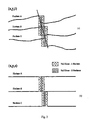
- Figure 1 shows, in a 2-D cross-section, the effects of dipping faults on this simple type of proportional slice for a pair of horizons.
- the output proportional slice volume is null or indeterminate at all (x,y) positions where one or both horizons is missing (e.g., Null Zone -1 Horizon in Figure 1 ),
- the proportional slice volume is also indeterminate for (x,y) positions where both horizons are present but on opposite sides of a dipping fault surface (e.g., Null Zone - 2 Horizons in Figure 1 ).
- One exemplary embodiment of the Domain Transform method of this invention explicitly requires interpreted horizons, faults, and other geologic surfaces as input, and, as a result, does not suffer the limitations of the method proposed by Lomask.
- Seismic-Wheeler Volumes represent interpreted depositional systems tracts as well as hiatuses in deposition based on horizon interpretations of system boundaries in 3-D. This approach requires recognition of the system tract by the interpreter as a starting point, and does not take into account the effects of post-depositional structural deformation and faulting.
- the implementations of Seismic-Wheeler Volumes described by Stark (2006) also depend on association of each seismic sample in the volume with a relative geologic time (Stark, 2004; Stark 2005a, US Patent 6,850,845 ; Stark 2005b, US Patent 6,853,922 ). This constraint is not present in the process described here.
- seismic data in a deformed volume can be interpreted in stratal-slice view.
- One exemplary goal is to reconstruct the data volume along stratal surfaces in an undeformed state using user-interpreted surfaces and user supplied information on geologic relationships in the volume as a guide. Seismic data in this undeformed state is more easily and accurately interpreted for stratigraphy, depositional systems, and depositional environments.
- volumetric data is often necessary for real-time rendering, for the segmentation of interpreted data, and for reducing visual clutter.
- a new Surface Wrapping technique has also been developed in accordance with an exemplary embodiment of this invention, and is described herein. For example, it allows, for example, the user to create a 3-D polygonal mesh that conforms to the exterior boundary of geobodies (such as stream channels) that offers significant improvements over existing techniques.
- Dorn's Surface Draping allows the user to view seismic data and define a series of points slightly above the desired horizon. These points define the initial shape of the 3-D mesh, which corresponds to the elastic sheet described above.
- the actual mesh is computed, generally using one vertex per voxel. These vertices are then iteratively "dropped" onto the horizon.
- the value of the voxel at each vertex's position is compared to a range that corresponds to the values found in an interpreted horizon. If the value falls within that range, the vertex is fixed in place.
- the Surface Draping concept would have benefits if adapted to work on geobodies and other 3-D volumes.
- Other approaches have been used to define a mesh that surrounds and conforms to the shape of a volume.
- Acosta et. al. 2006a and b; US Patents 7,006,085 and 7,098,908 ) propose a technique where the bounding surface is defined slice-by-slice by a user as a set of spline curves or general polylines that are then connected in 3-D.
- Kobbelt et, al. (1999) describes a technique based on successive subdivision of an initially simple mesh that completely surrounds the volume.
- the technique described by Koo et. al. (2005) improves on the same idea by allowing the user to define an arbitrarily shaped grid around a point cloud, allowing holes in the volume to be interpreted properly.
- Both of the above algorithms work by moving each vertex to the nearest point in the volume.
- an approach including a unique new workflow that includes a combination of existing and new novel processes is presented for computer-aided interpretation of depositional systems in 3-D seismic volumes.
- channels are used as the example of a depositional system, but the approach will work for the full range of depositional systems and environments recorded in 3-D seismic data volumes.
- This unique workflow includes the following general steps, illustrated in Figure 3a :
- Structural Interpretation refers to the interpretation of horizons and faults imaged in the 3-D seismic volume.
- the original seismic volume and its structural interpretation is typically described in an orthogonal cartesian coordinate system indicated by (x,y,z) or (x,y,t), where x and y represent horizontal distance, z represents vertical distance, and t typically represents vertical composite (also called two-way) reflection time.
- the proposed workflow can be applied to volumes that have been processed into either (x,y,z) or (x,y,t) volumes.
- Domain Transformation refers to a novel process of changing the coordinate space of the seismic volume from (x,y,z or t) to (x,y,s) where s represents "stratal-slice.”
- a stratal-slice is defined as a slice along an approximate paleo-depositional surface, that is, a surface upon which at some time in the past, geologic deposition (e.g., sedimentation or erosion) was occurring.
- the Domain Transformation creates a stratal-slice volume - a volume where every horizontal slice in the volume represents a stratal-slice or paleo depositional surface.
- This stratal-slice volume, created by the Domain Transformation process is a volume that is substantially free of deformation.
- This Domain Transformation process is unique in that it removes the effects of deformation that has occurred both during and subsequent to the deposition, and will properly construct a stratal-slice volume for all types of geologic surfaces and intervals.
- the Domain Transformation not only produces an ideal volume for the interpretation or extraction of elements of depositional systems, it also provides a valuable tool to highlight errors or omissions in the structural interpretation. Such errors or omissions are highlighted in the domain-transformed volume.
- Optional Structural Refinement uniquely enables the interpreter to correct these errors and omissions in either the (x,y,s) volume or the (x,y,z or t) volume and improve both the structural interpretation and the results of the Domain Transformation.
- Stratigraphic Interpretation encompasses both the processing of the Domain Transformed volume to improve the imaging of elements of depositional systems (herein referred to as attribute calculation), and the process of extracting the bounding surfaces of those elements of depositional systems.
- the bounding surface extraction process (herein referred to as Surface Wrapping) is a unique process that provides numerous advantages over processes currently practiced by individuals with ordinary skill in the art to obtain the bounding surfaces of elements of depositional systems, Surface Wrapping's applicability extends to the extraction of the bounding surfaces of bodies or aspects imaged in any type of volumetric data from any discipline.
- Inverse Domain Transformation refers to a process of changing the coordinate space of the seismic volume, any attribute volumes, the refined structural interpretation, and bounding surfaces from (x,y,s) to (x,y,z or t).
- Figure 1 shows simple proportional slicing for two horizons and a dipping fault surface: (a) data prior to proportional slicing; (b) data after proportional slicing.
- the null zones are regions where data is not properly handled by the simple proportional slice algorithm.
- Figure 2 shows simple proportional slicing for three horizons and a dipping fault surface: (a) data prior to proportional slicing; (b) data after proportional slicing. Note that the null data zones shift laterally between pairs of horizons due to the dip of the fault surface.
- Figure 3a is a flow diagram illustrating the exemplary general workflow and processes in performing automatic or semi-automatic interpretation of depositional systems in 3-D seismic data according to this invention.
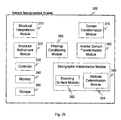
- Figure 3b illustrates an exemplary system capable of performing automatic or semi-automatic interpretation of depositional systems in 3-D seismic data according to this invention
- Figure 4 shows cross-sections of the Balmoral 3-D survey cutting across a 1 km wide deepwater turbidite channel.
- the section in (a) cuts the channel at an angle of 45°.
- the section in (b) cuts the channel at an angle of 90°.
- the edges of the channel are indicated by the vertical yellow arrows.
- Figure 5 is a horizon slice of seismic amplitude from the Balmoral 3-D survey.
- the 1 km wide deepwater turbidite channel cut by the channels in Figures 4a and 4b is readily visible in this slice.
- Figure 6 is a flow diagram illustrating the process of structural interpretation of 3-D seismic data in accordance with an exemplary embodiment of the invention
- Figure 7 shows a vertical section extracted from a 3-D seismic volume showing two interpreted horizons (labeled 1 and 2), and seven steeply dipping fault surfaces.
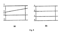
- Figure 8 shows a schematic cross-section of four intervals (A - D), two of which have laterally varying thickness (C and D) in (x,y,z) space in (a), and in the transformed domain (x,y,s) in (b).
- the "tick" marks illustrate the repositioning of input samples from the input volume to the output volume.
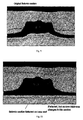
- Figure 9 shows the effects of the reefs presence as: (1) 'pull-up' of underlying horizons, and (2) truncation of horizontally adjacent horizons (not illustrated),
- Figure 10 shows that the velocity pull-up associated with the reef has been corrected
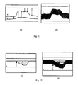
- Figure 11 is a schematic cross-section through a simple carbonate reef.
- the domain transformed equivalent is shown in (b) with the horizon at the base of the reef flattened, and the top reef retained.
- the shaded area in (b) represents null points in the transformed volume.
- Figure 12 illustrates a schematic cross-section through a canyon.
- a section through the input (x,y,z) space is shown in (a).
- a section through the (x,y,s) domain transformed space is shown in (b), Note that the canyon fill B and the layers above it are younger than the country rock A, and the paleo-depositional surfaces through the canyon fill are different that those in the surrounding country rock.
- the shaded area in (b) represents null points in the transformed volume.
- Figure 13 shows proportional slicing honoring dipping faults in 2-D for two horizons: (a) data prior to proportional slicing; (b) data after proportional slicing, By projecting slices in toward their intersection with the fault surface, the null zones are reduced to a narrower dipping zone centered on the fault surface.
- Figure 14 shows proportional slicing honoring dipping fault in 2-D for three horizons: (a) prior to proportional slicing; (b) data after proportional slicing.
- the narrow null data zone is continuous between intervals and is centered on the dipping fault surface.
- Figure 15 shows proportional slices honoring dipping faults in 3-D for two horizons: (a) data prior to proportional slicing; (b) data after proportional slicing. A final step, a horizontal shift, is added in (b) to account for the horizontal displacement along the fault surface.
- Figure 16 shows a schematic drawing of a simple faulted interval: (a) shows the interval in the input (x,y,z) space; (b) shows the interval in the transformed domain (x,y,s).
- the triangular regions adjacent to the fault require special handling in the transform.
- Figure 17 shows a schematic 3-D drawing of a faulted geologic volume with three layers in (x,y,z) space in (a); and the domain transformed version of the volume in (b).
- the fault has displacement down the fault surface (dip-slip) as well as a small amount of horizontal (strike-slip) displacement.
- the components of displacement are shown un the inset to (a) where ⁇ is the vertical dip-slip, ⁇ is the horizontal dip-slip, and ⁇ is the strike-slip component of displacement.
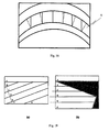
- Figure 18 shows a schematic drawing of a folded structure in a section in (x,y,z) space.
- the solid lines show the path for a vertical interpolation.
- the geologic interval may be better represented by an interpolation that is normal to the interval bounding surfaces, shown by the dashed lines.
- Figure 19 illustrates a schematic drawing of an angular unconformity (base of interval A) in (x,y,z) space in (a), and in the domain transformed volume in (b).
- the shaded area in (b) represents null space.
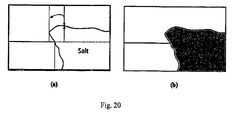
- Figure 20 illustrates a schematic drawing of a section through a salt body in (x,y,z) space in (a), and the corresponding section in the domain transformed space in (b).
- the shaded area in (b) represents null space.
- Figure 21 illustrates a flow diagram illustrating a high level view of the exemplary process of domain transformation of the seismic volume from the (x,y,z or t) domain to the (x,y,s) domain.
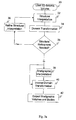
- Figure 22 illustrates a flow diagram illustrating the exemplary process of transform parameter calculation, a part of the domain transformation of seismic volumes.
- Figure 23 illustrates a flow diagram illustrating the exemplary process of forward domain transformation, a part of the domain transformation of seismic volumes
- Figure 24 illustrates an exemplary seismic volume before Domain Transformation (a), interpreted horizons and faults used in the transformation (b), and the Domain Transformed stratal-slice volume (c),
- the input seismic volume in (a) has deformation associated with syn and post depositional faulting.
- the output Domain Transformed volume (c) is substantially free of deformation.
- Figure 25 illustrates an exemplary Domain Transformed volume created from the volume in Figure 24a , using all of the 24 faults in Figure 24b , but using only two of the five horizons (the top-most and bottom-most horizons). With insufficient interpretive control, there is substantial deformation remaining in the volume.
- Figure 26 illustrates an exemplary flow diagram illustrating the process of refming the structural interpretation after initial domain transformation of the seismic volume.
- Figure 27 illustrates an exemplary flow diagram illustrating the process of inverse transformation of the refined structural interpretation from the transform domain to the domain of the original seismic volume. This process is part of the refinement of the structural interpretation illustrated in Figure 26 .
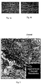
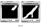
- Figure 28 illustrates a comparison of vertical and horizontal slices extracted from seismic volumes before and after domain transformation: (a) a vertical section and interpreted horizons and faults from the input seismic volume; (b) the corresponding vertical section from the domain transformed volume; (c) a horizontal slice from the input seismic volume showing a small portion of a stream channel (arrow in the lower right corner); (d) a horizontal slice from the domain transformed volume showing the full extent of the stream channel.
- Figure 29 illustrates an exemplary flow diagram illustrating the process of stratigraphic interpretation of the domain transformed volume.
- Figure 30 illustrates an exemplary defining of the initial bounding mesh (light grey) on a horizontal slice through the seismic volume, A channel-like object is imaged in the volume in darker grey.
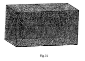
- Figure 31 illustrates an example of a very simple initial bounding surface mesh consisting of two abutting cubes.
- the exterior faces have been tessellated, while the two interior faces have been discarded.
- Figure 32 illustrates an example of an initial connected mesh defined by the surface wrapping process. Note that this mesh is from a different example than that used in Figure 30 .
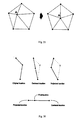
- Figure 33 illustrates two 2-D examples demonstrating the Surface Wrapping algorithm, showing an initial ring of connected vertices collapsing onto: (a) two rectangular objects; (b) a slice from an MRI (Magnetic Resonance Imaging) volume of a person's head.
- MRI Magnetic Resonance Imaging
- Figure 34 illustrates a 2-D diagram of fixed vertex determination in the Surface Wrapping algorithm.
- Figure 35 illustrates an exemplary method of determining the centralized vertex position in the Surface Wrapping algorithm.
- Figure 36 illustrates an exemplary method of determining the final vertex position based on the projected vertex position and centralized vertex position, using an elasticity factor of 0.8.
- Figure 37 illustrates a demonstration of the progression of several iterations of the surface wrapping algorithm, beginning with the initial bounding surface (upper left) and continuing to the detailed segmentation of the geobody (lower right).
- Figure 38 illustrates determining the "sharpness" of a vertex for simulation of a permeable surface in the Surface Wrapping algorithm.
- the magnitude of the sum of the surface vectors for a sharp vertex (left) is smaller than that of a blunt vertex (right).
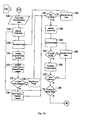
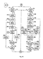
- Figure 39 illustrates an exemplary a flow diagram illustrating the process of surface wrapping of the elements of depositional systems. This process is part of the stratigraphic interpretation of the domain transformed volume illustrated in Figure 29 .
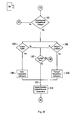
- Figure 40 illustrates an exemplary flow diagram of the process of inverse transformation from (x,y,s) to (x,y,z or t) of the surfaces and attribute volumes created in the stratigraphic interpretation process illustrated in Figures 29 and 39 .
- the various components of the system can be located at distant portions of a distributed network, such as a telecommunications network and/or the Internet, or within a dedicated secure, unsecured and/or encrypted system.
- a distributed network such as a telecommunications network and/or the Internet
- the components of the system can be combined into one or more devices or collocated on a particular node of a distributed network, such as a telecommunications network.
- the components of the system can be arranged at any location within a distributed network without affecting the operation of the system.
- links can be used to connect the elements and can be wired or wireless links, or any combination thereof, or any other known or later developed element(s) that is capable of supplying and/or communicating data to and from the connected elements.
- module as used herein can refer to any known or later developed hardware, software, firmware, or combination thereof that is capable of performing the functionality associated with that element.
- determine, calculate and compute, and variations thereof, as used herein are used interchangeably and include any type of methodology, process, mathematical operation or technique, including those performed by a system, such as an expert system or neural network.
- FIG. 3a shows an overall view of the CASI Workflow, the novel workflow proposed in this patent and Fig. 3b an architecture capable of performing the method.
- the seismic interpretation system 300 comprises a structural interpretation module 310, a structural refinement module 320, a controller 330, a memory 340, storage 350, a filtering/conditioning module 360, a domain transformation module 370, an inverse domain transformation module 380 and a stratigraphic interpretation module 390 which includes a bounding surface module 392 and an attribute determination module 394.
- the functions of the various components of the seismic interpretation system 300 will be discussed in relation to the following figures.
- a processed seismic data volume is loaded (30) into the computer for processing.
- This input seismic volume may have coordinate axes that are (x,y,z) or (x,y,t), where x, y, and z are spatial dimensions (e.g., with units of distance), where t is the measured one-way or two-way reflection time for the recorded seismic data, or where x, y, and z are simply indices incrementing or decrementing from initial values at the position defined as the origin of the volume.
- an interpreter can best recognize the existence of elements of depositional systems by looking at slices through the data that closely approximate paleo-depositional surfaces.
- the depositional elements are recognized in these slices from their characteristic morphology or shape, and can be readily recognized even if their presence is difficult or impossible to interpret from vertical sections of seismic data.
- Figures 4a and 4b show two vertical cross-sections taken from the 3-D survey.
- the sections cut across a 1 km wide deepwater turbidite channel.
- the section in Figure 4a is oriented at an angle of about 45 degrees to the direction of the channel.
- the section in Figure 4b is oriented at an angle of about 90 degrees to the channel. Even experienced interpreters might miss this large channel on vertical sections.
- Figure 5 is a horizon slice of seismic reflection amplitude through the channel.
- the existence, location, and direction of the channel are obvious from the horizon slice (in this case it is close to a stratal-slice), and it is readily identified based on the morphology (shape) of the channel.
- Figure 6 depicts a typical structural interpretation workflow (32).
- the input seismic volume from 30 is examined by the interpreter to determine if any additional data conditioning is required to achieve a reliable structural interpretation (decision 45). If decision 45 is "Yes", then the input data volume may be filtered to remove or minimize a variety of types of noise which may improve the structural interpretation (process 46, Structural Data Conditioning). This may include processes to remove random noise, coherent noise, or any artifacts from the volume that were introduced into or resulted from the seismic acquisition, and any processing steps preceding interpretation.
- Temporal (z or t axis 1-D filtering) includes, but is not limited to, high, low and band pass filtering, spectral shaping filters, and other trace filters commonly known to individuals schooled in the art of seismic processing and interpretation.
- Spatial (2-D) filters include, but are not limited to, mean and median filters, spatial wavelet filtering (e.g., using a Daubechies wavelet filter), and edge preserving filtering (Al-Dossary, et al., 2002; Jervis, 2006), and non-linear diffusion filtering (Imhof, 2003).
- 2-D spatial filters may operate on the volume along horizontal slices, or may be guided by local estimates of structural dip in the volume. In certain instances, the 2-D spatial filter operators may be extended into 3-D operators, depending on the type of data volume being filtered.
- Coherent noise in the volume may also need to be reduced by using a variety of coherent noise filtering techniques commonly know in the industry.
- the interpreter proceeds to the interpretation of horizons and faults in the volume of data.
- the interpretation of horizons and faults may be conducted manually, accomplished using automatic processes, or by any combination of manual and automatic techniques.
- the interpretation of horizons and faults may be conducted by interpreting horizons first, faults first, or by intermingling the interpretation of horizons and faults. Thus, the process of interpreting horizons and faults are shown in parallel in Figure 6 .
- Decision 47 represents the decision by the interpreter to interpret faults ("Yes") or not interpret faults ("No”).
- Decision 49 represents the decision by the interpreter to interpret horizons ("Yes") or not interpret horizons ("No”). If both decisions 47 and 49 are “No”, then decision 51 is "Yes” and the entire process and workflow is stopped, The workflow described here requires that either faults, or horizons, or both faults and horizons, be interpreted in the input seismic volume (30) or in the conditioned seismic volume (46), or some combination of the two volumes.
- FIG. 7 shows a typical vertical seismic section extracted from a 3-D seismic survey with two interpreted horizons (labeled 1 and 2 in Figure 7 ) and seven steeply dipping interpreted fault surfaces.
- geologic intervals and surfaces can be accommodated including, but not limited to:
- the process may also account for post-depositional structural geologic deformation including, but not limited to:
- the domain-transformation algorithm requires several types of data to be input. These include the seismic data volume, interpreted horizons and faults, and user input regarding horizon types and interval types. All transform changes to be performed are stored for each trace segment in the volume. These stored parameters consist of the starting time and sampling rate in the original volume, as well as the storage location in the stratal-volume and the number of sample to be interpolated during the forward transform process (62).
- the data volume is broken into several pieces for the purpose of Domain Transformation. There are two subdivisions used. The first is that each pair of user-supplied horizons defines an Interval. Each Interval may then contain one or more trace segments per trace location (an inline and crossline intersection). The trace segments are bounded by a user-supplied horizon and either a fault or another horizon (if no fault is present in that interval), or by two faults.
- the Domain Transformation is performed interval-by-interval through the volume.
- the calculation could proceed through the interpreted intervals in any order. In its preferred implementation, the calculations proceed from the shallowest interval to the deepest interval.
- the Domain Transformation interpolates the input seismic data following a set of geometric rules.
- the geometric rules are a function of the type of geologic interval on which the Domain Transformation is operating.
- the set of intervals included below is intended as a set of examples and is not inclusive of all the possible intervals that can be handled using the Domain Transformation approach. This subset is chosen for illustrative purposes. All types of geologic intervals can be handled using the approach presented for Domain Transformation.
- Proportional intervals include conformable intervals and growth intervals, with or without post-depositional folding and differential compaction.
- the maximum thickness for interval C is at the right edge, and the maximum thickness for interval B is at the left edge.
- the desired sample rate for every other trace in the interval is equal to the local thickness (Z L ) divided by the maximum number of samples (N).
- S L Z L / N
- This resampling of the input seismic volume may be accomplished by interpolation between the existing samples.
- the simple equations for determining the local desired sample rate S L guarantee that if a volume is forward transformed and then inverse transformed, none of the frequency content of the original volume will have been lost (i.e., the output sample rate is everywhere at least as frequent as the input sample rate, thereby preserving the frequency content, and avoiding aliasing problems).
- the first problem of a velocity pull-up is corrected by handling the strata immediately below the reef as if they were continuous flat surfaces.
- the second problem is corrected by assuming that the top reef structure should remain constant in the transformation (i.e., the shape of the top reef structure should be the same in the output stratal sliced volume as it is in the original input volume).
- the net result of these two corrections is that the base of the carbonate platform is flattened, eliminating velocity pull-ups, and the top structure is unchanged.
- the truncations of the clastic sedimentary layers against the top of the reef are maintained, and the reflections in the clastic section around the top reef structure are flattened.
- the manner of data extraction is demonstrated in Figure 11a .
- the overlying interval has trace segments extracted from the top down.
- the actual reef has trace segments extracted from the base upward.
- the maximum number of samples is calculated from the global maximum thickness (interval A + B).
- the maximum number of samples for the overlying interval A is equal to the maximum thickness of A divided by the sample rate of the input volume.
- the maximum number of samples for the reef interval B is calculated in a similar manner, with the additional step of multiplying the initial number of samples by a velocity-contrast correction factor.
- This velocity-contrast correction factor is the ratio of the seismic velocity of the carbonate reef divided by the seismic velocity of the overlying sediment. If this ratio is unknown, an assumed contrast (or no contrast at all) may be used.
- the local number of samples for each trace segment (above or below the top reef surface) is then calculated by multiplying that interval's maximum number of samples by the ratio of the local time thickness divided by the maximum time thickness of the interval.
- the resulting output section is shown Figure 11b .
- the shaded region represents a combination of the null regions output by both intervals, and is included in the Domain Transform output volume because the clastic sediments in interval A are geologically younger than the reef structure, interval B.
- reef correction is that continuous stratal slices can be output even when they are 'cut' by a reef. Data within the reef are stretched vertically in order to correct for the anomalous velocities within the reef ( Figures 10 and 11b ). This technique also works for other types of velocity anomalies (such as a gas zone).
- Figure 12a shows a schematic cross-section through a canyon in a seismic data volume.
- Figure 12b shows the same section through a Domain Transformed volume of the canyon.
- the stratal slices in the country rock (A) around the canyon and below the top of the canyon are handled independently of the stratal slices in the fill rock (B) in the canyon and above the top of the canyon. Because erosion had to occur to create the canyon, followed by later deposition of (B) the stratal slices are also separated by null data values in the domain transformed volume.
- the manner of data extraction begins by retaining the shape of the canyon unchanged in the transform.
- the overlying interval (B) has trace segments extracted from the top down, including the canyon fill.
- the country rock through which the canyon was cut by erosion (A) has trace segments extracted from bottom up.
- the maximum number of samples is calculated from the global maximum thickness (interval A + B).
- the maximum number of samples for the overlying interval A is equal to the maximum thickness of A divided by the sample rate of the input volume.
- the maximum number of samples for the canyon fill B is calculated in a similar manner.
- the local number of samples for each trace segment (above or below the top reef surface) is calculated by multiplying that interval's maximum number of samples by the ratio of the local time thickness divided by the maximum time thickness of the interval.
- the resulting output section is shown Figure 12b .
- the shaded region represents a combination of the null regions output by both intervals, and is included in the Domain Transform output volume because the clastic sediments in interval A are geologically older than the sediments in interval B,
- the result of canyon correction is that continuous stratal slices can be output even when they are 'cut' by a canyon,
- a faulted interval can be treated as a continuous interval where both the upper and lower bounding surfaces are present, However, difficulties arise in the vicinity of the fault where only one bounding surface is defined on either side of the fault ( Figures 1 and 2 ). In these fault zones, it becomes necessary to project the missing horizon inward to fill the fault zone with data points ( Figures 13 and 14 ).
- projection of the missing horizon is achieved by assuming that the time thickness in the fault zone is equal to the time thickness derived from the closest fully bound trace. This procedure takes place in two steps. First, an increasing radius search is performed in the (x,y) plane until the nearest trace is located that is bound by both horizons. Next, the time thickness is then calculated for this full trace, and assumed to be the same for the fault zone trace. This results in a projection where the missing horizon is assumed to be equidistant from the existing horizon in the fault zone. Honoring the horizontal component of dip-slip requires that data traces be shifted laterally in the (x,y) plane ( Figure 15 ).
- FIG 16 The manner of data extraction is illustrated in Figure 16 for a normal-offset fault.
- Other types of faults e.g., reverse-offset faults, thrust faults, and growth faults
- all trace segments may be handled as normal proportional interval trace segments.
- the local vertical thickness is estimated by fmding the closest fully-bounded trace segment on the same side of the fault (solid vertical lines between horizons A and B in Figure 16a ).
- the vertical thicknesses of the proximal complete trace segments (Z L and Z R ) are then used as estimates of the local vertical thicknesses that would be present in the zones ⁇ , and ⁇ were the fault not present.
- a number of samples which is less than the maximum number of samples for the interval is then output for the local trace segment for traces in the triangular shaped regions ( ⁇ and ⁇ ) in Figure 16a .
- the local number of samples (N L ) is calculated by multiplying the maximum number of samples (N) by the ratio of the thickness from the horizon to the fault (Z ⁇ and Z ⁇ ), divided by the local estimated vertical thickness.
- the estimation of the local vertical thickness that would be present in the zones ⁇ and ⁇ were the fault not present described above assumes a constant thickness of the interval AB in the region of the fault.
- a refinement of this approach is to determine both the vertical thickness of the proximal complete trace segment, and the gradient (rate of change or first derivative) of this thickness as the interval approaches the fault. Then, instead of projecting a constant thickness from the proximal trace toward the fault, the estimated thickness in zones ⁇ and ⁇ would be calculated from the thickness of the proximal trace segment plus a constant gradient of that thickness.
- Figure 17 is a 3-D diagram of a channel being cut by a fault.
- the fault exhibits both dip-slip (motion perpendicular to the long axis of the fault) and strike-slip (motion parallel to the long axis of the fault).
- Full closure of the fault requires handling both types of motion on the fault.
- the algorithm described for faults above compensates for the dip-slip component of fault motion.
- the strike-slip component of motion is handled by a horizontal adjustment of the voxels in the transformed volume on one side of the fault relative to the other.
- the amount of the adjustment may be calculated based on a number of criteria.
- the strike slip adjustment if required, is the lateral displacement along the fault required to minimize the difference in amplitude across the fault on any given output stratal slice. This type of operation is demonstrated in Figure 17b . After transformation, the channel is continuous and unbroken.
- the path through the volume for any point in the interval A in Figure 1 , 8 may be determined by several methods.
- Surface normals may be calculated for either the upper or lower bounding surfaces of interval A. If normals are calculated for the upper surface, then these normals would be projected down to their intersection with the lower surface at every point. If normals are calculated for the lower surface, then these normals would be projected up to their intersection with the upper surface at every point.
- a third, and perhaps better alternative, is to create a surface that is mid-way between the upper and lower interval bounding surfaces, calculate the surface normals to that intermediate surface, and extend those normals in each direction to the upper and lower bounding surfaces at every point.
- the projected normals define the path of interpolation in 3-D in the interval.
- Figure 19 demonstrates the modified handling of an interval containing an unconformity.
- the unconformity is the horizon at the base of interval A in the cross-section.
- the use of non-vertical traces (perpendicular to the bounding horizons) is shown in the pre-transform section on the left side of the figure by the dashed line.
- Intervals overlying an unconformity e.g., Interval A
- Intervals are treated in the normal proportional manner.
- intervals e.g., B - E
- the unconformity interval is handled in a manner similar to the foot wall of a fault.
- a search is performed to find the closest complete trace segment (both vertical and bed normal thickness are indicated in Figure 19a ).
- This trace segment is then used to calculate the approximate local thickness.
- the local number of output samples is calculated by multiplying the maximum number of samples by the ratio of the thickness from the horizon to the fault divided by the local approximate thickness. In the output section (shown on the right side of the figure), this results in the tapered configuration of the output interval.
- the shaded areas represent null regions, which are not represented in the input volume.
- FIG. 21 shows an overview of the Domain Transform process 34.
- Figure 22 shows the detailed flow of process 60, Transform Parameter Calculation, which is part of process 34.
- Figure 23 shows the detailed flow of process 62, Forward Domain Transformation, which is also part of process 34.
- the structural surfaces and geologic information provided by the interpreter regarding the types of geologic surfaces and intervals represented by the data are used to transform the seismic volume of data into a stratal-sliced volume.
- the Domain Transformation ideally removes all of the effects of structural deformation of the portion of the earth represented by the seismic volume. This results in a new seismic volume where each horizontal slice represents a paleo-depositional surface - a surface upon which deposition occurred at some time in the geologic past.
- the inputs to the Domain Transformation process (34) are the interpreted structure and seismic volume(s) (conditioned or not conditioned) from process 32. There may or may not be additional input to process 34 from process 36, Refine Structural Interpretation. Process 36 is shown in detail in Figure 26 and is described in detail below, after the description of process 34.
- decision 57 is made regarding conditioning of the input data (horizons, faults, and volumes) prior to process 60 (Transform Parameter Calculation). If decision 57 is "Yes", then the input data volume(s) and surfaces may be filtered to remove or minimize a variety of types of noise, thus improving the results of the Transform Parameter Calculation (process 60) and the results of the Forward Domain Transform (62).
- This may include processes to remove random noise, coherent noise, or any artifacts from the volume that were introduced or resulted from the seismic acquisition and processing steps preceding interpretation. Examples of such processes would include, but are not limited to, mean, median or wavelet filtering to the volume, and acquisition footprint removal. It is important to note that the actual techniques used to Condition Data in process 58 may differ from those used in process 46 to condition data for Structural Interpretation.
- Transform Parameter Calculation is input into process 60, Transform Parameter Calculation, which is described in detail in Figure 22 .
- the Transform Parameter Calculation process (60) also requires geologic information as input from the interpreter in 63.
- the interpreter should provide information regarding the types of geologic surfaces that are being input to process 60 and the types of geologic intervals that exist between the surfaces. This "geologic knowledge" is input into the algorithm in terms commonly used by individuals knowledgeable in the practice of seismic interpretation and geologic modeling.
- Such surfaces would include, but are not limited to, horizons, faults, unconformities, angular unconformities, and tops or bases of carbonate platforms.
- Intervals should include, but are not limited to, conformable intervals, growth intervals, and carbonate intervals.
- the Interval Index is initialized (64), the data for the first interval is obtained from the computer's memory (66, Get Interval Data), and the Maximum Interval Thickness is calculated (68).
- a Trace Segment is the portion of a seismic trace between the bounding surfaces that define an interval.
- the Trace Segment Index is initialized (70), and the Trace Segment is obtained from the volume.
- All Domain Transformation operations are performed once per trace segment present in the volume. For example, in a 3-D seismic volume with two interpreted horizons bounding one interval with no faults present, the number of trace segments will be equal to the number of inlines present in the volume multiplied by the number of cross-lines present in the volume. If there are three horizons present that define two unique intervals, the number of trace segments will be twice the single-interval case. Furthermore, if the same volume had faults present in the intervals to be Domain Transformed, the number of trace segments would increase by one for each fault at each inline and cross-line intersection that has a fault present inside a Domain Transformation interval.
- Any seismic Trace Segment in an interval between may be cut into one or more Sub-Segments by faults.
- decision 73 is made to determine if the trace is faulted in the interval. If the result of decision 73 is "Yes", then process 74 determines the Number of Sub-Segments into which the trace segment is cut by faults.
- the Trace Sub-Segment Index is initialized (76), and the Initial Trace Segment is obtained (78).
- Trace Sub-Segment Transform Parameters are calculated for each Sub-Segment in process 80. Decision 81 is evaluated to determine if there are More Sub-Segments on that Trace Segment in the interval.
- the Sub-Segment Index is incremented in process 82, the next Trace Sub-Segment is obtained (78), and its Trace Sub-Segment Transform Parameters are calculated (80). This continues until all sub-segments of the trace have been processed.
- the Trace Segment is input to process 83, and the Trace Segment Parameters are calculated.
- the Trace Segment and Trace Sub-Segment Transform Parameters are collected in process 84. These Transform Parameters define how each Trace Segment and Trace Sub-Segment must be processed in the Domain Transformation process to properly transform that segment or sub-segment given the definitions of the bounding geologic surfaces and the geologic interval containing that sub-segment.
- Decision 85 is evaluated to determine if there are more Trace Segments in the interval being processed. If the result of decision 85 is "Yes”, then the Trace Segment Index is incremented (86), the next Trace Segment is obtained (72), and decision 73 is evaluated for this new Trace Segment. If the result of decision 85 is "No”, then decision 87 is evaluated to determine if there are more intervals to process. If the answer to decision 87 is "Yes”, then the Interval Index is incremented (88), and the Interval Data for the next interval is retrieved (66).
- the Transform Displacement Volume is also created (89). This volume has the same dimensions as the output (re-sampled) Stratal Volume. Whereas the Stratal Volume stores the Domain Transformed version of the input data volume, the Transform Displacement Volume stores the x, y, and z coordinates of each data point in the Domain Transformed (x,y,s) volume. With this volume, the position of any interpretation produced from the Stratal Volume can be inverse transformed from (x,y,s) to the original (x,y,z) coordinates of the survey. Moreover, attribute volumes calculated from the stratal sliced volume can also be inverse transformed back to the original (x,y,z) coordinates as new 3-D attribute volumes.
- the data (including the seismic volume, horizons, faults, Transform Parameters, and Transform Displacement Volume) are passed from process 60 to process 62 ( Figure 23 ).
- the Transform Parameters stored by process 60 comprise the starting time and sample rate for each trace segment in the original input volume, as well as the number of samples to be interpolated and the location to store them in the Domain Transformed (stratal) output volume. These Transform Parameters are used to build the Stratal Volume by interpolating data points from the original input volume.
- the Transform Parameters calculated in process 60 are applied to the seismic volume, horizons and faults to transform the seismic volume and the surfaces from the (x,y,z) or (x,y,t) domain into the (x,y,s) domain, where s, the vertical dimension of the transformed data signifies "stratal-slice.”
- the first two steps in process 62 are Initialize the Interval Index (90) and Initialize the Trace Index in the Interval (92).
- Process 94 then retrieves the Local Trace Segment Parameters.
- Process 96 then calculates the Local Transformed Trace segment. Decision 97 is then made to determine if there are More Traces to be processed in the Interval.
- the type of interpolation performed by process 96 may be one of many established interpolation techniques. These techniques include, but are not limited to, linear interpolation, spline interpolation, and "sinc function" interpolation (also known as "(sin x)/x” interpolation). If interpolation is being performed in the trace (z or t) direction, the preferred implementation would use sine interpolation. In the case of interpolation along a 3-D path in the volume (e.g., because of steep dips), some combination of techniques may be used with the horizontal and vertical parts of the interpolation operation handled separately,
- the Transform Parameter Calculation process (60) outputs all of the input surfaces in Stratal-Domain coordinates. All types of surfaces are output as listed previously. Horizons are output as plantar features between the intervals that they separate in the Stratal Domain. Reef Tops are output with the same shape as they were input, but with their position following the interface between the extracted reef values and the null values that exist above the valid values. Similarly, salt boundaries and erosive surfaces are output along the interface of the valid data they bound and the null regions they define. These transformed surfaces act as a cue for the interpreter, indicating how the Stratal Domain volume relates to the input volume.
- the Domain Transformation produces a stratal-slice volume that is substantially free of any deformation. This deformation may have been caused by post or syn-depositional folding or faulting, differential compaction and/or differential sedimentation
- Figure 24a shows an input seismic volume in (x,y,t) space.
- the set of horizons and faults that were interpreted in the volume are shown in Fig. 24b
- the stratal-slice volume output by the Domain Transformation process in shown in Fig. 24c
- a total of five horizons and 24 faults were used in this transformation.
- the input volume shows substantial deformation from faulting, and from differential sedimentation (note the increasing thickness between interpreted horizons moving from the left edge of the image to the right edge.
- the output volume is substantially free of deformation, in that there are no significant remnant effects from the faulting or from the differential sedimentation.
- the reflection events in the stratal-sliced volume are all flat.
- Figure 25 shows a Domain Transformed volume, created from the input volume shown in Figure 24a using all of the interpreted faults, but only two of the five interpreted horizons shown in Fig. 24b .
- This Domain Transformed volume is not a stratal-sliced volume, in that it still retains a substantial amount of deformation from both faulting and from differential sedimentation, This deformation is most evident in the middle of the volume at the points that are farthest from the two bounding horizon surfaces that were used in the transformation.
- This volume clearly requires refinement of the structural interpretation (inclusion of additional interpreted horizons in this case). With insufficient interpretive control, there is substantial deformation remaining in the volume.
- decision 35 Figure 3a
- the Domain Transformed volume is examined for any of these errors and/or omissions. If Structural Refinement is needed (if decision 35 is "Yes") then process 36 is used to Refine the Structural Interpretation, thus correcting those errors and/or omissions. After this refinement process, the Domain Transformation (process 34) must be applied again in order for the refined structural interpretation to be applied in the transformation process.
- process 36 begins with a decision (101) to determine whether to Refine Structural in the Transformed Volume or in the original seismic volume. If decision 101 is evaluated as "No”, then control is passed to process 32 Structural Interpretation, and the structural refinement occurs in the original seismic volume using process 32, If decision 101 is evaluated as "Yes”, the structural refinement will be performed in process 36 on the domain transformed seismic volume.
- Data passed into process 36 from process 34 and decision 35 includes the domain transformed volume, the domain transformed surfaces (horizons, faults, etc.), and the Transform Displacement Volume.
- Structural refinement may involve the interpretation of additional horizons and/or faults, and may also include editing or changing the horizons or faults that were initially interpreted in process 32. This interpretation and editing may be conducted manually, accomplished using automatic processes, or by any combination of manual and automatic techniques. The interpretation of horizons and faults may be conducted by interpreting horizons first, faults first, or by intermingling the interpretation of horizons and faults. Thus, the processes of refining the interpretation of horizons and faults are shown in parallel in Figure 26 .
- Decision 103 represents the decision by the interpreter to interpret faults ("Yes") or not interpret faults ("No”).
- Decision 105 represents the decision by the interpreter to interpret horizons ("Yes") or not interpret horizons ("No”). If both decisions 103 and 105 are “No”, then decision 107 is "Yes” and the refinement process is stopped, and the transformed data and workflow passes on to process 38, Stratigraphic Interpretation. The workflow described here does not require that the interpretation be refined, even if a need for additional refinement of the structural interpretation is indicated by decision 35.
- decision 103 If decision 103 is "Yes”, then faults are interpreted and/or edited in the domain transformed seismic volumes (from 35) using any fault interpretation technique of the interpreter's choosing - either manual, automatic, or a combination of manual and automatic. If decision 105 is "Yes”, then horizons are interpreted and/or in the domain transformed seismic volumes (from 35) using any horizon interpretation technique of the interpreter's choosing - either manual, automatic, or a combination of manual and automatic.
- the refined structural interpretation if it is performed in the transformed volume in process 36, must be inverse transformed and merged with the original structural interpretation in process 32.
- the Inverse Transform of the Refined Structural Interpretation (process 112) is shown in detail in Figure 27 .
- Process 112 is the refined interpretation of faults and horizons (111), and the Transform Displacement Volume.
- Process 114 initializes the Surface Index, and the first Surface is obtained by process 116.
- Process 118 initializes the Point Index for points on the selected surface, and the first Point on the Surface is obtained by process 120.
- Process 122 is then used to convert the coordinates of the Point on the Surface from the transformed or stratal slice domain to the corresponding coordinates in the original domain of the seismic volume from 30.
- Decision 123 is then evaluated to determine whether there are More Points on the Surface. If decision 123 is evaluated as "Yes", then the Point Index is incremented by process 124, and the next Point on the Surface is obtained by process 120.
- decision 123 is evaluated as “No” (there are no more points on the current surface), then decision 125 is then evaluated to determine whether there are more surfaces. If decision 123 is evaluated as “Yes”, then process 126 increments the Surface Index, and the next Surface is obtained by process 116. If decision 123 is evaluated as "No”, then process 112 is completed and passes control back to process 34, to repeat the Domain Transformation of the original seismic volume using the refined structural interpretation.
- process 38 Stratigraphic Interpretation
- the purpose of the Stratigraphic Interpretation process is to assist the interpreter in the identification and interpretation of elements of depositional systems, or other seismic stratigraphic features represented in the Domain Transformed volume.
- the identification of these elements of depositional systems is accomplished by calculation of a variety of seismic attribute volumes within process 38. Once these elements of depositional systems have been identified in the attribute volumes, the bounding surfaces of these elements are also created in process 38.
- Figure 28 shows a comparison of slices extracted from an input seismic volume and a domain transformed volume. Five horizons and more than twenty faults were used in the domain transformation process applied to this volume.
- Figure 28a shows a vertical section extracted from the input seismic volume, with the fault surfaces and bounding horizons that intersect that section.
- Figure 28b shows the corresponding section extracted from the domain transformed volume. The arrows on Figure 28a show the points that correspond to the four corners of the section extracted from the domain transformed volume.
- Figures 28c and 28d respectively show 3-D views of horizontal slices taken through the input seismic volume and the domain transformed volume.
- the arrows indicate a channel on the two slices. In the input volume, only a small portion of the channel is visible on the horizontal slice because of the growth and faulting that is present in the volume. The entire channel is visible on the horizontal slice from the domain transformed volume because the effects of growth and faulting have been removed by the domain transformation process.
- the Domain Transformed seismic volume and Domain Transformed interpreted surfaces are input to process 38 (Stratigraphic Interpretation) from process 34 and decision 35 ( Figure 3a ).
- Process 38 is shown in detail in Figure 29 .
- decision 127 is evaluated to determine if the transformed data (both the transformed seismic volume and the interpreted surfaces) need to be conditioned prior to stratigraphic interpretation.
- the input transformed data volume and surfaces may be filtered to remove or minimize a variety of types of noise which may improve the stratigraphic interpretation (process 128, Stratigraphic Data Conditioning),
- This conditioning may include processes to remove random noise, coherent noise, or any artifacts from the volume that were introduced or resulted from the seismic acquisition and processing steps, or any noise or artifacts introduced in the Domain Transformation process (34). Examples of such processes would include, but are not limited to, mean, median or wavelet filtering to the volume, and acquisition footprint removal.
- a number of Stratigraphic Attribute Volumes may be calculated in process 130.
- the goal of calculating these attribute volumes is to produce through a single volume, or through a combination of volumes, a data volume or volumes that provide improved imaging of depositional systems when compared to the domain transformed seismic volume. Individuals practiced in the art of stratigraphic interpretation from 3-D seismic data are familiar with these attribute volumes.
- Attribute imaging of stratigraphy is improved by first transforming the seismic volume, and by then calculating the attribute volume in the transformed domain, This can be seen when compared to the typical practice of calculating the attributes directly on the input seismic volume without using domain transformation. Because of this, it is advantageous to provide the attribute volumes created by this workflow in the transform domain as output from process 38 to be inverse Transformed in process 40, as is shown in Figure 29 .
- decision 131 is evaluated to determine whether Multi-Attribute Imaging is going to be used to aid in the imaging of depositional systems using the attribute volumes. If decision 131 is evaluated as "Yes”, then process 132 is applied to identify optimum combinations of attributes to image the elements of depositional systems in the transformed space. There are a number of techniques in the industry that would be familiar to one who is practiced in the art of stratigraphic interpretation.
- neural network and neural network related techniques to analyze combinations of attributes for clusters that might identify elements of depositional systems (e.g., Kohonen Self-Organizing Maps and Growing Neural Gas), direct cluster analysis techniques (e,g., K-Means clustering), and techniques such as attribute cross-plot matrices and multi-dimensional attribute crossplot visualization techniques. Any of these techniques could be used in process 132 to image and analyze the multiple attribute volumes created by process 130 to image the depositional systems in the data.
- neural network and neural network related techniques to analyze combinations of attributes for clusters that might identify elements of depositional systems (e.g., Kohonen Self-Organizing Maps and Growing Neural Gas), direct cluster analysis techniques (e,g., K-Means clustering), and techniques such as attribute cross-plot matrices and multi-dimensional attribute crossplot visualization techniques. Any of these techniques could be used in process 132 to image and analyze the multiple attribute volumes created by process 130 to image the depositional systems in the data.
- an interpreter first specifies a range of voxel values that best isolates the voxels that correspond to the boundary of the intended geobody in the volume. The interpreter then defines an initial 3-D bounding surface which completely encloses the intended geobody and approximates its contours, isolating the voxels belonging to the geobody boundary from the rest of the volume.
- the initial bounding surface may be constructed using manual, automatic, or semi-automatic methods, or any combination thereof.
- the method for defining the initial bounding surface is based on a technique described by Kobbelt et, al. (1999). In this method, which is similar to graphical user interfaces that are commonly found in fully manual volume segmentation software, one slice of the volume is displayed on the screen, and the user defines the region contained by the initial bounding surface using a virtual brush to "paint" the region on the screen, as shown in Figure 30 .
- the interface used in Surface Wrapping is different in two ways.
- the painted region must fully enclose the boundary of the intended geobody (alternatively it must almost fill the boundary of the intended geobody), but need not precisely track the contour of the volume.
- the brush defines the same 2-D region on a user-defined range of slices simultaneously, thus extending the approximate bounding region into 3-D.
- the painted region is represented as a collection of cubes of equal dimensions, where each cube corresponds to a small portion of the volume that is contained within the initial bounding surface.
- Figure 31 shows two such adjacent cubes.
- the size of the cubes is globally adjustable by the user, the smaller the cube size, the denser the bounding surface mesh.
- the hull of the painted region is found by discarding cube faces that share the same spatial coordinates. The remaining faces are tessellated into two triangles per face, which collectively form the visible polygons of the bounding surface mesh ( Figure 31 ).
- An example of an initial mesh constructed from a large number of cubes is shown in Figure 32 .
- each vertex in the mesh maintains a record of its neighboring vertices, where a neighboring vertex is defined as any vertex to which it is directly connected by an edge of a triangle.
- a neighboring vertex is defined as any vertex to which it is directly connected by an edge of a triangle.
- Each vertex also maintains a record of all triangles of which it is a part.
- Vertex locations correspond to index coordinates relative to the data volume, and there may be at most one vertex data structure in the mesh at any given spatial coordinate, thus ensuring connectivity of vertices over the entire mesh.
- the Surface Wrapping process iteratively moves each vertex in the mesh toward the boundary of the intended geobody, as illustrated in 2-D in Figures 33a and 33b , wherein an initial ring of connected vertices collapses onto: (33a) two rectangular objects; (33b) a slice from an MRI (Magnetic Resonance Imaging) volume of a person's head.
- MRI Magnetic Resonance Imaging
- Each iteration of the surface wrapping algorithm begins with the calculation of the outward vertex normal vector for the first vertex in the mesh.
- the vertex normal is calculated as the normalized mean of the adjacent face normals, with a unit length corresponding to the grid spacing of the voxels in the data volume.
- N v is the magnitude of vector N v .
- a projected location for that vertex is then calculated to be at a point one unit length from the vertex's current position in the direction opposite to the outward unit normal at that vertex. If the initial mesh has been created everywhere inside the object whose boundary is sought, a projected location for that vertex is then calculated to be at a point one unit length from the vertex's current position in the direction of the outward unit normal at that vertex.
- the vertex is flagged as "fixed” ( Figure 34 ) and the projected location is not recorded. If the voxel value at the projected location does not fall within the specified range, the projected location is stored in the vertex data structure. This process is repeated for each vertex in the mesh, and is not order-dependent.
- a second location is computed for each non-fixed vertex, referred to here as the centralized location.
- the centralized location is determined to be the mean of the current locations of its neighboring vertices, as illustrated in Figure 35 . This process is repeated for each vertex in the mesh, and is not order-dependent.
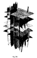
- Figure 37 illustrates the progression from top left to bottom right of successive iterations of this process as used to create a bounding surface mesh of a salt dome.
- vertex positions at each iteration may be pre-calculated prior to yielding control of the graphical interface to the user.
- a scroll bar a user can reveal the results of various vertex calculations and display them graphically. For example, by adjusting a scroll bar, a user could be presented with the series of images displayed in Fig. 37 .
- An additional feature that may be incorporated into the Surface Wrapping algorithm is the simulation of a semi-permeable surface, which allows outlying voxels to "push through" the mesh while maintaining the overall desired structure of the bounding surface. In the preferred implementation, this is accomplished by the use of an additional predicate immediately prior to the calculation of a vertex's projected location which determines if the vertex is creating a sharp point in the mesh. This predicate sums the surface normal vectors of the triangles that connect to the vertex and calculates the magnitude of the resulting vector. This calculation is illustrated in 2-D in Figure 38 , which shows the difference in the magnitude of the summed surface vectors for a sharp vertex versus a blunt vertex. If the magnitude is below a user-definable threshold, the vertex is flagged as non-fixed for the current iteration of the Surface Wrapping algorithm, which has the effect of smoothing out the spike in the mesh.
- the Surface Wrapping algorithm may also be applied to a subset of the vertices in the bounding surface mesh, allowing localized editing operation.
- a typical mechanism for selecting the affected vertices is any picking operation in a 3-D rendered view of the mesh, but the selection of vertices can be accomplished via any combination of manual or automatic techniques.
- process 148 Initializes the Vertex Index, and process 150 gets the initial Mesh Vertex.
- Process 152 calculates the Projected Vertex Location based on a movement of the vertex from its initial position along the direction of its unit normal toward the element of the depositional system.
- Process 154 then calculates an estimate of the Voxel Value at the Projected Vertex Location, Decision 155 (Voxel Value in Range) is evaluated to determine if the voxel has encountered the boundary of the depositional system or system element. If the Voxel Value is in the interpreter specified range (decision 155 evaluated as "Yes") then the vertex is Flagged as Fixed by process 158. If the Voxel Value is outside the interpreter specified range (decision 155 evaluated as "No") then process 156 Moves the Vertex to the Projected Location.
- decision 159 is evaluated to determine if there are More Vertices. If decision 159 evaluates as “Yes”, then process 160 Increments the Vertex Index, and process 150 gets the next Mesh Vertex. If decision 159 evaluates as "No”, then process 162 re-initializes the Vertex Index, and process 164 Gets the Mesh Vertex. Decision 165 is then evaluated to determine if the Vertex is Fixed. If decision 165 is evaluated as "Yes” (i.e., the vertex has been flagged as fixed) then process 168 Increments the Vertex Index, and process 164 Gets the next Mesh Vertex. If decision 165 is evaluated as "No” (i.e, the vertex has not been flagged as fixed) the process 166 Centralizes the Vertex Location with respect to the neighboring vertices in the mesh.
- decision 167 is evaluated to determine whether there are More Vertices in the mesh. If decision 167 is evaluated as “Yes” (i.e., there are more vertices), then process 168 Increments the Vertex Index, and process 164 Gets the next Mesh Vertex. If decision 167 is evaluated as "No” (i.e., there are no more vertices), then decision 169 is evaluated to determine whether to Continue Shrinking the Mesh. If decision 169 is evaluated as "Yes”, then process 148 Initializes the Vertex Index for the next shrinking step, and process 150 gets the Mesh Vertex, Note that once a vertex has been flagged as fixed in process 158, its projected position in process 154 remains fixed. If decision 169 is evaluated as "No”, then the surface mesh represents the bounding surface of the depositional system or system element to the conditions set by the interpreter at the beginning of the Surface Wrapping process (142),
- Process 40 requires as input information from the original seismic volume (30), from the Domain Transformation (34 through 35), and from the Stratigraphic Interpretation process (38).
- Data input into process 40 include the Domain Transformed Volume, attribute volumes calculated from the Domain Transformed Volume, the Domain Transformed Surfaces, all interpreted stratigraphic surfaces (either from manual interpretation or from Surface Wrapping), and the Transform Displacement Volume.
- the Inverse Transform process (40) is shown in detail in Figure 40 . Both attribute volumes and surfaces may be inverse transformed from the stratal slice domain into the spatial domain of the original input seismic volume (30).
- the workflows for surfaces and volumes are shown in parallel in Figure 40 for process 40.
- decisions 171 and 173 are evaluated. If decision 171 (Inverse Transform Surfaces) is evaluated as “Yes”, then the workflow for Inverse Transform of Surfaces is invoked. If decision 173 (Inverse Transform Volumes) is evaluated as "Yes”, then the workflow for Inverse Transform Volumes is invoked. If both decision 171 and decision 173 are evaluated as "No”, then all desired surfaces and volumes have been inverse transformed, and control is passed to process 42.
- the Inverse Transform process (40) allows interpretation produced in the Stratal Domain to be inverted back to the coordinates of the original volume. It also allows attributes that are produced with superior quality in the Stratal Domain to be inverted to the original coordinates.
- decision 171 is evaluated as "Yes” (Inverse Transform Surfaces)
- each point of the surfaces in the interpretation is inverted by finding its nearest neighbors in the Transform Displacement Volume. The original positions (in spatial coordinates) of these nearest neighbors are used to invert the position of that point.
- decision 173 is evaluated as "Yes", (Inverse Transform Volumes)
- each trace is re-sampled (stretched) back to the original coordinate using similar interpolation schemes to those described for the Forward Transform.
- process 174 initializes the Surface Index, and the first Surface is obtained by process 176.
- Process 178 initializes the Point Index for points on the selected surface, and the first Point on the Surface is obtained by process 180.
- Process 182 is then used to convert the coordinates of the Point on the Surface from the transformed or stratal slice domain to the corresponding coordinates in the original domain of the seismic volume from 30.
- Decision 181 is then evaluated to determine whether there are More Points on the Surface. If decision 181 is evaluated as "Yes”, then the Point Index is incremented by process 184, and the next Point on the Surface is obtained by process 180.
- decision 181 is evaluated as “No” (there are no more points on the current surface), then decision 183 is then evaluated to determine whether there are more surfaces. If decision 183 is evaluated as “Yes”, then process 186 increments the Surface Index, and the next Surface is obtained by process 176. If decision 183 is evaluated as "No”, the workflow for inverse transformation of surfaces is completed.
- process 188 initializes the Volume Index, and the first Volume is obtained by process 190.
- Process 192 initializes the Voxel Index for points in the selected volume, and the first Voxel in the Volume is obtained by process 194.
- Process 196 with additional input from process 35, Gets the Stratal Voxel Spatial Coordinates.
- Process 198 Gets the Stratal Voxel Value, and process 200, with additional input from process 30, Gets the Spatial Voxel Target Position in the inverse transformed volume.
- the results of processes 196, 198, and 200 are input into process 202, which then calculates the Voxel Value at the Target Position.
- Decision 201 is then evaluated to determine whether there are More Voxels in the Volume. If decision 201 is evaluated as “Yes”, then the Voxel Index is incremented by process 204, and the next Voxel in the Volume is obtained by process 194. If decision 201 is evaluated as "No” (there are no more voxels in the current volume), then decision 203 is then evaluated to determine whether there are more volumes. If decision 203 is evaluated as “Yes”, then process 206 increments the Volume Index, and the next Volume is obtained by process 190. If decision 203 is evaluated as "No”, the workflow for inverse transformation of volumes is completed.
- the output of the workflow (42) may include seismic attribute volumes, which were created in process 38 in the Domain Transformed coordinate system, and which have been Inverse Transformed by process 40 into the coordinate space of the input seismic volume (30).
- the output of the workflow (42) may also include the bounding surfaces of the interpreted elements of depositional systems, transformed by process 40 from surfaces in the coordinate space of the Domain Transformed volume, to the coordinate space of the input seismic volume (30).
- the systems, methods and techniques of this invention can be implemented on a special purpose computer, a programmed microprocessor or microcontroller and peripheral integrated circuit element(s), an ASIC or other integrated circuit, a digital signal processor, a hard-wired electronic or logic circuit such as discrete element circuit, a programmable logic device such as PLD, PLA, FPGA, PAL, any means, or the like.
- any device capable of implementing a state machine that is in turn capable of implementing the methodology illustrated herein can be used to implement the various communication methods and techniques according to this invention.
- the disclosed methods may be readily implemented in software using object or object-oriented software development environments that provide portable source code that can be used on a variety of computer or workstation platforms.
- the disclosed system may be implemented partially or fully in hardware using standard logic circuits or VLSI design. Whether software or hardware is used to implement the systems in accordance with this invention is dependent on the speed and/or efficiency requirements of the system, the particular function, and the particular software or hardware systems or microprocessor or microcomputer systems being utilized.
- the systems, methods and techniques illustrated herein can be readily implemented in hardware and/or software using any known or later developed systems or structures, devices and/or software by those of ordinary skill in the applicable art from the functional description provided herein and with a general basic knowledge of the computer and geologic arts.
- the disclosed methods may be readily implemented in software that can be stored on a storage medium, executed on programmed general-purpose computer with the cooperation of a controller and memory, a special purpose computer, a microprocessor, or the like.
- the systems and methods of this invention can be implemented as program embedded on personal computer such as an applet, JAVA® or CGI script, in C or C++, Fortran, or the like, as a resource residing on a server or computer workstation, as a routine embedded in a dedicated system or system component, or the like.
- the system can also be implemented by physically incorporating the system and/or method into a software and/or hardware system, such as the hardware and software systems of a dedicated seismic interpretation device.
Abstract
Description
- This application claims the benefit of and priority under 35 U.S.C. § 119(e) to
U.S. Patent Application Nos. 60/815,630, filed 21 June 2006 60/815,625, filed 21 June 2006 60/815,961, filed 21 June 2006 - An exemplary embodiment of this invention is in the field of 3-D interpretation, and more particularly to 3-D seismic interpretation. More specifically, an exemplary embodiment includes a workflow, including two new processes, implemented as software that is designed to enable automatic or semi-automatic interpretation of paleo-depositional features in three-dimensional seismic data for exploration, development and, for example, production of hydrocarbons.
- The need for computer-aided, semi-automatic and automatic interpretation of depositional systems derives from a combination of factors, Energy resources are becoming steadily more difficult to find and develop. It has been recognized for many years that the majority of new oil and gas reserves are a function of a complex combination of geological, structural and stratigraphic elements. While the problems of exploration and the efficient development of hydrocarbon reserves have become more difficult, the volume of data to be interpreted for each project has become orders of magnitude greater over the past 20 years. Simultaneously, both the number of interpreters and the time allowed for interpretation have been substantially reduced. This drives the need for more advanced computer-aided processes that can support the interpreter by enabling more efficient, precise and effective interpretation of 3-D seismic data volumes.
- Computer-aided structural interpretation of 3-D seismic data volumes has been embodied in tools in interactive seismic interpretation for a number of years. Since the early 1980s, horizon autotracking tools have been available to help increase the speed and consistency of horizon interpretation in 3-D seismic surveys (Dorn, 1998). More recently, techniques have been developed to provide computer-aided interpretation of faults and automatic fault interpretation (e.g.,
Crawford and Medwedeff, 1999, US Patent 5,987,388 ;Pederson, S. 1., 2002, US Patent 7,203,342 ), as well as techniques beyond event autotracking to automatically interpret horizons (Dorn, 1999, US Patent 5,894,417 ;Stark, 1997, US Patent 5,671,344 ), - Computer tools to aid in stratigraphic interpretation of seismic volumes have developed much more slowly, Elements of depositional systems can most readily be identified by an interpreter when the morphology of the paleo-depositional system can be viewed. Similarly, it is most likely that a computer algorithm can be written to recognize, image, and extract elements of depositional systems if the computer algorithm is able to operate on the data in a domain where the paleo-depositional system's morphology is most readily imaged. In both of these cases, the optimal environment is the stratal-slice domain, where the slices through the volume of seismic data are close approximations of paleo-depositional surfaces.
- In an undeformed data volume, horizontal slices (planar slices parallel to the (x,y) plane in the volume) may accurately represent depositional surfaces. However, in volumes with structural deformation, horizontal slices do not represent depositional surfaces for more than a small portion of the total volume. Faulting, folding, and velocity anomalies prevent the complete representation of such a surface by a simple horizontal slice.
- Horizon-slicing is defined as creating a slice through a 3-D seismic volume in the shape of an interpreted seismic reflection in that volume. Horizon slicing (as opposed to horizontal slicing) has provided better images of depositional systems since the mid-to-late 1980s,
- A continuous interval is a package of sediments that represent the same span of geologic age, but were deposited at different sedimentation rates in different parts of the volume. The result is an interval that represents that same amount of geologic time, but does not exhibit the same thickness. In such an interval, growth is caused by spatially variable rates of sedimentation. If we assume that sedimentation rates between a pair of bounding horizons are variable only in space (i.e., not vertically variable in a given location), stratal slices may be extracted by interpolating trace values vertically, where the interpolated sample interval at each (x,y) location is controlled by the upper and lower bounding surfaces and the number of samples desired in the interval on the output trace. This type of stratal slice has been referred to as a proportional slice.
- Proportional slicing or stratal slicing developed in the mid 1990s (Posamentier, et. al., 1996; Zeng, et. al. 1998a,b,c) provides even better imaging of depositional systems, and better discrimination between stacked channel systems in the seismic data because these surfaces are typically a better approximation of paleo-depositional surfaces than either horizon slices or horizontal slices.
- Zeng, et. al. (1998 a, b, c) describes the first instance of extracting slices based on geologic age. They reasoned that seismic reflectors do not always follow depositional surfaces. Thus, they interpolated seismic slices between surfaces judged to be time-equivalent. They referred to these interpolated slices as 'stratal' slices. Stark (2004) describes a similarly motivated effort. He used unwrapped phase as a proxy for user-interpreted age horizons. Slices were extracted from the data volume by drawing data from points of equal unwrapped phase. Stark's approach assumes that unwrapped phase closely approximates geologic age, but this is an assumption that is often in error.
- Both horizon slicing and proportional slicing generally suffer from substantial limitations in that they do not accommodate and compensate for generalized 3-D structural deformation subsequent to deposition, nor do they properly account for the wide variety of depositional environments. Horizon slicing is only appropriate for a conformable sequence of horizons in the seismic volume (i.e., a spatially uniform depositional environment over time). Proportional slicing is only appropriate for an interval that exhibits growth (i.e., a spatially gradational change in depositional thickness over an area, often due to spatially differential subsidence). Horizon and proportional slicing do not properly reconstruct paleo-depositional surfaces in other depositional environments, nor do they account for post-depositional structural changes (particularly faulting) or post-depositional erosion.
- Among the situations that the proportional or stratal slice volume (as defined by Zeng, et. al, 1998 a,b,c) does not handle properly are:
- Angular unconformities
- Non-linear growth in the interval between two horizons
- Carbonate platform intervals
- Faulting
- For example, both proportional slicing and stratal slicing (as defined by Zeng, et. al., 1998 a, b, c) produce volumes that have gaps or undefined zones where the volume is cut by a dipping fault surface.
Figure 1 shows, in a 2-D cross-section, the effects of dipping faults on this simple type of proportional slice for a pair of horizons. The output proportional slice volume is null or indeterminate at all (x,y) positions where one or both horizons is missing (e.g., Null Zone -1 Horizon inFigure 1 ), The proportional slice volume is also indeterminate for (x,y) positions where both horizons are present but on opposite sides of a dipping fault surface (e.g., Null Zone - 2 Horizons inFigure 1 ). - The situation for more than one pair of horizons is shown in
Figure 2 . In this case, there are null or indeterminate zones for each pair of horizons. These indeterminate zones are in different (x,y) positions for each pair of horizons. - In most previous attempts to solve this problem, where this simple form of proportional slicing is implemented, the indeterminate zones are filled with input seismic data rather than nulls, which can be quite misleading, Lomask et. al. (2006) have developed an approach that attempts to create a stratal volume without requiring interpreted horizons, faults or other surfaces to define and constrain the transformation. The lack of interpreted structural control in their approach produces poor results for seismic volumes that contain any significant structural deformation.
- One exemplary embodiment of the Domain Transform method of this invention explicitly requires interpreted horizons, faults, and other geologic surfaces as input, and, as a result, does not suffer the limitations of the method proposed by Lomask.
- Seismic-Wheeler Volumes (e.g., Stark, 2006) represent interpreted depositional systems tracts as well as hiatuses in deposition based on horizon interpretations of system boundaries in 3-D. This approach requires recognition of the system tract by the interpreter as a starting point, and does not take into account the effects of post-depositional structural deformation and faulting. The implementations of Seismic-Wheeler Volumes described by Stark (2006) also depend on association of each seismic sample in the volume with a relative geologic time (Stark, 2004;
Stark 2005a, US Patent 6,850,845 ;Stark 2005b, US Patent 6,853,922 ). This constraint is not present in the process described here. - By transforming seismic data from the (x,y,time/depth) domain to the (x,y,stratal-slice) domain, data in a deformed volume can be interpreted in stratal-slice view. One exemplary goal is to reconstruct the data volume along stratal surfaces in an undeformed state using user-interpreted surfaces and user supplied information on geologic relationships in the volume as a guide. Seismic data in this undeformed state is more easily and accurately interpreted for stratigraphy, depositional systems, and depositional environments.
- Finally, a lightweight representation of volumetric data is often necessary for real-time rendering, for the segmentation of interpreted data, and for reducing visual clutter. A new Surface Wrapping technique has also been developed in accordance with an exemplary embodiment of this invention, and is described herein. For example, it allows, for example, the user to create a 3-D polygonal mesh that conforms to the exterior boundary of geobodies (such as stream channels) that offers significant improvements over existing techniques.
- An inspiration for this Surface Wrapping approach was the Surface Draping algorithm (
Dorn, 1999, US Patent 5,894,417 ), which allows a polygonal mesh to be defined that reflects the geometry of an interpreted horizon. The surface draping algorithm is based on the metaphor of laying an elastic sheet over a contoured surface: gravity pulls the sheet down, causing it to conform to the surface beneath it, and the tension of the elastic material allows the sheet to smoothly cover small gaps in the surface while preserving the important features. - Dorn's Surface Draping allows the user to view seismic data and define a series of points slightly above the desired horizon. These points define the initial shape of the 3-D mesh, which corresponds to the elastic sheet described above. When the user has completed this stage, the actual mesh is computed, generally using one vertex per voxel. These vertices are then iteratively "dropped" onto the horizon. At each step, the value of the voxel at each vertex's position is compared to a range that corresponds to the values found in an interpreted horizon. If the value falls within that range, the vertex is fixed in place.
- The Surface Draping concept would have benefits if adapted to work on geobodies and other 3-D volumes. Other approaches have been used to define a mesh that surrounds and conforms to the shape of a volume.
Acosta et. al. (2006a and b; US Patents 7,006,085 and7,098,908 ) propose a technique where the bounding surface is defined slice-by-slice by a user as a set of spline curves or general polylines that are then connected in 3-D. Kobbelt et, al. (1999) describes a technique based on successive subdivision of an initially simple mesh that completely surrounds the volume. The technique described by Koo et. al. (2005) improves on the same idea by allowing the user to define an arbitrarily shaped grid around a point cloud, allowing holes in the volume to be interpreted properly. Both of the above algorithms work by moving each vertex to the nearest point in the volume. - It is an aspect of the present invention to provide a workflow and automated or semi-automated method and system for identifying and interpreting depositional environments, depositional systems and elements of depositional systems from 3-D seismic volumes.
- It is a further aspect of this invention to provide such a method and system in which noise in the seismic volume after acquisition and seismic processing is removed or minimized at each step in the workflow.
- It is a further aspect of this invention to provide a technique whereby the original 3-D seismic volume is transformed to a volume where every horizontal slice through the volume represents a paleo-depositional (stratal) surface, such that the effects of structural deformation are effectively removed from the volume.
- It is a further aspect of this invention to provide a means of imaging, recognizing and obtaining the bounding surfaces of depositional systems or elements of depositional systems in the transformed seismic volume.
- It is a further aspect of this invention to provide a technique whereby the imaging or attribute volumes created from the transformed seismic volume may be inverse-transformed to the coordinate space of the original seismic volume.
- It is a further aspect of this invention to provide a technique whereby the bounding surfaces obtained for depositional systems or elements of depositional systems obtained in the transformed seismic volume may be inverse-transformed to the coordinate space of the original seismic volume.
- In accordance with an exemplary embodiment of this invention, an approach including a unique new workflow that includes a combination of existing and new novel processes is presented for computer-aided interpretation of depositional systems in 3-D seismic volumes. In this discussion, channels are used as the example of a depositional system, but the approach will work for the full range of depositional systems and environments recorded in 3-D seismic data volumes.
- This unique workflow includes the following general steps, illustrated in
Figure 3a : - Load (Input) 3-D Seismic Volume
- Structural Interpretation
- Domain Transformation
- Optional Structural Refinement
- Stratigraphic Interpretation
- Inverse Domain Transformation
- Output Stratigraphic Volumes and Bodies
- Individual steps and series of steps of this workflow may be applied recursively to the data volume to improve the results of the overall process.
- Structural Interpretation refers to the interpretation of horizons and faults imaged in the 3-D seismic volume. The original seismic volume and its structural interpretation is typically described in an orthogonal cartesian coordinate system indicated by (x,y,z) or (x,y,t), where x and y represent horizontal distance, z represents vertical distance, and t typically represents vertical composite (also called two-way) reflection time. The proposed workflow can be applied to volumes that have been processed into either (x,y,z) or (x,y,t) volumes.
- Domain Transformation refers to a novel process of changing the coordinate space of the seismic volume from (x,y,z or t) to (x,y,s) where s represents "stratal-slice." A stratal-slice is defined as a slice along an approximate paleo-depositional surface, that is, a surface upon which at some time in the past, geologic deposition (e.g., sedimentation or erosion) was occurring. The Domain Transformation creates a stratal-slice volume - a volume where every horizontal slice in the volume represents a stratal-slice or paleo depositional surface. This stratal-slice volume, created by the Domain Transformation process, is a volume that is substantially free of deformation. This Domain Transformation process is unique in that it removes the effects of deformation that has occurred both during and subsequent to the deposition, and will properly construct a stratal-slice volume for all types of geologic surfaces and intervals.
- The Domain Transformation not only produces an ideal volume for the interpretation or extraction of elements of depositional systems, it also provides a valuable tool to highlight errors or omissions in the structural interpretation. Such errors or omissions are highlighted in the domain-transformed volume. Using the transformed volume to image problems in the structural interpretation, Optional Structural Refinement uniquely enables the interpreter to correct these errors and omissions in either the (x,y,s) volume or the (x,y,z or t) volume and improve both the structural interpretation and the results of the Domain Transformation.
- Stratigraphic Interpretation, as used here, encompasses both the processing of the Domain Transformed volume to improve the imaging of elements of depositional systems (herein referred to as attribute calculation), and the process of extracting the bounding surfaces of those elements of depositional systems. The bounding surface extraction process (herein referred to as Surface Wrapping) is a unique process that provides numerous advantages over processes currently practiced by individuals with ordinary skill in the art to obtain the bounding surfaces of elements of depositional systems, Surface Wrapping's applicability extends to the extraction of the bounding surfaces of bodies or aspects imaged in any type of volumetric data from any discipline.
- Inverse Domain Transformation refers to a process of changing the coordinate space of the seismic volume, any attribute volumes, the refined structural interpretation, and bounding surfaces from (x,y,s) to (x,y,z or t).
- As mentioned, individual steps and series of steps may be applied recursively to the data volume to improve the results of the overall process. For example, initial Structural Interpretation of key horizons and major faults followed by Stratal-slice Domain Transformation of the Seismic Volume may highlight secondary horizons or smaller faults (additional structural interpretation) that must be interpreted and honored in the Domain Transformation process to achieve higher quality results.
- Numerous exemplary benefits derive from the workflow and processes contained therein.
- Domain Transformation creates a stratal-sliced volume for any seismic volume of any structural complexity. Structural effects can be removed from the volume.
- An optimized view of stratigraphic features provides improved recognition and interpretation of depositional features.
- Stratigraphic features that are obscured by structural deformation in the input seismic volume are clearly imaged, recognizable, and interpretable in the transformed volume.
- A unique check and refinement of the structural interpretation is provided by the transformed volume (stratal-sliced volume), refinement of the structural interpretation (e.g., horizons and faults) in the stratal domain, and inverse Domain Transformation of the refined structural surfaces.
- This unique workflow integrates the structural and stratigraphic interpretations of the data in an internally self-consistent manner, not possible previously, thereby improving the quality of the interpretation.
- A novel Surface Wrapping technique provides a tool to obtain a connected, closed bounding surface for a 3-D object (geobody, stratigraphic feature, or any other arbitrary 3-D body) even where portions of the body are poorly imaged in the data volume.
- This Surface Wrapping technique has wide application to the extraction of complex 3-D bodies from any form of volumetric data. Applications would also include, but are not limited to, obtaining the bounding surfaces of complex 3-D salt bodies and canyons in seismic data, and obtaining the bounding surfaces of tissue structures imaged in 3-D medical imaging volumes (e.g., CT, MRJ, MRA, PET volumes, and the like).
- Seismic attributes that are determined using the Domain Transformed volume show a significant improvement both qualitatively and quantitatively when compared to the same attributes calculated using the original input seismic volume. The workflow of first transforming the volume, determining the attribute, and then inverse transforming the attribute volume produces markedly improved results when compared to directly determining the attribute on the input seismic volume.
- Attributes determined using the Domain Transformed volume improve the quality of the imaging of stratigraphy when compared to the same attributes determined using the input seismic volume:
- Improves the imaging of depositional systems
- Improves the correlation of attributes with well data for improved geophysical reservoir characterization.
- Since stratigraphic features are better imaged, more complete and more easily interpreted in the transformed domain, the workflow improves the efficiency, accuracy, and completeness of the interpretation of depositional systems when compared to other approaches.
- This Summary of the Invention is neither intended nor should it be construed as being representative of the full extent and scope of the present invention. While various embodiments of the present invention have been described in detail, it is apparent that modifications and alterations of those embodiments will occur to those skilled in the art. However, it is to be expressly understood that such modifications and alterations are within the scope and spirit of the present invention.
- These and other features and advantages of this invention are described in, or are apparent from, the following detailed description of the exemplary embodiments.
- The exemplary embodiments of the invention will be described in detail, with reference to the following figures. It should be understood that the drawings are not necessarily shown to scale. In certain instances, details which are not necessary for an understanding of the invention or which render other details difficult to perceive may have been omitted. It should be understood, of course, that the invention is not necessarily limited to the particular embodiments illustrated herein.
-
Figure 1 shows simple proportional slicing for two horizons and a dipping fault surface: (a) data prior to proportional slicing; (b) data after proportional slicing. The null zones are regions where data is not properly handled by the simple proportional slice algorithm. -
Figure 2 shows simple proportional slicing for three horizons and a dipping fault surface: (a) data prior to proportional slicing; (b) data after proportional slicing. Note that the null data zones shift laterally between pairs of horizons due to the dip of the fault surface. -
Figure 3a is a flow diagram illustrating the exemplary general workflow and processes in performing automatic or semi-automatic interpretation of depositional systems in 3-D seismic data according to this invention. -
Figure 3b illustrates an exemplary system capable of performing automatic or semi-automatic interpretation of depositional systems in 3-D seismic data according to this invention, -
Figure 4 shows cross-sections of the Balmoral 3-D survey cutting across a 1 km wide deepwater turbidite channel. The section in (a) cuts the channel at an angle of 45°. The section in (b) cuts the channel at an angle of 90°. The edges of the channel are indicated by the vertical yellow arrows. -
Figure 5 is a horizon slice of seismic amplitude from the Balmoral 3-D survey. The 1 km wide deepwater turbidite channel cut by the channels inFigures 4a and 4b is readily visible in this slice. -
Figure 6 is a flow diagram illustrating the process of structural interpretation of 3-D seismic data in accordance with an exemplary embodiment of the invention, -
Figure 7 shows a vertical section extracted from a 3-D seismic volume showing two interpreted horizons (labeled 1 and 2), and seven steeply dipping fault surfaces. -
Figure 8 shows a schematic cross-section of four intervals (A - D), two of which have laterally varying thickness (C and D) in (x,y,z) space in (a), and in the transformed domain (x,y,s) in (b). The "tick" marks illustrate the repositioning of input samples from the input volume to the output volume. -
Figure 9 shows the effects of the reefs presence as: (1) 'pull-up' of underlying horizons, and (2) truncation of horizontally adjacent horizons (not illustrated), -
Figure 10 shows that the velocity pull-up associated with the reef has been corrected, -
Figure 11 is a schematic cross-section through a simple carbonate reef. A section through the input (x,y,z) space in shown in (a) including a velocity "pull-up" of a horizon at the base of the reef. The domain transformed equivalent is shown in (b) with the horizon at the base of the reef flattened, and the top reef retained. The shaded area in (b) represents null points in the transformed volume. -
Figure 12 illustrates a schematic cross-section through a canyon. A section through the input (x,y,z) space is shown in (a). A section through the (x,y,s) domain transformed space is shown in (b), Note that the canyon fill B and the layers above it are younger than the country rock A, and the paleo-depositional surfaces through the canyon fill are different that those in the surrounding country rock. The shaded area in (b) represents null points in the transformed volume. -
Figure 13 shows proportional slicing honoring dipping faults in 2-D for two horizons: (a) data prior to proportional slicing; (b) data after proportional slicing, By projecting slices in toward their intersection with the fault surface, the null zones are reduced to a narrower dipping zone centered on the fault surface. -
Figure 14 shows proportional slicing honoring dipping fault in 2-D for three horizons: (a) prior to proportional slicing; (b) data after proportional slicing. The narrow null data zone is continuous between intervals and is centered on the dipping fault surface. -
Figure 15 shows proportional slices honoring dipping faults in 3-D for two horizons: (a) data prior to proportional slicing; (b) data after proportional slicing. A final step, a horizontal shift, is added in (b) to account for the horizontal displacement along the fault surface. -
Figure 16 shows a schematic drawing of a simple faulted interval: (a) shows the interval in the input (x,y,z) space; (b) shows the interval in the transformed domain (x,y,s). The triangular regions adjacent to the fault require special handling in the transform. -
Figure 17 shows a schematic 3-D drawing of a faulted geologic volume with three layers in (x,y,z) space in (a); and the domain transformed version of the volume in (b). The fault has displacement down the fault surface (dip-slip) as well as a small amount of horizontal (strike-slip) displacement. The components of displacement are shown un the inset to (a) where α is the vertical dip-slip, β is the horizontal dip-slip, and γ is the strike-slip component of displacement. -
Figure 18 shows a schematic drawing of a folded structure in a section in (x,y,z) space. The solid lines show the path for a vertical interpolation. The geologic interval may be better represented by an interpolation that is normal to the interval bounding surfaces, shown by the dashed lines. -
Figure 19 illustrates a schematic drawing of an angular unconformity (base of interval A) in (x,y,z) space in (a), and in the domain transformed volume in (b). The shaded area in (b) represents null space. -
Figure 20 illustrates a schematic drawing of a section through a salt body in (x,y,z) space in (a), and the corresponding section in the domain transformed space in (b). The shaded area in (b) represents null space. -
Figure 21 illustrates a flow diagram illustrating a high level view of the exemplary process of domain transformation of the seismic volume from the (x,y,z or t) domain to the (x,y,s) domain. -
Figure 22 illustrates a flow diagram illustrating the exemplary process of transform parameter calculation, a part of the domain transformation of seismic volumes. -
Figure 23 illustrates a flow diagram illustrating the exemplary process of forward domain transformation, a part of the domain transformation of seismic volumes, -
Figure 24 illustrates an exemplary seismic volume before Domain Transformation (a), interpreted horizons and faults used in the transformation (b), and the Domain Transformed stratal-slice volume (c), The input seismic volume in (a) has deformation associated with syn and post depositional faulting. The output Domain Transformed volume (c) is substantially free of deformation. -
Figure 25 illustrates an exemplary Domain Transformed volume created from the volume inFigure 24a , using all of the 24 faults inFigure 24b , but using only two of the five horizons (the top-most and bottom-most horizons). With insufficient interpretive control, there is substantial deformation remaining in the volume. -
Figure 26 illustrates an exemplary flow diagram illustrating the process of refming the structural interpretation after initial domain transformation of the seismic volume. -
Figure 27 illustrates an exemplary flow diagram illustrating the process of inverse transformation of the refined structural interpretation from the transform domain to the domain of the original seismic volume. This process is part of the refinement of the structural interpretation illustrated inFigure 26 . -
Figure 28 illustrates a comparison of vertical and horizontal slices extracted from seismic volumes before and after domain transformation: (a) a vertical section and interpreted horizons and faults from the input seismic volume; (b) the corresponding vertical section from the domain transformed volume; (c) a horizontal slice from the input seismic volume showing a small portion of a stream channel (arrow in the lower right corner); (d) a horizontal slice from the domain transformed volume showing the full extent of the stream channel. -
Figure 29 illustrates an exemplary flow diagram illustrating the process of stratigraphic interpretation of the domain transformed volume. -
Figure 30 illustrates an exemplary defining of the initial bounding mesh (light grey) on a horizontal slice through the seismic volume, A channel-like object is imaged in the volume in darker grey. -
Figure 31 illustrates an example of a very simple initial bounding surface mesh consisting of two abutting cubes. The exterior faces have been tessellated, while the two interior faces have been discarded. -
Figure 32 illustrates an example of an initial connected mesh defined by the surface wrapping process. Note that this mesh is from a different example than that used inFigure 30 . -
Figure 33 illustrates two 2-D examples demonstrating the Surface Wrapping algorithm, showing an initial ring of connected vertices collapsing onto: (a) two rectangular objects; (b) a slice from an MRI (Magnetic Resonance Imaging) volume of a person's head. -
Figure 34 illustrates a 2-D diagram of fixed vertex determination in the Surface Wrapping algorithm. -
Figure 35 illustrates an exemplary method of determining the centralized vertex position in the Surface Wrapping algorithm. -
Figure 36 illustrates an exemplary method of determining the final vertex position based on the projected vertex position and centralized vertex position, using an elasticity factor of 0.8. -
Figure 37 illustrates a demonstration of the progression of several iterations of the surface wrapping algorithm, beginning with the initial bounding surface (upper left) and continuing to the detailed segmentation of the geobody (lower right). -
Figure 38 illustrates determining the "sharpness" of a vertex for simulation of a permeable surface in the Surface Wrapping algorithm. The magnitude of the sum of the surface vectors for a sharp vertex (left) is smaller than that of a blunt vertex (right). -
Figure 39 illustrates an exemplary a flow diagram illustrating the process of surface wrapping of the elements of depositional systems. This process is part of the stratigraphic interpretation of the domain transformed volume illustrated inFigure 29 . -
Figure 40 illustrates an exemplary flow diagram of the process of inverse transformation from (x,y,s) to (x,y,z or t) of the surfaces and attribute volumes created in the stratigraphic interpretation process illustrated inFigures 29 and39 . - The exemplary embodiments of this invention will be described in relation to interpretation of data. However, it should be appreciated, that in general, the systems and methods of this invention will work equally well for any type of 3-D data (such as seismic data) from any environment.
- The exemplary systems and methods of this invention will also be described in relation to seismic interpretation, However, to avoid unnecessarily obscuring the present invention, the following description omits well-known structures and devices that may be shown in block diagram form or otherwise summarized.
- For purposes of explanation, numerous details are set forth in order to provide a thorough understanding of the present invention. However, it should be appreciated that the present invention may be practiced in a variety of ways beyond the specific details set forth herein.
- Furthermore, while the exemplary embodiments illustrated herein show the various components of the system collocated, it is to be appreciated that the various components of the system can be located at distant portions of a distributed network, such as a telecommunications network and/or the Internet, or within a dedicated secure, unsecured and/or encrypted system. Thus, it should be appreciated that the components of the system can be combined into one or more devices or collocated on a particular node of a distributed network, such as a telecommunications network. As will be appreciated from the following description, and for reasons of computational efficiency, the components of the system can be arranged at any location within a distributed network without affecting the operation of the system.
- Furthermore, it should be appreciated that various links can be used to connect the elements and can be wired or wireless links, or any combination thereof, or any other known or later developed element(s) that is capable of supplying and/or communicating data to and from the connected elements. The term module as used herein can refer to any known or later developed hardware, software, firmware, or combination thereof that is capable of performing the functionality associated with that element. The terms determine, calculate and compute, and variations thereof, as used herein are used interchangeably and include any type of methodology, process, mathematical operation or technique, including those performed by a system, such as an expert system or neural network.
- Additionally, all references identified herein are incorporated herein by reference in their entirely.
-
Figure 3a shows an overall view of the CASI Workflow, the novel workflow proposed in this patent andFig. 3b an architecture capable of performing the method. Theseismic interpretation system 300 comprises astructural interpretation module 310, astructural refinement module 320, acontroller 330, amemory 340,storage 350, a filtering/conditioning module 360, adomain transformation module 370, an inversedomain transformation module 380 and astratigraphic interpretation module 390 which includes a boundingsurface module 392 and anattribute determination module 394. The functions of the various components of theseismic interpretation system 300 will be discussed in relation to the following figures. - In this exemplary embodiment illustrated in
Fig. 3a , a processed seismic data volume is loaded (30) into the computer for processing. This input seismic volume may have coordinate axes that are (x,y,z) or (x,y,t), where x, y, and z are spatial dimensions (e.g., with units of distance), where t is the measured one-way or two-way reflection time for the recorded seismic data, or where x, y, and z are simply indices incrementing or decrementing from initial values at the position defined as the origin of the volume. - Philosophically, the approach is based on presenting the data to an interpreter and the computer processes in a manner that optimizes the imaging of depositional systems. For example, an interpreter can best recognize the existence of elements of depositional systems by looking at slices through the data that closely approximate paleo-depositional surfaces. The depositional elements are recognized in these slices from their characteristic morphology or shape, and can be readily recognized even if their presence is difficult or impossible to interpret from vertical sections of seismic data.
- For example,
Figures 4a and 4b show two vertical cross-sections taken from the 3-D survey. The sections cut across a 1 km wide deepwater turbidite channel. The section inFigure 4a is oriented at an angle of about 45 degrees to the direction of the channel. The section inFigure 4b is oriented at an angle of about 90 degrees to the channel. Even experienced interpreters might miss this large channel on vertical sections. -
Figure 5 is a horizon slice of seismic reflection amplitude through the channel. The existence, location, and direction of the channel are obvious from the horizon slice (in this case it is close to a stratal-slice), and it is readily identified based on the morphology (shape) of the channel. - Structural Interpretation
-
Figure 6 depicts a typical structural interpretation workflow (32). The input seismic volume from 30 is examined by the interpreter to determine if any additional data conditioning is required to achieve a reliable structural interpretation (decision 45). Ifdecision 45 is "Yes", then the input data volume may be filtered to remove or minimize a variety of types of noise which may improve the structural interpretation (process 46, Structural Data Conditioning). This may include processes to remove random noise, coherent noise, or any artifacts from the volume that were introduced into or resulted from the seismic acquisition, and any processing steps preceding interpretation. - Examples of such processes would include, but are not limited to, noise filtering of the data along the z or t axis (1-D filtering), spatial filtering along the (x,y) planes (2-D filtering), 3-D filter operators, and any combinations of these processes. Temporal (z or t axis 1-D filtering) includes, but is not limited to, high, low and band pass filtering, spectral shaping filters, and other trace filters commonly known to individuals schooled in the art of seismic processing and interpretation. Spatial (2-D) filters include, but are not limited to, mean and median filters, spatial wavelet filtering (e.g., using a Daubechies wavelet filter), and edge preserving filtering (Al-Dossary, et al., 2002; Jervis, 2006), and non-linear diffusion filtering (Imhof, 2003). 2-D spatial filters may operate on the volume along horizontal slices, or may be guided by local estimates of structural dip in the volume. In certain instances, the 2-D spatial filter operators may be extended into 3-D operators, depending on the type of data volume being filtered.
- The above filters are all designed to reduce the level of random noise in the seismic volume. Coherent noise in the volume (e.g., "acquisition footprint" - remnant features associated with the geometry used to acquire and process the seismic data) may also need to be reduced by using a variety of coherent noise filtering techniques commonly know in the industry.
- Once the input seismic volume (30) has been conditioned (46), or if no conditioning was necessary (i,e., the answer to
decision 45 was "No"), then the interpreter proceeds to the interpretation of horizons and faults in the volume of data. The interpretation of horizons and faults may be conducted manually, accomplished using automatic processes, or by any combination of manual and automatic techniques. The interpretation of horizons and faults may be conducted by interpreting horizons first, faults first, or by intermingling the interpretation of horizons and faults. Thus, the process of interpreting horizons and faults are shown in parallel inFigure 6 . -
Decision 47 represents the decision by the interpreter to interpret faults ("Yes") or not interpret faults ("No").Decision 49 represents the decision by the interpreter to interpret horizons ("Yes") or not interpret horizons ("No"). If bothdecisions decision 51 is "Yes" and the entire process and workflow is stopped, The workflow described here requires that either faults, or horizons, or both faults and horizons, be interpreted in the input seismic volume (30) or in the conditioned seismic volume (46), or some combination of the two volumes. - If
decision 47 is "Yes", then faults are interpreted from the seismic volumes (30 and/or 46) using any fault interpretation technique of the interpreter's choosing - either manual, automatic, or a combination of manual and automatic. Ifdecision 49 is "Yes", then horizons are interpreted from the seismic volumes (30 and/or 46) using any horizon interpretation technique of the interpreter's choosing - either manual, automatic, or a combination of manual and automatic.Figure 7 shows a typical vertical seismic section extracted from a 3-D seismic survey with two interpreted horizons (labeled 1 and 2 inFigure 7 ) and seven steeply dipping interpreted fault surfaces. - Once the interpreter has completed the interpretation of the horizons and faults of interest in
process 32 shown inFigures 3a and6 , then the seismic volume, and the interpreted structure (horizons and faults) are then passed into the Domain Transformation (process 34,Figure 3a ). - Domain Transformation
- Domain Transformation is a trace-by-trace approach to undoing the deforming effects of syn-depositional and post-depositional geologic processes. Syn-depositional processes take place at the same time, or as a result of, sediment deposition. Some examples of deformation resulting from these processes are differential deposition and differential compaction, The term "differential" implies variation in the horizontal direction. Post-depositional processes deform the rocks present after deposition of sediments has finished. Examples of these processes are faulting and folding of sediment layers, or the rock layers that eventually are formed by the aforementioned sediments.
- All types of geologic intervals and surfaces can be accommodated including, but not limited to:
- Continuous conformable intervals
- Continuous intervals that exhibit growth
- Intervals with reefs or carbonate platforms
- Unconformities (including angular unconformities) and disconformities
- Intervals with differential compaction
- The process may also account for post-depositional structural geologic deformation including, but not limited to:
- 3-D fault surfaces and displacement
- Folding
- Salt tectonics
- The domain-transformation algorithm requires several types of data to be input. These include the seismic data volume, interpreted horizons and faults, and user input regarding horizon types and interval types. All transform changes to be performed are stored for each trace segment in the volume. These stored parameters consist of the starting time and sampling rate in the original volume, as well as the storage location in the stratal-volume and the number of sample to be interpolated during the forward transform process (62).
- The data volume is broken into several pieces for the purpose of Domain Transformation. There are two subdivisions used. The first is that each pair of user-supplied horizons defines an Interval. Each Interval may then contain one or more trace segments per trace location (an inline and crossline intersection). The trace segments are bounded by a user-supplied horizon and either a fault or another horizon (if no fault is present in that interval), or by two faults.
- The Domain Transformation is performed interval-by-interval through the volume. The calculation could proceed through the interpreted intervals in any order. In its preferred implementation, the calculations proceed from the shallowest interval to the deepest interval. Within each interval, the Domain Transformation interpolates the input seismic data following a set of geometric rules. The geometric rules are a function of the type of geologic interval on which the Domain Transformation is operating.
- Example Intervals and Geometric Rules
- The set of intervals included below is intended as a set of examples and is not inclusive of all the possible intervals that can be handled using the Domain Transformation approach. This subset is chosen for illustrative purposes. All types of geologic intervals can be handled using the approach presented for Domain Transformation.
- Proportional Intervals:
- Proportional intervals include conformable intervals and growth intervals, with or without post-depositional folding and differential compaction. For continuous unfaulted proportional intervals, such as in
Figure 8 , three steps are performed. First, a global search is performed for all trace segments contained between the two bounding horizons. This search is meant to locate the thickest portion of the interval (ZM). The number of samples in this interval (N) at its maximum thickness is calculated by dividing this maximum time thickness by the sample rate (S) of the input data volume.
- In the case of
Figure 8 , the maximum thickness for interval C is at the right edge, and the maximum thickness for interval B is at the left edge. - For relatively shallow dips, and vertical re-sampling of the volume, the desired sample rate for every other trace in the interval is equal to the local thickness (ZL) divided by the maximum number of samples (N).

- This resampling of the input seismic volume may be accomplished by interpolation between the existing samples. The simple equations for determining the local desired sample rate SL guarantee that if a volume is forward transformed and then inverse transformed, none of the frequency content of the original volume will have been lost (i.e., the output sample rate is everywhere at least as frequent as the input sample rate, thereby preserving the frequency content, and avoiding aliasing problems).
- This resampling will result in thinner sections of the interval having a higher sample rate in the input (x,y,z) domain than in the thicker sections. The "tick" marks on the right and left side of
Figure 8a show schematically the relationship between thickness of the input interval and the desired relative locations in z and the sample rate to produce the output volume with stratal slices shown inFigure 8b . Note that the intervals inFigure 8b are constant in thickness, and that all samples are evenly spaced vertically in the output stratal slice domain. - All other intervals involve a generalization of this process described here for the proportional intervals.
- Carbonate Platform Interval:
- Carbonate reefs and the intervals that are immediately overly them require special handling. Intervals that contain carbonate reefs represent a two-fold problem. The first problem is that they represent a velocity anomaly that results in a velocity 'pull-up' of the underlying strata. The second problem is that they interrupt the horizontal continuity of adjacent intervals (
Figure 9 ). The transform algorithm must correct both of these issues. - The first problem of a velocity pull-up is corrected by handling the strata immediately below the reef as if they were continuous flat surfaces. The second problem is corrected by assuming that the top reef structure should remain constant in the transformation (i.e., the shape of the top reef structure should be the same in the output stratal sliced volume as it is in the original input volume). The net result of these two corrections (shown in
Figure 10 ) is that the base of the carbonate platform is flattened, eliminating velocity pull-ups, and the top structure is unchanged. The truncations of the clastic sedimentary layers against the top of the reef are maintained, and the reflections in the clastic section around the top reef structure are flattened. - The manner of data extraction is demonstrated in
Figure 11a . The overlying interval has trace segments extracted from the top down. The actual reef has trace segments extracted from the base upward. For both intervals, the maximum number of samples is calculated from the global maximum thickness (interval A + B). The maximum number of samples for the overlying interval A is equal to the maximum thickness of A divided by the sample rate of the input volume. The maximum number of samples for the reef interval B is calculated in a similar manner, with the additional step of multiplying the initial number of samples by a velocity-contrast correction factor. This velocity-contrast correction factor is the ratio of the seismic velocity of the carbonate reef divided by the seismic velocity of the overlying sediment. If this ratio is unknown, an assumed contrast (or no contrast at all) may be used. The local number of samples for each trace segment (above or below the top reef surface) is then calculated by multiplying that interval's maximum number of samples by the ratio of the local time thickness divided by the maximum time thickness of the interval. The resulting output section is shownFigure 11b . The shaded region represents a combination of the null regions output by both intervals, and is included in the Domain Transform output volume because the clastic sediments in interval A are geologically younger than the reef structure, interval B. - The result of reef correction is that continuous stratal slices can be output even when they are 'cut' by a reef. Data within the reef are stretched vertically in order to correct for the anomalous velocities within the reef (
Figures 10 and11b ). This technique also works for other types of velocity anomalies (such as a gas zone). - Canyon Intervals:
- Like carbonate reefs, intervals that include canyons require special handling. Although there typically is no velocity anomaly associated with the canyon, the sediment fill in the canyon is significantly younger, and belongs to different stratal slices than the "country rock" around the canyon.
-
Figure 12a shows a schematic cross-section through a canyon in a seismic data volume.Figure 12b shows the same section through a Domain Transformed volume of the canyon. The stratal slices in the country rock (A) around the canyon and below the top of the canyon are handled independently of the stratal slices in the fill rock (B) in the canyon and above the top of the canyon. Because erosion had to occur to create the canyon, followed by later deposition of (B) the stratal slices are also separated by null data values in the domain transformed volume. - The manner of data extraction begins by retaining the shape of the canyon unchanged in the transform. The overlying interval (B) has trace segments extracted from the top down, including the canyon fill. The country rock through which the canyon was cut by erosion (A) has trace segments extracted from bottom up. For both intervals, the maximum number of samples is calculated from the global maximum thickness (interval A + B). The maximum number of samples for the overlying interval A is equal to the maximum thickness of A divided by the sample rate of the input volume. The maximum number of samples for the canyon fill B is calculated in a similar manner. The local number of samples for each trace segment (above or below the top reef surface) is calculated by multiplying that interval's maximum number of samples by the ratio of the local time thickness divided by the maximum time thickness of the interval. The resulting output section is shown
Figure 12b . The shaded region represents a combination of the null regions output by both intervals, and is included in the Domain Transform output volume because the clastic sediments in interval A are geologically older than the sediments in interval B, The result of canyon correction is that continuous stratal slices can be output even when they are 'cut' by a canyon, - Faulted Intervals:
- A faulted interval can be treated as a continuous interval where both the upper and lower bounding surfaces are present, However, difficulties arise in the vicinity of the fault where only one bounding surface is defined on either side of the fault (
Figures 1 and2 ). In these fault zones, it becomes necessary to project the missing horizon inward to fill the fault zone with data points (Figures 13 and14 ). - Conceptually, projection of the missing horizon is achieved by assuming that the time thickness in the fault zone is equal to the time thickness derived from the closest fully bound trace. This procedure takes place in two steps. First, an increasing radius search is performed in the (x,y) plane until the nearest trace is located that is bound by both horizons. Next, the time thickness is then calculated for this full trace, and assumed to be the same for the fault zone trace. This results in a projection where the missing horizon is assumed to be equidistant from the existing horizon in the fault zone. Honoring the horizontal component of dip-slip requires that data traces be shifted laterally in the (x,y) plane (
Figure 15 ). - The manner of data extraction is illustrated in
Figure 16 for a normal-offset fault. Other types of faults (e.g., reverse-offset faults, thrust faults, and growth faults) may be processed in a similar fashion. Outside of the fault zone, all trace segments may be handled as normal proportional interval trace segments. However, in the fault zone, it is not possible to calculate the local time thickness in a normal manner as one horizon is missing (or exists on the other side of the fault). In these cases, the local vertical thickness is estimated by fmding the closest fully-bounded trace segment on the same side of the fault (solid vertical lines between horizons A and B inFigure 16a ). The vertical thicknesses of the proximal complete trace segments (ZL and ZR) are then used as estimates of the local vertical thicknesses that would be present in the zones α, and β were the fault not present. A number of samples which is less than the maximum number of samples for the interval is then output for the local trace segment for traces in the triangular shaped regions (α and β) inFigure 16a . The local number of samples (NL) is calculated by multiplying the maximum number of samples (N) by the ratio of the thickness from the horizon to the fault (Zα and Zβ), divided by the local estimated vertical thickness.
- These samples are interpolated from the top down for the hanging wall of the fault, and from the bottom up for the foot wall. The output interval in
Figure 16b has the same total thickness throughout. The vertical dashed lines inFigure 16b indicate the section of the interval that received special fault handling. - The estimation of the local vertical thickness that would be present in the zones α and β were the fault not present described above assumes a constant thickness of the interval AB in the region of the fault. A refinement of this approach is to determine both the vertical thickness of the proximal complete trace segment, and the gradient (rate of change or first derivative) of this thickness as the interval approaches the fault. Then, instead of projecting a constant thickness from the proximal trace toward the fault, the estimated thickness in zones α and β would be calculated from the thickness of the proximal trace segment plus a constant gradient of that thickness.
- Real faulting is commonly more complex than 2-D diagrams would imply.
Figure 17 is a 3-D diagram of a channel being cut by a fault. The fault exhibits both dip-slip (motion perpendicular to the long axis of the fault) and strike-slip (motion parallel to the long axis of the fault). Full closure of the fault requires handling both types of motion on the fault. - The algorithm described for faults above, compensates for the dip-slip component of fault motion. The strike-slip component of motion is handled by a horizontal adjustment of the voxels in the transformed volume on one side of the fault relative to the other. The amount of the adjustment may be calculated based on a number of criteria. In its simplest form, the strike slip adjustment, if required, is the lateral displacement along the fault required to minimize the difference in amplitude across the fault on any given output stratal slice. This type of operation is demonstrated in
Figure 17b . After transformation, the channel is continuous and unbroken. - Interpolation for Steeply Dipping Intervals
- The interpolation that has been described above (interpolation of traces vertically) works well for all cases except those that involve steeply dipping intervals. In steeply dipping intervals, extracting data vertically from the input volume is not a sufficient approximation of the geology present in the volume. Correct handling of steeply dipping intervals requires the use of non-vertical data traces, as can be seen in
Figure 18 . This figure represents a folded interval that contains a flat top and dipping flanks. The solid lines indicate vertical traces. The dashed lines indicate traces that are correctly oriented perpendicularly to the interval's bounding horizons. The difference between the two methods of data extraction becomes greater as dip increases on the flanks of the structure. Thus, these types of intervals require interpolation through the volume along paths that are non-vertical. - The path through the volume for any point in the interval A in
Figure 1 ,8 may be determined by several methods. Surface normals may be calculated for either the upper or lower bounding surfaces of interval A. If normals are calculated for the upper surface, then these normals would be projected down to their intersection with the lower surface at every point. If normals are calculated for the lower surface, then these normals would be projected up to their intersection with the upper surface at every point. A third, and perhaps better alternative, is to create a surface that is mid-way between the upper and lower interval bounding surfaces, calculate the surface normals to that intermediate surface, and extend those normals in each direction to the upper and lower bounding surfaces at every point. - Whichever method is used to calculate and project the surface normals, the projected normals define the path of interpolation in 3-D in the interval.
- Unconformities:
-
Figure 19 demonstrates the modified handling of an interval containing an unconformity. The unconformity is the horizon at the base of interval A in the cross-section. The use of non-vertical traces (perpendicular to the bounding horizons) is shown in the pre-transform section on the left side of the figure by the dashed line. Intervals overlying an unconformity (e.g., Interval A) are treated in the normal proportional manner. Beneath the unconformity, intervals (e.g., B - E) are also handled in the normal proportional manner away from the unconformity surface where both bounding horizons for each interval are present. - In the presence of the unconformity, the unconformity interval is handled in a manner similar to the foot wall of a fault. A search is performed to find the closest complete trace segment (both vertical and bed normal thickness are indicated in
Figure 19a ). This trace segment is then used to calculate the approximate local thickness. As with fault handling, the local number of output samples is calculated by multiplying the maximum number of samples by the ratio of the thickness from the horizon to the fault divided by the local approximate thickness. In the output section (shown on the right side of the figure), this results in the tapered configuration of the output interval. The shaded areas represent null regions, which are not represented in the input volume. - Salt Boundaries:
- Many seismic volumes contain complex 3-D salt bodies. Intervals that are partially bounded by salt are handled in a manner similar to faults and to reef top boundaries. As with faults, trace segments that are fully bounded by non-salt horizons are handled in the normal proportional manner. Where a trace segment is bounded by the salt boundary and a non-salt horizon, a search must be made for the closest full non-salt bounded trace segment. As with fault handling, the thickness from this proximal fully-bounded trace segment is used to determine the number of samples to be output in the local trace segment. This number of samples is equal to the maximum number of samples multiplied by the ratio of the thickness between the salt and non-salt horizons divided by the thickness of the fully-bounded trace segment. The resulting output of this interval is demonstrated in
Figure 20 . The shape of the salt horizon is preserved, while removing complexities and growth that exist due to the non-salt horizons. - Domain Transformation Specification and Determination
- The Domain Transformation process described above is implemented as process 34 (
Figure 3a ) and is shown in detail inFigures 21 ,22 and23 .Figure 21 shows an overview of theDomain Transform process 34.Figure 22 shows the detailed flow ofprocess 60, Transform Parameter Calculation, which is part ofprocess 34.Figure 23 shows the detailed flow ofprocess 62, Forward Domain Transformation, which is also part ofprocess 34. - In Domain Transformation, the structural surfaces and geologic information provided by the interpreter regarding the types of geologic surfaces and intervals represented by the data are used to transform the seismic volume of data into a stratal-sliced volume. The Domain Transformation ideally removes all of the effects of structural deformation of the portion of the earth represented by the seismic volume. This results in a new seismic volume where each horizontal slice represents a paleo-depositional surface - a surface upon which deposition occurred at some time in the geologic past.
- The inputs to the Domain Transformation process (34) are the interpreted structure and seismic volume(s) (conditioned or not conditioned) from
process 32. There may or may not be additional input to process 34 fromprocess 36, Refine Structural Interpretation.Process 36 is shown in detail inFigure 26 and is described in detail below, after the description ofprocess 34. - Upon input of data to process 34, decision 57 (Condition Data) is made regarding conditioning of the input data (horizons, faults, and volumes) prior to process 60 (Transform Parameter Calculation). If
decision 57 is "Yes", then the input data volume(s) and surfaces may be filtered to remove or minimize a variety of types of noise, thus improving the results of the Transform Parameter Calculation (process 60) and the results of the Forward Domain Transform (62). This may include processes to remove random noise, coherent noise, or any artifacts from the volume that were introduced or resulted from the seismic acquisition and processing steps preceding interpretation. Examples of such processes would include, but are not limited to, mean, median or wavelet filtering to the volume, and acquisition footprint removal. It is important to note that the actual techniques used to Condition Data inprocess 58 may differ from those used inprocess 46 to condition data for Structural Interpretation. - Once the input volume(s) and surfaces (32) have been conditioned (58), or if no conditioning is necessary (i.e., the answer to
decision 57 was "No"), then these data (represented inFigure 21 by 59) axe input intoprocess 60, Transform Parameter Calculation, which is described in detail inFigure 22 . The Transform Parameter Calculation process (60) also requires geologic information as input from the interpreter in 63. The interpreter should provide information regarding the types of geologic surfaces that are being input to process 60 and the types of geologic intervals that exist between the surfaces. This "geologic knowledge" is input into the algorithm in terms commonly used by individuals knowledgeable in the practice of seismic interpretation and geologic modeling. Such surfaces would include, but are not limited to, horizons, faults, unconformities, angular unconformities, and tops or bases of carbonate platforms. Intervals should include, but are not limited to, conformable intervals, growth intervals, and carbonate intervals. - Once all of the requisite input has been supplied, the Interval Index is initialized (64), the data for the first interval is obtained from the computer's memory (66, Get Interval Data), and the Maximum Interval Thickness is calculated (68). A Trace Segment is the portion of a seismic trace between the bounding surfaces that define an interval. The Trace Segment Index is initialized (70), and the Trace Segment is obtained from the volume.
- All Domain Transformation operations are performed once per trace segment present in the volume. For example, in a 3-D seismic volume with two interpreted horizons bounding one interval with no faults present, the number of trace segments will be equal to the number of inlines present in the volume multiplied by the number of cross-lines present in the volume. If there are three horizons present that define two unique intervals, the number of trace segments will be twice the single-interval case. Furthermore, if the same volume had faults present in the intervals to be Domain Transformed, the number of trace segments would increase by one for each fault at each inline and cross-line intersection that has a fault present inside a Domain Transformation interval.
- Any seismic Trace Segment in an interval between may be cut into one or more Sub-Segments by faults. Thus, once the Trace Segment has been obtained,
decision 73 is made to determine if the trace is faulted in the interval. If the result ofdecision 73 is "Yes", then process 74 determines the Number of Sub-Segments into which the trace segment is cut by faults. The Trace Sub-Segment Index is initialized (76), and the Initial Trace Segment is obtained (78). Trace Sub-Segment Transform Parameters are calculated for each Sub-Segment inprocess 80.Decision 81 is evaluated to determine if there are More Sub-Segments on that Trace Segment in the interval. If the result ofdecision 81 is "Yes", the Sub-Segment Index is incremented inprocess 82, the next Trace Sub-Segment is obtained (78), and its Trace Sub-Segment Transform Parameters are calculated (80). This continues until all sub-segments of the trace have been processed. - If the result of
decision 73 is "No", then the Trace Segment is input to process 83, and the Trace Segment Parameters are calculated. The Trace Segment and Trace Sub-Segment Transform Parameters are collected inprocess 84. These Transform Parameters define how each Trace Segment and Trace Sub-Segment must be processed in the Domain Transformation process to properly transform that segment or sub-segment given the definitions of the bounding geologic surfaces and the geologic interval containing that sub-segment. -
Decision 85 is evaluated to determine if there are more Trace Segments in the interval being processed. If the result ofdecision 85 is "Yes", then the Trace Segment Index is incremented (86), the next Trace Segment is obtained (72), anddecision 73 is evaluated for this new Trace Segment. If the result ofdecision 85 is "No", thendecision 87 is evaluated to determine if there are more intervals to process. If the answer todecision 87 is "Yes", then the Interval Index is incremented (88), and the Interval Data for the next interval is retrieved (66). - These processes continue until Transform Parameters have been calculated for all Trace Sub-Segments and Trace Segments in all Intervals. While calculating the trace segments the Transform Displacement Volume is also created (89). This volume has the same dimensions as the output (re-sampled) Stratal Volume. Whereas the Stratal Volume stores the Domain Transformed version of the input data volume, the Transform Displacement Volume stores the x, y, and z coordinates of each data point in the Domain Transformed (x,y,s) volume. With this volume, the position of any interpretation produced from the Stratal Volume can be inverse transformed from (x,y,s) to the original (x,y,z) coordinates of the survey. Moreover, attribute volumes calculated from the stratal sliced volume can also be inverse transformed back to the original (x,y,z) coordinates as new 3-D attribute volumes.
- Forward Domain Transformation
- Once
process 60 is complete, the data (including the seismic volume, horizons, faults, Transform Parameters, and Transform Displacement Volume) are passed fromprocess 60 to process 62 (Figure 23 ). The Transform Parameters stored byprocess 60 comprise the starting time and sample rate for each trace segment in the original input volume, as well as the number of samples to be interpolated and the location to store them in the Domain Transformed (stratal) output volume. These Transform Parameters are used to build the Stratal Volume by interpolating data points from the original input volume. - In process 62 (
Figure 23 ), the Transform Parameters calculated inprocess 60 are applied to the seismic volume, horizons and faults to transform the seismic volume and the surfaces from the (x,y,z) or (x,y,t) domain into the (x,y,s) domain, where s, the vertical dimension of the transformed data signifies "stratal-slice." The first two steps inprocess 62 are Initialize the Interval Index (90) and Initialize the Trace Index in the Interval (92).Process 94 then retrieves the Local Trace Segment Parameters.Process 96 then calculates the Local Transformed Trace segment. Decision 97 is then made to determine if there are More Traces to be processed in the Interval. If the result of decision 97 is "Yes", then the Trace Index is incremented (98) and the Transform Parameters are retrieved for the next Local Trace Segment (94). If the result of decision 97 is "No", thendecision 99 is evaluated to determine if there are more intervals to be processed. If the result ofdecision 99 is "Yes", the Interval Index is incremented (100), and the Trace Index in the Interval is initialized (92).Process 62 continues in this manner until all trace segments in all intervals have been transformed to the (x,y,s) domain. - The type of interpolation performed by
process 96 may be one of many established interpolation techniques. These techniques include, but are not limited to, linear interpolation, spline interpolation, and "sinc function" interpolation (also known as "(sin x)/x" interpolation). If interpolation is being performed in the trace (z or t) direction, the preferred implementation would use sine interpolation. In the case of interpolation along a 3-D path in the volume (e.g., because of steep dips), some combination of techniques may be used with the horizontal and vertical parts of the interpolation operation handled separately, - The Transform Parameter Calculation process (60) outputs all of the input surfaces in Stratal-Domain coordinates. All types of surfaces are output as listed previously. Horizons are output as plantar features between the intervals that they separate in the Stratal Domain. Reef Tops are output with the same shape as they were input, but with their position following the interface between the extracted reef values and the null values that exist above the valid values. Similarly, salt boundaries and erosive surfaces are output along the interface of the valid data they bound and the null regions they define. These transformed surfaces act as a cue for the interpreter, indicating how the Stratal Domain volume relates to the input volume.
- When sufficient structural control in the form of interpreted horizons, faults, salt boundaries, canyon boundaries, and other possible geological surfaces is used, the Domain Transformation produces a stratal-slice volume that is substantially free of any deformation. This deformation may have been caused by post or syn-depositional folding or faulting, differential compaction and/or differential sedimentation
-
Figure 24a shows an input seismic volume in (x,y,t) space. The set of horizons and faults that were interpreted in the volume are shown inFig. 24b , and the stratal-slice volume output by the Domain Transformation process in shown inFig. 24c , A total of five horizons and 24 faults were used in this transformation. The input volume shows substantial deformation from faulting, and from differential sedimentation (note the increasing thickness between interpreted horizons moving from the left edge of the image to the right edge. - The output volume is substantially free of deformation, in that there are no significant remnant effects from the faulting or from the differential sedimentation. The reflection events in the stratal-sliced volume are all flat.
- Refine Structural Interpretation
- One key feature of the Domain Transformed volume is that if there are any errors or omissions in the interpretation of horizons or faults in process 32 (
Figure 6 ), those errors and omissions are highlighted or emphasized in the Domain Transformed volume that is output fromprocess 34. -
Figure 25 shows a Domain Transformed volume, created from the input volume shown inFigure 24a using all of the interpreted faults, but only two of the five interpreted horizons shown inFig. 24b . This Domain Transformed volume is not a stratal-sliced volume, in that it still retains a substantial amount of deformation from both faulting and from differential sedimentation, This deformation is most evident in the middle of the volume at the points that are farthest from the two bounding horizon surfaces that were used in the transformation. This volume clearly requires refinement of the structural interpretation (inclusion of additional interpreted horizons in this case). With insufficient interpretive control, there is substantial deformation remaining in the volume. - In decision 35 (
Figure 3a ), the Domain Transformed volume is examined for any of these errors and/or omissions. If Structural Refinement is needed (ifdecision 35 is "Yes") thenprocess 36 is used to Refine the Structural Interpretation, thus correcting those errors and/or omissions. After this refinement process, the Domain Transformation (process 34) must be applied again in order for the refined structural interpretation to be applied in the transformation process. - The details of the Refine Structural Interpretation process (36) are shown in
Figure 26 . If decision (35) has been evaluated as "Yes", that Structural Refinement is needed,process 36 begins with a decision (101) to determine whether to Refine Structural in the Transformed Volume or in the original seismic volume. Ifdecision 101 is evaluated as "No", then control is passed to process 32 Structural Interpretation, and the structural refinement occurs in the original seismicvolume using process 32, Ifdecision 101 is evaluated as "Yes", the structural refinement will be performed inprocess 36 on the domain transformed seismic volume. - Data passed into
process 36 fromprocess 34 anddecision 35 includes the domain transformed volume, the domain transformed surfaces (horizons, faults, etc.), and the Transform Displacement Volume. Structural refinement may involve the interpretation of additional horizons and/or faults, and may also include editing or changing the horizons or faults that were initially interpreted inprocess 32. This interpretation and editing may be conducted manually, accomplished using automatic processes, or by any combination of manual and automatic techniques. The interpretation of horizons and faults may be conducted by interpreting horizons first, faults first, or by intermingling the interpretation of horizons and faults. Thus, the processes of refining the interpretation of horizons and faults are shown in parallel inFigure 26 . - Decision 103 represents the decision by the interpreter to interpret faults ("Yes") or not interpret faults ("No").
Decision 105 represents the decision by the interpreter to interpret horizons ("Yes") or not interpret horizons ("No"). If bothdecisions 103 and 105 are "No", thendecision 107 is "Yes" and the refinement process is stopped, and the transformed data and workflow passes on to process 38, Stratigraphic Interpretation. The workflow described here does not require that the interpretation be refined, even if a need for additional refinement of the structural interpretation is indicated bydecision 35. - If decision 103 is "Yes", then faults are interpreted and/or edited in the domain transformed seismic volumes (from 35) using any fault interpretation technique of the interpreter's choosing - either manual, automatic, or a combination of manual and automatic. If
decision 105 is "Yes", then horizons are interpreted and/or in the domain transformed seismic volumes (from 35) using any horizon interpretation technique of the interpreter's choosing - either manual, automatic, or a combination of manual and automatic. - Inverse Transform Refined Structural Interpretation
- Once the interpreter has completed the refinement of the interpretation of the horizons and faults of interest in
processes 108 and/or 110 inFigure 26 , then the domain transformed horizons and faults, and the refined structure (horizons and faults) interpreted in the domain transformed volume are then passed (111) into the Inverse Transform Refined Structural Interpretation process (process 112). - The refined structural interpretation, if it is performed in the transformed volume in
process 36, must be inverse transformed and merged with the original structural interpretation inprocess 32. The Inverse Transform of the Refined Structural Interpretation (process 112) is shown in detail inFigure 27 . - The input to process 112 is the refined interpretation of faults and horizons (111), and the Transform Displacement Volume.
Process 114 initializes the Surface Index, and the first Surface is obtained byprocess 116.Process 118 initializes the Point Index for points on the selected surface, and the first Point on the Surface is obtained byprocess 120.Process 122 is then used to convert the coordinates of the Point on the Surface from the transformed or stratal slice domain to the corresponding coordinates in the original domain of the seismic volume from 30.Decision 123 is then evaluated to determine whether there are More Points on the Surface. Ifdecision 123 is evaluated as "Yes", then the Point Index is incremented byprocess 124, and the next Point on the Surface is obtained byprocess 120. Ifdecision 123 is evaluated as "No" (there are no more points on the current surface), thendecision 125 is then evaluated to determine whether there are more surfaces. Ifdecision 123 is evaluated as "Yes", then process 126 increments the Surface Index, and the next Surface is obtained byprocess 116. Ifdecision 123 is evaluated as "No", then process 112 is completed and passes control back toprocess 34, to repeat the Domain Transformation of the original seismic volume using the refined structural interpretation. - Stratigraphic Interpretation
- Once the interpreter decides that no more Structural Refinement is required (i.e,
decision 35 inFigure 3a is "No") either because the structural interpretation is complete, or because the interpreter has chosen to proceed with an incomplete structural interpretation, then process 38, Stratigraphic Interpretation, is applied to the Domain Transformed volume. The purpose of the Stratigraphic Interpretation process is to assist the interpreter in the identification and interpretation of elements of depositional systems, or other seismic stratigraphic features represented in the Domain Transformed volume. The identification of these elements of depositional systems is accomplished by calculation of a variety of seismic attribute volumes withinprocess 38. Once these elements of depositional systems have been identified in the attribute volumes, the bounding surfaces of these elements are also created inprocess 38. -
Figure 28 shows a comparison of slices extracted from an input seismic volume and a domain transformed volume. Five horizons and more than twenty faults were used in the domain transformation process applied to this volume.Figure 28a shows a vertical section extracted from the input seismic volume, with the fault surfaces and bounding horizons that intersect that section.Figure 28b shows the corresponding section extracted from the domain transformed volume. The arrows onFigure 28a show the points that correspond to the four corners of the section extracted from the domain transformed volume. -
Figures 28c and 28d respectively show 3-D views of horizontal slices taken through the input seismic volume and the domain transformed volume. The arrows indicate a channel on the two slices. In the input volume, only a small portion of the channel is visible on the horizontal slice because of the growth and faulting that is present in the volume. The entire channel is visible on the horizontal slice from the domain transformed volume because the effects of growth and faulting have been removed by the domain transformation process. - The Domain Transformed seismic volume and Domain Transformed interpreted surfaces are input to process 38 (Stratigraphic Interpretation) from
process 34 and decision 35 (Figure 3a ).Process 38 is shown in detail inFigure 29 . Once data are input intoprocess 38,decision 127 is evaluated to determine if the transformed data (both the transformed seismic volume and the interpreted surfaces) need to be conditioned prior to stratigraphic interpretation. Ifdecision 127 is "Yes", then the input transformed data volume and surfaces may be filtered to remove or minimize a variety of types of noise which may improve the stratigraphic interpretation (process 128, Stratigraphic Data Conditioning), This conditioning may include processes to remove random noise, coherent noise, or any artifacts from the volume that were introduced or resulted from the seismic acquisition and processing steps, or any noise or artifacts introduced in the Domain Transformation process (34). Examples of such processes would include, but are not limited to, mean, median or wavelet filtering to the volume, and acquisition footprint removal. - Once the input domain transformed seismic volume and surfaces have been conditioned (128), or if no conditioning was necessary (i.e., the answer to
decision 127 is "No"), then a number of Stratigraphic Attribute Volumes may be calculated inprocess 130. The goal of calculating these attribute volumes is to produce through a single volume, or through a combination of volumes, a data volume or volumes that provide improved imaging of depositional systems when compared to the domain transformed seismic volume. Individuals practiced in the art of stratigraphic interpretation from 3-D seismic data are familiar with these attribute volumes. - Attribute imaging of stratigraphy is improved by first transforming the seismic volume, and by then calculating the attribute volume in the transformed domain, This can be seen when compared to the typical practice of calculating the attributes directly on the input seismic volume without using domain transformation. Because of this, it is advantageous to provide the attribute volumes created by this workflow in the transform domain as output from
process 38 to be inverse Transformed inprocess 40, as is shown inFigure 29 . - Once the Stratigraphic Attribute Volumes have been calculated by applying
process 130 to the transformed seismic volume,decision 131 is evaluated to determine whether Multi-Attribute Imaging is going to be used to aid in the imaging of depositional systems using the attribute volumes. Ifdecision 131 is evaluated as "Yes", then process 132 is applied to identify optimum combinations of attributes to image the elements of depositional systems in the transformed space. There are a number of techniques in the industry that would be familiar to one who is practiced in the art of stratigraphic interpretation. These include, but are not limited to, neural network and neural network related techniques to analyze combinations of attributes for clusters that might identify elements of depositional systems (e.g., Kohonen Self-Organizing Maps and Growing Neural Gas), direct cluster analysis techniques (e,g., K-Means clustering), and techniques such as attribute cross-plot matrices and multi-dimensional attribute crossplot visualization techniques. Any of these techniques could be used inprocess 132 to image and analyze the multiple attribute volumes created byprocess 130 to image the depositional systems in the data. - Surface Wrapping
- As elements of depositional systems are imaged in individual attribute volumes, or combinations of attribute volumes, these elements are then "interpreted" by obtaining their bounding surfaces (i.e., the surface that completely encloses the depositional feature).
Decision 135 is evaluated to determine how the bounding surfaces of the depositional systems will be interpreted. Ifdecision 135 is evaluated as "No", the interpreter will manually interpret the bounding surface of the depositional system or depositional system element manually (136). Ifdecision 135 is evaluated as "Yes", then process 142 (Surface Wrapping) will be used to semi-automatically interpret the bounding surface of the depositional system or depositional system element. - Surface Draping (Dorn, 1999) is an effective technique for creating polygonal representations of surfaces that are essentially planar, but it cannot be applied directly to the problem of finding the bounding surface of a geobody. The Surface-Wrapping algorithm creates a 3-D polygonal mesh that entirely surrounds 3-D objects.
- Surface Wrapping is a semi-automatic approach for segmentation of a geobody bounding surface within volumetric data. The approach is metaphorically based upon the concept of collapsing an elastic surface onto a physical object. The desired output of the process is a polygonal mesh that may be stored as data, displayed to the end user, or used in further data processing techniques, This approach has advantages over fully automated segmentation algorithms in that it may be applied to data where the volume to be segmented is not fully imaged, or where a high level of noise is present. This approach is also significantly less time consuming for the human analyst than fully manual segmentation techniques, in that the user need only define an approximate initial bounding surface prior to application of the algorithm which determines a more detailed and accurate bounding surface.
- In the preferred embodiment, an interpreter first specifies a range of voxel values that best isolates the voxels that correspond to the boundary of the intended geobody in the volume. The interpreter then defines an initial 3-D bounding surface which completely encloses the intended geobody and approximates its contours, isolating the voxels belonging to the geobody boundary from the rest of the volume.
- The initial bounding surface may be constructed using manual, automatic, or semi-automatic methods, or any combination thereof. In the preferred embodiment, the method for defining the initial bounding surface is based on a technique described by Kobbelt et, al. (1999). In this method, which is similar to graphical user interfaces that are commonly found in fully manual volume segmentation software, one slice of the volume is displayed on the screen, and the user defines the region contained by the initial bounding surface using a virtual brush to "paint" the region on the screen, as shown in
Figure 30 . Though similar to manual segmentation interfaces, the interface used in Surface Wrapping is different in two ways. First, the painted region must fully enclose the boundary of the intended geobody (alternatively it must almost fill the boundary of the intended geobody), but need not precisely track the contour of the volume. Second, the brush defines the same 2-D region on a user-defined range of slices simultaneously, thus extending the approximate bounding region into 3-D. - Internally, the painted region is represented as a collection of cubes of equal dimensions, where each cube corresponds to a small portion of the volume that is contained within the initial bounding surface.
Figure 31 shows two such adjacent cubes. The size of the cubes is globally adjustable by the user, the smaller the cube size, the denser the bounding surface mesh. To construct the initial bounding surface mesh, the hull of the painted region is found by discarding cube faces that share the same spatial coordinates. The remaining faces are tessellated into two triangles per face, which collectively form the visible polygons of the bounding surface mesh (Figure 31 ). An example of an initial mesh constructed from a large number of cubes is shown inFigure 32 . - In order to allow the Surface Wrapping algorithm to process the bounding surface mesh as if it were an elastic material, each vertex in the mesh maintains a record of its neighboring vertices, where a neighboring vertex is defined as any vertex to which it is directly connected by an edge of a triangle. Each vertex also maintains a record of all triangles of which it is a part. Vertex locations correspond to index coordinates relative to the data volume, and there may be at most one vertex data structure in the mesh at any given spatial coordinate, thus ensuring connectivity of vertices over the entire mesh.
- Once the initial bounding surface has been defined, the Surface Wrapping process iteratively moves each vertex in the mesh toward the boundary of the intended geobody, as illustrated in 2-D in
Figures 33a and 33b , wherein an initial ring of connected vertices collapses onto: (33a) two rectangular objects; (33b) a slice from an MRI (Magnetic Resonance Imaging) volume of a person's head. - The process by which the vertices are moved is detailed below.
- Each iteration of the surface wrapping algorithm begins with the calculation of the outward vertex normal vector for the first vertex in the mesh. The vertex normal is calculated as the normalized mean of the adjacent face normals, with a unit length corresponding to the grid spacing of the voxels in the data volume. A face normal, Ns, is calculated as the cross product of vectors A and B, which are vectors lying on the local "plane" of the surface.

- The vertex normal Nw is calculated as the ratio:

- where the vector N v is defined as the sum of face normal N si divided by the total number of adjacent faces, n:

- and where |N v| is the magnitude of vector N v.
- If the initial mesh has been created everywhere outside the object whose boundary is sought, a projected location for that vertex is then calculated to be at a point one unit length from the vertex's current position in the direction opposite to the outward unit normal at that vertex. If the initial mesh has been created everywhere inside the object whose boundary is sought, a projected location for that vertex is then calculated to be at a point one unit length from the vertex's current position in the direction of the outward unit normal at that vertex.
- If the voxel value at the projected location falls within the range specified by the interpreter as corresponding to the boundary of the body being wrapped, then the vertex is flagged as "fixed" (
Figure 34 ) and the projected location is not recorded. If the voxel value at the projected location does not fall within the specified range, the projected location is stored in the vertex data structure. This process is repeated for each vertex in the mesh, and is not order-dependent. - Following the calculation of the projected location for each non-fixed vertex, a second location is computed for each non-fixed vertex, referred to here as the centralized location. For a given vertex, the centralized location is determined to be the mean of the current locations of its neighboring vertices, as illustrated in
Figure 35 . This process is repeated for each vertex in the mesh, and is not order-dependent. - When both the projected and centralized locations have been computed for a non-fixed vertex, its actual updated location corresponds to a point partway along the line segment between the projected location and centralized location. The proximity of the updated location to either end of the line segment is determined by a user-adjustable elasticity factor, which is defined as a percentage of the distance from the centralized location to the projected location, A higher elasticity factor causes the mesh to be treated as a more pliant material, while a lower elasticity factor simulates the effect of increased surface tension.
Figure 36 shows a 2-D illustration of calculating a final vertex location based on a vertex's projected location and centralized location, using an elasticity factor of 0.8. - If at this point the mesh must be processed further, as determined either automatically or by the interpreter, the above process is then repeated until the interpreter is satisfied that the desired bounding surface has been achieved.
Figure 37 illustrates the progression from top left to bottom right of successive iterations of this process as used to create a bounding surface mesh of a salt dome. In order to provide the user with real-time feedback for the result of successive iterations of the Surface Wrapping algorithm, vertex positions at each iteration may be pre-calculated prior to yielding control of the graphical interface to the user. Using, for example, a scroll bar, a user can reveal the results of various vertex calculations and display them graphically. For example, by adjusting a scroll bar, a user could be presented with the series of images displayed inFig. 37 . - An additional feature that may be incorporated into the Surface Wrapping algorithm is the simulation of a semi-permeable surface, which allows outlying voxels to "push through" the mesh while maintaining the overall desired structure of the bounding surface. In the preferred implementation, this is accomplished by the use of an additional predicate immediately prior to the calculation of a vertex's projected location which determines if the vertex is creating a sharp point in the mesh. This predicate sums the surface normal vectors of the triangles that connect to the vertex and calculates the magnitude of the resulting vector. This calculation is illustrated in 2-D in
Figure 38 , which shows the difference in the magnitude of the summed surface vectors for a sharp vertex versus a blunt vertex. If the magnitude is below a user-definable threshold, the vertex is flagged as non-fixed for the current iteration of the Surface Wrapping algorithm, which has the effect of smoothing out the spike in the mesh. - The Surface Wrapping algorithm may also be applied to a subset of the vertices in the bounding surface mesh, allowing localized editing operation. A typical mechanism for selecting the affected vertices is any picking operation in a 3-D rendered view of the mesh, but the selection of vertices can be accomplished via any combination of manual or automatic techniques.
- Surface Wrapping (process 142) is shown in detail in
Figure 39 , In Surface Wrapping, the interpreter Creates an Initial Bounding Surface Mesh (146), which is a very approximate connected three-dimensional mesh which either completely surrounds the depositonal system or system element of interest (Case A), or is completely included within the depositional system or system element of interest (Case B). The Surface Wrapping process will shrink the initial mesh inward to the boundary of the depositional system or system element in Case A, or will expand the initial mesh outward to the boundary of the depositional system or system element in Case B. - Once the Initial Bounding Surface Mesh has been created by the interpreter,
process 148 Initializes the Vertex Index, andprocess 150 gets the initial Mesh Vertex.Process 152 calculates the Projected Vertex Location based on a movement of the vertex from its initial position along the direction of its unit normal toward the element of the depositional system.Process 154 then calculates an estimate of the Voxel Value at the Projected Vertex Location, Decision 155 (Voxel Value in Range) is evaluated to determine if the voxel has encountered the boundary of the depositional system or system element. If the Voxel Value is in the interpreter specified range (decision 155 evaluated as "Yes") then the vertex is Flagged as Fixed byprocess 158. If the Voxel Value is outside the interpreter specified range (decision 155 evaluated as "No") then process 156 Moves the Vertex to the Projected Location. - After either
process decision 159 is evaluated to determine if there are More Vertices. Ifdecision 159 evaluates as "Yes", then process 160 Increments the Vertex Index, andprocess 150 gets the next Mesh Vertex. Ifdecision 159 evaluates as "No", then process 162 re-initializes the Vertex Index, andprocess 164 Gets the Mesh Vertex.Decision 165 is then evaluated to determine if the Vertex is Fixed. Ifdecision 165 is evaluated as "Yes" (i.e., the vertex has been flagged as fixed) then process 168 Increments the Vertex Index, andprocess 164 Gets the next Mesh Vertex. Ifdecision 165 is evaluated as "No" (i.e, the vertex has not been flagged as fixed) theprocess 166 Centralizes the Vertex Location with respect to the neighboring vertices in the mesh. - After
process 166,decision 167 is evaluated to determine whether there are More Vertices in the mesh. Ifdecision 167 is evaluated as "Yes" (i.e., there are more vertices), then process 168 Increments the Vertex Index, andprocess 164 Gets the next Mesh Vertex. Ifdecision 167 is evaluated as "No" (i.e., there are no more vertices), thendecision 169 is evaluated to determine whether to Continue Shrinking the Mesh. Ifdecision 169 is evaluated as "Yes", then process 148 Initializes the Vertex Index for the next shrinking step, andprocess 150 gets the Mesh Vertex, Note that once a vertex has been flagged as fixed inprocess 158, its projected position inprocess 154 remains fixed. Ifdecision 169 is evaluated as "No", then the surface mesh represents the bounding surface of the depositional system or system element to the conditions set by the interpreter at the beginning of the Surface Wrapping process (142), - Referring back to
Figure 29 , once the bounding surface or surfaces have been obtained usingprocess 136 orprocess 142, then the resulting surface or surfaces are output fromprocess 38 to process 40. - Inverse Domain Transformation
- Referring to
Figure 3a , as individual elements of depositional systems are identified, interpreted and their bounding surfaces are created inprocess 38, the attribute volumes, and/or the bounding surfaces are transformed back into the spatial domain of the input seismic volume (30) by applyingprocess 40, the Inverse Domain Transformation. Alternatively, the interpreter may choose not to applyprocess 40 until several, or all, of the elements of depositional systems have been identified and interpreted.Process 40 requires as input information from the original seismic volume (30), from the Domain Transformation (34 through 35), and from the Stratigraphic Interpretation process (38). - Data input into
process 40 include the Domain Transformed Volume, attribute volumes calculated from the Domain Transformed Volume, the Domain Transformed Surfaces, all interpreted stratigraphic surfaces (either from manual interpretation or from Surface Wrapping), and the Transform Displacement Volume. - The Inverse Transform process (40) is shown in detail in
Figure 40 . Both attribute volumes and surfaces may be inverse transformed from the stratal slice domain into the spatial domain of the original input seismic volume (30). The workflows for surfaces and volumes are shown in parallel inFigure 40 forprocess 40. Upon entry intoprocess 40,decisions decision 171 anddecision 173 are evaluated as "No", then all desired surfaces and volumes have been inverse transformed, and control is passed to process 42. - The Inverse Transform process (40) allows interpretation produced in the Stratal Domain to be inverted back to the coordinates of the original volume. It also allows attributes that are produced with superior quality in the Stratal Domain to be inverted to the original coordinates, In
process 38, ifdecision 171 is evaluated as "Yes" (Inverse Transform Surfaces), each point of the surfaces in the interpretation is inverted by finding its nearest neighbors in the Transform Displacement Volume. The original positions (in spatial coordinates) of these nearest neighbors are used to invert the position of that point. Inprocess 38, ifdecision 173 is evaluated as "Yes", (Inverse Transform Volumes), each trace is re-sampled (stretched) back to the original coordinate using similar interpolation schemes to those described for the Forward Transform. - If decision 171 (Inverse Transform Surfaces) is evaluated as "Yes", then process 174 initializes the Surface Index, and the first Surface is obtained by
process 176.Process 178 initializes the Point Index for points on the selected surface, and the first Point on the Surface is obtained byprocess 180.Process 182 is then used to convert the coordinates of the Point on the Surface from the transformed or stratal slice domain to the corresponding coordinates in the original domain of the seismic volume from 30.Decision 181 is then evaluated to determine whether there are More Points on the Surface. Ifdecision 181 is evaluated as "Yes", then the Point Index is incremented byprocess 184, and the next Point on the Surface is obtained byprocess 180. Ifdecision 181 is evaluated as "No" (there are no more points on the current surface), thendecision 183 is then evaluated to determine whether there are more surfaces. Ifdecision 183 is evaluated as "Yes", then process 186 increments the Surface Index, and the next Surface is obtained byprocess 176. Ifdecision 183 is evaluated as "No", the workflow for inverse transformation of surfaces is completed. - If decision 173 (Inverse Transform Volumes) is evaluated as "Yes", then process 188 initializes the Volume Index, and the first Volume is obtained by
process 190.Process 192 initializes the Voxel Index for points in the selected volume, and the first Voxel in the Volume is obtained byprocess 194.Process 196, with additional input fromprocess 35, Gets the Stratal Voxel Spatial Coordinates.Process 198 Gets the Stratal Voxel Value, andprocess 200, with additional input fromprocess 30, Gets the Spatial Voxel Target Position in the inverse transformed volume. The results ofprocesses process 202, which then calculates the Voxel Value at the Target Position. -
Decision 201 is then evaluated to determine whether there are More Voxels in the Volume. Ifdecision 201 is evaluated as "Yes", then the Voxel Index is incremented byprocess 204, and the next Voxel in the Volume is obtained byprocess 194. Ifdecision 201 is evaluated as "No" (there are no more voxels in the current volume), thendecision 203 is then evaluated to determine whether there are more volumes. Ifdecision 203 is evaluated as "Yes", then process 206 increments the Volume Index, and the next Volume is obtained byprocess 190. Ifdecision 203 is evaluated as "No", the workflow for inverse transformation of volumes is completed. - Referring to
Figure 3 , the output of the workflow (42) may include seismic attribute volumes, which were created inprocess 38 in the Domain Transformed coordinate system, and which have been Inverse Transformed byprocess 40 into the coordinate space of the input seismic volume (30). The output of the workflow (42) may also include the bounding surfaces of the interpreted elements of depositional systems, transformed byprocess 40 from surfaces in the coordinate space of the Domain Transformed volume, to the coordinate space of the input seismic volume (30). - While the above-described flowcharts have been discussed in relation to a particular sequence of events, it should be appreciated that changes to this sequence can occur without materially effecting the operation of the invention. Additionally, the exact sequence of events need not occur as set forth in the exemplary embodiments. Additionally, the exemplary techniques illustrated herein are not limited to the specifically illustrated embodiments but can also be utilized with the other exemplary embodiments and each described feature is individually and separately claimable.
- The systems, methods and techniques of this invention can be implemented on a special purpose computer, a programmed microprocessor or microcontroller and peripheral integrated circuit element(s), an ASIC or other integrated circuit, a digital signal processor, a hard-wired electronic or logic circuit such as discrete element circuit, a programmable logic device such as PLD, PLA, FPGA, PAL, any means, or the like. In general, any device capable of implementing a state machine that is in turn capable of implementing the methodology illustrated herein can be used to implement the various communication methods and techniques according to this invention.
- Furthermore, the disclosed methods may be readily implemented in software using object or object-oriented software development environments that provide portable source code that can be used on a variety of computer or workstation platforms. Alternatively, the disclosed system may be implemented partially or fully in hardware using standard logic circuits or VLSI design. Whether software or hardware is used to implement the systems in accordance with this invention is dependent on the speed and/or efficiency requirements of the system, the particular function, and the particular software or hardware systems or microprocessor or microcomputer systems being utilized. The systems, methods and techniques illustrated herein can be readily implemented in hardware and/or software using any known or later developed systems or structures, devices and/or software by those of ordinary skill in the applicable art from the functional description provided herein and with a general basic knowledge of the computer and geologic arts.
- Moreover, the disclosed methods may be readily implemented in software that can be stored on a storage medium, executed on programmed general-purpose computer with the cooperation of a controller and memory, a special purpose computer, a microprocessor, or the like. The systems and methods of this invention can be implemented as program embedded on personal computer such as an applet, JAVA® or CGI script, in C or C++, Fortran, or the like, as a resource residing on a server or computer workstation, as a routine embedded in a dedicated system or system component, or the like. The system can also be implemented by physically incorporating the system and/or method into a software and/or hardware system, such as the hardware and software systems of a dedicated seismic interpretation device.
- It is therefore apparent that there has been provided, in accordance with the present invention, systems and methods for interpreting data. While this invention has been described in conjunction with a number of embodiments, it is evident that many alternatives, modifications and variations would be or are apparent to those of ordinary skill in the applicable arts. Accordingly, it is intended to embrace all such alternatives, modifications, equivalents and variations that are within the spirit and scope of this invention.
Further aspects of the invention: - 1. A method for assisting with the identifying hydrocarbon deposits comprising:
- performing a structural interpretation of a three-dimensional seismic volume;
- transforming the three-dimensional seismic volume into a stratal-slice volume;
- performing a stratigraphic interpretation of the stratal-slice volume which includes the extracting of bounding surfaces and faults;
- transforming the stratal-slice volume into the spacial domain; and
- transforming the bounding surfaces into the spatial domain.
- 2. The method of
aspect 1, further comprising performing the structural interpretation step on the stratal-slice volume. - 3. The method of
aspect 1, further comprising determining a stratigraphic attribute volume. - 4. The method of
aspect 1, further comprising interpreting one or more faults and one or more horizons in the seismic volume. - 5. A method of analyzing a seismic volume comprising:
- receiving the seismic volume; and
- transforming the seismic volume into a stratal-slice volume.
- 6. The method of aspect 5, wherein the stratal-slice volume represents at least one approximate paleo-depositional surface.
- 7. The method of aspect 5, further comprising interpreting one or more faults and one or more horizons in the seismic volume.
- 8. The method of aspect 7, further comprising conditioning the seismic volume.
- 9. The method of
aspect 8, wherein the conditioning step comprises filtering, noise filtering, seismic acquisition artifact removal, three-dimensional filtering, spatial filtering, edge preserving filtering and non-linear diffusion filtering. - 10. The method of aspect 7, wherein the interpreting is performed by one or more of manually, automatically and semi-automatically.
- 11. The method of aspect 5, wherein the transforming step reduces the effects of syn-depositional and post-depositional geologic processes.
- 12. The method of aspect 11, further comprising identifying one or more geologic surfaces or intervals.
- 13. The method of aspect 12, wherein each interval comprises one or more trace segments.
- 14. The method of aspect 13, wherein the trace segments are bounded by a horizon and another horizon or fault.
- 15. The method of aspect 13, wherein the trace segments are bounded by two faults,
- 16. The method of aspect 14, wherein the horizon is user-supplied.
- 17. The method of aspect 13, wherein the transforming step is performed interval-by-interval through the seismic volume,
- 18. The method of aspect 13, wherein the intervals include proportional intervals, carbonate platform intervals, faulted intervals, steeply dipping intervals, unconformities, canyons and salt boundaries.
- 19. The method of aspect 13, further comprising determining transform parameters for all intervals.
- 20. The method of aspect 19, further comprising, determining a transform displacement volume.
- 21. The method of aspect 20, wherein the transform displacement volume stores x, y and z coordinates of each data point in the stratal-slice volume.
- 22. The method of aspect 19, further comprising performing a forward domain transformation on the transform parameters.
- 23. The method of aspect 14, further comprising applying the transform parameters to one or more of the seismic volume, faults and horizons.
- 24. The method of aspect 23, further comprising obtaining local trace segment parameters.
- 25. The method of aspect 24, further comprising determining a local transformed trace for each trace in each interval.
- 26. The method of aspect 7, further comprising refining the structural interpreting step,
- 27. The method of aspect 26, further comprising identifying one or more of structural errors or omissions in the stratal-slice volume.
- 28. The method of aspect 27, further comprising performing the transforming step again.
- 29. The method of aspect 28, further comprising outputting a refined interpretation of one or more of faults and horizons in the seismic volume.
- 30. The method of aspect 27, further comprising repeating the steps in aspects 24 and 25.
- 31. The method of aspect 18, further comprising merging the results of the refining step with the results of the interpreting step.
- 32. The method of aspect 5, further comprising performing stratigraphic interpretation of the stratal-slice volume,
- 33. The method of
aspect 32, wherein the stratigraphic interpretation assists with the identification and interpretation of elements of depositional systems or other seismic stratigraphic features. - 34. The method of
aspect 32, further comprising determining a stratigraphic attribute volume. - 35. The method of aspect 26, further comprising extracting bounding surfaces.
- 36. The method of aspect 26, further comprising identifying depositional features.
- 37. The method of aspect 26, further comprising performing surface rapping.
- 38. The method of
aspect 32, further comprising conditioning the stratal-slice volume. - 39. The method of
aspect 30, wherein the conditioning includes one or more of filtering, noise reduction and artifact reduction. - 40. The method of
aspect 34, further comprising performing multi-attribute imaging. - 41. The method of aspect 37, wherein surface wrapping segments a geobody bounding surface within volumetric data.
- 42. The method of aspect 41, further comprising receiving an identification of an initial bounding surface.
- 43. The method of aspect 5, further comprising transforming the stratal-slice volume into the spatial domain.
- 44. The method of aspect 43, further comprising outputting stratigraphic volumes and bodies.
- 45. Means for performing any one of the steps in
aspects 144, - 46. Any one or more of the aspects of the invention as substantially described herein.
- 47. An information storage media including information that when executed performs the steps in any one of aspects 1-44.
- 48. A system to assist with the identification of hydrocarbon deposits comprising:
- a structural interpretation module that performs a structural interpretation of a three-dimensional seismic volume;
- a domain transformation module that transforms the three-dimensional seismic volume into a stratal-slice volume;
- a stratigraphic interpretation module that performs a stratigraphic interpretation of the stratal-slice volume which includes the extracting of bounding surfaces and faults; and
- an inverse domain transformation module that transforms the stratal-slice volume and bounding surfaces into the spatial domain.
- 49. The system of aspect 48, wherein, in cooperation with a structural refinement module, the structural interpretation module performs structural interpretation on the stratal-slice volume,
- 50. The system of aspect 48, further comprising an attribute determination module that determines a stratigraphic attribute volume.
- 51. The system of aspect 48, wherein one or more faults and one or more horizons are interpreted in the seismic volume.
- 52. A seismic volume analysis system comprising;
a seismic interpretation system that receives the seismic volume; and
a domain transformation module that transforms the seismic volume into a stratal-slice volume. - 53. The system of
aspect 52, wherein the stratal-slice volume represents at least one approximate paleo-depositional surface. - 54. The system of
aspect 52, further comprising a structural interpretation module that interprets one or more faults and one or more horizons in the seismic volume. - 55. The system of
aspect 54, further comprising a conditioning module that conditions the seismic volume, - 56. The system of aspect 55, wherein the conditioning comprises filtering, noise filtering, seismic acquisition artifact removal, three-dimensional filtering, spatial filtering, edge preserving filtering and non-linear diffusion filtering.
- 57. The system of
aspect 54, wherein the interpreting is performed one or more of manually, automatically and semi-automatically. - 58. The system of
aspect 52, wherein the transforming reduces the effects of syn-depositional and post-depositional geologic processes. - 59. The system of
aspect 58, wherein one or more geologic surfaces or intervals are identified, - 60. The system of
aspect 59, wherein each interval comprises one or more trace segments. - 61. The system of
aspect 60, wherein the trace segments are bounded by a horizon and another horizon or fault. - 62. The system of
aspect 60, wherein the trace segments are bounded by two faults. - 63. The system of aspect 61, wherein the horizon is user-supplied.
- 64. The system of
aspect 60, wherein the transforming is performed interval-by-interval through the seismic volume. - 65. The system of
aspect 60, wherein the intervals include proportional intervals, carbonate platform intervals, faulted intervals, steeply dipping intervals, unconformities, canyons and salt boundaries. - 66. The system of
aspect 60, wherein transform parameters are determined for all intervals. - 67. The system of
aspect 66, wherein a transform displacement volume is determined. - 68. The system of
aspect 57, wherein the transform displacement volume stores x, y and z coordinates of each data point in the stratal-slice volume. - 69. The system of
aspect 66, wherein the domain transformation module also performs a forward domain transformation on the transform parameters, - 70. The system of aspect 61, wherein the transform parameters are applied to one or more of the seismic volume, faults and horizons.
- 71. The system of
aspect 70, wherein the domain transformation module further obtains local trace segment parameters. - 72. The system of aspect 71, wherein the domain transformation module further determines a local transformed trace for each trace in each interval,
- 73. The system of
aspect 54, further comprising a structural refinement module that refines the interpreting performed by the structural interpretation module. - 74. The system of
aspect 73, wherein the structural refinement module further identifies one or more structural errors or omissions in the stratal-slice volume. - 75. The system of
aspect 74, wherein the domain transformation module repeats the transforming on a refined volume. - 76. The system of aspect 75, wherein a refined interpretation of one or more of faults and horizons in the seismic volume is output.
- 77. The system of
aspect 74, wherein the system repeats the steps inaspects 74 and 75. - 78. The system of aspect 65, wherein the domain transformation module further merges the results of the refining step with the results of the interpreting step.
- 79. The system of
aspect 52, further comprising a stratigraphic interpretation module that performs stratigraphic interpretation of the stratal-slice volume. - 80. The system of aspect 79, wherein the stratigraphic interpretation assists with the identification and interpretation of elements of depositional systems or other seismic stratigraphic features.
- 81. The system of aspect 79, wherein the stratigraphic interpretation module further determines a stratigraphic attribute volume.
- 82. The system of
aspect 73, wherein bounding surfaces are extracted. - 83. The system of
aspect 73, wherein depositional features are identified. - 84. The system of
aspect 73, wherein surface wrapping is performed by a bounding surface module, - 85. The system of aspect 79, wherein a conditioning module conditions the stratal-slice volume.
- 86. The system of aspect 77, wherein the conditioning includes one or more of filtering, noise reduction and artifact reduction.
- 87. The system of
aspect 81, wherein the system further performs multi-attribute imaging. - 88. The system of
aspect 84, wherein surface wrapping segments a geobody bounding surface within volumetric data. - 89. The system of
aspect 88, wherein an identification of an initial bounding surface is received by the system. - 90. The system of
aspect 52, wherein the inverse domain transformation module transforms the stratal-slice volume into the spatial domain, - 91. The system of
aspect 90, wherein the system outputs stratigraphic volumes and bodies. - 92. A seismic volume, that includes at least one artificial surface corresponding to a depositional surface, that is substantially free of geologic structural deformations.
- 93. A transformed seismic volume including a stratal-slice that is substantially free of deformations caused pre-deposition and post-deposition.
- 94. A data structure stored on a storage media used to interpret seismic information, the data structure including information representing geologic deposits, the information representing geologic deposits having been transformed into a substantially deformation free volume.
- 95. A transformed seismic volume including a stratal-slice that is substantially free of geologic deformations caused pre-deposition and post-deposition.
- 96. An information storage media including information representing geological formations, the information corresponding to a transformed seismic volume including a stratal-slice that is substantially free of geologic deformations caused pre-deposition and post-deposition.
- 97. A method of transforming a seismic volume comprising:
- receiving a seismic volume having geologic deformations; and
- transforming the seismic volume into a stratal-slice volume that corrects deformations caused pre-deposition and post-deposition.
- 98. A seismic volume on a storage media comprising:
- information corresponding to 3-D seismic data having geologic deformations attributable to pre-deposition and post-deposition events; and
- information corresponding to a stratal-slice volume that substantially normalizes deformations caused by the pre-deposition and post-deposition events.
- 99. A method for simplifying the identification of hydrocarbon deposits comprising:
- generating an artificial volume in which each imaged depositional surface is a horizontal slice, wherein each horizontal slice is substantially free of deformations and wherein at least one horizontal slice crosses a fault.
- 100. The method of
aspect 99, wherein the fault extends across more than one volume. - 101. The method of
aspect 100, wherein the fault is an edge-to-edge fault. - 102. The method of
aspect 100, wherein the volume includes one or more carbonate reefs, salt boundaries and canyons. - 103. The method of
aspect 100, wherein the volume includes at least 2 horizons and at least one of the at least 2 horizons cross an interpreted fault. - 104. A stratal-slice volume comprising:
- a plurality of artificial horizontal surfaces, each horizontal surface representing a paleo-depositional surface, wherein at least one of the plurality of artificial horizontal surfaces crosses at least one corrected fault,
- 105. The volume of aspect 104, wherein the fault can be of any orientation, dip, shape or extent.
- 106. The volume of aspect 104, wherein the at least one corrected fault is substantially free of any deformations or displacement.
- 107. The volume of aspect 106, wherein the deformations include one or more of syn-depositional and post-depositional geologic processes.
- 108. The volume of aspect 104, including at least one salt body.
- 109. The volume of aspect 104, including at least one carbonate reef.
- 110. The volume of aspect 104, including at least one canyon.
- 111. The volume of aspect 104, wherein the corrected fault extends across more than one volume.
- 112. The volume of aspect 104, wherein the corrected fault is an edge-to-edge fault.
- 113. A method for extracting a bounding surface in volumetric data comprising:
- creating an initial bounding surface mesh having a number of vertices which either surround or are within in an element of interest;
- adjusting the mesh to meet a boundary of the element of interest,
- determining a projected vertex location for one or more of the vertices in the bounding surface mesh,
- determining a voxel value at each of the projected vertex locations; and
- one of:
- moving the projected vertex to the projected vertex location if the voxel value is not within a range, and
- identifying the vertex location as fixed if the voxel value is within a range.
- 114. The method of aspect 113, further comprising repeating the determining steps for each vertex.
- 115. The method of aspect 113, further comprising continuing to adjust the mesh to meet a boundary of the element of interest.
- 116. The method of aspect 113, wherein the element of interest is a three-dimensional object.
- 117. The method of aspect 113, wherein the boundary is a geophysical boundary.
- 118. The method of
aspect 116, wherein the three-dimensional object is one or more of a geologic structure, a biological object, a tissue structure, an organ, a tumor, a structure, a mineral and a fossil. - 119. Means for performing the steps in any one of aspects 113-118.
- 120. An information storage media comprising information that when executed performs the steps in any one of aspects 113-118.
- 121. A system to extract a bounding surface in volumetric data comprising:
- a bounding surface module that:
- creates an initial bounding surface mesh having a number of vertices which either surround or are within in an element of interest;
- adjusts the mesh to meet a boundary of the element of interest;
- determines a projected vertex location for one or more of the vertices in the bounding surface mesh;
- determines a voxel value at each of the projected vertex locations; and
- one of:
- moves the projected vertex to the projected vertex location if the voxel value is not within a range, and
- identifies the vertex location as fixed if the voxel value is within a range.
- a bounding surface module that:
- 122. The system of aspect 121, wherein the determining steps are repeated for each vertex.
- 123. The system of aspect 121, wherein the mesh is further adjusted to meet a boundary of the element of interest.
- 124. The system of aspect 121, wherein the element of interest is a three-dimensional object.
- 125. The system of aspect 121, wherein the boundary is a geophysical boundary.
- 126. The system of
aspect 124, wherein the three-dimensional object is one or more of a geologic structure, a biological object, a tissue structure, an organ, a tumor, a structure, a mineral and a fossil. - 127. A method for modeling an object comprising:
- creating a bounding surface mesh including multiple vertices:
- adjusting one or more of the vertices to meet a boundary surface; and
- continuing to adjust a portion of the one or more vertices until the portion of the one or more vertices is fixed.
- 128. The method of
aspect 127, wherein when one of the one or more vertices meets the bounding surface, the one or more vertices becomes fixed. - 129. The method of
aspect 127, wherein for greater numbers of vertices the accuracy increases. - 130. The method of
aspect 127, wherein the object is a 2-D or a 3-D object. - 131. The method of
aspect 127, wherein the modeling is applied to a volume data set, a medical volume, a seismic volume, a ground penetrating radar volume, an ultrasonic volume, an aerospace volume, an object, a mineral and an ore. - 132. The method of
aspect 127, further comprising outputting a graphical representation of the object. - 133. The method of
aspect 132, wherein the graphical representation can be manipulated to display differing degrees of vertex adjustment. - 134. The method of
aspect 132, wherein one or more graphically representable interior inclusions are included in the object, - 135. The method of
aspect 132, wherein the adjusting step interpolates poorly imaged data. - 136. The method of
aspect 132, wherein the bounding surface mesh is elastic. - 137. The method of
aspect 132, wherein the object contains one of more faults. - 138. The method of
aspect 132, wherein the object is represented by a data set, - 139. The method of
aspect 132, wherein the data set is volumetric data, medical data, seismic data, radar data, ultrasonic data, aerospace data, modeling data, cellular data or object data. - 140. The method of
aspect 127, wherein the boundary surface substantially represents an interface between two or more substances, materials, bodies, masses, objects, discrete objects, elements, ores and geologic objects. - 141. Means for performing the steps in any one of aspects 127 - 140.
- 142. An information storage media comprising information that when executed performs the steps in any one of aspects 127-140.
- 143. A system that models an object comprising:
- a bounding surface module that:
- creates a bounding surface mesh including multiple vertices;
- adjusts one or more of the vertices to meet a boundary surface; and
- continues to adjust a portion of the one or more vertices until the portion of the one or more vertices is fixed.
- a bounding surface module that:
- 144. The system of
aspect 143, wherein when one of the one or more vertices meets the bounding surface, the one or more vertices becomes fixed. - 145. The system of
aspect 143, wherein for greater numbers of vertices the accuracy increases. - 146. The system of
aspect 143, wherein the object is a 2-D or a 3-D object. - 147. The system of
aspect 143, wherein the modeling is applied to a volume data set, a medical volume, a seismic volume, a ground penetrating radar volume, an ultrasonic volume, an aerospace volume, an object, a mineral and an ore. - 148. The system of
aspect 143, further comprising outputting a graphical representation of the object. - 149. The system of
aspect 143, wherein the graphical representation can be manipulated to display differing degrees of vertex adjustment. - 150. The system of
aspect 143, wherein one or more graphically representable interior inclusions are included in the object. - 151. The system of
aspect 143, wherein the adjusting step interpolates poorly imaged data. - 152. The system of
aspect 143, wherein the bounding surface mesh is elastic - 153. The system of
aspect 143, wherein the object contains one or more faults. - 154. The system of
aspect 143, wherein the object is represented by a data set. - 155. The system of
aspect 143, wherein the data set is volumetric data, medical data, seismic data, radar data, ultrasonic data, aerospace data, modeling data, cellular data or object data. - 156. The system of
aspect 142, wherein the boundary surface substantially represents an interface between two or more substances, materials, bodies, masses, objects, discrete objects, elements, ores and geologic objects.
Claims (15)
- A method for extracting a bounding surface in volumetric data and/or for modeling an object, comprising:a) transforming a preferably seismic volume into a stratal-slice volume;
modeling bounding surfaces by creating a bounding surface mesh including multiple vertices and adjusting one or more of the vertices to meet a boundary surface; and
transforming the bounding surfaces back into the spatial domain of the input preferably seismic volume; and/orb) creating an initial bounding surface mesh having a number of vertices which either surround or are within in an element of interest;
adjusting the mesh to meet a boundary of the element of interest; determining a projected vertex location for one or more of the vertices in the bounding surface mesh;
determining a voxel value at each of the projected vertex locations; and
one of:moving the projected vertex to the projected vertex location if the voxel value is not within a range, and identifying the vertex location as fixed if the voxel value is within a range; and/orc) creating a bounding surface mesh including multiple vertices;
adjusting one or more of the vertices to meet a boundary surface; and continuing to adjust a portion of the one or more vertices until the portion of the one or more vertices is fixed. - The method of claim 1,
wherein the method further comprising repeating the determining steps for each vertex; and/or
wherein the method further comprising continuing to adjust the mesh to meet a boundary of the element of interest; and/or
wherein the element of interest is a three-dimensional object, preferably wherein the three-dimensional object is one or more of a geologic structure, a biological object, a tissue structure, an organ, a tumor, a structure, a mineral and a fossil; and/or
wherein the boundary is a geophysical boundary; and/or
wherein when one of the one or more vertices meets the bounding surface, the one or more vertices becomes fixed; and/or
wherein for greater numbers of vertices the accuracy increases; and/or
wherein the object is a 2-D or a 3-D object; and/or
wherein the modeling is applied to a volume data set, a medical volume, a preferably seismic volume, a ground penetrating radar volume, an ultrasonic volume, an aerospace volume, an object, a mineral and an ore; and/or
wherein the boundary surface substantially represents an interface between two or more substances, materials, bodies, masses, objects, discrete objects, elements, ores and geologic objects. - The method of claim 1 or 2,
wherein the method further comprising outputting a graphical representation of the object, preferably wherein the graphical representation can be manipulated to display differing degrees of vertex adjustment; and/or
wherein one or more graphically representable interior inclusions are included in the object; and/or
wherein the adjusting step interpolates poorly imaged data; and/or
wherein the bounding surface mesh is elastic; and/or
wherein the object contains one of more faults; and/or
wherein the object is represented by a data set; and/or
wherein the data set is volumetric data, medical data, preferably seismic data, radar data, ultrasonic data, aerospace data, modeling data, cellular data or object data; and/or
wherein the method outputs:a volume, that includes at least one artificial surface corresponding to a depositional surface, that is substantially free of geologic structural deformations; and/ora transformed volume including a stratal-slice that is substantially free of deformations caused pre-deposition and post-deposition; and/ora transformed volume including a stratal-slice that is substantially free of geologic deformations caused pre-deposition and post-deposition; and/ora volume on a storage media comprising: information corresponding to 3-D preferably seismic data having geologic deformations attributable to pre-deposition and post-deposition events; and/orinformation corresponding to a stratal-slice volume that substantially normalizes deformations caused by the pre-deposition and post-deposition events. - The method of any one of the preceding claims, preferably of analyzing a preferably seismic volume, in particular of transforming a preferably seismic volume, and/or for assisting with or simplifying the identifying hydrocarbon deposits comprising:a) performing a structural interpretation of a three-dimensional volume;
transforming the three-dimensional preferably seismic volume into a stratal-slice volume;
performing a structural interpretation on the stratal-slice volume for identifying one or more structural errors and/or omissions in the stratal-slice volume; and
performing a refined structural interpretation of the three-dimensional volume for correcting those errors and/or omissions; and/orb) receiving the preferably seismic volume in particular having geologic deformations; and
transforming the preferably seismic volume into a stratal-slice volume, preferably for correcting deformations caused pre-deposition and post-deposition; and/orc) performing a structural interpretation of a three-dimensional preferably seismic volume;
transforming the three-dimensional preferably seismic volume into a stratal-slice volume;
performing a stratigraphic interpretation of the stratal-slice volume which includes the extracting of bounding surfaces and faults;
transforming the stratal-slice volume into the spacial domain; and transforming the bounding surfaces into the spatial domain; and/ord) generating an artificial volume in which each imaged depositional surface is a horizontal slice, wherein each horizontal slice is substantially free of deformations and wherein at least one horizontal slice crosses a fault. - The method of claim 4,
wherein the method further comprising performing the structural interpretation step on the stratal-slice volume; and/or
wherein the method further comprising determining a stratigraphic attribute volume; and/or
comprising interpreting one or more faults and one or more horizons in the preferably seismic volume; and/or
wherein the stratal-slice volume represents at least one approximate paleo-depositional surface; and/or
wherein the transforming step reduces the effects of syn-depositional and post-depositional geologic processes. - The method of claim 4 or 5,
wherein the method further comprising performing stratigraphic interpretation of the stratal-slice volume; and/or
wherein the stratigraphic interpretation assists with the identification and interpretation of elements of depositional systems or other preferably seismic stratigraphic features; and/or
comprising determining a stratigraphic attribute volume, preferably further comprising performing multi-attribute imaging; and/or
wherein the method further comprising conditioning the stratal-slice volume; and/or
wherein the method further comprising transforming the stratal-slice volume into the spatial domain, preferably further comprising outputting stratigraphic volumes and bodies, - The method of any one of claims 4 to 6,
wherein the method further comprising interpreting one or more faults and one or more horizons in the preferably seismic volume,
preferably wherein the method further comprising refining the structural interpreting step, in particulara) wherein the method further comprising extracting bounding surfaces; and/orb) wherein the method further comprising identifying depositional features; and/orc) wherein the method further comprising performing surface wrapping, preferably wherein surface wrapping segments a geobody bounding surface within volumetric data, in particular further comprising receiving an identification of an initial bounding surface. - The method of claim 7,
wherein the method further comprising conditioning the preferably seismic volume, preferably wherein the conditioning step comprises filtering, noise filtering, seismic acquisition artifact removal, three-dimensional filtering, spatial filtering, edge preserving filtering and non-linear diffusion filtering; and/or
wherein the interpreting is performed by one or more of manually, automatically and semi-automatically. - The method of any one of the preceding claims, further comprising identifying one or more geologic surfaces or intervals, preferably wherein each interval comprises one or more trace segments.
- The method of claim 9, wherein the trace segments are bounded by a horizon and another horizon or fault, preferably:a) wherein the horizon is user- supplied; and/orb) wherein the method further comprising applying the transform parameters to one or more of the preferably seismic volume, faults and horizons, preferably further comprising obtaining local trace segment parameters, and in particular further comprising determining a local transformed trace for each trace in each interval.
- The method of claim 7,
wherein the method further comprising identifying one or more of structural errors or omissions in the stratal-slice volume, preferably:a) wherein the method further comprising repeating the steps in claim 10 b), in particular, wherein the conditioning includes one or more of filtering, noise reduction and artifact reduction; and/orb) wherein the method further comprising performing the transforming step again, in particular further comprising outputting a refined interpretation of one or more of faults and horizons in the preferably seismic volume. - The method of any one of claims 9 to 11,
wherein the trace segments are bounded by two faults; and/or
wherein the transforming step is performed interval-by-interval through the preferably seismic volume; and/or
wherein the intervals include proportional intervals, carbonate platform intervals, faulted intervals, steeply dipping intervals, unconformities, canyons and salt boundaries, preferably further comprising merging the results of the refining step with the results of the interpreting step; and/or
wherein the method further comprising determining transform parameters for all intervals, preferably:a) wherein the method further comprising performing a forward domain transformation on the transform parameters; and/orb) wherein the method further comprising determining a transform displacement volume, in particular wherein the transform displacement volume stores x, y and z coordinates of each data point in the stratal-slice volume. - A system, in particular to extract a bounding surface in volumetric data and/or that models an object, comprising:a) means for transforming a preferably seismic volume into a stratal-slice volume;
means for modeling bounding surfaces by creating a bounding surface mesh including multiple vertices and adjusting one or more of the vertices to meet a boundary surface; and
means for transforming the bounding surfaces back into the spatial domain of the input preferably seismic volume; and/orb) a bounding surface module that: creates an initial bounding surface mesh having a number of vertices which either surround or are within in an element of interest;
adjusts the mesh to meet a boundary of the element of interest; determines a projected vertex location for one or more of the vertices in the bounding surface mesh;
determines a voxel value at each of the projected vertex locations; and
one of:moves the projected vertex to the projected vertex location if the voxel value is not within a range, and identifies the vertex location as fixed if the voxel value is within a range; and/orc) a bounding surface module that: creates a bounding surface mesh including multiple vertices;
adjusts one or more of the vertices to meet a boundary surface; and continues to adjust a portion of the one or more vertices until the portion of the one or more vertices is fixed. - The system of claim 13,
wherein when one of the one or more vertices meets the bounding surface, the one or more vertices becomes fixed; and/or
wherein for greater numbers of vertices the accuracy increases; and/or
wherein the object is a 2-D or a 3-D object; and/or
wherein the modeling is applied to a volume data set, a medical volume, a preferably seismic volume, a ground penetrating radar volume, an ultrasonic volume, an aerospace volume, an object, a mineral and an ore; and/or
wherein the method further comprising outputting a graphical representation of the object; and/or
wherein the graphical representation can be manipulated to display differing degrees of vertex adjustment; and/or
wherein one or more graphically representable interior inclusions are included in the object; and/or
wherein the adjusting step interpolates poorly imaged data; and/or
wherein the bounding surface mesh is elastic; and/or
wherein the object contains one or more faults; and/or
wherein the object is represented by a data set; and/or
wherein the data set is volumetric data, medical data, seismic data, radar data, ultrasonic data, aerospace data, modeling data, cellular data or object data; and/or wherein the boundary surface substantially represents an interface between two or more substances, materials, bodies, masses, objects, discrete objects, elements, ores and geologic objects; and/or
wherein the system, in particular to assist with the identification of hydrocarbon deposits and/or for preferably seismic volume analysis, comprising;a) a structural interpretation module that performs a structural interpretation of a three-dimensional preferably seismic volume;
a domain transformation module that transforms the three-dimensional preferably seismic volume into a stratal-slice volume;
a stratigraphic interpretation module that performs a stratigraphic interpretation of the stratal-slice volume which includes the extracting of bounding surfaces and faults; and
an inverse domain transformation module that transforms the stratal-slice volume and bounding surfaces into the spatial domain; and/orb) a preferably seismic interpretation system that receives the preferably seismic volume; andin particular wherein:
a domain transformation module that transforms the preferably seismic volume into a stratal-slice volume;the determining steps are repeated for each vertex; and/orthe mesh is further adjusted to meet a boundary of the element of interest; and/orthe element of interest is a three- dimensional object, preferably wherein the three-dimensional object is one or more of a geologic structure, a biological object, a tissue structure, an organ, a tumor, a structure, a mineral and a fossil; and/orwherein the boundary is a geophysical boundary. - Means for performing and/or information storage media including information that when executed performs the steps in any one of claims 1 to 12.
Applications Claiming Priority (4)
| Application Number | Priority Date | Filing Date | Title |
|---|---|---|---|
| US81563006P | 2006-06-21 | 2006-06-21 | |
| US81596106P | 2006-06-21 | 2006-06-21 | |
| US81562506P | 2006-06-21 | 2006-06-21 | |
| EP07840274.0A EP2035864B1 (en) | 2006-06-21 | 2007-06-21 | Interpretation of geologic depositional systems |
Related Parent Applications (2)
| Application Number | Title | Priority Date | Filing Date |
|---|---|---|---|
| EP07840274.0 Division | 2007-06-21 | ||
| EP07840274.0A Division-Into EP2035864B1 (en) | 2006-06-21 | 2007-06-21 | Interpretation of geologic depositional systems |
Publications (2)
| Publication Number | Publication Date |
|---|---|
| EP2395375A2 true EP2395375A2 (en) | 2011-12-14 |
| EP2395375A3 EP2395375A3 (en) | 2012-04-11 |
Family
ID=38895304
Family Applications (3)
| Application Number | Title | Priority Date | Filing Date |
|---|---|---|---|
| EP11004821A Withdrawn EP2395375A3 (en) | 2006-06-21 | 2007-06-21 | Extraction of depositional systems |
| EP11004820A Withdrawn EP2372398A3 (en) | 2006-06-21 | 2007-06-21 | Extraction of depositional systems |
| EP07840274.0A Active EP2035864B1 (en) | 2006-06-21 | 2007-06-21 | Interpretation of geologic depositional systems |
Family Applications After (2)
| Application Number | Title | Priority Date | Filing Date |
|---|---|---|---|
| EP11004820A Withdrawn EP2372398A3 (en) | 2006-06-21 | 2007-06-21 | Extraction of depositional systems |
| EP07840274.0A Active EP2035864B1 (en) | 2006-06-21 | 2007-06-21 | Interpretation of geologic depositional systems |
Country Status (8)
| Country | Link |
|---|---|
| US (5) | US8065088B2 (en) |
| EP (3) | EP2395375A3 (en) |
| CN (1) | CN101506686B (en) |
| CA (1) | CA2659020C (en) |
| IL (4) | IL196039A (en) |
| NO (1) | NO341552B1 (en) |
| RU (1) | RU2013112257A (en) |
| WO (1) | WO2008005690A2 (en) |
Cited By (1)
| Publication number | Priority date | Publication date | Assignee | Title |
|---|---|---|---|---|
| CN102722903A (en) * | 2012-05-29 | 2012-10-10 | 中山大学 | Underground environment three-dimensional visual rendering technique |
Families Citing this family (117)
| Publication number | Priority date | Publication date | Assignee | Title |
|---|---|---|---|---|
| CA2561357C (en) | 2004-03-31 | 2014-07-08 | Exxonmobil Upstream Research Company | Method for simulating sandstone formation and estimation of sandstone properties (flopac) |
| CN101506686B (en) * | 2006-06-21 | 2013-11-06 | 特拉斯帕克地球科学有限责任公司 | Interpretation of geologic depositional systems |
| RU2549213C2 (en) * | 2007-11-14 | 2015-04-20 | ТЕРРАСПАРК ДЖИОСАЙЕНСИЗ, ЭлЭлСи | Processing seismic data |
| MX2010008182A (en) * | 2008-01-28 | 2010-08-18 | Landmark Graphics Corp | Hybrid stratigraphic layering using pseudo-wheeler space. |
| US7769545B2 (en) * | 2008-02-11 | 2010-08-03 | Chevron U.S.A. Inc. | Method for determining geological information related to a subsurface volume of interest |
| US7769546B2 (en) * | 2008-02-11 | 2010-08-03 | Chevron U.S.A. Inc. | Method for indexing a subsurface volume for the purpose of inferring geologic information |
| US9529110B2 (en) * | 2008-03-31 | 2016-12-27 | Westerngeco L. L. C. | Constructing a reduced order model of an electromagnetic response in a subterranean structure |
| EP2271952A4 (en) * | 2008-04-11 | 2014-06-04 | Terraspark Geosciences Llc | Visulation of geologic features using data representations thereof |
| TWI400746B (en) * | 2008-04-22 | 2013-07-01 | Century Display Shenxhen Co | Chemical Vapor Deposition of Thin Film Transistor and Its Pre - Deposition Structure |
| BRPI0910752A2 (en) * | 2008-05-22 | 2015-09-29 | Exxonmobil Upstream Res Co | methods for transforming an acquired seismic data volume into a seismic survey, producing hydrocarbons from a subsurface region, merging surfaces and exploiting hydrocarbons, and computer program product |
| AU2009314461B2 (en) | 2008-11-14 | 2015-11-05 | Exxonmobil Upstream Research Company | Forming a model of a subsurface region |
| CN102257377B (en) | 2008-12-18 | 2014-09-10 | 埃克森美孚上游研究公司 | Overlapped multiple layer depth averaged flow model of a turbidity current |
| US20100228486A1 (en) * | 2009-03-06 | 2010-09-09 | Wu Renchu | Method and system for seismic data processing |
| EP2406750B1 (en) | 2009-03-11 | 2020-04-01 | Exxonmobil Upstream Research Company | Adjoint-based conditioning of process-based geologic models |
| US8612195B2 (en) | 2009-03-11 | 2013-12-17 | Exxonmobil Upstream Research Company | Gradient-based workflows for conditioning of process-based geologic models |
| US9128212B2 (en) | 2009-04-20 | 2015-09-08 | Exxonmobil Upstream Research Company | Method for predicting fluid flow |
| US9418182B2 (en) | 2009-06-01 | 2016-08-16 | Paradigm Sciences Ltd. | Systems and methods for building axes, co-axes and paleo-geographic coordinates related to a stratified geological volume |
| US8600708B1 (en) | 2009-06-01 | 2013-12-03 | Paradigm Sciences Ltd. | Systems and processes for building multiple equiprobable coherent geometrical models of the subsurface |
| US9536022B1 (en) | 2009-06-01 | 2017-01-03 | Paradigm Sciences Ltd. | Systems and methods for modeling faults in the subsurface |
| US8711140B1 (en) | 2009-06-01 | 2014-04-29 | Paradigm Sciences Ltd. | Systems and methods for building axes, co-axes and paleo-geographic coordinates related to a stratified geological volume |
| WO2011049654A1 (en) | 2009-10-23 | 2011-04-28 | Exxonmobil Upstream Research Company | Method for optimization with gradient information |
| US8743115B1 (en) * | 2009-10-23 | 2014-06-03 | Paradigm Sciences Ltd. | Systems and methods for coordinated editing of seismic data in dual model |
| CA2792052A1 (en) * | 2010-03-05 | 2011-09-09 | Vialogy Llc | Active noise injection computations for improved predictability in oil and gas reservoir discovery and characterization |
| CN103140860B (en) * | 2010-08-09 | 2016-02-17 | 兰德马克图形公司 | For creating the system and method on surface in tomography space |
| GB201017898D0 (en) * | 2010-10-22 | 2010-12-01 | Internat Res Inst Of Stavanger | Earth model |
| AU2011339017B2 (en) * | 2010-12-08 | 2016-09-08 | Exxonmobil Upstream Research Company | Constructing geologic models from geologic concepts |
| US9747393B2 (en) | 2011-02-09 | 2017-08-29 | Exxonmobil Upstream Research Company | Methods and systems for upscaling mechanical properties of geomaterials |
| CN102200588B (en) * | 2011-03-22 | 2012-08-22 | 成都理工大学 | Method for analyzing waveform similarity body curvature of seismic data |
| US8849574B2 (en) * | 2011-07-28 | 2014-09-30 | Chevron U.S.A. Inc. | System and method for perturbing an initial horizon-picking solution to follow local features of a volume |
| CN103797382A (en) * | 2011-09-16 | 2014-05-14 | 兰德马克绘图国际公司 | Method and system of subsurface horizon assignment |
| US9182913B2 (en) * | 2011-10-18 | 2015-11-10 | Ubiterra Corporation | Apparatus, system and method for the efficient storage and retrieval of 3-dimensionally organized data in cloud-based computing architectures |
| WO2013081708A1 (en) | 2011-11-29 | 2013-06-06 | Exxonmobil Upstream Research Company | Method for quantitative definition of direct hydrocarbon indicators |
| US10387583B2 (en) * | 2011-12-02 | 2019-08-20 | Schlumberger Technology Corporation | Rotations from gradient directions |
| EP2815255B1 (en) | 2012-02-13 | 2017-03-01 | Exxonmobil Upstream Research Company | System and method for detection and classification of seismic terminations |
| US10114134B2 (en) | 2012-03-02 | 2018-10-30 | Emerson Paradigm Holding Llc | Systems and methods for generating a geological model honoring horizons and faults |
| US9759826B2 (en) | 2012-04-03 | 2017-09-12 | Paradigm Sciences Ltd. | System and method for generating an implicit model of geological horizons |
| US10385677B2 (en) * | 2012-04-05 | 2019-08-20 | Schlumberger Technology Corporation | Formation volumetric evaluation using normalized differential data |
| US20130268201A1 (en) * | 2012-04-05 | 2013-10-10 | Schlumberger Technology Corporation | Formation compositional evaluation using normalized differential data |
| FR2991089B1 (en) * | 2012-05-22 | 2014-05-16 | IFP Energies Nouvelles | METHOD FOR OPERATING A SUBTERRANEAN ENVIRONMENT ACCORDING TO AN OPERATING SCHEME DEFINED BY AN OPTIMIZED REPRESENTATION |
| US9014982B2 (en) | 2012-05-23 | 2015-04-21 | Exxonmobil Upstream Research Company | Method for analysis of relevance and interdependencies in geoscience data |
| US10578767B2 (en) | 2012-09-26 | 2020-03-03 | Exxonmobil Upstream Research Company | Conditional process-aided multiple-points statistics modeling |
| US9310501B2 (en) * | 2012-11-01 | 2016-04-12 | Chevron U.S.A. Inc. | System and method of inferring stratigraphy from suboptimal quality seismic images |
| US10422900B2 (en) | 2012-11-02 | 2019-09-24 | Exxonmobil Upstream Research Company | Analyzing seismic data |
| US10169652B2 (en) * | 2012-11-06 | 2019-01-01 | Cgg Services Sas | Spatial expansion seismic data processing method and apparatus |
| WO2014099204A1 (en) | 2012-12-20 | 2014-06-26 | Exxonmobil Upstream Research Company | Method and system for geophysical modeling of subsurface volumes based on computed vectors |
| WO2014099200A1 (en) | 2012-12-20 | 2014-06-26 | Exxonmobil Upstream Research Company | Vector based geophysical modeling of subsurface volumes |
| WO2014099202A1 (en) | 2012-12-20 | 2014-06-26 | Exxonmobil Upstream Research Company | Method and system for geophysical modeling of subsurface volumes based on label propagation |
| WO2014099201A1 (en) * | 2012-12-20 | 2014-06-26 | Exxonmobil Upstream Research Company | Geophysical modeling of subsurface volumes based on horizon extraction |
| US9348047B2 (en) | 2012-12-20 | 2016-05-24 | General Electric Company | Modeling of parallel seismic textures |
| US9297918B2 (en) | 2012-12-28 | 2016-03-29 | General Electric Company | Seismic data analysis |
| US9733391B2 (en) | 2013-03-15 | 2017-08-15 | Exxonmobil Upstream Research Company | Method and system for geophysical modeling of subsurface volumes |
| EP2778724B1 (en) * | 2013-03-15 | 2021-03-31 | Emerson Paradigm Holding LLC | Systems and methods for building axes, co-axes and paleo-geographic coordinates related to a stratified geological volume |
| WO2014150580A1 (en) | 2013-03-15 | 2014-09-25 | Exxonmobil Upstream Research Company | Method for geophysical modeling of subsurface volumes |
| US9952340B2 (en) | 2013-03-15 | 2018-04-24 | General Electric Company | Context based geo-seismic object identification |
| EP3418778B1 (en) * | 2013-03-15 | 2020-07-15 | Emerson Paradigm Holding LLC | Systems and methods to build sedimentary attributes |
| CN103257360B (en) * | 2013-04-25 | 2016-05-11 | 中国石油大学(北京) | Carbonate rock Fluid Identification Method based on fuzzy C-means clustering |
| US9146200B2 (en) | 2013-05-06 | 2015-09-29 | Chevron U.S.A. Inc. | System and method for determining an orientation of reservoir geobodies from unoriented conventional cores |
| US9835747B2 (en) | 2013-05-30 | 2017-12-05 | Exxonmobil Upstream Research Company | Automated interpretation error correction |
| WO2014197160A1 (en) | 2013-06-06 | 2014-12-11 | Exxonmobil Upstream Research Comapny | Method for decomposing complex objects into simpler components |
| CN103454676B (en) * | 2013-08-09 | 2016-12-28 | 中国石油天然气股份有限公司 | The determination method and system of strata slicing during a kind of non-linear grade |
| DE112014003776T5 (en) | 2013-08-16 | 2016-04-28 | Landmark Graphics Corporation | Dynamically updating compartments that represent one or more geological structures |
| EP2869096B1 (en) | 2013-10-29 | 2019-12-04 | Emerson Paradigm Holding LLC | Systems and methods of multi-scale meshing for geologic time modeling |
| US9790770B2 (en) | 2013-10-30 | 2017-10-17 | The Texas A&M University System | Determining performance data for hydrocarbon reservoirs using diffusive time of flight as the spatial coordinate |
| US9804282B2 (en) | 2014-02-17 | 2017-10-31 | General Electric Company | Computer-assisted fault interpretation of seismic data |
| CN103901467A (en) * | 2014-03-18 | 2014-07-02 | 中国石油集团川庆钻探工程有限公司地球物理勘探公司 | Method for tracking positions of three-dimensional seismic data |
| US10422923B2 (en) | 2014-03-28 | 2019-09-24 | Emerson Paradigm Holding Llc | Systems and methods for modeling fracture networks in reservoir volumes from microseismic events |
| CN103941286B (en) * | 2014-04-16 | 2016-08-17 | 中国海洋石油总公司 | A kind of quick three-dimensional layer position based on horizontal navigation means of interpretation |
| US10338253B2 (en) * | 2014-06-16 | 2019-07-02 | Pgs Geophysical As | Method of suppressing spectral artefacts of wavefield decomposition caused by imperfect extrapolation |
| CN104330820B (en) * | 2014-07-31 | 2017-06-09 | 中国石油化工股份有限公司 | A kind of large-area three-dimensional block-tie processing method |
| US10267934B2 (en) * | 2015-01-13 | 2019-04-23 | Chevron U.S.A. Inc. | System and method for generating a depositional sequence volume from seismic data |
| EP3248030A1 (en) | 2015-01-22 | 2017-11-29 | Exxonmobil Upstream Research Company | Adaptive structure-oriented operator |
| US10139507B2 (en) | 2015-04-24 | 2018-11-27 | Exxonmobil Upstream Research Company | Seismic stratigraphic surface classification |
| US9690002B2 (en) | 2015-06-18 | 2017-06-27 | Paradigm Sciences Ltd. | Device, system and method for geological-time refinement |
| US10605940B2 (en) | 2015-06-24 | 2020-03-31 | Exxonmobil Upstream Research Company | Method for selecting horizon surfaces |
| US20170184760A1 (en) * | 2015-12-23 | 2017-06-29 | Paradigm Sciences Ltd. | Device, system and method for a structure and stratigraphy preserving transformation of a geological model |
| US10628552B2 (en) * | 2016-06-07 | 2020-04-21 | Landmark Graphic Corporation | Systems and methods for unfaulting point clouds |
| CN105954104B (en) * | 2016-06-26 | 2023-03-07 | 中国科学院武汉岩土力学研究所 | Rock crack mesoscopic structure detection system and detection method based on PET/CT |
| US20180024262A1 (en) * | 2016-07-25 | 2018-01-25 | Chevron U.S.A. Inc. | Methods and systems for quantifying a clathrate deposit |
| JP6887229B2 (en) * | 2016-08-05 | 2021-06-16 | 株式会社小松製作所 | Construction management system |
| US10466388B2 (en) | 2016-09-07 | 2019-11-05 | Emerson Paradigm Holding Llc | System and method for editing geological models by switching between volume-based models and surface-based structural models augmented with stratigraphic fiber bundles |
| US10948618B2 (en) * | 2016-10-14 | 2021-03-16 | Chevron U.S.A. Inc. | System and method for automated seismic interpretation |
| CA3038714A1 (en) * | 2016-10-14 | 2018-04-19 | Chevron U.S.A. Inc. | System and method for seismic facies identification using machine learning |
| CN106772655A (en) * | 2016-12-15 | 2017-05-31 | 大连文森特软件科技有限公司 | Remote collaborative based on AR augmented realities and data mining looks for ore deposit system |
| CN106707356A (en) * | 2016-12-15 | 2017-05-24 | 大连文森特软件科技有限公司 | Cooperative prospecting system based on augmented reality (AR) technology |
| US10325349B2 (en) * | 2017-08-11 | 2019-06-18 | Intermap Technologies Inc. | Method and apparatus for enhancing 3D model resolution |
| US10535119B2 (en) | 2017-08-11 | 2020-01-14 | Intermap Technologies Inc. | Method and apparatus for enhancing 3D model resolution |
| EP3682271B1 (en) * | 2017-09-12 | 2024-02-14 | Services Pétroliers Schlumberger | Seismic image data interpretation system |
| CN108109203B (en) * | 2017-11-14 | 2021-04-20 | 中国市政工程中南设计研究总院有限公司 | Geological boundary point cloud data extraction method and system based on BIM environment |
| CN110873892B (en) * | 2018-08-31 | 2021-10-22 | 中国石油化工股份有限公司 | Horizon extraction method and device |
| US11156744B2 (en) | 2019-01-10 | 2021-10-26 | Emerson Paradigm Holding Llc | Imaging a subsurface geological model at a past intermediate restoration time |
| US10520644B1 (en) | 2019-01-10 | 2019-12-31 | Emerson Paradigm Holding Llc | Imaging a subsurface geological model at a past intermediate restoration time |
| CN109916935B (en) * | 2019-04-16 | 2020-05-15 | 中国石油大学(华东) | Micro-channel cross section geometric dimension measuring method based on three-dimensional reconstruction model |
| US11604909B2 (en) | 2019-05-28 | 2023-03-14 | Chevron U.S.A. Inc. | System and method for accelerated computation of subsurface representations |
| EP4147075A1 (en) * | 2019-05-28 | 2023-03-15 | Services Pétroliers Schlumberger | Interpreting seismic faults with machine learning techniques |
| US11249220B2 (en) | 2019-08-14 | 2022-02-15 | Chevron U.S.A. Inc. | Correlation matrix for simultaneously correlating multiple wells |
| US11532093B2 (en) | 2019-10-10 | 2022-12-20 | Intermap Technologies, Inc. | First floor height estimation from optical images |
| US11187826B2 (en) | 2019-12-06 | 2021-11-30 | Chevron U.S.A. Inc. | Characterization of subsurface regions using moving-window based analysis of unsegmented continuous data |
| US11010969B1 (en) | 2019-12-06 | 2021-05-18 | Chevron U.S.A. Inc. | Generation of subsurface representations using layer-space |
| US10984590B1 (en) | 2019-12-06 | 2021-04-20 | Chevron U.S.A. Inc. | Generation of subsurface representations using layer-space |
| US11263362B2 (en) | 2020-01-16 | 2022-03-01 | Chevron U.S.A. Inc. | Correlation of multiple wells using subsurface representation |
| US11320566B2 (en) | 2020-01-16 | 2022-05-03 | Chevron U.S.A. Inc. | Multiple well matching within subsurface representation |
| CN113311485B (en) * | 2020-02-27 | 2024-01-30 | 中国石油天然气股份有限公司 | Seismic sediment characteristic enhanced filtering method and device |
| CN113311486B (en) * | 2020-02-27 | 2023-11-28 | 中国石油天然气股份有限公司 | Seismic sediment characteristic enhanced filtering method and device |
| US11397279B2 (en) | 2020-03-27 | 2022-07-26 | Chevron U.S.A. Inc. | Comparison of wells using a dissimilarity matrix |
| US11454734B2 (en) | 2020-09-22 | 2022-09-27 | Halliburton Energy Services, Inc. | Automated extraction of horizon patches from seismic data |
| CN112394407A (en) * | 2020-10-28 | 2021-02-23 | 中国石油天然气集团有限公司 | Method and device for predicting steep slope fan body |
| CN112363209B (en) * | 2020-11-09 | 2023-07-25 | 高军 | Fault three-dimensional digital detection method |
| CN114594518B (en) * | 2020-12-04 | 2023-04-07 | 中国石油化工股份有限公司 | Fine stratum contrast method for complex fault blocks in later development period based on well-seismic alternation |
| US11733416B2 (en) | 2020-12-22 | 2023-08-22 | Landmark Graphics Corporation | Automated horizon layer extraction from seismic data for wellbore operation control |
| US11079509B1 (en) * | 2021-01-19 | 2021-08-03 | Emerson Paradigm Holding Llc. | Building accurate training images for automatic seismic interpretation |
| US11551366B2 (en) | 2021-03-05 | 2023-01-10 | Intermap Technologies, Inc. | System and methods for correcting terrain elevations under forest canopy |
| CN113722876B (en) * | 2021-07-02 | 2023-06-02 | 上海工程技术大学 | Self-adaptive iterative honeycomb gridding calculation method for three-dimensional model |
| US11835671B2 (en) | 2021-07-29 | 2023-12-05 | Saudi Arabian Oil Company | Method and system for eliminating seismic acquisition footprint through geological guidance |
| CN113970790B (en) * | 2021-10-28 | 2022-07-26 | 中国石油大学(北京) | Method and device for rapidly evaluating deep-sea water channel reservoir and computer equipment |
| US11921250B2 (en) | 2022-03-09 | 2024-03-05 | Saudi Arabian Oil Company | Geo-mechanical based determination of sweet spot intervals for hydraulic fracturing stimulation |
| US20240103192A1 (en) * | 2022-09-22 | 2024-03-28 | Landmark Graphics Corporation | Graph based multi-survey horizon optimization |
| CN117805902A (en) * | 2024-02-28 | 2024-04-02 | 山东石油化工学院 | Method and system for quantitatively representing relation between basin stretching and sliding action strength |
Citations (7)
| Publication number | Priority date | Publication date | Assignee | Title |
|---|---|---|---|---|
| US5671344A (en) | 1991-03-27 | 1997-09-23 | Exxon Production Research Company | Process for displaying N dimensional data in an N-1 dimensional format |
| US5894417A (en) | 1996-09-19 | 1999-04-13 | Atlantic Richfield Company | Method and system for horizon interpretation of seismic surveys using surface draping |
| US5987388A (en) | 1997-12-26 | 1999-11-16 | Atlantic Richfield Company | Automated extraction of fault surfaces from 3-D seismic prospecting data |
| US6850845B2 (en) | 2001-07-20 | 2005-02-01 | Tracy Joseph Stark | System for multi-dimensional data analysis |
| US6853922B2 (en) | 2001-07-20 | 2005-02-08 | Tracy Joseph Stark | System for information extraction from geologic time volumes |
| US7006085B1 (en) | 2000-10-30 | 2006-02-28 | Magic Earth, Inc. | System and method for analyzing and imaging three-dimensional volume data sets |
| US7203342B2 (en) | 2001-03-07 | 2007-04-10 | Schlumberger Technology Corporation | Image feature extraction |
Family Cites Families (49)
| Publication number | Priority date | Publication date | Assignee | Title |
|---|---|---|---|---|
| US3638178A (en) * | 1969-12-01 | 1972-01-25 | Chevron Res | Method for processing three-dimensional seismic data to select and plot said data on a two-dimensional display surface |
| US4359766A (en) * | 1971-08-25 | 1982-11-16 | Waters Kenneth H | Method for reconnaissance geophysical prospecting |
| GB1452091A (en) * | 1973-02-14 | 1976-10-06 | Seiscom Ltd | Three-dimensional seismic display |
| US4357660A (en) * | 1973-05-01 | 1982-11-02 | Schlumberger Technology Corporation | Formation dip and azimuth processing technique |
| US4403312A (en) * | 1980-12-30 | 1983-09-06 | Mobil Oil Corporation | Three-dimensional seismic data gathering method |
| US4467461A (en) * | 1981-01-05 | 1984-08-21 | Conoco Inc. | Interactive color analysis of geophysical data |
| US4799201A (en) * | 1983-12-16 | 1989-01-17 | Hydroacoustics, Inc. | Methods and apparatus for reducing correlation sidelobe interference in seismic profiling systems |
| US4870580A (en) * | 1983-12-30 | 1989-09-26 | Schlumberger Technology Corporation | Compressional/shear wave separation in vertical seismic profiling |
| US4672545A (en) * | 1984-04-06 | 1987-06-09 | Pennzoil Company | Method and apparatus for synthesizing three dimensional seismic data |
| US5038378A (en) * | 1985-04-26 | 1991-08-06 | Schlumberger Technology Corporation | Method and apparatus for smoothing measurements and detecting boundaries of features |
| US4745550A (en) * | 1985-08-16 | 1988-05-17 | Schlumberger Technology Corporation | Processing of oriented patterns |
| JP2538268B2 (en) * | 1986-08-01 | 1996-09-25 | コニカ株式会社 | Silver halide photographic light-sensitive material with excellent processing stability |
| FR2632734B1 (en) * | 1988-06-10 | 1990-09-14 | Schlumberger Prospection | METHOD FOR ESTABLISHING A STRATIGRAPHIC MODEL OF THE BASEMENT FROM A SOUND IMPEDANCE PROFILE AND A SEISMIC SECTION |
| US4894807A (en) | 1988-06-16 | 1990-01-16 | Western Atlas International, Inc. | Simultaneous vertical-seismic profiling and surface seismic acquisition method |
| US5038302A (en) * | 1988-07-26 | 1991-08-06 | The Research Foundation Of State University Of New York | Method of converting continuous three-dimensional geometrical representations into discrete three-dimensional voxel-based representations within a three-dimensional voxel-based system |
| FR2652180B1 (en) * | 1989-09-20 | 1991-12-27 | Mallet Jean Laurent | METHOD FOR MODELING A SURFACE AND DEVICE FOR IMPLEMENTING SAME. |
| US5079703A (en) * | 1990-02-20 | 1992-01-07 | Atlantic Richfield Company | 3-dimensional migration of irregular grids of 2-dimensional seismic data |
| US5056066A (en) * | 1990-06-25 | 1991-10-08 | Landmark Graphics Corporation | Method for attribute tracking in seismic data |
| US5537365A (en) * | 1993-03-30 | 1996-07-16 | Landmark Graphics Corporation | Apparatus and method for evaluation of picking horizons in 3-D seismic data |
| US5601084A (en) * | 1993-06-23 | 1997-02-11 | University Of Washington | Determining cardiac wall thickness and motion by imaging and three-dimensional modeling |
| US5416750A (en) * | 1994-03-25 | 1995-05-16 | Western Atlas International, Inc. | Bayesian sequential indicator simulation of lithology from seismic data |
| USRE38229E1 (en) * | 1994-12-12 | 2003-08-19 | Core Laboratories Global N.V. | Method and apparatus for seismic signal processing and exploration |
| US5930730A (en) * | 1994-12-12 | 1999-07-27 | Amoco Corporation | Method and apparatus for seismic signal processing and exploration |
| US5563949A (en) * | 1994-12-12 | 1996-10-08 | Amoco Corporation | Method of seismic signal processing and exploration |
| US5586082A (en) * | 1995-03-02 | 1996-12-17 | The Trustees Of Columbia University In The City Of New York | Method for identifying subsurface fluid migration and drainage pathways in and among oil and gas reservoirs using 3-D and 4-D seismic imaging |
| FR2744224B1 (en) | 1996-01-26 | 1998-04-17 | Inst Francais Du Petrole | METHOD FOR SIMULATING THE FILLING OF A SEDIMENTARY BASIN |
| GB9619699D0 (en) * | 1996-09-20 | 1996-11-06 | Geco Prakla Uk Ltd | Seismic sensor units |
| US6092026A (en) * | 1998-01-22 | 2000-07-18 | Bp Amoco Corporation | Seismic signal processing and exploration |
| RU2145100C1 (en) | 1999-02-16 | 2000-01-27 | Миколаевский Эрнест Юлианович | Method for search, prospecting and exploration of oil-gas pool |
| US6278949B1 (en) | 1998-11-25 | 2001-08-21 | M. Aftab Alam | Method for multi-attribute identification of structure and stratigraphy in a volume of seismic data |
| FR2808336B1 (en) * | 2000-04-26 | 2002-06-07 | Elf Exploration Prod | METHOD OF CHRONO-STRATIGRAPHIC INTERPRETATION OF A SEISMIC SECTION OR BLOCK |
| US7006951B2 (en) * | 2000-06-29 | 2006-02-28 | Object Reservoir, Inc. | Method for solving finite element models using time slabbing |
| GC0000235A (en) * | 2000-08-09 | 2006-03-29 | Shell Int Research | Processing an image |
| US7069149B2 (en) * | 2001-12-14 | 2006-06-27 | Chevron U.S.A. Inc. | Process for interpreting faults from a fault-enhanced 3-dimensional seismic attribute volume |
| US7523024B2 (en) | 2002-05-17 | 2009-04-21 | Schlumberger Technology Corporation | Modeling geologic objects in faulted formations |
| US7024021B2 (en) * | 2002-09-26 | 2006-04-04 | Exxonmobil Upstream Research Company | Method for performing stratigraphically-based seed detection in a 3-D seismic data volume |
| FR2849211B1 (en) | 2002-12-20 | 2005-03-11 | Inst Francais Du Petrole | METHOD OF MODELING TO CONSTITUTE A MODEL SIMULATING THE MULTILITHOLOGICAL FILLING OF A SEDIMENT BASIN |
| GB2400664B (en) | 2003-04-10 | 2005-05-25 | Schlumberger Holdings | Extrema classification |
| GB2405775B (en) * | 2003-09-05 | 2008-04-02 | Canon Europa Nv | 3D computer surface model generation |
| US20050171700A1 (en) * | 2004-01-30 | 2005-08-04 | Chroma Energy, Inc. | Device and system for calculating 3D seismic classification features and process for geoprospecting material seams |
| US7657414B2 (en) * | 2005-02-23 | 2010-02-02 | M-I L.L.C. | Three-dimensional wellbore visualization system for hydraulics analyses |
| CN1299127C (en) * | 2004-03-26 | 2007-02-07 | 中国石油天然气集团公司 | Laminated dielectric double-focusing method for earthquake observation system optimized design |
| FR2871897B1 (en) * | 2004-06-21 | 2006-08-11 | Inst Francais Du Petrole | METHOD FOR DEFORMING A SEISMIC IMAGE FOR IMPROVED INTERPRETATION |
| US8094906B2 (en) * | 2005-03-17 | 2012-01-10 | Algotec Systems Ltd. | Bone segmentation |
| US7680312B2 (en) * | 2005-07-13 | 2010-03-16 | Siemens Medical Solutions Usa, Inc. | Method for knowledge based image segmentation using shape models |
| CN101506686B (en) * | 2006-06-21 | 2013-11-06 | 特拉斯帕克地球科学有限责任公司 | Interpretation of geologic depositional systems |
| CN103185896B (en) * | 2006-09-01 | 2016-08-10 | 哈利伯顿兰德马克绘图公司 | For wave shape body being carried out the system and method for imaging |
| RU2549213C2 (en) * | 2007-11-14 | 2015-04-20 | ТЕРРАСПАРК ДЖИОСАЙЕНСИЗ, ЭлЭлСи | Processing seismic data |
| EP2271952A4 (en) | 2008-04-11 | 2014-06-04 | Terraspark Geosciences Llc | Visulation of geologic features using data representations thereof |
-
2007
- 2007-06-21 CN CN2007800313184A patent/CN101506686B/en not_active Expired - Fee Related
- 2007-06-21 EP EP11004821A patent/EP2395375A3/en not_active Withdrawn
- 2007-06-21 CA CA2659020A patent/CA2659020C/en active Active
- 2007-06-21 WO PCT/US2007/071733 patent/WO2008005690A2/en active Application Filing
- 2007-06-21 US US11/766,287 patent/US8065088B2/en active Active
- 2007-06-21 EP EP11004820A patent/EP2372398A3/en not_active Withdrawn
- 2007-06-21 EP EP07840274.0A patent/EP2035864B1/en active Active
-
2008
- 2008-12-18 IL IL196039A patent/IL196039A/en active IP Right Grant
- 2008-12-18 NO NO20085291A patent/NO341552B1/en unknown
-
2010
- 2010-05-03 US US12/772,687 patent/US8504300B2/en active Active
- 2010-05-03 US US12/772,663 patent/US20100245347A1/en not_active Abandoned
- 2010-05-03 US US12/772,634 patent/US8010294B2/en active Active
-
2011
- 2011-11-21 US US13/300,949 patent/US20120072116A1/en not_active Abandoned
-
2013
- 2013-03-19 RU RU2013112257/28A patent/RU2013112257A/en not_active Application Discontinuation
-
2014
- 2014-07-23 IL IL233765A patent/IL233765A0/en active IP Right Grant
- 2014-07-23 IL IL233766A patent/IL233766A/en active IP Right Grant
- 2014-07-23 IL IL233764A patent/IL233764A0/en active IP Right Grant
Patent Citations (8)
| Publication number | Priority date | Publication date | Assignee | Title |
|---|---|---|---|---|
| US5671344A (en) | 1991-03-27 | 1997-09-23 | Exxon Production Research Company | Process for displaying N dimensional data in an N-1 dimensional format |
| US5894417A (en) | 1996-09-19 | 1999-04-13 | Atlantic Richfield Company | Method and system for horizon interpretation of seismic surveys using surface draping |
| US5987388A (en) | 1997-12-26 | 1999-11-16 | Atlantic Richfield Company | Automated extraction of fault surfaces from 3-D seismic prospecting data |
| US7006085B1 (en) | 2000-10-30 | 2006-02-28 | Magic Earth, Inc. | System and method for analyzing and imaging three-dimensional volume data sets |
| US7098908B2 (en) | 2000-10-30 | 2006-08-29 | Landmark Graphics Corporation | System and method for analyzing and imaging three-dimensional volume data sets |
| US7203342B2 (en) | 2001-03-07 | 2007-04-10 | Schlumberger Technology Corporation | Image feature extraction |
| US6850845B2 (en) | 2001-07-20 | 2005-02-01 | Tracy Joseph Stark | System for multi-dimensional data analysis |
| US6853922B2 (en) | 2001-07-20 | 2005-02-08 | Tracy Joseph Stark | System for information extraction from geologic time volumes |
Cited By (2)
| Publication number | Priority date | Publication date | Assignee | Title |
|---|---|---|---|---|
| CN102722903A (en) * | 2012-05-29 | 2012-10-10 | 中山大学 | Underground environment three-dimensional visual rendering technique |
| CN102722903B (en) * | 2012-05-29 | 2015-11-25 | 中山大学 | A kind of underground environment three-dimensional visualization loaming method |
Also Published As
| Publication number | Publication date |
|---|---|
| CA2659020C (en) | 2018-08-07 |
| CN101506686A (en) | 2009-08-12 |
| IL233764A0 (en) | 2014-09-30 |
| US8010294B2 (en) | 2011-08-30 |
| IL196039A0 (en) | 2009-09-22 |
| IL196039A (en) | 2014-08-31 |
| CA2659020A1 (en) | 2008-01-10 |
| EP2035864B1 (en) | 2015-07-29 |
| US20100211363A1 (en) | 2010-08-19 |
| US20080015784A1 (en) | 2008-01-17 |
| US8504300B2 (en) | 2013-08-06 |
| IL233766A (en) | 2016-03-31 |
| RU2013112257A (en) | 2014-09-27 |
| IL233766A0 (en) | 2014-09-30 |
| WO2008005690A3 (en) | 2008-07-10 |
| US20100245347A1 (en) | 2010-09-30 |
| NO20085291L (en) | 2009-03-23 |
| US8065088B2 (en) | 2011-11-22 |
| EP2372398A3 (en) | 2012-04-11 |
| EP2395375A3 (en) | 2012-04-11 |
| US20100250210A1 (en) | 2010-09-30 |
| EP2372398A2 (en) | 2011-10-05 |
| EP2035864A2 (en) | 2009-03-18 |
| WO2008005690A2 (en) | 2008-01-10 |
| US20120072116A1 (en) | 2012-03-22 |
| CN101506686B (en) | 2013-11-06 |
| IL233765A0 (en) | 2014-09-30 |
| NO341552B1 (en) | 2017-12-04 |
Similar Documents
| Publication | Publication Date | Title |
|---|---|---|
| EP2035864B1 (en) | Interpretation of geologic depositional systems | |
| EP2496967B1 (en) | Method for creating a hierarchically layered earth model | |
| US8213261B2 (en) | Method for geophysical and geological interpretation of seismic volumes in the domains of depth, time, and age | |
| US7248539B2 (en) | Extrema classification | |
| US8447524B2 (en) | Method for geophysical and geological interpretation of seismic volumes using chronological panning | |
| CA2359579C (en) | Spectral decomposition for seismic interpretation | |
| WO1999064896A1 (en) | Seismic data interpretation method | |
| US20030023383A1 (en) | System for information extraction from geologic time volumes | |
| Posamentier et al. | Principles of seismic stratigraphy and seismic geomorphology I: Extracting geologic insights from seismic data | |
| Lacaze et al. | Seismic stratigraphic interpretation from a geological model-A north sea case study | |
| WO2009094067A2 (en) | Methods and apparatuses for dynamic filtering of geometric primitives in 3d space | |
| Pepper et al. | PSAdvances in Seismic Fault Interpretation Automation | |
| CA2455810A1 (en) | System for information extraction from geologic time volumes | |
| Al-Masgari et al. | A guideline for seismic sequence stratigraphy interpretation | |
| RU2481599C2 (en) | Sedimentation system detection | |
| Mora | A Comparison Of Coherence Enhancement, Probabilistic Neural Network, And Convolutional Neural Network Fault Imaging With Manual Interpretation In The Taranaki Basin Area, New Zealand. | |
| Hammon III | Computer techniques to aid the interpretation of salt bodies and stratigraphy in three-dimensional seismic volumes |
Legal Events
| Date | Code | Title | Description |
|---|---|---|---|
| AC | Divisional application: reference to earlier application |
Ref document number: 2035864 Country of ref document: EP Kind code of ref document: P |
|
| AK | Designated contracting states |
Kind code of ref document: A2 Designated state(s): AT BE BG CH CY CZ DE DK EE ES FI FR GB GR HU IE IS IT LI LT LU LV MC MT NL PL PT RO SE SI SK TR |
|
| AX | Request for extension of the european patent |
Extension state: AL BA HR MK RS |
|
| PUAI | Public reference made under article 153(3) epc to a published international application that has entered the european phase |
Free format text: ORIGINAL CODE: 0009012 |
|
| PUAL | Search report despatched |
Free format text: ORIGINAL CODE: 0009013 |
|
| AK | Designated contracting states |
Kind code of ref document: A3 Designated state(s): AT BE BG CH CY CZ DE DK EE ES FI FR GB GR HU IE IS IT LI LT LU LV MC MT NL PL PT RO SE SI SK TR |
|
| AX | Request for extension of the european patent |
Extension state: AL BA HR MK RS |
|
| RIC1 | Information provided on ipc code assigned before grant |
Ipc: G01V 1/28 20060101AFI20120305BHEP Ipc: G01V 1/32 20060101ALI20120305BHEP |
|
| 17P | Request for examination filed |
Effective date: 20120924 |
|
| RAP1 | Party data changed (applicant data changed or rights of an application transferred) |
Owner name: CGG JASON (NETHERLANDS) B.V. |
|
| STAA | Information on the status of an ep patent application or granted ep patent |
Free format text: STATUS: EXAMINATION IS IN PROGRESS |
|
| 17Q | First examination report despatched |
Effective date: 20161128 |
|
| GRAP | Despatch of communication of intention to grant a patent |
Free format text: ORIGINAL CODE: EPIDOSNIGR1 |
|
| STAA | Information on the status of an ep patent application or granted ep patent |
Free format text: STATUS: GRANT OF PATENT IS INTENDED |
|
| INTG | Intention to grant announced |
Effective date: 20171114 |
|
| STAA | Information on the status of an ep patent application or granted ep patent |
Free format text: STATUS: THE APPLICATION IS DEEMED TO BE WITHDRAWN |
|
| 18D | Application deemed to be withdrawn |
Effective date: 20180327 |