EP2368129B1 - Method for determining azimuth and elevation angles of arrival of coherent sources - Google Patents
Method for determining azimuth and elevation angles of arrival of coherent sources Download PDFInfo
- Publication number
- EP2368129B1 EP2368129B1 EP09760837.6A EP09760837A EP2368129B1 EP 2368129 B1 EP2368129 B1 EP 2368129B1 EP 09760837 A EP09760837 A EP 09760837A EP 2368129 B1 EP2368129 B1 EP 2368129B1
- Authority
- EP
- European Patent Office
- Prior art keywords
- array
- sensors
- algorithm
- music
- sub
- Prior art date
- Legal status (The legal status is an assumption and is not a legal conclusion. Google has not performed a legal analysis and makes no representation as to the accuracy of the status listed.)
- Active
Links
- 238000000034 method Methods 0.000 title claims description 105
- 230000001427 coherent effect Effects 0.000 title claims description 55
- 239000011159 matrix material Substances 0.000 claims description 55
- 239000013598 vector Substances 0.000 claims description 44
- 238000009499 grossing Methods 0.000 claims description 30
- 230000008878 coupling Effects 0.000 claims description 12
- 238000010168 coupling process Methods 0.000 claims description 12
- 238000005859 coupling reaction Methods 0.000 claims description 12
- 238000007476 Maximum Likelihood Methods 0.000 claims description 5
- 230000001902 propagating effect Effects 0.000 claims description 3
- 238000004364 calculation method Methods 0.000 description 8
- 230000015572 biosynthetic process Effects 0.000 description 4
- 238000000354 decomposition reaction Methods 0.000 description 3
- 241000861223 Issus Species 0.000 description 2
- 241001080024 Telles Species 0.000 description 2
- 230000001419 dependent effect Effects 0.000 description 2
- 238000000605 extraction Methods 0.000 description 2
- 238000002156 mixing Methods 0.000 description 2
- 238000001228 spectrum Methods 0.000 description 2
- 206010028980 Neoplasm Diseases 0.000 description 1
- 239000000654 additive Substances 0.000 description 1
- 230000000996 additive effect Effects 0.000 description 1
- 239000002131 composite material Substances 0.000 description 1
- 230000001934 delay Effects 0.000 description 1
- 238000002059 diagnostic imaging Methods 0.000 description 1
- 238000010586 diagram Methods 0.000 description 1
- 230000000694 effects Effects 0.000 description 1
- 230000001037 epileptic effect Effects 0.000 description 1
- 238000005065 mining Methods 0.000 description 1
- 230000010287 polarization Effects 0.000 description 1
- 238000002203 pretreatment Methods 0.000 description 1
- 238000010183 spectrum analysis Methods 0.000 description 1
- 230000001629 suppression Effects 0.000 description 1
Images


Classifications
-
- G—PHYSICS
- G01—MEASURING; TESTING
- G01S—RADIO DIRECTION-FINDING; RADIO NAVIGATION; DETERMINING DISTANCE OR VELOCITY BY USE OF RADIO WAVES; LOCATING OR PRESENCE-DETECTING BY USE OF THE REFLECTION OR RERADIATION OF RADIO WAVES; ANALOGOUS ARRANGEMENTS USING OTHER WAVES
- G01S3/00—Direction-finders for determining the direction from which infrasonic, sonic, ultrasonic, or electromagnetic waves, or particle emission, not having a directional significance, are being received
- G01S3/02—Direction-finders for determining the direction from which infrasonic, sonic, ultrasonic, or electromagnetic waves, or particle emission, not having a directional significance, are being received using radio waves
- G01S3/74—Multi-channel systems specially adapted for direction-finding, i.e. having a single antenna system capable of giving simultaneous indications of the directions of different signals
Definitions
- the present invention relates to a method for determining azimuth and elevation angles of arrival of coherent sources. It is used, for example, in all location systems in an urban context where the propagation channel is disturbed by a large number of obstacles such as buildings. In general, it can be used to locate transmitters, for example a mobile phone, in a context of difficult propagation, be it an urban, semi-urban environment - for example an airport site - inside a building or under the snow, in case of avalanche.
- the invention can also be used in medical imaging methods, for locating tumors or epileptic foci, the tissues of the human body being at the origin of multi-wave paths. It is also applicable in sounding systems for mining and oil exploration in the seismic field, where it is sought to estimate arrival angles with multipaths in the complex propagation medium of the earth's crust.
- the invention lies in the technical field of antenna processing which processes the signals of several emitting sources from a multi-sensor reception system. More particularly, the invention relates to the field of direction finding which consists in estimating the arrival angles of the sources.
- the sensors are antennas and the radio sources propagate according to a polarization dependent on the transmitting antenna.
- the sensors are microphones and the sources are sound.
- the figure 1 shows that an antenna processing system comprises a network 102 of sensors receiving sources with different arrival angles ⁇ mp .
- the elementary sensors 101 of the network receive the sources E1, E2 with a phase and an amplitude depending on particular of their angles of incidence and the position of the sensors.
- the angles of incidence are parameterized in one dimension (1D) by the azimuth ⁇ m and in two dimensions (2D) by the azimuth ⁇ m and the elevation ⁇ m .
- a direction finding 1D is defined by techniques that estimate only the azimuth by assuming that the waves of the sources propagate in the plane 201 of the sensor array.
- the direction finding technique jointly estimates the azimuth and the elevation of a source, it is a question of 2D direction finding.
- Antenna processing techniques are intended in particular to exploit the spatial diversity generated by the multi-antenna reception of the incident signals, in other words, to use the position of the antennas of the network to make better use of the differences in incidence and distance of the sources.
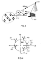
- the figure 3 illustrates an application to direction finding in the presence of multipaths.
- the m -th source 301 propagates along paths P 311, 312, 313 incidences ⁇ mp (1 ⁇ p ⁇ P) which are caused by P -1 obstacles 320 in the radio environment.
- the problem addressed in the method according to the invention is, in particular, to perform a 2D direction finding for coherent paths where the deviation of propagation time between the direct path and a secondary path is very small.
- the algorithms for handling the case of coherent sources are the Maximum Likelihood algorithms [2] [3] that are applicable on any geometric sensor networks.
- these techniques require the calculation of a multidimensional criterion whose number of dimensions depends on the number of paths and the number of incidence parameters per path. More particularly in the presence of K paths, the criterion is 2 K dimensions for a 2D direction finding to jointly estimate all the incidences ( ⁇ 1 , ..., ⁇ K ) . It should be noted that even in the presence of a number K 'of coherent paths less than the total number K of paths, the calculation of the maximum likelihood criterion remains at 2 K dimensions.
- the first determined component w of the wave vectors is the projection, on the axis formed by the linear sub-network, of the projection of the wave vectors on the formed plane. by the sensor network.
- w p cos ( ⁇ p - ⁇ ).
- the direction finding algorithm used to determine the second component is the maximum likelihood algorithm.
- the network is disturbed by mutual coupling of known matrix Z
- the method comprises a coupling suppression step executed before the estimation steps of the values of the components w and u, said coupling removal step determining a noise-cleaned covariance matrix by applying the following processing to the covariance matrix: Z -1 (R x - ⁇ 2
- x n (t) is the signal at the output of the nth sensor
- N the number of sensors
- n ( t ) is the additive noise
- ⁇ is the azimuth
- elevation and ⁇ ⁇ mp, mp ⁇ , ⁇ mp are respectively the attenuation, the direction and the p th delay paths of the m -th source.
- Z is the coupling matrix
- ⁇ is the wavelength
- ( u, v ) are the coordinates of the wave vector in the plane of the antenna.
- a ( ⁇ m , ⁇ m , P m ) is the response of the sensor array to the mth source
- ⁇ m [ ⁇ m 1 ⁇ ⁇ mP ' m ] T
- ⁇ m [ ⁇ m 1 ⁇ ⁇ mP m ] T.
- the source vector of the source is no longer a ( ⁇ m 1 ) but a composite director vector a ( ⁇ m , ⁇ m , P m ) dependent on a larger number of parameters.
- a first MUSIC-coherent algorithm [4] is first presented.
- the expression of the matrix R x is the following from (4):
- R x AR s ⁇ AT H + ⁇ 2 ⁇ I NOT with ⁇
- the rank of the matrix R x is K.
- the NK eigenvectors e i ( K +1 ⁇ l ⁇ N ) associated with the lowest eigenvalues of R x are orthogonal to the vectors e k (1 k k ⁇ K ) of the expression (6) and define the noise space . Since the vectors e i and e k are orthogonal, the direction vectors a ( ⁇ ⁇ , ⁇ ⁇ , K i ) are orthogonal to the noise vectors e i .
- the coherent MUSIC method described in [4] aims to reduce the number of search parameters of the MUSIC criterion.
- J MUSIC - Coherent ⁇ det D ⁇ ⁇ H ⁇ b ⁇ D ⁇ det D ⁇ ⁇ H D ⁇
- det ( M ) is the determinant of matrix M.
- the MUSIC-coherent criterion remains four-dimensional for azimuth-elevation goniometry. More generally, the MUSIC-coherent method requires the calculation of a criterion (9) having 2 K max dimensions. However, the method makes no assumption on the geometry of the network because it does not require any constraint on the expression of the director vector a ( ⁇ ).
- R x E [ x ( t ) x ( t ) H ].
- This procedure aims to obtain a matrix R x SM having a rank higher than the R x i without destroying the structure of the signal space generated by A 1 .
- Spatial smoothing and Forward-Backward techniques can be combined to increase decorrelation capacity in number of trips. These smoothing techniques make it possible to process the coherent sources with computing power very close to the implementation of a single direction finding algorithm such as MUSIC.
- the figure 6 shows that a network composed of two sub-networks 601, 602 of four sensors contains at least seven sensors.
- This network also has the disadvantage of being weakly open (or has a small footprint space) because the four-sensor subnetworks must be unambiguous. Since the sub-networks are composed of four sensors, this ambiguity constraint requires an inter-sensor spacing of less than ⁇ / 2. Indeed, the more open a network is, the more accurate the arrival angles are estimated with a better robustness to calibration errors. In the case where it is desired to perform an azimuth goniometry only, the constraint C3 is no longer present and the network making it possible to perform a direction finding on two coherent sources composed of two subareas of four sensors is a linear network equi -space with five sensors.
- Each sub-network is then a linear network equi-spaced four sensors.
- the figure 7 shows that the linear subnetwork 701 which allows azimuth direction finding two coherent paths has the following differences with respect to the network 702 which makes it possible in azimuth-elevation: on the one hand, it is composed of fewer sensors: five instead of seven, on the other hand, it has a larger footprint: 4d instead of 3d knowing that d is a distance less than ⁇ / 2, where ⁇ is the wavelength of the transmitted signals.
- the decorrelation of two coherent paths for an azimuth-site direction finding requires a network of sensors having more sensors and less opening than the network making it possible to perform a direction finding in azimuth only.
- a linear network that is not necessarily equi-spaced is sufficient.
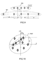
- the figure 9 shows that the Forward-Backward technique makes it possible, compared to the spatial smoothing technique, to perform unambiguous direction finding on two paths coherent with a network 901 having a larger aperture (10d instead of 4d for a network 902 used for spatial smoothing).
- the Forward-Backward technique has the advantage of not imposing a geometry constraint on half of the network. The other half of the network is symmetrical to the first half.
- the method according to the invention presented mixes the MUSIC method consistent with a Forward-Backward technique and / or spatial smoothing.
- the method contemplates using a sensor array containing a linear subnetwork on which a spatial and / or forward smoothing technique.
- -Backward is possible.
- the figure 10 shows such a network 1001 with a linear subnet 1002 having an orientation ⁇ with respect to the x-axis.
- the preceding steps show that the computation of a 2 K max dimension criterion for the MUSIC-coherent algorithm alone in 2D has been replaced by the computation of a MUSIC criterion with one dimension according to the parameter w and the cost of computation of the MUSIC-coherent criterion in 1 D with the variable u having K max dimensions.
- nb is large by being proportional to the size of the network ( nb > 50).
- u k is a consistent parameter vector for MUSIC when J MUSIC - Coherent u k ⁇ ⁇ K max where ⁇ (K max ) is a threshold between 0 and 1 because the criterion J MUSIC-Coherent ( u ) is normalized.
- ⁇ is a threshold between 0 and 1 because the criterion J MUSIC ( w ) is normalized.
- step B of the process can be applied several times.
- ⁇ i ⁇ ⁇ X i for 1 ⁇ i ⁇
- the number L as well as the sets ⁇ i can be determined by a conventional arithmetic process.
- An advantage of the method according to the invention is that the minimum number of sensors for estimating the direction of arrival of K coherent paths in 2D is lower than with prior art methods, which require a number of sensors greater than 2 (K + 1), the method according to the invention requires only a number of sensors greater than K.
- Another advantage of the method according to the invention is that it makes it possible to estimate directions of arrival of the 2D paths with larger networks, which improves the accuracy of the estimation.
Description
La présente invention concerne un procédé de détermination des angles d'arrivée en azimut et en élévation de sources cohérentes. Elle est utilisée, par exemple, dans tous les systèmes de localisation dans un contexte urbain où le canal de propagation est perturbé par un grand nombre d'obstacles comme les immeubles. De manière générale, elle peut être utilisée pour localiser des émetteurs, par exemple un téléphone portable, dans un contexte de propagation difficile, qu'il s'agisse d'un milieu urbain, semi-urbain — par exemple un site aéroportuaire —, de l'intérieur d'un bâtiment ou sous la neige, en cas d'avalanche. L'invention peut aussi être utilisée dans des procédés d'imagerie médicale, pour localiser des tumeurs ou des foyers épileptiques, les tissus du corps humain étant à l'origine de multi-trajets d'onde. Elle s'applique également dans des systèmes de sondage pour la recherche minière et pétrolière dans le domaine sismique, où l'on cherche à estimer des angles d'arrivées avec des multi-trajets dans le milieu de propagation complexe de la croûte terrestre.The present invention relates to a method for determining azimuth and elevation angles of arrival of coherent sources. It is used, for example, in all location systems in an urban context where the propagation channel is disturbed by a large number of obstacles such as buildings. In general, it can be used to locate transmitters, for example a mobile phone, in a context of difficult propagation, be it an urban, semi-urban environment - for example an airport site - inside a building or under the snow, in case of avalanche. The invention can also be used in medical imaging methods, for locating tumors or epileptic foci, the tissues of the human body being at the origin of multi-wave paths. It is also applicable in sounding systems for mining and oil exploration in the seismic field, where it is sought to estimate arrival angles with multipaths in the complex propagation medium of the earth's crust.
L'invention se situe dans le domaine technique du traitement d'antennes qui traite les signaux de plusieurs sources émettrices à partir d'un système de réception multi-capteurs. Plus particulièrement, l'invention concerne le domaine de la goniométrie qui consiste à estimer les angles d'arrivées des sources.The invention lies in the technical field of antenna processing which processes the signals of several emitting sources from a multi-sensor reception system. More particularly, the invention relates to the field of direction finding which consists in estimating the arrival angles of the sources.
Dans un contexte électromagnétique, les capteurs sont des antennes et les sources radioélectriques se propagent suivant une polarisation dépendante de l'antenne d'émission. Dans un contexte acoustique les capteurs sont des microphones et les sources sont sonores.In an electromagnetic context, the sensors are antennas and the radio sources propagate according to a polarization dependent on the transmitting antenna. In an acoustic context the sensors are microphones and the sources are sound.
La
D'après la
Les techniques de traitement d'antennes ont notamment pour objectif d'exploiter la diversité spatiale générée par la réception multi-antennes des signaux incidents, autrement dit, utiliser la position des antennes du réseau pour mieux utiliser les différences en incidence et distance des sources.Antenna processing techniques are intended in particular to exploit the spatial diversity generated by the multi-antenna reception of the incident signals, in other words, to use the position of the antennas of the network to make better use of the differences in incidence and distance of the sources.
La
Une méthode connue pour faire de la goniométrie est l'algorithme MUSIC [1]. Or, cet algorithme ne permet pas d'estimer les incidences des sources en présence de trajets cohérents.One known method for conducting direction finding is the MUSIC algorithm [1]. However, this algorithm does not make it possible to estimate the effects of the sources in the presence of coherent paths.
Les algorithmes permettant de traiter le cas des sources cohérentes sont les algorithmes du Maximum de Vraisemblance [2][3] qui sont applicables sur des réseaux de capteurs à géométrie quelconques. Toutefois ces techniques nécessitent le calcul d'un critère multidimensionnel dont le nombre de dimensions dépend du nombre de trajets ainsi que du nombre de paramètres d'incidence par trajet. Plus particulièrement en présence de K trajets, le critère est à 2K dimensions pour une goniométrie 2D afin d'estimer conjointement toutes les incidences (Θ 1 ,..., Θ K ). Il faut remarquer que même en présence d'un nombre K' de trajets cohérents inférieur au nombre total K de trajets, le calcul du critère du maximum de vraisemblance reste à 2K dimensions. Afin de réduire le nombre de dimensions du critère à 2K', une alternative est d'appliquer la méthode MUSIC-cohérent [4]. Toutefois, l'algorithme MUSIC-cohérent [4] nécessite un nombre de capteurs élevé et des ressources de calculs très importantes.The algorithms for handling the case of coherent sources are the Maximum Likelihood algorithms [2] [3] that are applicable on any geometric sensor networks. However, these techniques require the calculation of a multidimensional criterion whose number of dimensions depends on the number of paths and the number of incidence parameters per path. More particularly in the presence of K paths, the criterion is 2 K dimensions for a 2D direction finding to jointly estimate all the incidences ( Θ 1 , ..., Θ K ) . It should be noted that even in the presence of a number K 'of coherent paths less than the total number K of paths, the calculation of the maximum likelihood criterion remains at 2 K dimensions. In order to reduce the number of dimensions of the criterion to 2 K ', an alternative is to apply the MUSIC-coherent method [4]. However, the MUSIC-coherent algorithm [4] requires a high number of sensors and very important calculation resources.
Une autre alternative pour réduire le coût de calcul est de mettre en oeuvre des techniques de lissage spatial ou de Forward-Backward [5][6] (« Forward-Backward » signifiant passage avant - passage arrière), ces techniques nécessitant des géométries particulières de réseau. En effet, le lissage spatial est applicable lorsque le réseau se décompose en sous réseaux ayant la même géométrie (ex : Réseau linéaire équi-espacé ou réseau sur une grille 2D régulière). L'algorithme du Forward-Backward nécessite un réseau avec un centre de symétrie. Ces techniques d'avèrent très contraignantes en terme de géométrie du réseau de capteurs, a fortiori pour une goniométrie 2D, où la contrainte de symétrie ou de sous-réseaux identiques translatés est difficile à satisfaire.Another alternative to reduce the cost of calculation is to use techniques of spatial smoothing or Forward-Backward [5] [6] ("Forward-Backward"), these techniques requiring particular geometries network. Indeed, spatial smoothing is applicable when the network is broken down into subnetworks having the same geometry (ex: Equi-spaced linear network or network on a regular 2D grid). The Forward-Backward algorithm requires a network with a center of symmetry. These techniques prove to be very restrictive in terms of geometry of the sensor array, especially for a 2D direction finding, where the symmetry constraint or identical translated subnets is difficult to satisfy.
Pour la goniométrie en 1 D, des techniques de lissage spatial ont été envisagées sur des réseaux quelconques[6][7]. Pour ce faire, le réseau de capteurs est interpolé suivant la géométrie adaptée au lissage spatial (ou Forward-Backward). Dans [6] la technique d'interpolation ne s'intéresse qu'à un seul secteur angulaire et dans [7] l'algorithme est adapté aux cas de plusieurs secteurs angulaires pour l'interpolation. Toutefois ce genre de technique est difficilement adaptable au cas de la goniométrie 2D.For 1 D direction finding, spatial smoothing techniques have been proposed for any networks [6] [7]. To do this, the sensor array is interpolated according to the geometry adapted to the spatial smoothing (or Forward-Backward). In [6] the interpolation technique is only interested in one angular sector and in [7] the algorithm is adapted to the case of several angular sectors for the interpolation. However, this kind of technique is difficult to adapt to the case of 2D direction finding.
Un but de l'invention est de proposer une méthode pour déterminer, à partir d'un réseau de capteurs, la direction d'arrivée en azimut et en élévation de signaux cohérents avec un coût de calcul réduit et en limitant le plus possible les contraintes géométriques à imposer au réseau de capteurs. A cet effet, l'invention a pour objet un procédé de détermination conjointe de l'angle d'azimut θ et de l'angle d'élévation Δ des vecteurs d'ondes de P ondes dans un système comprenant un réseau de capteurs, plusieurs ondes parmi les P ondes se propageant selon des trajets cohérents ou sensiblement cohérents entre une source et lesdits capteurs, le procédé étant caractérisé en ce qu'il comprend au moins les étapes suivantes :
- ■ sélectionner un sous-ensemble de capteurs parmi les dits capteurs pour former un sous-réseau linéaire de capteurs ;
- ■ appliquer, sur les signaux issus du sous-réseau choisi, un algorithme suivant une seule dimension pour décorréler les sources des P ondes ;
- ■ déterminer une première composante w desdits vecteurs d'onde en appliquant, sur les signaux observés sur les capteurs du sous-réseau choisi, un algorithme de goniométrie suivant la seule dimension w ;
- ■ déterminer une deuxième composante u desdits vecteurs d'onde en appliquant un algorithme de goniométrie suivant la seule dimension u sur les signaux issus de l'ensemble du réseau de capteurs,
- ■ déterminer θ et Δ à partir de w et u.
- ■ select a subset of sensors from said sensors to form a linear subnet of sensors;
- ■ apply, on the signals coming from the chosen sub-network, a one-dimensional algorithm to decorrelate the sources of the waves;
- Determining a first component w of said wave vectors by applying, on the signals observed on the sensors of the chosen sub-network, a goniometry algorithm according to the single dimension w;
- Determining a second component u of said wave vectors by applying a goniometry algorithm based on the single dimension u on the signals coming from the entire sensor network,
- ■ determine θ and Δ from w and u.
Selon une mise en oeuvre du procédé selon l'invention,
- ■ on choisit les capteurs constituant le sous-réseau de telle sorte qu'au moins une partie du sous-réseau soit invariante par translation ;
- ■ on applique un algorithme de lissage spatial pour décorréler les sources des P ondes.
- The sensors constituting the sub-network are chosen so that at least part of the sub-network is invariant by translation;
- A spatial smoothing algorithm is applied to decorrelate the sources of the waves.
Selon une mise en oeuvre du procédé selon l'invention,
- ■ on choisit les capteurs constituant le sous-réseau de telle sorte qu'au moins une partie de sous-réseau comporte un centre de symétrie ;
- ■ on applique un algorithme de Forward-Backward pour décorréler les sources des P ondes.
- The sensors constituting the sub-network are chosen so that at least one part of the sub-network comprises a center of symmetry;
- ■ a Forward-Backward algorithm is applied to decorrelate the sources of the waves.
Selon une mise en oeuvre du procédé selon l'invention, la première composante w déterminée des vecteurs d'onde est la projection, sur l'axe formé par le sous-réseau linéaire, de la projection des vecteurs d'onde sur le plan formé par le réseau de capteurs. Autrement dit, pour chaque trajet p, wp=cos(θp-α).cos(Δp), α étant l'angle en azimut selon lequel l'axe formé par le sous-réseau linéaire est orienté.According to an implementation of the method according to the invention, the first determined component w of the wave vectors is the projection, on the axis formed by the linear sub-network, of the projection of the wave vectors on the formed plane. by the sensor network. In other words, for each path p, w p = cos (θ p -α). Cos (Δ p ), where α is the azimuth angle in which the axis formed by the linear subarray is oriented.
Selon une mise en oeuvre du procédé selon l'invention, le procédé comporte au moins les étapes suivantes :
- ■ calculer la matrice de covariance Rx sur l'ensemble du réseau de capteurs ;
- ■ extraire à partir de Rx, la matrice de covariance Rx' correspondant au sous-réseau linéaire choisi ;
- ■ appliquer un algorithme de décorrélation des sources sur Rx' ;
- ■ estimer, pour chaque trajet p, les valeurs de la première composante wp=cos(θp-α).cos(Δp) en appliquant un algorithme de goniométrie en 1 D sur la matrice Rx' décorrélée, α étant l'angle d'orientation en azimut de l'axe formé par le sous-réseau linéaire ;
- ■ estimer les valeurs de la deuxième composante up= cos(θp).cos(Δp), pour chaque trajet p, en appliquant un algorithme de goniométrie en 1 D sur la matrice Rx ;
- ■ déterminer, à partir des valeurs des couples (wp, up), les valeurs des couples azimut-élévation (θp, Δp).
- Compute the covariance matrix R x over the entire sensor network;
- Extracting from R x , the covariance matrix R x 'corresponding to the chosen linear subnetwork;
- ■ apply a source decorrelation algorithm on R x ';
- ■ estimate, for each path p, the values of the first component w p = cos (θ p -α) .cos (Δ p ) by applying a 1 D direction finding algorithm on the decorrelated matrix R x ', α being the azimuth orientation angle of the axis formed by the linear subnetwork;
- ■ estimate the values of the second component u p = cos (θ p ) .cos (Δ p ), for each path p, by applying a 1 D direction finding algorithm on the matrix R x ;
- ■ determine, from the values of the pairs (w p , u p ), the values of the azimuth-elevation pairs (θ p , Δ p ).
Selon une mise en oeuvre du procédé selon l'invention, l'algorithme de goniométrie utilisé pour déterminer la première composante w de chaque vecteur d'onde P est l'algorithme MUSIC, le critère JMUSIC à minimiser pour déterminer ladite composante w étant égal à 
où Π b l est le projecteur bruit extrait de la matrice de covariance décorrélée Rx' correspondant au sous-réseau linéaire choisi, et a(w)' représente la réponse du sous-réseau choisi aux ondes incidentes P.According to one implementation of the method according to the invention, the direction finding algorithm used to determine the first component w of each wave vector P is the MUSIC algorithm, the criterion J MUSIC to minimize to determine said component w being equal at
where Π b l is the noise projector extracted from the decorrelated covariance matrix R x 'corresponding to the chosen linear subnetwork, and a ( w )' represents the response of the selected subnetwork to the incident waves P.
Selon une mise en oeuvre du procédé selon l'invention, l'algorithme de goniométrie utilisé pour déterminer la deuxième composante u est l'algorithme MUSIC-cohérent en une seule dimension, le critère à minimiser étant : 
où Θ ={f 1(u 1) ··· f k 
where Θ = { f 1 ( u 1 ) ··· f k
Selon une autre mise en oeuvre du procédé selon l'invention, l'algorithme de goniométrie utilisé pour déterminer la deuxième composante est l'algorithme du maximum de vraisemblance.According to another implementation of the method according to the invention, the direction finding algorithm used to determine the second component is the maximum likelihood algorithm.
Selon une mise en oeuvre du procédé selon l'invention, le réseau est perturbé par du couplage mutuel de matrice Z connue, et le procédé comporte une étape de suppression du couplage exécutée préalablement aux étapes d'estimation des valeurs des composantes w et u, ladite étape de suppression du couplage déterminant une matrice de covariance nettoyée du bruit en appliquant le traitement suivant sur la matrice de covariance : Z-1(Rx -σ2|)Z-1H, σ2 étant le niveau de bruit estimé.According to one implementation of the method according to the invention, the network is disturbed by mutual coupling of known matrix Z, and the method comprises a coupling suppression step executed before the estimation steps of the values of the components w and u, said coupling removal step determining a noise-cleaned covariance matrix by applying the following processing to the covariance matrix: Z -1 (R x -σ 2 |) Z -1H , where σ 2 is the estimated noise level.
Selon une mise en oeuvre du procédé selon l'invention, la détermination des couples de valeurs (θp, Δp) à partir des valeurs de couples (wp, up) est effectuée comme suit : 
où 
or
D'autres caractéristiques apparaîtront à la lecture de la description détaillée donnée à titre d'exemple et non limitative qui suit faite en regard de dessins annexés qui représentent :
- la
figure 1 , un exemple de signaux émis par un émetteur et se propageant vers un réseau de capteurs, - la
figure 2 , la représentation de l'incidence d'une source sur un plan de capteurs, - la
figure 3 , une illustration de la propagation de signaux en multi-trajets, - la
figure 4 , un exemple de réseaux de capteurs de position (xn,yn), - la
figure 5 , un exemple de réseau de capteurs composé de deux sous-réseaux invariants par translation, - la
figure 6 , un exemple de réseau de capteurs composé de deux sous-réseaux permettant de décorréler deux trajets cohérents en azimut-élévation, - la
figure 7 , un réseau linéaire de capteurs où le lissage spatial permet de décorréler deux trajets cohérents en azimut, - la
figure 8 , un réseau de capteurs comportant un centre de symétrie en O, - la
figure 9 , deux réseaux linéaires à cinq capteurs, permettant de décorréler deux trajets cohérents en azimut pour, respectivement, le lissage spatial et le forward-backward, - la
figure 10 , un premier exemple de réseau de capteurs contenant un sous-réseau linéaire de capteurs et compatible du procédé selon l'invention, - la
figure 11 , un second exemple de réseau de capteurs contenant un sous-réseau linéaire de capteurs et compatible du procédé selon l'invention.
- the
figure 1 , an example of signals emitted by a transmitter and propagating towards a network of sensors, - the
figure 2 , the representation of the incidence of a source on a sensor plane, - the
figure 3 , an illustration of the propagation of multipath signals, - the
figure 4 , an example of position sensor networks (x n , y n ), - the
figure 5 , an example of a sensor network composed of two translation invariant subarrays, - the
figure 6 , an example of a sensor network composed of two sub-networks making it possible to decorrelate two coherent paths in azimuth-elevation, - the
figure 7 , a linear array of sensors where spatial smoothing makes it possible to decorrelate two coherent paths in azimuth, - the
figure 8 , a sensor array comprising a center of symmetry in O, - the
figure 9 , two linear networks with five sensors, for decorrelating two coherent paths in azimuth for, respectively, the spatial smoothing and the forward-backward, - the
figure 10 , a first example of a sensor array containing a linear array of sensors and compatible with the method according to the invention, - the
figure 11 , a second example of a sensor array containing a linear array of sensors and compatible with the method according to the invention.
Avant de détailler un exemple de mise en oeuvre du procédé selon l'invention, quelques rappels sur la modélisation du signal en sortie d'un réseau de capteurs sont donnés.Before detailing an example of implementation of the method according to the invention, some reminders on the modeling of the signal at the output of a sensor array are given.
En présence de M sources où la m-ième source contient Pm multi-trajets, le signal en sortie du réseau de capteurs s'écrit de la façon suivante : 
où xn (t) est le signal en sortie du n-ième capteur, N le nombre de capteurs, n(t) est le bruit additif, a(Θ) est la réponse du réseau de capteurs à une source de direction Θ=(θ,Δ), θ est l'azimut, Δ l'élévation et ρ mp , θ mp , τ mp sont respectivement l'atténuation, la direction et le retard du p-ième trajets de la m-ième source. Le vecteur a(Θ) qui s'appelle aussi vecteur directeur dépend des positions (xn, yn ) des capteurs 401, 402, 403, 404, 405 (voir 
Où Z est la matrice de couplage, λ est la longueur d'onde et (u,v) sont les coordonnées du vecteur d'onde dans le plan de l'antenne.
En présence de trajets cohérents où les retards des trajets vérifient τ m1 =...=τ mPm , le modèle de signal de l'équation (1) devient 
où a(Θ m,ρm,P m) est la réponse du réseau de capteurs à la m-ième source, Θ m=[Θ m1···Θ mP' m ] T et ρm=[ρ m1 ··· ρ mP
where x n (t) is the signal at the output of the nth sensor, N the number of sensors, n ( t ) is the additive noise, a ( Θ ) is the response of the sensor array to a source of direction Θ = (θ, Δ), θ is the azimuth, elevation and ρ Δ mp, mp θ, τ mp are respectively the attenuation, the direction and the p th delay paths of the m -th source. The vector a ( Θ ) which is also called director vector depends on the positions ( x n , y n ) of the
Where Z is the coupling matrix, λ is the wavelength and ( u, v ) are the coordinates of the wave vector in the plane of the antenna.
In the presence of coherent paths where the delays of the paths satisfy τ m 1 = ... = τ mPm , the signal model of equation (1) becomes
where a ( Θ m , ρ m , P m ) is the response of the sensor array to the mth source, Θ m = [ Θ m 1 ··· Θ mP ' m ] T and ρ m = [ρ m 1 ··· ρ mP
De façon plus générale, en présence de K groupes de trajets cohérents, le signal s'écrit : 
Pour permettre au lecteur de mieux comprendre le procédé selon l'invention, le traitement des sources cohérentes en azimut-élévation dans l'état de l'art est explicité ci-après.To allow the reader to better understand the method according to the invention, the treatment of coherent sources in azimuth-elevation in the state of the art is explained below.
Un premier algorithme MUSIC-cohérent [4] est d'abord présenté. L'algorithme MUSIC [1] est une méthode à haute résolution basée sur la décomposition en éléments propres de la matrice de covariance R x =E[x(t) x(t) H ] du signal multi-capteurs x(t), où E[.] est l'espérance mathématique. L'expression de la matrice R x est la suivante d'après (4) : 
En présence de K groupes de trajets cohérents, le rang de la matrice R x vaut K. Dans ces conditions les K vecteurs propres e k (1≤k≤K) associés aux K plus fortes valeurs propres λ k de R x vérifient 
Les N-K vecteurs propres e i (K +1 ≤ l ≤N) associés aux plus faibles valeurs propres de R x sont orthogonaux aux vecteurs e k (1≤k≤K) de l'expression (6) et définissent l'espace bruit. Comme les vecteurs e i et e k sont orthogonaux, les vecteurs directeurs a(Θ ¡ ,ρ ¡ ,Ki ) sont orthogonaux aux vecteurs bruit e i . Dans ces conditions, les K minima (Θ k, ρ k' Kk ) du critère suivant de MUSIC 
permettent de donner les directions Θ k de chaque trajet. Toutefois le coût de calcul du critère de l'équation (7) est très important car dépend de l'incidence de Kmax trajets cohérents ainsi que de leurs amplitudes relatives : (Θ,ρ).allow to give the directions Θ k of each path. However, the cost of calculating the criterion of equation (7) is very important because it depends on the incidence of K max coherent paths as well as their relative amplitudes: ( Θ , ρ).
La méthode MUSIC cohérent décrit dans [4] a pour objectif de réduire le nombre de paramètres de recherche du critère de MUSIC. Pour ce faire le vecteur a(Θ m,ρm,Pm ) de l'équation (3) se ré-écrit de la manière suivante : 
Dans ces conditions, le critère de l'équation (7) se réduit a l'expression suivante : 
Où det(M) est le déterminant de la matrice M. Le nombre de dimensions du critère est alors réduit au 2Kmax paramètres de Θoù Kmax est le nombre maximum de trajets cohérents. En conséquence les K minima du critère JMUSIC-Coherent (Θ) donnent les directions Θ k = {Θ k1 ··· Θ kK
Where det ( M ) is the determinant of matrix M. The number of dimensions of the criterion is then reduced to the 2K max parameters of Θ where K max is the maximum number of coherent paths. Consequently the K minima of the J MUSIC-Coherent criterion ( Θ ) give the directions Θ k = { Θ k 1 ··· Θ kK
Des méthodes alternatives et également connues pour le traitement des sources cohérentes sont les techniques de lissage spatial [5][6] et de Forward-Backward [5]. Ces méthodes permettent de décorréler des sources en effectuant un simple pré-traitement sur la matrice de covariance des signaux reçus. Il est alors possible d'appliquer un algorithme de goniométrie tel que MUSIC sur la nouvelle matrice de covariance. Ces techniques sont issues du domaine de l'analyse spectrale dont l'objectif est de modéliser le spectre en fréquence d'un signal.Alternative and equally known methods for the treatment of coherent sources are spatial smoothing techniques [5] [6] and Forward-Backward [5]. These methods make it possible to decorrelate sources by performing a simple pre-treatment on the matrix of covariance of the received signals. It is then possible to apply a direction finding algorithm such as MUSIC on the new covariance matrix. These techniques come from the field of spectral analysis whose objective is to model the frequency spectrum of a signal.
Les techniques de lissage spatial [5][6] sont applicables sur un réseau de capteurs composé de sous-réseaux 501, 502 invariants par translation comme illustré sur la 
avec A=[a(Θ 1)... a(Θ P )].
L'expression du signal reçu sur le i-ième sous réseau s'écrit alors : 
où A i =[ a i (Θ 1)... a i (Θ P )], P i étant une matrice composée de 0 et de 1 permettant de sélectionner le signal du i-ième sous réseau dont le vecteur directeur a i (Θ) vérifie la relation suivante : ![]()
En rappelant que l'incidence Θ=(θ,Δ) dépend des deux paramètres θ et Δ.Spatial smoothing techniques [5] [6] are applicable on a sensor network composed of translation-
with A = [ a ( Θ 1 ) ... a ( Θ P )].
The expression of the signal received on the i-th subnet is then written:
where A i = [a i (Θ 1) ... a i (Θ P)], P i being a matrix composed of 0 and 1 for selecting the i-th subnetwork signal whose direction vector a i ( Θ ) check the following relation: ![]()
Reminding that the incidence Θ = (θ, Δ) depends on the two parameters θ and Δ.
D'après (11)(12), la matrice de mélange A i du i-ième sous réseau vérifie ![]()
![]()
D'après (11)(13) la matrice de covariance R x i =E[x(t) i x(t) iH ] a l'expression suivante : ![]()
![]()
En conséquence, une alternative des techniques de lissage spatial consiste à appliquer un algorithme de type MUSIC sur la matrice de covariance suivante : 
où R x =E[x(t) x(t) H ]. Cette procédure a pour objectif d'obtenir une matrice R x SM ayant un rang plus élevé que les R x i sans détruire la structure de l'espace signal engendré par A 1. En effet cette technique permet de décorréler au maximum / trajets cohérents car 
Et ainsi ![]()
![]()
La technique de lissage par Forward-Backward [5] nécessite un réseau de capteurs ayant un centre de symétrie en O comme indiqué dans la 
où selon la ![]()
Où Π est une matrice de permutation composée de 0 et 1. La technique de lissage par Forward-Backward consiste à appliquer un algorithme de goniométrie tel que MUSIC sur la matrice de covariance suivante ![]()
Sachant que ![]()
la technique permet de décorréler deux trajets cohérents car ![]()

where R x = E [ x ( t ) x ( t ) H ]. This procedure aims to obtain a matrix R x SM having a rank higher than the R x i without destroying the structure of the signal space generated by A 1 . Indeed, this technique makes it possible to decorrelate as much as possible / coherent paths because
And so ![]()
![]()
The Forward-Backward smoothing technique [5] requires a sensor array with a center of symmetry in O as indicated in the diagram.
where according to the ![]()
Where Π is a permutation matrix composed of 0 and 1. The Forward-Backward smoothing technique consists in applying a direction finding algorithm such as MUSIC on the following covariance matrix ![]()
Knowing that ![]()
the technique makes it possible to decorrelate two coherent paths because ![]()
Les techniques de lissage spatial et Forward-Backward peuvent se combiner pour accroître la capacité de décorrélation en nombre de trajets. Ces techniques de lissage permettent de traiter les sources cohérentes avec une puissance de calcul très voisine de la mise en oeuvre d'un seul algorithme de goniométrie tel que MUSIC.Spatial smoothing and Forward-Backward techniques can be combined to increase decorrelation capacity in number of trips. These smoothing techniques make it possible to process the coherent sources with computing power very close to the implementation of a single direction finding algorithm such as MUSIC.
Lorsque le réseau de capteur est perturbé par du couplage mutuel où le vecteur directeur s'écrit
![]()
![]()
![]()
![]()
En conséquence la matrice de covariance R x =E[x(t) x(t) H ] s'écrit de la manière suivante :
![]()
![]()
Sachant que  i = P i  =  1Φ i (où que Π Â* = ÂΦ FB ), les étapes suivantes permettent d'appliquer une technique de lissage spatial ou de Forward-Backward en présence de couplage mutuel :
- Etape n°L.1 : Décomposer en éléments propres la matrice de covariance R x =E[x(t) x(t) H ] tel que :

où E s et E b sont les matrices des vecteurs propres associés respectivement à l'espace signal et à l'espace bruit selon MUSICO et où Λ s et Λ b sont des matrices diagonales composées respectivement des valeurs propres de l'espace signal et des valeurs propres de l'espace bruit. - Etape n°L.2 : Extraire la matrice de covariance non bruitée Z(ÂR s  H )Z H en effectuant :

- Etape n°L.3 (Lissage spatial): Appliquer l'algorithme MUSIC sur la matrice de covariance R x SM suivante :

- Etape n°L.3 (Forward-Backward): Appliquer l'algorithme MUSIC sur la matrice de covariance R x FB suivante :

- Step n ° L.1: Decompose in eigen elements the covariance matrix R x = E [ x ( t ) x ( t ) H ] such that:
where E s and E b are the matrices of the eigenvectors respectively associated with the signal space and the noise space according to MUSICO and where Λ s and Λ b are diagonal matrices composed respectively of eigenvalues of the signal space and eigenvalues of the noise space. - Step L.2: Extract the noise-covariance matrix Z (s Ar-H) Z H by performing:
- Step # L.3 (Spatial Smoothing): Apply the MUSIC algorithm on the following covariance matrix R x SM :
- Step No. L.3 (Forward-Backward): Apply the MUSIC algorithm on the following covariance matrix R x FB :
Si le réseau de vecteur directeur â(Θ) le permet, les deux techniques de lissage des étapes n°L.3 peuvent être combinées.If the director vector array â ( Θ ) allows, both smoothing techniques of steps # L.3 can be combined.
Les techniques de lissage spatial sont applicables en présence de couplage mutuel. Toutefois cela impose des contraintes très fortes sur la géométrie du réseau élémentaire qui ont l'inconvénient de nécessiter un très grand nombre de capteurs. Dans l'exemple suivant nous allons évaluer le nombre minimal de capteurs pour traiter le cas de deux sources cohérentes en azimut-élévation. Pour cela il faut que :
- ■ contrainte C1 : Le nombre de capteurs de chaque sous-réseau soit au moins égal à Ni=4. En effet à cause des ambiguïtés, un réseau de N capteurs permet au plus d'estimer la direction d'arrivée de N/2 sources.
- ■ contrainte C2 : Le nombre de sous-réseaux soit au moins égal à 2.
- ■ contrainte C3 : Les sous-réseaux soient plan (non linéaires) afin de pouvoir effectuer une goniométrie en azimut-site.
- ■ C1 constraint: The number of sensors of each sub-network is at least equal to N i = 4. Indeed because of the ambiguities, a network of N sensors makes it possible at most to estimate the direction of arrival of N / 2 sources.
- ■ C2 constraint: The number of subnets is at least 2.
- ■ C3 constraint: The subnetworks are plane (non-linear) in order to be able to perform azimuth-site direction finding.
La
Pour le cas où l'on souhaiterait effectuer une goniométrie en azimut seulement, la contrainte C3 n'est plus présente et le réseau permettant d'effectuer une goniométrie sur deux sources cohérentes composé de deux sous-réseaux de quatre capteurs est un réseau linéaire équi-espacé à cinq capteurs. Chaque sous-réseau est alors un réseau linéaire équi-espacé à quatre capteurs. La
In the case where it is desired to perform an azimuth goniometry only, the constraint C3 is no longer present and the network making it possible to perform a direction finding on two coherent sources composed of two subareas of four sensors is a linear network equi -space with five sensors. Each sub-network is then a linear network equi-spaced four sensors. The
Pour la technique de Forward-Backward nécessitant un réseau avec un centre de symétrie comme illustré à la
La
Le procédé selon l'invention présenté mixe la méthode MUSIC cohérents à une technique de Forward-Backward et/ou de lissage spatial. Compte tenu des avantages et inconvénients des techniques de lissage et de l'algorithme MUSIC-cohérent décrits plus haut, le procédé envisage d'utiliser un réseau de capteurs contenant un sous-réseau linéaire sur lequel une technique de lissage spatial et/ou de Forward-Backward est envisageable. La
Les coordonnées (xn l, yn l ) du n-ième capteur du sous-réseau linéaire ont alors l'expression suivante : 
où Nl est le nombre de capteurs du sous-réseau linéaire. En l'absence de couplage et selon (2), le vecteur directeur a l (Θ) associé au sous-réseau linéaire s'écrit 
Le vecteur a l (Θ) dépend alors d'un seul paramètre w=cos(θ-α)cos(Δ) de la manière suivante : 
on note par x l (t) le signal en sortie du sous-réseau linéaire et part P roj la matrice composée de 0 et 1 permettant d'extraire les signaux du sous-réseau linéaire tel que ![]()
où x(t) est le signal observé sur tous les capteurs du réseau. La relation entre la variable w=cos(θ-α)cos(Δ) et les coordonnées du vecteur d'onde (u,v) de l'équation (2) est la suivante : ![]()
Connaissant w, l'incidence Θ devient une fonction 1 D dépendant du paramètre u tel que : 
où la fonction f(u, v) est donnée par l'expression (2). Lorsque α=0, le vecteur de paramètre Θ ne peut pas dépendre de la variable u : Dans ce cas, l'incidence Θ dépend la variable v avec la fonction Θ(v) =f((w-vsin(α))/cos(α),v). Pour des raisons de simplicité dans la description du procédé et sans nuire à la généralité, on supposera qu'il est toujours possible d'écrire Θ en fonction de u. En conséquence, 
where N l is the number of sensors in the linear subnetwork. In the absence of coupling and according to (2), the direction vector a I (Θ) associated with the linear subarray can be written as
The vector a l ( Θ ) then depends on a single parameter w = cos (θ-α) cos (Δ) as follows:
we denote by x l ( t ) the output signal of the linear sub-network and start from P roj the matrix composed of 0 and 1 allowing to extract the signals from the linear subnetwork such that ![]()
where x ( t ) is the signal observed on all sensors in the network. The relation between the variable w = cos (θ-α) cos (Δ) and the coordinates of the wave vector ( u, v ) of equation (2) is as follows: ![]()
Knowing w , the incidence Θ becomes a function 1 D depending on the parameter u such that:
where the function f ( u, v ) is given by the expression (2). When α = 0, the parameter vector Θ can not depend on the variable u : In this case, the incidence Θ depends on the variable v with the function Θ ( v ) = f (( w - v sin (α)) / cos (α), v ). For the sake of simplicity in the description of the process and without detracting from the generality, it will be assumed that it is always possible to write Θ as a function of u . Consequently,
En présence de P trajets dont au moins un groupe de Kmax sont cohérents, l'exemple présenté du procédé selon l'invention contient au minimum les étapes suivantes :
- ■ Etape A : Application d'une technique de lissage spatial et/ou de Forward-Backward sur le vecteur observation x i (t) du réseau linéaire. Après une goniométrie 1 D suivant la variable w, on obtient les paramètres d'incidences wp =cos(θ p -α)cos(Δ p ) pour (1≤p≤P). Le critère 1 D de MUSIC a l'expression suivante :

où Π b l est le projecteur bruit extrait de la matrice de covariance lissée. - ■ Etape B : En présence de Kmax ≤P trajets cohérents, application de la méthode MUSIC-cohérent décrite plus haut avec la variable Θ={Θ 1 ··· Θ K
max } qui est la fonction suivante de la variable u ={u 1 ··· u Kmax }
où le critère de MUSIC-cohérent JMUSIC-Coherent est une fonction de la variable u ayant Kmax dimensions. - ■ Etape C : à partir de K (K étant le rang de la matrice de covariance Rx) solutions u k minimisant la fonction JMUSIC-Coherent (u), il est possible d'extraire les P couples d'incidences (wp ,up ) pour (1≤p≤P) et d'en déduire les incidences (θ p, Δ p ) en effectuant

- Step A: Application of a spatial smoothing and / or Forward-Backward technique on the observation vector x i ( t ) of the linear network. After a 1 D direction finding according to the variable w , we obtain the parameters of incidence w p = cos (θ p -α) cos (Δ p ) for (1 ≤ p ≤ P ). The criterion 1 D of MUSIC has the following expression:
where Π b l is the noise projector extracted from the smoothed covariance matrix. - ■ Step B: In the presence of K max ≤ P coherent paths, application of the MUSIC-coherent method described above with the variable Θ = { Θ 1 ··· Θ K
max } which is the next function of the variable u = { u 1 ··· u Kmax }
where the criterion of MUSIC-coherent J MUSIC-Coherent is a function of the variable u having K max dimensions. - Step C: starting from K (K being the rank of the covariance matrix R x ) solutions u k minimizing the function J MUSIC-Coherent ( u ), it is possible to extract the P couples of incidences ( w p , u p ) for (1 ≤ p ≤ P ) and to deduce the incidences (θ p , Δ p ) by performing
Les étapes précédentes montrent que le calcul d'un critère à 2Kmax dimensions pour l'algorithme MUSIC-cohérent seul en 2D a été remplacé par le calcul d'un critère MUSIC à une dimension suivant le paramètre w et le coût de calcul du critère MUSIC-cohérent en 1 D avec la variable u ayant Kmax dimensions. Le gain en puissance de calcul est alors égal à 
où nb est le nombre de points des maillages des critères (MUSIC ou MUSIC-cohérent) suivant les variables u et v des composantes du vecteur d'onde. Dans le cas général nb est grand en étant proportionnel à la taille du réseau (nb>50).The preceding steps show that the computation of a 2 K max dimension criterion for the MUSIC-coherent algorithm alone in 2D has been replaced by the computation of a MUSIC criterion with one dimension according to the parameter w and the cost of computation of the MUSIC-coherent criterion in 1 D with the variable u having K max dimensions. The computing power gain is then equal to
where nb is the number of points of the meshes of the criteria (MUSIC or MUSIC-coherent) according to the variables u and v of the components of the wave vector. In the general case nb is large by being proportional to the size of the network ( nb > 50).
On considérera que u k est un vecteur de paramètre solution pour MUSIC cohérent lorsque ![]()
où η(Kmax) est un seuil compris entre 0 et 1 car le critère JMUSIC-Coherent ( u ) est normalisé. Lorsque le nombre K' de solutions u k est inférieur est inférieur au rang K de la matrice de covariance Rx on en déduit que le nombre de trajets cohérents est supérieur à Kmax. Pour le cas où K'< Kmax l'algorithme MUSIC cohérent sera appliqué avec Kmax = Kmax +1. En conséquence le procédé permet d'estimer conjointement les incidences des trajets avec le nombre de trajets cohérents.It will be considered that u k is a consistent parameter vector for MUSIC when ![]()
where η (K max ) is a threshold between 0 and 1 because the criterion J MUSIC-Coherent ( u ) is normalized. When the number K 'of solutions u k is smaller than the rank K of the covariance matrix R x, we deduce that the number of coherent paths is greater than K max . For the case where K '< K max the coherent MUSIC algorithm will be applied with K max = K max +1 . Consequently, the method makes it possible to jointly estimate the incidences of the paths with the number of coherent paths.
De la même manière on considérera que wp est un paramètre solution de la goniométrie 1 D de l'étape A lorsque ![]()
![]()
Où η est un seuil compris entre 0 et 1 car le critère JMUSIC (w) est normalisé.Where η is a threshold between 0 and 1 because the criterion J MUSIC ( w ) is normalized.
Le procédé envisage de traiter le cas où au moins deux trajets cohérents vérifient wi =wj avec ui ≠ uj. Ce problème est détectable lorsque :
- ■ le rang de la matrice de covariance lissé reste égal à celui de la matrice de covariance Rx ;
- ■ la méthode MUSIC ne fonctionne pas sur la matrice de covariance non lissée Rx.
- The rank of the smoothed covariance matrix remains equal to that of the covariance matrix R x ;
- ■ the MUSIC method does not work on the unsmoothed covariance matrix Rx.
En supposant qu'il existe Kmax trajets cohérents et que MUSIC 1 D en w donne P'< Kmax solutions de trajets cohérents, la méthode consiste à compléter la liste incomplète de P' éléments {wp } par Kmax -P' estimation de la liste initiale des {wp }. Plus précisément en présence de Kmax=2 trajets cohérents et P'=1 paramètre w 1 détecté, il faut appliquer la méthode MUSIC-cohérent de l'étape B avec w 1=w 1 et w 2= w 1 soit l'ensemble de paramètres { w 1, w 1}. Dans le cas où Kmax =3 trajets cohérents et P'=2 , il existe deux configurations sur lesquelles l'étape B de MUSIC-cohérent en 1 D doit être appliqué: {w 1, w 2, w 2} et {w 1 , w 1 , w 2}. En conséquence lorsque P'< Kmax l'étape B du procédé peut-être appliquée plusieurs fois. Il existe ainsi L ensembles d'incidences wp suivants sur lesquelles l'étape B du procédé doit être appliqué : 
Le nombre L ainsi que les ensembles Ω i peuvent être déterminés par un processus classique d'arithmétique.Assuming that there are K max coherent paths and that MUSIC 1 D in w gives P '<K max coherent path solutions, the method consists in completing the incomplete list of P ' elements { w p } by K max - P ' estimate of the initial list of { w p }. More precisely in the presence of K max = 2 coherent paths and P '= 1 parameter w 1 detected, it is necessary to apply the MUSIC-coherent method of step B with w 1 = w 1 and w 2 = w 1 is all of parameters { w 1 , w 1 }. In the case where K max = 3 coherent paths and P '= 2, there are two configurations on which the MUSIC-coherent step B in 1 D must be applied: { w 1 , w 2 , w 2 } and { w 1 , w 1 , w 2 }. Consequently, when P '<K max, step B of the process can be applied several times. There are thus L following implications w p sets on which step B of the process is to be applied:
The number L as well as the sets Ω i can be determined by a conventional arithmetic process.
Les étapes suivantes du procédé permettent d'estimer la direction d'arrivée de P trajets en azimut-élévation sachant qu'il existe au moins un groupe de Kmax trajets cohérents et que le réseau est perturbé par du couplage mutuel de matrice Z connu.
- Etape n°1 : Décomposition en éléments propres de la matrice de covariance R x =E[x(t) x(t) H ] tel que

où E est la matrice des vecteurs propres et Λ est une matrice diagonale composée des valeurs propres. - Etape n°2: A partir des valeurs propres de la matrice Λ détermination du nombre K de valeurs propres dominantes donnant le rang de R x .
- Etape n°3 : Décomposition suivante de la matrice R x

Où E s et E b sont les matrices des vecteurs propres associés respectivement à l'espace signal sachant que dim(E s )=NxK et où ∧ s et λ b sont des matrices diagonales composées respectivement des valeurs propres de l'espace signal et des valeurs propres de l'espace bruit. - Etape n°4 : Extraction de la matrice de covariance non bruitée et sans couplage en effectuant

Où K est la dimension de l'espace signal tel que K≤P. - Etape n°5 : Calcul du projecteur bruit de la matrice R y de la manière suivante :

- Etape n°6: Application de l'algorithme MUSIC en 2D avec le critère JMUSIC (Θ)=(Θ) H Π b H
 (Θ)/(Θ) H(Θ)) avec le vecteur(Θ) de l'équation (22). Estimation de P 0≤K incidences Θ p (1≤p≤ P 0) vérifiant JMUSIC(Θ p )<η(1). Formation de l'ensemble Θ={Θ 1 ... Θ P0 } des trajets non-cohérents. Si P 0<K aller à l'étape n°7.
 - Etape n°7 : Calcul de la matrice de covariance du réseau linéaire en effectuant R x l = P roj Rx P roj H sachant que x l (t) = P roj x(t).
- Etape n°8 : Application d'une (ou des deux) technique(s) de lissage sur la matrice R x l du réseau linéaire en effectuant soit

- Etape n°9 : A partir d'une décomposition en élément propre de la matrice R̃ x estimation du rang P de l'espace signal ainsi que du projecteur bruit Π b l =E b E b H (Etape de l'algorithme MUSIC rappelé dans les étapes 1 à 3 de ce procédé pour la matrice R x).
- Etape n°10 : Application de l'algorithme MUSIC en 1 D avec le critère JMUSIC (w)=(a l (w) H Π b l a l (w))/(a l (w) H a l (w)) avec le vecteu a l (w) de l'équation (28). Estimation de P incidences wp (1≤p≤ P) vérifiant JMUSIC (wp )<η.
- Etape n°11 : Formation de l'ensemble Ψ des incidences wp associé à un trajet cohérent tel que Ψ={ wp ≠cos(θi -α)cos(Δ i ) où Θ i ={θ i ,Δ i }∈Θ}
- Etape n°12 : Si P>K alors Kmax =cardinal(Ψ) et L=1 avec Ω1=Ψ. Aller à l'étape n°14.
- Etape n°13 : Si P≤K alors Kmax=K+1 et constitution des L ensembles de paramètres Ωi de l'équation (39) avec P'= cardinal(Ψ).
- Etape n°14 : i=1
- Etape n°15 : Application des étapes B et C de MUSIC cohérent 1 D décrit à la page 18 avec Θ =f( u )={f 1(u 1)···f K
max (uKmax )} sachant que fp (u)=f(u,(wp-u cos(α))/sin(α)) où wp ∈Ω i . Obtention de Ki incidences Θ k pour (1≤k≤Ki ). - Etape n°16 : Pour k allant de 1 à Ki si Θ k∉Θ alors Θ=Θ∪{Θ k }
- Etape n°17 : i= i +1. Si i ≤ L alors retour à l'étape n°14.
- Step n ° 1: Decomposition in eigen elements of the covariance matrix R x = E [ x ( t ) x ( t ) H ] such that
where E is the matrix of eigenvectors and Λ is a diagonal matrix composed of eigenvalues. - Step 2: From the eigenvalues of the matrix Λ determination of the number K of dominant eigenvalues giving the rank of R x .
- Step 3: Next decomposition of the matrix R x
Where E s and E b are the matrices of the eigenvectors associated respectively with the signal space knowing that dim ( E s ) = N x K and where ∧ s and λ b are diagonal matrices composed respectively of the eigenvalues of the space signal and eigenvalues of the noise space. - Step 4: Extraction of the unmisted and unmatched covariance matrix by performing
Where K is the signal space dimension such that K ≤ P. - Step 5: Calculation of the projector noise of the matrix R y as follows:
- Step 6: Application of the MUSIC algorithm in 2D with the criterion J MUSIC ( Θ ) = ( Θ ) H Π b H( Θ ) / (Θ ) H( Θ )) with the vector( Θ ) of equation (22). Estimation of P 0 ≤ K incidences Θ p (1 ≤ p ≤ P 0 ) satisfying J MUSIC ( Θ p ) <η (1). Formation of the set Θ = { Θ 1 ... Θ P0 } of non-coherent paths. If P 0 < K go to step # 7.
- Step 7: Calculation of the covariance matrix of the linear array by performing the R x = R x P P roj roj H where x l (t) = P roj x (t).
- Step 8: Application of one or both smoothing techniques to the linear network matrix R x 1 by performing either
- Step n ° 9: From a decomposition into an own element of the matrix R x estimation of the rank P of the signal space as well as the projector noise Π b l = E b E b H (Step of the MUSIC algorithm recalled in
steps 1 to 3 of this method for the matrix R x ). - Step n ° 10: Application of the MUSIC algorithm in 1 D with the criterion J MUSIC ( w ) = ( a l ( w ) H Π b l a l ( w )) / ( a l ( w ) H a l ( w )) with the vecteu at l ( w ) of equation (28). Estimation of P incidences w p (1 ≤ p ≤ P ) satisfying J MUSIC ( w p ) < η.
- Step n ° 11: Formation of the set Ψ of incidences w p associated with a coherent path such that Ψ = { w p ≠ cos ( θ i -α ) cos (Δ i ) where Θ i = {θ i , Δ i } ∈ Θ }
- Step # 12: If P > K then K max = cardinal (Ψ) and L = 1 with Ω 1 = Ψ. Go to step # 14.
- Step n ° 13: If P ≤ K then K max = K +1 and constitution of L sets of parameters Ω i of equation (39) with P '= cardinal (Ψ).
- Step 14: i = 1
- Step 15: Application of steps B and C of MUSIC coherent 1 D described on page 18 with Θ = f ( u ) = { f 1 ( u 1 ) ··· f K
max ( u Kmax )} knowing that f p ( u ) = f ( u, ( w p -u cos (α)) / sin (α)) where w p ∈Ω i . Obtaining K i incidences Θ k for (1 k k ≤ K i ). - Step n ° 16: For k going from 1 to K i if Θ k ∉ Θ then Θ = Θ ∪ { Θ k }
- Step 17: i = i +1. If i ≤ L then return to step # 14.
Un avantage du procédé selon l'invention est que le nombre minimal de capteurs pour estimer la direction d'arrivée de K trajets cohérents en 2D est plus faible qu'avec des procédés de l'art antérieur, lesquels nécessitent un nombre de capteurs supérieur à 2(K+1), le procédé selon l'invention ne nécessitant qu'un nombre de capteurs supérieur à K.An advantage of the method according to the invention is that the minimum number of sensors for estimating the direction of arrival of K coherent paths in 2D is lower than with prior art methods, which require a number of sensors greater than 2 (K + 1), the method according to the invention requires only a number of sensors greater than K.
Un autre avantage du procédé selon l'invention est qu'il permet d'estimer des directions d'arrivée des trajets en 2D avec des réseaux plus grand, ce qui améliore la précision de l'estimation.Another advantage of the method according to the invention is that it makes it possible to estimate directions of arrival of the 2D paths with larger networks, which improves the accuracy of the estimation.
-
[1]
RO. SCHMIDT, Multiple emitter location and signal parameter estimation, in Proc of the RADC Spectrum Estimation Workshop, Griffiths Air Force Base, New York, 1979, pp. 243-258 RO. Schmidt, Multiple emitter location and signal parameter estimation, in Proc of the RADC Spectrum Estimation Workshop, Griffith Air Force Base, New York, 1979, pp. 243-258 -
[2]
P. Larzabal Application du Maximum de vraisemblance au traitement d'antenne : radio-goniométrie et poursuite de cibles. PhD Thesis, Université de Paris-sud, Orsay, FR, June 1992 P. Larzabal Maximum likelihood application to antenna processing: radio-direction finding and target tracking. PhD Thesis, University of Paris-Sud, Orsay, FR, June 1992 -
[3]
B.Ottersten, M.Viberg, P.Stoica and A.Nehorai, Exact and large sample maximum likelihood techniques for parameter estimation and detection in array processing. In S.Haykin, J.Litva and TJ.Shephers editors, Radar Array Processing, chapter 4, pages 99-151. Springer-Verlag, Berlin 1993 B.Ottersten, M.Viberg, P.Stoica and A.Nehorai, Exact and large sample. In S.Haykin, J.Litva and TJ.Shephers editors, Radar Array Processing, chapter 4, pages 99-151. Springer-Verlag, Berlin 1993 -
[4]
A.FERREOL, E.BOYER, et P.LARZABAL, « Low cost algorithm for some bearing estimation in presence of separable nuisance parameters», Electronic-Letters , IEE, vol 40 , n°15 , pp966-967 , july 2004 A. FERREOL, E. BOYER, and P. LARZABAL, "Low cost algorithm for some bearing estimation in the presence of separable nuisance parameters", Electronic-Letters, IEE, Vol 40, No. 15, pp966-967, July 2004 -
[5]
S. U. Pillai and B. H. Kwon, Forward/backward spatial smoothing techniques for coherent signal identification, IEEE Trans. Acoust., Speech and Signal Processing, vol. 37, pp. 8-15, Jan. 1988 SU Pillai and BH Kwon, Forward / backward spatial smoothing techniques for coherent signal identification, IEEE Trans. Acoust., Speech and Signal Processing, Vol. 37, pp. 8-15, Jan. 1988 -
[6]
B. Friedlander and A. J. Weiss. Direction Finding using spatial smoothing with interpolated arrays. IEEE Transactions on Aerospace and Electronic Systems, Vol. 28, No. 2, pp. 574-587, 1992 B. Friedlander and AJ Weiss. Direction Finding using spatial smoothing with interpolated arrays. IEEE Transactions on Aerospace and Electronic Systems, Vol. 28, No. 2, pp. 574-587, 1992 -
[7] A. Ferréol, J.Brugier et Ph.Morgand Procédé d'estimation des angles d'arrivées de sources cohérentes par une technique de lissage spatial sur un réseau de capteurs quelconque. Brevet publié sous le numéro
FR 2917180 FR 2917180
Claims (10)
- A method for jointly determining the angle of azimuth θ and the angle of elevation Δ of the wave vectors of P waves in a system comprising an array (1001) of sensors, several waves among the P waves propagating along coherent paths between a source and said sensors, said method being characterised in that it comprises at least the following steps:■ selecting a sub-set of sensors from said sensors so as to form a linear sub-array (1002) of sensors;■ applying, to the signals coming from the selected sub-array, a one dimension algorithm for decorrelating the sources of the P waves;■ determining a first component w of said wave vectors by applying a goniometry algorithm in one dimension w to the signals that are observed on the sensors of the selected sub-array;■ determining a second component u of said wave vectors by applying a goniometry algorithm in one dimension u to the signals coming from the entire array of sensors;■ determining θ and Δ from w and u.
- The method according to claim 1, characterised in that:■ the sensors that constitute the sub-array are selected so that at least one part of said sub-array is invariant by translation;■ a spatial smoothing algorithm is applied to decorrelate the sources of the P waves.
- The method according to claim 1 or 2, characterised in that:■ the sensors that constitute the sub-array are selected so that at least one part of the sub-array comprises a centre of symmetry;■ a Forward-Backward algorithm is applied to decorrelate the sources of the P waves.
- The method according to claim 1, 2 or 3, characterised in that the first determined component w of said wave vectors is the projection, over the axis that is formed by the linear sub-array, of the projection of the wave vectors over the plane that is formed by the array of sensors.
- The method according to any one of the preceding claims, characterised in that it comprises at least the following steps:■ calculating the covariance matrix Rx over the entire array of sensors;■ extracting from Rx the covariance matrix Rx' that corresponds to the selecte linear sub-array;■ applying a source decorrelation algorithm to Rx';■ estimating, for each path p, the values of the first component wp=cos(θp-α).cos(Δp) by applying a 1D goniometry algorithm to the decorrelated matrix Rx', α being the azimuth angle of orientation of the axis that is formed by the linear sub-array;■ estimating the values of the second component up=cos(θpα).cos(Δp), for each path p, by applying a 1D goniometry algorithm to the matrix Rx;■ determining, on the basis of the values of the pairs (wp, up), the values of the azimuth-elevation pairs (θp, Δp).
- The method according to any one of the preceding claims, characterised in that the goniometry algorithm that is used to determine the first component w of each wave vector P is the MUSIC algorithm the criterion JMUSIC that is to be minimised to determine said component w being equal

where πb' is the noise projector that is extracted from the decorrelated covariance matrix Rx' that corresponds to the selected linear sub-array, and a'(w) represents the response of the selected sub-array to the incident waves P. - The method according to any one of the preceding claims, characterised in that the goniometry algorithm that is used to determine the second component is the coherent MUSIC algorithm in one dimension, the criterion to be minimised being:

where
α being the azimuth angle of orientation of the axis that is formed by the linear sub-array, D(Θ) being a vector that is equal to [aΘ 1 ) ... a(ΘKmax)], a(Θ l ) being the response of the array of sensors to the path of index i, Kmax being the maximum number of coherent paths. - The method according to any one of claims 1 to 6, characterised in that the goniometry algorithm that is used to determine the second component is the maximum likelihood algorithm.
- The method according to any one of claims 5 to 8, the array being disrupted by the mutual coupling of known matrix Z, said method being characterised in that it a step of eliminating the coupling that is executed before the steps of estimating the values of the components w and u, said step of eliminating the coupling determining a covariance matrix that is cleaned of noise by applying the following processing to the covariance matrix: Z-1 (Rx-σ2|)Z-1H, σ2 being the estimated noise level.
- The method according to anyone of claims 5 to 9, characterised in that determining the pairs of values (θp, Δp) on the basis of the pairs of values (wp, up) is carried out as follows:

where
Applications Claiming Priority (2)
| Application Number | Priority Date | Filing Date | Title |
|---|---|---|---|
| FR0807404A FR2940461B1 (en) | 2008-12-23 | 2008-12-23 | METHOD FOR DETERMINING ANGLES OF ARRIVAL INTO AZIMUT AND ELEVATION OF COHERENT SOURCES |
| PCT/EP2009/065663 WO2010072494A1 (en) | 2008-12-23 | 2009-11-23 | Method for determining azimuth and elevation angles of arrival of coherent sources |
Publications (2)
| Publication Number | Publication Date |
|---|---|
| EP2368129A1 EP2368129A1 (en) | 2011-09-28 |
| EP2368129B1 true EP2368129B1 (en) | 2013-05-22 |
Family
ID=41110496
Family Applications (1)
| Application Number | Title | Priority Date | Filing Date |
|---|---|---|---|
| EP09760837.6A Active EP2368129B1 (en) | 2008-12-23 | 2009-11-23 | Method for determining azimuth and elevation angles of arrival of coherent sources |
Country Status (5)
| Country | Link |
|---|---|
| US (1) | US8669901B2 (en) |
| EP (1) | EP2368129B1 (en) |
| CN (1) | CN102317808B (en) |
| FR (1) | FR2940461B1 (en) |
| WO (1) | WO2010072494A1 (en) |
Families Citing this family (13)
| Publication number | Priority date | Publication date | Assignee | Title |
|---|---|---|---|---|
| RU2460084C1 (en) * | 2011-07-29 | 2012-08-27 | Александр Абрамович Часовской | Apparatus for processing radar signals |
| CN102385048A (en) * | 2011-08-10 | 2012-03-21 | 西安交通大学 | Mixed signal direction estimation method based on even linear array |
| FR2985037B1 (en) * | 2011-12-22 | 2014-01-17 | Thales Sa | METHOD OF LOCATING TRANSMITTING SOURCES BY OPERATING THE MUTUAL COUPLING OF A SMALL BASE ANTENNA ARRAY AND A QUICK COMMUNICATION MONO-CHANNEL RECEIVER SYSTEM USING THE METHOD |
| FR2985036B1 (en) * | 2011-12-22 | 2014-01-17 | Thales Sa | METHOD OF LOCATING TRANSMITTING SOURCES BY OPERATING THE MUTUAL COUPLING OF A SMALL BASE ANTENNA ARRAY AND SLOW-SWITCHED MONO-CHANNEL RECEIVER SYSTEM USING THE METHOD |
| US9759807B2 (en) * | 2013-10-25 | 2017-09-12 | Texas Instruments Incorporated | Techniques for angle resolution in radar |
| US10359511B2 (en) | 2014-12-29 | 2019-07-23 | Sony Corporation | Surveillance apparatus having a radar sensor |
| GB2563834A (en) | 2017-06-23 | 2019-01-02 | Decawave Ltd | Wideband antenna array |
| CN107884758B (en) * | 2017-09-28 | 2019-10-18 | 北京华航无线电测量研究所 | A kind of decorrelation LMS Power estimation method towards Active Phase-Array Radar |
| CN108680891B (en) * | 2018-01-05 | 2022-02-22 | 大连大学 | DOA estimation method considering mutual coupling effect under non-uniform noise condition |
| CN108983145A (en) * | 2018-08-27 | 2018-12-11 | 西安电子科技大学 | Electromagnetic Vector Sensor Array Arrival Estimation of Wide-Band Coherent Source localization method |
| CN109901101A (en) * | 2019-02-25 | 2019-06-18 | 西安电子科技大学 | Based on the relatively prime array method for estimating angle of arrival of coherent signal of electromagnetic vector sensor |
| CN112230194B (en) * | 2020-08-05 | 2024-01-26 | 北京航空航天大学杭州创新研究院 | Deblurring method, equipment and storage medium based on translation array |
| CN111948599B (en) * | 2020-08-14 | 2022-08-19 | 电子科技大学 | High-resolution positioning method for coherent signals under influence of angle-dependent mutual coupling |
Family Cites Families (5)
| Publication number | Priority date | Publication date | Assignee | Title |
|---|---|---|---|---|
| SE511504C2 (en) * | 1997-10-17 | 1999-10-11 | Apogeum Ab | Method and apparatus for associating anonymous reflectors to detected angular positions |
| FR2872350B1 (en) * | 2004-06-25 | 2006-12-22 | Thales Sa | METHOD FOR MULTI-PARAMETER GONIOMETRY BY SEPARATION OF INCIDENCE AND PARAMETERS OF NUISANCES |
| DE602005010754D1 (en) * | 2005-02-01 | 2008-12-11 | Thales Sa | 1D OR 2D GONIOMETRY PROCEDURE DIFFUSER SOURCES |
| FR2917180B1 (en) * | 2007-06-08 | 2010-05-14 | Thales Sa | METHOD FOR ESTIMATING COMBINED SOURCE ARRIVAL ANGLES BY A SPATIAL LAUNDING TECHNIQUE ON AN ANY SENSOR ARRAY |
| US8133182B2 (en) * | 2008-09-09 | 2012-03-13 | Siemens Medical Solutions Usa, Inc. | Multi-dimensional transducer array and beamforming for ultrasound imaging |
-
2008
- 2008-12-23 FR FR0807404A patent/FR2940461B1/en not_active Expired - Fee Related
-
2009
- 2009-11-23 CN CN200980156714.9A patent/CN102317808B/en not_active Expired - Fee Related
- 2009-11-23 WO PCT/EP2009/065663 patent/WO2010072494A1/en active Application Filing
- 2009-11-23 EP EP09760837.6A patent/EP2368129B1/en active Active
- 2009-11-23 US US13/141,968 patent/US8669901B2/en not_active Expired - Fee Related
Also Published As
| Publication number | Publication date |
|---|---|
| WO2010072494A1 (en) | 2010-07-01 |
| FR2940461B1 (en) | 2011-01-21 |
| FR2940461A1 (en) | 2010-06-25 |
| EP2368129A1 (en) | 2011-09-28 |
| CN102317808B (en) | 2014-02-19 |
| CN102317808A (en) | 2012-01-11 |
| US8669901B2 (en) | 2014-03-11 |
| US20120098703A1 (en) | 2012-04-26 |
Similar Documents
| Publication | Publication Date | Title |
|---|---|---|
| EP2368129B1 (en) | Method for determining azimuth and elevation angles of arrival of coherent sources | |
| EP1759435B1 (en) | Multiparametric direction finding method comprising the separation of the incidence and nuisance parameters | |
| EP2368133B1 (en) | Method for locating multiple rays of a source with or without aoa by multi-channel estimation of the tdoa and fdoa | |
| Tirer et al. | High resolution direct position determination of radio frequency sources | |
| EP2156210B1 (en) | Method for measuring incoming angles of coherent sources using space smoothing on any sensor network | |
| EP1259833B1 (en) | Method for locating radioelectric sources using two-channel high resolution radiogoniometer | |
| EP2215492B1 (en) | Method of multi-transmitter and multi-path aoa-tdoa location comprising a sub-method for synchronizing and equalizing the receiving stations | |
| US8428897B2 (en) | Method and apparatus for spectral cross coherence | |
| EP2579063B1 (en) | Method and system for locating interference by frequency sub-band | |
| EP2428810B1 (en) | Multi-transmitter geo-positioning method by space-time processing. | |
| EP2523020A1 (en) | Method and system for locating interferences affecting a satellite radio-navigation signal | |
| EP3281026B1 (en) | Method of separating sources for parsimonious signals | |
| CN111123192A (en) | Two-dimensional DOA positioning method based on circular array and virtual extension | |
| EP1846778A1 (en) | 1d or 2d goniometry method of diffuse sources | |
| EP2517037B1 (en) | Method for estimating the number of incident sources in a sensor array by means of estimating noise statistics | |
| Li et al. | Separate DOD and DOA estimation for bistatic MIMO radar | |
| EP1291664B1 (en) | Method and system for cooperative radio direction finding in transmission mode | |
| EP1253435B1 (en) | Method and system for spatio-temporal estimation of one or several emitters | |
| Wang et al. | Snapshot-deficient active target localization in beam-time domain using multi-frequency expectation-maximization algorithm | |
| Wang et al. | Root-MUSIC algorithm with real-valued eigendecomposition for acoustic vector sensor array | |
| EP2458398A2 (en) | Method for optimising an array of heterogeneous goniometric sensors | |
| EP2940485B1 (en) | Goniometry method and device using rectangular statistical rankings | |
| EP2857856B1 (en) | Goniometry method with a system having fewer receiving channels than sensors | |
| Ao et al. | Matched steering vector searching based direction-of-arrival estimation using acoustic vector sensor array | |
| EP2499511B1 (en) | Method for measuring the angles of multiple paths by means of a two-way receiver |
Legal Events
| Date | Code | Title | Description |
|---|---|---|---|
| PUAI | Public reference made under article 153(3) epc to a published international application that has entered the european phase |
Free format text: ORIGINAL CODE: 0009012 |
|
| 17P | Request for examination filed |
Effective date: 20110623 |
|
| AK | Designated contracting states |
Kind code of ref document: A1 Designated state(s): AT BE BG CH CY CZ DE DK EE ES FI FR GB GR HR HU IE IS IT LI LT LU LV MC MK MT NL NO PL PT RO SE SI SK SM TR |
|
| DAX | Request for extension of the european patent (deleted) | ||
| GRAP | Despatch of communication of intention to grant a patent |
Free format text: ORIGINAL CODE: EPIDOSNIGR1 |
|
| GRAS | Grant fee paid |
Free format text: ORIGINAL CODE: EPIDOSNIGR3 |
|
| GRAA | (expected) grant |
Free format text: ORIGINAL CODE: 0009210 |
|
| AK | Designated contracting states |
Kind code of ref document: B1 Designated state(s): AT BE BG CH CY CZ DE DK EE ES FI FR GB GR HR HU IE IS IT LI LT LU LV MC MK MT NL NO PL PT RO SE SI SK SM TR |
|
| REG | Reference to a national code |
Ref country code: GB Ref legal event code: FG4D Free format text: NOT ENGLISH |
|
| REG | Reference to a national code |
Ref country code: CH Ref legal event code: EP |
|
| REG | Reference to a national code |
Ref country code: AT Ref legal event code: REF Ref document number: 613501 Country of ref document: AT Kind code of ref document: T Effective date: 20130615 |
|
| REG | Reference to a national code |
Ref country code: IE Ref legal event code: FG4D Free format text: LANGUAGE OF EP DOCUMENT: FRENCH |
|
| REG | Reference to a national code |
Ref country code: DE Ref legal event code: R096 Ref document number: 602009015925 Country of ref document: DE Effective date: 20130718 |
|
| REG | Reference to a national code |
Ref country code: AT Ref legal event code: MK05 Ref document number: 613501 Country of ref document: AT Kind code of ref document: T Effective date: 20130522 |
|
| REG | Reference to a national code |
Ref country code: LT Ref legal event code: MG4D |
|
| PG25 | Lapsed in a contracting state [announced via postgrant information from national office to epo] |
Ref country code: ES Free format text: LAPSE BECAUSE OF FAILURE TO SUBMIT A TRANSLATION OF THE DESCRIPTION OR TO PAY THE FEE WITHIN THE PRESCRIBED TIME-LIMIT Effective date: 20130902 Ref country code: SI Free format text: LAPSE BECAUSE OF FAILURE TO SUBMIT A TRANSLATION OF THE DESCRIPTION OR TO PAY THE FEE WITHIN THE PRESCRIBED TIME-LIMIT Effective date: 20130522 Ref country code: LT Free format text: LAPSE BECAUSE OF FAILURE TO SUBMIT A TRANSLATION OF THE DESCRIPTION OR TO PAY THE FEE WITHIN THE PRESCRIBED TIME-LIMIT Effective date: 20130522 Ref country code: AT Free format text: LAPSE BECAUSE OF FAILURE TO SUBMIT A TRANSLATION OF THE DESCRIPTION OR TO PAY THE FEE WITHIN THE PRESCRIBED TIME-LIMIT Effective date: 20130522 Ref country code: SE Free format text: LAPSE BECAUSE OF FAILURE TO SUBMIT A TRANSLATION OF THE DESCRIPTION OR TO PAY THE FEE WITHIN THE PRESCRIBED TIME-LIMIT Effective date: 20130522 Ref country code: IS Free format text: LAPSE BECAUSE OF FAILURE TO SUBMIT A TRANSLATION OF THE DESCRIPTION OR TO PAY THE FEE WITHIN THE PRESCRIBED TIME-LIMIT Effective date: 20130922 Ref country code: FI Free format text: LAPSE BECAUSE OF FAILURE TO SUBMIT A TRANSLATION OF THE DESCRIPTION OR TO PAY THE FEE WITHIN THE PRESCRIBED TIME-LIMIT Effective date: 20130522 Ref country code: GR Free format text: LAPSE BECAUSE OF FAILURE TO SUBMIT A TRANSLATION OF THE DESCRIPTION OR TO PAY THE FEE WITHIN THE PRESCRIBED TIME-LIMIT Effective date: 20130823 Ref country code: PT Free format text: LAPSE BECAUSE OF FAILURE TO SUBMIT A TRANSLATION OF THE DESCRIPTION OR TO PAY THE FEE WITHIN THE PRESCRIBED TIME-LIMIT Effective date: 20130923 Ref country code: NO Free format text: LAPSE BECAUSE OF FAILURE TO SUBMIT A TRANSLATION OF THE DESCRIPTION OR TO PAY THE FEE WITHIN THE PRESCRIBED TIME-LIMIT Effective date: 20130822 |
|
| REG | Reference to a national code |
Ref country code: NL Ref legal event code: VDEP Effective date: 20130522 |
|
| PG25 | Lapsed in a contracting state [announced via postgrant information from national office to epo] |
Ref country code: BG Free format text: LAPSE BECAUSE OF FAILURE TO SUBMIT A TRANSLATION OF THE DESCRIPTION OR TO PAY THE FEE WITHIN THE PRESCRIBED TIME-LIMIT Effective date: 20130822 Ref country code: PL Free format text: LAPSE BECAUSE OF FAILURE TO SUBMIT A TRANSLATION OF THE DESCRIPTION OR TO PAY THE FEE WITHIN THE PRESCRIBED TIME-LIMIT Effective date: 20130522 Ref country code: HR Free format text: LAPSE BECAUSE OF FAILURE TO SUBMIT A TRANSLATION OF THE DESCRIPTION OR TO PAY THE FEE WITHIN THE PRESCRIBED TIME-LIMIT Effective date: 20130522 |
|
| PG25 | Lapsed in a contracting state [announced via postgrant information from national office to epo] |
Ref country code: LV Free format text: LAPSE BECAUSE OF FAILURE TO SUBMIT A TRANSLATION OF THE DESCRIPTION OR TO PAY THE FEE WITHIN THE PRESCRIBED TIME-LIMIT Effective date: 20130522 |
|
| PG25 | Lapsed in a contracting state [announced via postgrant information from national office to epo] |
Ref country code: DK Free format text: LAPSE BECAUSE OF FAILURE TO SUBMIT A TRANSLATION OF THE DESCRIPTION OR TO PAY THE FEE WITHIN THE PRESCRIBED TIME-LIMIT Effective date: 20130522 Ref country code: SK Free format text: LAPSE BECAUSE OF FAILURE TO SUBMIT A TRANSLATION OF THE DESCRIPTION OR TO PAY THE FEE WITHIN THE PRESCRIBED TIME-LIMIT Effective date: 20130522 Ref country code: CZ Free format text: LAPSE BECAUSE OF FAILURE TO SUBMIT A TRANSLATION OF THE DESCRIPTION OR TO PAY THE FEE WITHIN THE PRESCRIBED TIME-LIMIT Effective date: 20130522 Ref country code: EE Free format text: LAPSE BECAUSE OF FAILURE TO SUBMIT A TRANSLATION OF THE DESCRIPTION OR TO PAY THE FEE WITHIN THE PRESCRIBED TIME-LIMIT Effective date: 20130522 |
|
| PG25 | Lapsed in a contracting state [announced via postgrant information from national office to epo] |
Ref country code: IT Free format text: LAPSE BECAUSE OF FAILURE TO SUBMIT A TRANSLATION OF THE DESCRIPTION OR TO PAY THE FEE WITHIN THE PRESCRIBED TIME-LIMIT Effective date: 20130522 Ref country code: RO Free format text: LAPSE BECAUSE OF FAILURE TO SUBMIT A TRANSLATION OF THE DESCRIPTION OR TO PAY THE FEE WITHIN THE PRESCRIBED TIME-LIMIT Effective date: 20130522 Ref country code: NL Free format text: LAPSE BECAUSE OF FAILURE TO SUBMIT A TRANSLATION OF THE DESCRIPTION OR TO PAY THE FEE WITHIN THE PRESCRIBED TIME-LIMIT Effective date: 20130522 |
|
| PLBE | No opposition filed within time limit |
Free format text: ORIGINAL CODE: 0009261 |
|
| STAA | Information on the status of an ep patent application or granted ep patent |
Free format text: STATUS: NO OPPOSITION FILED WITHIN TIME LIMIT |
|
| 26N | No opposition filed |
Effective date: 20140225 |
|
| BERE | Be: lapsed |
Owner name: THALES Effective date: 20131130 |
|
| REG | Reference to a national code |
Ref country code: DE Ref legal event code: R097 Ref document number: 602009015925 Country of ref document: DE Effective date: 20140225 |
|
| REG | Reference to a national code |
Ref country code: CH Ref legal event code: PL |
|
| PG25 | Lapsed in a contracting state [announced via postgrant information from national office to epo] |
Ref country code: LI Free format text: LAPSE BECAUSE OF NON-PAYMENT OF DUE FEES Effective date: 20131130 Ref country code: MC Free format text: LAPSE BECAUSE OF FAILURE TO SUBMIT A TRANSLATION OF THE DESCRIPTION OR TO PAY THE FEE WITHIN THE PRESCRIBED TIME-LIMIT Effective date: 20130522 Ref country code: CH Free format text: LAPSE BECAUSE OF NON-PAYMENT OF DUE FEES Effective date: 20131130 |
|
| REG | Reference to a national code |
Ref country code: IE Ref legal event code: MM4A |
|
| PG25 | Lapsed in a contracting state [announced via postgrant information from national office to epo] |
Ref country code: BE Free format text: LAPSE BECAUSE OF NON-PAYMENT OF DUE FEES Effective date: 20131130 |
|
| PG25 | Lapsed in a contracting state [announced via postgrant information from national office to epo] |
Ref country code: IE Free format text: LAPSE BECAUSE OF NON-PAYMENT OF DUE FEES Effective date: 20131123 |
|
| PG25 | Lapsed in a contracting state [announced via postgrant information from national office to epo] |
Ref country code: SM Free format text: LAPSE BECAUSE OF FAILURE TO SUBMIT A TRANSLATION OF THE DESCRIPTION OR TO PAY THE FEE WITHIN THE PRESCRIBED TIME-LIMIT Effective date: 20130522 |
|
| PG25 | Lapsed in a contracting state [announced via postgrant information from national office to epo] |
Ref country code: TR Free format text: LAPSE BECAUSE OF FAILURE TO SUBMIT A TRANSLATION OF THE DESCRIPTION OR TO PAY THE FEE WITHIN THE PRESCRIBED TIME-LIMIT Effective date: 20130522 Ref country code: CY Free format text: LAPSE BECAUSE OF FAILURE TO SUBMIT A TRANSLATION OF THE DESCRIPTION OR TO PAY THE FEE WITHIN THE PRESCRIBED TIME-LIMIT Effective date: 20130522 |
|
| PG25 | Lapsed in a contracting state [announced via postgrant information from national office to epo] |
Ref country code: MK Free format text: LAPSE BECAUSE OF FAILURE TO SUBMIT A TRANSLATION OF THE DESCRIPTION OR TO PAY THE FEE WITHIN THE PRESCRIBED TIME-LIMIT Effective date: 20130522 Ref country code: LU Free format text: LAPSE BECAUSE OF NON-PAYMENT OF DUE FEES Effective date: 20131123 Ref country code: HU Free format text: LAPSE BECAUSE OF FAILURE TO SUBMIT A TRANSLATION OF THE DESCRIPTION OR TO PAY THE FEE WITHIN THE PRESCRIBED TIME-LIMIT; INVALID AB INITIO Effective date: 20091123 |
|
| PG25 | Lapsed in a contracting state [announced via postgrant information from national office to epo] |
Ref country code: MT Free format text: LAPSE BECAUSE OF FAILURE TO SUBMIT A TRANSLATION OF THE DESCRIPTION OR TO PAY THE FEE WITHIN THE PRESCRIBED TIME-LIMIT Effective date: 20130522 |
|
| REG | Reference to a national code |
Ref country code: FR Ref legal event code: PLFP Year of fee payment: 7 |
|
| REG | Reference to a national code |
Ref country code: FR Ref legal event code: PLFP Year of fee payment: 8 |
|
| REG | Reference to a national code |
Ref country code: FR Ref legal event code: PLFP Year of fee payment: 9 |
|
| REG | Reference to a national code |
Ref country code: FR Ref legal event code: PLFP Year of fee payment: 10 |
|
| PGFP | Annual fee paid to national office [announced via postgrant information from national office to epo] |
Ref country code: GB Payment date: 20191113 Year of fee payment: 11 |
|
| GBPC | Gb: european patent ceased through non-payment of renewal fee |
Effective date: 20201123 |
|
| PG25 | Lapsed in a contracting state [announced via postgrant information from national office to epo] |
Ref country code: GB Free format text: LAPSE BECAUSE OF NON-PAYMENT OF DUE FEES Effective date: 20201123 |
|
| P01 | Opt-out of the competence of the unified patent court (upc) registered |
Effective date: 20230517 |
|
| PGFP | Annual fee paid to national office [announced via postgrant information from national office to epo] |
Ref country code: FR Payment date: 20231024 Year of fee payment: 15 Ref country code: DE Payment date: 20231017 Year of fee payment: 15 |