EP2365302B1 - Measurement of the distance to at least one initial boundary area - Google Patents
Measurement of the distance to at least one initial boundary area Download PDFInfo
- Publication number
- EP2365302B1 EP2365302B1 EP20100154636 EP10154636A EP2365302B1 EP 2365302 B1 EP2365302 B1 EP 2365302B1 EP 20100154636 EP20100154636 EP 20100154636 EP 10154636 A EP10154636 A EP 10154636A EP 2365302 B1 EP2365302 B1 EP 2365302B1
- Authority
- EP
- European Patent Office
- Prior art keywords
- signal
- boundary surface
- refl
- medium
- amplitude
- Prior art date
- Legal status (The legal status is an assumption and is not a legal conclusion. Google has not performed a legal analysis and makes no representation as to the accuracy of the status listed.)
- Active
Links
Images


Classifications
-
- G—PHYSICS
- G01—MEASURING; TESTING
- G01F—MEASURING VOLUME, VOLUME FLOW, MASS FLOW OR LIQUID LEVEL; METERING BY VOLUME
- G01F23/00—Indicating or measuring liquid level or level of fluent solid material, e.g. indicating in terms of volume or indicating by means of an alarm
- G01F23/22—Indicating or measuring liquid level or level of fluent solid material, e.g. indicating in terms of volume or indicating by means of an alarm by measuring physical variables, other than linear dimensions, pressure or weight, dependent on the level to be measured, e.g. by difference of heat transfer of steam or water
- G01F23/28—Indicating or measuring liquid level or level of fluent solid material, e.g. indicating in terms of volume or indicating by means of an alarm by measuring physical variables, other than linear dimensions, pressure or weight, dependent on the level to be measured, e.g. by difference of heat transfer of steam or water by measuring the variations of parameters of electromagnetic or acoustic waves applied directly to the liquid or fluent solid material
- G01F23/284—Electromagnetic waves
-
- G—PHYSICS
- G01—MEASURING; TESTING
- G01S—RADIO DIRECTION-FINDING; RADIO NAVIGATION; DETERMINING DISTANCE OR VELOCITY BY USE OF RADIO WAVES; LOCATING OR PRESENCE-DETECTING BY USE OF THE REFLECTION OR RERADIATION OF RADIO WAVES; ANALOGOUS ARRANGEMENTS USING OTHER WAVES
- G01S7/00—Details of systems according to groups G01S13/00, G01S15/00, G01S17/00
- G01S7/02—Details of systems according to groups G01S13/00, G01S15/00, G01S17/00 of systems according to group G01S13/00
- G01S7/28—Details of pulse systems
- G01S7/285—Receivers
- G01S7/292—Extracting wanted echo-signals
- G01S7/2921—Extracting wanted echo-signals based on data belonging to one radar period
Definitions
- the invention relates to a method for measuring the distance to at least a first interface and for determining the relative dielectric constant of the first interface forming the first medium according to the preamble of claim 1 and a sensor, which is designed for carrying out the method, according to the preamble of claim 15th
- TDR Time Domain Reflectometry
- TDR can also be used to determine levels in a tank, to test pipelines in electronic circuits, or to determine the moisture content of the soil at specific depths for construction planning or agriculture.
- the conductor is designed as a monoprobe or coaxial probe, which is inserted vertically or obliquely into the tank and as close as possible to the bottom to cover the full range.
- a very short electrical transmit pulse is fed into the conductor and passes through it towards the opposite end.
- the impulse hits an impurity, which is equivalent to a change of the local Characteristic impedance, part of the transmission energy is reflected back to the line input. From the transit time between the transmission of the transmitted pulse and the reception of the reflection, the position of the defect can be calculated in a location-specific manner.
- An important example of an impurity is an interface that separates two spatial regions with different physical or chemical properties, such as an interface between two media.
- the course of the received signal is sampled and fed to a digital evaluation.
- local extreme points are searched in the signal course and assigned their temporal position of a reflection at an interface.
- This may be, for example, water that accumulates at the bottom of an oil tank, or foam that forms on the surface of a liquid.
- reflections arise at each interface, and the respective transit times up to each of these interfaces can also be converted into a distance.
- the relative dielectric constant of the respective media must be known because it influences the transit time and thus the conversion into a distance, and the temporal position of the reflection signals in the signal profile must be resolved.
- the former is inflexible, and moreover, for example, in the case of foam, the relative dielectric constant can not always be given in advance since it depends on the composition of the foam.
- the latter is particularly problematic in thin layers of the media, because there can superimpose the reflection signals.
- the energy of the reflection signals decreases further with each interface, so that they rise less from the noise level.
- a conventional evaluation algorithm which is designed only for the detection of individual reflection signals, can not separate these superimposed reflection signals. Since the waveform differs from the expected waveform of individual reflection signals, it may even be the case that a superimposed reflection signal is not detected at all. In any case, such an algorithm will not recognize the two interfaces and, due to the deviant waveform, inaccurately determine the temporal position. The result is incomplete information about the interfaces, inaccurate readings, or even the absence of any non-boundary readings.
- the US 5,723,979 A discloses a TDR level sensor for measurement in liquid mixtures. Only a probe shape is described. An evaluation method, certainly a determination of the distance to several boundary layers, is not described.
- This object is achieved by a method for measuring the distance to at least a first interface as well as for determining the relative dielectric constant of a first interface forming the first medium according to claim 1 and a sensor according to claim 15, which is designed for carrying out the method.
- the invention is based on the basic idea of measuring the uppermost unknown medium and its boundary surface and using the information thus obtained to determine the other media and interfaces. In this case, unlike conventionally, not only a single, particularly pronounced reflection signal is sought, but also the remaining signal profile is evaluated.
- a comparison of two measurements of the relative dielectric constant determines whether there are any other media and thus further interfaces.
- the transit time of the signal below the first boundary layer is in fact influenced by whether there are only the first medium or other media with a different relative dielectric constant. If, therefore, the two measurements do not agree beyond a tolerance, then the presence of a further medium is concluded. Conversely, if both measurements within the tolerances supply the same value of the relative dielectric constant, then there is only one medium of the thus reliably determined dielectric constant.
- the invention has the advantage that no prior knowledge of the interfaces and the media is required.
- the method is capable of reliably resolving any number of unknown media in any desired layering and layer thickness. In addition, a higher measurement accuracy is achieved. Since at the same time the relative dielectric constant of the media is determined, the method can additionally make a statement about the type of media, provided that a table is deposited, which assigns materials to the relative dielectric constant.
- a preferred application is the measurement of levels in a container with one or more media stacked on top of one another.
- the example of foam shows that it is not known in advance whether and to what extent an additional layer of another medium and thus an additional interface is formed. Strictly speaking, not a medium alone forms an interface, but the interface separates the respective medium from an overlying medium, wherein the interface at the same time is the lower surface of this overlying medium. However, since the assignment is also unambiguous by one of the media, if one defines the interface in each case as the interface closer to the transmitter, the respective overlying medium is usually not mentioned for linguistic simplification.
- the preferred waveform is short transmit pulses.
- other signal forms are also conceivable which allow a good temporal resolution, for example by having at least one steep edge.
- microwave signals are used.
- the amplitude information on the one hand and the transit times beyond the first interface on the other hand are quantitatively evaluated.
- the signal profile is examined for sufficiently pronounced extreme positions, the number of which corresponds directly to the number of resolvable boundary layers. Since, however, after passing through several boundary layers, a further reflection signal is no longer clearly distinguishable from a noise excursion in all cases, hereby further criteria are specified which on the one hand restrict the measurable number of interfaces on the one hand or estimate whether there is still a sufficient signal / Noise ratio is given for other resolvable interfaces.
- the waveform of the reflected signal is preferably amplified with a non-linear characteristic in which mid-amplitude input signals are amplified disproportionately, with mean amplitudes being defined by an interval above a noise level and below a start signal or artefact from the end of the probe the strongest signals to be expected.
- mean amplitudes being defined by an interval above a noise level and below a start signal or artefact from the end of the probe the strongest signals to be expected.
- the waveform of the reflected signal is preferably amplified with a non-linear characteristic in which small amplitude and / or large amplitude input signals are suppressed, with small amplitudes as below or near a noise level and large amplitudes on the order of a start signal or artifact are defined by the end of the probe.
- the non-linear characteristic suppresses portions of the signal profile which can not correspond to a reflection signal to be measured anyway. This also simplifies finding the reflection signals.
- the characteristic is preferred for minimum and maximum input signals shallow at a fraction of maximum gain, zero around zero for input signals, and has a sigmoidal course therebetween, the sigmoidal characteristic being dictated by a polynomial in particular, and the polynomial's junctions to the flat regions are at least continuously differentiable.
- a polynomial is easily parameterizable and implements the non-linear characteristic described in the preceding paragraphs, which amplifies mid-amplitude input signals corresponding to the reflection signal and suppresses low or high amplitude spurious signals.
- the characteristic curve can be symmetrical to the central axis with the input signal
- Zero or different polynomials and junctions of the polynomials are defined for positive and negative input signals, for example, to treat positive signals such as a reference pulse at the beginning of the waveform or an artifact pulse at the end of the waveform differently than negative signals, as in reflections on a Interface arise.
- the signal profile is preferably first digitized with discrete interpolation points and then interpolated piecewise by a family of polynomials of second order between every two interpolation points, wherein the interpolation points between two polynomials are continuously differentiable. These polynomials should not be confused with the polynomial of the amplifier characteristic, they have nothing to do with each other.
- the interpolation makes the discrete signal path analytically accessible, and at the same time, measurements with higher resolution than the sampling rate of the A / D converter are possible.
- the interpolation method according to this and the embodiments presented below is particularly suitable also in the case where the sampling times are not equidistant.
- Known interpolation methods such as sinc (x) interpolation can not handle such non-equidistant measurement data.
- a polynomial of first order is used for interpolation instead of a second-order polynomial between every two support points in which the slope of the signal path is below a first minimum slope. Areas of low slope are very likely to have no reflection signals and are therefore not interesting for the evaluation. An interpolation with straight sections at these points also ensures an overall smoother curve.
- the support point in the further interpolation is disregarded.
- Such adaptive interpolation reduces the computational effort and space required by using a mid-slope straight line instead of two or more very flat straight line segments or parabola arcs in regions that are generally unimportant for the measured values.
- the first minimum slope should preferably be greater than the second minimum slope, since otherwise no straight line pieces could occur, but corresponding areas were immediately disregarded.
- the signal transit times ⁇ ⁇ t end Wed. are preferably determined on the basis of the position of maxima in the signal curve, wherein first a rising edge is found over a minimum duration, then a falling edge is sought in a time window around this rising edge, from which a maximum between the rising edge and the falling edge is concluded and, if there is another change in curvature behind the falling edge, further maxima are found within the time window by revisiting rising and falling edges. In this way, extrema are separated, which consist of several reflection pulses, to resolve closely spaced interfaces.
- the term maximum is used here without limiting the generality. Minima are found quite analogously under the corresponding sign changes.
- the width of the time window is to be chosen such that also in their reflection signal merging interfaces within the time window, but not sufficiently spaced further reflection signals, since they are to be evaluated separately in a new time window in the further process.
- the maxima are determined in a passage of the signal curve from left to right and in a passage of the signal curve from right to left.
- reflection signals fused together are found both in the case that a small reflection signal precedes a larger reflection signal as follows.
- the terms related to positions are based on a graphical representation of the signal curve. Actually one would have to speak of temporal directions, ie earlier and later events, but position and time are directly interconvertible with known relative dielectric constants.
- the exact position of the maxima is preferably determined analytically from an interpolation of the signal profile. This is another great advantage of interpolation, as it enables resolutions far below the sampling rate of the discrete waveform with very simple analytical extremum determinations.
- a desired signal waveform from a convolution of the transmission signal with by the amplitudes A refl Wed. weighted delta pulses at the times of the signal delays ⁇ ⁇ t begin Wed. formed and a set of optimal amplitudes A refl Wed. and signal transit times ⁇ ⁇ t begin Wed. thereby searched that the desired waveform from the waveform as little as possible, in particular the measured amplitudes A refl Wed. and signal transit times ⁇ ⁇ t begin Wed. be used as initial values of the optimization problem.
- a desired signal course is finally fitted to the actual signal course, wherein the fit parameters are just the desired amplitudes A refl Wed. and temporal locations ⁇ ⁇ t begin Wed. the reflection signals are.
- Such optimization enables particularly accurate measurement results to be achieved.
- the common problem of only local convergence of optimization algorithms and of the high cost to convergence can be avoided by the very good initial values found with the methods described above.
- FIG. 26 1 schematically shows a prior art TDR sensor 10 mounted as a level sensor in a tank or container 12 with a medium or liquid 14.
- the liquid 14 forms an interface 18 with respect to the air 16.
- the sensor 10 is designed to determine the distance of the interface 18 and to derive from its known mounting position the level and if necessary based on the geometry of the container 12 and the amount of liquid 14 ,
- the formation of the sensor 10 as a level sensor is a very important field of use, the sensor 10 can in principle also be used in other areas in which an interface is to be located.
- other boundary surfaces 18 are to be considered, for example bulk material or granules, or impurities in lines.
- the sensor 10 has a sensor head 20 with a controller 22, which is preferably accommodated on a common board. Alternatively, several circuit boards or flexprint carriers connected via plugs are conceivable.
- a coaxial probe 24 is connected, which has an outer conductor 26 and an inner conductor 28. In such a closed probe 24, the electromagnetic signals are guided particularly trouble-free.
- a different probe shape for example an open monosonde, which can be cleaned more easily.
- FIG. 27 shown in a block diagram.
- the actual control forms an FPGA 30, which may also be a microprocessor, ASIC or a similar digital logic module as well as a combination of several such components and in which the evaluation unit 32 is implemented.
- a pulse is transmitted to the inner conductor 28 via a microwave transmitter 34 and the transit time of the reflex pulse generated at the interface 18 and received in a microwave receiver 36 is measured to be the distance of the interface 18 and thus the fill level to determine the container 12.
- the received signal of the microwave receiver 36 is digitized for evaluation after amplification in an amplifier 38 with a digital / analog converter 40.
- the distance to more than one interface it is provided to determine the distance to more than one interface.
- the evaluation methods required for this purpose are implemented in the evaluation unit 32 and will be described below with reference to FIG FIGS. 1 to 25 explained in more detail.
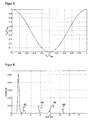
- FIG. 1 shows an exemplary, recorded by a TDR sensor 10 waveform from a level measurement in a container with two stacked media.
- the waveform is called an echo curve in the image caption, because it is the system's response to a transmit pulse.
- an ideal curve without parasitic effects, EMC interference or other noise sources is drawn.
- an at least reasonably smooth curve can be achieved by analog or digital filtering.
- the extrema of the signal curve are used to measure the distance to the interfaces and the relative permittivity or the relative dielectric constant of the media.
- a first maximum is a pure artifact and will not be discussed further.
- the following maximum 42 arises at the beginning of the probe 24, which is also referred to below as the line input, and serves as an initial reference pulse.
- the transmission signal is reflected at the first interface to the first medium or at the second interface to the second medium in the container 12. From the end of the probe 24 comes a last maximum 48 as the final reference pulse.
- the later signal components are no longer relevant, further smaller extrema are higher orders of multiple reflections at the two interfaces. It is conceivable to use these extremes for plausibility, but mostly they are not suitable because of too low signal / noise ratio.
- Each extremum 42-48 is described by two parameters as shown, namely the amplitude A start , A refl Wed. , A end and the temporal position t start , t refl Wed. , t end .
- the superscript running index Mi stands for the ith medium.
- the initial reference pulse 42, the final reference pulse 48 and the reflection pulse 44 closest to the initial reference pulse 42 are searched from the first interface. From their amplitudes and temporal positions, the relative dielectric constant of the first medium is determined in two ways. to then compare the results and decide whether there is another medium in the container 12 under the first medium.
- a first method determines the relative dielectric constant ⁇ r ⁇ 1 M ⁇ 1 from the amplitudes A start of the initial reference pulse 42 and A refl M ⁇ 1 of the reflection pulse 44 at the first interface.
- the index ri stands for relative dielectric constant according to the ith method.
- Z L is the wave impedance of the air-filled space above the first medium
- Z l is the wave impedance of the first medium.
- a second method determines the relative dielectric constant ⁇ r ⁇ 2 M ⁇ 1 again independent of the difference between the time t refl M ⁇ 1 of the first reflection pulse 44 and the time t end of the final reference pulse 48.
- ⁇ r ⁇ 1 M ⁇ 1 and ⁇ r ⁇ 2 M ⁇ 1 match up to a previously defined tolerance limit ⁇ M 1 , that is, if: ⁇ r ⁇ 2 M ⁇ 1 - ⁇ r ⁇ 1 M ⁇ 1 ⁇ ⁇ M ⁇ 1 ,
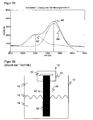
- FIG. 2 illustrates such a situation with two superimposed media 14a-b, which also the exemplary waveform of the FIG. 1 equivalent. It shows some of the parameters used.
- the first medium 14a is foam forming a first interface 18a
- the second media 14b forming a second interface 18b is a liquid.
- the top layer is formed by air.
- Z 1 denotes the wave impedance in the first medium 14a
- Z 2 denotes the wave impedance in the second medium 14b.
- the dielectric constant determined by the first method becomes ⁇ r ⁇ 1 M ⁇ 1 used because the determined according to the second method relative dielectric constant ⁇ r ⁇ 2 M ⁇ 1 under the has now been calculated as a false hypothesis that there is only one medium in the container 12.
- the relative dielectric constant ⁇ r M ⁇ 2 is a still unknown size.
- FIG. 2 also illustrates the relationship between the amplitudes A start and A refl M ⁇ 2 ,
- a pulse having the amplitude A start At the first interface 18a, a pulse having the amplitude A start .
- the pulse component which proceeds further towards the end of the probe depends solely on the reflection coefficient r M 1 of the first interface 18a and amounts to A start ⁇ ( r M 1 + 1).
- This pulse portion strikes the second interface 18b, and a portion of the pulse is reflected back towards the first interface 18a.
- Its amplitude additionally depends on the reflection coefficient r M 2 of the second interface 18b and is A start ⁇ ( r M 1 + 1).
- r M 2 The returning wave hits the first interface 18a a second time from the opposite direction. In turn, a portion is reflected, while the remaining portion runs back towards the line input.
- r M ⁇ 2 A refl M ⁇ 2 A begin ⁇ r M ⁇ 1 + 1 2 ,
- the results become ⁇ r ⁇ 1 M ⁇ 2 and ⁇ r ⁇ 2 M ⁇ 2 Both methods compared with a tolerance threshold ⁇ M 2 .
- the measurement is with the results d begin M ⁇ 1 .
- d begin M ⁇ 2 for the distances to the two interfaces 18a-b and the relative dielectric constant ⁇ r M ⁇ 1 .
- ⁇ r M ⁇ 2 for the two media 14a-b, the latter corresponding, for example, to the result of one of the two methods or an average of both methods.
- a further medium below the second medium 14b is assumed.
- the procedure is repeated iteratively until all existing media have been found or until an abort condition is met.
- the further iterations will only be briefly described in order to give generalized calculation instructions for the nth medium.
- d end Mn L - d begin Mn ,
- reflection pulses 44, 46 In order to estimate the parameters of reflection pulses 44, 46 as accurately as possible, it is provided in a development of the invention to operate the amplifier 38 with a non-linear characteristic. If the reflection pulses 44, 46 are then uniquely identified, the known effect of the non-linear amplification should be eliminated before quantitative evaluations of amplitude values.
- FIG. 4 represents the effect of amplification with a characteristic according to FIG. 3 on the waveform of the FIG. 1
- the two reflection pulses 44, 46 can obviously be separated better, because apart from the initial artifact no disturbing extrema occur more. However, already well-pronounced pulses like the initial artifact pulse are unnecessarily amplified disproportionately.
- the characteristic curve is therefore preferably to be adapted such that the amplitudes of the reflection pulses 44, 46 at the boundary surfaces are purposefully amplified and the remaining pulses are suppressed.
- a plurality of preferably continuously differentiable functions can be pieced together in order to specifically achieve the desired amplification of mean amplitudes in which measuring pulses 44, 46 lie and suppression of artifacts and noise.
- Pulse 42-48 are now very clearly identifiable.
- the final reference pulse 48 is somewhat less pronounced, but because of the known probe length it can be searched for in a quite narrow time range and thus nevertheless reliably detected. As long as the characteristic is monotonic, the position of the pulses 42-48 under non-linear amplification is maintained.
- Deviating and non-symmetrical non-linear characteristics can be defined according to the described guidelines.
- any piecewise function curves are conceivable, such as polynomial, exponential, logarithmic, hyperbolic or trigonometric functions.
- the discrete measured values are interpolated to obtain an analytical function and to increase the measuring accuracy of the sensor beyond the temporal resolution of the sampling times.
- a polynomial interpolation is not effective.
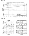
- FIG. 9 shows the waveform of the FIG. 1 mirrored and discretized on the Y axis and a sinc (x) interpolation for comparison.
- FIG. 10 is an enlarged detail, where the upper right of the entire waveform is shown in a pictogram with a rectangle 50, which indicates the position of the cutout. This form of representation is used in all subsequent detail enlargements to explain the interpolation. Of the FIG. 10 It can be seen that the sinc (x) interpolation generates relatively large interpolation errors despite its high cost.
- Another conceivable interpolation method consists in the piecewise interpolation using splines, in particular cubic C 2 -splines, which are thus twice continuously differentiable including their connection points.
- splines in particular cubic C 2 -splines, which are thus twice continuously differentiable including their connection points.
- FIGS. 11 and 12 demonstrate spline interpolation for the waveform in accordance with FIG. 1 very well. This quality is, however, bought by high numerical effort.
- a piecewise quadratic interpolation is used.
- FIGS. 11 and 12 In addition to spline interpolation, the just-derived piecewise quadratic interpolation is shown as a reference. In a section with greater variability according to FIG. 11 So larger gradients between each two nodes, the two interpolations are not distinguishable from each other. In the flatter section of the FIG. 12 On the other hand, in the piecewise quadratic interpolation, slight overshoots occur at the interpolation points introducing a small interpolation error. Note the different scale of the FIGS. 11 and 12 in Y-direction, the signal in FIG. 12 looks visually steeper than it is.
- a quadratic polynomial is used if the difference of the associated amplitude values exceeds a certain value ⁇ .
- the difference between the amplitude values of at least one of the two value pairs and the amplitude value at an additional support point in the environment must be a minimum value ⁇ . If these conditions are not met, the piece s i ( x ) is approximated by a linear polynomial.
- FIGS. 13 and 14 show again the excerpts of the FIGS. 11 and 12 with the difference that instead of the piecewise quadratic interpolation now the piecewise quadratic / linear interpolation is used.
- FIG. 13 Therefore, no differences are to be expected, because in this section the slope condition for quadratic interpolation is not violated or only in very few places, so that practically only quadratic interpolation comes into play.
- FIG. 14 a clear improvement recognizable.
- the linear approximation in areas of small slope does not show the disturbing overshoots and thus leads to a significantly lower interpolation error with even comparatively lower computational effort.
- the interpolation error is even greater than with spline interpolation. In the flat areas, however, the interpolation error is more acceptable anyway, since no reflection pulses 44, 46 are to be expected here.
- the different scale of FIGS. 13 and 14 in the Y direction Again, the different scale of FIGS. 13 and 14 in the Y direction.
- interpolation points ( x i , y i ) are taken into account if the difference between the amplitude maximum and minimum in an environment [ x i - ⁇ , x i + ⁇ ] of the interpolation point exceeds a minimum amount ⁇ : Max ⁇ y i - ⁇ ... y i + ⁇ - min ⁇ y i - ⁇ ... y i + ⁇ ⁇ ⁇ ⁇
- s j x ⁇ a j ⁇ x - x j 2 + b j ⁇ x - x j + c j .
- FIG. 15 shows the discretized waveform with the adaptive interpolation just described.
- ⁇ ⁇ x was set.
- no more support points are available. It should be noted that such subareas without support points can reach a considerable proportion of the total number of support points with a larger probe length.
- FIG. 16 shows a part of the FIG. 15 in a region with large slopes, which interpolates with quadratic polynomials.
- the relevant quantities, namely amplitude and position of the maximum, can be clearly seen.
- FIG. 17 provides a comparison of the FIG. 15 in a low slope area. Due to the opposite FIG. 16 changed scale in the Y direction, the remaining slope of the waveform is still visually exaggerated. Almost all interpolation points are ignored and are bridged by a linear interpolation.
- the described adaptive interpolation avoids unnecessary effort in irrelevant subareas. interesting parts, on the other hand, are interpolated very precisely. The effort compared to spline interpolation or even sinc interpolation is considerably reduced. All described interpolation methods are equally applicable to linearly as well as non-linearly pre-amplified signal waveforms.
- the measurement of the distance to several interfaces requires that the individual reflection pulses 44, 46 are resolved exactly and their amplitude and position are determined as accurately as possible. This is particularly difficult when a medium forms a particularly thin layer, so that the reflection pulses of two interfaces overlap one another. A simple search for extremes not only runs the risk of overlooking an interface. Because of the deviant waveform of superimposed reflection pulses, the position of the maximum and thus its amplitude may also be incorrectly evaluated.
- FIG. 18 shows three conceivable special cases in which two reflection pulses are superimposed.
- the waveforms are linear or not amplified, in the right part of the FIG. 18 on the other hand reinforced with a non-linear characteristic.
- the earlier reflection pulse is less pronounced and leads only to an upstream shoulder of the later reflection pulse.
- a second special case is the temporal reflection to this, where the later reflection pulse is less pronounced and leads to a downstream shoulder.
- the two reflection pulses are completely fused into a single maximum.
- FIG. 19 shows the three special cases of the left part of the FIG. 18 , ie the linearly amplified signal waveforms, after this interpolation.
- the left part of the FIG. 19 represents the complete waveforms and the right part of the FIG. 19 the cutouts 50 is enlarged.
- FIG. 20 is analogous to the FIG. 19 Here are the three special cases of the right part of the FIG. 18 are based, so the non-linearly amplified signal waveforms. Again, the left part of the FIG. 20 the complete waveforms and the right part of the FIG. 20 the cutouts 50 are enlarged. In the non-linear amplification, the local maxima to be found are more distinguishable.
- a minimum duration is searched for after the first rising edge and its last point as in FIG. 21 shown as the first reference maximum 54 set.
- the reference maximum begins as in FIG. 22 shown a time window that ends after a predetermined duration at a time 56.
- the time window is chosen to be so large that two reflection pulses merged into one another, but a separated next reflection pulse is no longer detected.
- the window width can be fixed in advance independently of the specific measurement because of the known individual pulse shape and an expected maximum amplitude.
- the time window is searched for a falling edge 58 over a minimum period.
- the exact position of the local maximum is then determined. Since the waveform is described by the interpolation function, the position can be determined analytically with high accuracy.
- FIG. 24 shows the thus separated reflection pulses, where in the left part of detail enlargements and in the right part of the complete signal waveforms in the three special cases are shown.
- the amplitudes belonging to the positions determined in this way can be read out directly from the interpolation function.
- the amplitudes can still be falsified by the superimposition.
- FIG. 25 An optimization method is explained with which the superposition of reflection pulses is separated into the individual reflection pulses. Shown is, on the one hand, the superimposed signal profile 60 and, on the other hand, the two individual reflection pulses 62, 64 which form the superimposition. In the example of FIG. 25 Accordingly, the number n of the superimposed reflection pulses is two. It can clearly be seen that the amplitudes, in particular the amplitude of the second reflection pulse 64, would be overestimated only on the basis of the superimposed signal profile 60 without the separation shown.
- the shape of the transmission pulse S (t) and thus a single reflection pulse is known or is measured in advance.
- the invention preferably seeks to search not quite generally for the entire probe length for a large number of media but, for example, only for a small time window for two media, as in the case of the figure 25.
- FIGS. 18 to 24 described very good initial values of the free parameters known. This or part of these measures cause an optimization algorithm to converge rapidly in the global maximum.
- both the distances to the interfaces and the relative dielectric constants of the respective media forming the interfaces are known.
- the number of media is basically unlimited.
- Simple level meters usually have only switching output signals. In the configuration of the simple interface, it could be determined depending on which medium level in boundary layer measurements or depending on the medium or foam level in applications with foam formation, the outputs are controlled. Thus, useful functions for the application of the sensor can be realized:
- a container in which a liquid forms foam still contains a foam layer when emptying.
- Simple level sensors interpret this foam layer as residual liquid. Since the sensor 10 according to the invention knows the relative dielectric constant, a distinction is made between a residual layer of the liquid and a pure foam layer. Thus, a dry running protection of pumps can be realized, and conventionally specially provided for this function additional sensors in the pump lines are dispensable.
- a similar case occurs at high levels with foam or multiple media. Overflow of a container can occur when a simple level sensor overlooks a foam surface and only recognizes the underlying liquid surface with its comparatively high reflectivity. In contrast, the sensor according to the invention also dissolves the foam layer even including its layer thickness and can generate a switching signal as an overfill warning.
- the implementation of an overfill protection is desired for some applications, an approval according to WHG (Water Resources Act) even requires overfill protection.
- the determined relative dielectric constants can be used for quality control of the process in the container.
- the relative dielectric constants are made available to the application, for example via an interface, or the sensor offers corresponding setting possibilities for a signal at a switching output if certain criteria for the relative dielectric constants are violated or complied with.
- the sensor according to the invention recognizes but at the constant relative dielectric constant that within the same medium, another non-plausible reflection pulse is formed at the deposit.
- the sensor can already generate a warning or fault message at this time, in order to avoid the error situation later, when the level drops below the deposit. Such self-monitoring protects the system against further damage and increases its availability.
Description
Die Erfindung betrifft ein Verfahren zur Messung der Entfernung zu mindestens einer ersten Grenzfläche und zur Bestimmung der relativen Dielektrizitätskonstante eines die erste Grenzfläche bildenden ersten Mediums nach dem Oberbegriff von Anspruch 1 sowie einen Sensor, der zur Ausführung des Verfahrens ausgebildet ist, nach dem Oberbegriff von Anspruch 15.The invention relates to a method for measuring the distance to at least a first interface and for determining the relative dielectric constant of the first interface forming the first medium according to the preamble of
Es ist aus vielen Anwendungen bekannt, den Abstand zu einer Grenzfläche aus der Laufzeit eines Mikrowellensignals zu bestimmen. Eine Möglichkeit ist, das Signal frei abzustrahlen, wie dies beim Radar geschieht. Wegen der unkontrollierten Wellenausbreitung wird häufig das Verfahren der Zeitbereichsreflektometrie (TDR, Time Domain Reflectometry) bevorzugt. Es basiert auf der Bestimmung von Laufzeiten eines elektromagnetischen Signals, um den Abstand einer Diskontinuität des Leitungswellenwiderstandes wie etwa eines Kabelbruchs oder einer Grenzfläche zwischen zwei Medien zu ermitteln. Der Unterschied zum Radar besteht darin, dass die elektromagnetischen Wellen nicht ins Freie abgestrahlt, sondern entlang eines Leiters geführt werden.It is known from many applications to determine the distance to an interface from the transit time of a microwave signal. One way is to radiate the signal freely, as happens with the radar. Because of the uncontrolled wave propagation, the Time Domain Reflectometry (TDR) method is often preferred. It is based on the determination of propagation times of an electromagnetic signal to determine the distance of a continuity of the line resistance, such as a cable break or an interface between two media. The difference to the radar is that the electromagnetic waves are not emitted to the outside, but are guided along a conductor.
Eine der ältesten Anwendungen des TDR-Prinzips ist die Lokalisierung von Brüchen in Überseeleitungen. Man kann TDR ebenso nutzen, um Füllstände in einem Behälter zu bestimmen, Leitungen in elektronischen Schaltungen zu testen oder um für Bauplanung oder Landwirtschaft den Feuchtigkeitsgehalt des Erdbodens in bestimmten Tiefen zu bestimmen. Für Anwendungen zur Füllstandsmessung ist der Leiter als Monosonde oder Koaxialsonde ausgebildet, welche senkrecht oder schräg in den Tank eingeführt wird und möglichst dicht bis zum Boden reicht, um den vollen Messbereich abzudecken.One of the oldest applications of the TDR principle is the localization of breaks in overseas pipelines. TDR can also be used to determine levels in a tank, to test pipelines in electronic circuits, or to determine the moisture content of the soil at specific depths for construction planning or agriculture. For level measurement applications, the conductor is designed as a monoprobe or coaxial probe, which is inserted vertically or obliquely into the tank and as close as possible to the bottom to cover the full range.
Bei einer TDR-Messung wird ein sehr kurzer elektrischer Sendeimpuls in den Leiter eingespeist und durchläuft ihn in Richtung des gegenüberliegenden Endes. Trifft der Impuls auf eine Störstelle, was gleichbedeutend mit einer Änderungen des örtlichen Wellenwiderstand ist, wird ein Teil der Sendeenergie zum Leitungseingang zurückreflektiert. Aus der Laufzeit zwischen dem Aussenden des Sendeimpulses und dem Empfang der Reflexion lässt sich die Position der Störstelle ortsgenau errechnen. Ein wichtiges Beispiel einer Störstelle ist eine Grenzfläche, welche zwei räumliche Bereiche mit unterschiedlichen physikalischen oder chemischen Eigenschaften trennt, wie eine Grenzfläche zwischen zwei Medien.In a TDR measurement, a very short electrical transmit pulse is fed into the conductor and passes through it towards the opposite end. The impulse hits an impurity, which is equivalent to a change of the local Characteristic impedance, part of the transmission energy is reflected back to the line input. From the transit time between the transmission of the transmitted pulse and the reception of the reflection, the position of the defect can be calculated in a location-specific manner. An important example of an impurity is an interface that separates two spatial regions with different physical or chemical properties, such as an interface between two media.
Um den Empfangszeitpunkt genau bestimmen zu können, wird der Verlauf des Empfangssignals abgetastet und einer digitalen Auswertung zugeführt. Dabei werden lokale Extremstellen im Signalverlauf gesucht und deren zeitliche Lage einer Reflexion an einer Grenzfläche zugeordnet.In order to be able to determine the time of reception precisely, the course of the received signal is sampled and fed to a digital evaluation. In this case, local extreme points are searched in the signal course and assigned their temporal position of a reflection at an interface.
Schwierigkeiten entstehen, wenn mehrere Grenzflächen vorhanden sind, wie dies beispielsweise bei mehreren Medien in einem Behälter der Fall ist. Dabei kann es sich beispielsweise um Wasser handeln, das sich am Boden eines Öltanks ansammelt, oder um Schaum, der sich an der Oberfläche einer Flüssigkeit bildet. Prinzipiell entstehen zwar an jeder Grenzfläche Reflexionen, und die jeweiligen Laufzeiten bis zu jeder dieser Grenzfläche lassen sich auch in eine Entfernung umrechnen. Dazu sind aber zwei Voraussetzungen zu erfüllen: Die relative Dielektrizitätskonstante der jeweiligen Medien muss bekannt sein, weil sie die Laufzeit und damit die Umrechnung in eine Entfernung beeinflusst, und es muss die zeitliche Lage der Reflexionssignale in dem Signalverlauf aufgelöst werden. Ersteres ist unflexibel, und darüber hinaus lässt sich beispielsweise im Falle von Schaum die relative Dielektrizitätskonstante gar nicht immer vorab angeben, da sie von der Zusammensetzung des Schaums abhängt. Letzteres ist besonders bei dünnen Schichtungen der Medien problematisch, weil sich dort die Reflexionssignale überlagern können. Außerdem nimmt die Energie der Reflexionssignale mit jeder Grenzfläche weiter ab, so dass sie sich weniger aus dem Rauschpegel erheben.Difficulties arise when multiple interfaces are present, as is the case with multiple media in a container, for example. This may be, for example, water that accumulates at the bottom of an oil tank, or foam that forms on the surface of a liquid. In principle, reflections arise at each interface, and the respective transit times up to each of these interfaces can also be converted into a distance. However, there are two prerequisites to be met: The relative dielectric constant of the respective media must be known because it influences the transit time and thus the conversion into a distance, and the temporal position of the reflection signals in the signal profile must be resolved. The former is inflexible, and moreover, for example, in the case of foam, the relative dielectric constant can not always be given in advance since it depends on the composition of the foam. The latter is particularly problematic in thin layers of the media, because there can superimpose the reflection signals. In addition, the energy of the reflection signals decreases further with each interface, so that they rise less from the noise level.
Ein herkömmlicher Auswertealgorithmus, der nur für die Erkennung einzelner Reflexionssignale ausgelegt ist, kann diese überlagerten Reflexionssignale nicht trennen. Da die Kurvenform von der erwarteten Kurvenform einzelner Reflexionssignale abweicht, kann sogar der Fall auftreten, dass ein überlagertes Reflexionssignal gar nicht detektiert wird. Jedenfalls wird ein solcher Algorithmus die zwei Grenzflächen nicht erkennen und wegen der abweichenden Kurvenform die zeitliche Lage ungenau bestimmen. Die Folge sind unvollständige Informationen über die Grenzflächen, ungenaue Messergebnisse oder sogar das Fehlen jeglicher Messwerte bei Nichterkennung einer Grenzfläche.A conventional evaluation algorithm, which is designed only for the detection of individual reflection signals, can not separate these superimposed reflection signals. Since the waveform differs from the expected waveform of individual reflection signals, it may even be the case that a superimposed reflection signal is not detected at all. In any case, such an algorithm will not recognize the two interfaces and, due to the deviant waveform, inaccurately determine the temporal position. The result is incomplete information about the interfaces, inaccurate readings, or even the absence of any non-boundary readings.
Aus der
Die
In der
In der
Schließlich ist ohne Zusammenhang mit Zeitbereichsreflektometrie beispielsweise aus der
Viele herkömmliche Verfahren sind somit gar nicht in der Lage, mit mehreren Grenzflächen umzugehen, da nur eine Extremstelle in dem Signalverlauf erwartet wird. Soweit der Stand der Technik überhaupt Aussagen über eine weitere Grenzfläche machen kann, sind zunächst kompliziertere Sondenformen notwendig, und dennoch lässt sich nur mit zusätzlichem Vorwissen die Entfernung der weiteren Grenzfläche bestimmen.Many conventional methods are thus not able to deal with multiple interfaces because only one extreme point in the waveform is expected. As far as the state of the art can make any statements about a further interface, more complicated probe forms are initially necessary, and yet can be determined only with additional prior knowledge, the removal of the other interface.
Es ist daher Aufgabe der Erfindung, ein verbessertes Verfahren zur Messung der Entfernung von Grenzflächen anzugeben, mit dem mehrere Grenzflächen auflösbar sind.It is therefore an object of the invention to provide an improved method for measuring the distance of interfaces, with the multiple interfaces are resolvable.
Diese Aufgabe wird durch ein Verfahren zur Messung der Entfernung zu mindestens einer ersten Grenzfläche sowie zur Bestimmung der relativen Dielektrizitätskonstante eines die erste Grenzfläche bildenden ersten Mediums nach Anspruch 1 sowie einen Sensor nach Anspruch 15 gelöst, der für die Ausführung des Verfahrens ausgebildet ist. Die Erfindung geht dabei von dem Grundgedanken aus, das jeweils oberste unbekannte Medium und dessen Grenzfläche auszumessen und die so gewonnene Information zu verwenden, um die weiteren Medien und Grenzflächen zu bestimmen. Dabei wird anders als herkömmlich nicht nur ein einziges besonders ausgeprägtes Reflexionssignal gesucht, sondern auch der übrige Signalverlauf ausgewertet.This object is achieved by a method for measuring the distance to at least a first interface as well as for determining the relative dielectric constant of a first interface forming the first medium according to
Nach der erfindungsgemäßen Lösung wird durch einen Vergleich zweier Messungen der relativen Dielektrizitätskonstante, nämlich einmal vom Sondenanfang bis zu der ersten Grenzfläche und einmal von der ersten Grenzfläche bis zum Sondenende, festgestellt, ob es noch weitere Medien und damit weitere Grenzflächen gibt. Die Laufzeit des Signals unterhalb der ersten Grenzschicht wird nämlich davon beeinflusst, ob sich dort nur das erste Medium oder noch weitere Medien mit anderer relativer Dielektrizitätskonstante befinden. Stimmen daher die beiden Messungen über eine Toleranz hinaus nicht überein, so wird auf die Anwesenheit eines weiteren Mediums geschlossen. Liefern umgekehrt beide Messungen innerhalb der Toleranzen denselben Wert der relativen Dielektrizitätskonstanten, so gibt es nur ein Medium der somit zuverlässig bestimmten Dielektrizitätskonstanten.According to the solution of the invention, a comparison of two measurements of the relative dielectric constant, namely once from the beginning of the probe to the first interface and once from the first interface to the end of the probe, determines whether there are any other media and thus further interfaces. The transit time of the signal below the first boundary layer is in fact influenced by whether there are only the first medium or other media with a different relative dielectric constant. If, therefore, the two measurements do not agree beyond a tolerance, then the presence of a further medium is concluded. Conversely, if both measurements within the tolerances supply the same value of the relative dielectric constant, then there is only one medium of the thus reliably determined dielectric constant.
Die Erfindung hat den Vorteil, dass keinerlei Vorwissen über die Grenzflächen und die Medien erforderlich ist. Das Verfahren ist in der Lage, eine prinzipiell beliebige Anzahl von unbekannten Medien in beliebiger Schichtung und Schichtdicke zuverlässig aufzulösen. Dabei wird außerdem noch eine höhere Messgenauigkeit erreicht. Da zugleich die relative Dielektrizitätskonstante der Medien bestimmt wird, kann das Verfahren zusätzlich eine Aussage über die Art der Medien treffen, sofern eine Tabelle hinterlegt wird, die den relativen Dielektrizitätskonstanten Materialien zuordnet.The invention has the advantage that no prior knowledge of the interfaces and the media is required. The method is capable of reliably resolving any number of unknown media in any desired layering and layer thickness. In addition, a higher measurement accuracy is achieved. Since at the same time the relative dielectric constant of the media is determined, the method can additionally make a statement about the type of media, provided that a table is deposited, which assigns materials to the relative dielectric constant.
Eine bevorzugte Anwendung ist die Messung von Füllständen in einem Behälter mit einem Medium oder mehreren übereinander geschichteten Medien. Dabei zeigt das Beispiel von Schaum, dass vorab nicht bekannt ist, ob und inwieweit eine zusätzliche Schicht eines weiteren Mediums und damit eine weitere Grenzfläche entsteht. Genaugenommen bildet nicht ein Medium allein eine Grenzfläche, sondern die Grenzfläche trennt das jeweilige Medium von einem darüber liegenden Medium, wobei die Grenzfläche zugleich die untere Fläche dieses darüber liegenden Mediums ist. Da die Zuordnung aber auch durch eines der Medien eindeutig ist, wenn man die Grenzfläche jeweils als die zu dem Sender nähere Grenzfläche definiert, wird das jeweilige darüber liegende Medium zur sprachlichen Vereinfachung meist nicht erwähnt.A preferred application is the measurement of levels in a container with one or more media stacked on top of one another. The example of foam shows that it is not known in advance whether and to what extent an additional layer of another medium and thus an additional interface is formed. Strictly speaking, not a medium alone forms an interface, but the interface separates the respective medium from an overlying medium, wherein the interface at the same time is the lower surface of this overlying medium. However, since the assignment is also unambiguous by one of the media, if one defines the interface in each case as the interface closer to the transmitter, the respective overlying medium is usually not mentioned for linguistic simplification.
Die bevorzugte Signalform sind kurze Sendepulse. Denkbar sind aber auch andere Signalformen, die eine gute zeitliche Auflösung zulassen, indem sie beispielsweise mindestens eine steile Flanke aufweisen. Üblicherweise werden Mikrowellensignale verwendet.The preferred waveform is short transmit pulses. However, other signal forms are also conceivable which allow a good temporal resolution, for example by having at least one steep edge. Usually, microwave signals are used.
Die relative Dielektrizitätskonstante wird bevorzugt bei dem ersten Mal unter Verwendung eines Reflexionskoeffizienten 


Die Entfernung ![]()
![]()
![]()
![]()
![]()
![]()


![]()
![]()

![]()
![]()
![]()
![]()
![]()
![]()
![]()
![]()
![]()
![]()
Die Entfernung ![]()
![]()
![]()
![]()
![]()
![]()
![]()


![]()
![]()

![]()
![]()
![]()
![]()
![]()
![]()
![]()
![]()
![]()
Vorteilhafterweise werden keine weiteren Grenzflächen gesucht, wenn mindestens eines der folgenden Abbruchkriterien erfüllt ist:
- es wurde eine Maximalanzahl von Grenzflächen gefunden,
- die größte erkannte und noch keiner Grenzfläche zugeordnete Amplitude in dem Signalverlauf unterschreitet eine Amplitudenschwelle,
- der Signalverlauf innerhalb eines vorgegebenen Zeitbereich ist vollständig ausgewertet,
- die von dem Beginn der Sonde bis zu der zuletzt ausgewerteten Grenzfläche aufintegrierte Energie des Signalverlaufs überschreitet eine Energieschwelle.
- a maximum number of interfaces was found
- the largest recognized amplitude, which has not yet been assigned to an interface, in the signal profile falls below an amplitude threshold,
- the waveform within a given time range is fully evaluated,
- the energy of the signal waveform integrated from the beginning of the probe to the last evaluated interface exceeds an energy threshold.
Der Signalverlauf wird auf hinreichend ausgeprägte Extremstellen untersucht, deren Anzahl unmittelbar mit der Anzahl von auflösbaren Grenzschichten korrespondiert. Da aber nach dem Passieren mehrerer Grenzschichten ein weiteres Reflexionssignal nicht mehr in allen Fällen eindeutig von einem Rauschausschlag unterscheidbar ist, werden hiermit weitere Kriterien angegeben, die einerseits von vorne herein die messbare Anzahl von Grenzflächen beschränken oder die abschätzen, ob überhaupt noch ein hinreichendes Signal/Rauschverhältnis für weitere auflösbare Grenzflächen gegeben ist.The signal profile is examined for sufficiently pronounced extreme positions, the number of which corresponds directly to the number of resolvable boundary layers. Since, however, after passing through several boundary layers, a further reflection signal is no longer clearly distinguishable from a noise excursion in all cases, hereby further criteria are specified which on the one hand restrict the measurable number of interfaces on the one hand or estimate whether there is still a sufficient signal / Noise ratio is given for other resolvable interfaces.
Der Signalverlauf des reflektierten Signals wird bevorzugt mit einer nichtlinearen Kennlinie verstärkt aufgezeichnet, bei der Eingangssignale mittlerer Amplitude überproportional verstärkt werden, wobei mittlere Amplituden dadurch definiert sind, dass sie in einem Intervall oberhalb eines Rauschpegels und unterhalb eines Startsignals oder eines Artefakts vom Ende der Sonde als den stärksten zu erwartenden Signale liegen. Somit sind die auszuwertenden Reflexionssignale in dem Signalverlauf von Anfang an stärker ausgeprägt, und die Auswertung wird erheblich erleichtert.The waveform of the reflected signal is preferably amplified with a non-linear characteristic in which mid-amplitude input signals are amplified disproportionately, with mean amplitudes being defined by an interval above a noise level and below a start signal or artefact from the end of the probe the strongest signals to be expected. Thus, the reflection signals to be evaluated in the waveform are more pronounced from the beginning, and the evaluation is greatly facilitated.
Der Signalverlauf des reflektierten Signals wird bevorzugt mit einer nichtlinearen Kennlinie verstärkt aufgezeichnet, bei der Eingangssignale kleiner Amplitude und/oder großer Amplitude unterdrückt werden, wobei kleine Amplituden als unterhalb oder in der Nähe eines Rauschpegels und große Amplituden als in der Größenordnung eines Startsignals oder eines Artefakts vom Ende der Sonde definiert sind. Die nichtlineare Kennlinie unterdrückt Anteile des Signalverlaufs, die ohnehin keinem zu messenden Reflexionssignal entsprechen können. Auch dadurch wird das Auffinden der Reflexionssignale vereinfacht.The waveform of the reflected signal is preferably amplified with a non-linear characteristic in which small amplitude and / or large amplitude input signals are suppressed, with small amplitudes as below or near a noise level and large amplitudes on the order of a start signal or artifact are defined by the end of the probe. The non-linear characteristic suppresses portions of the signal profile which can not correspond to a reflection signal to be measured anyway. This also simplifies finding the reflection signals.
Die Kennlinie ist bevorzugt für minimale und maximale Eingangssignale flach bei einem Bruchteil maximaler Verstärkung, liegt für Eingangssignale um Null bei Null und hat dazwischen einen sigmoiden Verlauf, wobei der sigmoide Verlauf insbesondere durch ein Polynom vorgeschrieben ist und wobei die Anschlussstellen des Polynoms zu den flachen Bereichen zumindest stetig differenzierbar sind. Ein solches Polynom ist leicht parametrierbar und implementiert die in den vorangehenden Absätzen beschriebene nichtlineare Kennlinie, welche dem Reflexionssignal entsprechende Eingangssignale mittlerer Amplituden verstärkt und Störsignale niedriger oder hoher Amplituden unterdrückt. Die Kennlinie kann symmetrisch zur Mittelachse mit dem Eingangssignal Null sein, oder es werden unterschiedliche Polynome und Anschlussstellen der Polynome für positive und negative Eingangssignale definiert, um beispielsweise positive Signale wie einen Referenzpuls am Anfang des Signalverlaufs oder einen Artefaktpuls am Ende des Signalverlaufs anders zu behandeln als negative Signale, wie sie bei Reflexionen an einer Grenzfläche entstehen.The characteristic is preferred for minimum and maximum input signals shallow at a fraction of maximum gain, zero around zero for input signals, and has a sigmoidal course therebetween, the sigmoidal characteristic being dictated by a polynomial in particular, and the polynomial's junctions to the flat regions are at least continuously differentiable. Such a polynomial is easily parameterizable and implements the non-linear characteristic described in the preceding paragraphs, which amplifies mid-amplitude input signals corresponding to the reflection signal and suppresses low or high amplitude spurious signals. The characteristic curve can be symmetrical to the central axis with the input signal Zero or different polynomials and junctions of the polynomials are defined for positive and negative input signals, for example, to treat positive signals such as a reference pulse at the beginning of the waveform or an artifact pulse at the end of the waveform differently than negative signals, as in reflections on a Interface arise.
Der Signalverlauf wird bevorzugt zunächst mit diskreten Stützstellen digitalisiert und anschließend stückweise durch eine Schar von Polynomen zweiter Ordnung zwischen je zwei Stützstellen interpoliert, wobei die Anschlussstellen zwischen zwei Polynomen stetig differenzierbar sind. Diese Polynome sollten nicht mit dem Polynom der Verstärkerkennlinie verwechselt werden, sie haben nichts miteinander zu tun. Durch die Interpolation wird der diskrete Signalverlauf analytisch zugänglich, und zugleich sind Messwerte mit höherer Auflösung als der Abtastrate des A/D-Wandlers möglich. Das Interpolationsverfahren gemäß dieser und den im Folgenden noch vorgestellten Ausführungsformen eignet sich besonders auch in dem Fall, in dem die Abtastzeitpunkte nicht äquidistant sind. Bekannte Interpolationsverfahren wie eine sinc(x)-Interpolation können mit derartigen nicht äquidistanten Messdaten nicht umgehen.The signal profile is preferably first digitized with discrete interpolation points and then interpolated piecewise by a family of polynomials of second order between every two interpolation points, wherein the interpolation points between two polynomials are continuously differentiable. These polynomials should not be confused with the polynomial of the amplifier characteristic, they have nothing to do with each other. The interpolation makes the discrete signal path analytically accessible, and at the same time, measurements with higher resolution than the sampling rate of the A / D converter are possible. The interpolation method according to this and the embodiments presented below is particularly suitable also in the case where the sampling times are not equidistant. Known interpolation methods such as sinc (x) interpolation can not handle such non-equidistant measurement data.
Bevorzugt wird zwischen je zwei Stützstellen, in denen die Steigung des Signalverlaufs unterhalb einer ersten Mindeststeigung liegt, anstelle eines Polynoms zweiter Ordnung ein Polynom erster Ordnung für die Interpolation verwendet. Bereiche geringer Steigung weisen mit hoher Wahrscheinlichkeit keine Reflexionssignale auf und sind daher für die Auswertung nicht interessant. Eine Interpolation mit Geradenstücken an diesen Stellen sorgt überdies für einen insgesamt glatteren Kurvenverlauf.Preferably, a polynomial of first order is used for interpolation instead of a second-order polynomial between every two support points in which the slope of the signal path is below a first minimum slope. Areas of low slope are very likely to have no reflection signals and are therefore not interesting for the evaluation. An interpolation with straight sections at these points also ensures an overall smoother curve.
Vorteilhafterweise bleibt dann, wenn in der Umgebung einer Stützstelle die Steigung des Signalverlaufs unterhalb einer zweiten Mindeststeigung liegt, die Stützstelle in der weiteren Interpolation unberücksichtigt. Mit einer solchen adaptiven Interpolation wird der Rechenaufwand und der erforderliche Speicherplatz verringert, indem in für die Messwerte in aller Regel unwichtigen Bereichen anstelle zweier oder mehrerer sehr flache Geradenstücke oder Parabelbögen ein Geradenstück mittlerer Steigung verwendet wird. Die erste Mindeststeigung sollte bevorzugt größer sein als die zweite Mindeststeigung, da ansonsten keine Geradenstücke vorkommen könnten, sondern entsprechende Bereiche unmittelbar unberücksichtigt blieben.Advantageously, when in the vicinity of a support point, the slope of the signal waveform is below a second minimum slope, the support point in the further interpolation is disregarded. Such adaptive interpolation reduces the computational effort and space required by using a mid-slope straight line instead of two or more very flat straight line segments or parabola arcs in regions that are generally unimportant for the measured values. The first minimum slope should preferably be greater than the second minimum slope, since otherwise no straight line pieces could occur, but corresponding areas were immediately disregarded.
Die Signallaufzeiten ![]()
![]()
Bevorzugt werden die Maxima in einem Durchlauf des Signalsverlaufs von links nach rechts und in einem Durchlauf des Signalverlaufs von rechts nach links ermittelt. Damit werden ineinander verschmolzene Reflexionssignale sowohl in dem Falle gefunden, dass ein kleines Reflexionssignal einem größeren Reflexionssignal vorhergeht, wie dass es ihm nachfolgt. Die auf Positionen bezogenen Begrifflichkeiten orientieren sich an einer grafischen Darstellung des Signalverlaufs. Eigentlich müsste man von zeitlichen Richtungen, also früheren und späteren Ereignissen sprechen, aber Position und Zeit sind bei bekannten relativen Dielektrizitätskonstanten unmittelbar ineinander umrechenbar.Preferably, the maxima are determined in a passage of the signal curve from left to right and in a passage of the signal curve from right to left. Thus, reflection signals fused together are found both in the case that a small reflection signal precedes a larger reflection signal as follows. The terms related to positions are based on a graphical representation of the signal curve. Actually one would have to speak of temporal directions, ie earlier and later events, but position and time are directly interconvertible with known relative dielectric constants.
Die genaue Lage der Maxima wird bevorzugt analytisch aus einer Interpolation des Signalverlaufs ermittelt. Das ist ein weiterer großer Vorteil der Interpolation, denn damit sind Auflösungen weit unterhalb der Abtastrate des diskreten Signalverlaufs mit sehr einfachen analytischen Extremwertbestimmungen möglich.The exact position of the maxima is preferably determined analytically from an interpolation of the signal profile. This is another great advantage of interpolation, as it enables resolutions far below the sampling rate of the discrete waveform with very simple analytical extremum determinations.
In bevorzugter Weiterbildung wird ein Soll-Signalverlauf aus einer Faltung des Sendesignals mit durch die Amplituden ![]()
![]()
![]()
![]()
![]()
![]()
![]()
![]()
![]()
![]()
![]()
![]()
![]()
![]()
![]()
![]()
Die Erfindung wird nachstehend auch hinsichtlich weiterer Vorteile und Merkmale unter Bezugnahme auf die beigefügte Zeichnung anhand von Ausführungsbeispielen erläutert. Die Figuren der Zeichnung zeigen in:
- Fig. 1
- ein beispielhafter von einem TDR-Sensor aufgezeichneter Signalverlauf mit Erläuterung der Parameter Amplitude und zeitliche Lage der Reflexionssig- nale;
- Fig. 2
- eine schematische Darstellung einer beispielhaften Schichtung zweier Me- dien mit Erläuterung weiterer Parameter und der Berechnung der Amplitu- de der Reflexionssignale;
- Fig. 3
- eine beispielhafte nichtlineare Kennlinie zur Signalverstärkung in Form ei- ner Parabel;
- Fig. 4
- ein beispielhafter Signalverlauf bei Verstärkung mit der Kennlinie gemäß
Figur 3 ; - Fig. 5
- eine beispielhafte nichtlineare Kennlinie zur Signalverstärkung in Form ei- nes Cosinus;
- Fig. 6
- ein beispielhafter Signalverlauf bei Verstärkung mit der Kennlinie gemäß
Figur 5 ; - Fig. 7
- eine beispielhafte nichtlineare Kennlinie zur Signalverstärkung in Form ei- ner zusammengesetzten Funktion aus flachen Bereichen und Polynomen;
- Fig. 8
- ein beispielhafter Signalverlauf bei Verstärkung mit der Kennlinie gemäß
Figur 7 ; - Fig. 9
- ein beispielhafter diskreter Signalverlauf und dessen Interpolation mittels eines Kardinalsinus;
- Fig. 10
- eine Ausschnittsvergrößerung aus dem Signalverlauf und der
Interpolation der Figur 9 ; - Fig. 11
- eine Ausschnittsvergrößerung eines beispielhaften diskreten Signalverlaufs und dessen Interpolation mittels Spline-Funktionen;
- Fig. 12
- eine Ausschnittsvergrößerung eines beispielhaften diskreten Signalverlaufs und dessen Interpolation mittels stückweise quadratischer Funktionen und Spline-Funktionen;
- Fig. 13
- eine Ausschnittsvergrößerung eines beispielhaften diskreten Signalverlaufs und dessen Interpolation mittels stückweise quadratisch/linearer Funktio- nen und Spline-Funktionen;
- Fig. 14
- eine Darstellung gemäß
Figur 13 in einem anderen Ausschnitt des Signal- verlaufs; - Fig. 15
- ein beispielhafter diskreter Signalverlauf bei adaptiver Interpolation mit un- berücksichtigten Stützstellen in Bereichen geringer Steigung;
- Fig. 16
- eine Ausschnittsvergrößerung aus dem Signalverlauf und der
Interpolation der Figur 15 ; - Fig. 17
- eine andere Ausschnittsvergrößerung aus dem Signalverlauf und der Inter- polation der
Figur 15 ; - Fig. 18
- im linken Teil die Darstellung dreier möglicher Sonderfälle ineinander ver- schmelzender Reflexionssignale, im rechten Teil die drei Sonderfälle bei nichtlinearer Verstärkung;
- Fig. 19
- im linken Teil die drei Sonderfälle des linken Teils der
Figur 18 bei adapti- ver Interpolation, im rechten Teil Ausschnittsvergrößerungen dazu; - Fig. 20
- im linken Teil die drei Sonderfälle des rechten Teils der
Figur 18 bei adapti- ver Interpolation, im rechten Teil Ausschnittsvergrößerungen hierzu; - Fig. 21
- Ausschnittsvergrößerungen ineinander verschmolzener Reflexionssignale in den drei Sonderfällen gemäß
Figur 18 zur Erläuterung der Lage eines ersten Maximums; - Fig. 22
- die Ausschnittsvergrößerungen der
Figur 21 mit Erläuterung des Auffindens fallender Flanken bei Auswertung von links nach rechts; - Fig. 23
- die Ausschnittsvergrößerungen der
Figur 21 mit Erläuterung des Auffindens fallender Flanken bei umgekehrter Auswertung von rechts nach links; - Fig. 24
- im linken Teil die Ausschnittsvergrößerung der
Figur 21 mit den gekenn- zeichneten Lagen sämtlicher Maxima der verschmolzenen Reflexionssig- nale, im rechten Teil entsprechende vollständige Signalverläufe; - Fig. 25
- eine Ausschnittsvergrößerung eines beispielhaften Signalverlaufs in einem ersten Sonderfall zur Erläuterung eines Optimierungsverfahrens zum Auf- finden von Amplitude und zeitlicher Lage der Reflexionssignale.
- Fig. 26
- eine schematische Darstellung eines TDR-Sensors in einer Anwendung als Füllstandssensor nach dem Stand der Technik;
- Fig. 27
- ein Blockschaltbild eines Sensorkopfes mit der Ansteuerung des
Sensors gemäß Figur 26 nach dem Stand der Technik;
- Fig. 1
- an example of a TDR sensor recorded waveform with explanation of the parameters amplitude and timing of the Reflexionssig- signals;
- Fig. 2
- a schematic representation of an exemplary layering of two media with explanation of other parameters and the calculation of the amplitude of the reflection signals;
- Fig. 3
- an exemplary non-linear characteristic for signal amplification in the form of a parabola;
- Fig. 4
- an exemplary waveform in amplification with the characteristic according to
FIG. 3 ; - Fig. 5
- an exemplary non-linear characteristic for signal amplification in the form of a cosine;
- Fig. 6
- an exemplary waveform in amplification with the characteristic according to
FIG. 5 ; - Fig. 7
- an exemplary non-linear characteristic for signal amplification in the form of a composite function of flat regions and polynomials;
- Fig. 8
- an exemplary waveform in amplification with the characteristic according to
FIG. 7 ; - Fig. 9
- an exemplary discrete waveform and its interpolation by means of a cardinal sine;
- Fig. 10
- an enlarged detail of the waveform and the interpolation of
FIG. 9 ; - Fig. 11
- an enlarged detail of an exemplary discrete waveform and its interpolation using spline functions;
- Fig. 12
- an enlarged detail of an exemplary discrete waveform and its interpolation using piecewise quadratic functions and spline functions;
- Fig. 13
- an enlarged detail of an exemplary discrete signal waveform and its interpolation by means of piecewise quadratic / linear functions and spline functions;
- Fig. 14
- a representation according to
FIG. 13 in another section of the signal path; - Fig. 15
- an exemplary discrete waveform in adaptive interpolation with disregarded nodes in areas of low slope;
- Fig. 16
- an enlarged detail of the waveform and the interpolation of
FIG. 15 ; - Fig. 17
- another section magnification from the waveform and the interpolation of
FIG. 15 ; - Fig. 18
- in the left part the representation of three possible special cases of merging reflection signals, in the right part the three special cases with non-linear amplification;
- Fig. 19
- in the left part the three special cases of the left part of the
FIG. 18 in the case of adaptive interpolation, in the right-hand part, enlargements to this; - Fig. 20
- in the left part the three special cases of the right part of the
FIG. 18 in the case of adaptive interpolation, in the right part enlargements on this; - Fig. 21
- Enlarged sections of fused reflection signals in the three special cases according to
FIG. 18 for explaining the position of a first maximum; - Fig. 22
- the detail enlargements of the
FIG. 21 with explanation of finding falling edges in evaluation from left to right; - Fig. 23
- the detail enlargements of the
FIG. 21 with explanation of finding falling edges in reverse evaluation from right to left; - Fig. 24
- in the left part the enlargement of the section
FIG. 21 with the marked positions of all maxima of the fused reflection signals, in the right part corresponding complete signal courses; - Fig. 25
- an enlarged detail of an exemplary waveform in a first special case to explain an optimization method for finding the amplitude and timing of the reflection signals.
- Fig. 26
- a schematic representation of a TDR sensor in an application as a level sensor according to the prior art;
- Fig. 27
- a block diagram of a sensor head with the control of the sensor according to
FIG. 26 According to the state of the art;
Der Sensor 10 weist einen Sensorkopf 20 mit einer Steuerung 22 auf, die vorzugsweise auf einer gemeinsamen Platine untergebracht ist. Alternativ sind mehrere über Stecker verbundene Leiterplatten oder Flexprintträger denkbar. An die Steuerung 22 ist eine koaxiale Sonde 24 angeschlossen, welche einen Außenleiter 26 und einen Innenleiter 28 aufweist. Bei einer solchen geschlossenen Sonde 24 werden die elektromagnetischen Signale besonders störungsfrei geführt. Es ist aber auch denkbar, eine andere Sondenform einzusetzen, beispielsweise eine offene Monosonde, die leichter gereinigt werden kann.The
Die in dem Sensorkopf 20 vorgesehene Steuerung 22 beziehungsweise ihre Platine ist in
Wie auch schon einleitend beschrieben, wird bei einer Messung ein Puls über einen Mikrowellensender 34 auf den Innenleiter 28 gegeben und die Laufzeit des an der Grenzfläche 18 entstehenden und in einem Mikrowellenempfänger 36 empfangenen Reflexpulses gemessen, um den Abstand der Grenzfläche 18 und damit den Füllstand in dem Behälter 12 zu ermitteln. Das Empfangssignal des Mikrowellenempfängers 36 wird für die Auswertung nach Verstärkung in einem Verstärker 38 mit einem Digital/Analogwandler 40 digitalisiert.As already described in the introduction, during a measurement, a pulse is transmitted to the
Erfindungsgemäß ist vorgesehen, die Entfernung zu mehr als einer Grenzfläche zu bestimmen. Die hierfür erforderlichen Auswertungsverfahren sind in der Auswertungseinheit 32 implementiert und werden im Folgenden anhand der
Für die Auswertung werden die Extrema des Signalverlaufs herangezogen, um die Entfernung zu den Grenzflächen und die relative Permittivität beziehungsweise die relative Dielektrizitätskonstante der Medien zu messen. Ein erstes Maximum ist ein reines Artefakt und wird nicht weiter diskutiert. Das folgende Maximum 42 entsteht am Anfang der Sonde 24, der im Folgenden auch als Leitungseingang bezeichnet wird, und dient als Anfangsreferenzimpuls. Bei den nachfolgenden beiden Minima 44, 46 wird das Sendesignal an der ersten Grenzfläche zu dem ersten Medium beziehungsweise an der zweiten Grenzfläche zu dem zweiten Medium in dem Behälter 12 reflektiert. Vom Ende der Sonde 24 stammt ein letztes Maximum 48 als Endreferenzimpuls. Die späteren Signalanteile sind nicht mehr relevant, weitere kleinere Extrema sind höhere Ordnungen von Mehrfachreflexionen an den beiden Grenzflächen. Es ist denkbar, diese Extrema zur Plausibilisierung heranzuziehen, aber zumeist sind sie dafür wegen zu geringem Signal/Rauschverhältnis nicht geeignet.For the evaluation, the extrema of the signal curve are used to measure the distance to the interfaces and the relative permittivity or the relative dielectric constant of the media. A first maximum is a pure artifact and will not be discussed further. The following
Jedes Extremum 42-48 wird wie dargestellt durch zwei Parameter beschrieben, nämlich die Amplitude Astart , ![]()
![]()
![]()
![]()
Zunächst werden nun der Anfangsreferenzimpuls 42, der Endreferenzimpuls 48 und der am nächsten bei dem Anfangsreferenzimpuls 42 gelegene Reflexionsimpuls 44 von der ersten Grenzfläche gesucht. Aus deren Amplituden und zeitlichen Lagen wird auf zweierlei Arten die relative Dielektrizitätskonstante des ersten Mediums bestimmt, um anschließend die Ergebnisse zu vergleichen und zu entscheiden, ob unter dem ersten Medium ein weiteres Medium in dem Behälter 12 vorhanden ist.First, the
Ein erstes Verfahren bestimmt die relative Dielektrizitätskonstante ![]()
![]()
![]()
![]()
Der Reflexionskoeffizient der ersten Grenzfläche r M1 beträgt 
![]()


![]()
Ein zweites Verfahren bestimmt die relative Dielektrizitätskonstante ![]()
![]()
![]()
![]()
![]()
![]()
![]()
![]()
Für die Entfernung ![]()
![]()

![]()
![]()
Unter Kenntnis der Sondenlänge L berechnet sich die Entfernung ![]()
![]()
![]()
![]()
Die Ausbreitungsgeschwindigkeit der elektromagnetischen Wellen in dem ersten Medium beträgt 
![]()

![]()
Unter der hypothetischen Voraussetzung, dass sich nur ein einziges Medium in dem Behälter 12 unterhalb der ersten Grenzfläche befindet, ergibt sich dann 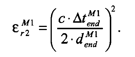
Um nun zu entscheiden, ob tatsächlich nur ein einziges Medium vorhanden ist oder ob ein weiteres Medium unter das erste Medium geschichtet ist, wird überprüft, ob ![]()
![]()
![]()
![]()
![]()
![]()
Es wird wegen möglicher Rundungsfehler, Quantisierungsfehler, Fehler in der Zeitbasis, also Schwankungen der Abtastzeitpunkte, Messfehler, Störeinflüsse auf das Messsignal oder andere parasitäre Effekte nur Gleichheit innerhalb der Toleranzgrenze ζ M1 gefordert. Ist die Gleichheit innerhalb der Toleranz ζ M1 gegeben, so befindet sich nur ein einziges Medium in dem Behälter 12. Seine relative Dielektrizitätskonstante ![]()
![]()
![]()
![]()
![]()
![]()
![]()
![]()
Ergibt sich andererseits ein Unterschied ![]()
![]()
![]()
![]()
![]()
![]()
![]()
![]()
![]()
![]()
![]()
![]()
Erneut werden die zwei unterschiedlichen Verfahren eingesetzt, um die Entfernung ![]()
![]()
![]()
![]()
Für das erste Verfahren wird der Reflexionskoeffizient rM2 an der zweiten Grenzfläche 18b in Kenntnis der relativen Dielektrizitätskonstanten ![]()

![]()
![]()
![]()
![]()
![]()
![]()
![]()
![]()
![]()
![]()
![]()
Die Amplituden Astart und ![]()

![]()
Folglich gilt aus der eingangs angegebenen Gleichung für r M2 
Für das zweite Verfahren zur Bestimmung der relativen Dielektrizitätskonstanten ![]()
![]()
![]()
![]()
![]()
![]()
Die Entfernung zwischen der ersten Grenzfläche 18a und zweiten Grenzfläche 18b beträgt folglich 
![]()
![]()
![]()
![]()
Erneut wird zunächst hypothetisch angenommen, dass unterhalb des zweiten Mediums 14b kein weiteres Medium und damit keine weitere Grenzschicht befindet. Dann gilt 

Wie schon an der ersten Grenzschicht 18a werden die Ergebnisse ![]()
![]()
![]()
![]()
![]()
![]()
![]()
![]()
![]()
![]()
![]()
![]()
Für weitere Medien wird das Vorgehen iterativ wiederholt, bis alle vorhandenen Medien gefunden wurden oder bis eine Abbruchbedingung erfüllt ist. Die weiteren Iterationen werden nur noch kurz beschrieben, um verallgemeinerte Rechenvorschriften für das n-te Medium anzugeben.For other media, the procedure is repeated iteratively until all existing media have been found or until an abort condition is met. The further iterations will only be briefly described in order to give generalized calculation instructions for the nth medium.
Der verallgemeinerte Reflexionskoeffizient rMn der n-ten Grenzfläche beträgt in Kenntnis der Reflexionskoeffizienten aller darüber liegende Grenzflächen 
Unter Verwendung von: 

Für das zweite Verfahren wird die Zeitdifferenz ![]()
![]()
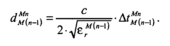
![]()

![]()
![]()
![]()
Die relative Dielektrizitätskonstante des n-ten Mediums berechnet sich zu 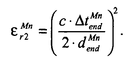
Wie oben für die erste und zweite Grenzfläche erläutert, wird anschließend geprüft, ob die Bedingung 
Neben dem genannten Abbruchkriterium, dass die mit jeweils zwei Verfahren bestimmten Dielektrizitätskonstanten innerhalb der geforderten Toleranzen übereinstimmen, sind auch andere Abbruchkriterien denkbar, wie beispielsweise eine Beschränkung der Anzahl an Medien, die gesucht werden soll, eine minimale erforderliche Amplitude des Reflexionspulses, da Störeinflüsse auf das Messsignal bei kleinen Amplituden zu einem hohen relativen Fehler führen, eine Begrenzung der zeitlichen Position der Reflexionspulse oder die Forderung, dass das bestimmte Integral über die Energie ![]()
![]()

![]()
![]()
Um die Parameter von Reflexionspulsen 44, 46 möglichst genau zu schätzen, ist in einer Weiterbildung der Erfindung vorgesehen, den Verstärker 38 mit einer nichtlinearen Kennlinie zu betreiben. Sind die Reflexionspulse 44, 46 dann eindeutig identifiziert, so sollte vor quantitativen Auswertungen von Amplitudenwerten der bekannte Effekt der nichtlinearen Verstärkung wieder herausgerechnet werden.In order to estimate the parameters of
Die Kennlinie ist deshalb bevorzugt so anzupassen, dass gezielt die Amplituden der Reflexionspulse 44, 46 an den Grenzflächen verstärkt und die übrigen Pulse unterdrückt werden. 
Dazu werden können beispielsweise mehrere bevorzugt stetig differenzierbare Funktionen stückweise zusammengesetzt werden, um gezielt die gewünschte Verstärkung mittlerer Amplituden, in denen Messpulse 44, 46 liegen, und Unterdrückung von Artefakten und Rauschen zu erreichen. Eine mögliche Kennlinie wird durch 
Die Wirkung der Kennlinie gemäß
Es können nach den beschriebenen Leitlinien abweichende, auch nicht-symmetrische nichtlineare Kennlinien definiert werden. Dabei sind prinzipiell beliebige stückweise Funktionsverläufe denkbar, wie polynomiale, exponentielle, logarithmische, hyperbolische oder trigonometrische Funktionen.Deviating and non-symmetrical non-linear characteristics can be defined according to the described guidelines. In principle, any piecewise function curves are conceivable, such as polynomial, exponential, logarithmic, hyperbolic or trigonometric functions.
Für die Signalverarbeitung steht nicht der gesamte analoge Signalverlauf, sondern nur eine endliche Anzahl diskreter Messwerte zu meist äquidistanten, durch die Abtastrate des A/D-Wandlers 40 gegebenen äquidistanten Zeitpunkten zur Verfügung. Für TDR-Sonden wird häufig noch eine als Zeitdehnung bekannte Unterabtastung vorgenommen, um die sehr kurzen Signalverläufe mit langsamerer Elektronik zu erfassen. Auf diese dem Fachmann geläufigen Verfahren soll hier aber nicht näher eingegangen werden.For the signal processing is not the entire analog waveform, but only a finite number of discrete measured values to most equidistant, given by the sampling rate of the A /
Die diskreten Messwerte werden interpoliert, um eine analytische Funktion zu gewinnen und die Messgenauigkeit des Sensors über die zeitliche Auflösung der Abtastzeitpunkte hinaus zu steigern. Eine polynomiale Interpolation ist dabei nicht zielführend. Zunächst müsste wegen der hohen Anzahl von Stützstellen ein Polynom sehr hoher Ordnung verwendet werden. Selbst wenn man den Aufwand hierfür in Kauf nimmt, bildet das Polynom die Zwischenwerte der Stützstellen aufgrund von Runges Phänomen sehr schlecht ab, so dass ein solches Interpolationspolynom für die Bestimmung von Reflexionspulsen 44, 46 weitgehend nutzlos ist. Selbst wenn man die Interpolation auf kleinere Bereiche des Signalverlaufs und einfache Polynome beispielsweise zweiter oder dritter Ordnung beschränkt, ergeben sich signifikante Abweichungen zwischen Signalverlauf und Interpolationspolynom.The discrete measured values are interpolated to obtain an analytical function and to increase the measuring accuracy of the sensor beyond the temporal resolution of the sampling times. A polynomial interpolation is not effective. First, because of the high number of nodes, a polynomial of very high order would have to be used. Even if one takes the effort for this into account, the polynomial maps the intermediate values of the interpolation points very poorly due to Runge's phenomenon, so that such an interpolation polynomial is largely useless for the determination of
Ein anderes denkbares Verfahren ist die sinc(x)-Interpolation. Das grundsätzliche Problem hierbei ist die Fensterung im Zeitbereich. Als Ausweg sind endliche Filter (FIR, Filter mit endlicher Impulsantwort) oder das Auffüllen mit Nullen (Zero padding) bekannt.Another conceivable method is the sinc (x) interpolation. The fundamental problem here is windowing in the time domain. As a way out finite filters (FIR, finite impulse response filters) or zero padding are known.
Ein anderes denkbares Interpolationsverfahren besteht in der stückweisen Interpolation unter Verwendung von Splines, insbesondere kubischen C 2-Splines, die also einschließlich ihrer Anschlussstellen zweimal stetig differenzierbar sind. Wie die Ausschnittsvergrößerungen der
In einer Ausführungsform der Erfindung wird deshalb eine stückweise quadratische Interpolation verwendet. Ein Kurvenstück zwischen zwei benachbarten Stützstellen wird dabei mit quadratischen Polynomen interpoliert: ![]()
![]()
Dabei bezeichnet si (x) das i-te Kurvenstück zwischen dem i-ten und (i+1) -ten Abtastpunkt, xi die diskreten Zeitpunkte und yi die diskreten Amplituden. Alle Polynome müssen drei Anforderungen erfüllen:
- 1. Die Interpolationsfunktion soll alle Messpunkte beinhalten → si (xi ) = yi
- 2. Die Interpolationsfunktion soll stetig sein → si (x i+1) = s i+1 (x i+1)
- 3. Die Interpolationsfunktion soll differenzierbar sein → si '(x i+1) = s i+1'(x i+1)
- 1. The interpolation function should contain all measuring points → s i ( x i ) = y i
- 2. The interpolation function should be continuous → s i ( x i +1 ) = s i +1 ( x i +1 )
- 3. The interpolation function should be differentiable → s i '( x i +1 ) = s i +1 ' ( x i +1 )
Aus diesen Bedingungen lässt sich ein Gleichungssystem ableiten:. ![]()
![]()
![]()
![]()
![]()
![]()
![]()
![]()
![]()
![]()
Dabei sind ai , bi und ci die Polynomkoeffizienten, δ i die Steigung zwischen zwei benachbarten Abtastpunkten und Δx deren zeitlicher Abstand. Diese Gleichungen werden nach ihren Koeffizienten aufgelöst: 
![]()
![]()

![]()
![]()
Für die Bestimmung des ersten Stücks der Interpolationsfunktion wird die Vereinfachung getroffen, dass dieses eine lineare Steigung hat, da es sonst unterbestimmt wäre, und es gilt zusätzlich c 1 = y 1, b 1 = δ1, α1 = 0.For the determination of the first part of the interpolation function, the simplification is made that it has a linear slope, otherwise it would be underdetermined, and additionally c 1 = y 1 , b 1 = δ 1 , α 1 = 0.
In die
Deshalb ist in einer Weiterbildung der Erfindung vorgesehen, die stückweise quadratische Interpolation durch eine Kombination aus quadratischer Interpolation in steilen und linearer Interpolation in flachen Teilbereichen zu ersetzen.Therefore, it is provided in a further development of the invention to replace the piecewise quadratic interpolation by a combination of quadratic interpolation in steep and linear interpolation in flat subregions.
Dabei wird folgende Rechenvorschrift verwendet: 
Für das Stück si (x) des Signalverlaufs zwischen den Wertepaaren (xi ,yi ) und (x i+1,y i+1) wird ein quadratisches Polynom verwendet, falls die Differenz der zugehörigen Amplitudenwerte einen bestimmten Wert ξ überschreitet. Zusätzlich kann gefordert werden, dass der Unterschied zwischen den Amplitudenwerten von mindestens einem der beiden Wertepaare und dem Amplitudenwert an einer zusätzlichen Stützstelle in der Umgebung einen Mindestwert ζ betragen muss. Falls diese Bedingungen nicht erfüllt sind, wird das Stück si (x) durch ein lineares Polynom approximiert.For the piece s i ( x ) of the signal course between the pairs of values ( x i , y i ) and ( x i +1 , y i +1 ), a quadratic polynomial is used if the difference of the associated amplitude values exceeds a certain value ξ. In addition, it may be required that the difference between the amplitude values of at least one of the two value pairs and the amplitude value at an additional support point in the environment must be a minimum value ζ. If these conditions are not met, the piece s i ( x ) is approximated by a linear polynomial.
Das Stück des Signalverlaufs wird weiterhin durch ![]()
![]()
![]()
![]()
![]()
![]()
Die Koeffizienten bi und a i werden aber in beiden Fällen unterschiedlich berechnet, nämlich für linear interpolierte Stücke des Signalverlaufs bi = δ i , ai = 0 und für quadratisch interpolierte Kurvenstücke bi = 2·δ i - b i-1, 
Die
Wie ein Blick auf ![]()
![]()
Die verbleibenden Stützstellen werden im Folgenden einem anderen Laufindex zugeordnet. Diese werden als (xj ,yj ) bezeichnet, und ihre Anzahl M ist kleiner oder gleich der originalen Anzahl an Stützstellen N: ![]()
![]()
Die in den bisherigen Ausführungsformen konstante Differenz Δx der Lage der Stützstellen in x-Richtung wird dann durch hj = x j+1 -xj ersetzt und für die Wahl linearer oder quadratischer Interpolation zwischen den verbleibenden Stützstellen die folgende Fallunterscheidung in Abhängigkeit von einer vorgebbaren Mindeststeigung ν getroffen. 
Mit den Koeffizienten aj, bj und cj der allgemeinen Interpolationsfunktion ![]()
![]()

![]()

![]()
![]()
![]()
Bei dieser Abbildung ist deutlich zu sehen, dass bei dem Reflexionspuls eine quadratische Interpolation durchgeführt wurde. Dabei sind zeitliche Position und Amplitude des Maximums bei der Reflexionsstelle deutlich zu erkennen.In this figure, it can be clearly seen that quadratic interpolation was performed on the reflection pulse. The time position and amplitude of the maximum at the reflection point can be clearly seen.
Die beschriebene adaptive Interpolation vermeidet unnötigen Aufwand in irrelevanten Teilbereichen. Interessante Teilbereiche dagegen werden sehr genau interpoliert. Dabei ist der Aufwand gegenüber Spline-Interpolation oder gar sinc-Interpolation erheblich reduziert. Alle beschriebenen Interpolationsmethoden sind gleichermaßen auf linear wie nichtlinear vorverstärkte Signalverläufe anwendbar.The described adaptive interpolation avoids unnecessary effort in irrelevant subareas. Interesting parts, on the other hand, are interpolated very precisely. The effort compared to spline interpolation or even sinc interpolation is considerably reduced. All described interpolation methods are equally applicable to linearly as well as non-linearly pre-amplified signal waveforms.
Die Messung der Entfernung zu mehreren Grenzflächen setzt voraus, dass die einzelnen Reflexionspulse 44, 46 genau aufgelöst und deren Amplitude und Lage möglichst genau bestimmt werden. Dies bereitet besonders dann Schwierigkeiten, wenn ein Medium eine besonders dünne Schicht bildet, so dass die Reflexionspulse zweier Grenzflächen einander überlagern. Eine einfache Suche nach Extrema läuft dann nicht nur Gefahr, eine Grenzfläche zu übersehen. Wegen der abweichenden Kurvenform überlagerter Reflexionspulse wird dabei möglicherweise auch die Lage des Maximums und damit auch dessen Amplitude falsch bewertet.The measurement of the distance to several interfaces requires that the
Das erfindungsgemäße Verfahren zum Auffinden der Reflexionspulse verwendet bevorzugt die oben beschriebene adaptive linear/quadratische Interpolation.
Das Verfahren zum Auffinden der Reflexionspulse wird nun unter Bezugnahme auf die
Mit dem Referenzmaximum beginnt wie in
In dem Zeitfenster wird nach einer fallenden Flanke 58 über eine Mindestdauer gesucht. Zwischen Referenzmaximum 54 und Beginn der fallenden Flanke 58 wird anschließend die genaue Lage des lokalen Maximums bestimmt. Da der Signalverlauf durch die Interpolationsfunktion beschrieben wird, ist die Lage analytisch mit hoher Genauigkeit bestimmbar.In the time window is searched for a falling
Um nun die weiteren überlagerten Referenzpulse aufzufinden, wird das Krümmungsverhalten zwischen dem Referenzmaximum 54 und dem Ende der fallenden Flanke 58 untersucht. Ist eine Krümmungsänderung vorhanden, wie beispielsweise im ersten Sonderfall, so wird das bisher beschriebene Verfahren mit der Suche eines neuen Maximums, beginnend mit dem bereits gefundenen Maximum, wiederholt. Dies illustriert das oberster Drittel der
Gibt es keine Krümmungsänderung, so könnte sich wie im Sonderfall 2 ein weiterer Reflexionspuls mit einer niedrigeren Amplitude hinter dem gefundenen Maximum befinden. Das Verfahren wird dann wie in den beiden unteren Dritteln der
Die Amplituden können aber noch durch die Überlagerung verfälscht sein. Anhand der
Die Form des Sendepulses S(t) und damit eines einzelnen Reflexionspulses ist bekannt oder wird vorab ausgemessen. Die beiden zu bestimmenden Parameter des i-ten Reflexionspulses sind dessen Amplitude ![]()
![]()


![]()
![]()
Selbstverständlich sind andere Maße für die Güte der Übereinstimmung verwendbar. Algorithmen, welche die optimale Wahl der Parameter ![]()
![]()
![]()
![]()
Ein häufiges Problem derartiger Optimierungen ist, dass sie nicht oder nur lokal konvergieren. Deshalb sieht die Erfindung bevorzugt vor, nicht ganz allgemein über die gesamte Sondenlänge nach einer großen Anzahl von Medien zu suchen, sondern beispielsweise nur über ein kleines Zeitfenster nach zwei Medien, wie in dem Fall der Figur 25. Außerdem sind über die oben im Zusammenhang mit
Erfindungsgemäß sind somit sowohl die Entfernungen zu den Grenzflächen als auch die relativen Dielektrizitätskonstanten der jeweiligen die Grenzflächen bildenden Medien bekannt. Dabei ist die Anzahl der Medien prinzipiell unbeschränkt. Diese deutlich erweiterten Messwerte eröffnen für Anwendungen als Füllstandssensor neue Funktionen.Thus, according to the invention, both the distances to the interfaces and the relative dielectric constants of the respective media forming the interfaces are known. The number of media is basically unlimited. These significantly enhanced readings provide new functionality for level sensor applications.
Einfache Füllstandmesser haben in der Regel nur Schaltausgangssignale. Bei der Konfiguration des einfachen Interface könnte festgelegt werden, in Abhängigkeit welcher Mediumspegel bei Grenzschichtmessungen oder in Abhängigkeit des Mediums-oder Schaumpegels bei Applikationen mit Schaumbildung die Ausgänge angesteuert werden. Damit sind nutzbringende Funktionen für die Anwendung des Sensors realisierbar:Simple level meters usually have only switching output signals. In the configuration of the simple interface, it could be determined depending on which medium level in boundary layer measurements or depending on the medium or foam level in applications with foam formation, the outputs are controlled. Thus, useful functions for the application of the sensor can be realized:
Ein Behälter, in dem eine Flüssigkeit Schaum bildet, enthält beim Leerlaufen immer noch eine Schaumschicht. Einfache Füllstandssensoren interpretieren diese Schaumschicht als Restflüssigkeit. Da der erfindungsgemäße Sensor 10 die relative Dielektrizitätskonstante kennt, wird zwischen einer Restschicht der Flüssigkeit und einer reinen Schaumschicht unterschieden. Damit lässt sich ein Trockenlaufschutz von Pumpen realisieren, und herkömmlich eigens für diese Funktion vorgesehene zusätzliche Sensoren in den Pumpenleitungen werden verzichtbar.A container in which a liquid forms foam still contains a foam layer when emptying. Simple level sensors interpret this foam layer as residual liquid. Since the
Ein ähnlicher Fall tritt bei hohen Füllständen mit Schaum beziehungsweise mehreren Medien auf. Es kann zu einem Überlaufen eines Behälters kommen, wenn ein einfacher Füllstandssensor eine Schaumoberfläche übersieht und nur die darunter liegende Flüssigkeitsoberfläche mit ihrer vergleichsweise hohen Reflektivität erkennt. Der erfindungsgemäße Sensor dagegen löst auch die Schaumschicht sogar einschließlich ihrer Schichtdicke auf und kann ein Schaltsignal als Überfüllwarnung generieren. Die Realisierung einer Überfüllsicherung ist für einige Anwendungen gewünscht, eine Zulassung nach WHG (Wasserhaushaltsgesetz) fordert sogar eine Überfüllsicherung.A similar case occurs at high levels with foam or multiple media. Overflow of a container can occur when a simple level sensor overlooks a foam surface and only recognizes the underlying liquid surface with its comparatively high reflectivity. In contrast, the sensor according to the invention also dissolves the foam layer even including its layer thickness and can generate a switching signal as an overfill warning. The implementation of an overfill protection is desired for some applications, an approval according to WHG (Water Resources Act) even requires overfill protection.
Eine Kombination aus Überfüllwarnung aufgrund einer Schaumoberfläche und Trockenlaufschutz ist denkbar, insbesondere bei Geräten, die mehrere Schaltausgangssignale bereitstellen. Ebenso ist die analoge oder digitale Ausgabe von Füllständen aller oder einiger Medien möglich.A combination of overfill warning due to a foam surface and dry run protection is conceivable, especially for devices that provide multiple switching output signals. Similarly, the analog or digital output of levels of all or some media is possible.
Die ermittelten relativen Dielektrizitätskonstanten können für eine Qualitätskontrolle des Prozesses in dem Behälter genutzt werden. Dazu werden die relativen Dielektrizitätskonstanten beispielsweise über eine Schnittstelle für die Anwendung zugänglich gemacht, oder der Sensor bietet entsprechende Einstellmöglichkeiten für ein Signal an einem Schaltausgang, wenn gewisse Kriterien für die relativen Dielektrizitätskonstanten verletzt oder eingehalten werden.The determined relative dielectric constants can be used for quality control of the process in the container. For this purpose, the relative dielectric constants are made available to the application, for example via an interface, or the sensor offers corresponding setting possibilities for a signal at a switching output if certain criteria for the relative dielectric constants are violated or complied with.
Weiterhin ist möglich, anhand des Auftretens zusätzlicher oder fehlender Trennschichten einen Fehler in dem Prozess oder den Medien zu erkennen. Beispielsweise sind einige Flüssigkeiten hygroskopisch, und in Behältern lagert sich deshalb unten Wasser ab. Hier ist das Vorhandensein einer nicht erwarteten Trennschicht nutzbar, um eine Überwachung auf Ablagerungen zu realisieren.Furthermore, it is possible to detect an error in the process or the media based on the occurrence of additional or missing separation layers. For example, some liquids are hygroscopic, and so water is deposited in containers below. Here, the presence of an unexpected separation layer can be used to realize a deposit monitoring.
Schließlich ist auch eine Eigenüberwachung auf Verschmutzungen der Sonde möglich, insbesondere bei Verwendung einer geschlossenen Sonde wie einer Koaxialsonde. Besonders bei Anwendung zur Regelung von Pegelständen ist oftmals nur ein sehr enger Toleranzbereich vorgesehen. Deshalb setzen sich Schwebstoffe und Verunreinigungen in einem kleinen Bereich der Sonde in der Nähe des Pegelstands ab. Diese Verunreinigungen können stark genug sein, um ein Reflexionssignal zu erzeugen, welches als Grenzschichtreflexion interpretiert wird. Das bleibt zunächst unproblematisch, solange sich die Mediumsoberfläche im Bereich der Ablagerung befindet. Sinkt jedoch die Mediumsoberfläche ab, könnte ein einfacher Sensor das Niveau der Ablagerung fehlerhaft als Füllstand melden.Finally, a self-monitoring for contamination of the probe is possible, especially when using a closed probe such as a coaxial probe. Especially when used to control water levels is often provided only a very narrow tolerance range. Therefore, particulates and contaminants settle in a small area of the probe near the water level. These contaminants can be strong enough to produce a reflection signal, which is interpreted as boundary layer reflection. This remains unproblematic as long as the medium surface is in the area of the deposit. However, if the media surface decreases, a simple sensor could erroneously report the level of the deposit as a level.
Mit dem erfindungsgemäßen Vorgehen wird aber erkannt, dass sich nach der ersten Reflexion weiterhin ein Medium mit einer relativen Dielektrizitätskonstante von etwa Eins befindet, also offensichtlich Luft. Das ist unplausibel und kann zur Generierung einer Störungsmeldung verwendet werden.With the procedure according to the invention, however, it is recognized that, after the first reflection, there continues to be a medium with a relative dielectric constant of approximately one, that is to say obviously air. This is implausible and can be used to generate a fault message.
Bei ansteigendem Medium ist die Situation zwar weniger kritisch, da erstes Reflexionssignal und erste Grenzfläche übereinstimmen. Der erfindungsgemäße Sensor erkennt aber an der gleichbleibenden relativen Dielektrizitätskonstante, dass innerhalb desselben Mediums ein weiterer nicht plausibler Reflexionspuls an der Ablagerung entsteht. Der Sensor kann bereits zu diesem Zeitpunkt eine Warn- oder Störungsmeldung generieren, um später die Fehlersituation zu vermeiden, wenn der Füllstand unter die Ablagerung sinkt. Mit derartigen Eigenüberwachungen wird die Anlage vor weiteren Schäden bewahrt und deren Verfügbarkeit erhöht.With increasing medium, the situation is less critical, since the first reflection signal and the first interface coincide. The sensor according to the invention recognizes but at the constant relative dielectric constant that within the same medium, another non-plausible reflection pulse is formed at the deposit. The sensor can already generate a warning or fault message at this time, in order to avoid the error situation later, when the level drops below the deposit. Such self-monitoring protects the system against further damage and increases its availability.
Claims (15)
- A method for measuring the distance to at least a first boundary surface (18a) by transmitting an electromagnetic signal along a probe (24), recording the signal course of the reflected signal and determining the distance (


characterized in that
the relative dielectric constant (


- The method according to claim 1,
wherein the relative dielectric constant is determined at the first time with use of a reflection coefficient


- The method according to claim 1 or 2,
wherein the distance (


(

- The method according to any of the preceding claims,
wherein the distance (


- The method according to any of the preceding claims,
wherein no further boundary surfaces are located when at least one of the following termination criteria is met:- a maximum number of boundary surfaces (18a-b) was located;- the largest detected amplitude in the signal course not yet associated with a boundary surface (18a-b) is below an amplitude threshold,- the signal course within a preset time interval is completely evaluated,- the energy of the signal course integrated from the beginning of the probe (24) up to the last evaluated boundary surface exceeds an energy threshold. - The method according to any of the preceding claims,
wherein the signal course of the reflected signal is recorded with an amplification with a nonlinear characteristic curve that disproportionately amplifies input signals of medium amplitude, wherein medium amplitudes are defined in that they are in an interval above a noise level and below a start signal (42) or an artifact (48) from the probe end (24) that are the strongest expected signals. - The method according to any of the preceding claims,
wherein the signal course of the reflected signal is recorded with an amplification with a nonlinear characteristic curve that suppresses input signals of small amplitude and/or large amplitude, wherein small amplitudes are defined as below or near a noise level and large amplitudes are defined as being of an order of magnitude with a start signal (42) or an artifact (48) from the probe end (24). - The method according to claim 6 or 7,
wherein the characteristic curve is flat at a fraction of the maximum gain for minimal and maximal input signals, is zero for input signals near zero, and has a sigmoidal shape in between, wherein the sigmoidal shape is in particular prescribed by a polynom, wherein the connections of the polynom to the flat regions are at least continuously differentiable. - The method according to any of the preceding claims,
wherein the signal course is at first digitized with discrete sampling points and subsequently piecewise interpolated by a set of second order polynoms between two respective sampling points, wherein the connections between two polynoms are continuously differentiable. - The method according to any of the preceding claims,
wherein between each two sampling points in which the slope of the signal course is below a first minimum slope a first order polynom is used instead of a second order polynom for the interpolation. - The method according to any of the preceding claims,
wherein, when in a vicinity of a sampling point the slope of the signal curve is below a second minimum slope, the sampling point is disregarded in the further interpolation. - The method according to any of the preceding claims,
wherein the signal times of flight (
- The method according to any of the preceding claims,
wherein the precise position of the maxima is determined analytically from an interpolation of the signal course. - The method according to any of the preceding claims,
wherein a desired signal course is formed from a convolution of the transmission signal with delta pulses weighted with the amplitudes (


- A sensor (10), in particular a TDR level sensor, comprising a transmitter (34) and a receiver (36) for the transmission and reception of an electromagnetic signal, in particular a micro wave signal, and with a control (32) that is configured to determine the distance (


characterized in that
the control (32) is configured to determine the distance (

Priority Applications (1)
| Application Number | Priority Date | Filing Date | Title |
|---|---|---|---|
| EP20100154636 EP2365302B1 (en) | 2010-02-25 | 2010-02-25 | Measurement of the distance to at least one initial boundary area |
Applications Claiming Priority (1)
| Application Number | Priority Date | Filing Date | Title |
|---|---|---|---|
| EP20100154636 EP2365302B1 (en) | 2010-02-25 | 2010-02-25 | Measurement of the distance to at least one initial boundary area |
Publications (2)
| Publication Number | Publication Date |
|---|---|
| EP2365302A1 EP2365302A1 (en) | 2011-09-14 |
| EP2365302B1 true EP2365302B1 (en) | 2012-05-23 |
Family
ID=42320089
Family Applications (1)
| Application Number | Title | Priority Date | Filing Date |
|---|---|---|---|
| EP20100154636 Active EP2365302B1 (en) | 2010-02-25 | 2010-02-25 | Measurement of the distance to at least one initial boundary area |
Country Status (1)
| Country | Link |
|---|---|
| EP (1) | EP2365302B1 (en) |
Families Citing this family (11)
| Publication number | Priority date | Publication date | Assignee | Title |
|---|---|---|---|---|
| US8746045B2 (en) * | 2006-11-17 | 2014-06-10 | Meggitt (Orange County), Inc. | System and method for identifying fluids and monitoring fluid quality in a vessel |
| DE102012101725A1 (en) | 2012-03-01 | 2013-09-05 | Sick Ag | Method for level measurement |
| US8963769B2 (en) | 2012-10-16 | 2015-02-24 | Magnetrol International, Incorporated | Guided wave radar interface measurement medium identification |
| DK2759813T3 (en) | 2013-01-25 | 2016-06-06 | Sick Ag | Method and sensor for measuring the fill level of layered media |
| DE102013107847A1 (en) * | 2013-07-23 | 2015-01-29 | Endress + Hauser Gmbh + Co. Kg | Method for determining and monitoring the level of a medium in a container according to a transit time measurement method |
| DE102014103212A1 (en) * | 2014-03-11 | 2015-09-17 | Sick Ag | Sensor and method for detecting an object located on a roller conveyor |
| DE102015118917A1 (en) * | 2015-11-04 | 2017-05-04 | Finetek Co., Ltd. | Material level measuring method with a material level measuring device |
| JP7073344B2 (en) * | 2016-08-22 | 2022-05-23 | ビーエーエスエフ ソシエタス・ヨーロピア | Methods and equipment for identifying deposits in the mechanism's piping system |
| US10386180B2 (en) * | 2016-11-28 | 2019-08-20 | Honeywell International Inc. | Apparatus and method for measuring thin material thicknesses in inventory management applications |
| DE102017108702A1 (en) | 2017-04-24 | 2018-10-25 | Krohne S. A. S. | Method for determining the level and level gauge |
| US10816384B2 (en) * | 2017-10-31 | 2020-10-27 | Rosemount Tank Radar Ab | Radar level gauge system and method for interface measurement |
Family Cites Families (3)
| Publication number | Priority date | Publication date | Assignee | Title |
|---|---|---|---|---|
| GB2153616B (en) * | 1984-02-01 | 1987-03-11 | Standard Telephones Cables Ltd | Liquid level measurement |
| US5884231A (en) * | 1995-12-21 | 1999-03-16 | Endress & Hauser Gmbh & Co. | Processor apparatus and method for a process measurement signal |
| US6198424B1 (en) * | 1999-01-21 | 2001-03-06 | Rosemount Inc. | Multiple process product interface detection for a low power radar level transmitter |
-
2010
- 2010-02-25 EP EP20100154636 patent/EP2365302B1/en active Active
Also Published As
| Publication number | Publication date |
|---|---|
| EP2365302A1 (en) | 2011-09-14 |
Similar Documents
| Publication | Publication Date | Title |
|---|---|---|
| EP2365302B1 (en) | Measurement of the distance to at least one initial boundary area | |
| EP2634541B1 (en) | Method for measuring fill levels | |
| EP2652462B1 (en) | Measuring device, control device and measuring instrument for level measurement | |
| EP2759813B1 (en) | Method and sensor for measuring the fill level of layered media | |
| EP2366983B1 (en) | Mobility recognition in filling level measurement devices | |
| WO2015018586A1 (en) | Dispersion correction for fmcw radar in a pipe | |
| EP2652465B1 (en) | Determination of media characteristics during filling level measurement | |
| EP2527805B1 (en) | Evaluation device and method for determining a parameter for the position of a boundary area in a container | |
| DE112006002310T5 (en) | Processing of the tank signal in a radar level measurement system | |
| EP2179273B1 (en) | Method and device for humidity and/or density measurement | |
| EP2626676B1 (en) | Apparatus and method for correcting an offset | |
| EP2554956B1 (en) | Tracking taking mobility into consideration | |
| WO2008080840A1 (en) | Method for determining and monitoring the filling level of a medium in a container according to a propagation time measurement method | |
| EP1412710A1 (en) | Method for evaluating the measuring signals of a propagation-time based measuring device | |
| WO2007122116A1 (en) | Method for determining and monitoring the level of a medium in a container | |
| DE102007060579A1 (en) | Method for determining and / or assessing the filling state of a container filled with at least one medium | |
| DE102009001010A1 (en) | Method for determining and monitoring the level of a medium in a container according to a transit time measurement method | |
| EP3025128B1 (en) | Method for determining and monitoring the level of a medium in a container according to a transit time measurement method | |
| DE102010042525A1 (en) | Method for determining and monitoring the level of a medium in a container by means of a level gauge according to a transit time measurement method | |
| EP2527804A1 (en) | Method for recognising multiple and ground echoes | |
| EP2327966B1 (en) | Measurement of the distance of a boundary surface | |
| EP2584324B1 (en) | Fill level measuring device and method for determining a functional correlation between different tracks | |
| EP2182380B1 (en) | Method for detecting peak overlays in a discrete spectrum of a location signal | |
| DE10211334B4 (en) | A method of measuring effective directivity and / or effective source turret fitting of a system calibrated vectorial network analyzer and calibration standard set | |
| EP2739945B1 (en) | Fill level measuring device and method for determining a functional correlation between different tracks |
Legal Events
| Date | Code | Title | Description |
|---|---|---|---|
| PUAI | Public reference made under article 153(3) epc to a published international application that has entered the european phase |
Free format text: ORIGINAL CODE: 0009012 |
|
| AK | Designated contracting states |
Kind code of ref document: A1 Designated state(s): AT BE BG CH CY CZ DE DK EE ES FI FR GB GR HR HU IE IS IT LI LT LU LV MC MK MT NL NO PL PT RO SE SI SK SM TR |
|
| AX | Request for extension of the european patent |
Extension state: AL BA RS |
|
| 17P | Request for examination filed |
Effective date: 20111012 |
|
| GRAP | Despatch of communication of intention to grant a patent |
Free format text: ORIGINAL CODE: EPIDOSNIGR1 |
|
| GRAS | Grant fee paid |
Free format text: ORIGINAL CODE: EPIDOSNIGR3 |
|
| GRAA | (expected) grant |
Free format text: ORIGINAL CODE: 0009210 |
|
| AK | Designated contracting states |
Kind code of ref document: B1 Designated state(s): AT BE BG CH CY CZ DE DK EE ES FI FR GB GR HR HU IE IS IT LI LT LU LV MC MK MT NL NO PL PT RO SE SI SK SM TR |
|
| REG | Reference to a national code |
Ref country code: GB Ref legal event code: FG4D Free format text: NOT ENGLISH |
|
| REG | Reference to a national code |
Ref country code: CH Ref legal event code: EP |
|
| REG | Reference to a national code |
Ref country code: AT Ref legal event code: REF Ref document number: 559284 Country of ref document: AT Kind code of ref document: T Effective date: 20120615 |
|
| REG | Reference to a national code |
Ref country code: IE Ref legal event code: FG4D Free format text: LANGUAGE OF EP DOCUMENT: GERMAN |
|
| REG | Reference to a national code |
Ref country code: SE Ref legal event code: TRGR |
|
| REG | Reference to a national code |
Ref country code: DE Ref legal event code: R096 Ref document number: 502010000779 Country of ref document: DE Effective date: 20120719 |
|
| REG | Reference to a national code |
Ref country code: NL Ref legal event code: VDEP Effective date: 20120523 |
|
| REG | Reference to a national code |
Ref country code: LT Ref legal event code: MG4D Effective date: 20120523 |
|
| PG25 | Lapsed in a contracting state [announced via postgrant information from national office to epo] |
Ref country code: IS Free format text: LAPSE BECAUSE OF FAILURE TO SUBMIT A TRANSLATION OF THE DESCRIPTION OR TO PAY THE FEE WITHIN THE PRESCRIBED TIME-LIMIT Effective date: 20120923 Ref country code: CY Free format text: LAPSE BECAUSE OF FAILURE TO SUBMIT A TRANSLATION OF THE DESCRIPTION OR TO PAY THE FEE WITHIN THE PRESCRIBED TIME-LIMIT Effective date: 20120523 Ref country code: NO Free format text: LAPSE BECAUSE OF FAILURE TO SUBMIT A TRANSLATION OF THE DESCRIPTION OR TO PAY THE FEE WITHIN THE PRESCRIBED TIME-LIMIT Effective date: 20120823 Ref country code: FI Free format text: LAPSE BECAUSE OF FAILURE TO SUBMIT A TRANSLATION OF THE DESCRIPTION OR TO PAY THE FEE WITHIN THE PRESCRIBED TIME-LIMIT Effective date: 20120523 Ref country code: LT Free format text: LAPSE BECAUSE OF FAILURE TO SUBMIT A TRANSLATION OF THE DESCRIPTION OR TO PAY THE FEE WITHIN THE PRESCRIBED TIME-LIMIT Effective date: 20120523 |
|
| PG25 | Lapsed in a contracting state [announced via postgrant information from national office to epo] |
Ref country code: SI Free format text: LAPSE BECAUSE OF FAILURE TO SUBMIT A TRANSLATION OF THE DESCRIPTION OR TO PAY THE FEE WITHIN THE PRESCRIBED TIME-LIMIT Effective date: 20120523 Ref country code: PT Free format text: LAPSE BECAUSE OF FAILURE TO SUBMIT A TRANSLATION OF THE DESCRIPTION OR TO PAY THE FEE WITHIN THE PRESCRIBED TIME-LIMIT Effective date: 20120924 Ref country code: LV Free format text: LAPSE BECAUSE OF FAILURE TO SUBMIT A TRANSLATION OF THE DESCRIPTION OR TO PAY THE FEE WITHIN THE PRESCRIBED TIME-LIMIT Effective date: 20120523 Ref country code: GR Free format text: LAPSE BECAUSE OF FAILURE TO SUBMIT A TRANSLATION OF THE DESCRIPTION OR TO PAY THE FEE WITHIN THE PRESCRIBED TIME-LIMIT Effective date: 20120824 Ref country code: HR Free format text: LAPSE BECAUSE OF FAILURE TO SUBMIT A TRANSLATION OF THE DESCRIPTION OR TO PAY THE FEE WITHIN THE PRESCRIBED TIME-LIMIT Effective date: 20120523 |
|
| PG25 | Lapsed in a contracting state [announced via postgrant information from national office to epo] |
Ref country code: SK Free format text: LAPSE BECAUSE OF FAILURE TO SUBMIT A TRANSLATION OF THE DESCRIPTION OR TO PAY THE FEE WITHIN THE PRESCRIBED TIME-LIMIT Effective date: 20120523 Ref country code: NL Free format text: LAPSE BECAUSE OF FAILURE TO SUBMIT A TRANSLATION OF THE DESCRIPTION OR TO PAY THE FEE WITHIN THE PRESCRIBED TIME-LIMIT Effective date: 20120523 Ref country code: DK Free format text: LAPSE BECAUSE OF FAILURE TO SUBMIT A TRANSLATION OF THE DESCRIPTION OR TO PAY THE FEE WITHIN THE PRESCRIBED TIME-LIMIT Effective date: 20120523 Ref country code: EE Free format text: LAPSE BECAUSE OF FAILURE TO SUBMIT A TRANSLATION OF THE DESCRIPTION OR TO PAY THE FEE WITHIN THE PRESCRIBED TIME-LIMIT Effective date: 20120523 Ref country code: CZ Free format text: LAPSE BECAUSE OF FAILURE TO SUBMIT A TRANSLATION OF THE DESCRIPTION OR TO PAY THE FEE WITHIN THE PRESCRIBED TIME-LIMIT Effective date: 20120523 Ref country code: RO Free format text: LAPSE BECAUSE OF FAILURE TO SUBMIT A TRANSLATION OF THE DESCRIPTION OR TO PAY THE FEE WITHIN THE PRESCRIBED TIME-LIMIT Effective date: 20120523 |
|
| PG25 | Lapsed in a contracting state [announced via postgrant information from national office to epo] |
Ref country code: PL Free format text: LAPSE BECAUSE OF FAILURE TO SUBMIT A TRANSLATION OF THE DESCRIPTION OR TO PAY THE FEE WITHIN THE PRESCRIBED TIME-LIMIT Effective date: 20120523 |
|
| PLBE | No opposition filed within time limit |
Free format text: ORIGINAL CODE: 0009261 |
|
| STAA | Information on the status of an ep patent application or granted ep patent |
Free format text: STATUS: NO OPPOSITION FILED WITHIN TIME LIMIT |
|
| 26N | No opposition filed |
Effective date: 20130226 |
|
| REG | Reference to a national code |
Ref country code: DE Ref legal event code: R097 Ref document number: 502010000779 Country of ref document: DE Effective date: 20130226 |
|
| PG25 | Lapsed in a contracting state [announced via postgrant information from national office to epo] |
Ref country code: BG Free format text: LAPSE BECAUSE OF FAILURE TO SUBMIT A TRANSLATION OF THE DESCRIPTION OR TO PAY THE FEE WITHIN THE PRESCRIBED TIME-LIMIT Effective date: 20120823 |
|
| BERE | Be: lapsed |
Owner name: SICK A.G. Effective date: 20130228 |
|
| PG25 | Lapsed in a contracting state [announced via postgrant information from national office to epo] |
Ref country code: MC Free format text: LAPSE BECAUSE OF NON-PAYMENT OF DUE FEES Effective date: 20130228 |
|
| PG25 | Lapsed in a contracting state [announced via postgrant information from national office to epo] |
Ref country code: ES Free format text: LAPSE BECAUSE OF FAILURE TO SUBMIT A TRANSLATION OF THE DESCRIPTION OR TO PAY THE FEE WITHIN THE PRESCRIBED TIME-LIMIT Effective date: 20120903 |
|
| REG | Reference to a national code |
Ref country code: IE Ref legal event code: MM4A |
|
| PG25 | Lapsed in a contracting state [announced via postgrant information from national office to epo] |
Ref country code: BE Free format text: LAPSE BECAUSE OF NON-PAYMENT OF DUE FEES Effective date: 20130228 Ref country code: IE Free format text: LAPSE BECAUSE OF NON-PAYMENT OF DUE FEES Effective date: 20130225 |
|
| PG25 | Lapsed in a contracting state [announced via postgrant information from national office to epo] |
Ref country code: MT Free format text: LAPSE BECAUSE OF FAILURE TO SUBMIT A TRANSLATION OF THE DESCRIPTION OR TO PAY THE FEE WITHIN THE PRESCRIBED TIME-LIMIT Effective date: 20120523 |
|
| PG25 | Lapsed in a contracting state [announced via postgrant information from national office to epo] |
Ref country code: SM Free format text: LAPSE BECAUSE OF FAILURE TO SUBMIT A TRANSLATION OF THE DESCRIPTION OR TO PAY THE FEE WITHIN THE PRESCRIBED TIME-LIMIT Effective date: 20120523 |
|
| PG25 | Lapsed in a contracting state [announced via postgrant information from national office to epo] |
Ref country code: TR Free format text: LAPSE BECAUSE OF FAILURE TO SUBMIT A TRANSLATION OF THE DESCRIPTION OR TO PAY THE FEE WITHIN THE PRESCRIBED TIME-LIMIT Effective date: 20120523 |
|
| PG25 | Lapsed in a contracting state [announced via postgrant information from national office to epo] |
Ref country code: LU Free format text: LAPSE BECAUSE OF NON-PAYMENT OF DUE FEES Effective date: 20130225 Ref country code: HU Free format text: LAPSE BECAUSE OF FAILURE TO SUBMIT A TRANSLATION OF THE DESCRIPTION OR TO PAY THE FEE WITHIN THE PRESCRIBED TIME-LIMIT; INVALID AB INITIO Effective date: 20100225 Ref country code: MK Free format text: LAPSE BECAUSE OF FAILURE TO SUBMIT A TRANSLATION OF THE DESCRIPTION OR TO PAY THE FEE WITHIN THE PRESCRIBED TIME-LIMIT Effective date: 20120523 |
|
| REG | Reference to a national code |
Ref country code: FR Ref legal event code: PLFP Year of fee payment: 7 |
|
| REG | Reference to a national code |
Ref country code: AT Ref legal event code: MM01 Ref document number: 559284 Country of ref document: AT Kind code of ref document: T Effective date: 20150225 |
|
| PG25 | Lapsed in a contracting state [announced via postgrant information from national office to epo] |
Ref country code: AT Free format text: LAPSE BECAUSE OF NON-PAYMENT OF DUE FEES Effective date: 20150225 |
|
| REG | Reference to a national code |
Ref country code: FR Ref legal event code: PLFP Year of fee payment: 8 |
|
| REG | Reference to a national code |
Ref country code: FR Ref legal event code: PLFP Year of fee payment: 9 |
|
| PGFP | Annual fee paid to national office [announced via postgrant information from national office to epo] |
Ref country code: SE Payment date: 20200224 Year of fee payment: 11 |
|
| PGFP | Annual fee paid to national office [announced via postgrant information from national office to epo] |
Ref country code: IT Payment date: 20210226 Year of fee payment: 12 Ref country code: FR Payment date: 20210218 Year of fee payment: 12 |
|
| REG | Reference to a national code |
Ref country code: SE Ref legal event code: EUG |
|
| PG25 | Lapsed in a contracting state [announced via postgrant information from national office to epo] |
Ref country code: SE Free format text: LAPSE BECAUSE OF NON-PAYMENT OF DUE FEES Effective date: 20210226 |
|
| PG25 | Lapsed in a contracting state [announced via postgrant information from national office to epo] |
Ref country code: FR Free format text: LAPSE BECAUSE OF NON-PAYMENT OF DUE FEES Effective date: 20220228 |
|
| PGFP | Annual fee paid to national office [announced via postgrant information from national office to epo] |
Ref country code: CH Payment date: 20230307 Year of fee payment: 14 |
|
| PG25 | Lapsed in a contracting state [announced via postgrant information from national office to epo] |
Ref country code: IT Free format text: LAPSE BECAUSE OF NON-PAYMENT OF DUE FEES Effective date: 20220225 |
|
| PGFP | Annual fee paid to national office [announced via postgrant information from national office to epo] |
Ref country code: GB Payment date: 20230221 Year of fee payment: 14 Ref country code: DE Payment date: 20230216 Year of fee payment: 14 |