EP2226794B1 - Hintergrundgeräuschschätzung - Google Patents
Hintergrundgeräuschschätzung Download PDFInfo
- Publication number
- EP2226794B1 EP2226794B1 EP09154541.8A EP09154541A EP2226794B1 EP 2226794 B1 EP2226794 B1 EP 2226794B1 EP 09154541 A EP09154541 A EP 09154541A EP 2226794 B1 EP2226794 B1 EP 2226794B1
- Authority
- EP
- European Patent Office
- Prior art keywords
- value
- spectral density
- power spectral
- signal
- background noise
- Prior art date
- Legal status (The legal status is an assumption and is not a legal conclusion. Google has not performed a legal analysis and makes no representation as to the accuracy of the status listed.)
- Active
Links
- 230000003595 spectral effect Effects 0.000 claims description 202
- 238000009499 grossing Methods 0.000 claims description 74
- 238000004364 calculation method Methods 0.000 claims description 66
- 238000000034 method Methods 0.000 claims description 39
- 230000003044 adaptive effect Effects 0.000 claims description 27
- 238000001914 filtration Methods 0.000 claims description 11
- 238000012545 processing Methods 0.000 claims description 11
- 230000009467 reduction Effects 0.000 claims description 11
- 230000008859 change Effects 0.000 claims description 9
- 230000000630 rising effect Effects 0.000 claims description 8
- 230000021317 sensory perception Effects 0.000 claims description 2
- 230000000873 masking effect Effects 0.000 description 74
- 238000004422 calculation algorithm Methods 0.000 description 65
- 238000012360 testing method Methods 0.000 description 47
- 230000000694 effects Effects 0.000 description 22
- 230000005284 excitation Effects 0.000 description 14
- 230000006870 function Effects 0.000 description 12
- 230000002829 reductive effect Effects 0.000 description 12
- 230000004044 response Effects 0.000 description 11
- 230000008901 benefit Effects 0.000 description 9
- 230000005236 sound signal Effects 0.000 description 9
- 230000008447 perception Effects 0.000 description 8
- 230000007423 decrease Effects 0.000 description 7
- 239000000203 mixture Substances 0.000 description 7
- 210000003027 ear inner Anatomy 0.000 description 6
- 238000001228 spectrum Methods 0.000 description 6
- 210000000721 basilar membrane Anatomy 0.000 description 5
- 230000001419 dependent effect Effects 0.000 description 5
- 238000001514 detection method Methods 0.000 description 5
- 238000012986 modification Methods 0.000 description 5
- 230000004048 modification Effects 0.000 description 5
- 238000012546 transfer Methods 0.000 description 5
- 230000006978 adaptation Effects 0.000 description 4
- 238000013459 approach Methods 0.000 description 3
- 230000006399 behavior Effects 0.000 description 3
- 230000008569 process Effects 0.000 description 3
- 230000000717 retained effect Effects 0.000 description 3
- 230000001953 sensory effect Effects 0.000 description 3
- 239000000654 additive Substances 0.000 description 2
- 230000000996 additive effect Effects 0.000 description 2
- 230000003321 amplification Effects 0.000 description 2
- 238000004458 analytical method Methods 0.000 description 2
- 210000003477 cochlea Anatomy 0.000 description 2
- 238000007906 compression Methods 0.000 description 2
- 238000000354 decomposition reaction Methods 0.000 description 2
- 230000003247 decreasing effect Effects 0.000 description 2
- 238000011156 evaluation Methods 0.000 description 2
- 230000002045 lasting effect Effects 0.000 description 2
- 238000005259 measurement Methods 0.000 description 2
- 238000003199 nucleic acid amplification method Methods 0.000 description 2
- 230000036961 partial effect Effects 0.000 description 2
- XOFYZVNMUHMLCC-ZPOLXVRWSA-N prednisone Chemical compound O=C1C=C[C@]2(C)[C@H]3C(=O)C[C@](C)([C@@](CC4)(O)C(=O)CO)[C@@H]4[C@@H]3CCC2=C1 XOFYZVNMUHMLCC-ZPOLXVRWSA-N 0.000 description 2
- 238000005070 sampling Methods 0.000 description 2
- 230000001629 suppression Effects 0.000 description 2
- 230000002123 temporal effect Effects 0.000 description 2
- 230000001550 time effect Effects 0.000 description 2
- 230000009466 transformation Effects 0.000 description 2
- 241000282412 Homo Species 0.000 description 1
- 230000005534 acoustic noise Effects 0.000 description 1
- 230000003213 activating effect Effects 0.000 description 1
- 230000005540 biological transmission Effects 0.000 description 1
- 230000015572 biosynthetic process Effects 0.000 description 1
- 210000000988 bone and bone Anatomy 0.000 description 1
- 238000004891 communication Methods 0.000 description 1
- 230000006835 compression Effects 0.000 description 1
- 238000012937 correction Methods 0.000 description 1
- 230000009849 deactivation Effects 0.000 description 1
- 230000001934 delay Effects 0.000 description 1
- 238000013461 design Methods 0.000 description 1
- 230000006866 deterioration Effects 0.000 description 1
- 238000010586 diagram Methods 0.000 description 1
- 210000005069 ears Anatomy 0.000 description 1
- 239000012530 fluid Substances 0.000 description 1
- 230000001926 lymphatic effect Effects 0.000 description 1
- 230000007246 mechanism Effects 0.000 description 1
- 210000004379 membrane Anatomy 0.000 description 1
- 239000012528 membrane Substances 0.000 description 1
- 210000005036 nerve Anatomy 0.000 description 1
- 210000002985 organ of corti Anatomy 0.000 description 1
- 230000001151 other effect Effects 0.000 description 1
- 230000008092 positive effect Effects 0.000 description 1
- 238000012805 post-processing Methods 0.000 description 1
- 230000000754 repressing effect Effects 0.000 description 1
- 230000035945 sensitivity Effects 0.000 description 1
- 238000004088 simulation Methods 0.000 description 1
- 230000005654 stationary process Effects 0.000 description 1
- 230000036962 time dependent Effects 0.000 description 1
- 230000001052 transient effect Effects 0.000 description 1
Images


Classifications
-
- G—PHYSICS
- G10—MUSICAL INSTRUMENTS; ACOUSTICS
- G10L—SPEECH ANALYSIS OR SYNTHESIS; SPEECH RECOGNITION; SPEECH OR VOICE PROCESSING; SPEECH OR AUDIO CODING OR DECODING
- G10L21/00—Processing of the speech or voice signal to produce another audible or non-audible signal, e.g. visual or tactile, in order to modify its quality or its intelligibility
- G10L21/02—Speech enhancement, e.g. noise reduction or echo cancellation
- G10L21/0208—Noise filtering
- G10L21/0216—Noise filtering characterised by the method used for estimating noise
Definitions
- the invention relates to a system and a method for estimating background noise and, in particular, a system and a method for estimating the background noise during simultaneous speech activity.
- background noise Sound waves that do not contribute to the information content of a receiver, and are, thus, regarded as disturbing, are generally referred to as background noise.
- the evolution process of background noise can be typically classified in three different stages. These are the emission of the noise by one or more sources, the transfer of the noise, and the reception of the noise. It is evident that an attempt is to be made to first suppress noise signals, such as background noise, at the source of the noise itself, and subsequently by repressing the transfer of the signal.
- the emission of noise signals cannot be reduced to the desired level in many cases because, for example, the sources of ambient noise that occur spontaneously in regard to time and location can only be inadequately controlled or not at all.
- background noise used in such cases includes both external influential sound (e.g., ambient noise or noise perceived in the passenger area of an automobile) and sound caused by mechanical vibrations (e.g., in the passenger area or transmission system of an automobile). If these signals are not desired, they are referred to as noise.
- the background noise can be caused by external noise sources, e.g. the wind, the engine, tires, fan and other power units in the vehicle. It is therefore directly related to the speed, road conditions and operating states in the automobile.
- noise reduction systems In order to reduce noise signals including background noise - and thus improve the subjective quality and comprehensibility of the voice signal being transferred - noise reduction systems are implemented.
- Known systems operate preferably in the frequency domain on the basis of the estimated power spectrum of the noise signal.
- the disadvantage of this approach is that if a voice signal occurs at the same time, its spectral information is initially included in the estimate of the power spectral density.
- known methods such as voice detection, are employed to avoid an unwanted reduction in the voice signal.
- the implementation outlay for such methods is unattractively high.
- a Model-based enhancement method for speech signals is known from the publication EP 1 918 910 A1 , which describes a method for processing an audio signal comprising the steps of estimating a signal-to-noise ratio of a speech input signal, generating a excitation signal based on the speech input signal, extracting a spectral envelope of the speech input signal, generating a reconstructed speech signal on the basis of the excitation signal and the extracted spectral envelope, filtering the speech input signal by a noise reduction filter in order to obtain a noise-reduced signal and combining the reconstructed speech signal and the noise-reduced signal on the basis of the signal-two-noise ratio in order to obtain an enhanced speech output signal.
- publication US 6,263,307 B1 describes an acoustic noise suppression filter including attenuation filtering with a noise-free estimate based on a codebook of line spectral frequencies.
- publication US 7,177,805 B1 describes another system for reducing noise in an acoustical signal.
- the power spectral density is estimated using a smoothing filter without any voice detection.
- advantage is taken of the fact that the timing characteristics of the level of voice signals typically differs significantly from the level characteristic of background noise. This is particularly due to the aspect that the dynamics of the change in level of voice signals is greater and takes place in much shorter intervals than typical changes in level of background noise.
- the known algorithm therefore uses constant, permanently defined small increments or decrements in comparison to the level dynamics of voice signals in order to approximate the estimated power spectral density of the background noise to the actual level of the power spectral density whenever the level of the background noise changes. Therefore, level changes in the voice signal occurring within very short periods do not have any undesirable, corrupting effect on the estimate of the power spectral density of the background noise in comparison to the method mentioned above.
- the disadvantage of this method is that due to its slow response the described algorithm takes too long so as to, for example, raise the level of the estimated power spectral density to an actual high value if a previously low level of the power spectral density of the background noise spectrum was detected - i.e., if the level of the background noise rises fast and continuously over a relatively short period.
- the sluggishness of the algorithm is due to the fact that the increments or decrements in the control time constants of the algorithm have to be sufficiently small for the approximation of the estimated power spectral density of the background noise to the actual level of the power spectral density of the background noise. This is to prevent an undesirable dependency between the estimate of the power spectral density and a voice signal that occurs at the same time.
- the described algorithm does not respond fast enough to large continuous changes in the level of the background noise occurring within a relatively short period of time. Particularly it does not respond fast enough to large rises in level over brief periods such as can be experienced in background noise in the passenger section of an automobile.
- a system for estimating the power spectral density of acoustical background noise comprises a sensor unit for generating a noise signal representative of the background noise; a power spectral density calculation unit that is adapted for continuously determining the current power spectral density from the noise signal and is adapted for providing a corresponding power spectral density output signal; a time domain signal smoothing unit that is adapted for smoothing the power spectral density output signal in the time domain and is adapted for providing a resulting timely smoothed signal; a frequency domain signal smoothing unit that is adapted for smoothing the timely smoothed signal received form the time domain signal smoothing unit in the frequency domain and is adapted for providing a resulting smoothed power spectral density signal; an increment calculation unit that is adapted for calculation of an increment depending on an estimate value of the power spectral density of the background noise; a decrement calculation unit that is adapted for calculation of a decrement depending on the estimate value of the power spectral density of the background noise; and an estimate signal smooth
- the power spectral density of the background noise is estimated directly from a microphone signal or from an error signal of an adaptive filter.
- Adaptive methods and systems have the advantage that the algorithms are adapted automatically for constant modification of their filter coefficients to changing ambient conditions - for example, to changing noise signals subject to changes in their levels and spectral composition over time. This ability is provided, e.g., by a system structure that continually optimizes the parameters.
- an input sensor e.g., a microphone
- a signal representing the unwanted noise e.g., background noise
- the signal is then routed to the input of an adaptive filter and processed by the filter to an output signal, which is subtracted from an useful signal (e.g., a voice signal) upon which the unwanted noise signal is imposed, wherein the correlation between the input signal of the adaptive filter and the unwanted noise occurring together with the useful signal.
- the output signal obtained from the subtraction is also referred to as the error signal in relation to the adaptive filtering.
- the error signal forms the basis for modification of the parameters and the characteristics of the adaptive filter in order to adaptively minimize the overall level of the observed echo.
- the adaptive algorithms used may be variations of the so-called Least Mean Square (LMS) algorithm as, for example, Recursive Least Squares, QR Decomposition Least Squares, Least Squares Lattice, QR Decomposition Lattice or Gradient Adaptive Lattice, Zero Forcing, Stochastic Gradient, etc.
- LMS Least Mean Square
- the LMS algorithm used very commonly in conjunction with adaptive filters represents an algorithm for approximation of the solution of the familiar Least Mean Square problem as often encountered during implementation of adaptive filters.
- the algorithm is based on the so-called method of the steepest descent (falling gradient method) and estimates the gradient in a simple manner.
- the algorithm functions recursively in time - in other words, the algorithm is run for each new data set and the solution is updated.
- the LMS algorithm offers a low level of complexity and subsequent low computing power requirements, in addition to its numerical stability and low memory requirements.
- IIR filters Infinite Impulse Response (IIR) filters or Finite Impulse Response (FIR) filters are commonly used as adaptive filter structures.
- FIR filters have the properties of having a finite impulse response, which makes them absolutely stable.
- y(n) is the initial value at the time n, and is computed from the sum of the last N sampled input values x(n-N) to x(n) weighted with the filter coefficients b i .
- the desired transfer function is realized by definition of the filter coefficients b i .
- initial values that have already been computed are also included in the computation using IIR filters (recursive filters).
- IIR filters recursive filters
- Such filters have an infinite impulse response. Since the computed values are very small after a finite time, the computation can in practice be terminated after a finite number of sample values n.
- y(n) is the initial value at the time n, and is computed from the sum of the sampled input values x(n) weighted with the filter coefficients b i and added to the sum of the output values y(n) weighted with the filter coefficients a i .
- the desired transfer function is realized by definition of the filter coefficients a i and b i .
- IIR filters can be unstable in comparison to FIR filters, but have greater selectivity for the realization with the same amount of work. In practice, the filter that best fulfills the relevant requirements under consideration of the respective conditions and associated outlay will be chosen.
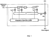
- FIG. 1 illustrates the signal flow of a typical LMS algorithm for the iterative adaptation of an exemplary FIR filter.
- An input signal x[n] is chosen as the reference signal for the adaptive LMS algorithm and the signal d[n] is taken as a second input signal.
- the signal d[n] is derived from input signal x[n] by filtering with a transfer function of an unknown system which is superimposed by background noise and apt to be approximated by the adaptive filter.
- These input signals may be acoustic signals which are converted into electric signals by means of microphones, for example. Likewise, however, these input signals may be or include electric signals that are generated by sensors for accommodating mechanical vibrations or also by revolution counters.
- FIG. 1 also shows a FIR filter of N-th order with which the input signal x[n] is converted into the signal y[n] over discrete time n.
- the N coefficients of the filter are identified with b 0 [n], b 1 [n] ... b N [n].
- the adaptation algorithm iteratively changes the filter coefficients b 0 [n], b 1 [n] ... b N [n] until an error signal e[n] which is the difference signal between the signal d[n] and the filtered input signal y[n] (output signal) is minimal.
- the signal d[n] is the input signal x[n] distorted by the unknown system which, in addition also includes background noise, if present.
- both of the signals x[n] and d[n] input into the adaptive filter are stochastic signals. In case of an acoustic echo cancellation system, they are noisy measuring signals, audio signals or communications signals, for example.
- the quality criterion expressed by the MSE can be minimized by means of a simple recursive algorithm, such as the known least mean square (LMS) algorithm.
- LMS least mean square
- the function to be minimized is the square of the error. That is, to determine an improved approximation for the minimum of the error square, only the error itself, multiplied with a constant, must be added to the last previously-determined approximation.
- the adaptive FIR filter must thereby be chosen to be at least as long as the relevant portion of the unknown impulse response of the unknown system to be approached, so that the adaptive filter has sufficient degrees of freedom to actually minimize the error signal e[n].
- the filter coefficients are gradually changed in the direction of the greatest decrease of the error margin MSE and in the direction of the negative gradient of the error margin MSE, respectively, wherein the parameter ⁇ controls the step size.
- the new filter coefficients b k [n+1] correspond to previous filter coefficients b k [n] plus a correction term, which is a function of the error signal e[n] and of the input signal vector x[n-k], which is assigned to the respective filter coefficient vector b k .
- the LMS convergence parameter ⁇ thereby represents a measure for the speed and for the stability of the adaptation of the filter.
- the least mean square algorithm of the adaptive LMS filter may thus be realized as outlined below.
- FIG. 2 shows a signal diagram of a method for estimation of the power spectral density of background noise using smoothing filtering but not voice detection.
- FIG. 2 shows an initial comparator step 1 and a second comparator step 4 as well as an initial calculation step 2 for computing the increase in the estimation of the power spectral density and a second calculation step 3 for computing the drop in the estimation of the power spectral density.
- a signal Noise[n] which may be the signal of a microphone measuring the background noise or the error signal of an adaptive filter (see FIG. 1 ), is compared in the comparator step 1 with the estimate NoiseLevel[n] of the estimated power spectral density computed in a previous step of the algorithm. If the current estimate value, Noise[n], is greater than the estimate NoiseLevel[n] of the estimated power spectral density computed in the previous step of the algorithm ("yes" path of step 1), a fixed predefined increment value C_Inc is added to the estimate NoiseLevel[n] computed in the previous step of the algorithm to produce a new, higher value NoiseLevel[n+1] for estimation of the power spectral density.
- the increment value C_Inc is constant and its value is independent on the amount the current value Noise[n]. This approach prevents any voice signals that may exist in the current value Noise[n], which typically have faster rises in level than the broadband background noise in the interior of an automobile, from significantly affecting the algorithm and consequently the computation of the estimate value.
- the decrement value C_Dec is constant and its value is independent of the amount the current value Noise[n]. This has the consequence that for both cases, i.e. for the increment or the decrement case, the estimated difference, in the rate of change of the level of the Noise[n] signal, is ignored.
- the newly computed estimate NoiseLevel[n+1] is compared in the step 4 with a fixed predefined minimum value MinNoiseLevel.
- the value of the newly computed estimate value NoiseLevel[n+1] is replaced by the value of the fixed predefined minimum value MinNoiseLevel - in other words, the estimate value is limited to the minimum value MinNoiseLevel.
- the purpose of this fixed predefined minimum value MinNoiseLevel is to prevent the NoiseLevel[n+1] signal from falling below this specified threshold value even if the Noise[n] signal is actually lower. In this way, the algorithm does not respond too slowly even for subsequent fast, strong rises in the Noise[n] signal.
- the disadvantage of said method can be that - both for the incrementing and decrementing of the estimate value of the power spectral density - the rate of change in level of the Noise[n] signal cannot be sufficiently approximated by the estimate value if the change in level of the background noise, for example, rises over a lengthy period (i.e., over several computation cycles of the algorithm in the same direction) and the rise in level of the Noise[n] signal for each computation cycle is considerably larger than the fixed increment C_Inc, which defines the maximum rise in level of the estimate value of the power spectral density in any given calculation step.
- the algorithm additionally is suitable only for estimating the overall level of the background noise throughout the entire frequency range that is observed.
- an appropriate frequency resolution of the estimated power spectral density is required for a suitable application of the estimate value of the power spectral density for noise suppression by filtering the signal.
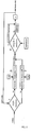
- FIG. 3 is a signal flow chart of a novel system to estimate the power spectral density of background noise without using voice detection.
- the system and method illustrated in FIG. 3 is, e.g., implemented using a digital signal processor.
- the system of FIG. 3 shows a power spectral density calculation unit 6, a time domain signal smoothing unit 7, a frequency domain signal smoothing unit 8, an increment calculation unit 9, a decrement calculation unit 10 and an estimate signal smoothing unit 11.
- the power spectral density calculation unit 6 computes the power spectral density (PSD) from an input signal MIC( ⁇ ), which yields the output signal PsdMic( ⁇ ) representing the power spectral density of the input signal MIC( ⁇ ).
- PSD power spectral density
- the input signal may be, e.g., a microphone signal as shown here, or an error signal of an adaptive filter (see FIG. 1 ). Then, as shown in FIG. 3 , the signal PsdMic( ⁇ ) is smoothed in the time domain (smoothing over time) using the time domain signal smoothing unit 7.
- the smoothing in the time domain has two different smoothing time constants, i.e. ⁇ up and ⁇ Down .
- the first time constant ⁇ up is applied if the signal rises, i.e. if it has a positive gradient - in contrast to the time constant ⁇ Down which is applied if the signals decreases, i.e. if it has a negative gradient.
- ⁇ up is applied if the signal rises, i.e. if it has a positive gradient - in contrast to the time constant ⁇ Down which is applied if the signals decreases, i.e. if it has a negative gradient.
- the main purpose of different up and down smoothing time constant is to address the sensitivity of human ears to rising or falling noise as they tend to be more sensitive to rising noise levels as to falling noise levels, provided, that both happen to have the same time constant.
- the output of the time domain signal smoothing unit 7 is smoothed in the frequency domain (smoothing over frequency) using the frequency domain signal smoothing unit 8.
- the frequencies f min and f max may be chosen such that a frequency range is included which covers the relevant frequency range of the acoustic perception in the human ear.
- the coefficients ⁇ up and ⁇ down for the smoothing of the PsdMic( ⁇ ) signal over frequency are selected in such a way that the greatest possible reduction in spectral fluctuations of the PsdMic( ⁇ ) signal is achieved to reduce the required computing power for the subsequent steps in the present method. At the same time this selection is made in a way that the necessary spectral information is retained so as to derive the frequency-dependent properties of the PsdMic( ⁇ ) signal relevant for perception by the human ear.
- the psychoacoustic evaluation steps (and units) to be considered here are shown further below.
- ⁇ up and ⁇ Down are chosen as equal values due to the fact that the main purpose of the up and down smoothing is to avoid frequency bias, which would occur if one would smooth in only one frequency direction. Hence, if one would smooth in the upward frequency direction with a different smoothing time constant as for the smoothing in the downward direction again a certain kind of frequency shift (bias) is created which originally was intended to be avoided by applying the up and down smoothing.
- the signal SmoothedPsdMic( ⁇ ) is obtained from the PsdMic( ⁇ ) signal through the smoothing in the time domain (smoothing over time, time domain signal smoothing unit 7) and in the frequency domain (smoothing over frequency, frequency domain signal smoothing unit 8).
- the SmoothedPsdMic( ⁇ ) signal is used as an input signal for the subsequent processing steps conducted in the increment calculation unit 9, the decrement calculation unit 10, and the estimate signal smoothing unit 11 in order to estimate the power spectral density of background noise without the use of a voice detection mechanism.
- the increment calculation unit 9 designates a calculation step for computing the relevant increments Inc( ⁇ ) for estimation of the power spectral density in the case of level rises in the SmoothedPsdMic( ⁇ ) signal for all spectral components of the smoothed signal SmoothedPsdMic( ⁇ ) to be considered.
- the decrement calculation unit 10 computes the relevant decrements Dec( ⁇ ) for estimation of the power spectral density in the case of decreasing levels in the SmoothedPsdMic( ⁇ ) signal for all spectral components of the smoothed signal SmoothedPsdMic( ⁇ ) to be considered.
- the estimate signal smoothing unit 11 refers to a memory less smoothing filtering step as shown in FIG. 2 , for which the increments and decrements for estimation of the rise or fall in level of the power spectral density are not specified as constants, but are adaptively dependent on the rate of rise or fall in the level.
- a current estimate value PsdNoise( ⁇ ) of the power spectral density is computed under consideration of a fixed minimum threshold PsdNoiseMin for each relevant spectral component of the smoothed signal SmoothedPsdMic( ⁇ ).
- the fixed minimum threshold PsdNoiseMin corresponds to the minimum value of the estimate value of the power spectral density shown in FIG. 2 as MinNoiseLevel.
- the disadvantage of known methods in the field is - for both incrementing and decrementing of the estimate value of the power spectral density - that the rate of change of level of the background noise cannot be adequately approximated by the estimate value in all cases. For example, this is the case if the change in level of the background noise rises over a lengthy period (i.e., over several computation cycles of the algorithm) and the rise in level of the background noise for each computation cycle of the algorithm is larger than the fixed increment, which defines the maximum rise in level of the estimate value of the power spectral density.
- the system of FIG. 3 for estimating the rise in level of the power spectral density in the case of rises in level of the background noise using an increment calculation unit 9 as shown in FIG. 3 eliminates this disadvantage without incurring a large, unwanted dependency on a voice signal present at the same time.
- Use is made of the fact that in particular the timing behavior differs considerably between voice signals and background noise. While voice signals typically exhibit fast rises and falls in level over time (speech dynamics), this is not generally the case for typical background noise signals, such as experienced in the interior of automobiles. Nevertheless, the known methods do not respond in particular cases fast enough to the changes in level of background noise typical for surrounding conditions, such as in automobiles.
- the increment calculation unit 9 shown in FIG. 3 to compute the increments of the estimate value of the power spectral density in response to rises in level of the background noise is illustrated in greater detail.
- a specified minimum value of the increment IncMin - for example, 0.5 dB per second - the new value of the increment Inc( ⁇ ) used in the computation of the estimate value is increased by a fixed value ⁇ Inc (for example, 0.01dB per frame, e.g., with a frame length e.g.
- a computation cycle may have, for example, a duration of 10 ms.
- the value of the increment Inc( ⁇ ) is continuously increased each time by 0.01 dB for each computation cycle of the algorithm in cases in which the value of the smoothed signal SmoothedPsdMic( ⁇ ) is continuously larger than the estimate value PsdNoise( ⁇ ) of the power spectral density computed in the previous computation cycle.
- the value of the smoothed signal SmoothedPsdMic( ⁇ ) obtained as the result of a new computation cycle is smaller than the estimate value PsdNoise( ⁇ ) of the power spectral density computed in the previous computation cycle, the value of the increment Inc( ⁇ ) is reset to the specified minimum value IncMin and the algorithm changes to the computation mode for determining the decrements for estimating the power spectral density for falling levels.
- the maximum possible value for the increment Inc( ⁇ ) is defined by the fixed predefined value IncMax - for example, 2.5 dB.
- the values of the decrement Dec( ⁇ ) for estimation of the value PsdNoise( ⁇ ) of the power spectral density of the background noise can also be computed for a decline in the level of the smoothed signal SmoothedPsdMic( ⁇ ).
- the estimate value PsdNoise( ⁇ ) of the power spectral density of the background noise is always reduced by the decrement Dec( ⁇ ) if the value of the smoothed signal SmoothedPsdMic( ⁇ ) is smaller than the estimate value PsdNoise( ⁇ ) of the power spectral density of the background noise computed in the previous computation cycle.
- a decrement calculation unit 10 is employed in this case.
- a specified value ⁇ Dec for adaptive adjustment of the decrement Dec( ⁇ ) is used.
- the new value of the decrement Dec( ⁇ ) used in the computation of the estimate value is increased by a fixed value ⁇ Dec (for example, 0.05 dB per frame e.g., with a frame length e.g.
- the value of the decrement Dec( ⁇ ) is increased continuously by 0.05 dB for each computation cycle of the algorithm in cases in which the value of the smoothed signal SmoothedPsdMic( ⁇ ) is continuously smaller than the estimate value PsdNoise( ⁇ ) of the power spectral density computed in the previous computation cycle.
- the value of the decrement Dec( ⁇ ) is reset to the specified minimum value DecMin and the algorithm changes to the computation mode to determine the increments for estimating the power spectral density for rising levels.
- the maximum possible value for the decrement Dec( ⁇ ) is likewise defined by the fixed predefined value DecMax - for example, 11 dB.
- the coefficients ⁇ up and ⁇ down mentioned earlier for smoothing over time and ⁇ up and ⁇ down for smoothing over frequency of the signal PsdMic( ⁇ ) can be determined, e.g., empirically from simulations and sample test circuits under different ambient conditions.
- the smoothing of the PsdMic( ⁇ ) signal in the frequency domain may be carried out twice with the calculated coefficients ⁇ up and ⁇ down - once in the direction from low to high frequencies, and once in the direction from high to low frequencies, whereby frequency shifts (bias) is avoided in the frequency representation of the signal.
- the coefficients ⁇ up and ⁇ down for smoothing over time and ⁇ up and ⁇ down for smoothing over frequency may be derived from the known psychoacoustic properties of the human ear in order to reduce the informational content of the smoothed signal SmoothedPsdMic( ⁇ ), i.e. the data rate.
- This is favorably to the extent that major benefits are obtained with regard to the smaller amount of computing power needed for the digital signal processor employed.
- Advantages can arise from a lesser dynamic level fluctuation of the smoothed signal SmoothedPsdMic( ⁇ ) in the time domain and a reduced number of spectral components in the frequency domain of the SmoothedPsdMic( ⁇ ) signal to be individually considered.
- a model can be created that indicates what acoustic signals or combinations of acoustic signals can be perceived or not by a human with undamaged hearing in the presence of noise signals, such as background noise.
- the threshold at which a test tone can just be perceived in the presence of a noisy signal is referred to as the masked threshold.
- the minimum audible threshold refers to the value at which a test tone can just be perceived in a fully quiet environment, where the area between the minimum audible threshold and a masked threshold caused by a masker, such as background noise, is known as the masking area.
- noise signals for example, the background noise in an automobile
- a psychoacoustic model considers the dependencies of the masking on the audio signal level, the spectral composition and the temporal characteristics.
- the basis for the modeling of the psychoacoustic masking is given by fundamental characteristics of the human ear, particularly the inner ear.
- the inner ear is located in the so-called petruous bone and filled with incompressible lymphatic fluid.
- the inner ear is shaped like a spiral (cochlea) with approximately 2 1 ⁇ 2 turns.
- the cochlea in turn comprises parallel canals, the upper and lower canals separated by the basilar membrane.
- the organ of Corti rests on the membrane and contains the sensory cells of the human ear. If the basilar membrane is made to vibrate by sound waves, nerve impulses are generated - i.e., no nodes or antinodes arise. This results in an effect that is crucial to hearing - the so-called frequency/location transformation on the basilar membrane, with which psychoacoustic masking effects and the refined frequency selectivity of the human ear can be explained.
- the human ear groups different sound waves that occur in limited frequency bands together so that they are processed as a single acoustic event. These frequency bands are known as critical frequency groups or as critical bandwidth (CB).
- CB critical frequency groups
- the basis of the CB is that the human ear compiles sounds in particular frequency bands as a common audible impression in regard to the psychoacoustic hearing impressions arising from the sound waves.
- Sonic activities that occur within a frequency group affect each other differently than sound waves occurring in different frequency groups. Two tones with the same level within one frequency group, for example, are perceived as being quieter than if they were in different frequency groups.
- the sought bandwidth of the frequency groups can be determined.
- the frequency groups In the case of low frequencies, the frequency groups have a bandwidth of 100 Hz. For frequencies above 500 Hz, the frequency groups have a bandwidth of about 20% of the center frequency of the corresponding frequency group.
- a hearing-oriented nonlinear frequency scale which is known as tonality and which has the unit "bark". It represents a distorted scaling of the frequency axis so that frequency groups have the same width of exactly 1 bark at every position.
- the nonlinear relationship between frequency and tonality is rooted in the frequency/location transformation on the basilar membrane.
- the tonality function was defined in tabular and equation form by Zwicker (see Zwicker, E.; Fastl, H.; Psychoacoustics - Facts and Models, 2nd edition, Springer-Verlag, Berlin/Heidelberg/New York, 1999 ) on the basis of masked threshold and loudness examinations.
- loudness and sound intensity refer to the same quantity of impression and differ only in their units. They consider the frequency-dependent perception of the human ear.
- the psychoacoustic dimension "loudness” indicates how loud a sound with a specific level, a specific spectral composition and a specific duration is subjectively perceived. The loudness becomes twice as large if a sound is perceived to be twice as loud, which allows different sound waves to be compared with each other in reference to the perceived loudness.
- the unit for evaluating and measuring loudness is a sone.
- One sone is defined as the perceived loudness of a tone having a loudness level of 40 phons - i.e., the perceived loudness of a tone that is perceived to have the same loudness as a sinus tone at a frequency of 1 kHz with a sound pressure level of 40 dB.
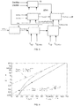
- FIG. 4 shows an example of the loudness N 1kHz of a stationary sinus tone with a frequency of 1 kHz and the loudness N GAR of a stationary uniform excitation noise in relation to the sound level - i.e., for signals for which time effects have no influence on the perceived loudness.
- Uniform excitation noise (GAR) is defined as a noise that has the same sound intensity in each frequency group and therefore the same excitation.
- FIG. 4 shows the loudness in sones in logarithmic scale versus sound pressure levels. For low sound pressure levels - i.e., when approaching the minimum audible threshold, the perceived loudness N of the tone falls dramatically.
- loudness N refers to the sound intensity of the emitted tone in watts per m 2
- I 0 refers to the reference sound intensity of 10 -12 watts per m 2 , which corresponds at medium frequencies to roughly the minimum audible threshold (see below).
- the loudness N is a useful means of determining masking by complex noise signals, and is thus a necessary requirement for a model of psychoacoustic masking through spectrally complex, time-dependent sounds.
- the so-called minimum audible threshold is obtained. Acoustic signals whose sound pressure levels are below the minimum audible threshold cannot be perceived by the human ear, even without the simultaneous presence of a noise signal.
- the so-called masked threshold is defined as the threshold of perception for a test sound in the presence of a noisy signal. If the test sound is below this psychoacoustic threshold, the test sound is fully masked. This means that all information within the psychoacoustic range of the masking cannot be perceived.
- Known compression and data reduction algorithms for audio signals also use this audio signal masking property, for example, to reduce information components in the signal under test without causing a perceivable deterioration in the quality of the actual signal.
- a known method is the ISO-MPEG audio compression process for layers 1, 2 and 3 devised by the Fraunhofer Institute for Integrated Circuits.
- Simultaneous masking means that a masking sound and useful signal occur at the same time. If the shape, bandwidth, amplitude and/or frequency of the masker changes in such a way that the frequently sinus-shaped test signals are just audible, the masked threshold can be determined for simultaneous masking throughout the entire bandwidth of the audible range - i.e., mainly for frequencies between 20 Hz and 20 kHz.
- FIG. 5 shows the masking of a sinusoidal test tone by white noise.
- the sound intensity of a test tone just masked by white noise with the sound intensity IWN is displayed in relation to its frequency.
- the minimum audible threshold is displayed as a dotted line.
- the minimum audible threshold of a sinus tone for masking by white noise is obtained as follows: below 500 Hz, the minimum audible threshold of the sinus tone is about 17 dB above the sound intensity of the white noise. Above 500 Hz the minimum audible threshold increases with about 10 dB per decade or about 3 dB per octave, corresponding to doubling the frequency.
- the frequency dependency of the minimum audible threshold is derived from the different critical bandwidth (CB) of the human ear at different center frequencies. Since the sound intensity occurring in a frequency group is compiled in the perceived audio impression, a greater overall intensity is obtained in wider frequency groups at high frequencies for white noise whose level is independent of frequency. The loudness of the sound also rises correspondingly (i.e., the perceived loudness) and causes increased masked thresholds.
- CB critical bandwidth
- the masked threshold is determined for narrowband maskers, such as sinus tones, narrowband noise or critical bandwidth noise, it is shown that the resulting spectral masked threshold is higher than the minimum audible threshold, even in areas in which the masker itself has no spectral components.
- Critical bandwidth noise is used in this case as narrowband noise, whose level is designated as L CB .
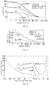
- FIG. 5 shows the masked thresholds of sinus tones measured as maskers due to critical bandwidth noise with a center frequency f c of 1 kHz, as well as of different sound pressure levels in relation to the frequency f T of the test tone with the level L T .
- the minimum audible threshold is shown by the dashed line in FIG. 5 .
- the peaks of the masked thresholds rise by 20 dB if the level of the masker also rises by 20 dB.
- the relationship is therefore linearly dependent on the level L CB of the masking critical bandwidth noise.
- the lower edge of the measured masked threshold i.e., the masking in the direction of low frequencies lower than the center frequency f c , has a gradient of about -100 dB/octave that is independent of the level L CB of the masked thresholds. This large gradient is only reached on the upper edge of the masked threshold for levels L CB of the masker that are lower than 40 dB.
- the upper edge of the masked threshold With increases in the level L CB of the masker, the upper edge of the masked threshold becomes flatter and flatter, and the gradient is about -25 dB/octave for an L CB of 100 dB. This means that the masking in the direction of higher frequencies compared to the center frequency f c of the masker extends far beyond the frequency range in which the masking sound is present. Hearing responds similarly for center frequencies other than 1 kHz for narrowband, critical bandwidth noise.
- the gradients of the upper and lower edges of the masked thresholds are practically independent of the center frequency of the masker - as seen in FIG. 7 .
- FIG. 7 shows the masked thresholds for maskers from critical bandwidth noise in the narrowband with a level L CB of 60 dB and three different center frequencies of 250 Hz, 1 kHz and 4 kHz.
- the apparently flatter flow of the gradient for the lower edge for the masker with the center frequency of 250 Hz is due to the minimum audible threshold, which applies at this low frequency even at higher levels. Effects such as those shown are likewise included in the implementation of a psychoacoustic model for the masking.
- the minimum audible threshold is again displayed in FIG. 7 by a dashed line.
- masked thresholds are obtained in relation to the frequency of the test tone and level of the masker L M as shown in FIG. 8 .
- the upper gradient is measured to be about -100 to -25 dB/octave in relation to the level of the masker, and about -100 dB/octave for the lower gradient.
- a difference of about 12 dB exists between the level L M of the masking tone and the maximum values of the masked thresholds L r .
- This difference is significantly greater than the value obtained with critical bandwidth noise as the masker. This is because the intensities of the two sinus tones of the masker and of the test tone are added together at the same frequency, unlike the use of noise and a sinus tone as the test tone. Consequently, the tone is perceived much earlier - i.e., for low levels for the test tone. Moreover, when emitting two sinus tones at the same time, other effects (such as beats) arise, which likewise lead to increased perception or reduced masking.
- the described simultaneous masking in the frequency domain has the effect that when smoothing in the frequency domain signal smoothing unit 8 (smoothing over frequency) only the spectral components of the PsdMic( ⁇ ) signal that are not masked by the critical bandwidth noise have to be considered.
- the algorithm can also be reduced for incrementing or decrementing the estimate value PsdNoise( ⁇ ) to the relevant spectral components and the masking characteristics caused and known by the components: a very significant reduction in the number of individual spectral components to be processed is therefore obtained if individual values for ⁇ Inc, ⁇ Dec, IncMin, DecMin, IncMax and DecMax are used.
- pre-masking refers to the situation in which masking effects occur already before the abrupt rise in the level of a masker.
- Post-masking describes the effect that occurs when the masked threshold does not immediately drop to the minimum audible threshold in the period after the fast fall in the level of a masker.
- FIG. 9 schematically shows both the pre- and post-masking, which are explained in greater detail further below in connection with the masking effect of tone impulses.
- test tone impulses of a short duration must be used to obtain the corresponding time resolution of the masking effects.
- the minimum audible threshold and masked threshold are both dependent on the duration of a test tone.
- Two different effects are known in this regard. These refer to the dependency of the loudness impression on the duration of a test impulse (see FIG. 10 ) and the relationship between the repetition rate of short tone impulses and loudness impression (see FIG. 11 ).
- the sound pressure level of a 20-ms impulse has to be increased by 10 dB in comparison to the sound pressure level of a 200-ms impulse in order to obtain the identical loudness impression.
- the loudness of a tone impulse is independent of its duration. It is known for the human ear that processes with a duration of more than about 200 ms represent stationary processes. Psychoacoustically certifiable effects of the timing properties of sounds exist if the sounds are shorter than about 200 ms.
- FIG. 10 shows the dependency of the perception of a test tone impulse on its duration.
- This behavior is independent of the frequency of the test tone, the absolute location of the lines for different frequencies f T of the test tone reflects the different minimum audible thresholds at these different frequencies.
- the continuous lines represent the masked thresholds for masking a test tone by uniform masking noise (UMN) with a level LUMN of 40 dB and 60 dB.
- Uniform masking noise is defined to be such that it has a constant masked threshold throughout the entire audible range - i.e., for all frequency groups from 0 to 24 barks.
- the displayed characteristics of the masked thresholds are independent of the frequency f T of the test tone.
- the masked thresholds also rise with about 10 dB per decade for durations of the test tone of less than 200 ms.
- FIG. 11 shows the dependency of the masked threshold on the repetition rate of a test tone impulse with the frequency 3 kHz and a duration of 3 ms.
- Uniform masking noise is again the masker: it is modulated with a rectangular shape - i.e., it is switched on and off periodically.
- the examined modulation frequencies of the uniform masking noise are 5 Hz, 20 Hz and 100 Hz.
- the test tone is emitted with a subsequent frequency identical to the modulation frequency of the uniform masking noise.
- the timing of the test tone impulses is correspondingly varied in order to obtain the time-related masked thresholds of the modulated noise.
- FIG. 11 shows the shift in time of the test tone impulse along the abscissa standardized to the period duration T M of the masker.
- the ordinate shows the level of the test tone impulse at the calculated masked threshold.
- the dashed line represents the masked threshold of the test tone impulse for an non modulated masker (i.e., continuously present masker with otherwise identical properties) as reference points.
- the flatter gradient of the post-masking in FIG. 11 in comparison to the gradient of the pre-masking is clear to see.
- the masked threshold is exceeded for a short period. This effect is known as an overshoot.
- the maximum drop ⁇ L in the level of the masked threshold for modulated uniform masking noise in the pauses of the masker is reduced as expected in comparison to the masked threshold for stationary uniform masking noise in response to an increase in the modulation frequency of the uniform masking noise - in other words, the masked threshold of the test tone impulse can fall less and less during its lifetime to the minimum value specified by the minimum audible threshold.
- FIG. 11 also illustrates that a masker already masks the test tone impulse before the masker is switched on at all.
- This effect is known - as already mentioned earlier - as pre-masking, and is based on the fact that loud tones and noises (i.e., with a high sound pressure level) can be processed more quickly by the hearing sense than quiet tones.
- the pre-masking effect is considerably less dominant than that of post-masking.
- the audible threshold does not fall immediately to the minimum audible threshold, but rather reaches it after a period of about 200 ms. The effect can be explained by the slow settling of the transient wave on the basilar membrane of the inner ear.
- the bandwidth of a masker also has direct influence on the duration of the post-masking. It is known that the particular components of a masker associated with each individual frequency group cause post-masking as shown in FIGS. 11 and 12 .
- FIG. 12 illustrates the level characteristics LT of the masked threshold of a Gaussian impulse with a duration of 20 ⁇ s as the test tone that is present at a time t v after the end of a rectangular-shaped masker consisting of white noise with a duration of 500 ms, where the sound pressure level LWR of the white noise takes on the three levels 40 dB, 60 dB and 80 dB.
- the post-masking of the masker comprising white noise can be measured without spectral effects, since the Gaussian-shaped test tone with a short duration of 20 ⁇ s in relation to the perceivable frequency range of the human ear also demonstrates a broadband spectral distribution similar to that of the white noise.
- the continuous curves in FIG. 12 illustrate the characteristic of the post processing determined by measurements.
- FIG. 12 shows curves by means of dotted lines that correspond to an exponential falling away of the post-masking with a time constant of 10 ms. It can be seen that a simple approximation of this kind can only hold true for large levels of the masker, and that it never reflects the characteristic of the post-masking in the vicinity of the minimum audible threshold.
- the psychoacoustic masking effects in algorithms and methods, such as the psychoacoustic masking model it also has to be known what resulting masking is obtained for grouped, complex or superimposed individual maskers.
- FIG. 13 shows the resulting masked thresholds for two cases in which all levels of the partial tones are either 40 dB or 60 dB.
- the fundamental tone and the first four harmonics are each located in separate frequency groups, meaning that there is no additive superimposition of the masking parts of these complex sound components for the maximum value of the masked threshold.
- FIG. 14 shows the simultaneous masking for a complex sound.
- the masked threshold for the simultaneous masking of a sinus-shaped test tone is represented by the 10 harmonics of a 200-Hz sinus tone in relation to the frequency and level of the excitation. All harmonics have the same sound pressure level, but their phase positions are statistically distributed.
- the known characteristics of the masked thresholds of sinus tones for masking by narrowband noise are used as the basis of the analysis.
- An example of this is the psychoacoustic core excitation of a sinus tone or a narrowband noise with a bandwidth smaller than the critical bandwidth matching the physical sound intensity. Otherwise, the signals are correspondingly distributed between the critical bandwidths masked by the audio spectrum.
- the distribution of the psychoacoustic excitation is obtained from the physical intensity spectrum of the received time-variable sound.
- the distribution of the psychoacoustic excitation is referred to as the specific loudness.
- the resulting overall loudness in the case of complex audio signals is found to be an integral over the specific loudness of all psychoacoustic excitations in the audible range along the tonal scale - i.e., in the range from 0 to 24 barks, and also exhibits corresponding time relations.
- the masked threshold is then created on the basis of the known relationship between loudness and masking, whereby the masked threshold drops to the minimum audible threshold in about 200 ms under consideration of time effects after termination of the sound within the relevant critical bandwidth (see also FIG. 12 , post-masking).
- the psychoacoustic masking model is implemented under consideration of all masking effects discussed above. It can be seen from the preceding FIGS. and explanations what masking effects are caused by sound pressure levels, spectral compositions and timing characteristics of noises, such as background noise, and how these effects can be utilized to reduce the information content of a signal using smoothing in the time and frequency domains without corrupting the resulting perceived impression. It is clear that a signal with less informational content in the time and frequency domains can be analyzed with highly reduced computing requirement in a digital signal processor in order to obtain an estimate of the power spectral density.
- the algorithm is also useful not to process the individual spectral components of the signal, but to compile the excitation patterns that occur in individual critical bandwidths or frequency groups.
- the basis of the critical bandwidth is that the human ear groups sounds together that arise in particular frequency ranges as a common aural impression regarding the psychoacoustic impressions of the sounds, where the scope of the aural impression can be covered by 24 successively arranged frequency groups.
- frequency groups can be defined in which no corruption is to be expected due to the simultaneous presence of voice signals.
- Other algorithms for example, simpler algorithms with fewer processing requirements
- filtering can be generally implemented for these sub bands without any previous estimation of the power spectral density.
- the frequency range of human speech typically extends from 60 Hz to 8 kHz, where the stated upper and lower limits are only reached in extreme cases and at very low levels.
- the stated methods and systems can be applied individually or in different combinations in accordance with the characteristics of the background noise and the general situation in order to obtain, on the one hand, the desired result - a reliable estimate of the power spectral density of the background noise without corruption by voice signals - and, on the other hand, to strongly minimize the required computing power for implementation on digital signal processors, so that costs can be saved.
- control time constants in the algorithm for estimating the power spectral density of the background noise.
- These control time constants increase the increments or decrements in increasing steps within defined maximum limits in the algorithm for approximation of the estimated power spectral density of the background noise to the actual level of the power spectral density of the background noise whenever the currently measured value of the power spectral density of the background noise continually exceeds or undershoots the estimate value of the power spectral density of the background noise in successive computational steps of the algorithm.
- the method does not derive the increments or decrements in the algorithm for approximation of the estimated power spectral density of the background noise to the actual level of the power spectral density of the background noise from the characteristic of the overall level of the power spectral density throughout the whole frequency domain. Rather the method refers to the individual spectral components of the power spectral density so that the different pattern of changes in level of the background noise is considered at various spectral positions.
- control time constants for the increments or decrements in the algorithm for approximation of the estimated power spectral density of the background noise are not determined for each individual spectral line in the power spectral density from the smoothed signal, but rather for a small number of frequency bands, which correspond to the frequency groups in which the human ear compiles sonic activity and, for example, uses for composing the perceived loudness, which consequently again requires considerably less computing power in comparison to the analysis of individual spectral components in the smoothed signal.
- This is achieved by merging all spectral components present in each one of consecutive frequency groups covering the frequency range of interest into a single combined signal representative for the spectral content of each of those frequency groups.
- the first and second coefficients for smoothing over time of the currently measured power spectral density may represent psychoacoustic sensory properties of the human ear
- the third and fourth coefficients for smoothing over frequency of the currently measured power spectral density may represent psychoacoustic sensory properties of the human ear.
- the value for the increase of the increment value may be individually selected with values differing for each spectral position in the (smoothed) power spectral density signal of the currently measured power spectral density and the value for the increase of the decrement value may be individually selected with values differing for each spectral position in the (smoothed power) spectral density signal of the currently measured power spectral density.
- Spectral components of the smoothed power spectral density signal may be merged within frequency groups corresponding to the psychoacoustic sensory perception into single combined signals for each frequency group prior to further processing.
Claims (14)
- System zum Schätzen der Leistungsspektraldichte von akustischem Hintergrundrauschen; wobei das System umfasst:eine Sensoreinheit zum Erhalten eines Rauschsignals (MIC (ω)), das das Hintergrundrauschen repräsentiert;eine Leistungsspektraldichte-Berechnungseinheit (6), die angepasst ist, die aktuelle Leistungsspektraldichte von dem Rauschsignal kontinuierlich zu bestimmen, und angepasst ist, ein entsprechendes Leistungsspektraldichte-Ausgabesignal (PsdMic (ω)) bereitzustellen;eine Zeitdomänen-Signalglättungseinheit (7), die angepasst ist, das Leistungsspektraldichte-Ausgabesignal (PsdMic (ω)) in der Zeitdomäne zu glätten, und angepasst ist, ein resultierendes zeitlich geglättetes Signal bereitzustellen;eine Frequenzdomänen-Signalglättungseinheit (8), die angepasst ist, das von der Zeitdomänen-Signalglättungseinheit (7) erhaltene zeitlich geglättete Signal in der Frequenzdomäne zu glätten, und angepasst ist, ein resultierendes geglättetes Leistungsspektraldichtesignal (SmoothedPsdMic (ω)) bereitzustellen;eine Zunahmeberechnungseinheit (9), die angepasst ist, eine Zunahme (Inc ((ω)) abhängig von einem geschätzten Wert der Leistungsspektraldichte des Hintergrundrauschen (PsdNoise (ω)) zu berechnen;eine Abnahmeberechnungseinheit (10), die angepasst ist, eine Abnahme (Dec (ω)) abhängig von einem geschätzten Wert der Leistungsspektraldichte des Hintergrundrauschen zu berechnen; undeine Glättungseinheit (11) für das geschätzte Signal, die angepasst ist, den geschätzten Wert der Leistungsspektraldichte des Hintergrundrauschens (PsdNoise (ω)) aus der Zunahme (Inc (ω)) und der Abnahme (Dec (ω)) zu berechnen; wobeider Zunahmewert (Inc (ω)), wenn der aktuell bestimmte Wert der geglätteten Leistungsspektraldichte (SmoothedPsdMic (ω)) in einem neuen Berechnungszyklus größer als der geschätzte Wert der Leistungsspektraldichte des Hintergrundrauschens (PsdNoise (ω)) ist, der in dem vorigen Berechnungszyklus bestimmt wurde, um eine vorbestimmte Menge (ΔInc) erhöht wird, wobei bei einem Minimum-Zunahmewert (Inc (ω)) gestartet wird, bis ein Maximum-Zunahmewert (IncMax) erreicht ist; undder Abnahmewert (Dec (ω)), wenn der aktuell bestimmte Wert der geglätteten Leistungsspektraldichte (SmoothedPsdMic (ω)) in einem neuen Berechnungszyklus kleiner als der geschätzte Wert der Leistungsspektraldichte des Hintergrundrauschens (PsdNoise (ω)) ist, der in dem vorigen Berechnungszyklus bestimmt wurde, um eine vorbestimmte Menge (ΔDec) erhöht wird, wobei bei einem Minimum-Abnahmewert (DecMin) gestartet wird, bis ein Maximum-Abnahmewert (DecMax) erreicht ist.
- System nach Anspruch 1, weiter umfassend ein adaptives Filter, das ein Fehlersignal (e[n]) bereitstellt, wobei die Leistungsspektraldichte-Berechnungseinheit (6) angepasst ist, die aktuelle Leistungsspektraldichte aus dem Fehlersignal (e[n]) des adaptiven Filters durch das Einsetzen von konsekutiven Berechnungszyklen zu bestimmen, und das System angepasst ist, ein entsprechendes Leistungsspektraldichte-Ausgabesignal (PsdMic(ω)) und ein entsprechendes geglättetes Leistungsspektraldichtesignal (SmoothedPsdMic(ω)) bereitzustellen.
- System nach Anspruch 1 oder 2, wobei das System angepasst ist, die Berechnung zum Schätzen der Leistungsspektraldichte des Hintergrundrauschens von dem Modus zum Berechnen des Zunahmewertes zu dem Modus zum Berechnen des Abnahmewertes zu wechseln, wenn der aktuelle bestimmte Wert der Leistungsspektraldichte in einem neuen Berechnungszyklus kleiner als der geschätzte Wert der Leistungsspektraldichte des Hintergrundrauschens ist, der in dem vorigen Zyklus berechnet wurde, wobei das System angepasst ist, den aktuellen Wert des Zunahmewerts auf den Minimum-Zunahmewert zurückzusetzen, und
die Berechnung zum Schätzen der Leistungsspektraldichte des Hintergrundrauschens von dem Modus zum Berechnen des Abnahmewertes zu dem Modus zum Berechnen des Zunahmewertes zu wechseln, wenn der aktuelle bestimmte Wert der Leistungsspektraldichte in einem neuen Berechnungszyklus größer als der geschätzte Wert der Leistungsspektraldichte des Hintergrundrauschens ist, der in dem vorigen Berechnungszyklus berechnet wurde, wobei das System angepasst ist, den aktuellen Wert des Abnahmewerts auf den Minimum-Abnahmewert zurückzusetzen. - System nach einem der Ansprüche 1-3, wobei das System in dem Fall der Abnahme des geschätzten Werts der Leistungsspektraldichte des Hintergrundrauschens angepasst ist, die Verminderung des geschätzten Wertes auf einen festen spezifizierten Wert zu begrenzen, sodass der geschätzte Wert der Leistungsspektraldichte des Hintergrundrauschens nie unter den Minimumwert fällt, unabhängig von dem aktuell berechneten Wert.
- System nach einem der Ansprüche 1-4, wobei die Zeitdomänen-Signalglättungseinheit angepasst ist, die aktuell gemessene Leistungsspektraldichte über einen Zeitraum zu glätten, indem zwei verschiedene Zeitkonstanten verwendet werden, eine für den Fall eines steigenden Signals und eine für den Fall eines fallenden Signals.
- System nach einem der Ansprüche 1-5, wobei die Frequenzdomänen-Signalglättungseinheit (8) angepasst ist, das zeitlich geglättete Signal von der Zeitdomänen-Signalglättungseinheit (7) zu glätten, wobei unter Verwendung eines dritten Frequenzglättungskoeffizienten von einer Minimumfrequenz nach oben gestartet wird, und/oder unter Verwendung eines vierten Frequenzglättungskoeffizienten von einer Maximumfrequenz nach unten gestartet wird.
- System nach einem der Ansprüche 1-6, wobei der Wert (ΔInc) für die Erhöhung des Zunahmewerts individuell ausgewählt wird mit Werten, die für jede Spektralposition in dem geglätteten Leistungsspektraldichtewert der aktuell gemessenen Leistungsspektraldichte verschieden sind, und wobei der Wert (ΔDec) für die Erhöhung des Abnahmewerts individuell ausgewählt wird mit Werten, die für jede Spektralposition in dem geglätteten Leistungsspektraldichtewert der aktuell gemessenen Leistungsspektraldichte verschieden sind.
- System nach einem der Ansprüche 1-7, wobei das System angepasst ist, vor dem weiteren Verarbeiten spektrale Komponenten des geglätteten oder ungeglätteten Leistungsspektraldichtesignals innerhalb von Frequenzgruppen, die der psychoakustischen Sinneswahrnehmung entsprechen, in einzelne kombinierte Signale für jede Frequenzgruppe zu vereinen.
- Verfahren zum Bestimmen der Leistungsspektraldichte von akustischem Hintergrundrauschen, umfassend die Schritte des:Bestimmens der aktuellen Leistungsspektraldichte von einem Mikrofonsignal (MIC(ω)) durch eine Leistungsspektraldichten-Berechnungseinheit (6) und Bereitstellens eines entsprechenden Leistungsspektraldichte-Ausgabesignals (PsdMic(ω));Glättens des bereitgestellten Leistungsspektraldichte-Ausgabesignals (PsdMic(ω)) in der Zeitdomäne, indem ein resultierendes zeitlich geglättetes Signal bereitgestellt wird;Glättens des zeitlich geglätteten Signals in der Frequenzdomäne und Bereitstellens eines resultierenden geglätteten Leistungsspektraldichte-Ausgabesignals (SmoothedPsdMic(ω));Berechnens einer Zunahme (Inc ((ω)), abhängig von einem geschätzten Wert einer Leistungsspektraldichte des Hintergrundrauschen;Berechnens einer Abnahme (Dec ((ω)), abhängig von dem geschätzten Wert der Leistungsspektraldichte des Hintergrundrauschen;Berechnens des geschätzten Werts der Leistungsspektraldichte des Hintergrundrauschens aus der Zunahme und der Abnahme,
wobeider Zunahmewert (Inc (ω)), wenn der aktuell bestimmte Wert der geglätteten Leistungsspektraldichte (SmoothedPsdMic (ω)) in einem neuen Berechnungszyklus größer als der geschätzte Wert der Leistungsspektraldichte des Hintergrundrauschens (PsdNoise (ω)) ist, der in dem vorigen Berechnungszyklus bestimmt wurde, um eine vorbestimmte Menge (ΔInc) erhöht wird, wobei bei einem Minimum-Zunahmewert (Inc (ω) gestartet wird, bis ein Maximum-Zunahmewert (IncMax) erreicht ist, undder Abnahmewert (Dec (ω)), wenn der aktuell bestimmte Wert der geglätteten Leistungsspektraldichte (SmoothedPsdMic (ω)) in einem neuen Berechnungszyklus kleiner als der geschätzte Wert der Leistungsspektraldichte des Hintergrundrauschens (PsdNoise (ω)) ist, der in dem vorigen Berechnungszyklus bestimmt wurde, um eine vorbestimmte Menge (ΔDec) erhöht wird, wobei bei einem Minimum-Abnahmewert (DecMin) gestartet wird, bis ein Maximum-Abnahmewert (DecMax) erreicht ist. - Verfahren nach Anspruch 9, ferner umfassend den Schritt des:Bestimmens der aktuellen Leistungsspektraldichte aus einem Fehlersignal, das von adaptivem Filtern durch das Einsetzen konsekutiver Berechnungszyklen abgeleitet wurde; undBereitstellens eines entsprechenden Leistungsspektraldichte-Ausgabesignals (PsdMic(ω)) und eines entsprechenden geglätteten Leistungsspektraldichte-Ausgabesignals (SmoothedPsdMic(ω)).
- Verfahren nach Anspruch 9 oder 10, ferner umfassend die Schritte des:Wechselns der Berechnung zum Schätzen der Leistungsspektraldichte des Hintergrundrauschens von dem Modus zum Berechnen des Zunahmewertes zu dem Modus zum Berechnen des Abnahmewertes, wenn der aktuelle bestimmte Wert der Leistungsspektraldichte in einem neuen Berechnungszyklus kleiner als der geschätzte Wert der Leistungsspektraldichte des Hintergrundrauschens ist, der in dem vorigen Berechnungszyklus berechnet wurde, wobei der aktuelle Wert des Zunahmewerts (Inc (ω)) auf den Minimum-Zunahmewert (IncMin) zurückgesetzt wird, undWechselns der Berechnung zum Schätzen der Leistungsspektraldichte des Hintergrundrauschens von dem Modus zum Berechnen des Abnahmewertes zu dem Modus zum Berechnen des Zunahmewertes, wenn der aktuelle bestimmte Wert der Leistungsspektraldichte in einem neuen Berechnungszyklus größer als der geschätzte Wert der Leistungsspektraldichte des Hintergrundrauschens ist, der in dem vorigen Berechnungszyklus berechnet wurde, wobei der aktuelle Wert des Abnahmewerts (Dec (ω)) auf den Minimum-Abnahmewert (DecMin) zurückgesetzt wird.
- Verfahren nach einem der Ansprüche 9-11, ferner umfassend den Schritt des Begrenzens der Verminderung des geschätzten Wertes auf einen festen spezifizierten Wert, in dem Fall der Abnahme des geschätzten Werts der Leistungsspektraldichte des Hintergrundrauschens, sodass der geschätzte Wert der Leistungsspektraldichte des Hintergrundrauschens nie unter den Minimumwert fällt, unabhängig von dem aktuell berechneten Wert.
- Verfahren nach einem der Ansprüche 9-12, ferner umfassend den Schritt des Glättens der aktuell gemessenen Leistungsspektraldichte in der Zeitdomäne über einen Zeitraum, indem zwei verschiedene Zeitkonstanten verwendet werden, eine für den Fall eines steigenden Signals und eine für den Fall eines fallenden Signals.
- Verfahren nach einem der Ansprüche 9-13, ferner umfassend den Schritt des Glättens des zeitlich geglätteten Signals von der Zeitdomänen-Signalglättungseinheit (7) in der Frequenzdomäne, wobei unter Verwendung eines dritten Frequenzglättungskoeffizienten von einer Minimumfrequenz nach oben gestartet wird, und/oder unter Verwendung eines vierten Frequenzglättungskoeffizienten von einer Maximumfrequenz nach unten gestartet wird.
Priority Applications (3)
| Application Number | Priority Date | Filing Date | Title |
|---|---|---|---|
| EP09154541.8A EP2226794B1 (de) | 2009-03-06 | 2009-03-06 | Hintergrundgeräuschschätzung |
| JP2010012611A JP5439200B2 (ja) | 2009-03-06 | 2010-01-22 | バックグラウンドノイズ推定 |
| US12/718,473 US8422697B2 (en) | 2009-03-06 | 2010-03-05 | Background noise estimation |
Applications Claiming Priority (1)
| Application Number | Priority Date | Filing Date | Title |
|---|---|---|---|
| EP09154541.8A EP2226794B1 (de) | 2009-03-06 | 2009-03-06 | Hintergrundgeräuschschätzung |
Related Child Applications (1)
| Application Number | Title | Priority Date | Filing Date |
|---|---|---|---|
| EP16203829.3 Division-Into | 2016-12-13 |
Publications (2)
| Publication Number | Publication Date |
|---|---|
| EP2226794A1 EP2226794A1 (de) | 2010-09-08 |
| EP2226794B1 true EP2226794B1 (de) | 2017-11-08 |
Family
ID=40910903
Family Applications (1)
| Application Number | Title | Priority Date | Filing Date |
|---|---|---|---|
| EP09154541.8A Active EP2226794B1 (de) | 2009-03-06 | 2009-03-06 | Hintergrundgeräuschschätzung |
Country Status (3)
| Country | Link |
|---|---|
| US (1) | US8422697B2 (de) |
| EP (1) | EP2226794B1 (de) |
| JP (1) | JP5439200B2 (de) |
Families Citing this family (19)
| Publication number | Priority date | Publication date | Assignee | Title |
|---|---|---|---|---|
| US9589580B2 (en) * | 2011-03-14 | 2017-03-07 | Cochlear Limited | Sound processing based on a confidence measure |
| US9516371B2 (en) | 2012-04-24 | 2016-12-06 | Mobitv, Inc. | Closed captioning management system |
| US9135920B2 (en) * | 2012-11-26 | 2015-09-15 | Harman International Industries, Incorporated | System for perceived enhancement and restoration of compressed audio signals |
| DE102013111784B4 (de) | 2013-10-25 | 2019-11-14 | Intel IP Corporation | Audioverarbeitungsvorrichtungen und audioverarbeitungsverfahren |
| WO2015129760A1 (ja) * | 2014-02-28 | 2015-09-03 | 日本電信電話株式会社 | 信号処理装置、方法及びプログラム |
| EP2980798A1 (de) | 2014-07-28 | 2016-02-03 | Fraunhofer-Gesellschaft zur Förderung der angewandten Forschung e.V. | Harmonizitätsabhängige Steuerung eines harmonischen Filterwerkzeugs |
| AT516046B1 (de) * | 2014-12-30 | 2016-02-15 | Audio Lab Swiss Ag | Verfahren und vorrichtung zur bestimmung der qualität eines übertragungssystems |
| EP3252769B8 (de) * | 2016-06-03 | 2020-04-01 | Sony Corporation | Hinzufügung von hintergrundgeräuschen zu audiodaten mit sprachinhalt |
| SE541331C2 (en) | 2017-11-30 | 2019-07-09 | Creo Dynamics Ab | Active noise control method and system |
| SE1850077A1 (en) | 2018-01-24 | 2019-07-25 | Creo Dynamics Ab | Active noise control method and system using variable actuator and sensor participation |
| CN108922556B (zh) * | 2018-07-16 | 2019-08-27 | 百度在线网络技术(北京)有限公司 | 声音处理方法、装置及设备 |
| CN109643554B (zh) * | 2018-11-28 | 2023-07-21 | 深圳市汇顶科技股份有限公司 | 自适应语音增强方法和电子设备 |
| CN109727605B (zh) * | 2018-12-29 | 2020-06-12 | 苏州思必驰信息科技有限公司 | 处理声音信号的方法及系统 |
| CN110031083A (zh) * | 2018-12-31 | 2019-07-19 | 瑞声科技(新加坡)有限公司 | 一种噪音总声压级测量方法、系统及计算机可读存储介质 |
| CN110021305B (zh) * | 2019-01-16 | 2021-08-20 | 上海惠芽信息技术有限公司 | 一种音频滤波方法、音频滤波装置及可穿戴设备 |
| US11011182B2 (en) * | 2019-03-25 | 2021-05-18 | Nxp B.V. | Audio processing system for speech enhancement |
| CN112133322A (zh) * | 2020-10-19 | 2020-12-25 | 南通赛洋电子有限公司 | 一种基于噪声分类优化imcra算法的语音增强方法 |
| CN113808607A (zh) * | 2021-03-05 | 2021-12-17 | 北京沃东天骏信息技术有限公司 | 基于神经网络的语音增强方法、装置及电子设备 |
| CN113008364B (zh) * | 2021-04-05 | 2022-07-15 | 中国人民解放军63966部队 | 装甲车辆隐蔽性噪声测量方法和装置 |
Citations (1)
| Publication number | Priority date | Publication date | Assignee | Title |
|---|---|---|---|---|
| US6263307B1 (en) * | 1995-04-19 | 2001-07-17 | Texas Instruments Incorporated | Adaptive weiner filtering using line spectral frequencies |
Family Cites Families (5)
| Publication number | Priority date | Publication date | Assignee | Title |
|---|---|---|---|---|
| DE69229627T2 (de) * | 1991-03-05 | 1999-12-02 | Picturetel Corp | Sprachkodierer mit veränderlicher bitrate |
| JPH08506434A (ja) * | 1993-11-30 | 1996-07-09 | エイ・ティ・アンド・ティ・コーポレーション | 通信システムにおける伝送ノイズ低減 |
| US7177805B1 (en) * | 1999-02-01 | 2007-02-13 | Texas Instruments Incorporated | Simplified noise suppression circuit |
| US7454332B2 (en) * | 2004-06-15 | 2008-11-18 | Microsoft Corporation | Gain constrained noise suppression |
| DE602006005684D1 (de) | 2006-10-31 | 2009-04-23 | Harman Becker Automotive Sys | Modellbasierte Verbesserung von Sprachsignalen |
-
2009
- 2009-03-06 EP EP09154541.8A patent/EP2226794B1/de active Active
-
2010
- 2010-01-22 JP JP2010012611A patent/JP5439200B2/ja active Active
- 2010-03-05 US US12/718,473 patent/US8422697B2/en active Active
Patent Citations (1)
| Publication number | Priority date | Publication date | Assignee | Title |
|---|---|---|---|---|
| US6263307B1 (en) * | 1995-04-19 | 2001-07-17 | Texas Instruments Incorporated | Adaptive weiner filtering using line spectral frequencies |
Also Published As
| Publication number | Publication date |
|---|---|
| US8422697B2 (en) | 2013-04-16 |
| JP2010211190A (ja) | 2010-09-24 |
| US20100226501A1 (en) | 2010-09-09 |
| EP2226794A1 (de) | 2010-09-08 |
| JP5439200B2 (ja) | 2014-03-12 |
Similar Documents
| Publication | Publication Date | Title |
|---|---|---|
| EP2226794B1 (de) | Hintergrundgeräuschschätzung | |
| EP1947642B1 (de) | Aktives geräuschdämpfungssystem | |
| EP2056296B1 (de) | Dynamische Geräuschunterdrückung | |
| EP1450353B1 (de) | Vorrichtung zur Unterdrückung von Windgeräuschen | |
| US7454010B1 (en) | Noise reduction and comfort noise gain control using bark band weiner filter and linear attenuation | |
| US8976974B2 (en) | Sound tuning system | |
| EP2629294B1 (de) | System und Verfahren für dynamische Restgeräuschformung | |
| US8364479B2 (en) | System for speech signal enhancement in a noisy environment through corrective adjustment of spectral noise power density estimations | |
| EP2234105B1 (de) | Hintergrundgeräuschschätzung | |
| US20050288923A1 (en) | Speech enhancement by noise masking | |
| JP2008537185A (ja) | オーディオ雑音を減少させるシステムおよび方法 | |
| US6510408B1 (en) | Method of noise reduction in speech signals and an apparatus for performing the method | |
| WO2004086362A1 (ja) | 音声信号雑音除去装置、音声信号雑音除去方法及びプログラム | |
| EP1995722B1 (de) | Verfahren zur Verarbeitung eines akustischen Eingangssignals zweck Sendung eines Ausgangssignals mit reduzierter Lautstärke | |
| EP2230664B1 (de) | Verfahren und Vorrichtung zur Dämpfung von Rauschen in einem Eingangssignal | |
| EP2490218A1 (de) | Verfahren zur Interferenzunterdrückung | |
| Pinto et al. | Adaptive audio equalization of rooms based on a technique of transparent insertion of acoustic probe signals | |
| Upadhyay et al. | A perceptually motivated stationary wavelet packet filter-bank utilizing improved spectral over-subtraction algorithm for enhancing speech in non-stationary environments | |
| CN117714956A (zh) | 确定听力仪器的声学特性 |
Legal Events
| Date | Code | Title | Description |
|---|---|---|---|
| PUAI | Public reference made under article 153(3) epc to a published international application that has entered the european phase |
Free format text: ORIGINAL CODE: 0009012 |
|
| 17P | Request for examination filed |
Effective date: 20090904 |
|
| AK | Designated contracting states |
Kind code of ref document: A1 Designated state(s): AT BE BG CH CY CZ DE DK EE ES FI FR GB GR HR HU IE IS IT LI LT LU LV MC MK MT NL NO PL PT RO SE SI SK TR |
|
| AX | Request for extension of the european patent |
Extension state: AL BA RS |
|
| AKX | Designation fees paid |
Designated state(s): AT BE BG CH CY CZ DE DK EE ES FI FR GB GR HR HU IE IS IT LI LT LU LV MC MK MT NL NO PL PT RO SE SI SK TR |
|
| APBK | Appeal reference recorded |
Free format text: ORIGINAL CODE: EPIDOSNREFNE |
|
| APBN | Date of receipt of notice of appeal recorded |
Free format text: ORIGINAL CODE: EPIDOSNNOA2E |
|
| APBR | Date of receipt of statement of grounds of appeal recorded |
Free format text: ORIGINAL CODE: EPIDOSNNOA3E |
|
| APAF | Appeal reference modified |
Free format text: ORIGINAL CODE: EPIDOSCREFNE |
|
| APBT | Appeal procedure closed |
Free format text: ORIGINAL CODE: EPIDOSNNOA9E |
|
| REG | Reference to a national code |
Ref country code: DE Ref legal event code: R079 Ref document number: 602009049222 Country of ref document: DE Free format text: PREVIOUS MAIN CLASS: G10L0021020000 Ipc: G10L0021020800 |
|
| GRAP | Despatch of communication of intention to grant a patent |
Free format text: ORIGINAL CODE: EPIDOSNIGR1 |
|
| RIC1 | Information provided on ipc code assigned before grant |
Ipc: G10L 21/0216 20130101ALN20170517BHEP Ipc: G10L 21/0208 20130101AFI20170517BHEP |
|
| RIC1 | Information provided on ipc code assigned before grant |
Ipc: G10L 21/0216 20130101ALN20170522BHEP Ipc: G10L 21/0208 20130101AFI20170522BHEP |
|
| INTG | Intention to grant announced |
Effective date: 20170606 |
|
| GRAS | Grant fee paid |
Free format text: ORIGINAL CODE: EPIDOSNIGR3 |
|
| GRAA | (expected) grant |
Free format text: ORIGINAL CODE: 0009210 |
|
| AK | Designated contracting states |
Kind code of ref document: B1 Designated state(s): AT BE BG CH CY CZ DE DK EE ES FI FR GB GR HR HU IE IS IT LI LT LU LV MC MK MT NL NO PL PT RO SE SI SK TR |
|
| REG | Reference to a national code |
Ref country code: GB Ref legal event code: FG4D |
|
| REG | Reference to a national code |
Ref country code: CH Ref legal event code: EP Ref country code: AT Ref legal event code: REF Ref document number: 944866 Country of ref document: AT Kind code of ref document: T Effective date: 20171115 |
|
| REG | Reference to a national code |
Ref country code: IE Ref legal event code: FG4D |
|
| REG | Reference to a national code |
Ref country code: DE Ref legal event code: R096 Ref document number: 602009049222 Country of ref document: DE |
|
| REG | Reference to a national code |
Ref country code: NL Ref legal event code: MP Effective date: 20171108 |
|
| REG | Reference to a national code |
Ref country code: LT Ref legal event code: MG4D |
|
| REG | Reference to a national code |
Ref country code: AT Ref legal event code: MK05 Ref document number: 944866 Country of ref document: AT Kind code of ref document: T Effective date: 20171108 |
|
| PG25 | Lapsed in a contracting state [announced via postgrant information from national office to epo] |
Ref country code: NL Free format text: LAPSE BECAUSE OF FAILURE TO SUBMIT A TRANSLATION OF THE DESCRIPTION OR TO PAY THE FEE WITHIN THE PRESCRIBED TIME-LIMIT Effective date: 20171108 Ref country code: LT Free format text: LAPSE BECAUSE OF FAILURE TO SUBMIT A TRANSLATION OF THE DESCRIPTION OR TO PAY THE FEE WITHIN THE PRESCRIBED TIME-LIMIT Effective date: 20171108 Ref country code: ES Free format text: LAPSE BECAUSE OF FAILURE TO SUBMIT A TRANSLATION OF THE DESCRIPTION OR TO PAY THE FEE WITHIN THE PRESCRIBED TIME-LIMIT Effective date: 20171108 Ref country code: NO Free format text: LAPSE BECAUSE OF FAILURE TO SUBMIT A TRANSLATION OF THE DESCRIPTION OR TO PAY THE FEE WITHIN THE PRESCRIBED TIME-LIMIT Effective date: 20180208 Ref country code: SE Free format text: LAPSE BECAUSE OF FAILURE TO SUBMIT A TRANSLATION OF THE DESCRIPTION OR TO PAY THE FEE WITHIN THE PRESCRIBED TIME-LIMIT Effective date: 20171108 Ref country code: FI Free format text: LAPSE BECAUSE OF FAILURE TO SUBMIT A TRANSLATION OF THE DESCRIPTION OR TO PAY THE FEE WITHIN THE PRESCRIBED TIME-LIMIT Effective date: 20171108 |
|
| PG25 | Lapsed in a contracting state [announced via postgrant information from national office to epo] |
Ref country code: HR Free format text: LAPSE BECAUSE OF FAILURE TO SUBMIT A TRANSLATION OF THE DESCRIPTION OR TO PAY THE FEE WITHIN THE PRESCRIBED TIME-LIMIT Effective date: 20171108 Ref country code: GR Free format text: LAPSE BECAUSE OF FAILURE TO SUBMIT A TRANSLATION OF THE DESCRIPTION OR TO PAY THE FEE WITHIN THE PRESCRIBED TIME-LIMIT Effective date: 20180209 Ref country code: AT Free format text: LAPSE BECAUSE OF FAILURE TO SUBMIT A TRANSLATION OF THE DESCRIPTION OR TO PAY THE FEE WITHIN THE PRESCRIBED TIME-LIMIT Effective date: 20171108 Ref country code: BG Free format text: LAPSE BECAUSE OF FAILURE TO SUBMIT A TRANSLATION OF THE DESCRIPTION OR TO PAY THE FEE WITHIN THE PRESCRIBED TIME-LIMIT Effective date: 20180208 Ref country code: IS Free format text: LAPSE BECAUSE OF FAILURE TO SUBMIT A TRANSLATION OF THE DESCRIPTION OR TO PAY THE FEE WITHIN THE PRESCRIBED TIME-LIMIT Effective date: 20180308 Ref country code: LV Free format text: LAPSE BECAUSE OF FAILURE TO SUBMIT A TRANSLATION OF THE DESCRIPTION OR TO PAY THE FEE WITHIN THE PRESCRIBED TIME-LIMIT Effective date: 20171108 |
|
| PG25 | Lapsed in a contracting state [announced via postgrant information from national office to epo] |
Ref country code: DK Free format text: LAPSE BECAUSE OF FAILURE TO SUBMIT A TRANSLATION OF THE DESCRIPTION OR TO PAY THE FEE WITHIN THE PRESCRIBED TIME-LIMIT Effective date: 20171108 Ref country code: EE Free format text: LAPSE BECAUSE OF FAILURE TO SUBMIT A TRANSLATION OF THE DESCRIPTION OR TO PAY THE FEE WITHIN THE PRESCRIBED TIME-LIMIT Effective date: 20171108 Ref country code: CZ Free format text: LAPSE BECAUSE OF FAILURE TO SUBMIT A TRANSLATION OF THE DESCRIPTION OR TO PAY THE FEE WITHIN THE PRESCRIBED TIME-LIMIT Effective date: 20171108 Ref country code: CY Free format text: LAPSE BECAUSE OF FAILURE TO SUBMIT A TRANSLATION OF THE DESCRIPTION OR TO PAY THE FEE WITHIN THE PRESCRIBED TIME-LIMIT Effective date: 20171108 Ref country code: SK Free format text: LAPSE BECAUSE OF FAILURE TO SUBMIT A TRANSLATION OF THE DESCRIPTION OR TO PAY THE FEE WITHIN THE PRESCRIBED TIME-LIMIT Effective date: 20171108 |
|
| REG | Reference to a national code |
Ref country code: DE Ref legal event code: R097 Ref document number: 602009049222 Country of ref document: DE |
|
| PG25 | Lapsed in a contracting state [announced via postgrant information from national office to epo] |
Ref country code: RO Free format text: LAPSE BECAUSE OF FAILURE TO SUBMIT A TRANSLATION OF THE DESCRIPTION OR TO PAY THE FEE WITHIN THE PRESCRIBED TIME-LIMIT Effective date: 20171108 Ref country code: IT Free format text: LAPSE BECAUSE OF FAILURE TO SUBMIT A TRANSLATION OF THE DESCRIPTION OR TO PAY THE FEE WITHIN THE PRESCRIBED TIME-LIMIT Effective date: 20171108 Ref country code: PL Free format text: LAPSE BECAUSE OF FAILURE TO SUBMIT A TRANSLATION OF THE DESCRIPTION OR TO PAY THE FEE WITHIN THE PRESCRIBED TIME-LIMIT Effective date: 20171108 |
|
| PLBE | No opposition filed within time limit |
Free format text: ORIGINAL CODE: 0009261 |
|
| STAA | Information on the status of an ep patent application or granted ep patent |
Free format text: STATUS: NO OPPOSITION FILED WITHIN TIME LIMIT |
|
| 26N | No opposition filed |
Effective date: 20180809 |
|
| REG | Reference to a national code |
Ref country code: CH Ref legal event code: PL |
|
| PG25 | Lapsed in a contracting state [announced via postgrant information from national office to epo] |
Ref country code: SI Free format text: LAPSE BECAUSE OF FAILURE TO SUBMIT A TRANSLATION OF THE DESCRIPTION OR TO PAY THE FEE WITHIN THE PRESCRIBED TIME-LIMIT Effective date: 20171108 Ref country code: MC Free format text: LAPSE BECAUSE OF FAILURE TO SUBMIT A TRANSLATION OF THE DESCRIPTION OR TO PAY THE FEE WITHIN THE PRESCRIBED TIME-LIMIT Effective date: 20171108 |
|
| REG | Reference to a national code |
Ref country code: BE Ref legal event code: MM Effective date: 20180331 |
|
| REG | Reference to a national code |
Ref country code: IE Ref legal event code: MM4A |
|
| PG25 | Lapsed in a contracting state [announced via postgrant information from national office to epo] |
Ref country code: LU Free format text: LAPSE BECAUSE OF NON-PAYMENT OF DUE FEES Effective date: 20180306 |
|
| PG25 | Lapsed in a contracting state [announced via postgrant information from national office to epo] |
Ref country code: IE Free format text: LAPSE BECAUSE OF NON-PAYMENT OF DUE FEES Effective date: 20180306 |
|
| PG25 | Lapsed in a contracting state [announced via postgrant information from national office to epo] |
Ref country code: LI Free format text: LAPSE BECAUSE OF NON-PAYMENT OF DUE FEES Effective date: 20180331 Ref country code: CH Free format text: LAPSE BECAUSE OF NON-PAYMENT OF DUE FEES Effective date: 20180331 Ref country code: BE Free format text: LAPSE BECAUSE OF NON-PAYMENT OF DUE FEES Effective date: 20180331 |
|
| PG25 | Lapsed in a contracting state [announced via postgrant information from national office to epo] |
Ref country code: FR Free format text: LAPSE BECAUSE OF NON-PAYMENT OF DUE FEES Effective date: 20180331 |
|
| PG25 | Lapsed in a contracting state [announced via postgrant information from national office to epo] |
Ref country code: MT Free format text: LAPSE BECAUSE OF NON-PAYMENT OF DUE FEES Effective date: 20180306 |
|
| PG25 | Lapsed in a contracting state [announced via postgrant information from national office to epo] |
Ref country code: TR Free format text: LAPSE BECAUSE OF FAILURE TO SUBMIT A TRANSLATION OF THE DESCRIPTION OR TO PAY THE FEE WITHIN THE PRESCRIBED TIME-LIMIT Effective date: 20171108 |
|
| PG25 | Lapsed in a contracting state [announced via postgrant information from national office to epo] |
Ref country code: PT Free format text: LAPSE BECAUSE OF FAILURE TO SUBMIT A TRANSLATION OF THE DESCRIPTION OR TO PAY THE FEE WITHIN THE PRESCRIBED TIME-LIMIT Effective date: 20171108 Ref country code: HU Free format text: LAPSE BECAUSE OF FAILURE TO SUBMIT A TRANSLATION OF THE DESCRIPTION OR TO PAY THE FEE WITHIN THE PRESCRIBED TIME-LIMIT; INVALID AB INITIO Effective date: 20090306 |
|
| PG25 | Lapsed in a contracting state [announced via postgrant information from national office to epo] |
Ref country code: MK Free format text: LAPSE BECAUSE OF NON-PAYMENT OF DUE FEES Effective date: 20171108 |
|
| P01 | Opt-out of the competence of the unified patent court (upc) registered |
Effective date: 20230526 |
|
| PGFP | Annual fee paid to national office [announced via postgrant information from national office to epo] |
Ref country code: DE Payment date: 20240220 Year of fee payment: 16 Ref country code: GB Payment date: 20240220 Year of fee payment: 16 |