EP1849301B1 - Conversion of video data from interlaced to non-interlaced format - Google Patents
Conversion of video data from interlaced to non-interlaced format Download PDFInfo
- Publication number
- EP1849301B1 EP1849301B1 EP06704581.5A EP06704581A EP1849301B1 EP 1849301 B1 EP1849301 B1 EP 1849301B1 EP 06704581 A EP06704581 A EP 06704581A EP 1849301 B1 EP1849301 B1 EP 1849301B1
- Authority
- EP
- European Patent Office
- Prior art keywords
- data
- correlation
- confidence measure
- pixel
- curve
- Prior art date
- Legal status (The legal status is an assumption and is not a legal conclusion. Google has not performed a legal analysis and makes no representation as to the accuracy of the status listed.)
- Active
Links
Images


Classifications
-
- H—ELECTRICITY
- H04—ELECTRIC COMMUNICATION TECHNIQUE
- H04N—PICTORIAL COMMUNICATION, e.g. TELEVISION
- H04N7/00—Television systems
- H04N7/01—Conversion of standards, e.g. involving analogue television standards or digital television standards processed at pixel level
- H04N7/0117—Conversion of standards, e.g. involving analogue television standards or digital television standards processed at pixel level involving conversion of the spatial resolution of the incoming video signal
- H04N7/012—Conversion between an interlaced and a progressive signal
-
- H—ELECTRICITY
- H04—ELECTRIC COMMUNICATION TECHNIQUE
- H04N—PICTORIAL COMMUNICATION, e.g. TELEVISION
- H04N5/00—Details of television systems
- H04N5/44—Receiver circuitry for the reception of television signals according to analogue transmission standards
-
- H—ELECTRICITY
- H04—ELECTRIC COMMUNICATION TECHNIQUE
- H04N—PICTORIAL COMMUNICATION, e.g. TELEVISION
- H04N7/00—Television systems
- H04N7/01—Conversion of standards, e.g. involving analogue television standards or digital television standards processed at pixel level
Description
- This invention relates to a method and apparatus for converting an interlaced video signal to the deinterlaced or progressive scan video signal, and in particular to a method and apparatus which provides appropriate control to the effectiveness of the conversion.
- Broadcast television signals are usually provided in interlaced form. For example, the phase alternate line (PAL) system used in Europe is made up of video frames comprising two interlaced fields. Each field comprises alternate lines of the frame. Thus, when the signal is applied to a display the first field will be applied to the odd numbered lines of the display followed by the second field being applied to the even numbered lines of the display. The frame rate, the rate at which frames comprising two interlaced fields are applied to a display is usually 50 Hz.
- Progressive scan displays interpolate within the fields of each frame and sometimes between adjacent fields to provide data for the missing lines in each field, thereby converting each field to a frame and doubling the effective frame rate of the display. One of the problems when interpolating the missing lines of video fields is that of accurate detection of edges or contours marking variations in the visible information.
US patent no. 5,532,751 looks at the variation between pixels which are used to interpolate missing pixels to detect edges or contours. If the variation is below a threshold, the orientation of an edge is estimated and a new pixel is formed from the average of the pixels lying along the estimated orientation. If the estimate of edge orientation is unsuccessful then a new pixel is formed from the average of two vertically aligned pixels within a field. This technique can generate artefacts in pictures which have two or more pairs of pixels with high resemblance. - An improvement upon this method is disclosed in
US patent no. 6,133,957 . In this, the variation between pixels or a set of pixels is computed to reconstruct edges or borders. Two variations with the lowest values are used and a reconstructed pixel is generated as a weighted average of the pixels used in the chosen variations. - Still a further improvement is set out in British patent no.
2402288 - All the techniques described above fetch input data from one instant of time only and search for the best match in vertically adjacent lines of a video field. They are referred to here as border reconstructers (BR).
- One of the fundamental ideas behind a BR is the estimation of the correlation between two sets of pixels belonging to two vertically adjacent lines in a field at an instant of time.
-
Figure 1 shows three representations of short sections of two adjacent lines in a video field. In the example given infigure 1 , we see only the lines from the current field being used although one or more adjacent fields can also contribute to the interpolation used to the derivation of pixel data for the missing lines as can additional lines in the current field. - In
figure 1 , three different possible interpolations schemes are shown and correlations are evaluated for these. The middle scheme comprises correlation of the data in the pixels above and below the pixel to be reconstructed and correlation of data between pairs of pixels positioned immediately adjacent to this. A further possible interpolation is evaluated in the left-hand example offigure 1 by looking at the correlation between pixels on lines which pass diagonally sloping down to the right through the pixel being reconstructed. The same process with the opposite diagonals is shown in the right-hand example offigure 1 . - The correlation between the data in the various pairs of pixels can be derived using the sum of absolute differences (SAD) or the mean square error, or other well-known statistical techniques. The sum of absolute differences and the mean square error are derived as follows:

- In the above formulas, Ytop and Ybot represent the luminance of the pixels in the lines above and below the pixel to be reconstructed in a field, and n is the number of pixels in each row. The luminance of a pair of pixels is involved in each single difference.
- The graph on the right-hand side of
figure 1 shows an example of SAD based procedure using five pixels only for each row and three correlations of symmetrically located sets of pixels, each set made up of the three pixel pairs. In practice, more pixels are involved in the computation to ensure greater accuracy. Preferably, between 7 and 30 pixels pairs are used. - If we use the SAD approach to comparing the values of pairs of pixels, then
figure 1 leads to 3 SAD values. SAD 0, SAD 1 and SAD 2 which are shown graphically at the right-hand side offigure 1 . This can be considered the correlation curve for the various possible interpolations. In many techniques, the interpolation scheme which gives the smallest difference in SAD or the smallest means square error (MSE) does not always produce the best quality final image. This is because the content of the image in the neighbourhood of the pixel being reconstructed can affect the SAD or MSE. For example, if there are a few thin lines passing close to the pixel to be reconstructed there is a risk that in reconstruction, the lines result in pixelation or flickering in the final image. InUS 6,133,957 andGB 2402288 -
EP-A2-0 785 683 discloses a method for converting an interlaced video signal to a progressive video signal according to the preamble ofclaim 1. - We have appreciated that by modifying the correlation curve with an adjustment curve selected in dependence on the form of the correlation curve increases the likelihood of selecting the correct minimum value from the correlation curve. The adjustment curve is selected or altered in dependence on a confidence measure derived from the correlation curve data.
- Preferably, the local minima for various portions of the correlation data are detected and the selection of an adjustment curve to combine with the correlation curve to generate the most likely interpolation scheme to produce good results is made in dependence on the relative positions of minima in the correlation data.
- Preferably the correlation data is divided into segments and local minima detected in each segment.
- In accordance with one aspect of the invention there is provided a method for converting an interlaced video signal to a progressive scan video signal comprising the steps of:
- for each pixel in each missing line of a video field in a video signal to be converted, providing correlation data for each of a set of possible interpolations between adjacent pixels to be used in reconstructing the missing pixel;
- from the correlation data deriving a confidence measure from the correlation data;
- determining from the confidence measure the interpolation scheme most likely to produce an accurate missing pixel; and
- interpolating the missing pixel using he selected interpolation scheme
- wherein the step of deriving a confidence measure comprises determining the number of maxima and minima in the correlation data and deriving the confidence measure in dependence on the result of the determination.
- A preferred embodiment of the invention will now be described in detail by way of example with reference to the accompanying drawings in which:
-
Figure 1 shows schematically the type of SAD analysis which is made when interpolating missing pixels in converting interlaced video signals to progressive scan signals; -
Figure 2 shows a block diagram of the processes which have to take place in an embodiment of the invention; -
Figure 3 shows a number of different examples of correlation curves which might be obtained: -
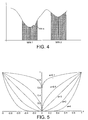
Figure 4 shows diagrammatically how a correlation curve is analysed; -
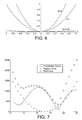
Figure 5 shows examples of the curves which might be combined with the correlation curve; -
Figure 6 is a graph which shows how the sensitivity of the curves offigure 5 to an additional factor; -
Figure 7 shows an example of a resultant curve after combination with of one of the curves offigure 5 ; -
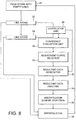
Figure 8 shows a block diagram of an embodiment of the invention. -
Figure 9 shows three different correlation curves and the topological data which is extracted from them; -
Figure 10 shows how a correlation curve can be cleansed to remove small local maxima or minima; -
Figure 11 is a flow diagram showing the procedure for detecting maxima and minima; and -
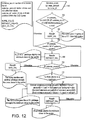
Figure 12 is a flow diagram showing the procedure for deriving a confidence measure from the information about extremes extracted by the procedure offigure 11 . - The diagram of
figure 2 is now explained with reference to the 5 pixel interpolation schemes shown infigure 1 . As mentioned above, in practice more pixels than 5 will be used and more interpolation schemes than the 3 shown infigure 1 will be used but we refer to these for ease of understanding. - In
figure 2 ,unit 1 performs the derivation of correlation data for the correlation curve shown infigure 1 . In this example 3 points are used. In practice, the number of points used will be proportional to the number of pixels used. Inunit 2, an analysis of the information contained in the correlation curve is performed to produce a confidence evaluation for the curve in the form of confidence data. This comprises a measure as to the clarity of the information contained in the correlation data. Examples of the type of correlation curve which can be generated with the correlation data are shown infigure 3 . The two left-hand side curves have clear maxima and a single minimum each. Thus, it is highly likely that the minimum value created by the SAD offigure 1 from the various sets of pairs of pixels is the correct minimum to use and therefore the correct set of pairs of pixels to use for the interpolation of the pixel of a missing line. The third curve offigure 3 has three minima and 3 maxima. Therefore the data for this graph gives no indication as to which of the minima detected is the most relevant. - The fourth example in
figure 3 gives a curve with 2 distinct minima. Either of these could be the correct one to use in determining the interpolation scheme to use. However, they are physically separated by a number of pixels and therefore it is unclear which of them should be used. - In
figure 2 , the correlation data is generated in a logical sequence, for example infigure 1 starting with the left-hand interpolation scheme and moving to the right. Whatever the scheme adopted, a logical sequence is required so that there is an incremental change in the relative positions of the pixels being used by the interpolation scheme. In graphical representation, this would mean, for example, when looking at the graph on the right-hand side offigure 1 , the first SAD point plotted is that generated by the pixels selected in the left-hand side scheme offigure 1 i.e. the diagonal line joining the pixels slope downwards to the right through the pixel to be reconstructed. For the middle point, the lines joining the pairs of pixels are vertical and forpoint 2 the lines joining the pairs of pixels slope upwards to the right. A similar type of approach is taken whatever number of pixels or whatever interpolation scheme is used. - In the confidence evaluation stage of
figure 2 , the SAD measurements fromfigure 1 are received in turn from correlation analysis inunit 1. The data as it is received is compared with previous data to determine where local minima occur. - An example of this is shown in
figure 4 for a curve which has 2 statisticallysignificant minima MIN 1 andMIN 2. There is also a minimum min x which is ignored as it's size in proportion to the rest of the curve is insignificant. Theconfidence evaluation unit 2 determines a confidence measure representing whether the correlation data is likely to produce the correct result for the interpolation scheme to be used and then uses this to select an adjustment data which is combined with the data for each point on the correlation curve. The confidence measure is supplied toadjustment curve unit 3 which selects the adjustment data to use in dependence on the output of theconfidence evaluation unit 2 and supplies the data for this curve to acombination unit 4 which combines it with a correlation data from thecorrelation curve unit 1. The resultant data is then sent to a resultantdata analysis unit 5 which can select the appropriate minimum from the resultant data and from this determine which interpolation system (seefigure 1 ) should be used in interpolating the missing pixel. - The selection of data represented by a curve which might be used by the adjustment
curve analysis unit 3 offigure 2 is shown infigure 5 . These are produced by the equation:
- In this formula b is a parameter which is adjusted in dependence on the confidence evaluation derived from the
confidence evaluation unit 2 i.e. the confidence measure, a is either a constant in the preferred embodiment or can be related to the confidence measure as well. x relates to the position of the interpolation scheme to which the confidence evaluation relates in the logical sequence of interpolation schemes. -
Figure 5 shows various different curves for different values of a with a value of b equal to 1. Although all of these could deliver good performance in specific cases, we have appreciated that the best overall curve in dealing with many situations is produced by a curve with a fixed value of a equals to 2. Because this exponential value is relatively low, the continuity of the first derivative b is more significant. Examples of this curve for various values of b are shown infigure 6 . Thus it can be seen that as b increases, the steepness of the curve increases. - The zero value of the curve is in the centre of the graph of
figure 6 andfigure 5 . This corresponds to the centre position of the logical incremental interpolation schemes. Infigure 1 this would be a central interpolation scheme with the pairs of pixels being positioned vertically with respect to the pixel to be reconstructed. - The curve selected in dependence on the confidence measure b is then passed to the resultant curve generation unit for which combines the data from the curve with the data from the
correlation curve unit 1 to produce data for a resultant curve. This is fed to a resultantcurve analysis unit 5 which looks for any minima in the resultant curve. An example of a resultant curve and the components of which it is formed is shown infigure 7 . As can be seen, a correlation curve with 2 minima which are physically separate after combination with an adjustment curve selected in accordance with a confidence measure derived from the correlation curve produces a resultant curve with one minimum much lower than the other. Thus, the position of this minimum is used to select the interpolation scheme to be used to generate the pixel. This process is performed in turn for each pixel to be interpolated on each line of each field of an input video sequence. - A more detailed block diagram of an example of a system embodying the invention is shown in
figure 8 . This comprises afield store 20 to which a field of a new video signal being converted from an interlaced video signal to a progressive scan video signal is stored. From this, each line of the field is read out in turn to linestores line store 22 and then passed toline store 24. At the same time, the next line which will be used with the first line for generating the missing lines of the field in the field store is read toline store 22. The system then analyses the lines to select the best interpolation schemes are used for each pixel in turn before passing the line stored inline store 22 toline store 24 and reading the next line of the field from thefield store 20 to theline store 22. - Once 2 lines are stored in line stores 22 and 24 a
correlation unit 26 produces, for each pixel in turn to be generated for the line position between the two lines in the line stores 22 and 24, a series of correlations in logical order for the different possible interpolation schemes to be used in generating that pixel. At the ends of the lines, not all the possible interpolations will be available. Thecorrelation unit 26 calculates for example a sum of absolute differences or a least means squared analysis of the correlation between different pairs of pixels to be used in each of the interpolation schemes. The sums of absolute differences are provided in turn for each pixel to aconfidence evaluation unit 28. When all the values from thecorrelation unit 26 have been added to the confidence evaluation unit 28 a confidence value is generated. This is related to the positions and numbers of local minima for the correlation values produced by thecorrelation unit 26. - This confidence value is then provided to an
adjustment curve selector 30 which uses it to modify a predetermined adjustment curve. In its most straightforward form the confidence value is used as a multiplier on the adjustment curve. More complex schemes can be used. Alternatively, the confidence value can be used to select between a plurality of predefined adjustment curves. - The data representing the adjustment curve is then provided from the
adjustment curve selector 30 to a resultantdata generation unit 32. Here the data from the adjustment curve is combined with the data from thecorrelation unit 26. For curves where the correlation data for a pixel which has 2 or more minima, the resultantdata generation unit 32 should by combining correlation data with the adjustment curve data produce a set of adjusted correlation data which has a clear minimum value. This clear minimum value is then detected in a resultantdata analysis unit 34. This provides data about the correlation value for a pixel which gives the minimum adjusted value. In dependence on this, aninterpolation scheme selector 36 selects an interpolation scheme to be used to generate the pixel in question. The data for that interpolation is then provided either from the line stores 22 and 24 or from thefield store 20 to aninterpolator 38 which generates the value for the missing pixel. The system then proceeds to the next of the missing pixels to be generated until all missing pixels between the lines in the 2 line stores have been generated. The system then moves the pixel data fromline store 22 toline store 24 and reads in the next available line from thefield store 20. This continues until the missing lines for the whole field have been generated and the data is available for display. - Preferably the process takes place in real time so that it can be performed on a video signal being received by a television receiver which converts the signal to a non-interlaced form ready for display.
- In an improvement on the arrangement of
figure 8 , two or more sets of the hardware offigure 8 could be provided operating in parallel in different lines of thefield store 20 to improve processing speed. - In an alternative, the system of the
figure 8 can be implemented in a dedicated processor. Two or more of these can be provided in parallel to improve the speed of processing. One possibility is to have a processor available for each of the missing lines of the field stored in thefield store 20 to minimise processing time. This of course would make the unit more expensive. - For certain pixels to be generated, the resultant
data analysis unit 34 may generate data which remains unclear. In such a situation, some form of exception processing is provided. This could involve using a different adjustment curve to improve the quality of the resultant data output. Other schemes are possible. - One further area where significant improvement in the reliability of the correct pixels being interpolated in missing lines is the confidence with which analysed correlation data can produce to a significant result. This confidence is used in the example given above to generate a confidence measure which can be used to select adjustment data to combine with the correlation data to produce a set of resultant data from which the correlation scheme most likely to produce the correct result for the pixel to be interpolated is selected. Confidence measures can be used in other methods of selecting interpolation schemes.
- We have devised a procedure for examining the correlation data to improve the reliability of the selection of interpolation schemes which can be used in combination with the adjustment data discussed above, or can be used in other methods. For example, if the confidence measure is above a predetermined value then it could be deemed to be sufficiently accurate for no adjustment to correlation data to be required and for the interpolation data to be required and for the interpolation scheme to be selected directly from the correlation data. If the confidence measure is below a predetermined value then it could be used in combination with the adjustment data discussed above or in some other scheme.
- In order to produce a confidence measure from the correlation data, the first step is to extract the topology of points from the correlation data. This is shown with regard to the graphs of
figure 9 . The top example infigure 9 shows a reasonably smooth correlation curve with a maximum close to one end and a minimum approximately two-thirds of the way along the line. The significant points of this curve are selected in the central graph to give the resultant set of the data points on the right-hand side. - A more complex graph is shown from the central line of
figure 9 . This has two distinct minima at slightly different levels with a local maximum between them. A set of data points derived from this is shown on the right-hand side. - The bottom example is the most straightforward and starts from a maximum on the left-hand side decreasing reasonably smoothly to a minimum on the right-hand side. This can be shown with only two data points.
- These data points generated now form an array of output data which comprises three elements namely:
- value of the relative extremes (relative maximum or minimum) as an integer value;
- position of the relative extremes (as an index in the correlation data); and, a flag indicating whether the extreme is a relative maximum or minimum.
- An important additional step is shown in relation to
figure 10 . This comprises what we refer to as cleaning the data. This is necessary to prevent the subsequent procedure from analysing extremes which are not significant when reconstructing the general shape or topology of the correlation data. It eliminates those maxima and minima which are too close to each other. As can be seen infigure 10 , the curve representing the correlation data has a local maximum close to the minimum value of the curve. Analysis of this by a cleaning procedure removes the local maximum leaving the two local minima and the local maximum represented by a single point in the topology. - The procedure for cleaning the correlation data is now described in relation to
figure 11 . - Initially at 40 a relative extreme is found (maximum or minimum). Then, at 42 a determination is made as to whether or not the extreme is the first point of correlation data or the last point, corresponding to the first and last interpolation schemes which could be used. If it is not, the procedure goes to step 44. If it is, then the procedure skips directly to the end and the position in the correlation curve and whether or not it is a maximum or minimum are stored in a data array. If the extreme is at some other point on the curve, then at 44, if the extreme found is a minimum and the previous extreme is a maximum, or if the extreme just found is a maximum and the previous is a minimum then the procedure passes to 46. This determines whether or not the extreme was on the left border of the correlation curve. If it was, then the amount and identity (maximum or minimum) of the new extreme are stored in a data array replacing the corresponding values of the previous extreme. If the previous extreme is not on the left border at 46 then the procedure passes to 50. If determination is made as to whether or not the present extreme is on the right-hand border, i.e. is the last extreme in the correlation curve. If it is, then the present extreme is discarded at 52. Otherwise nothing changes as at 54. If the result from 44 was that the extreme found was a minimum and the previous had not been a maximum or if the extreme found had been a maximum and the previous extreme had not been a minimum then the procedure passes to 56. A determination is made as to whether or not the extreme just found is a minimum and the previous extreme is a minimum, or if the extreme just found is a maximum and the previous is a maximum. If neither is the case then the procedure does nothing at 54. If it is the case, then the present extreme and the new extreme are averaged.
- Once the correlation data has been checked and cleaned to eliminate any extremes which are too close together, the data is passed to a processor which performs the procedure set forth in
figure 12 . The purpose of this is to examine the values of the data within the topology array and in response to this to return a value which gives an indication of the confidence of the correlation data being able to be used to select the correct interpolation scheme for reconstruction of a pixel in a missing line. This confidence measure is generated for each pixel in turn in a missing line, and for each missing line. - The example of
figure 12 uses three data values in determining the confidence measure to use. These are extreme count which is an integer value of the number of extremes but its maxima and minima found in the cleansed correlation data, extreme amount which is the magnitude of each maximum and minimum in the correlation data, and extreme ID which is a value representing the position of each maximum and minimum in the data. These values are selected from a cleansed correlation data array at 60. - At 62, a determination is made as to whether or not the extreme count value is 2 or 3 (with the first extreme being a maximum). If it is, then the curve is either a general diagonal line or a general V indicating that the minimum correlation value is relatively clear. Therefore at 64 the result is set to Sure-Val representing a high degree confidence in the correlation data. If the extreme count is not 2 or 3 then the procedure passes to 66. This determines whether the extreme count is 4 or 3 (for data where the first extreme is a minimum). If it is, then a default value Default-Val is set as a result at 68. This represents a lower degree of confidence in the ability of the correlation data to be used to select the correct interpolation scheme.
- If the extreme count is not 4 or 3 then the procedure passes to 70 which determines whether or not the extreme count is 5. If it is, then if the first extreme is determined to be a maximum at 72 then the equation shown at 74 is performed on the correlation data corresponding to the maxima and minima to derive a confidence value. If the extreme count at 70 is determined not to be 5, then it is greater than 5, a result is set to be a value called Max-Val. This indicates that there are too many maxima and minima in the correlation data and that the minima closer to the centre, i.e. the position of the pixel to be reconstructed should be emphasised.
- If at 72 the first extreme is not a maximum, then the result is set to be Default - Val as was done at 68 indicating that some emphasis should be given to the new one closer to the centre point but not so much as with max under par val.
- Using the value Sure-Val, Default-Val and Max-Val, different values to be given to the parameter b used in the selection of adjustment data as shown in
figure 6 . So, Sure-Val could correspond to a value of b 0.05, default val to a value of b of 1 and max val to a value of b of 2. Thus curves with more maxima and minima will receive more adjustment than those with fewer maxima and minima. The values can also be used in other schemes for selecting interpolations to be used when reconstructing a missing pixel. - The procedures shown in
figure 12 can be extended to look for cleansed correlation data with more maxima and minima and therefore have more values of the confidence measure to be provided. The procedure can be modified to take account of the relative size of the relative maxima or minima and their proximity in determining which one is most likely to be useful in indicating the correct interpolation scheme to use.
Claims (8)
- A method for converting an interlaced video signal to a progressive scan video signal comprising the steps of:for each pixel in each missing line of a video field in a video signal to be converted, providing correlation data for each of a set of possible interpolations between adjacent pixels to be used in reconstructing the missing pixel;deriving a confidence measure from the correlation data;determining from the confidence measure the interpolation scheme most likely to produce an accurate missing pixel; andinterpolating the missing pixel using the selected interpolation schemecharacterised in thatthe step of deriving a confidence measure comprises determining the number of maxima and minima in the correlation data and deriving the confidence measure in dependence on the number of maxima and minima so determined.
- A method according to claim 1 in which the step of determining the confidence measure including the step of determining the relative positions of the pixels from which each correlation was made and using this in deriving the confidence measure.
- A method according to claim 1 or 2 including the step of selecting adjustment data for the correlation data from the confidence measure and adjusting the correlation data with adjustment data.
- A method according to claim 3 in which the step of determining the interpolation scheme does so in dependence on the adjustment data.
- Apparatus for converting an interlaced video signal to a progressive scan video signal comprising:means for each pixel in each missing line of a video field in a video signal to be converted which provides correlation data for each set of possible interpolations between adjacent pixels to the pixel to be reconstructed;means for deriving a confidence measure from the correlation data;means for determining from the confidence measure the interpolation scheme most likely to produce an accurate missing pixel; andmeans for interpolating a missing pixel using the selected interpolation scheme;characterised in thatthe means for deriving a confidence measure comprises means for determining the number of maxima and minima in the correlation data and means for deriving the confidence measure in dependence thereon.
- Apparatus according to claim 5 in which the means for deriving a confidence measure also includes means for determining the relative positions from the pixels from which each correlation was made and means for deriving the confidence measure therefrom.
- Apparatus according to claim 5 or 6 including means for selecting adjustment data for the correlation data from the confidence measure and means for adjusting the correlation data with the adjustment data.
- Apparatus according to claim 7 in which the means for determining the interpolation scheme does so in dependence on the adjusted correlation data.
Applications Claiming Priority (2)
| Application Number | Priority Date | Filing Date | Title |
|---|---|---|---|
| GB0502598A GB2422976B (en) | 2005-02-08 | 2005-02-08 | Conversion of video data from interlaced to non-interlaced format |
| PCT/GB2006/000432 WO2006085062A2 (en) | 2005-02-08 | 2006-02-08 | Conversion of video data from interlaced to non-interlaced format |
Publications (2)
| Publication Number | Publication Date |
|---|---|
| EP1849301A2 EP1849301A2 (en) | 2007-10-31 |
| EP1849301B1 true EP1849301B1 (en) | 2016-11-16 |
Family
ID=34355979
Family Applications (1)
| Application Number | Title | Priority Date | Filing Date |
|---|---|---|---|
| EP06704581.5A Active EP1849301B1 (en) | 2005-02-08 | 2006-02-08 | Conversion of video data from interlaced to non-interlaced format |
Country Status (5)
| Country | Link |
|---|---|
| US (1) | US7518655B2 (en) |
| EP (1) | EP1849301B1 (en) |
| JP (1) | JP5209323B2 (en) |
| GB (1) | GB2422976B (en) |
| WO (1) | WO2006085062A2 (en) |
Families Citing this family (5)
| Publication number | Priority date | Publication date | Assignee | Title |
|---|---|---|---|---|
| US7587376B2 (en) * | 2005-05-26 | 2009-09-08 | International Business Machines Corporation | Reformulation of constraint satisfaction problems for stochastic search |
| GB2443858A (en) | 2006-11-14 | 2008-05-21 | Sony Uk Ltd | Alias avoiding image processing using directional pixel block correlation and predetermined pixel value criteria |
| JP5333791B2 (en) * | 2008-03-21 | 2013-11-06 | 日本電気株式会社 | Image processing method, image processing apparatus, and image processing program |
| US8355443B2 (en) * | 2008-03-27 | 2013-01-15 | CSR Technology, Inc. | Recursive motion for motion detection deinterlacer |
| GB2484071B (en) * | 2010-09-23 | 2013-06-12 | Imagination Tech Ltd | De-interlacing of video data |
Family Cites Families (11)
| Publication number | Priority date | Publication date | Assignee | Title |
|---|---|---|---|---|
| GB2277000B (en) * | 1993-04-08 | 1997-12-24 | Sony Uk Ltd | Motion compensated video signal processing |
| US5886745A (en) * | 1994-12-09 | 1999-03-23 | Matsushita Electric Industrial Co., Ltd. | Progressive scanning conversion apparatus |
| US5661525A (en) | 1995-03-27 | 1997-08-26 | Lucent Technologies Inc. | Method and apparatus for converting an interlaced video frame sequence into a progressively-scanned sequence |
| US5532751A (en) * | 1995-07-31 | 1996-07-02 | Lui; Sam | Edge-based interlaced to progressive video conversion system |
| MY117289A (en) * | 1996-01-17 | 2004-06-30 | Sharp Kk | Image data interpolating apparatus |
| JPH09200575A (en) * | 1996-01-17 | 1997-07-31 | Sharp Corp | Image data interpolation device |
| US6133957A (en) * | 1997-10-14 | 2000-10-17 | Faroudja Laboratories, Inc. | Adaptive diagonal interpolation for image resolution enhancement |
| KR100393066B1 (en) * | 2001-06-11 | 2003-07-31 | 삼성전자주식회사 | Apparatus and method for adaptive motion compensated de-interlacing video data using adaptive compensated olation and method thereof |
| JP2004072528A (en) * | 2002-08-07 | 2004-03-04 | Sharp Corp | Method and program for interpolation processing, recording medium with the same recorded thereon, image processor and image forming device provided with the same |
| GB2402288B (en) | 2003-05-01 | 2005-12-28 | Imagination Tech Ltd | De-Interlacing of video data |
| KR100580172B1 (en) * | 2003-06-27 | 2006-05-16 | 삼성전자주식회사 | De-interlacing method, apparatus, video decoder and reproducing apparatus thereof |
-
2005
- 2005-02-08 GB GB0502598A patent/GB2422976B/en active Active
- 2005-05-09 US US11/125,412 patent/US7518655B2/en active Active
-
2006
- 2006-02-08 WO PCT/GB2006/000432 patent/WO2006085062A2/en active Application Filing
- 2006-02-08 EP EP06704581.5A patent/EP1849301B1/en active Active
- 2006-02-08 JP JP2007554631A patent/JP5209323B2/en active Active
Also Published As
| Publication number | Publication date |
|---|---|
| GB2422976A (en) | 2006-08-09 |
| EP1849301A2 (en) | 2007-10-31 |
| US20060181647A1 (en) | 2006-08-17 |
| GB2422976B (en) | 2007-05-23 |
| WO2006085062A2 (en) | 2006-08-17 |
| GB0502598D0 (en) | 2005-03-16 |
| JP2008530876A (en) | 2008-08-07 |
| WO2006085062A3 (en) | 2007-01-25 |
| JP5209323B2 (en) | 2013-06-12 |
| US7518655B2 (en) | 2009-04-14 |
Similar Documents
| Publication | Publication Date | Title |
|---|---|---|
| JP4519396B2 (en) | Adaptive motion compensated frame and / or field rate conversion apparatus and method | |
| US8340186B2 (en) | Method for interpolating a previous and subsequent image of an input image sequence | |
| JP4847040B2 (en) | Ticker processing in video sequences | |
| JP3850071B2 (en) | Conversion device and conversion method | |
| KR100327395B1 (en) | Deinterlacing method based on motion-compensated inter-field interpolation | |
| JP3287864B2 (en) | Method for deriving motion vector representing motion between fields or frames of video signal and video format conversion apparatus using the same | |
| US6563550B1 (en) | Detection of progressive frames in a video field sequence | |
| TWI410895B (en) | Apparatus and methods for motion vector correction | |
| JP4932900B2 (en) | Robust super-resolution video scaling method and apparatus | |
| EP1736929A2 (en) | Motion compensation error detection | |
| EP2564588B1 (en) | Method and device for motion compensated video interpoltation | |
| EP1849301B1 (en) | Conversion of video data from interlaced to non-interlaced format | |
| EP1849300B1 (en) | Conversion of video data from interlaced to non-interlaced format | |
| JP2009207137A (en) | Method and system of processing video signal, and computer-readable storage medium | |
| KR101050135B1 (en) | Intermediate image generation method using optical information | |
| EP2619977B1 (en) | Method and apparatus for deinterlacing video data | |
| US20060176394A1 (en) | De-interlacing of video data | |
| DE112004000063B4 (en) | A method and apparatus for adaptive deinterlacing based on a phase corrected field and recording medium storing programs for performing the adaptive deinterlacing method | |
| KR100351160B1 (en) | Apparatus and method for compensating video motions | |
| JP4366836B2 (en) | Image conversion method and image conversion apparatus | |
| JP3862531B2 (en) | Image interpolation device | |
| JPH07327209A (en) | Detection of motion vector |
Legal Events
| Date | Code | Title | Description |
|---|---|---|---|
| PUAI | Public reference made under article 153(3) epc to a published international application that has entered the european phase |
Free format text: ORIGINAL CODE: 0009012 |
|
| 17P | Request for examination filed |
Effective date: 20070905 |
|
| AK | Designated contracting states |
Kind code of ref document: A2 Designated state(s): DE FR |
|
| 17Q | First examination report despatched |
Effective date: 20071213 |
|
| DAX | Request for extension of the european patent (deleted) | ||
| RBV | Designated contracting states (corrected) |
Designated state(s): DE FR |
|
| GRAP | Despatch of communication of intention to grant a patent |
Free format text: ORIGINAL CODE: EPIDOSNIGR1 |
|
| INTG | Intention to grant announced |
Effective date: 20160614 |
|
| GRAS | Grant fee paid |
Free format text: ORIGINAL CODE: EPIDOSNIGR3 |
|
| GRAA | (expected) grant |
Free format text: ORIGINAL CODE: 0009210 |
|
| AK | Designated contracting states |
Kind code of ref document: B1 Designated state(s): DE FR |
|
| REG | Reference to a national code |
Ref country code: DE Ref legal event code: R096 Ref document number: 602006050921 Country of ref document: DE |
|
| REG | Reference to a national code |
Ref country code: FR Ref legal event code: PLFP Year of fee payment: 12 |
|
| REG | Reference to a national code |
Ref country code: DE Ref legal event code: R097 Ref document number: 602006050921 Country of ref document: DE |
|
| PLBE | No opposition filed within time limit |
Free format text: ORIGINAL CODE: 0009261 |
|
| STAA | Information on the status of an ep patent application or granted ep patent |
Free format text: STATUS: NO OPPOSITION FILED WITHIN TIME LIMIT |
|
| 26N | No opposition filed |
Effective date: 20170817 |
|
| REG | Reference to a national code |
Ref country code: FR Ref legal event code: PLFP Year of fee payment: 13 |
|
| PGFP | Annual fee paid to national office [announced via postgrant information from national office to epo] |
Ref country code: FR Payment date: 20230220 Year of fee payment: 18 |
|
| PGFP | Annual fee paid to national office [announced via postgrant information from national office to epo] |
Ref country code: DE Payment date: 20230216 Year of fee payment: 18 |
|
| P01 | Opt-out of the competence of the unified patent court (upc) registered |
Effective date: 20230516 |