EP1715352A2 - Method and apparatus for diagnosing failures in a mechatronic system - Google Patents
Method and apparatus for diagnosing failures in a mechatronic system Download PDFInfo
- Publication number
- EP1715352A2 EP1715352A2 EP06006355A EP06006355A EP1715352A2 EP 1715352 A2 EP1715352 A2 EP 1715352A2 EP 06006355 A EP06006355 A EP 06006355A EP 06006355 A EP06006355 A EP 06006355A EP 1715352 A2 EP1715352 A2 EP 1715352A2
- Authority
- EP
- European Patent Office
- Prior art keywords
- model
- error
- speed
- abst
- variable
- Prior art date
- Legal status (The legal status is an assumption and is not a legal conclusion. Google has not performed a legal analysis and makes no representation as to the accuracy of the status listed.)
- Granted
Links
Images


Classifications
-
- F—MECHANICAL ENGINEERING; LIGHTING; HEATING; WEAPONS; BLASTING
- F02—COMBUSTION ENGINES; HOT-GAS OR COMBUSTION-PRODUCT ENGINE PLANTS
- F02D—CONTROLLING COMBUSTION ENGINES
- F02D41/00—Electrical control of supply of combustible mixture or its constituents
- F02D41/22—Safety or indicating devices for abnormal conditions
-
- F—MECHANICAL ENGINEERING; LIGHTING; HEATING; WEAPONS; BLASTING
- F02—COMBUSTION ENGINES; HOT-GAS OR COMBUSTION-PRODUCT ENGINE PLANTS
- F02D—CONTROLLING COMBUSTION ENGINES
- F02D41/00—Electrical control of supply of combustible mixture or its constituents
- F02D41/02—Circuit arrangements for generating control signals
- F02D41/14—Introducing closed-loop corrections
- F02D41/1401—Introducing closed-loop corrections characterised by the control or regulation method
- F02D2041/1413—Controller structures or design
- F02D2041/1415—Controller structures or design using a state feedback or a state space representation
- F02D2041/1416—Observer
-
- F—MECHANICAL ENGINEERING; LIGHTING; HEATING; WEAPONS; BLASTING
- F02—COMBUSTION ENGINES; HOT-GAS OR COMBUSTION-PRODUCT ENGINE PLANTS
- F02D—CONTROLLING COMBUSTION ENGINES
- F02D41/00—Electrical control of supply of combustible mixture or its constituents
- F02D41/02—Circuit arrangements for generating control signals
- F02D41/14—Introducing closed-loop corrections
- F02D41/1401—Introducing closed-loop corrections characterised by the control or regulation method
- F02D2041/1413—Controller structures or design
- F02D2041/143—Controller structures or design the control loop including a non-linear model or compensator
-
- F—MECHANICAL ENGINEERING; LIGHTING; HEATING; WEAPONS; BLASTING
- F02—COMBUSTION ENGINES; HOT-GAS OR COMBUSTION-PRODUCT ENGINE PLANTS
- F02D—CONTROLLING COMBUSTION ENGINES
- F02D41/00—Electrical control of supply of combustible mixture or its constituents
- F02D41/02—Circuit arrangements for generating control signals
- F02D41/14—Introducing closed-loop corrections
- F02D41/1401—Introducing closed-loop corrections characterised by the control or regulation method
- F02D2041/1433—Introducing closed-loop corrections characterised by the control or regulation method using a model or simulation of the system
- F02D2041/1434—Inverse model
-
- F—MECHANICAL ENGINEERING; LIGHTING; HEATING; WEAPONS; BLASTING
- F02—COMBUSTION ENGINES; HOT-GAS OR COMBUSTION-PRODUCT ENGINE PLANTS
- F02D—CONTROLLING COMBUSTION ENGINES
- F02D41/00—Electrical control of supply of combustible mixture or its constituents
- F02D41/02—Circuit arrangements for generating control signals
- F02D41/14—Introducing closed-loop corrections
- F02D41/1401—Introducing closed-loop corrections characterised by the control or regulation method
- F02D41/1405—Neural network control
-
- Y—GENERAL TAGGING OF NEW TECHNOLOGICAL DEVELOPMENTS; GENERAL TAGGING OF CROSS-SECTIONAL TECHNOLOGIES SPANNING OVER SEVERAL SECTIONS OF THE IPC; TECHNICAL SUBJECTS COVERED BY FORMER USPC CROSS-REFERENCE ART COLLECTIONS [XRACs] AND DIGESTS
- Y02—TECHNOLOGIES OR APPLICATIONS FOR MITIGATION OR ADAPTATION AGAINST CLIMATE CHANGE
- Y02T—CLIMATE CHANGE MITIGATION TECHNOLOGIES RELATED TO TRANSPORTATION
- Y02T10/00—Road transport of goods or passengers
- Y02T10/10—Internal combustion engine [ICE] based vehicles
- Y02T10/40—Engine management systems
Definitions
- the invention relates to a method and a device for fault diagnosis of mechatronic systems, wherein based on the analysis of existing control structures, residual signals are obtained from the control structures and an error analysis, error parameterization and error selection takes place.
- model-based fault diagnostic methods prove to be particularly suitable for use in mechatronic systems.
- the successful use of model-based fault diagnosis methods in mechatronic systems is essentially due to the fact that mechanical systems can be mathematically modeled well on the basis of the force, moment and energy balances. With the established models can, as shown in Fig. 1, the so-called Software redundancy and thus the residual signals are generated based on a comparison between the measured system sizes and their redundancy.
- An example of an error detection in the field of vehicle controls is in DE 197 50 191 A1 described.
- two measured variables are compared with one another, whereby one measured variable is converted into the other on the basis of a model and an error analysis is carried out on the basis of the difference and subsequent further measured values.
- the invention has for its object to provide a method and an apparatus for fault diagnosis, with individual errors based on the known control structure can be detected and parameterized.
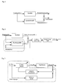
- FIG. 1 shows a typical system representation for a fault diagnosis according to the prior art with a system model (software redundancy) arranged parallel to the system, wherein a residual signal is obtained from the deviation of the output variable (actual value of the controlled variable) y and the estimated value ⁇ for this variable ,
- the block diagram outlined in FIG. 2 represents the basic structure of an observer-based fault diagnosis system.
- an observer with a system model is arranged, which determines the input quantity as well as the difference between the output variables of the real system (actual value of the controlled variable) y and the estimated value for this size ⁇ , which is based on the system model, at the entrance abut.
- the Residuentician for error diagnosis is carried out from the difference ( y - ⁇ ), wherein in subsequent steps, a Residuenausificat and a decision logic allows the determination of errors.
- the system model implemented as the core of the fault diagnosis system shown in Figure 2 in software form on a microprocessor and runs parallel to system operation.
- the setup, programming implementation and implementation of the system model require the most accurate mathematical modeling of the system as well as sufficient operating system (online / on board) computing capacity and storage space.
- the model-based residual generation is therefore often associated with high complexity due to the high complexity of mechatronic systems and high demands on computer technology and thus high costs.
- model-based controller design is a widely used method.
- system models or inverse models of the system for optimizing system behavior and for suitable adaptation (adaptive) to constantly changing environmental conditions are integrated fully or in a simplified form into control circuits and thus into mechatronic systems.
- An often used in these systems control concept is the so-called model sequence control, the structure of which is shown schematically in Figure 3.
- FIG. 3 shows the schematic representation of a model sequence control.
- the core of this control concept is that the manipulated variable u is formed based on the desired value w by an inverse model of the controlled system.
- An algorithm adapts the parameters of the inverse model on the basis of the comparison of the actual value of the controlled variable y to the estimated value of this variable, which is formed from the reference model.
- Model sequence control always contains a system model embedded in the controller structure. This structural feature makes use of the diagnostic method according to the invention. Residue signals are taken directly from the control structures embedded in a mechatronic system, without causing additional effort to form a parallel model and above all without additional online calculations.
- the fault diagnosis method is based on the embedded model following control structures, from which fault models of the residual signals are set up to parameterize and further optimally adjust the threshold values and error isolation models.
- the inventive method is based on the model sequence control structure shown in Fig. 3 and includes, by way of example, the following four different variants.
- FIG. 4 shows a variant of the model following scheme, which is often to be found in practice due to its simple structure and its low real-time computational complexity.
- the controlled system is controlled by a manipulated variable u, at whose output the actual value of the controlled variable y is measurable.
- the manipulated variable is the output variable of an inverse model of the controlled system.
- the manipulated variable u is applied to a model of the controlled system G S (s), at the output of which the difference amplified by the factor K is subtracted from the reference variable estimation and controlled variable ⁇ - y .
- This structure characterizes a classical observer structure, with the help of which a replica of the reference variable ⁇ (leading variable estimate) can be achieved.
- the control is based on a comparison between the (measured) actual value of the controlled variable y and the (online) calculation or estimation of the reference variable ⁇ from the model of the controlled system.
- the deviation of the actual value of the control variable y from the reference variable w is compensated by a correction to w via a "controller" K (s) , driven by the deviation ⁇ - y .
- a residual signal z. B. generated with the help of an observer.
- the calculation of the estimate w ⁇ ( s ) G s ( s ) u ( s ) - K ( s ) ( w ⁇ ( s ) - y ( s ) ) is basically an initial observer.
- Residual signal ⁇ ( s ) -y ( s ) or K ( s ) ( ⁇ ( s ) -y ( s )) contains the information required to detect sensor, component and actuator errors.
- y ( s ) G s ( s ) u ( s ) + ⁇ G s ( s ) u ( x ) + f s ( s ) + G K ( s ) f K ( s )
- ⁇ G s ( s ), f S ( s ), f K ( s ) are the model inaccuracies, sensor errors and component or actuator errors.
- the threshold values can be parameterized on the basis of the controller used.
- the thresholds are both in the dynamic range, z.
- Sch d w Max t
- FIG. 5 schematically illustrates the structure of an adaptive model-sequence control.
- the formation of the manipulated variable u from the desired value w is effected by an inverse model.
- the manipulated variable u further regulates the controlled system, at whose output the actual value of the controlled variable y can be measured.
- An estimate of the controlled variable ⁇ is made by an online identification of the controlled system model.
- the input of the identification is the manipulated variable u and the difference between the actual value of the controlled variable y and the estimate of the controlled variable ⁇ , with which the deviation of the model is evaluated. It can be in the Prior art known identification methods, such.
- B. Parameter estimation method or the so-called subspace methods are used.
- the controlled system model thus formed serves in a further adaptation branch for identifying the inverse model, which is used to form the manipulated variable.
- the identification of the inverse model is carried out based on the deviation of the desired value w to the branch from the model ID of the inverse model and the copy of the plant model formed estimate of the desired value w.
- ⁇ denotes the (unknown) parameter vector of the model.
- the online identification of the model parameters is performed in combination with the estimation of the output variable y .
- ⁇ ⁇ identifies the current estimate of the parameter vector.
- Residue generation is done by using the signal y - ⁇ . Since the formation of the estimate of y is based on the use of the manipulated variable u , the residual signal is generated in the context of an "open-loop" structure. Nevertheless, the residual signal is influenced indirectly by the reference variable via the identification of the inverse model.
- the inverse model used for the model-following control is modeled by means of a neural network.
- Neural networks are not only used for the modeling of technical processes, which are difficult to describe analytically, but also increasingly used in the model sequence control as a controller in the form of an inverse model.
- the use of the neural networks serves to simulate the inverse model of the controlled system and furthermore to generate the manipulated variable in such a way that the controlled variable follows the reference variable (the setpoint value) as quickly as possible.
- the training / learning of the neural network is necessary.
- the training structure / procedure shown in FIG. 7 is used in practice.
- the controlled system is modeled using a neural network.
- this NN characterized by NN 1
- u ( K - l S 1 + 1 ) ) is described with l R 1 + l S 1 inputs, the training / learning of the network is terminated when ⁇ ( k ) - y ( k ) becomes sufficiently small.
- the NN 1 is now used in the structure shown in Figure 7 as a model of the controlled system.
- u ( K ) N N 2 ( y ( K ) . y ( K - 1 ) . ⁇ . y ( K - l R 2 + 1 ) . u ( K - 1 ) . u ( K - 1 ) . ⁇ . u ( K - l S 1 + 1 ) . w ) as another NN with l R 2 + l S 1 inputs to describe the inverse model, NN 2 is trained until the difference between the output of NN 1 and the setpoint w is sufficiently small.
- control structure is used as follows. On the assumption that the NN 2 has been sufficiently trained and possible changes in the environment of the controlled system during the training, it is ensured that
- the signal y ( K ) - w ( K ) to define as residual signal. It should be noted that the residual signal y ( k ) -w ( k ) formed here, unlike the concepts described above, is generated from a closed-loop structure.
- FIG. 8 shows the fault diagnosis method according to the invention in an application to a non-linear model sequence control structure.
- a nonlinear dynamic system can be transformed under certain conditions into a linear and a nonlinear subsystem.
- the nonlinear subsystem is referred to as zero dynamics of the system.
- the task of the controller is essentially to compensate for the non-linear component with the aid of an inverse model and to excite the closed control loop by means of suitable setpoint values.
Abstract
Description
Die Erfindung betrifft ein Verfahren und eine Vorrichtung zur Fehlerdiagnose mechatronischer Systeme, wobei auf Basis der Analyse vorhandener Regelungsstrukturen Residuensignale aus den Regelungsstrukturen gewonnen werden und eine Fehleranalyse, Fehlerparametrierung und Fehlerselektion erfolgt.The invention relates to a method and a device for fault diagnosis of mechatronic systems, wherein based on the analysis of existing control structures, residual signals are obtained from the control structures and an error analysis, error parameterization and error selection takes place.
Mit der Entwicklung hin zu komplexen mechatronischen Systemen, wie z. B. Motormanagementsystemen, ESP, Robotersystemen usw. werden immer mehr leistungsfähige Sensoren, Aktuatoren und Mikroprozessoren, auf denen Regelalgorithmen implementiert werden, in diese mechatronischen Systeme eingebettet. Sie bilden in geeigneten Systemstrukturen Regelkreise, welche einzelne Komponenten und Teilsysteme so ansteuern, dass das gesamte Systemverhalten den gestellten Leistungsanforderungen entspricht. Mechatronische Systeme werden oft dort eingesetzt, wo hohe Anforderungen an Systemzuverlässigkeit und-verfügbarkeit gestellt werden. Mit dem stetig wachsenden Integrationsgrad in mechatronischen Systemen hat die Softwareredundanz gestützte Fehlerdiagnose in den vergangenen Jahren, zunächst als eine alternative Lösung zu der auf Hardwareredundanz basierenden Technologie betrachtet, stark an Bedeutung gewonnen. Die Integration softwaregestützter Fehlerdiagnosesysteme in z. B. ESP, Robotersteuerungssystemen oder in Motorsteuerungssystemen kennzeichnet eine signifikante Leistungssteigerung in der Systemzuverlässigkeit und -verfügbarkeit dieser Systeme.
Unter einer Vielzahl von Softwareredundanzgestützten Fehlerdiagnosemethoden erweisen sich die modellgestützten Methoden für den Einsatz in mechatronischen Systemen als besonders geeignet. Der erfolgreiche Einsatz modellgestützter Fehlerdiagnosemethoden in mechatronischen Systemen ist im Wesentlichen darauf zurückzuführen, dass sich mechanische Systeme anhand der Kraft-, Moment- und Energiebilanzen mathematisch gut modellieren lassen. Mit den aufgestellten Modellen kann, wie nachfolgend in Fig. 1 gezeigt, die so genannte Softwareredundanz und damit die Residuensignale anhand eines Vergleichs zwischen den gemessenen Systemgrößen und deren Redundanz generiert werden. Ein Beispiel einer Fehlerdetektion aus dem Bereich der Fahrzeugsteuerungen ist in der
Among a variety of software redundancy-based fault diagnostic methods, the model-based methods prove to be particularly suitable for use in mechatronic systems. The successful use of model-based fault diagnosis methods in mechatronic systems is essentially due to the fact that mechanical systems can be mathematically modeled well on the basis of the force, moment and energy balances. With the established models can, as shown in Fig. 1, the so-called Software redundancy and thus the residual signals are generated based on a comparison between the measured system sizes and their redundancy. An example of an error detection in the field of vehicle controls is in
Vorbekannt ist aus der
Bei beiden Verfahren erfolgt ein Abgleich von zwei Messgrößen zueinander, wobei auf Basis eines Modells eine Messgröße in die andere umgerechnet wird und auf Basis der Differenz und nachfolgender weiterer Messwerte eine Fehleranalyse erfolgt.In both methods, two measured variables are compared with one another, whereby one measured variable is converted into the other on the basis of a model and an error analysis is carried out on the basis of the difference and subsequent further measured values.
Der Erfindung liegt die Aufgabe zugrunde, ein Verfahren und eine Vorrichtung zur Fehlerdiagnose zu schaffen, wobei einzelne Fehler auf Basis der bekannten Regelungsstruktur detektierbar und parametrierbar sind.The invention has for its object to provide a method and an apparatus for fault diagnosis, with individual errors based on the known control structure can be detected and parameterized.
Diese Aufgabe wird bei gattungsgemäßen Verfahren gemäß Anspruch 1 und für gattungsgemäße Vorrichtungen gemäß Anspruch 18 erfindungsgemäß durch die jeweils kennzeichnenden Merkmale der jeweiligen Patentansprüche gelöst.This object is achieved according to the invention in the generic method according to claim 1 and for generic devices according to claim 18 by the respective characterizing features of the respective claims.
Weitere Einzelheiten der Erfindung werden in der Zeichnung anhand von schematisch dargestellten Ausführungsbeispielen beschrieben.Further details of the invention are described in the drawing with reference to schematically illustrated embodiments.
Hierbei zeigen:
- Figur 1
- eine typische Systemdarstellung mit Fehlerdiagnose gemäß dem Stand der Technik,
- Figur 2
- eine Systemdarstellung mit beobachtergestützter Fehlerdiagnose,
- Figur 3
- eine Systemdarstellung der Modellfolgeregelung,
- Figur 4
- eine Systemdarstellung der Fehlerdiagnose in einer Beobachter gestützten Modellfolgeregelungsstruktur,
- Figur 5
- Struktur einer adaptiven Modellfolgeregelung mit Residuengenerierung,
- Figur 6
- Struktur einer Modellfolgeregelung mit Neuronalem Netz,
- Figur 7
- Struktur einer Trainingsroutine für das inverse Modell,
- Figur 8
- Struktur einer nichtlinearen Modellfolgeregelung mit Fehlerdiagnose.
- FIG. 1
- a typical system representation with fault diagnosis according to the prior art,
- FIG. 2
- a system representation with observer-based fault diagnosis,
- FIG. 3
- a system representation of the model sequence control,
- FIG. 4
- a system representation of the fault diagnosis in an observer-based model sequence control structure,
- FIG. 5
- Structure of an adaptive model following scheme with residual generation,
- FIG. 6
- Structure of a model following scheme with neural network,
- FIG. 7
- Structure of a training routine for the inverse model,
- FIG. 8
- Structure of a non-linear model following scheme with fault diagnosis.
Figur 1 zeigt eine typische Systemdarstellung für eine Fehlerdiagnose nach dem Stand der Technik mit einem parallel zum System angeordneten Systemmodell (Softwareredundanz), wobei aus der Abweichung der Ausgangsgröße (Ist-Wert der Regelgröße) y und dem Schätzwert ŷ für diese Größe ein Residuensignal gewonnen wird.FIG. 1 shows a typical system representation for a fault diagnosis according to the prior art with a system model (software redundancy) arranged parallel to the system, wherein a residual signal is obtained from the deviation of the output variable (actual value of the controlled variable) y and the estimated value ŷ for this variable ,
Das in Figur 2 skizzierte Blockschaltbild stellt die Grundstruktur eines Beobachter gestützten Fehlerdiagnosesystems dar. Parallel zum System wird ein Beobachter mit einem Systemmodell angeordnet, welchem die Eingangsgröße sowie die Differenz zwischen den Ausgangsgrößen des realen Systems (Ist-Wert der Regelgröße) y und dem Schätzwert für diese Größe ŷ , die auf dem Systemmodell basiert, am Eingang anliegen. Die Residuenbildung zur Fehlerdiagnose erfolgt aus der Differenz (y - ŷ ), wobei in nachfolgenden Verfahrensschritten eine Residuenauswertung und eine Entscheidungslogik die Fehlerbestimmung ermöglicht. Es ist Stand der Technik, dass das Systemmodell als Kern des in Figur 2 dargestellten Fehlerdiagnosesystems in Softwareform auf einem Mikroprozessor implementiert wird und parallel zum Systembetrieb läuft. Die Aufstellung, programmiertechnische Umsetzung und Implementierung des Systemmodells erfordern eine möglichst genaue mathematische Modellbildung des Systems sowie im Betrieb des Systems eine ausreichende (Online/On Board) Rechenkapazität sowie Speicherplatz. Die modellgestützte Residuengenierung ist daher oft aufgrund der hohen Komplexität mechatronischer Systeme mit hohem Aufwand sowie hohem Anspruch an Rechentechnik und damit hohen Kosten verbunden.The block diagram outlined in FIG. 2 represents the basic structure of an observer-based fault diagnosis system. Parallel to the system, an observer with a system model is arranged, which determines the input quantity as well as the difference between the output variables of the real system (actual value of the controlled variable) y and the estimated value for this size ŷ , which is based on the system model, at the entrance abut. The Residuenbildung for error diagnosis is carried out from the difference ( y - ŷ ), wherein in subsequent steps, a Residuenauswertung and a decision logic allows the determination of errors. It is state of the art that the system model implemented as the core of the fault diagnosis system shown in Figure 2 in software form on a microprocessor and runs parallel to system operation. The setup, programming implementation and implementation of the system model require the most accurate mathematical modeling of the system as well as sufficient operating system (online / on board) computing capacity and storage space. The model-based residual generation is therefore often associated with high complexity due to the high complexity of mechatronic systems and high demands on computer technology and thus high costs.
Für mechatronische Systeme ist der modellgestützte Reglerentwurf ein weit verbreitetes Verfahren. Insbesondere werden in vielen Anwendungen Systemmodelle bzw. inverse Modelle des Systems zur Optimierung des Systemverhaltens und zur geeigneten Anpassung (adaptiv) an sich ständig verändernde Umgebungsbedingungen voll oder in einer vereinfachten Form in Regelkreise und damit in mechatronische Systeme integriert. Ein oft in diesen Systemen verwendetes Regelungskonzept ist die so genannte Modellfolgeregelung, deren Struktur in Figur 3 schematisch dargestellt ist.For mechatronic systems, the model-based controller design is a widely used method. In particular, in many applications, system models or inverse models of the system for optimizing system behavior and for suitable adaptation (adaptive) to constantly changing environmental conditions are integrated fully or in a simplified form into control circuits and thus into mechatronic systems. An often used in these systems control concept is the so-called model sequence control, the structure of which is shown schematically in Figure 3.
Figur 3 zeigt die schematische Darstellung einer Modellfolgeregelung. Kern dieses Regelungskonzeptes ist, dass die Stellgröße u basierend auf dem Soll-Wert w durch ein inverses Modell der Regelstrecke gebildet wird. Ein Algorithmus adaptiert dabei die Parameter des inversen Modells anhand des Vergleichs des Ist-Wertes der Regelgröße y zum Schätzwert dieser Größe, welche aus dem Referenzmodell gebildet wird. Modellfolgeregelungen enthalten dabei immer ein in die Reglerstruktur eingebettetes Streckenmodell. Dieses Strukturmerkmal macht sich das erfindungsgemäße Diagnoseverfahren zunutze. Residuensignale werden direkt aus den in einem mechatronischen System eingebetteten Regelungsstrukturen entnommen, ohne zusätzlichen Aufwand zur Bildung eines Parallelmodells und vor allem ohne zusätzliche Online-Berechnungen zu veranlassen. Das Fehlerdiagnoseverfahren basiert auf den eingebetteten Modellfolgeregelungsstrukturen, woraus Fehlermodelle der Residuensignale aufgestellt werden, um die Schwellwerte und Fehlerisolationsmodelle zu parametrisieren und ferner optimal einzustellen. Das erfindungsgemäße Verfahren geht von der in Abb. 3 dargestellten Modellfolgeregelungsstruktur aus und umfasst beispielhaft die nachfolgend dargestellten vier verschiedenen Varianten.FIG. 3 shows the schematic representation of a model sequence control. The core of this control concept is that the manipulated variable u is formed based on the desired value w by an inverse model of the controlled system. An algorithm adapts the parameters of the inverse model on the basis of the comparison of the actual value of the controlled variable y to the estimated value of this variable, which is formed from the reference model. Model sequence control always contains a system model embedded in the controller structure. This structural feature makes use of the diagnostic method according to the invention. Residue signals are taken directly from the control structures embedded in a mechatronic system, without causing additional effort to form a parallel model and above all without additional online calculations. The fault diagnosis method is based on the embedded model following control structures, from which fault models of the residual signals are set up to parameterize and further optimally adjust the threshold values and error isolation models. The inventive method is based on the model sequence control structure shown in Fig. 3 and includes, by way of example, the following four different variants.
Figur 4 zeigt eine Variante der Modellfolgeregelung, die aufgrund ihrer einfachen Struktur und ihres geringen Echtzeitrechenaufwands oft in der Praxis zu finden ist. Die Regelstrecke wird von einer Stellgröße u geregelt, wobei an deren Ausgang der Ist-Wert der Regelgröße y messbar ist. Gemäß der Modellfolgeregelstruktur ist die Stellgröße Ausgangsgröße eines inversen Modells der Regelstrecke. Von der Stellgröße u wird ein Modell der Regelstrecke GS(s) beaufschlagt, wobei an dessen Ausgang die um den Faktor K verstärkte Differenz aus Führungsgrößenschätzung und Regelgröße ŵ-y subtrahiert wird. Diese Struktur kennzeichnet eine klassische Beobachterstruktur, mit Hilfe derer eine Nachbildung der Führungsgröße ŵ (Führungsgrößenschätzung) erreicht werden kann.FIG. 4 shows a variant of the model following scheme, which is often to be found in practice due to its simple structure and its low real-time computational complexity. The controlled system is controlled by a manipulated variable u, at whose output the actual value of the controlled variable y is measurable. According to the model sequence control structure, the manipulated variable is the output variable of an inverse model of the controlled system. The manipulated variable u is applied to a model of the controlled system G S (s), at the output of which the difference amplified by the factor K is subtracted from the reference variable estimation and controlled variable ŵ - y . This structure characterizes a classical observer structure, with the help of which a replica of the reference variable ŵ (leading variable estimate) can be achieved.
Die Regelung basiert auf einem Vergleich zwischen dem (gemessenen) Ist-Wert der Regelgröße y und der (Online-)Berechnung bzw. Schätzung der Führungsgröße ŵ aus dem Modell der Regelstrecke. Die Abweichung des Ist-Wertes der Regelgröße y von der Führungsgröße w wird durch eine Korrektur an w über einen "Regler" K(s), angetrieben von der Abweichung ŵ-y, ausgeglichen.The control is based on a comparison between the (measured) actual value of the controlled variable y and the (online) calculation or estimation of the reference variable ŵ from the model of the controlled system. The deviation of the actual value of the control variable y from the reference variable w is compensated by a correction to w via a "controller" K (s) , driven by the deviation ŵ - y .
Um das Arbeitsprinzip des Reglers zu verdeutlichen, wird angenommen, dass die Regelstrecke bzw. das entsprechende inverse Modell durch Übertragungsfunktionen G S (s) bzw. ![]()
![]()
![]()
![]()
darstellen lässt. Somit gelten 


![]()
![]()
![]()
![]()
let represent. Thus apply
Bei einer geeigneten Wahl des "Reglers" K(s) kann man trotz der vorhandenen Modellungenauigkeiten (vor allem bei inversen Modellen) neben der Systemstabilität ein gutes Führungs- und Störverhalten erzielen.With a suitable choice of the "controller" K (s) can be achieved despite the existing model inaccuracies (especially in inverse models) in addition to the system stability a good management and interference behavior.
Wie bereits dargestellt wird ein Residuensignal z. B. mit Hilfe eines Beobachters generiert. Die Berechnung der Schätzung ![]()
ist im Grunde ein Ausgangsbeobachter. Somit bildet die Schätzabweichung ŵ(s)-y(s) sowie K(s)(ŵ(s)-y(s)) Residuensignale, welche sich in der Form 
darstellen lassen.As already shown, a residual signal z. B. generated with the help of an observer. The calculation of the estimate ![]()
is basically an initial observer. Y (s) and K (s) (W (s) - - y (s)) Thus, w (s) is the estimated deviation forms Residuensignale, which is in the form of
let represent.
Es ist anzumerken, dass die Stellgröße u und die Ausgangsgröße y der Sollwertschätzung 
zugeführt werden. Diese in der Literatur als "open-loop" bezeichnete Residuengenerierungsstruktur gewährleistet hohe Empfindlichkeit für die zu entdeckenden Fehler und ist von der Eigenschaft der Modellfolgeregelung unabhängig.It should be noted that the manipulated variable u and the output quantity y of the setpoint estimation
be supplied. This residuum generation structure, referred to in the literature as "open-loop," ensures high sensitivity for the errors to be detected and is independent of the model-order control property.
Das Residuensignal ŵ(s)-y(s) bzw. K(s)(ŵ(s)-y(s)) enthält die zur Entdeckung von Sensor-, Komponenten- und Aktuatorfehlern erforderlichen Informationen. Um diese Aussage zu verdeutlichen, wird angenommen, dass sich der fehlerhafte Prozess durch 
darstellen lässt, wobei mit ΔG s (s),f S (s),f K (s) die Modellungenauigkeiten, Sensorfehler und Komponenten- bzw. Aktuatorfehler bezeichnet werden. Es führt dann zu 
where ΔG s ( s ), f S ( s ), f K ( s ) are the model inaccuracies, sensor errors and component or actuator errors. It then leads to
Die obigen Gleichungen beschreiben die Dynamik der Residuensignale im Zusammenhang mit den möglichen Fehlern in Sensoren, Aktuatoren und Systemen und werden als Fehlermodell bezeichnet. Basierend auf diesen Fehlermodellen kann man die Schwellwerte anhand des verwendeten Reglers parametrisieren.The above equations describe the dynamics of the residual signals in connection with the possible errors in sensors, actuators and systems and are referred to as an error model. Based on these error models, the threshold values can be parameterized on the basis of the controller used.
Die Schwellwerte sind sowohl im dynamischen Bereich, z. B. anhand der Definitionen 
bzw. 
, wobei L -1 für die inverse Laplace-Transformierte steht,
als auch im stationären Bereich, unter der Annahme der quasi konstanten Stellgröße u, d.h. 

bzw. 
einstellbar, wobei diese Schwellwerte durch ihre Abhängigkeit von der Stellgröße sogenannte adaptive Schwellwerte bilden. Die Schwellwerte basieren also auf den Übertragungsfunktionen der Modellungenauigkeiten auf die Residuen und sind als Obergrenze des maximalen Einflusses der Störung ΔG S (Modellungenauigkeit) auf das jeweilige Residuum definiert.The thresholds are both in the dynamic range, z. For example, by definitions
respectively.
where L -1 stands for the inverse Laplace transform,
as well as in the stationary area, assuming the quasi-constant manipulated variable u, ie
respectively.
adjustable, these thresholds form by their dependence on the manipulated variable so-called adaptive thresholds. The threshold values are thus based on the transfer functions of the model inaccuracies on the residuals and are defined as the upper limit of the maximum influence of the disturbance Δ G S (model inaccuracy) on the respective residual.
Die möglichen Fehler sind weiterhin durch den Einsatz von Nachfiltern, z. B. durch die Nachfilter mit den Übertragungsfunktionen R 1(s), R 2(s) im Falle des Residuums ŵ(s)-y(s),
wobei R 1(s) so zu wählen ist, dass 

![]()
bzw. R 2(s) so zu wählen ist, dass 

![]()
where R 1 ( s ) is to be chosen such that
![]()
or R 2 ( s ) is to be chosen so that ![]()
Weiterhin kann der aufgetretene und lokalisierte Fehler identifiziert, d. h. seine Größe über die Zusammenhänge 
abgeschätzt werden. Mit f̂ S bzw. f̂ K liegt dann zusätzlich eine Fehlergrößenschätzung für den Sensor- bzw. Aktuator- bzw. Komponentenfehler vor. Gleiches Vorgehen führt zu zwei weiteren Nachfiltern und vergleichbaren Ergebnissen im Falle der Betrachtung des Residuums K(s)(ŵ(s)-y(s)).Furthermore, the occurred and localized error can be identified, ie its size via the relationships
be estimated. With f S or f K is then also an error size estimate for the sensor or actuator or component error before. The same procedure leads to two further postfilters and comparable results in the case of consideration of the residual K ( s ) ( ŵ ( s ) - y ( s )).
In Figur 5 ist die Struktur einer adaptiven Modellfolgeregelung schematisch dargestellt.
Entsprechend dem Grundprinzip der Modellfolgeregelung erfolgt die Bildung der Stellgröße u aus dem Soll-Wert w durch ein inverses Modell. Die Stellgröße u regelt weiterhin die Regelstrecke, an deren Ausgang der Ist-Wert der Regelgröße y messbar ist. Es erfolgt eine Schätzung der Regelgröße ŷ durch eine Online-Identifikation des Regelstreckenmodells. Eingang der Identifikation ist die Stellgröße u sowie die Differenz vom Ist-Wert der Regelgröße y und Schätzung der Regelgröße ŷ, mit welcher die Abweichung des Modells bewertet wird. Es können dabei im Stand der Technik bekannte Identifikationsverfahren, wie z. B. Parameterschätzverfahren oder die so genannten Subspace-Verfahren verwendet werden. Das so gebildete Regelstreckenmodell dient in einem weiteren Adaptionszweig zur Identifikation des inversen Modells, welches zur Bildung der Stellgröße genutzt wird. Die Identifikation des inversen Modells erfolgt dabei anhand der Abweichung des Soll-Wertes w zu dem aus dem Modellzweig Identifikation des inversen Modells und der Kopie des Regelstreckenmodells gebildeten Schätzung des Soll-Wertes ŵ.FIG. 5 schematically illustrates the structure of an adaptive model-sequence control.
In accordance with the basic principle of the model sequence control, the formation of the manipulated variable u from the desired value w is effected by an inverse model. The manipulated variable u further regulates the controlled system, at whose output the actual value of the controlled variable y can be measured. An estimate of the controlled variable ŷ is made by an online identification of the controlled system model. The input of the identification is the manipulated variable u and the difference between the actual value of the controlled variable y and the estimate of the controlled variable ŷ , with which the deviation of the model is evaluated. It can be in the Prior art known identification methods, such. B. Parameter estimation method or the so-called subspace methods are used. The controlled system model thus formed serves in a further adaptation branch for identifying the inverse model, which is used to form the manipulated variable. The identification of the inverse model is carried out based on the deviation of the desired value w to the branch from the model ID of the inverse model and the copy of the plant model formed estimate of the desired value w.
Um das Regelungskonzept zu verdeutlichen, wird die Regelstrecke durch ![]()
modelliert, wobei θ den (unbekannten) Parametervektor des Modells bezeichnet. Die Online-Identifikation der Modellparameter wird kombiniert mit der Schätzung der Ausgangsgröße y durchgeführt. Dieser Vorgang lässt sich schematisch durch 
beschreiben, wobei Ψ(u,y-ŷ) eine Abbildung, also einen allgemeinen (mathematischen) Zusammenhang zwischen Stellgröße, Regelgröße und Systemparametern beschreibt. Dieser könnte beispielsweise eine klassische lineare oder nichtlineare Beobachterstruktur sein.
![]()

![]()
where θ denotes the (unknown) parameter vector of the model. The online identification of the model parameters is performed in combination with the estimation of the output variable y . This process can be done schematically
describe where Ψ ( u , y - ŷ ) describes a mapping, ie a general (mathematical) relationship between control value, controlled variable and system parameters. For example, this could be a classical linear or nonlinear observer structure.
![]()
Mit einer Identifikation der Modellparameter kann man dann davon ausgehen, dass 
und somit das Ziel der Modellfolgeregelung 
erreicht wird.With an identification of the model parameters one can assume that
and thus the goal of the model following scheme
is reached.
Die Residuengenerierung erfolgt durch die Nutzung des Signals y-ŷ. Da die Bildung der Schätzung von y auf der Nutzung der Stellgröße u basiert, wird das Residuensignal im Kontext einer "open-loop"-Struktur generiert. Dennoch wird das Residuensignal indirekt durch die Führungsgröße über die Identifikation des inversen Modells beeinflusst.Residue generation is done by using the signal y - ŷ . Since the formation of the estimate of y is based on the use of the manipulated variable u , the residual signal is generated in the context of an "open-loop" structure. Nevertheless, the residual signal is influenced indirectly by the reference variable via the identification of the inverse model.
Wird nun angenommen, dass 
ist, so gilt 
wodurch die Dynamik des zuvor definierten Residuums beschrieben wird und die sogenannten Fehlermodelle definiert sind. Der Schwellwert ist sowohl im dynamischen Bereich, z. B. anhand der Definitionen 
, wobei L -1 für die inverse Laplace-Transformierte steht, als auch im stationären Bereich, unter der Annahme der quasi konstanten Stellgröße u, d. h. 

einstellbar und kennzeichnet den maximalen Einfluss der Störung (Modellungenauigkeit) auf das Residuumsignal. Der Schwellwert wird durch seine Abhängigkeit von den Parameterungenauigkeiten auch als adaptiver Schwellwert bezeichnet.Now it is assumed that
is, then applies
whereby the dynamics of the previously defined residual is described and the so-called error models are defined. The threshold is both in the dynamic range, z. For example, by definitions
, where L -1 stands for the inverse Laplace transform, as well as in the stationary region, assuming the quasi-constant manipulated variable u, ie
adjustable and indicates the maximum influence of the disturbance (model inaccuracy) on the residual signal. The threshold is also referred to as an adaptive threshold due to its dependency on the parameter inaccuracies.
Die möglichen Fehler sind weiterhin durch den Einsatz von Nachfiltern, z. B. durch die Nachfilter mit den Übertragungsfunktionen R 1(s), R 2(s),
wobei R 1(s) so zu wählen ist, dass R 1(s)G K (s) << R 1(s)f S (s) und damit
R 1(s)(y(s)-ỹ(s)) ≈ R 1(s)[ΔG s (s,α,β,γ)u(s)+f s (s)] gilt, wodurch über den Zusammenhang |R 1(s)(y(s)-ŷ(s))|> Sch dy auf einen Fehler f s (s) geschlossen werden kann,
bzw. R 2(s) so zu wählen ist, dass R 2(s)f s (s)<<R 2(s)G K (s) und damit R 2(s)(y(s)-ŷ(s)) ≈ R 2(s)[ΔG s (s,α,β,γ)u(s) + G K (s)f K (s)] gilt, wodurch über den Zusammenhang |R 2(s)(y(s)-ŷ(s))|>Sch dy auf einen Fehler f K (s) geschlossen werden kann und damit eine Lokalisierung, d. h. eine Bestimmung der Fehlerquelle, sichergestellt ist.The possible errors are still through the use of post filters, z. B. by the postfilter with the transfer functions R 1 ( s ), R 2 ( s ),
where R 1 ( s ) is to be chosen such that R 1 ( s ) G K ( s ) << R 1 ( s ) f S ( s ) and thus
R 1 ( s ) ( y ( s ) - ỹ ( s )) ≈ R 1 ( s ) [Δ G s ( s , α, β, γ) u ( s ) + f s ( s )] the context | R 1 ( s ) ( y ( s ) - ŷ ( s )) |> Sch dy can be closed to an error f s ( s ),
or R 2 ( s ) is to be chosen such that R 2 ( s ) f s ( s ) << R 2 ( s ) G K ( s ) and thus R 2 ( s ) ( y ( s ) - ŷ ( s )) ≈ R 2 ( s ) [Δ G s ( s , α, β, γ) u ( s ) + G K ( s ) f K ( s )], whereby the relation | R 2 ( s ) ( y ( s ) - ŷ ( s )) |> Sch dy on an error f K ( s ) can be closed and thus a localization, ie a determination of the error source is ensured.
Weiterhin kann der aufgetretene und lokalisierte Fehler identifiziert, d. h. seine Größe über die Zusammenhänge ![]()
![]()
![]()
![]()
In einer weiteren Ausführungsform gemäß Figur 6 wird das für die Modellfolgeregelung genutzte inverse Modell mittels eines Neuronalen Netzes modelliert. Neuronale Netze (NN) werden nicht nur zur Modellierung technischer Prozesse, welche analytisch schwer zu beschreiben sind, sondern auch zunehmend in der Modellfolgeregelung als Regler in Form eines inversen Modells verwendet. Wie in Figur 6 beschrieben dient der Einsatz der Neuronalen Netze dazu, das inverse Modell der Regelstrecke nachzubilden und ferner die Stellgröße so zu generieren, dass die Regelgröße der Führungsgröße (dem Soll-Wert) schnellstmöglich folgt.In a further embodiment according to FIG. 6, the inverse model used for the model-following control is modeled by means of a neural network. Neural networks (NN) are not only used for the modeling of technical processes, which are difficult to describe analytically, but also increasingly used in the model sequence control as a controller in the form of an inverse model. As described in FIG. 6, the use of the neural networks serves to simulate the inverse model of the controlled system and furthermore to generate the manipulated variable in such a way that the controlled variable follows the reference variable (the setpoint value) as quickly as possible.
Für eine erfolgreiche Modellierung des Neuronalen Netzes d. h. für die Bildung des inversen Modells für die Modellfolgeregelung mittels eines Neuronalen Netzes ist das Training/Lernen des Neuronalen Netzes notwendig. Zu diesem Zweck wird in der Praxis die in Figur 7 gezeigte Trainingsstruktur/-prozedur verwendet. Zunächst wird die Regelstrecke mit Hilfe eines Neuronalen Netzes nachgebildet. Sei angenommen, dass dieses NN, gekennzeichnet durch NN1, durch 
mit l R1 + l S1 Eingängen beschrieben wird, wird das Training/Lernen des Netzes dann beendet, wenn ŷ(k)-y(k) ausreichend klein wird. Das NN1 wird nun in die in Figur 7 dargestellte Struktur als Modell der Regelstrecke eingesetzt. Mit 
als weiteres NN mit l R2+l S1 Eingängen zur Beschreibung des inversen Modells, wird NN2 so lange trainiert, bis die Differenz zwischen der Ausgangsgröße des NN1 und dem Soll-Wert w ausreichend klein ist.For a successful modeling of the neural network, ie for the formation of the inverse model for the model following regulation by means of a neural network, the training / learning of the neural network is necessary. For this purpose, the training structure / procedure shown in FIG. 7 is used in practice. First, the controlled system is modeled using a neural network. Suppose that this NN, characterized by NN 1 , is through
is described with l R 1 + l S 1 inputs, the training / learning of the network is terminated when ŷ ( k ) - y ( k ) becomes sufficiently small. The NN 1 is now used in the structure shown in Figure 7 as a model of the controlled system. With
as another NN with l R 2 + l S 1 inputs to describe the inverse model, NN 2 is trained until the difference between the output of NN 1 and the setpoint w is sufficiently small.
Für die Anwendung zur Fehlerdiagnose wird die Regelungsstruktur wie folgt genutzt. Unter der Voraussetzung, dass das NN2 ausreichend und mögliche Veränderungen in der Umgebung der Regelstrecke während des Trainings mit berücksichtigt trainiert wurde, wird gewährleistet, dass 
Es liegt somit nahe, das Signal 
als Residuensignal zu definieren. Es ist anzumerken, dass das hier gebildete Residuensignal y(k)-w(k) im Gegensatz zu den oben beschriebenen Konzepten aus einer "closed-loop"-Struktur generiert wird.It is therefore obvious, the signal
to define as residual signal. It should be noted that the residual signal y ( k ) -w ( k ) formed here, unlike the concepts described above, is generated from a closed-loop structure.
Um den Einfluss der möglichen Fehler auf das Residuensignal zu verdeutlichen, wird der Einfachheit halber angenommen, dass sich Sensor- und Aktuatorfehler durch 
modellieren lassen und ferner im fehlerfreien Fall 
gilt. f(●) kennzeichnet eine nichtlineare Funktion, die die Regelstrecke beschreibt und sich durch das NN1 ausreichend gut nachbilden lässt. Es gilt dann im Allgemeinen 
![]()
modeled and also in error-free case
applies. f (●) denotes a non-linear function that describes the controlled system and that can be mapped sufficiently well by NN 1 . It then applies in general ![]()
Als ein Beispiel kann man die Wirkung eines Sensorfehlers aus der obigen Darstellung durch 
![]()

beschreiben. Basierend auf diesem Fehlermodell kann man dann den Schwellwert parametrisieren, einstellen und die möglichen Fehler lokalisieren und unter gewissen Bedingungen identifizieren.As an example, one can see the effect of a sensor error from the above illustration ![]()
describe. Based on this error model, one can then parameterize the threshold value, set it and locate the possible errors and identify them under certain conditions.
Figur 8 zeigt das erfindungsgemäße Fehlerdiagnoseverfahren in einer Anwendung auf eine nichtlineare Modellfolgeregelstruktur.FIG. 8 shows the fault diagnosis method according to the invention in an application to a non-linear model sequence control structure.
Basierend auf dem Konzept der Systemlinearisierung durch (Zustands-) Rückkopplung wird das Schema der Modellfolgeregelung erfolgreich zur Regelung nichtlinearer Systeme eingesetzt. Vor allem im Bereich der Regelung mechatronischer Systeme wird damit der Stand der Technik markiert. Zur Erläuterung des Arbeitsprinzips der Regler wird das in Abb. 7 vereinfacht dargestellte Modellfolgeregelungssystem herangezogen.Based on the concept of system linearization through (state) feedback, the model-tracking scheme is successfully used to control nonlinear systems. Especially in the field of control of mechatronic systems thus the state of the art is marked. To explain the principle of operation of the controller, the model following control system shown in simplified form in Fig. 7 is used.
Es wird angenommen, dass sich die Regelstrecke durch 
mit y Abst ,y Geschw als Messungen des Abstands und der Geschwindigkeit darstellen lässt. Eine Modellfolgeregelung erfolgt dann durch die Einstellung des Reglers der Form 
wobei ![]()

with y Abst , y Display speed as measurements of the distance and the speed. A model sequence control then takes place by setting the controller of the form
in which ![]()
Damit ist ersichtlich, dass sich durch eine geeignete Einstellung der beiden Parameter 
zwei Residuensignale bilden.This shows that this can be achieved by a suitable setting of the two parameters
form two residual signals.
Im Allgemeinen lässt sich ein nichtlineares, dynamisches System unter bestimmten Bedingungen in ein lineares und ein nichtlineares Teilsystem transformieren. Das nichtlineare Teilsystem wird als Zero-Dynamik des Systems bezeichnet. Die Aufgabe des Reglers besteht nun im Wesentlichen darin, mit Hilfe eines inversen Modells den nichtlinearen Anteil zu kompensieren und den geschlossenen Regelkreis durch geeignete Soll-Werte zu erregen.In general, a nonlinear dynamic system can be transformed under certain conditions into a linear and a nonlinear subsystem. The nonlinear subsystem is referred to as zero dynamics of the system. The task of the controller is essentially to compensate for the non-linear component with the aid of an inverse model and to excite the closed control loop by means of suitable setpoint values.
Es werden die möglichen Sensor- und Aktuatorfehler durch 
modelliert. Es gilt dann 
, woraus man den Einfluss der einzelnen Fehler berechnen und somit die Grundlage für eine Residuenauswertung zwecks Fehlerdetektion und -lokalisierung schaffen kann.It will the possible sensor and actuator errors through
modeled. It then applies
from which one can calculate the influence of the individual errors and thus create the basis for a Residuenauswertung for the purpose of error detection and localization.
Es ist anzumerken, dass die hier beschriebene Residuengenerierung in einer "closed-loop"-Struktur realisiert wird.It should be noted that the residue generation described here is realized in a closed-loop structure.
w Führungsgröße (Soll-Wert)
ŵ Schätzwert der Führungsgröße
y Regelgröße (Ist-Wert)
ŷ Schätzwert der Regelgröße
u Stellgröße
GS(s) Streckenmodell
GS -1(s) inverses Streckenmodell
K Übergangsfunktion Regler für Soll-Wertkorrektur
GK Fehlerübertragungsfunktion der Aktuator- oder Komponentenfehler (bezogen auf Regelgröße)
fS(s) Sensorfehler
fK(s) Aktuator- oder Komponentenfehler
f̂ S Fehlergrößenschätzung Sensorfehler
f̂ K Fehlergrößenschätzung Aktuator- oder Komponentenfehler
ϑ Parametervektor des Modells
Ψ Abbildung (allg. math.)
![]()
IS1 Anzahl gespeicherter Abtastschritte der Stellgröße (NN1 & NN2)
IR1 Anzahl gespeicherter Abtastschritte der Regelgröße (NN1)
IR2 Anzahl gespeicherter Abtastschritte der Regelgröße (NN2)
NN Neuronales Netz (Abk.)
SCHdw Schwellwert aus Abschätzung Störeinfluss auf Residuum
SCHds Schwellwert aus Abschätzung Störeinfluss auf Residuum
SCHdy Schwellwert aus Abschätzung Störeinfluss auf Residuumw Command value (target value)
ŵ estimated value of the reference variable
y controlled variable (actual value)
ŷ estimated value of the controlled variable
u manipulated variable
G S (s) route model
G S -1 (s) inverse route model
K Transition function controller for setpoint correction
G K Error transfer function of the actuator or component error (relative to controlled variable)
f S (s) sensor error
f K (s) Actuator or component error
f S Error size estimation Sensor error
f K Error size estimation actuator or component error
θ parameter vector of the model
Ψ Figure (general math.)
![]()
I S1 number of stored sampling steps of the manipulated variable (NN1 & NN2)
I R1 number of stored sampling steps of the controlled variable (NN1)
I R2 number of stored sampling steps of the controlled variable (NN2)
NN neural network (abbr.)
SCH dw Threshold from estimation Interference on residual
SCH ds Threshold from estimation disturbance on residual
SCH dy Threshold from estimation Disturbance on residual
Claims (20)
dadurch gekennzeichnet,
dass zur Fehlerdiagnose die in das Regelungssystem eingebettete Modellfolgeregelung betrachtet wird und die Fehlerdiagnose auf Basis wenigstens eines Schätzwertes, der aus dem in der Modellfolgeregelung enthaltenen Modell der Regelstrecke abgeleitet wird, erfolgt.Method for error diagnosis of a regulated mechatronic system whose control structures have at least one model following scheme,
characterized,
in that for fault diagnosis the model following scheme embedded in the control system is considered and the fault diagnosis is based on at least one estimated value derived from the model of the controlled system contained in the model following scheme.
dadurch gekennzeichnet,
dass zur Fehlerdiagnose die Differenz einer Schätzung der Führungsgröße (ŵ), die aus dem in der Modellfolgeregelung enthaltenen Modell der Regelstrecke abgeleitet wird, und des Ist-Wertes der Regelgröße (y) erfolgt.Method according to claim 1,
characterized,
in that the difference between an estimate of the reference variable ( ŵ ) derived from the model of the controlled system contained in the model sequence control and the actual value of the controlled variable (y) takes place for error diagnosis.
dadurch gekennzeichnet,
dass zur Fehlerdiagnose die Differenz ŵ-y gebildet wird, wobei sich ŵ aus

characterized,
that the difference ŵ - y is formed for error diagnosis, where ŵ is off
dadurch gekennzeichnet,
dass der Schwellwert zur Abschätzung der Störeinflüsse auf das jeweilige Residuum und damit zur Vermeidung von Fehlalarmen im Rahmen der Fehlererkennung in Abhängigkeit von den Reglerparametern gebildet wird.Method according to claim 3,
characterized,
is that the threshold value for estimating the interference on the respective residue and thus to avoid false alarms in the context of fault detection formed as a function of the controller parameters.
dadurch gekennzeichnet,
dass der Schwellwert zur Abschätzung der Störeinflüsse auf das jeweilige Residuum und damit zur Vermeidung von Fehlalarmen im Rahmen der Fehlererkennung in Abhängigkeit von den Reglerparametern mit

wobei L -1 für die inverse Laplace-Transformierte steht, oder im stationären Bereich unter der Annahme der quasi konstanten Stellgröße anhand von

gebildet wird.Method according to claim 4,
characterized,
that the threshold value for the estimation of the disturbing influences on the respective residuum and thus for the avoidance of false alarms within the scope of the error detection as a function of the controller parameters
where L -1 stands for the inverse Laplace transform, or in the stationary range, assuming the quasi-constant manipulated variable based on
is formed.
dadurch gekennzeichnet,
dass der Fehler durch den Einsatz von Nachfiltern lokalisiert wird.Method according to one of the preceding claims,
characterized,
that the error is localized by the use of post filters.
dadurch gekennzeichnet,
dass der Fehler durch den Einsatz von Nachfiltern vorzugsweise mittels

bzw.

für das Residuum ŵ(s) - y(s) (durch entsprechend gleiches Vorgehen auch
für das Residuum K(S)(ŵ(s) - y(s)) zu definieren) lokalisiert wird.Method according to one of the preceding claims,
characterized,
that the error through the use of post-filters preferably by means of
respectively.
for the residual ŵ ( s ) - y ( s ) (by following the same procedure also
will define localized) - for residual K (S) (y (s) w (s)).
dadurch gekennzeichnet,
dass eine Fehlerschätzung anhand von

characterized,
that an error estimate based on
dadurch gekennzeichnet,
dass zur Fehlerdiagnose die Differenz einer Schätzung der Regelgröße ŷ, die aus dem in der Modellfolgeregelung enthaltenen Modell der Regelstrecke abgeleitet wird, und des Ist-Wertes der Regelgröße (y) erfolgt.Method according to claim 1,
characterized,
that the error diagnosis is the difference of an estimate of the controlled variable ŷ , which is derived from the model of the controlled system contained in the model sequence control, and the actual value of the controlled variable (y).
dadurch gekennzeichnet,
dass der Schätzwert der Regelgröße aus der Differenz des Ist-Wertes der Regelgröße y und des Schätzwertes der Regelgröße ŷ erfolgt, wobei ein zur Regelung in der Modellfolgeregelung benutztes, inverses Modell auf Basis der Identifikation des Regelstreckenmodells über den Abgleich des Soll-Wertes w zur Schätzgröße des Soll-Wertes ŵ adaptiert wird und die Stellgröße u des Modellfolgereglers aus dem so adaptierten, inversen Modell gebildet wird.Method according to claims 9 and 1,
characterized,
that the estimated value of the controlled variable from the difference of the actual value y of the controlled variable and is carried out of the estimated value of the controlled variable y, wherein a regulating in the model follower control-used, inverse model based on the identification of the controlled system model through the adjustment of the desired value w to the estimated value the setpoint value ŵ is adapted and the manipulated variable u of the model sequence controller is formed from the thus adapted, inverse model.
dadurch gekennzeichnet,
dass die Regelstrecke mit y(s)=G S (s,θ)u(s) modelliert wird, wobei θ der Parametervektor des Modells ist und die Online-Identifikation der Modellparameter kombiniert mit der Schätzung der Ausgangsgröße y durchgeführt wird, wobei gilt

und Ψ(u,y-ŷ) eine Abbildung und θ̂ die aktuelle Schätzung des Parametervektors ist, weiterhin die Adaption des Parametervektors ϑ des inversen Modells durch


und somit das Ziel der Modellfolgeregelung

erreicht wird, wobei die Residuen durch die Nutzung des Signals y - ŷ gebildet werden und sich für y(s) = G s (s,θ)u(s)+f s (s)+ G K (s)f K (s) die Residuen zu

characterized,
in that the controlled system is modeled with y ( s ) = G s ( s, θ ) u ( s ), where θ is the parameter vector of the model and the online identification of the model parameters combined with the estimation of the output variable y is performed
and Ψ ( u , y - ŷ ) is an image and θ is the current estimate of the parameter vector, further the adaptation of the parameter vector θ of the inverse model
and thus the goal of the model following scheme
whereby the residuals are formed by the use of the signal y - ŷ and for y ( s ) = G s ( s , θ) u ( s ) + f s ( s ) + G K ( s ) f K ( s ) the residuals too
dadurch gekennzeichnet,
dass der Schwellwert anhand der Definition Sch dy = max t |ΔG s (s,α,β,γ)u(s)| ,
wobei L -1 für die inverse Laplace-Transformierte steht, eingestellt wird.Method according to claim 11,
characterized,
that the threshold value based on the definition Sch dy = max t | Δ G s (s, α, β, γ) u (s) | .
where L -1 stands for the inverse Laplace transform.
dadurch gekennzeichnet,
dass der Fehler durch den Einsatz von Nachfiltern lokalisiert wird, wobei vorzugsweise die Übertragungsfunktionen R1(s) und R2(s) beispielhaft für das Residuum ŵ(s) - y(s) so zu wählen sind, dass


und/oder R 2(s) so zu wählen ist, dass


characterized,
that the error is localized by the use of postfilters, wherein preferably the transfer functions R 1 (s) and R 2 (s) are to be selected by way of example for the residue ŵ ( s ) -y ( s ) such that
and / or R 2 ( s ) is to be chosen such that
dadurch gekennzeichnet,
dass eine Größenschätzung des Fehlers mit

erfolgt.Method according to claim 11,
characterized,
that a size estimate of the error with
he follows.
dadurch gekennzeichnet,
dass zur Fehlerdiagnose ein mittels eines Neuronalen Netzes gebildetes, inverses Modell für die Modellfolgeregelung verwendet wird, wobei das inverse Modell in einem zweistufigen Verfahren generiert wird, indem ein Neuronales Netz NN1 für die Regelstrecke auf Basis der Abweichung einer Schätzung der Regelgröße ŷ und des Ist-Wertes der Regelgröße (y) erfolgt, wobei das so trainierte Neuronale Netz NN1 als Modell der Regelstrecke für das Training des Neuronalen Netzes NN2, welches für die Modellfolgeregelung verwendet wird, genutzt wird, wobei das Neuronale Netz NN2 anhand der Abweichung des Soll-Wertes zur Schätzung der Regelgröße ŷ aus dem Modell der Regelstrecke trainiert wird und die Residuen zur Fehlerauswertung aus der Abweichung des Soll-Wertes w zum Ist-Wert der Regelgröße y gebildet werden.Method according to claim 1,
characterized,
is that used to diagnose an image formed by means of a neural network, inverse model for the model follower control, the inverse model is generated in a two step process by a neural network NN1 ŷ an estimation of the control variable for the controlled system on the basis of the deviation and of the actual The value of the controlled variable (y) takes place, whereby the neural network NN1 thus trained is used as a model of the controlled system for the training of the neural network NN2, which is used for the model following control, wherein the neural network NN2 is based on the deviation of the desired value from Estimation of the controlled variable ŷ is trained from the model of the controlled system and the residuals for error evaluation from the deviation of the desired value w to the actual value of the controlled variable y are formed.
dadurch gekennzeichnet,
dass das für die Modellfolgeregelung mittels des Neuronalen Netzes gebildete inverse Streckenmodell adaptiv modifizierbar ist und die Regelabweichung als Residualsignal genutzt wird, wobei ein Modell für die Sensorfehler gemäß


gebildet wird und auf Grund des Fehlermodells die Sensorfehler lokalisiert und identifiziert werden

characterized,
in that the inverse path model formed for the model following control by means of the neural network is adaptively modifiable and the control deviation is used as a residual signal, wherein a model for the sensor errors according to
is formed and based on the error model, the sensor errors are located and identified
dadurch gekennzeichnet,
dass zur Fehlerdiagnose die in das Regelungssystem eingebettete Modellfolgeregelung genutzt wird, wobei diese eine adaptive Modellfolgeregelung ist, bei welcher eine Systemzerlegung in ein lineares Teilsystem und ein nichtlineares Teilsystem erfolgt und die Kompensation der nichtlinearen Dynamik anhand des inversen Modells des nichtlinearen Teilsystems erfolgt wobei ein resultierender linearer Anteil verbleibt und die Differenz zwischen der Führungsgröße und der Regelgröße zur Bildung der Fehlermodelle genutzt wird.Method according to claim 1,
characterized,
in that for error diagnosis the model following scheme embedded in the control system is used, which is an adaptive model following scheme in which a system decomposition into a linear subsystem and a nonlinear subsystem takes place and the compensation of the nonlinear dynamics is done using the inverse model of the nonlinear subsystem wherein a resulting linear The proportion remains and the difference between the reference variable and the controlled variable is used to form the error models.
dadurch gekennzeichnet,
dass aus der Führungsgröße und der Regelgröße ein Residuensignal gebildet wird, welches aufgrund der Eigenschaften der nichtlinearen adaptiven Modellfolgeregelung Strecken- und Aktuatorfehler beschreibt und ein Fehlermodell wie folgt beschrieben wird:

wobei basierend auf dem obigen Modell Fehler detektiert und lokalisiert werden.Method according to claim 17,
characterized,
that a residual signal is formed from the reference variable and the controlled variable, which describes path and actuator errors on the basis of the properties of the nonlinear adaptive model-sequence control and an error model is described as follows:
wherein errors are detected and located based on the above model.
dadurch gekennzeichnet,
dass es zur Durchführung des Verfahrens nach Anspruch 1 - 16 geeignet ist, wenn es auf einem Computer ausgeführt wird, wobei es auf einem Speicher des Computers abgelegt ist.Computer program
characterized,
that it is suitable for carrying out the method according to claim 1-16 when it is executed on a computer, wherein it is stored on a memory of the computer.
dadurch gekennzeichnet,
dass diese einen Speicher umfasst, auf welchem ein Computerprogramm nach Anspruch 19 abgelegt ist.Control and regulating device for operating an internal combustion engine,
characterized,
that it comprises a memory on which a computer program according to claim 19 is stored.
Applications Claiming Priority (1)
| Application Number | Priority Date | Filing Date | Title |
|---|---|---|---|
| DE200510018980 DE102005018980B4 (en) | 2005-04-21 | 2005-04-21 | Method and device for fault diagnosis of mechatronic systems |
Publications (3)
| Publication Number | Publication Date |
|---|---|
| EP1715352A2 true EP1715352A2 (en) | 2006-10-25 |
| EP1715352A3 EP1715352A3 (en) | 2012-04-18 |
| EP1715352B1 EP1715352B1 (en) | 2019-04-24 |
Family
ID=36686111
Family Applications (1)
| Application Number | Title | Priority Date | Filing Date |
|---|---|---|---|
| EP06006355.9A Active EP1715352B1 (en) | 2005-04-21 | 2006-03-28 | Method and apparatus for diagnosing failures in a mechatronic system |
Country Status (2)
| Country | Link |
|---|---|
| EP (1) | EP1715352B1 (en) |
| DE (1) | DE102005018980B4 (en) |
Cited By (7)
| Publication number | Priority date | Publication date | Assignee | Title |
|---|---|---|---|---|
| FR2923545A1 (en) * | 2007-11-12 | 2009-05-15 | Peugeot Citroen Automobiles Sa | Supercharged engine assembly diagnosing method for engine i.e. internal combustion engine, of automobile, involves comparing equivalence between real states and measurements with equivalence between states and measurements without failure |
| DE102008015909B3 (en) * | 2008-03-27 | 2009-12-03 | Continental Automotive Gmbh | Internal combustion engine operating method for motor vehicle, involves classifying preset possible error as presumably available error, when amount of deviation of mean value from reference value of parameter is larger than threshold value |
| DE102008027585A1 (en) * | 2008-06-10 | 2009-12-24 | Siemens Aktiengesellschaft | Calibration of the piezo parameters for an internal cylinder pressure measurement by means of piezo injectors |
| DE102011007302A1 (en) * | 2011-04-13 | 2012-10-18 | Continental Automotive Gmbh | Method for operating internal combustion engine, involves recording observations carried out during operation of internal combustion engine, where operating variable of internal combustion engine is recorded at different operating points |
| EP3248862A1 (en) * | 2016-05-27 | 2017-11-29 | Raytheon Anschütz GmbH | Device and method for monitoring the rudder of a water vehicle for faults |
| CN112733320A (en) * | 2020-12-09 | 2021-04-30 | 淮阴工学院 | Boost converter actuator fault detection method based on delta operator |
| CN114625009A (en) * | 2022-03-22 | 2022-06-14 | 浙江大学 | Fault detection method based on system identification and optimal filtering |
Families Citing this family (4)
| Publication number | Priority date | Publication date | Assignee | Title |
|---|---|---|---|---|
| US8010275B2 (en) * | 2007-10-01 | 2011-08-30 | GM Global Technology Operations LLC | Secured throttle position in a coordinated torque control system |
| DE102009002682B4 (en) | 2009-04-28 | 2012-09-20 | Airbus Operations Gmbh | Device and method for residual evaluation of a residual for detecting system errors in the system behavior of a system of an aircraft |
| DE102012012964A1 (en) | 2012-06-29 | 2014-01-02 | Daimler Ag | Method for diagnosing gear box device of motor car, involves determining friction moment of jackshaft, and determining actual braking torque of brake from predetermined reference-braking torque under consideration of friction moment |
| DE102021127196A1 (en) * | 2021-10-20 | 2023-04-20 | Iav Gmbh Ingenieurgesellschaft Auto Und Verkehr | Process for diagnosing the deterioration of components of a technical system |
Citations (2)
| Publication number | Priority date | Publication date | Assignee | Title |
|---|---|---|---|---|
| DE19750191A1 (en) | 1997-09-24 | 1999-03-25 | Bosch Gmbh Robert | Procedure for monitoring load determination of IC engine |
| DE10021639C1 (en) | 2000-05-04 | 2002-01-03 | Bosch Gmbh Robert | Diagnosis of faults in pressure sensors for internal combustion engines involves checking ambient pressure signal plausibility using modeled induction system pressure signal |
Family Cites Families (1)
| Publication number | Priority date | Publication date | Assignee | Title |
|---|---|---|---|---|
| US7058556B2 (en) * | 2001-09-26 | 2006-06-06 | Goodrich Pump & Engine Control Systems, Inc. | Adaptive aero-thermodynamic engine model |
-
2005
- 2005-04-21 DE DE200510018980 patent/DE102005018980B4/en not_active Expired - Fee Related
-
2006
- 2006-03-28 EP EP06006355.9A patent/EP1715352B1/en active Active
Patent Citations (2)
| Publication number | Priority date | Publication date | Assignee | Title |
|---|---|---|---|---|
| DE19750191A1 (en) | 1997-09-24 | 1999-03-25 | Bosch Gmbh Robert | Procedure for monitoring load determination of IC engine |
| DE10021639C1 (en) | 2000-05-04 | 2002-01-03 | Bosch Gmbh Robert | Diagnosis of faults in pressure sensors for internal combustion engines involves checking ambient pressure signal plausibility using modeled induction system pressure signal |
Cited By (11)
| Publication number | Priority date | Publication date | Assignee | Title |
|---|---|---|---|---|
| FR2923545A1 (en) * | 2007-11-12 | 2009-05-15 | Peugeot Citroen Automobiles Sa | Supercharged engine assembly diagnosing method for engine i.e. internal combustion engine, of automobile, involves comparing equivalence between real states and measurements with equivalence between states and measurements without failure |
| DE102008015909B3 (en) * | 2008-03-27 | 2009-12-03 | Continental Automotive Gmbh | Internal combustion engine operating method for motor vehicle, involves classifying preset possible error as presumably available error, when amount of deviation of mean value from reference value of parameter is larger than threshold value |
| DE102008027585A1 (en) * | 2008-06-10 | 2009-12-24 | Siemens Aktiengesellschaft | Calibration of the piezo parameters for an internal cylinder pressure measurement by means of piezo injectors |
| DE102008027585B4 (en) * | 2008-06-10 | 2010-04-08 | Siemens Aktiengesellschaft | Calibration of the piezo parameters for an internal cylinder pressure measurement by means of piezo injectors |
| DE102011007302A1 (en) * | 2011-04-13 | 2012-10-18 | Continental Automotive Gmbh | Method for operating internal combustion engine, involves recording observations carried out during operation of internal combustion engine, where operating variable of internal combustion engine is recorded at different operating points |
| DE102011007302B4 (en) * | 2011-04-13 | 2013-08-14 | Continental Automotive Gmbh | Method and device for operating an internal combustion engine |
| EP3248862A1 (en) * | 2016-05-27 | 2017-11-29 | Raytheon Anschütz GmbH | Device and method for monitoring the rudder of a water vehicle for faults |
| CN112733320A (en) * | 2020-12-09 | 2021-04-30 | 淮阴工学院 | Boost converter actuator fault detection method based on delta operator |
| CN112733320B (en) * | 2020-12-09 | 2022-03-22 | 淮阴工学院 | Boost converter actuator fault detection method based on delta operator |
| CN114625009A (en) * | 2022-03-22 | 2022-06-14 | 浙江大学 | Fault detection method based on system identification and optimal filtering |
| CN114625009B (en) * | 2022-03-22 | 2023-11-28 | 浙江大学 | Fault detection method based on system identification and optimal filtering |
Also Published As
| Publication number | Publication date |
|---|---|
| EP1715352B1 (en) | 2019-04-24 |
| EP1715352A3 (en) | 2012-04-18 |
| DE102005018980A1 (en) | 2006-11-02 |
| DE102005018980B4 (en) | 2011-12-01 |
Similar Documents
| Publication | Publication Date | Title |
|---|---|---|
| EP1715352B1 (en) | Method and apparatus for diagnosing failures in a mechatronic system | |
| DE102008001081B4 (en) | Method and engine control device for controlling an internal combustion engine | |
| EP1412821B1 (en) | Reconfiguration method for a sensor system comprising at least one set of observers for failure compensation and guaranteeing measured value quality | |
| DE102019001948A1 (en) | Control and machine learning device | |
| AT511577A2 (en) | MACHINE IMPLEMENTED METHOD FOR OBTAINING DATA FROM A NON-LINEAR DYNAMIC ESTATE SYSTEM DURING A TEST RUN | |
| DE102019131385A1 (en) | SAFETY AND PERFORMANCE STABILITY OF AUTOMATION THROUGH UNSECURITY-LEARNED LEARNING AND CONTROL | |
| DE102006005515A1 (en) | Electronic vehicle control device | |
| DE102011103594A1 (en) | Method for controlling technical processes and methods for carrying out tests on test benches | |
| DE102007039691A1 (en) | Modeling method and control unit for an internal combustion engine | |
| DE202018102632U1 (en) | Device for creating a model function for a physical system | |
| DE102016216945A1 (en) | A method and apparatus for performing a function based on a model value of a data-based function model based on a model validity indication | |
| DE102019104922A1 (en) | COLLISION POSITION ESTIMATOR AND MACHINE LEARNING DEVICE | |
| EP3698222A1 (en) | Method and device for setting at least one parameter of an actuator control system and actuator control system | |
| EP2947035A1 (en) | Method for determining the load on a working machine and working machine, in particular a crane | |
| DE112019007222T5 (en) | ENGINE CONTROL DEVICE | |
| DE102018212560A1 (en) | Computer-aided system for testing a server-based vehicle function | |
| DE102018003244A1 (en) | Numerical control | |
| DE102013212889A1 (en) | Method and device for creating a control for a physical unit | |
| DE102019127906A1 (en) | Method and device for determining a value of a vehicle parameter | |
| DE102013206274A1 (en) | Method and apparatus for adapting a non-parametric function model | |
| DE102012200032A1 (en) | Method for dynamic-diagnosis of sensors of internal combustion engine, involves determining maximum inclination of step response of closed loop for sensor, where dynamic-diagnosis of sensor is performed based on determined time constant | |
| DE102021200789A1 (en) | Computer-implemented method and device for manipulation detection for exhaust aftertreatment systems using artificial intelligence methods | |
| DE102009027517A1 (en) | Method for adaption of control function in control device, involves detecting actual condition of controlled system, where actual value is determined for criteria of good quality depending on determined condition by parameter-criteria | |
| DE102018128315A1 (en) | Method, device, computer program and computer program product for checking a first adaptive system model | |
| DE102016225041B4 (en) | Method for operating an internal combustion engine, control device for an internal combustion engine, and internal combustion engine with such a control device |
Legal Events
| Date | Code | Title | Description |
|---|---|---|---|
| PUAI | Public reference made under article 153(3) epc to a published international application that has entered the european phase |
Free format text: ORIGINAL CODE: 0009012 |
|
| AK | Designated contracting states |
Kind code of ref document: A2 Designated state(s): AT BE BG CH CY CZ DE DK EE ES FI FR GB GR HU IE IS IT LI LT LU LV MC NL PL PT RO SE SI SK TR |
|
| AX | Request for extension of the european patent |
Extension state: AL BA HR MK YU |
|
| RIC1 | Information provided on ipc code assigned before grant |
Ipc: G01M 17/00 20060101ALI20111123BHEP Ipc: G01R 23/20 20060101AFI20111123BHEP Ipc: G07C 5/08 20060101ALI20111123BHEP Ipc: F02D 41/22 20060101ALI20111123BHEP Ipc: F02D 41/14 20060101ALI20111123BHEP Ipc: G01D 5/00 20060101ALI20111123BHEP |
|
| PUAL | Search report despatched |
Free format text: ORIGINAL CODE: 0009013 |
|
| AK | Designated contracting states |
Kind code of ref document: A3 Designated state(s): AT BE BG CH CY CZ DE DK EE ES FI FR GB GR HU IE IS IT LI LT LU LV MC NL PL PT RO SE SI SK TR |
|
| AX | Request for extension of the european patent |
Extension state: AL BA HR MK YU |
|
| RIC1 | Information provided on ipc code assigned before grant |
Ipc: G07C 5/08 20060101ALI20120312BHEP Ipc: G01D 5/00 20060101ALI20120312BHEP Ipc: G01R 23/20 20060101AFI20120312BHEP Ipc: G01M 17/00 20060101ALI20120312BHEP Ipc: F02D 41/22 20060101ALI20120312BHEP Ipc: F02D 41/14 20060101ALI20120312BHEP |
|
| 17P | Request for examination filed |
Effective date: 20121001 |
|
| AKX | Designation fees paid |
Designated state(s): AT BE BG CH CY CZ DE DK EE ES FI FR GB GR HU IE IS IT LI LT LU LV MC NL PL PT RO SE SI SK TR |
|
| 17Q | First examination report despatched |
Effective date: 20130408 |
|
| STAA | Information on the status of an ep patent application or granted ep patent |
Free format text: STATUS: EXAMINATION IS IN PROGRESS |
|
| GRAP | Despatch of communication of intention to grant a patent |
Free format text: ORIGINAL CODE: EPIDOSNIGR1 |
|
| STAA | Information on the status of an ep patent application or granted ep patent |
Free format text: STATUS: GRANT OF PATENT IS INTENDED |
|
| GRAS | Grant fee paid |
Free format text: ORIGINAL CODE: EPIDOSNIGR3 |
|
| INTG | Intention to grant announced |
Effective date: 20190122 |
|
| RBV | Designated contracting states (corrected) |
Designated state(s): AT BE BG CH CY CZ DK EE ES FI FR GB GR HU IE IS IT LI LT LU LV MC NL PL PT RO SE SI SK TR |
|
| REG | Reference to a national code |
Ref country code: DE Ref legal event code: R108 |
|
| GRAA | (expected) grant |
Free format text: ORIGINAL CODE: 0009210 |
|
| STAA | Information on the status of an ep patent application or granted ep patent |
Free format text: STATUS: THE PATENT HAS BEEN GRANTED |
|
| AK | Designated contracting states |
Kind code of ref document: B1 Designated state(s): AT BE BG CH CY CZ DK EE ES FI FR GB GR HU IE IS IT LI LT LU LV MC NL PL PT RO SE SI SK TR |
|
| REG | Reference to a national code |
Ref country code: GB Ref legal event code: FG4D Free format text: NOT ENGLISH |
|
| REG | Reference to a national code |
Ref country code: CH Ref legal event code: EP |
|
| REG | Reference to a national code |
Ref country code: AT Ref legal event code: REF Ref document number: 1124754 Country of ref document: AT Kind code of ref document: T Effective date: 20190515 Ref country code: IE Ref legal event code: FG4D Free format text: LANGUAGE OF EP DOCUMENT: GERMAN |
|
| REG | Reference to a national code |
Ref country code: SE Ref legal event code: TRGR |
|
| REG | Reference to a national code |
Ref country code: NL Ref legal event code: MP Effective date: 20190424 |
|
| REG | Reference to a national code |
Ref country code: LT Ref legal event code: MG4D |
|
| PG25 | Lapsed in a contracting state [announced via postgrant information from national office to epo] |
Ref country code: NL Free format text: LAPSE BECAUSE OF FAILURE TO SUBMIT A TRANSLATION OF THE DESCRIPTION OR TO PAY THE FEE WITHIN THE PRESCRIBED TIME-LIMIT Effective date: 20190424 |
|
| PG25 | Lapsed in a contracting state [announced via postgrant information from national office to epo] |
Ref country code: PT Free format text: LAPSE BECAUSE OF FAILURE TO SUBMIT A TRANSLATION OF THE DESCRIPTION OR TO PAY THE FEE WITHIN THE PRESCRIBED TIME-LIMIT Effective date: 20190824 Ref country code: ES Free format text: LAPSE BECAUSE OF FAILURE TO SUBMIT A TRANSLATION OF THE DESCRIPTION OR TO PAY THE FEE WITHIN THE PRESCRIBED TIME-LIMIT Effective date: 20190424 Ref country code: LT Free format text: LAPSE BECAUSE OF FAILURE TO SUBMIT A TRANSLATION OF THE DESCRIPTION OR TO PAY THE FEE WITHIN THE PRESCRIBED TIME-LIMIT Effective date: 20190424 Ref country code: FI Free format text: LAPSE BECAUSE OF FAILURE TO SUBMIT A TRANSLATION OF THE DESCRIPTION OR TO PAY THE FEE WITHIN THE PRESCRIBED TIME-LIMIT Effective date: 20190424 |
|
| PG25 | Lapsed in a contracting state [announced via postgrant information from national office to epo] |
Ref country code: GR Free format text: LAPSE BECAUSE OF FAILURE TO SUBMIT A TRANSLATION OF THE DESCRIPTION OR TO PAY THE FEE WITHIN THE PRESCRIBED TIME-LIMIT Effective date: 20190725 Ref country code: BG Free format text: LAPSE BECAUSE OF FAILURE TO SUBMIT A TRANSLATION OF THE DESCRIPTION OR TO PAY THE FEE WITHIN THE PRESCRIBED TIME-LIMIT Effective date: 20190724 Ref country code: PL Free format text: LAPSE BECAUSE OF FAILURE TO SUBMIT A TRANSLATION OF THE DESCRIPTION OR TO PAY THE FEE WITHIN THE PRESCRIBED TIME-LIMIT Effective date: 20190424 Ref country code: LV Free format text: LAPSE BECAUSE OF FAILURE TO SUBMIT A TRANSLATION OF THE DESCRIPTION OR TO PAY THE FEE WITHIN THE PRESCRIBED TIME-LIMIT Effective date: 20190424 |
|
| PG25 | Lapsed in a contracting state [announced via postgrant information from national office to epo] |
Ref country code: IS Free format text: LAPSE BECAUSE OF FAILURE TO SUBMIT A TRANSLATION OF THE DESCRIPTION OR TO PAY THE FEE WITHIN THE PRESCRIBED TIME-LIMIT Effective date: 20190824 |
|
| PG25 | Lapsed in a contracting state [announced via postgrant information from national office to epo] |
Ref country code: EE Free format text: LAPSE BECAUSE OF FAILURE TO SUBMIT A TRANSLATION OF THE DESCRIPTION OR TO PAY THE FEE WITHIN THE PRESCRIBED TIME-LIMIT Effective date: 20190424 Ref country code: DK Free format text: LAPSE BECAUSE OF FAILURE TO SUBMIT A TRANSLATION OF THE DESCRIPTION OR TO PAY THE FEE WITHIN THE PRESCRIBED TIME-LIMIT Effective date: 20190424 Ref country code: SK Free format text: LAPSE BECAUSE OF FAILURE TO SUBMIT A TRANSLATION OF THE DESCRIPTION OR TO PAY THE FEE WITHIN THE PRESCRIBED TIME-LIMIT Effective date: 20190424 Ref country code: CZ Free format text: LAPSE BECAUSE OF FAILURE TO SUBMIT A TRANSLATION OF THE DESCRIPTION OR TO PAY THE FEE WITHIN THE PRESCRIBED TIME-LIMIT Effective date: 20190424 Ref country code: RO Free format text: LAPSE BECAUSE OF FAILURE TO SUBMIT A TRANSLATION OF THE DESCRIPTION OR TO PAY THE FEE WITHIN THE PRESCRIBED TIME-LIMIT Effective date: 20190424 |
|
| PLBE | No opposition filed within time limit |
Free format text: ORIGINAL CODE: 0009261 |
|
| STAA | Information on the status of an ep patent application or granted ep patent |
Free format text: STATUS: NO OPPOSITION FILED WITHIN TIME LIMIT |
|
| PG25 | Lapsed in a contracting state [announced via postgrant information from national office to epo] |
Ref country code: TR Free format text: LAPSE BECAUSE OF FAILURE TO SUBMIT A TRANSLATION OF THE DESCRIPTION OR TO PAY THE FEE WITHIN THE PRESCRIBED TIME-LIMIT Effective date: 20190424 |
|
| 26N | No opposition filed |
Effective date: 20200127 |
|
| PG25 | Lapsed in a contracting state [announced via postgrant information from national office to epo] |
Ref country code: SI Free format text: LAPSE BECAUSE OF FAILURE TO SUBMIT A TRANSLATION OF THE DESCRIPTION OR TO PAY THE FEE WITHIN THE PRESCRIBED TIME-LIMIT Effective date: 20190424 |
|
| PG25 | Lapsed in a contracting state [announced via postgrant information from national office to epo] |
Ref country code: MC Free format text: LAPSE BECAUSE OF FAILURE TO SUBMIT A TRANSLATION OF THE DESCRIPTION OR TO PAY THE FEE WITHIN THE PRESCRIBED TIME-LIMIT Effective date: 20190424 |
|
| REG | Reference to a national code |
Ref country code: CH Ref legal event code: PL |
|
| REG | Reference to a national code |
Ref country code: BE Ref legal event code: MM Effective date: 20200331 |
|
| PG25 | Lapsed in a contracting state [announced via postgrant information from national office to epo] |
Ref country code: LU Free format text: LAPSE BECAUSE OF NON-PAYMENT OF DUE FEES Effective date: 20200328 |
|
| PG25 | Lapsed in a contracting state [announced via postgrant information from national office to epo] |
Ref country code: CH Free format text: LAPSE BECAUSE OF NON-PAYMENT OF DUE FEES Effective date: 20200331 Ref country code: SE Free format text: LAPSE BECAUSE OF NON-PAYMENT OF DUE FEES Effective date: 20200329 Ref country code: IE Free format text: LAPSE BECAUSE OF NON-PAYMENT OF DUE FEES Effective date: 20200328 Ref country code: LI Free format text: LAPSE BECAUSE OF NON-PAYMENT OF DUE FEES Effective date: 20200331 Ref country code: FR Free format text: LAPSE BECAUSE OF NON-PAYMENT OF DUE FEES Effective date: 20200331 |
|
| PG25 | Lapsed in a contracting state [announced via postgrant information from national office to epo] |
Ref country code: BE Free format text: LAPSE BECAUSE OF NON-PAYMENT OF DUE FEES Effective date: 20200331 |
|
| GBPC | Gb: european patent ceased through non-payment of renewal fee |
Effective date: 20200328 |
|
| PG25 | Lapsed in a contracting state [announced via postgrant information from national office to epo] |
Ref country code: GB Free format text: LAPSE BECAUSE OF NON-PAYMENT OF DUE FEES Effective date: 20200328 |
|
| REG | Reference to a national code |
Ref country code: AT Ref legal event code: MM01 Ref document number: 1124754 Country of ref document: AT Kind code of ref document: T Effective date: 20200328 |
|
| PG25 | Lapsed in a contracting state [announced via postgrant information from national office to epo] |
Ref country code: AT Free format text: LAPSE BECAUSE OF NON-PAYMENT OF DUE FEES Effective date: 20200328 |
|
| PG25 | Lapsed in a contracting state [announced via postgrant information from national office to epo] |
Ref country code: IT Free format text: LAPSE BECAUSE OF NON-PAYMENT OF DUE FEES Effective date: 20200328 |
|
| PG25 | Lapsed in a contracting state [announced via postgrant information from national office to epo] |
Ref country code: CY Free format text: LAPSE BECAUSE OF FAILURE TO SUBMIT A TRANSLATION OF THE DESCRIPTION OR TO PAY THE FEE WITHIN THE PRESCRIBED TIME-LIMIT Effective date: 20190424 |