EP1657818A1 - System estimation method, program, recording medium, system estimation device - Google Patents

Abstract

It is possible to establish an estimation method capable of logically and optimally deciding a forgetting coefficient and develop an estimation algorithm and a high-speed algorithm which are numerically stable. Firstly, a processing section reads out or receives an upper limit value γ_f from a storage section or an input section (S101). The processing section decides a forgetting coefficient ρ by equation (15) (S103). After this, according to the forgetting coefficient p, the processing section executes a hyper H_∞ filter of equations (10-13) (S105). The processing section (101) calculates the existence condition of equation (17) (or equation (18) which will be given later) (S107). When the existence condition is satisfied at all the times (S109), γ_f is decreased by Δγ and the same processing is repeated (S111). On the other hand, when the existence condition is not satisfied by a certain γ_f (S109), the Δγ is added to the γ_f and the sum is output to an output section and/or stored in the storage section as an optimal value γ_f ^op of the γ_f (S113).

Description

Technical Field
• The present invention relates to a system estimation method and program, a recording medium, and a system estimation device, and particularly to a system estimation method and program, a recording medium, and a system estimation device, in which the generation of robustness in state estimation and the optimization of a forgetting factor are simultaneously realized by using a fast H_∞ filtering algorithm of a hyper H_∞ filter developed on the basis of an H_∞ evaluation criterion.
Background Art
• In general, system estimation means estimating a parameter of a mathematical model (transfer function, impulse response, etc.) of an input/output relation of a system based on input/output data. Typical application examples include an echo canceller in international communication, an automatic equalizer in data communication, an echo canceller and sound field reproduction in a sound system, active noise control in a vehicle etc. and the like. For more information, see non-patent document 1: "DIGITAL SIGNAL PROCESSING HANDBOOK" 1993, The Institute of Electronics, Information and Communication Engineers, and the like.
(Basic Principle)
• Fig. 8 shows an example of a structural view for system estimation (unknown system may be expressed by an IIR (Infinite Impulse Response) filter).
• This system includes an unknown system 1 and an adaptive filter 2. The adaptive filter 2 includes an FIR digital filter 3 and an adaptive algorithm 4.
• Hereinafter, an example of an output error method to identify the unknown system 1 will be described. Here, u_k denotes an input of the unknown system 1, d_k denotes an output of the system, which is a desired signal, and d^_k denotes an output of the filter. (Incidentally, "^" means an estimated value and should be placed directly above a character, however, it is placed at the upper right of the character for input convenience. The same applies hereinafter.).
• Since an impulse response is generally used as a parameter of an unknown system, the adaptive filter adjusts a coefficient of the FIR digital filter 3 by the adaptive algorithm so as to minimize an evaluation error e_k = d_k - d^_k of the figure.
• Besides, conventionally, a Kalman filter based on an update expression (Riccati equation) of an error covariance matrix has been widely used for the estimation of a parameter (state) of a system. The details are disclosed in non-patent document 2: S. Haykin: Adaptive filter theory, Prentice-Hall (1996) and the like.
• Hereinafter, the basic principle of the Kalman filter will be described.
• A minimum variance estimate value x^ _k|k of a state X_k of a linear system expressed in a state space model as indicated by the following expression: $${\mathrm{x}}_{\mathrm{k}+1}={\mathrm{\rho }}^{-1/2}{\mathrm{x}}_{\mathrm{k}},\mathrm{\hspace{0.17em}}{\mathrm{y}}_{\mathrm{k}}={\mathrm{H}}_{\mathrm{k}}{\mathrm{x}}_{\mathrm{k}}+{\mathrm{v}}_{\mathrm{k}}$$

  

  is obtained by using an error covariance matrix Σ^_k|k-1 of the state as follows. $$\begin{array}{l}{\widehat{x}}_{k|k}={\widehat{x}}_{k|k-1}+K_k\left(y_k-H_k{\widehat{x}}_{k|k-1}\right)\\ {\widehat{x}}_{k+1|k}={\rho }^{-\frac{1}{2}}{\widehat{x}}_{k|k}\end{array}$$

  

  $$K_k={\widehat{\Sigma }}_{k|k-1}{H_k}^T{\left(\rho +H_k{\widehat{\Sigma }}_{k|k-1}{H_k}^T\right)}^{-1}$$

  

  $$\begin{array}{l}{\widehat{\Sigma }}_{k|k}={\widehat{\Sigma }}_{k|k-1}-K_k{H}_k{\widehat{\Sigma }}_{k|k-1}\\ {\widehat{\Sigma }}_{k+1|k}={\widehat{\Sigma }}_{k|k}/\rho \end{array}$$

  

  
  where, $${\widehat{x}}_{0|-1}=0,\hspace{0.17em}{\widehat{\Sigma }}_{0|-1}={\epsilon }_{0}I,\hspace{0.17em}{\mathrm{<figure-callout\; id="0"\; label="\epsilon "\; filenames="imgf0002.png,imgf0003.png"\; state="\{\{state\}\}">\epsilon </figure-callout>}}_0>0$$

  
• x_k: State vector or simply a state; unknown and this is an object of estimation.
• Y_k: Observation signal; input of a filter and known.
• H_k: Observation matrix; known.
• V_k: Observation noise; unknown.
• p: Forgetting factor; generally determined by trial and error. K_k: Filter gain; obtained from matrix Σ^_k|k-1.
• Σ^_k|k: Corresponds to the covariance matrix of an error of x^_k|k; obtained by a Riccati equation.
• Σ^_k+1|k: Corresponds to the covariance matrix of an error of x^_k+1|k; obtained by the Riccati equation.
• Σ^_1|0: Corresponds to the covariance matrix in an initial state; although originally unknown, ε₀I is used for convenience.
• The present inventor has already proposed a system identification algorithm by a fast H_∞ filter (see patent document 1). This is such that an H_∞. evaluation criterion is newly determined for system identification, and a fast algorithm for the hyper H_∞ filter based thereon is developed, while a fast time-varying system identification method based on this fast H_∞ filtering algorithm is proposed. The fast H_∞ filtering algorithm can track a time-varying system which changes rapidly with a computational complexity of O (N) per unit-time step. It matches perfectly with a fast Kalman filtering algorithm at the limit of the upper limit value. By the system identification as stated above, it is possible to realize the fast real-time identification and estimation of the time-invariant and time-varying systems.
• Incidentally, with respect to methods normally known in the field of the system estimation, see, for example, non-patent documents 2 and 3.
(Applied Example to Echo Canceller)
• In a long distance telephone circuit such as an international telephone, a four-wire circuit is used from the reason of signal amplification and the like. On the other hand, since a subscriber's circuit has a relatively short distance, a two-wire circuit is used.
• Fig. 9 is an explanatory view concerning a communication system and an echo. A hybrid transformer as shown in the figure is introduced at a connection part between the two-wire circuit and the four-wire circuit, and impedance matching is performed. When the impedance matching is complete, a signal (sound) from a speaker B reaches only a speaker A. However, in general, it is difficult to realize the complete matching, and there occurs a phenomenon in which part of the received signal leaks to the four-wire circuit, and returns to the receiver (speaker A) after being amplified. This is an echo (echo). As a transmission distance becomes long (as a delay time becomes long), the influence of the echo becomes large, and the quality of a telephone call is remarkably deteriorated (in the pulse transmission, even in the case of short distance, the echo has a large influence on the deterioration of a telephone call).
• Fig. 10 is a principle view of an echo canceller.
• Then, as shown in the figure, the echo canceller (echo canceller) is introduced, an impulse response of an echo path is successively estimated by using a received signal which can be directly observed and an echo, and a pseudo-echo obtained by using it is subtracted from the actual echo to cancel the echo and to remove it.
• The estimation of the impulse response of the echo path is performed so that the mean square error of a residual echo e_k becomes minimum. At this time, elements to interfere with the estimation of the echo path are circuit noise and a signal (sound) from the speaker A. In general, when two speakers simultaneously start to speak (double talk), the estimation of the impulse response is suspended. Besides, since the impulse response length of the hybrid transformer is about 50 [ms], when the sampling period is made 125 [µs], the order of the impulse response of the echo path becomes actually about 400.
• Non-patent document 1
• "DIGITAL SIGNAL PROCESSING HANDBOOK" 1993 The Institute of Electronics, Information and Communication Engineers
• Non-patent document 2
• S. Haykin: Adaptive filter theory, Prentice-Hall (1996)
• Non-patent document 3
• B. Hassibi, A. H. Sayed, and T. Kailath: "Indefinite-Quadratic Estimation and Control", SIAM (1996)
• Patent document 1
• JP-A-2002-135171
Disclosure of the Invention
• However, in the conventional Kalman filter including the forgetting factor ρ as in the expressions (1) to (5), the value of the forgetting factor ρ must be determined by trial and error and a very long time has been required. Further, there has been no means for judging whether the determined value of the forgetting factor ρ is an optimal value.
• Besides, with respect to the error covariance matrix used in the Kalman filter, it is known that a quadratic form to an arbitrary vector, which is originally not zero, is always positive (hereinafter referred to as "positive definite"), however, in the case where calculation is performed by a computer at single precision, the quadratic form becomes negative (hereinafter referred to as "negative definite"), and becomes numerically unstable. Besides, since the amount of calculation is O(N²) (or O(N³)), in the case where the dimension N of the state vector x_k is large, the number of times of arithmetic operation per time step is rapidly increased, and it has not been suitable for a real-time processing.
• In view of the above, the present invention has an object to establish an estimation method which can theoretically optimally determine a forgetting factor, and to develop an estimation algorithm and a fast algorithm which are numerically stable. Besides, the invention has an object to provide a system estimation method which can be applied to an echo canceller in a communication system or a sound system, sound field reproduction, noise control and the like.
• In order to solve the problem, according to the invention, a newly devised H_∞ optimization method is used to derive a state estimation algorithm in which a forgetting factor can be optimally determined. Further, instead of an error covariance matrix which should always have the positive definite, its factor matrix is updated, so that an estimation algorithm and a fast algorithm, which are numerically stable, are developed.
• According to first solving means of the invention,
• a system estimation method and program and a computer readable recording medium recording the program are for making state estimation robust and optimizing a forgetting factor ρ simultaneously in an estimation algorithm, in which
• for a state space model expressed by following expressions: $${\mathrm{x}}_{\mathrm{k}+1}={\mathrm{F}}_{\mathrm{k}}{\mathrm{x}}_{\mathrm{k}}+{\mathrm{G}}_{\mathrm{k}}{\mathrm{w}}_{\mathrm{k}}$$
  
  $${\mathrm{y}}_{\mathrm{k}}={\mathrm{H}}_{\mathrm{k}}{\mathrm{x}}_{\mathrm{k}}+{\mathrm{v}}_{\mathrm{k}}$$
  
  $${\mathrm{z}}_{\mathrm{k}}={\mathrm{H}}_{\mathrm{k}}{\mathrm{x}}_{\mathrm{k}}$$
  
  
  here,
  • x_k: a state vector or simply a state,
  • w_k: a system noise,
  • v_k: an observation noise,
  • y_k: an observation signal,
  • z_k: an output signal,
  • F_k: dynamics of a system, and
  • G_k: a drive matrix,
• a maximum energy gain to a filter error from a disturbance weighted with the forgetting factor ρ as an evaluation criterion is suppressed to be smaller than a term corresponding to a previously given upper limit value γ_f, and
• the system estimation method, the system estimation program for causing a computer to execute respective steps, and the computer readable recording medium recording the program, includes
• a step at which a processing section inputs the upper limit value γ_f, the observation signal y_k as an input of a filter and a value including an observation matrix H_k from a storage section or an input section,
• a step at which the processing section determines the forgetting factor ρ relevant to the state space model in accordance with the upper limit value γ_f,
• a step at which the processing section reads out an initial value or a value including the observation matrix H_k at a time from the storage section and uses the forgetting factor ρ to execute a hyper H_∞ filter expressed by a following expression: $${{\mathrm{x}}^{\widehat{\mathrm{\hspace{1em}}}}}_{\mathrm{k}|\mathrm{k}}={\mathrm{F}}_{\mathrm{k}-1}{{\mathrm{x}}^{^}}_{\mathrm{k}-1|\mathrm{k}-1}+{\mathrm{K}}_{\mathrm{s},\mathrm{k}}\left({\mathrm{y}}_{\mathrm{k}}-{\mathrm{H}}_{\mathrm{k}}{\mathrm{F}}_{\mathrm{k}-1}{{\mathrm{x}}^{^}}_{\mathrm{k}-1|\mathrm{k}-1}\right)$$
  
  
  here,
  • x^_k\k; an estimated value of a state x_k at a time k using observation signals y₀ to y_k,
  • F_k: dynamics of the system, and
  • K_s,k; a filter gain,
• a step at which the processing section stores an obtained value relating to the hyper H_∝ filter into the storage section,
• a step at which the processing section calculates an existence condition based on the upper limit value γ_f and the forgetting factor ρ by the observation matrix H_i and the filter gain K_s,i, and
• a step at which the processing section sets the upper limit value to be small within a range where the existence condition is satisfied at each time and stores the value into the storage section by decreasing the upper limit value γ_f and repeating the step of executing the hyper H_∞ filter.
• Besides, according to second solving means of the invention,
• a system estimation device is for making state estimation robust and optimizing a forgetting factor ρ simultaneously in an estimation algorithm, in which
• for a state space model expressed by following expressions: $${\mathrm{x}}_{\mathrm{k}+1}={\mathrm{F}}_{\mathrm{k}}{\mathrm{x}}_{\mathrm{k}}+{\mathrm{G}}_{\mathrm{k}}{\mathrm{w}}_{\mathrm{k}}$$
  
  $${\mathrm{y}}_{\mathrm{k}}={\mathrm{H}}_{\mathrm{k}}{\mathrm{x}}_{\mathrm{k}}+{\mathrm{v}}_{\mathrm{k}}$$
  
  $${\mathrm{z}}_{\mathrm{k}}={\mathrm{H}}_{\mathrm{k}}{\mathrm{x}}_{\mathrm{k}}$$
  
  
  here,
  • X_k: a state vector or simply a state,
  • w_k: a system noise,
  • v_k: an observation noise,
  • y_k: an observation signal,
  • z_k: an output signal,
  • F_k: dynamics of a system, and
  • G_k: a drive matrix,
• a maximum energy gain to a filter error from a disturbance weighted with the forgetting factor ρ as an evaluation criterion is suppressed to be smaller than a term corresponding to a previously given upper limit value γ_f.
• the system estimation device includes:
  • a processing section to execute the estimation algorithm; and
  • a storage section to which reading and/or writing is performed by the processing section and which stores respective observed values, set values, and estimated values relevant to the state space model,
  • the processing section inputs the upper limit value γ_f, the observation signal y_k as an input of a filter and a value including an observation matrix H_k from the storage section or an input section,
  • the processing section determines the forgetting factor ρ relevant to the state space model in accordance with the upper limit value γ_f,
  • the processing section reads out an initial value or a value including the observation matrix H_k at a time from the storage section and uses the forgetting factor ρ to execute a hyper H_∞ filter expressed by a following expression: $${{\mathrm{x}}^{\widehat{\mathrm{\hspace{1em}}}}}_{\mathrm{k}|\mathrm{k}}={\mathrm{F}}_{\mathrm{k}-1}{{\mathrm{x}}^{\widehat{\mathrm{\hspace{1em}}}}}_{\mathrm{k}-1|\mathrm{k}-1}+{\mathrm{K}}_{\mathrm{s},\mathrm{k}}\left({\mathrm{y}}_{\mathrm{k}}-{\mathrm{H}}_{\mathrm{k}}{\mathrm{F}}_{\mathrm{k}-1}{{\mathrm{x}}^{\widehat{\mathrm{\hspace{1em}}}}}_{\mathrm{k}-1|\mathrm{k}-1}\right)$$
    
  here,
  • x^_k|k; an estimated value of a state x_k at a time k using observation signals y₀ to y_k,
  • F_k: dynamics of the system, and
  • K_s,k; a filter gain,
• the processing section stores an obtained value relating to the hyper H_∞ filter into the storage section,
• the processing section calculates an existence condition based on the upper limit value γ_f and the forgetting factor ρ by the observation matrix H_i and the filter gain K_s,i, and
• the processing part sets the upper limit value to be small within a range where the existence condition is satisfied at each time and stores the value into the storage section by decreasing the upper limit value γ_f and repeating the step of executing the hyper H_∞ filter.
• According to the estimation method of the invention, the forgetting factor can be optimally determined, and the algorithm can stably operate even in the case of single precision, and accordingly, high performance can be realized at low cost. In general, in a normal civil communication equipment, calculation is often performed at single precision in view of cost and speed. Thus, as the practical state estimation algorithm, the invention would have effects in various industrial fields.
Brief Description of the Drawings
• Fig. 1 is a structural view of hardware of an embodiment.
• Fig. 2 is a flowchart concerning the generation of robustness of an H_∞ filter and the optimization of a forgetting factor ρ.
• Fig. 3 is a flowchart of an algorithm of the H_∞ filter (S105) in Fig. 2.
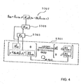
• Fig. 4 is an explanatory view of a square root array algorithm of Theorem 2.
• Fig. 5 is a flowchart of a fast algorithm of Theorem 3, which is numerically stable.
• Fig. 6 is a view showing values of an impulse response {h_i}_i=0 ²³ _.
• Fig. 7 shows an estimation result of the impulse response by the fast algorithm of Theorem 3, which is numerically stable.
• Fig. 8 is a structural view for system estimation.
• Fig. 9 is an explanatory view of a communication system and an echo.
• Fig. 10 is a principle view of an echo canceller.
DESCRIPTION OF THE PREFERED EMBODIMENTS
• Hereinafter, embodiments of the invention will be described.
1. Explanation of Symbols
• First, main symbols used in the embodiments of the invention and whether they are known or unknown will be described.
• x_k: State vector or simply a state; unknown and this is an object of the estimation.
• x_o: Initial state; unknown.
• w_k: System noise; unknown.
• v_k: Observation noise; unknown.
• y_k: Observation signal; input of a filter and known.
• Z_k: Output signal; unknown.
• F_k: Dynamics of a system; known.
• G_k: Drive matrix; known at the time of execution.
• H_k: Observation matrix; known.
• x^_k|k: Estimated value of a state x_k at a time k, using observation signals y₀ to y_k; given by a filter equation.
• X^_k+1|k: Estimated value of a state x_k+1 at a time k+1 using the observation symbols y₀ to y_k; given by the filter equation.
• x^_0|0: Initial estimated value of a state; originally unknown, however, 0 is used for convenience.
• Σ^_k|k: Corresponds to a covariance matrix of an error of X^_k|k; given by a Riccati equation.
• Σ^_k+1|k: Corresponds to a covariance matrix of an error of x^_k+1|k; given by the Riccati equation.
• Σ^_1|0: Corresponds to a covariance matrix in an initial state; originally unknown, however, ε₀I is used for convenience.
• K_s,k: Filter gain; obtained from a matrix Σ^_k|k-1.
• ρ: Forgetting factor; in the case of Theorems 1 to 3, when γ_f is determined, it is automatically determined by ρ = 1 - χ(γ_f).
• e_f,i: Filter error
• R_e,k: Auxiliary variable
• Incidentally, "^" and "v" placed above the symbol mean estimated values. Besides, "~" , "-" , "U" and the like are symbols added for convenience. Although these symbols are placed at the upper right of characters for input convenience, as indicated in mathematical expressions, they are the same as those placed directly above the characters. Besides, x, w, H, G, K, R, Σ and the like are matrixes and should be expressed by thick letters as indicated in the mathematical expressions, however, they are expressed in normal letters for input convenience.
2. Hardware and Program for System Estimation
• The system estimation or the system estimation device and system can be provided by a system estimation program for causing a computer to execute respective procedures, a computer readable recording medium recording the system estimation program, a program product including the system estimation program and capable of being loaded into an internal memory of a computer, a computer, such as a server, including the program, and the like.
• Fig. 1 is a structural view of hardware of this embodiment.
• This hardware includes a processing section 101 which is a central processing unit (CPU), an input section 102, an output section 103, a display section 104 and a storage section 105. Besides, the processing section 101, the input section 102, the output section 103, the display section 104 and the storage section 105 are connected by suitable connection means such as a star or a bus. Known data indicated in "1. Explanation of Symbols" and subjected to the system estimation are stored in the storage section 105 as the need arises. Besides, unknown and known data, calculated data relating to the hyper H_∞ filter, and other data are written and/or read by the processing section 101 as the need arises.
3. Hyper H_∞ Filter by Which Forgetting Factor Can Be Optimally Determined (Theorem 1)
• Consideration is given to a state space model as indicated by following expressions. $$x_{k+1}=F_k{x}_k+G_k{w}_k,\hspace{0.17em}{w}_k,x_k\in {ℛ}^N$$

  

  $$y_k=H_k{x}_k+v_k,\hspace{0.17em}{y}_k,v_k\in ℛ$$

  

  $$z_k=H_k{x}_k,\hspace{0.17em}{z}_k\in ℛ,\hspace{0.17em}{H}_k\in {\mathrm{<figure-callout\; id="1"\; label="R"\; filenames="imgf0003.png,imgf0004.png"\; state="\{\{state\}\}">ℛ</figure-callout>}}^{1\times N},\hspace{0.17em}k=0,1,\dots ,L$$

  
• An H_∞ evaluation criterion as indicated by the following expression is proposed for the state space model as described above.

  
• A state estimated value x^_k|k (or an output estimated value z^v _k|k) to satisfy this H_∞ evaluation criterion is given by a hyper H_∞ filter of level γ_f:

  

  $${\widehat{x}}_{k|k}=F_{k-1}{\widehat{x}}_{k-1|k-1}+K_{s,k}\left(y_k-H_k{F}_{k-1}{\widehat{x}}_{k-1|k-1}\right)$$

  

  $$K_{s,k}={\widehat{\Sigma }}_{k|k-1}{H}_k^T\cdot {\left(H_k{\widehat{\Sigma }}_{k|k-1}{H}_k^T+\rho \right)}^{-1}$$

  

  $$\begin{array}{l}{\widehat{\Sigma }}_{k|k}={\widehat{\Sigma }}_{k|k-1}-{\widehat{\Sigma }}_{k|k-1}{C}_k^T{R}_{e,k}^{-1}{C}_k{\widehat{\Sigma }}_{k|k-1}\\ {\widehat{\Sigma }}_{k+1|k}=\left(F_k{\widehat{\Sigma }}_{k|k}{F}_k^T\right)/\rho \end{array}\}$$

  

  
  where,

  

  $$\begin{array}{c}{R}_{e,k}=R_k+C_k{\widehat{\Sigma }}_{k|k-1}{C}_k^T,\hspace{0.17em}{R}_k=\left[\begin{array}{cc}\mathrm{<figure-callout\; id="0"\; label="\rho "\; filenames="imgf0002.png,imgf0003.png"\; state="\{\{state\}\}">\rho </figure-callout>}& 0\\ 0& -\rho {\gamma }_f^2\end{array}\right],\hspace{0.17em}{C}_k=\left[\begin{array}{c}{H}_k\\ H_k\end{array}\right]\end{array}$$

  

  $$0<\rho =1-\chi \left({\gamma }_f\right)\le 1,\hspace{0.17em}{\gamma }_f>1$$

  

  
  Incidentally, expression (11) denotes a filter equation, expression (12) denotes a filter gain, and expression (13) denotes a Riccati equation.
• Besides, a drive matrix G_k is generated as follows. $$G_k{G}_k^T=\frac{\chi \left({\gamma }_f\right)}{\rho }{F}_k{\widehat{\Sigma }}_{k|k}{F}_k^T$$

  
• Besides, in order to improve the tracking capacity of the foregoing H_∞ filter, the upper limit value γ_f is set to be as small as possible so as to satisfy the following existence condition. $${\widehat{\Sigma }}_{i|i}^{-1}={\widehat{\Sigma }}_{i|i-1}^{-1}+\frac{1-{\gamma }_f^{-2}}{\rho }{H}_i^T{H}_i>0,\hspace{0.17em}i=0,\dots ,k$$

  

  
  Where, χ(γ_f) is a monotonically damping function of γ_f, which satisfies χ(1) = 1 and χ(∞) = 0.
• The feature of Theorem 1 is that the generation of robustness in the state estimation and the optimization of the forgetting factor ρ are simultaneously performed.
• Fig. 2 shows a flowchart concerning the generation of robustness of the H_∞ filter and the optimization of the forgetting factor ρ. Here,
  block "EXC > 0": an existence condition of the H_∞ filter, and
  Δγ: a positive real number.
• First, the processing section 101 reads out or inputs the upper limit value γ_f from the storage section 105 or the input section 102 (S101). In this example, γ_f » 1 is given. The processing section 101 determines the forgetting factor ρ by expression (15) (S103). Thereafter, the processing section 101 executes the hyper H_∞ filter of expression (10) to expression (13) based on the forgetting factor ρ (S105). The processing section 101 calculates expression (17) (or the right side (this is made EXC) of after-mentioned expression (18)) (S107), and when the existence condition is satisfied at all times (S109), γ_f is decreased by Δγ, and the same processing is repeated (S111). On the other hand, when the existence condition is not satisfied at a certain γ_f (S109), what is obtained by adding Δγ to the γ_f is made the optimal value γ_f ^op of γ_f, and is outputted to the output section 103 and/or stored into the storage section 105 (S113). Incidentally, in this example, although Δγ is added, a previously set value other than that may be added. This optimization process is called a γ-iteration. Incidentally, the processing section 101 may store a suitable intermediate value and a final value obtained at respective steps, such as the H_∞ filter calculation step S105 and the existence condition calculation step S107, into the storage section 105 as the need arises, and may read them from the storage section 105.
• When the hyper H_∞ filter satisfies the existence condition, the inequality of expression (9) is always satisfied. Thus, in the case where the disturbance energy of the denominator of expression (9) is limited, the total sum of the square estimated error of the numerator of expression (9) becomes bounded, and the estimated error after a certain time becomes 0. This means that when γ_f can be made smaller, the estimated value x^k|k can quickly follow the change of the state x_k.
• Here, attention should be given to the fact that the algorithm of the hyper H_∞ filter of Theorem 1 is different from that of the normal H_∞ filter. Besides, when γ_f → ∞, then ρ = 1 and G_k = 0, and the algorithm of the H_∞ filter of Theorem 1 coincides with the algorithm of the Kalman filter.
• Fig. 3 is a flowchart of the algorithm of the (hyper) H_∞ filter (S105) in Fig. 2.
• The hyper H_∞ filtering algorithm can be summarized as follows.
• [Step S201] The processing section 101 reads out the initial condition of a recursive expression from the storage section 105 or inputs the initial condition from the input section 102, and determines it as indicated in the figure. Incidentally, L denotes a previously fixed maximum data number.
• [Step S203] The processing section 101 compares the time k with the maximum data number L. When the time k is larger than the maximum data number, the processing section 101 ends the processing, and when not larger, advance is made to a next step. (If unnecessary, the conditional sentence can be removed. Alternatively, restart may be made as the need arises.)
• [Step S205] The processing section 101 calculates a filter gain K_s,k by using expression (12).
• [Step S207] The processing section 101 updates the filter equation of the hyper H_∞ filter of expression (11).
• [Step S209] The processing section 101 calculates terms Σ^_k|k, Σ^_k+1|k corresponding to the covariance matrix of an error by using the Riccati equation of expression (13).
• [Step S211] The time k is made to advance (k = k + 1), return is made to step S203, and continuation is made as long as data exists.
• Incidentally, the processing section 101 may store a suitable intermediate value, a final value, a value of the existence condition and the like obtained at the respective steps, such as the H_∞ filter calculation steps S205 to S209, into the storage section 105 as the need arises, or may read them from the storage section 105.
(Scalar Existence Condition)
• The amount of calculation O(N²) was necessary for the judgment of the existence condition of expression (17). However, when the following condition is used, the existence of the H_∞ filter of Theorem 1, that is, expression (9) can be verified by the amount of calculation O(N).
Corollary 1: Scalar existence condition
• When the following existence condition is used, the existence of the hyper H_∞ filter can be judged by the amount of calculation O(N). $$-\varrho {\widehat{\Xi }}_i+\rho {\gamma }_{\mathrm{<figure-callout\; id="2"\; label="f"\; filenames="imgf0008.png"\; state="\{\{state\}\}">f</figure-callout>}}^2>0,\hspace{0.17em}i=0,\cdots ,k$$

  

  
  Here; $$\varrho =1-{\mathrm{<figure-callout\; id="2"\; label="\gamma \; f"\; filenames="imgf0008.png"\; state="\{\{state\}\}">\gamma </figure-callout>}}_f^{},\hspace{0.17em}{\widehat{\Xi }}_i=\frac{\rho H_i{K}_{s,i}}{1-H_i{K}_{s,i}},\hspace{0.17em}\rho =1-\chi \left({\gamma }_f\right)$$

  

  
  Where, K_s,i denotes the filter gain obtained in expression (12).
(Proof)
• Hereinafter, the proof of the system 1 will be described.
• When a characteristic equation $$\left|\lambda I-R_{e,k}\right|=\left|\begin{array}{cc}\lambda -\left(\rho +H_k{\widehat{\Sigma }}_{k|k-1}{H}_k^T\right)& -H_k{\widehat{\Sigma }}_{k|k-1}{H}_k^T\\ -H_k{\widehat{\Sigma }}_{k|k}{H}_k^T& \lambda -\left(-\mathrm{<figure-callout\; id="2"\; label="\rho \; \gamma \; f"\; filenames="imgf0008.png"\; state="\{\{state\}\}">\rho </figure-callout>}{\gamma }_f^{}{}_2^{}+H_k{\widehat{\Sigma }}_{k|k-1}{H}_k^T\right)\end{array}\right|={\mathrm{<figure-callout\; id="2"\; label="\lambda "\; filenames="imgf0008.png"\; state="\{\{state\}\}">\lambda </figure-callout>}}^2-\left(2H_k{\widehat{\Sigma }}_{k|k-1}{H}_k^T+\rho \varrho \right)\lambda -{\mathrm{<figure-callout\; id="2"\; label="\rho "\; filenames="imgf0008.png"\; state="\{\{state\}\}">\rho </figure-callout>}}^2{\mathrm{<figure-callout\; id="2"\; label="\gamma \; f"\; filenames="imgf0008.png"\; state="\{\{state\}\}">\gamma </figure-callout>}}_f^{}+\rho \varrho H_k{\widehat{\Sigma }}_{k|k-1}{H}_k^T=0$$

  

  
  of a 2 × 2 matrix R_e,k is solved, an eigenvalue λ_i of R_e,k is obtained as follows. $${\lambda }_i=\frac{\Phi \pm \sqrt{{\Phi }^2-4\rho \varrho H_k{\widehat{\Sigma }}_{k|k-1}{H}_k^T+2{\mathrm{<figure-callout\; id="2"\; label="\rho "\; filenames="imgf0008.png"\; state="\{\{state\}\}">\rho </figure-callout>}}^2{\mathrm{<figure-callout\; id="2"\; label="\gamma \; f"\; filenames="imgf0008.png"\; state="\{\{state\}\}">\gamma </figure-callout>}}_f^{}}}{2}$$

  

  Where, $$\Phi =2H_k{\widehat{\Sigma }}_{k|k-1}{H}_k^T+\rho \varrho ,\hspace{0.17em}\varrho =1-{\mathrm{<figure-callout\; id="2"\; label="\gamma \; f"\; filenames="imgf0008.png"\; state="\{\{state\}\}">\gamma </figure-callout>}}_f^{}$$

  

  
  If $$-4\rho \varrho H_k{\widehat{\Sigma }}_{k|k-1}{H}_k^T+4{\mathrm{<figure-callout\; id="2"\; label="\rho "\; filenames="imgf0008.png"\; state="\{\{state\}\}">\rho </figure-callout>}}^2{\mathrm{<figure-callout\; id="2"\; label="\gamma \; f"\; filenames="imgf0008.png"\; state="\{\{state\}\}">\gamma </figure-callout>}}_f^{}>0$$

  

  
  one of two eigenvalues of the matrix R_e,k becomes positive, the other becomes negative, and the matrixes R_k and R_e,k have the same inertia. By this, when $$H_k{\widehat{\Sigma }}_{k|k-1}{H}_k^T=\frac{H_k{\tilde{K}}_{\mathrm{<figure-callout\; id="1"\; label="k"\; filenames="imgf0003.png,imgf0004.png"\; state="\{\{state\}\}">k</figure-callout>}}}{1-\frac{1-{\gamma }_f^{-2}}{\rho }{H}_k{\tilde{K}}_k},\hspace{0.17em}{H}_k{\tilde{K}}_k=\frac{\rho H_k{K}_{s,\mathrm{<figure-callout\; id="1"\; label="k"\; filenames="imgf0003.png,imgf0004.png"\; state="\{\{state\}\}">k</figure-callout>}}}{1-{\gamma }_f^{-2}{H}_k{K}_{s,k}}$$

  

  
  is used, the existence condition of expression (18) is obtained. Here, the amount of calculation of H_kK_s,k is O(N).
4. State Estimation Algorithm Which Is Numerically Stable
• Since the foregoing hyper H_∞ filter updates Σ^_k|k-1 ∈ R^n×n, the amount of calculation per unit time step becomes O(N²), that is, an arithmetic operation proportional to N² becomes necessary. Here, N denotes the dimension of the state vector x_k. Thus, as the dimension of x_k is increased, the calculation time required for execution of this filter is rapidly increased. Besides, although the error covariance matrix Σ^_k|k-1 must always have the positive definite from its property, there is a case where it has numerically the negative definite. Especially, in the case where calculation is made at single precision, this tendency becomes remarkable. At this time, it is known that the filter becomes unstable. Thus, in order to put the algorithm to practical use and to reduce the cost, the development of the state estimation algorithm which can be operated even at single precision (example: 32 bit) is desired.
• Then, next, attention is paid to $${\mathrm{R}}_{\mathrm{k}}={{\mathrm{<figure-callout\; id="1"\; label="R"\; filenames="imgf0003.png,imgf0004.png"\; state="\{\{state\}\}">R</figure-callout>}}^{1/2}}_{\mathrm{k}}{\mathrm{J}}_1{{\mathrm{<figure-callout\; id="1"\; label="R"\; filenames="imgf0003.png,imgf0004.png"\; state="\{\{state\}\}">R</figure-callout>}}^{1/2}}_{\mathrm{k}},$$

  

  $${\mathrm{R}}_{\mathrm{e},\mathrm{k}}={{\mathrm{<figure-callout\; id="1"\; label="R"\; filenames="imgf0003.png,imgf0004.png"\; state="\{\{state\}\}">R</figure-callout>}}^{1/2}}_{\mathrm{e}\mathrm{,}\mathrm{k}}{\mathrm{J}}_1{{\mathrm{<figure-callout\; id="1"\; label="R"\; filenames="imgf0003.png,imgf0004.png"\; state="\{\{state\}\}">R</figure-callout>}}^{1/2}}_{\mathrm{e}\mathrm{,}\mathrm{k}},$$

  

  and $${{\mathrm{\Sigma }}^{\widehat{\mathrm{\hspace{1em}}}}}_{\mathrm{k}|\mathrm{k}-1}={{\mathrm{\Sigma }}^{\widehat{\mathrm{\hspace{1em}}}1/2}}_{\mathrm{k}|\mathrm{k}-1}{{\mathrm{\Sigma }}^{\widehat{\mathrm{\hspace{1em}}}1/2}}_{\mathrm{k}|\mathrm{k}-1},$$

  

  
  and an H_∞ filter (square root array algorithm) of Theorem 1, which is numerically stabilized, is indicated in Theorem 2. Here, although it is assumed that F_k = I is established for simplification, it can be obtained in the same way also in the case of F_k ≠ I. Hereinafter, the hyper H_∞ filter to realize the state estimation algorithm which is numerically stable will be indicted.
• (Theorem 2) $${\widehat{x}}_{k|k}={\widehat{x}}_{k-1|k-1}+K_{s,k}\left(y_k-H_k{\widehat{x}}_{k-1|k-1}\right)$$

  

  $$K_{s,k}=H_k\left(:,1\right)/R_{e,k}\left(1,1\right),\hspace{0.17em}{K}_k={\mathrm{<figure-callout\; id="1"\; label="\rho "\; filenames="imgf0003.png,imgf0004.png"\; state="\{\{state\}\}">\rho </figure-callout>}}^{\frac{1}{2}}\left({\rho }^{-\frac{1}{2}}{K}_k{R}_{e,k}^{-\frac{1}{2}}{\mathrm{<figure-callout\; id="1"\; label="J"\; filenames="imgf0003.png,imgf0004.png"\; state="\{\{state\}\}">J</figure-callout>}}_1^{-1}\right)J_1{R}_{e,\mathrm{<figure-callout\; id="1"\; label="k"\; filenames="imgf0003.png,imgf0004.png"\; state="\{\{state\}\}">k</figure-callout>}}^{\frac{1}{2}}$$

  

  $$\left[\begin{array}{cc}{\mathrm{<figure-callout\; id="1"\; label="R\; k"\; filenames="imgf0003.png,imgf0004.png"\; state="\{\{state\}\}">R</figure-callout>}}_k^{}& C_k{\widehat{\Sigma }}_{k|k-1}^{\frac{1}{2}}\\ 0& {\rho }^{-\frac{1}{2}}{\widehat{\Sigma }}_{k|k-1}^{\frac{1}{2}}\end{array}\right]\Theta \left(k\right)=\left[\begin{array}{cc}{R}_{e,\mathrm{<figure-callout\; id="1"\; label="k"\; filenames="imgf0003.png,imgf0004.png"\; state="\{\{state\}\}">k</figure-callout>}}^{\frac{1}{2}}& 0\\ {\rho }^{-\frac{1}{2}}{K}_k{R}_{e,k}^{-\frac{1}{2}}{\mathrm{<figure-callout\; id="1"\; label="J"\; filenames="imgf0003.png,imgf0004.png"\; state="\{\{state\}\}">J</figure-callout>}}_1^{-1}& {\widehat{\Sigma }}_{k+1|\mathrm{<figure-callout\; id="1"\; label="k"\; filenames="imgf0003.png,imgf0004.png"\; state="\{\{state\}\}">k</figure-callout>}}^{\frac{1}{2}}\end{array}\right]$$

  

  
  Where,

  

  Θ(k) denotes a J-unitary matrix, that is, Θ(k)JΘ(k)^T = J is satisfied, J = (J₁ ⊕ I), and I is a unit matrix. Besides, K_k(:,1) indicates the column vector of the first column of the matrix K_k.
• Incidentally, in expressions (21) and (22), J₁ ^-1 and J₁ can be deleted.
• Fig. 4 is an explanatory view of the square root array algorithm of Theorem 2. This calculation algorithm can be used in the calculation (S105) of the H_∞ filter in the flowchart of Theorem 1 shown in Fig. 2.
• In this estimation algorithm, instead of obtaining Σ^_k|k-1 by a Riccati type update expression, its factor matrix Σ^^1/2 _k|k-1 ∈ R^N×N (square root matrix of Σ^_k|k-1) is obtained by the update expression based on the J-unitary transformation. From a 1-1 block matrix and a 2-1 block matrix generated at this time, the filter gain K_s,k is obtained as shown in the figure. Thus, Σ^_k|k-1 = Σ^^1/2 _k|k-1 Σ^^1/2 _k|k-1 > 0 is established, the positive definite property of Σ^_k|k-1 is ensured, and it can be numerically stabilized. Incidentally, a computational complexity of the H_∞ filter of Theorem 2 per unit step remains O(N²).
• Incidentally, in Fig. 4, J₁ ^-1 can be deleted.
• First, the processing section 101 reads out terms contained in the respective elements of the left-side equations of expression (22) from the storage section 105 or obtains them from the internal memory or the like, and executes the J-unitary transformation (S301). The processing section 101 calculates system gains K_k and K_s,k from the elements of the right-side equations of the obtained expression (22) based on expression (21) (S303, S305). The processing section 101 calculates the state estimated value x^_k|k based on expression (20) (S307).
5. Numerically Stable Fast Algorithm for State Estimation
• As described above, a computational complexity of the H_∞ filter of Theorem 2 per unit step remains O(N²). Then, as a countermeasure for the complexity, by using that when H _k = H _k+1Ψ, H _k = [u(k) , ··· , u(0), 0, ··· , 0], a covariance matrix Σ _k+1k|k of one step prediction error of x _k = [x^T _k, 0^T]^T satisfies $${\underset{‾}{\Sigma }}_{k+1|k}-\Psi {\underset{‾}{\Sigma }}_{k|k-1}{\Psi }^T=-{\underset{‾}{L}}_k{R}_{r,k}^{-1}{\underset{‾}{L}}_k^T,\hspace{0.17em}{\underset{‾}{L}}_k=\left[\begin{array}{c}{\tilde{L}}_k\\ 0\end{array}\right]$$

  

  consideration is given to updating L _k (that is, L^~ _x) with a low dimension instead of Σ _k+1|k· Here, when attention is paid to R_r,k = R^1/2 _r,k SR^1/2 _r,k' next Theorem 3 can be obtained.
• (Theorem 3) $${\widehat{x}}_{k|k}={\widehat{x}}_{k-1|k-1}+{\bar{K}}_{s,k}\left(y_k-H_k{\widehat{x}}_{k-1|k-1}\right)$$

  

  $${\bar{K}}_{s,k}={\bar{K}}_k\left(:,1\right)/R_{e,k}\left(1,1\right),\hspace{0.17em}{\bar{K}}_k={\mathrm{<figure-callout\; id="1"\; label="\rho "\; filenames="imgf0003.png,imgf0004.png"\; state="\{\{state\}\}">\rho </figure-callout>}}^{\frac{1}{2}}\left({\bar{K}}_k{R}_{e,k}^{-\frac{1}{2}}\right)R_{e,\mathrm{<figure-callout\; id="1"\; label="k"\; filenames="imgf0003.png,imgf0004.png"\; state="\{\{state\}\}">k</figure-callout>}}^{\frac{1}{2}}$$

  

  

  Here, Θ(k) denotes an arbitrary J-unitary matrix, and C_k = C_k+1Ψ is established.
  Where,

  
• Incidentally, the proof of Theorem 3 will be described later.
• The above expression can be arranged with respect to K_k instead of K^- _k(= P^-1/2K_k).
• Further, when the following J-unitary matrix $$\mathrm{\Theta }\left(k\right)=\left(J_1{R}_{e,\mathrm{<figure-callout\; id="1"\; label="k"\; filenames="imgf0003.png,imgf0004.png"\; state="\{\{state\}\}">k</figure-callout>}}^{\frac{1}{2}}\oplus -R_{r,\mathrm{<figure-callout\; id="1"\; label="k"\; filenames="imgf0003.png,imgf0004.png"\; state="\{\{state\}\}">k</figure-callout>}}^{\frac{1}{2}}\right)\Sigma \left(k\right)\left(R_{e,k+1}^{-\frac{1}{2}}{\mathrm{<figure-callout\; id="1"\; label="J"\; filenames="imgf0003.png,imgf0004.png"\; state="\{\{state\}\}">J</figure-callout>}}_1^{-1}\oplus -R_{r,k+1}^{-\frac{1}{2}}\right)$$

  

  
  is used, a fast state estimation algorithm of Theorem 4 can be obtained. Where, Ψ denotes a shift matrix.
• (Theorem 4) $${\widehat{x}}_{k|k}={\widehat{x}}_{k-1|k-1}+K_{s,k}\left(y_k-H_k{\widehat{x}}_{k-1|k-1}\right)$$

  

  $$K_{s,k}={\mathrm{<figure-callout\; id="1"\; label="\rho "\; filenames="imgf0003.png,imgf0004.png"\; state="\{\{state\}\}">\rho </figure-callout>}}^{\frac{1}{2}}{\bar{K}}_k\left(:,1\right)/R_{e,k}\left(1,1\right)$$

  

  

  

  

  

  Where,

  

  diag [.] denotes a diagonal matrix, and R_e,k+1(1,1) denotes a 1-1 element of the matrix R_e,k+1. Besides, the above expression can be arranged with respect to K_k instead of K^- _k.
• In the fast algorithm, since the filter gain K_s,k is obtained by the update of L^~ _k ∈ R^(N+1)×2 in the following factoring $${\underset{‾}{\Sigma }}_{k+1|k}-\Psi {\underset{‾}{\Sigma }}_{k|k-1}{\Psi }^T=-{\underset{‾}{L}}_k{R}_{r,k}^{-1}{\underset{‾}{L}}_k^T$$

  

  
  O(N+1) is sufficient for the amount of calculation per unit step. Here, attention should be paid to the following expression.

  
• Fig. 5 is a flowchart of a numerically stable fast algorithm of Theorem 3. The fast algorithm is incorporated in the calculation step (S105) of the H_∞ filter of Fig. 2, and is optimized by the γ-iteration. Thus, during a period in which the existence condition is satisfied, γ_f is gradually decreased, however, at the time point when it comes to be unsatisfied, γ_i is increased as indicated in the figure.
• The H_∞ filtering algorithm can be summarized as follows.
• [Step S401] The processing section 101 determines an initial condition of the recursive expression as indicated in the figure. Incidentally, L denotes a maximum data number.
• [Step S403] The processing section 101 compares the time k with the maximum data number L. When the time k is larger than the maximum data number, the processing section 101 ends the processing, and when not larger, advance is made to a next step. (When unnecessary, the conditional sentence can be removed. Alternatively, restart is made.)
• [Step S405] The processing section 101 recursively calculates a term K_k+1 corresponding to a filter gain by using expressions (27) and (31).
• [Step S406] The processing section 101 recursively calculates R_e,k+1 by using expression (29).
• [Step S407] The processing section 101 further calculates K_s,k by using expressions (26) and (31).
• [Step S409] The processing section 101 judges the existence condition EXC > 0 here, and when the existence condition is satisfied, advance is made to step S411.
• [Step S413] On the other hand, when the existence condition is not satisfied at step S409, the processing section 101 increases γ_f, and return is made to step S401.
• [Step S411] The processing section 101 updates the filter equation of the H_∞ filter of expression (25).
• [Step S415] The processing section 101 recursively calculates R_r,k+1 by using expression (30). Besides, the processing section 101 recursively calculates L^~ _k+1 by using expressions (28) and (31) .
• [Step S419] The processing section 101 advances the time k (k = k+1), returns to step S403, and continues as long as data exists.
• Incidentally, the processing section 101 may store a suitable intermediate value and a final value obtained at the respective steps, such as the H_∞ filter calculation steps S405 to S415 and the calculation step S409 of the existence condition, into the storage section 105 as the need arises, and may read them from the storage section 105.
6. Echo Canceller
• Next, a mathematical model of an echo canceling problem is generated.
• First, when consideration is given to the fact that a received signal {u_k} becomes an input signal to an echo path, by a (time-varying) impulse response {h_i[k]} of the echo path, an observed value {y_k} of an echo {d_k} is expressed by the following expression. $$y_k=d_k+v_k={\displaystyle \sum _{i=0}^{N-1}{h}_i\left[k\right]u_{k-i}}+v_k,\hspace{0.17em}k=0,1,2,\cdots$$

  

  
  Here, u_k and y_k respectively denote the received signal and the echo at a time t_k (= kT; T is a sampling period), v_k denotes circuit noise having a mean value of 0 at the time t_k, h_i[k], i = 0, ·· ·, N-1 denotes a time-varying impulse response, and the tap number N thereof is known. At this time, when estimated values {h^_i[k]} of the impulse response are obtained every moment, a pseudo-echo as indicated below can be generated by using that. $${\widehat{d}}_k={\displaystyle \sum _{i=0}^{N-1}{\widehat{h}}_i\left[k\right]u_{k-i}},\hspace{0.17em}k=0,1,2,\cdots$$

  

  
  When this is subtracted from the echo (y_k - d^_k ≈ 0), the echo can be cancelled. Where, it is assumed that if k-i < 0, then u_k-1 = 0.
• From the above, the problem can be reduced to the problem of successively estimating the impulse response {h_i[k]} of the echo path from the received signal {u_k} and the echo {y_κ} which can be directly observed.
• In general, in order to apply the H_∞ filter to the echo canceller, first, expression (32) must be expressed by a state space model including a state equation and an observation equation. Then, since the problem is to estimate the impulse response {h_i[k]}, when {h_i[k]} is made a state variable x_k, and a variance of about W_k is allowed, the following state space model can be established for the echo path. $$x_{k+1}=x_k+G_k{w}_k,\hspace{0.17em}{x}_k,w_k\in {ℛ}^N$$

  

  $$y_k=H_k{x}_k+v_k,\hspace{0.17em}{y}_k,v_k\in ℛ$$

  

  $$z_k=H_k{x}_k,\hspace{0.17em}{z}_k\in ℛ,\hspace{0.17em}{H}_k\in {\mathrm{<figure-callout\; id="1"\; label="R"\; filenames="imgf0003.png,imgf0004.png"\; state="\{\{state\}\}">ℛ</figure-callout>}}^{1\times N}$$

  

  
  Where, $$x_k={\left[h_0\left[k\right],\cdots ,h_{N-1}\left[k\right]\right]}^T,\hspace{0.17em}{w}_k={\left[w_k\left(1\right),\cdots ,w_k\left(N\right)\right]}^T$$

  

  $$H_k=\left[u_k,\cdots ,u_{k-N+1}\right]$$

  
• The hyper and fast H_∞ filtering algorithms to the state space model as stated above is as described before. Besides, at the estimation of the impulse response, when the generation of a transmission signal is detected, the estimation is generally suspended during that.
7. Evaluation to Impulse Response (Confirmation of Operation)
• With respect to the case where the impulse response of the echo pulse is temporally invariable (h_i[k] = h_i), and the tap number N is 48 , the operation of the fast algorithm is confirmed by using a simulation. $$y_k={\displaystyle \sum _{i=0}^{47}{h}_i{u}_{k-i}}+v_k$$

  

  
  Incidentally, Fig. 6 is a view showing values of the impulse response {h_i} here.
• Here, the value shown in the figure are used for the impulse response {h_i}_i=0 ²³, and the other {h_i}_i=24 ⁴⁷ is made 0. Besides, it is assumed that v_k is stationary Gaussian white noise having a mean value of 0 and variance σ_v ² = 1.0 × 10^-6, and the sampling period T is made 1.0 for convenience.
• Besides, the received signal {u_k} is approximated by a secondary AR model as follows. $${\mathrm{u}}_{\mathrm{k}}={\mathrm{\alpha }}_1{\mathrm{u}}_{\mathrm{k}-1}+{\mathrm{\alpha }}_2{\mathrm{u}}_{\mathrm{k}-2}+\mathrm{w}{}_{\mathrm{k}}\prime$$

  

  
  Where, α₁ = 0.7 and α₂ = 0.1 are assumed, and w_k' denotes stationary Gaussian white noise having a means value of 0 and variance σ_w' ² = 0.04.
(Estimation Result of Impulse Response)
• Fig. 7 shows an estimation result of the impulse response by the numerically stable fast algorithm of Theorem 3. Here, the vertical axis of Fig. 7(b) indicates $$\mathrm{\surd }\left\{{\sum _{\mathrm{i}=0}}^{47}{({\mathrm{h}}_{\mathrm{i}}-{{\mathrm{x}}^{-}}_{\mathrm{k}}(\mathrm{i}+1))}^2\right\}\mathrm{.}$$

  
• By this, it is understood that the estimation can be excellently performed by the fast algorithm. Where, ρ = 1- χ(γ_f), χ(γ_f) = γ_f ^-2, x^_0|0 = 0 and Σ^_0|0 = 20I were assumed, and the calculation was performed at double precision. Besides, while the existence condition is confirmed, γ_f = 5.5 was set.
8. Proof of Theorem 8-1. Proof of Theorem 2
• When the following expression: $$\left[\begin{array}{cc}{\mathrm{<figure-callout\; id="1"\; label="R\; k"\; filenames="imgf0003.png,imgf0004.png"\; state="\{\{state\}\}">R</figure-callout>}}_k^{}& C_k{\widehat{\Sigma }}_{k|k-1}^{\frac{1}{2}}\\ 0& {\rho }^{-\frac{1}{2}}{\widehat{\Sigma }}_{k|k-1}^{\frac{1}{2}}\end{array}\right]J\left[\begin{array}{cc}{\mathrm{<figure-callout\; id="1"\; label="R\; k"\; filenames="imgf0003.png,imgf0004.png"\; state="\{\{state\}\}">R</figure-callout>}}_k^{}& 0\\ {\widehat{\Sigma }}_{k|k-1}^{\frac{1}{2}}{C}_k^T& {\rho }^{-\frac{1}{2}}{\widehat{\Sigma }}_{k|k-1}^{\frac{1}{2}}\end{array}\right]=\left[\begin{array}{cc}{R}_{e,\mathrm{<figure-callout\; id="1"\; label="k"\; filenames="imgf0003.png,imgf0004.png"\; state="\{\{state\}\}">k</figure-callout>}}^{\frac{1}{2}}& 0\\ {\rho }^{-\frac{1}{2}}{K}_k{R}_{e,k}^{-\frac{1}{2}}{\mathrm{<figure-callout\; id="1"\; label="J"\; filenames="imgf0003.png,imgf0004.png"\; state="\{\{state\}\}">J</figure-callout>}}_1^{-1}& {\widehat{\Sigma }}_{k+1|\mathrm{<figure-callout\; id="1"\; label="k"\; filenames="imgf0003.png,imgf0004.png"\; state="\{\{state\}\}">k</figure-callout>}}^{\frac{1}{2}}\end{array}\right]J\left[\begin{array}{cc}{R}_{e,\mathrm{<figure-callout\; id="1"\; label="k"\; filenames="imgf0003.png,imgf0004.png"\; state="\{\{state\}\}">k</figure-callout>}}^{\frac{1}{2}}& {\rho }^{-\frac{1}{2}}{\mathrm{<figure-callout\; id="1"\; label="J"\; filenames="imgf0003.png,imgf0004.png"\; state="\{\{state\}\}">J</figure-callout>}}_1^{-1}{R}_{e,k}^{-\frac{1}{2}}{\mathrm{<figure-callout\; id="0"\; label="K\; k\; T"\; filenames="imgf0002.png,imgf0003.png"\; state="\{\{state\}\}">K</figure-callout>}}_{kT}^{}\\ 0& {\widehat{\Sigma }}_{k+1|\mathrm{<figure-callout\; id="1"\; label="k"\; filenames="imgf0003.png,imgf0004.png"\; state="\{\{state\}\}">k</figure-callout>}}^{\frac{1}{2}}\end{array}\right]$$

  

  
  is established, following expressions are obtained by comparing the respective terms of 2 × 2 block matrixes of both sides. $$R_{e,k}=R_k+C_k{\widehat{\Sigma }}_{k|k-1}{C}_k^T$$

  

  $${\mathit{K}}_k={\widehat{\Sigma }}_{k|k-1}{C}_k^T$$

  

  $${\widehat{\Sigma }}_{k+1|k}+{\rho }^{-1}{K}_k{R}_{e,k}^{-1}{K}_k^T={\rho }^{-1}{\widehat{\Sigma }}_{k|k-1}$$

  
• This is coincident with the Riccati equation of expression (13) at F_k = I of Theorem 1. Where, $$J=\left({\mathrm{<figure-callout\; id="1"\; label="J"\; filenames="imgf0003.png,imgf0004.png"\; state="\{\{state\}\}">J</figure-callout>}}_1\oplus I\right),\hspace{0.17em}{\mathrm{<figure-callout\; id="1"\; label="J"\; filenames="imgf0003.png,imgf0004.png"\; state="\{\{state\}\}">J</figure-callout>}}_1=\left[\begin{array}{cc}1& 0\\ 0& -1\end{array}\right],\hspace{0.17em}{C}_k=\left[\begin{array}{c}{H}_k\\ H_k\end{array}\right]$$

  
• On the other hand, when AJA^T = BJB^T is established, B can be expressed as B = AΘ(k) by using the J-unitary matrix Θ(K). Thus, from expression (40), the Riccati equation of Theorem 1 is equivalent to the following expression. $$\left[\begin{array}{cc}{R}_{e,\mathrm{<figure-callout\; id="1"\; label="k"\; filenames="imgf0003.png,imgf0004.png"\; state="\{\{state\}\}">k</figure-callout>}}^{\frac{1}{2}}& 0\\ {\rho }^{-\frac{1}{2}}{K}_k{R}_{e,k}^{-\frac{1}{2}}{\mathrm{<figure-callout\; id="1"\; label="J"\; filenames="imgf0003.png,imgf0004.png"\; state="\{\{state\}\}">J</figure-callout>}}_1^{-1}& {\widehat{\Sigma }}_{k+1|\mathrm{<figure-callout\; id="1"\; label="k"\; filenames="imgf0003.png,imgf0004.png"\; state="\{\{state\}\}">k</figure-callout>}}^{\frac{1}{2}}\end{array}\right]=\left[\begin{array}{cc}{\mathrm{<figure-callout\; id="1"\; label="R\; k"\; filenames="imgf0003.png,imgf0004.png"\; state="\{\{state\}\}">R</figure-callout>}}_k^{}& C_k{\widehat{\Sigma }}_{k|k-1}^{\frac{1}{2}}\\ 0& {\rho }^{-\frac{1}{2}}{\widehat{\Sigma }}_{k|k-1}^{\frac{1}{2}}\end{array}\right]\mathrm{\Theta }\left(k\right)$$

  
• Incidentally, in expressions (40) and (45), J₁ ^-1 can be deleted.
8-2. Proof of Theorem 3
• It is assumed that there is a J-unitary matrix Θ(k) which performs block triangulation as follows.

  

  At this time, when both sides J = (J₁⊕-S) - norm of the above expression are compared, X, Y and Z of the left side can be determined as follows. Where, S denote a diagonal matrix in which diagonal elements take 1 or -1. (1,1)-Block matrix

  

  Thus, $X=R_{e,k+1}^{\frac{1}{2}}$

  

  is obtained from $R_{e,k+1}=R_{e,k+1}^{\frac{1}{2}}{J}_1{R}_{e,k+1}^{\frac{1}{2}},\hspace{0.17em}{R}_{k+1}=R_k.$

  

  Here, attention should be paid to the fact that

  

  is established.
(2,1)-Block matrix
• 

  By this, $Y=\left[\begin{array}{c}{\bar{K}}_{k+1}\\ 0\end{array}\right]R_{e,k+1}^{-\frac{1}{2}}{\mathrm{<figure-callout\; id="1"\; label="J"\; filenames="imgf0003.png,imgf0004.png"\; state="\{\{state\}\}">J</figure-callout>}}_1$

  

  is obtained.
  Where,

  
(2,2)-Block Matrix
• 

  By this,

  

  and $Z={\tilde{L}}_{k+1}{R}_{r,k+1}^{-\frac{1}{2}}$

  

  is obtained.
8-3. Proof of Theorem 4
• When an observation matrix H_k has a shift characteristic and J = (J₁ ⊕ - S),
  the following relational expression is obtained by a similar method to Theorem 2.

  

  Where,

  

  Where, Σ(k) ^T (R _e,k ⊕ -R _r,k ) Σ(k) = (R _e,k+1 ⊕ -R _r,k+1)
  and R_r,k+1 is determined so that Σ(k)^T (R_e,k ⊕ - R_r,k)Σ(k) = (R_e,k+1 ⊕ - R_r,k+1) is established. Next, when an update expression of R_r,k+1 is newly added to the third line of expression (46), the following expression is finally obtained.

  
• From the correspondence of the respective terms of 3 × 2 block matrixes of both sides, the following update expression of a gain matrix K^- _k is obtained.

  

  

  

  
Industrial Applicability
• In general, in a normal civil communication equipment or the like, calculation is often performed at single precision in view of the cost and speed. Thus, as the practical state estimation algorithm, the present invention would have effects in various industrial fields. Besides, the invention can be applied to an echo canceller in a communication system or a sound system, sound field reproduction, noise control and the like.

Claims (17)

1. A system estimation method for making state estimation robust and optimizing a forgetting factor ρ simultaneously in an estimation algorithm, in which
   for a state space model expressed by following expressions: $${\mathrm{x}}_{\mathrm{k}+1}={\mathrm{F}}_{\mathrm{k}}{\mathrm{x}}_{\mathrm{k}}+{\mathrm{G}}_{\mathrm{k}}{\mathrm{w}}_{\mathrm{k}}$$

   

   $${\mathrm{y}}_{\mathrm{k}}={\mathrm{H}}_{\mathrm{k}}{\mathrm{x}}_{\mathrm{k}}+{\mathrm{v}}_{\mathrm{k}}$$

   

   $${\mathrm{z}}_{\mathrm{k}}={\mathrm{H}}_{\mathrm{k}}{\mathrm{x}}_{\mathrm{k}}$$

   

   
   here,

   x_k: a state vector or simply a state,

   w_k: a system noise,

   v_k: an observation noise,

   y_k: an observation signal,

   z_k: an output signal,

   F_k: dynamics of a system, and

   G_k: a drive matrix,

   a maximum energy gain to a filter error from a disturbance weighted with the forgetting factor ρ as an evaluation criterion is suppressed to be smaller than a term corresponding to a previously given upper limit value γ_f, and
   the system estimation method comprises:

   a step at which a processing section inputs the upper limit value γ_f, the observation signal y_k as an input of a filter and a value including an observation matrix H_k from a storage section or an input section;

   a step at which the processing section determines the forgetting factor ρ relevant to the state space model in accordance with the upper limit value γ_f;

   a step at which the processing section reads out an initial value or a value including the observation matrix H_k at a time from the storage section and uses the forgetting factor ρ to execute a hyper H_∞ filter expressed by a following expression: $${{\mathrm{x}}^{\widehat{\mathrm{\hspace{1em}}}}}_{\mathrm{k}|\mathrm{k}}={\mathrm{F}}_{\mathrm{k}-1}{{\mathrm{x}}^{\widehat{\mathrm{\hspace{1em}}}}}_{\mathrm{k}-1|\mathrm{k}-1}+{\mathrm{K}}_{\mathrm{s},\mathrm{k}}\left({\mathrm{y}}_{\mathrm{k}}-{\mathrm{H}}_{\mathrm{k}}{\mathrm{F}}_{\mathrm{k}-1}{{\mathrm{x}}^{\widehat{\mathrm{\hspace{1em}}}}}_{\mathrm{k}-1|\mathrm{k}-1}\right)$$

   

   here,

   x^_k|k; an estimated value of a state x_k at a time k using observation signals y₀ to y_k,

   K_s,k; a filter gain,

   a step at which the processing section stores an obtained value relating to the hyper H_∞ filter into the storage section;

   a step at which the processing section calculates an existence condition based on the upper limit value γ_f and the forgetting factor ρ by the obtained observation matrix H_i or the observation matrix H_i and the filter gain K_s,i, and

   a step at which the processing section sets the upper limit value to be small within a range where the existence condition is satisfied at each time and stores the value into the storage section, by decreasing the upper limit value γ_f and repeating the step of executing the hyper H_∞ filter.
2. The system estimation method according to claim 1,
   wherein the processing section calculates the existence condition in accordance with a following expression: $${\widehat{\Sigma }}_{i|i}^{-1}={\widehat{\Sigma }}_{i|i-1}^{-1}+\frac{1-{\gamma }_f^{-2}}{\rho }{H}_i^T{H}_i>0,\hspace{0.17em}i=0,\dots ,k$$

   
3. The system estimation method according to claim 1,
   wherein the processing section calculates the existence condition in accordance with a following expression: $$-\varrho {\widehat{\Xi }}_i+\rho {\gamma }_f^2>0,\hspace{0.17em}i=0,\cdots ,k$$

   

   
   here, $$\varrho =1-{\gamma }_f^2,\hspace{0.17em}{\widehat{\mathrm{\Xi }}}_i=\frac{\rho H_i{K}_{s,i}}{1-H_i{K}_{s,i}},\hspace{0.17em}\rho =1-\chi \left({\gamma }_f\right)$$

   
4. The system estimation method according to claim 1, wherein the forgetting factor ρ and the upper limit value γ_f have a following relation:
   0 < ρ = 1 - χ(γ_f ) ≤ 1, where χ(γ_f) denotes a monotonically damping function of γ_f to satisfy χ(1) = 1 and χ(∞) = 0.
5. The system estimation method according to claim 1, wherein at the step of executing the hyper H_∞ filter,
   the processing section obtains the filter gain K_s,k by following expressions:

   

   $${\widehat{x}}_{k|k}=F_{k-1}{\widehat{x}}_{k-1|k-1}+K_{s,k}\left(y_k-H_k{F}_{k-1}{\widehat{x}}_{k-1|k-1}\right)$$

   

   $$K_{s,k}={\widehat{\Sigma }}_{k|k-1}{H}_k^T\cdot {\left(H_k{\widehat{\Sigma }}_{k|k-1}{H}_k^T+\rho \right)}^{-1}$$

   

   $$\begin{array}{l}{\widehat{\Sigma }}_{k|k}={\widehat{\Sigma }}_{k|k-1}-{\widehat{\Sigma }}_{k|k-1}{C}_k^T{R}_{e,k}^{-1}{C}_k{\widehat{\Sigma }}_{k|k-1}\\ {\widehat{\Sigma }}_{k+1|k}=\left(F_k{\widehat{\Sigma }}_{k|k}{F}_k^T\right)/\rho \end{array}\}$$

   

   
   here,

   

   $$0<\rho =1-\chi \left({\gamma }_f\right)\le 1,\hspace{0.17em}{\gamma }_f>1$$

   

   $$G_k{G}_k^T=\frac{\chi \left({\gamma }_f\right)}{\rho }{F}_k{\widehat{\Sigma }}_{k|k}{F}_k^T$$

   

   
   wherein a right side of the expression (16) can be more generalized,
   here,

   x_k: the state vector or simply the state,

   y_k: the observation signal,

   z_k: the output signal,

   F_k: the dynamics of the system,

   H_k: the observation matrix,

   x^_k|k: the estimated value of the state x_k at the time k using the observation signals y₀ to y_k,

   Σ^_k|k: corresponding to a covariance matrix of an error of x^_k|k, K_s,k: the filter gain,

   e_f,j: the filter error, and

   R_e,k: an auxiliary variable.
6. The system estimation method according to claim 5, wherein the step of executing the hyper H_∞ filter includes:

   a step at which the processing section calculates the filter gain K_s,k by using the expression (12) based on an initial condition;

   a step at which the processing section updates a filter equation of the H_∞ filter of the expression (11);

   a step at which the processing section calculates Σ^_k|k and Σ^_k+1|k by using the expression (13) ; and

   a step at which the processing section repeatedly executes the respective steps while advancing the time k.
7. The system estimation method according to claim 1, wherein at the step of executing the hyper H_∞ filter,
   the processing section calculates the filter gain K_s,k by using a gain matrix K_k and by following expressions: $${\widehat{x}}_{k|k}={\widehat{x}}_{k-1|k-1}+K_{s,k}\left(y_k-H_k{\widehat{x}}_{k-1|k-1}\right)$$

   

   $$K_{s,k}=K_k\left(:,1\right)/R_{e,k}\left(1,1\right),\hspace{0.17em}{K}_k={\rho }^{\frac{1}{2}}\left({\rho }^{-\frac{1}{2}}{K}_k{R}_{e,k}^{-\frac{1}{2}}{J}_1^{-1}\right)J_1{R}_{e,k}^{\frac{1}{2}}$$

   

   $$\left[\begin{array}{cc}{R}_k^{\frac{1}{2}}& C_k{\widehat{\Sigma }}_{k|k-1}^{\frac{1}{2}}\\ 0& {\rho }^{-\frac{1}{2}}{\widehat{\Sigma }}_{k|k-1}^{\frac{1}{2}}\end{array}\right]\mathrm{\Theta }\left(k\right)=\left[\begin{array}{cc}{R}_{e,k}^{\frac{1}{2}}& 0\\ {\rho }^{-\frac{1}{2}}{K}_k{R}_{e,k}^{-\frac{1}{2}}{J}_1^{-1}& {\widehat{\Sigma }}_{k+1|k}^{\frac{1}{2}}\end{array}\right]$$

   

   
   Where,

   

   Θ (k) denotes a J-unitary matrix, that is, satisfies Θ(k)JΘH(k)^T = J, J = (J₁ ⊕ I), I denotes a unit matrix, K_k(:,1) denotes a column vector of a first column of the matrix K_k,
   wherein J₁ ^-1 and J₁ can be deleted in the expressions (21) and (22),
   here,

   x^_k|k: the estimated value of the state x_k at the time k using the observation signals y₀ to Y_k,

   y_k: the observation signal,

   F_k: the dynamics of the system,

   K_s,k: the filter gain,

   H_k: the observation matrix,

   Σ^_k|k: corresponding to a covariance matrix of an error of x^_k|k, Θ(k): the J-unitary matrix, and

   R_e,k: an auxiliary variable.
8. The system estimation method according to claim 7, wherein the step of executing the hyper H_∝ filter includes:

   a step at which the processing section calculates K_k and Σ^_k+1\k ^1/2 by using the expression (22);

   a step at which the processing section calculates the filter gain K_s,k based on the initial condition and by using the expression (21);

   a step at which the processing section updates a filter equation of the H_∞ filter of the expression (20); and

   a step at which the processing section repeatedly executes the respective steps while advancing the time k.
9. The system estimation method according to claim 1, wherein at the step of executing the hyper H_∞ filter,
   the processing section obtains the filter gain K_s,k by using a gain matrix K_k and by following expressions: $${\widehat{x}}_{k|k}={\widehat{x}}_{k-1|k-1}+{\bar{K}}_{s,k}\left(y_k-H_k{\widehat{x}}_{k-1|k-1}\right)$$

   

   $${\bar{K}}_{s,k}={\bar{K}}_k\left(:,1\right)/R_{e,k}\left(1,1\right),\hspace{0.17em}{\bar{K}}_k={\rho }^{\frac{1}{2}}\left({\bar{K}}_k{R}_{e,k}^{-\frac{1}{2}}\right)R_{e,k}^{\frac{1}{2}}$$

   

   

   here, Θ(k) denotes an arbitrary J-unitary matrix, and C_k = C_k+1Ψ is established,
   where

   

   here,

   X^_k|k: the estimated value of the state x_k at the time k using the observation signals y₀ to y_k,

   Y_k: the observation signal,

   K_s,k: the filter gain,

   H_k: the observation matrix,

   Θ(k): the J-unitary matrix, and

   R_e,k: an auxiliary variable.
10. The system estimation method according to claim 9, wherein the step of executing the hyper H_∞ filter includes:

    a step at which the processing section calculates K^- _k by using the expression (63);

    a step at which the processing section calculates the filter gain K^- _s,k based on the initial condition and by using the expression (62);

    a step at which the processing section updates a filter equation of the H_∞ filter of the expression (61); and

    a step at which the processing section repeatedly executes the respective steps while advancing the time k.
11. The system estimation method according to claim 1, wherein at the step of executing the hyper H_∞ filter,
    the processing section obtains the filter gain K_s,k by using a gain matrix K^- _k and by following expressions: $${\widehat{x}}_{k|k}={\widehat{x}}_{k-1|k-1}+K_{s,k}\left(y_k-H_k{\widehat{x}}_{k-1|k-1}\right)$$

    

    $$K_{s,k}={\rho }^{\frac{1}{2}}{\bar{K}}_k\left(:,1\right)/R_{e,k}\left(1,1\right)$$

    

    

    

    

    

    Where,

    

    wherein the above expressions can be arranged also with respect to K_k instead of K^- _k,
    here,

    Y_k: the observation signal,

    F_k: the dynamics of the system,

    H_k: the observation matrix,

    x^_k|k: the estimated value of the state x_k at the time k using the observation signals y₀ to y_k,

    K_s,k: the filter gain, obtained from the gain matrix K^- _k, and

    R_e,k, L^- _k: an auxiliary variable.
12. The system estimation method according to claim 11, wherein the step of executing the hyper H_∞ filter includes:

    a step at which the processing section recursively calculates K^- _k+1 based on a previously determined initial condition and by using the expression (27);

    a step at which the processing section calculates the system gain K_s,k by using the expression (26);

    a step at which the processing section calculates the existence condition;

    a step at which the processing section updates a filter equation of the H_∞ filter of the expression (25) when the existence condition is satisfied, and repeatedly executes the respective steps repeatedly while advancing the time k; and

    a step of increasing the upper limit value γ_f when the existence condition is not satisfied.
13. The system estimation method according to claim 1, wherein an estimated value Z^v _k|k of the output signal is obtained from the state estimated value x^_k|k at the time k by a following expression: $${{\mathrm{z}}^{\mathrm{v}}}_{\mathrm{k}|\mathrm{k}}={\mathrm{H}}_{\mathrm{k}}\mathrm{x}{\stackrel{\widehat{\mathrm{\hspace{1em}}}}{\mathrm{\hspace{1em}}}}_{\mathrm{k}|\mathrm{k}}\mathrm{.}$$

    
14. The system estimation method according to claim 1, wherein the H_∞ filter equation is applied to obtain the state estimated value x^_k|k,
    a pseudo-echo is estimated by a following expression: $${\widehat{d}}_k={\displaystyle \sum _{i=0}^{N-1}{\widehat{h}}_i\left[k\right]u_{k-i}},\hspace{0.17em}k=0,1,2,\cdots$$

    

    
    and
    an echo canceller is realized by canceling an actual echo by the obtained pseudo-echo.
15. A system estimation program for causing a computer to make state estimation robust and to optimize a forgetting factor ρ simultaneously in an estimation algorithm, in which
    for a state space model expressed by following expressions: $${\mathrm{x}}_{\mathrm{k}+1}={\mathrm{F}}_{\mathrm{k}}{\mathrm{x}}_{\mathrm{k}}+{\mathrm{G}}_{\mathrm{k}}{\mathrm{w}}_{\mathrm{k}}$$

    

    $${\mathrm{y}}_{\mathrm{k}}={\mathrm{H}}_{\mathrm{k}}{\mathrm{x}}_{\mathrm{k}}+{\mathrm{v}}_{\mathrm{k}}$$

    

    $${\mathrm{z}}_{\mathrm{k}}={\mathrm{H}}_{\mathrm{k}}{\mathrm{x}}_{\mathrm{k}}$$

    

    
    here,

    x_k: a state vector or simply a state,

    w_k: a system noise,

    v_k: an observation noise,

    y_k: an observation signal,

    z_k: an output signal,

    F_k: dynamics of a system, and

    G_k: a drive matrix,
    a maximum energy gain to a filter error from a disturbance weighted with the forgetting factor ρ as an evaluation criterion is suppressed to be smaller than a term corresponding to a previously given upper limit value γ_f, and
    the system estimation program causes the computer to execute:

    a step at which a processing section inputs the upper limit value γ_f, the observation signal y_k as an input of a filter and a value including an observation matrix H_k from a storage section or an input section;

    a step at which the processing section determines the forgetting factor ρ relevant to the state space model in accordance with the upper limit value γ_f;

    a step at which the processing section reads out an initial value or a value including the observation matrix H_k at a time from the storage section and uses the forgetting factor ρ to execute a hyper H_∞ filter expressed by a following expression: $${{\mathrm{x}}^{\widehat{\mathrm{\hspace{1em}}}}}_{\mathrm{k}|\mathrm{k}}={\mathrm{F}}_{\mathrm{k}-1}{{\mathrm{x}}^{\widehat{\mathrm{\hspace{1em}}}}}_{\mathrm{k}-1|\mathrm{k}-1}+{\mathrm{K}}_{\mathrm{s},\mathrm{k}}\left({\mathrm{y}}_{\mathrm{k}}-{\mathrm{H}}_{\mathrm{k}}{\mathrm{F}}_{\mathrm{k}-1}{{\mathrm{x}}^{\widehat{\mathrm{\hspace{1em}}}}}_{\mathrm{k}-1|\mathrm{k}-1}\right)$$

    

    here,

    x^_k|k; an estimated value of a state x_k at a time k using observation signals y₀ to y_k,

    F_k: dynamics of the system, and

    K_s,k; a filter gain,
    a step at which the processing section stores an obtained value relating to the hyper H_∞ filter into the storage section;
    a step at which the processing section calculates an existence condition based on the upper limit value γ_f and the forgetting factor ρ by the obtained observation matrix H_i or the observation matrix H_i and the filter gain K_s,i; and
    a step at which the processing section sets the upper limit value to be small within a range where the existence condition is satisfied at each time and stores the value into the storage section by decreasing the upper limit value γ_f and repeating the step of executing the hyper H_∞ filter.
16. A computer readable recording medium recording a system estimation program for causing a computer to make state estimation robust and to optimize a forgetting factor ρ simultaneously in an estimation algorithm, in which
    for a state space model expressed by following expressions: $${\mathrm{x}}_{\mathrm{k}+1}={\mathrm{F}}_{\mathrm{k}}{\mathrm{x}}_{\mathrm{k}}+{\mathrm{G}}_{\mathrm{k}}{\mathrm{w}}_{\mathrm{k}}$$

    

    $${\mathrm{y}}_{\mathrm{k}}={\mathrm{H}}_{\mathrm{k}}{\mathrm{x}}_{\mathrm{k}}+{\mathrm{v}}_{\mathrm{k}}$$

    

    $${\mathrm{z}}_{\mathrm{k}}={\mathrm{H}}_{\mathrm{k}}{\mathrm{x}}_{\mathrm{k}}$$

    

    
    here,

    x_k: a state vector or simply a state,

    w_k: a system noise,

    v_k: an observation noise,

    y_k: an observation signal,

    z_k: an output signal,

    F_k: dynamics of a system, and

    G_k: a drive matrix,
    a maximum energy gain to a filter error from a disturbance weighted with the forgetting factor ρ as an evaluation criterion is suppressed to be smaller than a term corresponding to a previously given upper limit value γ_f, and
    the computer readable recording medium recording the system estimation program causes the computer to execute:

    a step at which a processing section inputs the upper limit value γ_f, the observation signal y_k as an input of a filter and a value including an observation matrix H_k from a storage section or an input section;

    a step at which the processing section determines the forgetting factor ρ relevant to the state space model in accordance with the upper limit value γ_f;

    a step at which the processing section reads out an initial value or a value including the observation matrix H_k at a time from the storage section and uses the forgetting factor ρ to execute a hyper H_∞ filter expressed by a following expression: $${{\mathrm{x}}^{\widehat{\mathrm{\hspace{1em}}}}}_{\mathrm{k}|\mathrm{k}}={\mathrm{F}}_{\mathrm{k}-1}{{\mathrm{x}}^{\widehat{\mathrm{\hspace{1em}}}}}_{\mathrm{k}-1|\mathrm{k}-1}+{\mathrm{K}}_{\mathrm{s},\mathrm{k}}\left({\mathrm{y}}_{\mathrm{k}}-{\mathrm{H}}_{\mathrm{k}}{\mathrm{F}}_{\mathrm{k}-1}{{\mathrm{x}}^{\widehat{\mathrm{\hspace{1em}}}}}_{\mathrm{k}-1|\mathrm{k}-1}\right)$$

    

    here,

    x^_k|k; an estimated value of a state x_k at a time k using observation signals y₀ to Y_k,

    F_k: dynamics of the system, and

    K_s,k; a filter gain,
    a step at which the processing section stores an obtained value relating to the hyper H_∞ filter into the storage section;
    a step at which the processing section calculates an existence condition based on the upper limit value γ_f and the forgetting factor ρ by the obtained observation matrix H_i or the observation matrix H_i and the filter gain K_s,i; and
    a step at which the processing section sets the upper limit value to be small within a range where the existence condition is satisfied at each time and stores the value into the storage section by decreasing the upper limit value γ_f and repeating the step of executing the hyper H_∞ filter.
17. A system estimation device for making state estimation robust and optimizing a forgetting factor ρ simultaneously in an estimation algorithm, in which
    for a state space model expressed by following expressions: $${\mathrm{x}}_{\mathrm{k}+1}={\mathrm{F}}_{\mathrm{k}}{\mathrm{x}}_{\mathrm{k}}+{\mathrm{G}}_{\mathrm{k}}{\mathrm{w}}_{\mathrm{k}}$$

    

    $${\mathrm{y}}_{\mathrm{k}}={\mathrm{H}}_{\mathrm{k}}{\mathrm{x}}_{\mathrm{k}}+{\mathrm{v}}_{\mathrm{k}}$$

    

    $${\mathrm{z}}_{\mathrm{k}}={\mathrm{H}}_{\mathrm{k}}{\mathrm{x}}_{\mathrm{k}}$$

    

    
    here,

    x_k: a state vector or simply a state,

    w_k: a system noise,

    v_k: an observation noise,

    y_k: an observation signal,

    z_k: an output signal,

    F_k: dynamics of a system, and

    G_k: a drive matrix,
    a maximum energy gain to a filter error from a disturbance weighted with the forgetting factor ρ as an evaluation criterion is suppressed to be smaller than a term corresponding to a previously given upper limit value γ_f.
    the system estimation device comprises:

    a processing section to execute the estimation algorithm; and

    a storage section to which reading and/or writing is performed by the processing section and which stores respective observed values, set values, and estimated values relevant to the state space model,

    the processing section inputs the upper limit value γ_f, the observation signal y_k as an input of a filter and a value including an observation matrix H_k from a storage section or an input section,

    the processing section determines the forgetting factor ρ relevant to the state space model in accordance with the upper limit value γ_f,

    the processing section reads out an initial value or a value including the observation matrix H_k at a time from the storage section and uses the forgetting factor ρ to execute a hyper H_∞ filter expressed by a following expression:

    $${{\mathrm{x}}^{\widehat{\mathrm{\hspace{1em}}}}}_{\mathrm{k}|\mathrm{k}}={\mathrm{F}}_{\mathrm{k}-1}{{\mathrm{x}}^{\widehat{\mathrm{\hspace{1em}}}}}_{\mathrm{k}-1|\mathrm{k}-1}+{\mathrm{K}}_{\mathrm{s},\mathrm{k}}\left({\mathrm{y}}_{\mathrm{k}}-{\mathrm{H}}_{\mathrm{k}}{\mathrm{F}}_{\mathrm{k}-1}{{\mathrm{x}}^{\widehat{\mathrm{\hspace{1em}}}}}_{\mathrm{k}-1|\mathrm{k}-1}\right)$$

    

    
    here,

    X^_k|k; an estimated value of a state x_k at a time k using observation signals y₀ to y_k,

    F_k: dynamics of the system, and

    K_s,k; a filter gain,
    the processing section stores an obtained value relating to the hyper H_∞ filter into the storage section,
    the processing section calculates an existence condition based on the upper limit value γ_f and the forgetting factor ρ by the obtained observation matrix H_i or the observation matrix H_i and the filter gain K_s,i, and
    the processing part sets the upper limit value to be small within a range where the existence condition is satisfied at each time and stores the value into the storage section by decreasing the upper limit value γ_f and repeating the step of executing the hyper H_∞ filter.

Images