EP1583009A1 - Méthode et appareil pour la conception et fabrication de circuits électroniques sujets à des variations de processus - Google Patents
Méthode et appareil pour la conception et fabrication de circuits électroniques sujets à des variations de processus Download PDFInfo
- Publication number
- EP1583009A1 EP1583009A1 EP05447072A EP05447072A EP1583009A1 EP 1583009 A1 EP1583009 A1 EP 1583009A1 EP 05447072 A EP05447072 A EP 05447072A EP 05447072 A EP05447072 A EP 05447072A EP 1583009 A1 EP1583009 A1 EP 1583009A1
- Authority
- EP
- European Patent Office
- Prior art keywords
- trade
- actual
- electronic circuit
- information
- time
- Prior art date
- Legal status (The legal status is an assumption and is not a legal conclusion. Google has not performed a legal analysis and makes no representation as to the accuracy of the status listed.)
- Withdrawn
Links
- 238000000034 method Methods 0.000 title claims abstract description 184
- 230000008569 process Effects 0.000 title claims description 98
- 238000004519 manufacturing process Methods 0.000 title claims description 19
- 230000015654 memory Effects 0.000 claims abstract description 264
- 238000013461 design Methods 0.000 claims abstract description 58
- 238000012360 testing method Methods 0.000 claims abstract description 37
- 238000012545 processing Methods 0.000 claims abstract description 18
- 238000005259 measurement Methods 0.000 claims description 47
- 238000012544 monitoring process Methods 0.000 claims description 6
- 238000013507 mapping Methods 0.000 abstract description 32
- 238000004458 analytical method Methods 0.000 abstract description 18
- 238000012512 characterization method Methods 0.000 abstract description 11
- 230000001960 triggered effect Effects 0.000 abstract description 2
- 238000005265 energy consumption Methods 0.000 description 41
- 239000013598 vector Substances 0.000 description 32
- 238000005516 engineering process Methods 0.000 description 29
- 238000013459 approach Methods 0.000 description 28
- 230000000694 effects Effects 0.000 description 26
- 238000004088 simulation Methods 0.000 description 20
- 230000007704 transition Effects 0.000 description 16
- 230000006978 adaptation Effects 0.000 description 15
- 230000006399 behavior Effects 0.000 description 15
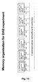
- 230000008520 organization Effects 0.000 description 15
- 230000001934 delay Effects 0.000 description 13
- 238000004364 calculation method Methods 0.000 description 9
- 230000008859 change Effects 0.000 description 9
- 239000000872 buffer Substances 0.000 description 6
- 238000004422 calculation algorithm Methods 0.000 description 6
- 238000004891 communication Methods 0.000 description 6
- 230000007423 decrease Effects 0.000 description 6
- 230000002123 temporal effect Effects 0.000 description 6
- 230000015556 catabolic process Effects 0.000 description 5
- 230000001419 dependent effect Effects 0.000 description 5
- 230000001976 improved effect Effects 0.000 description 5
- 230000008901 benefit Effects 0.000 description 4
- 238000006731 degradation reaction Methods 0.000 description 4
- 239000011159 matrix material Substances 0.000 description 4
- 230000005540 biological transmission Effects 0.000 description 3
- 230000000875 corresponding effect Effects 0.000 description 3
- 238000009826 distribution Methods 0.000 description 3
- 230000006870 function Effects 0.000 description 3
- 230000003993 interaction Effects 0.000 description 3
- 230000000737 periodic effect Effects 0.000 description 3
- 238000012546 transfer Methods 0.000 description 3
- 239000002699 waste material Substances 0.000 description 3
- 230000001276 controlling effect Effects 0.000 description 2
- 238000012937 correction Methods 0.000 description 2
- 238000010586 diagram Methods 0.000 description 2
- 239000003989 dielectric material Substances 0.000 description 2
- 238000011156 evaluation Methods 0.000 description 2
- 230000007246 mechanism Effects 0.000 description 2
- 230000007334 memory performance Effects 0.000 description 2
- 239000000203 mixture Substances 0.000 description 2
- 238000012986 modification Methods 0.000 description 2
- 230000004048 modification Effects 0.000 description 2
- 230000009467 reduction Effects 0.000 description 2
- 230000002040 relaxant effect Effects 0.000 description 2
- 230000035945 sensitivity Effects 0.000 description 2
- 238000000926 separation method Methods 0.000 description 2
- 239000007787 solid Substances 0.000 description 2
- 238000003860 storage Methods 0.000 description 2
- 230000009897 systematic effect Effects 0.000 description 2
- 238000003324 Six Sigma (6σ) Methods 0.000 description 1
- 230000009471 action Effects 0.000 description 1
- 230000003213 activating effect Effects 0.000 description 1
- 238000000137 annealing Methods 0.000 description 1
- 230000009286 beneficial effect Effects 0.000 description 1
- 239000000969 carrier Substances 0.000 description 1
- 230000001143 conditioned effect Effects 0.000 description 1
- 238000010276 construction Methods 0.000 description 1
- 230000002596 correlated effect Effects 0.000 description 1
- 239000013078 crystal Substances 0.000 description 1
- 230000009849 deactivation Effects 0.000 description 1
- 238000012938 design process Methods 0.000 description 1
- 238000001514 detection method Methods 0.000 description 1
- 238000010893 electron trap Methods 0.000 description 1
- 238000002474 experimental method Methods 0.000 description 1
- 239000002784 hot electron Substances 0.000 description 1
- 230000007257 malfunction Effects 0.000 description 1
- 239000000463 material Substances 0.000 description 1
- 238000005457 optimization Methods 0.000 description 1
- 230000003071 parasitic effect Effects 0.000 description 1
- 230000000135 prohibitive effect Effects 0.000 description 1
- 230000035484 reaction time Effects 0.000 description 1
- 230000004044 response Effects 0.000 description 1
- 230000000630 rising effect Effects 0.000 description 1
- 239000004065 semiconductor Substances 0.000 description 1
- 238000001228 spectrum Methods 0.000 description 1
- 235000013599 spices Nutrition 0.000 description 1
- 230000003068 static effect Effects 0.000 description 1
- 238000005309 stochastic process Methods 0.000 description 1
- 230000008685 targeting Effects 0.000 description 1
- 230000029305 taxis Effects 0.000 description 1
- 230000002277 temperature effect Effects 0.000 description 1
- 230000001052 transient effect Effects 0.000 description 1
- 238000010200 validation analysis Methods 0.000 description 1
- 235000012431 wafers Nutrition 0.000 description 1
Images


Classifications
-
- G—PHYSICS
- G11—INFORMATION STORAGE
- G11C—STATIC STORES
- G11C29/00—Checking stores for correct operation ; Subsequent repair; Testing stores during standby or offline operation
- G11C29/02—Detection or location of defective auxiliary circuits, e.g. defective refresh counters
- G11C29/028—Detection or location of defective auxiliary circuits, e.g. defective refresh counters with adaption or trimming of parameters
-
- G—PHYSICS
- G06—COMPUTING; CALCULATING OR COUNTING
- G06F—ELECTRIC DIGITAL DATA PROCESSING
- G06F30/00—Computer-aided design [CAD]
- G06F30/20—Design optimisation, verification or simulation
-
- G—PHYSICS
- G06—COMPUTING; CALCULATING OR COUNTING
- G06F—ELECTRIC DIGITAL DATA PROCESSING
- G06F30/00—Computer-aided design [CAD]
- G06F30/30—Circuit design
-
- G—PHYSICS
- G11—INFORMATION STORAGE
- G11C—STATIC STORES
- G11C29/00—Checking stores for correct operation ; Subsequent repair; Testing stores during standby or offline operation
- G11C29/02—Detection or location of defective auxiliary circuits, e.g. defective refresh counters
-
- G—PHYSICS
- G11—INFORMATION STORAGE
- G11C—STATIC STORES
- G11C29/00—Checking stores for correct operation ; Subsequent repair; Testing stores during standby or offline operation
- G11C29/04—Detection or location of defective memory elements, e.g. cell constructio details, timing of test signals
- G11C29/08—Functional testing, e.g. testing during refresh, power-on self testing [POST] or distributed testing
- G11C29/12—Built-in arrangements for testing, e.g. built-in self testing [BIST] or interconnection details
- G11C29/14—Implementation of control logic, e.g. test mode decoders
- G11C29/16—Implementation of control logic, e.g. test mode decoders using microprogrammed units, e.g. state machines
-
- G—PHYSICS
- G11—INFORMATION STORAGE
- G11C—STATIC STORES
- G11C29/00—Checking stores for correct operation ; Subsequent repair; Testing stores during standby or offline operation
- G11C29/04—Detection or location of defective memory elements, e.g. cell constructio details, timing of test signals
- G11C29/50—Marginal testing, e.g. race, voltage or current testing
- G11C29/50012—Marginal testing, e.g. race, voltage or current testing of timing
-
- G—PHYSICS
- G06—COMPUTING; CALCULATING OR COUNTING
- G06F—ELECTRIC DIGITAL DATA PROCESSING
- G06F2111/00—Details relating to CAD techniques
- G06F2111/06—Multi-objective optimisation, e.g. Pareto optimisation using simulated annealing [SA], ant colony algorithms or genetic algorithms [GA]
Definitions
- the invention relates to design methodologies for electrical systems, more in particular electrical circuits (especially digital circuits), to circuitry designed with said methodologies and to circuit parts, specially designed and incorporated within said digital circuits to enable operation of said circuits in accordance with the proposed concepts.
- DSM deep submicron
- IC integrated circuit
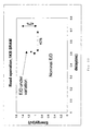
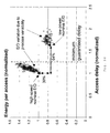
- Memories are among the most variability sensitive components of a system. The reason is that most of the transistors in a memory are minimum-sized and are thus more prone to variability. Additionally some parts of the memories are analog blocks, whose operation and timing can be severely degraded by variability, as illustrated in Fig. 1, showing the impact of process variability on the energy/delay characteristics of a 1 kByte memory at the 65 nm technology node.
- the solid blocks on the bottom left indicate the simulated nominal performance assuming no process variability (squares for writing and triangles for reading).
- the other points are simulation results incorporating the impact of variability (+-signs for writing and x-signs for reading).
- the energy consumption and delay of a memory designed using corner-point analysis is also shown (black circle).
- memories In a target domain of multimedia applications, memories occupy the majority of the chip area even in current designs and contribute to the majority of the digital chip energy consumption. Therefore they are considered to be very important blocks for a system.
- An object of the present invention is to provide improved design environments and methodologies for electrical systems, more in to provide particular improved electrical circuits (especially digital circuits, analog circuits ar mixtures or hybrids thereof), to provide improved circuitry designed with said methodologies or using said environments and to provide improved circuit parts, e.g. specially designed and incorporated within said electrical circuits to enable operation of said circuits in accordance with the proposed concepts.
- An advantage of the present invention is that it can avoid a worst-case design-time characterisation of circuits when designing electrical circuits taking into account the variability in IC parameters in deep submicron technologies.
- the present invention is based on the so-called design-time run-time separation approach, wherein the design problem is dealt with at design-time but some decision-taking is done at run-time, the design time part being adapted so as to generate a substantial freedom for a run-time controller.
- the worst-case design margins are alleviated by designing the circuit in a way that allows the unpredictability of its behaviour, even though the parametric specifications are not met at module level. For example, process variations in the manufacture of the actual circuit can be the cause of an unpredictable behaviour at run time
- the information provided by the design-time part is communicated to the run-time controller via a format, such as e.g. a table, wherein circuit performance parameters (like energy consumption, timing performance, quality of the operation) are linked to cost parameters, the performance-cost pairs together forming working points, said working points being pre-selected from a larger possibility set, said pre-selection being done at design-time.
- a format such as e.g. a table
- circuit performance parameters like energy consumption, timing performance, quality of the operation
- cost parameters like energy consumption, timing performance, quality of the operation
- the performance-cost pairs together forming working points
- said working points being pre-selected from a larger possibility set, said pre-selection being done at design-time.
- Pareto curves may be used for defining the pre-selected working points.
- working points within an offset of such a Pareto curve are used (so-called fat Pareto curve approach).
- these trade-off points for the criteria are not calibrated to the actually processed chip or the actual run-time conditions (such as temperature or process degradation). This calibration will occur with the actual circuit.
- the trade-offs can be and are preferably selected to be particularly useful with actual circuits, i.e. the trade-offs take into account typical process variations.
- the invention also includes a program storage device, readable by a machine, tangibly embodying a program of instructions, comprising: selecting working points for at least two tasks from actual measured Pareto-like information.
- a second aspect underlying the entire approach is the strict separation of functional and performance/cost issues, e.g. timing/cost issues.
- the functional correctness is checked by a layered approach of built-in self-test controllers, as described in conventional BIST literature, which check the correct operation (based on test vectors) of the modules.
- BIST is the technological approach of building tester models onto the integrated circuit so that it can test itself.
- Checking of the correct operation has to be based on a good knowledge of the cell circuits and DSM technology effects that influence the choice of the test vectors.
- system-level functionality checks may be needed to check that the entire application is working correctly on a given platform. Main system validation should happen at design-time, but if some of the DSM effects influence the way the critical controllers work, then these are better checked once at start-up time to see whether they function correctly.
- the present aspect of the present invention can be formulated as follows:
- a method for operating a terminal having a plurality of resources (modules) and executing at least one application in real-time, wherein the execution of said application requires execution of at least two tasks comprising selecting a task operating point from a predetermined set of optimal operating points, said terminal being designed to have a plurality of such optimal operating points, said predetermined set of operating points being determined by performing measurements on said terminal.
- DAB digital audio broadcast
- the invention will be illustrated for memory modules, in particular SRAMs (static random access memories).
- the present invention provides a method for generating a real-time controller for an electronic system, said electronic system comprising a real-time controller and an electronic circuit, the method comprising:
- the present invention also provides a run-time controller for controlling an electronic circuit, the controller comprising:
- the present invention also provides an electronic system comprising:
- the present invention also provides a method for generating a run-time controller of an electronic system, comprising an electronic circuit comprising a plurality of modules, and said run-time controller, the method comprising:
- the present invention provides a method for designing an electronic system, comprising a real-time controller and an electronic circuit, comprising of modules, the method comprising:
- the present invention provides a method for operating an electronic circuit, the method comprising:
- the present invention also provides a machine-readable program storage device embodying a program of instructions for execution on a processing engine, the program of instructions defining a real-time controller for an electronic system, said electronic system comprising a real-time controller and an electronic circuit, the program instructions implementing:
- a device A coupled to a device B should not be limited to devices or systems wherein an output of device A is directly connected to an input of device B. It means that there exists a path between an output of A and an input of B which may be a path including other devices or means.
- the invention may exploit, in one aspect, the system-wide design-time/run-time (meta) Pareto approach as described in US 2002/0099756 (task concurrency management), US 2003/0085888 (quality-energy-timing Pareto approach), EP 03447082 (system-level interconnect).
- the invention may exploit another trade-off approach.
- the approach of the present invention is to explicitly exploit a variation in system-level mapping to increase the overall cost/performance efficiency of a system.
- a difference between the method of the present invention compared to existing approaches is that the existing prior art methods try to monitor the situation and then "calibrate” a specific parameter. But in the end only one "working point” or “operating point” is present in the implementation for a given functionality. So no “control knobs” (control switches or functions) are present to select different mappings at run-time for a given application over a large set of heterogeneous components. The mapping is fixed fully at design-time. Moreover, the functional and performance requirements are both used to select the "working" designs/chips from the faulty ones. So these two key requirements are not clearly separated in terms of the test process.
- Fig. 2 An example is shown in Fig. 2 where there are originally two active entities (or tasks in this case), task 1 and task 2. Each of them has a trade-off curve, e.g. Pareto curve, showing the relationship between performance, in the example given task execution time, and cost, in the example given task energy.
- a trade-off curve e.g. Pareto curve
- a working point has been selected for the corresponding task, so that both tasks together meet a global performance constraint, in the example given a maximum "time limit" on the application execution time for the target platform (top right).
- the working point, e.g. Pareto point, for each task has been selected such that the overall cost, in the example given application energy, is minimized.
- a large performance range e.g. a large timing range
- the trade-off curve e.g. Pareto curve (as illustrated in Fig. 5, where performance/cost ratio is exemplified by access time/energy consumption ratio).
- Such large performance range can be achieved by a proper exploration/design/analysis phase at design time.
- This range will allow, according to the present invention, to compensate at run-time any performance uncertainties or variations, in the example given timing uncertainties or variations (whether they are spatial or temporal does not matter) as long as they are smaller than half the available range.
- this approach does not only deal with performance uncertainties due to process technology variations but also due to higher-level variations, e.g. due to a circuit malfunction (which changes performance, e.g. timing, but not the correct operation) or even architecture/module level errors (e.g. an interrupt handler that does not react fast enough within the system requirements).
- a circuit malfunction which changes performance, e.g. timing, but not the correct operation
- architecture/module level errors e.g. an interrupt handler that does not react fast enough within the system requirements.
- the working range on the performance axis has enough points available to compensate for the lack of performance, e.g. "lack of speed", compared to the nominal point, these variations can be compensated for at run-time.
- a nominal trade-off curve e.g. a nominal Pareto curve
- the nominal trade-off curve e.g. Pareto curve
- the nominal trade-off curve can be stored, e.g. in a Pareto point list stored in a table.
- an actual trade-off curve e.g. Pareto curve
- Pareto curve can be established, which may differ from the nominal trade-off curve due to process variations.
- any uncertainty in the actual timing of the circuit after processing can be compensated by shifting to another point on the "actual" trade-off curve, e.g. Pareto curve.
- the range for compensation equals the performance range, e.g. the entire time range, of the actual trade-off curve that can be designed such that it is larger than any of the potential uncertainties after processing.
- the position of the new working points i.e. the points on the actual trade-off curve
- the original points on the nominal trade-off curve could move to a non-optimal, e.g. non-Pareto optimal, position after processing. In that case, they are removed from the nominal trade-off curve as stored, e.g. the Pareto point list stored in tables.
- the original trade-off curve is preferably provided with an offset e.g. a so-called "fat" Pareto curve is established, which means that additional working points are added to the module that are initially above the trade-off curve, e.g. Pareto curve, but that have a high sensitivity (in the "beneficial direction") to parameters that are affected by processing. So these working points are likely to move to a more optimal position after processing.
- the best suited number and position of additional points in the trade-off curve with an offset, e.g. fat Pareto curve can be decided at design-time by analysis of a well-matched process variation model.
- substantially no slack or even no slack at all has to be provided any more in the tolerances for the nominal design on the restricting criteria (e.g. data rate or latency), and hence the likelihood of a significant performance and/or cost gain is high with the approach according to the present invention.
- the performance is still as good as the conventional approach can provide. This is based on the "robustness" of a run-time trade-off controller, e.g. Pareto controller (see below), to modifying the position of the trade-off curves, e.g. Pareto curves, even at run-time.
- a run-time trade-off controller e.g. Pareto controller (see below)
- the approach according to embodiments of the present invention involves a significant generalisation of the current "run-time monitoring” approaches, transposed in a digital system design context, where the monitored information is used to influence the actual settings of the system mapping. Furthermore, also a practically realisable implementation is proposed of the necessary “timing compensation” that is needed in such a system-level feedback loop.
- the operation of a system is divided into three phases, namely a measurement phase, a calibration phase and a normal operation phase.
- a measurement phase the characteristics of the circuit, e.g. all memories, are measured.
- a calibration phase a process variation controller (PVC) selects the appropriate configuration-knobs for the circuit, and applies them directly to the circuit.
- PVC process variation controller
- the phase of normal operation is for executing the target application on the platform.
- the cost is measured in function of performance of the circuit.
- each memory in the memory organization may be accessed a pre-determined number of times, e.g. four times, to measure read and write performance of a slow and a fast configuration. All these performance values for delay and energy consumption of a memory need to be updated in the PVC for each memory in the system. Furthermore for all of these pre-determined number of measurements (e.g. slow read; slow write; fast read; fast write) the worst-case access delay and energy of each memory needs to be extracted.
- a methodology for doing this has been proposed in H. Wang, M. Miranda, W. Dehaene, F. Catthoor, K.
- test vectors are generated based on two vector transitions that can excite the memory addresses which exhibit the worst-case access delay and energy consumptions. These test vectors are generated in a BIST-like manner. Furthermore a memory has also different delays and energy consumptions for each of its bit- and wordlines. Therefore the worst-case access delay and energy consumption have to be calculated. This calculation is done already within monitors or monitoring means (see below) and so only the worst-case values have to be communicated over the network.
- the process variation controller reads a first test vector from a test vector memory and configures the network in order to be able to communicate with the memory under test. Also delay and energy monitors are connected to the memory which is currently under test. The functional units of the application itself are decoupled from this procedure. Then the PVC applies a test vector including address and data to the memory. In a first step the memory is written and so the ready bus of the memory is connected to the delay monitor. The time to apply one test vector to the memory is equal to one clock-cycle. For measurement the clock is configured via a phase-locked-loop in a way that the monitors have a stable result before the beginning of the next clock-cycle.
- the memory In the next clock-cycle the memory is read from the same address as before, so the same test vector is still in use. In this cycle the data-out bus of the memory is connected to the delay monitor in order to measure the time after which the output of the memory is stable. In a third step the memory configuration-knob is changed from slow to fast which means that the memory is now configured to its faster and more energy consuming option. Still the same test vector is applied and step one and two are repeated for the fast configuration-knob of the memory under test. These four steps which are described in Fig. 6 are repeated for all test vectors of the memory under test.
- the delay and energy monitors send back the maximum delays and energy consumptions of all pre-determined, e.g. four, possible options of this particular memory under test.
- the pre-determined number e.g. four, maximum delay and maximum energy consumption values (e.g. each for slow read, slow write, fast read and fast write) are stored into a register file within the PVC in order to be able to decide during the calibration phase which configuration of the memory has to be chosen.
- the PVC tells the system-level-controller that the measurement phase is finished.
- the system-level-controller is now the one which has to decide how to proceed. Usually it decides now to proceed with the calibration phase, in which the most efficient memory configuration for the system has to be found.
- the PVC configures the memories of the system in order to meet the actual timing requirements of the application. Therefore the PVC uses dedicated control lines which are connected to each memory of the architecture.
- the PVC Apart from the information about delay and energy of each memory, which information was stored during the measurement phase, the PVC holds information about the current timing constraint for the specific application.
- This timing constraint is also stored in a register and can be changed at runtime, if the register is memory-mapped. The timing constraint is generated during the design-time analysis of the application according to the bandwidth requirements of the application.
- the PVC is calculating all necessary information to configure the configuration-knobs of the memories in order to meet the timing constraint. These calculations are depending on the adaptation the controller operates on. In clock-cycle-level adaptation the controller will only decide based on the configuration-knobs the memories are providing. In time-frame-level adaptation the controller is providing more accurate configurations gained from the fact that the application is time-frame based and the functional units are executed sequentially. Based on the information gained with one of the two approaches the most efficient configuration for the memory configuration-knobs in terms of delay and energy is applied.
- Normal operation is the phase where the target application is executed on the functional units of the platform. All other components like the PVC and the energy and delay monitors are virtually hidden by an appropriate configuration of the communication network. During this phase the memory management unit of the functional units takes care of supplying the source and destination block information to the network.
- this memory management unit of the functional unit was implemented within the system-level-controller.
- the functional units themsalves were abstracted away by simulating their I/O behavior. So the functional units itself are implemented as a Finite State Machine which communicates in a cycle-accurate behavior with the memories.
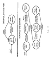
- the memory accesses in normal operation mode are simulated by the three different Finite State Machines which are representing the FFT, the Deinterleaver and the Viterbi of the application driver.
- Fig. 8 shows the different memories and their corresponding functional unit. The memory accesses were simulated by using this scheme.
- the monitors and the stored C-R-Q values in the trade-off surfaces do not have to be extremely accurate because the trade-off run-time controllers, e.g. Pareto run-time controllers, are quite "robust" to (small to medium) errors.
- the trade-off run-time controllers e.g. Pareto run-time controllers
- the trade-off control manager e.g. Pareto control manager
- can relax the trade-off working point e.g.
- Fig. 9 describes the design-time phase, generating so-called design trade-off information, e.g. Pareto information.
- Fig. 10 describes the calibration phase, determining so-called actual trade-off information, e.g. actual Pareto information, and the run-time phase, exploiting said actual trade-off, e.g. Pareto, information.
- the addition of the calibration phase is known in previous design-time run-time Pareto approaches..
- the deactivation of failing circuitry within the design digital system is an additional feature.
- the vendor will not have full control on the mapping environment that designers use for their applications. In that case, it is not possible to incorporate the design-time exploration phase (which is application-specific) in the design/tool flow.
- mapping environment or the designer himself will then still perform a specific assignment of the data to the circuit, e.g. memories. It is assumed that this assignment is expressed to a tool that converts this to a table that is stored in the program memory organisation of the embedded processor that executes the run-time trade-off, e.g. Pareto, controller dealing with the process variation handling.
- This run-time trade-off controller e.g. Pareto controller
- the invented approach splits the functional (which modules works) and performance/cost aspects of a part or the entire application mapping/platform design process.
- the invention will work properly if the trade-off, e.g. Pareto, hyper-surface retains the same shape from the design-time simulation to the physical processed one (which can partly be included as a design criterium). If the change is too large, the use of a trade-off curve with offset, e.g. a so-called "fat Pareto curve", (incorporating non-optimal working points in the design trade-off curve lying within a predetermined offset of the optimal points) can be used to compensate for small shape changes.
- a trade-off curve with offset e.g. a so-called “fat Pareto curve”
- Memory matrices are complicated circuits, containing analog and digital parts.
- the decoder consumes a significant part (over 50%) of the delay and energy.
- the bitlines consume potentially much more than the sense ampliflier (SA) because the SA is only active for e.g. 32 bits, whereas the bitlines span 128 bits (even in a divided bitline memory the bitlines span more than 1 word). Both components will now be analysed.
- SA sense ampliflier
- process variation always degrades delay, because many parallel outputs exist and the decoder delay is the maximum of all the outputs.
- the "nominal" design is the fastest because all paths have been optimised to have the same "nominal" delay.
- the analog parts of the memory are also heavily affected by process variation.
- the delay is normally increased because several bitlines are read/write in parallel to compose a memory word. If, due to variations, the driving capability of one of these cells decreases, then during the read operation the swing in voltage in the affected bit-line will be less in magnitude than in the nominal case. In this case the sense amplifier will require more time to "read" the logic value than nominally. Indeed, it would be necessary to have all active cells in the selected word to have a higher driving capability than the nominal one and that one to be larger than the delay occurring in the decoder so as to have a memory operation faster under variation than in nominal operation.
- the total system energy is the sum of the memories' energy weighted by the number of accesses to each of them. Preferably this should be separate for the reads and writes because they have different behaviour (see Fig. 13 + Fig. 14).
- the system delay is the worst case delay of all the memories that are active, since all memories should be able to respond in one clock cycle. If process variation cannot be compensated for at run-time, a worst-case is to be assumed at the design-time characterisation. Obviously not all extreme delay values can be counteracted, so typically a 3 sigma range is identified. This will determine a yield value after fabrication during the test phase, because all the points beyond 3 sigma range will be invalid.
- a mechanism is provided to recover the excessive delay that is introduced by solving the problem at the "clock cycle" level.
- a compensation for the effects of process variation is performed in the system level timing. For multi-media systems which are stream based this means for instance that it has to be guaranteed that every frame the outputs are computed within the given timing requirements. E.g. for the DAB 12M cycles are available per audio frame. If, at some frame, one or more memories go above the original (design-time) delay specification (which is now not selected worst-case any more), according to the present invention it should be possible to speed up the memories at run-time.
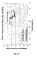
- Pareto optimal mappings is at design-time already stored in the program memory (in a compressed effective form). This leads to several trade-off, e.g. Pareto, curves that depend on the exact point that is active in the process variation "cloud” and that are quite different in position compared to the worst-case (3-sigma) curves (see Fig. 17).
- the run-time controller that has to start up a new frame, first selects the appropriate cost/performance trade-off point, e.g. energy-delay Pareto point, and loads the corresponding program in the L1-I cache. In the worst case this has to change every frame (which is still only every 12Mcycles for a 24ms frame and 500MHz clock for the DAB) but usually the same point will be valid for several frames even because usually the temperature effects will not cause that fast changes. So the L1-I loading is negligible in both energy and performance effect.
- the appropriate cost/performance trade-off point e.g. energy-delay Pareto point
- a calibration step may be added after the chip fabrication by using an on-chip calibration loop (see Fig. 18) and probably also once-and-a-while during the life-time of the chip because several effects like degradation will influence the actual cost/ performance, e.g. energy-delay, positions of the trade-off optimal mappings, e.g. Pareto-optimal mappings.
- the same (few) test vectors that are used at design-time to determine the delay and energy of a memory are used at calibration time to measure these values with monitors.
- Delay can be monitored with delay lines that have been up-front calibrated from e.g. a crystal and that are designed with wide transistors so that the delay lines are not influenced much by further variations.
- the energy monitor is based on current measurement, also with wide transistor circuits.
- the calibration should be done separately for read and write operations.
- DSM Deep Sub-Micron
- Process variation impacts many technology parameters. The focus here is on those related to the transistors, the effect of variability in the interconnect wires is neglected here since its impact in the back-end processing is expected to be less dramatic than in the front-end. This is true for the long interconnect lines such as bit-lines, word-lines or decoder busses that are typically large enough so as to average variability effects. Impact of variability at transistor level can be reflected in deviations in the drain current. This deviation can be modeled using the threshold voltage (Vt) and the current factor (Beta), which depends on several physical parameters (Cox, mu, W/L). A first order analysis shows that the variabilities of these two electrical parameters are dependent on transistor area.
- Vt threshold voltage
- Beta current factor
- sigmaVt DeltaVt/sqrt(WL)
- sigmaBeta DeltaBeta/sqrt(WL) where W,L are the width and length of the transistor.
- Beta can only be modeled in HSPICE via physical parameters.
- the oxide capacitance (Cox) and mobility (mu) cannot be modified since they are correlated with other transistor parameters like gate capacitance. Therefore variability in Beta must be modeled implicitly. Since Beta is proportional to the aspect ratio of the transistor W/L it has been chosen to model that variability as changes in W/L such that WL is constant. This ensures that the first order contribution of the extrinsic load driven by the transistor is not influenced by the variation in Beta, which is in fact physically the case.
- the SRAM architecture considered for analysis is the cell-array partitioned architecture typically used in industry, and described in B. Prince Semiconductor Memories: A handbook of design, manufacture, and application, second edition John Wiley and Sons, 1991.
- the row decoder is split in two stages, with a predecoder stage composed of NAND gates and a postdecoder stage composed of NOR gates
- the cell-array is composed out of parallel bitlines and wordlines with the cells (classical 6T SRAM cell design) dimensioned to perform stable operations at the 65 nm technology node.
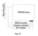
- the timing control interfaces uses a self-timed style described in by Steve Furber in "Asynchronous design for tolerance to timing variability", ISSCC04 Advanced Solid State Circuits Forum, generating not only a short pulse for the wordline but also other control signals according to the row decoder output (see Fig. 19).
- the precharge circuit, column mux and write circuit in the array are also optimized for the technology node and SRAM size.
- the (voltage) Sense Amplifiers (SA) and tri-state output buffers used are designed for the 65nm node as well.
- HSPICE simulations of the full SRAM is not practical for analysis of the process impact due to the many simulations required to gather data with reasonable statistical significance. Therefore, for the purpose of speeding up simulation time without sacrifying much accuracy, a lumped SRAM model (see Fig. 20) targeting less simulation time and with still reasonable accuracy is developed for this analysis.
- This model is composed out of a full row decoder plus a simplified cell-array where the number of wordlines is just a fraction of the ones present in the full memory and they are equally distributed along the height of the cell-array. Still, it should be mentioned though that results with from HSPICE indicate that this lumped model achieves more than 97% accuracy in average with a factor of 12 reduction in the simulation time compared to the full SRAM simulation.
- the critical path of the SRAM starts from the row decoder and ends at the output buffer in the array.
- the delay of this path under process variations can be obtained in the netlist by connecting the row decoder critical path with the array and finding the delay of the slowest output out of all parallel outputs of the array.
- the first issue in this step is to find the worst case decoder delay (hence the critical path) under process variability.
- This is not a trivial task as the decoder critical path depends not only on the input address but also on the transition from the previous address. This is becasue such transition changes the (dis)charge paths of the parasitic capacitances of the decoder netlist, and hence affects the actual delay.
- a worst case transition exists for a netlist not subject to variability and that is always the same. However, under variability that is not necessarily the case. The reason is that many parallel decoding paths exist in the combinational decoder. Hence, the slowest path that determines the row decoder delay is different depending on the variability. Finding this critical path or slowest output actually means finding a worst case delay transition that excites this output for each netlist injected with a different variability set.
- Step2 to obtain the worst delay vector in step2, exercising all decoder outputs one by one is not a time efficient solution since the number of combinations grow as 2 over n, n being the number of address decoder inputs.
- a heuristic has been developed which is based on exciting all decoder output at the same time and finding the slowest of them. This is done by violating the decoding rule in such a way that all input address bits and their complemented bits (see Fig. 21) are supplied with the same 0-1 transition at the same time no matter a particular input should be complemented or not.
- the all-1 vector will be used to excite all the decoding paths in the decoder that will allow activating all the outputs in one time without wasting time by trying it one by one.
- the slowest one can be easily identified. Based on this output, the worst delay vector can be obtained by backtracking the decoding process. Input address transition will not play a role in the determination of this vector because the same transition (0-1) is applied for all the outputs.
- the worst case delay transition set under process variation can be obtained by generating a set of 2 input address vectors.
- the first vector of that set is the initial vector exercising a worst case transition (of the possible set of all possible worst case transitions) irrespective of the decoded output (see Step1). That one is then followed by the vector selecting the worst case output (see Step2).
- the worst decoder transition is obtained by applying two vectors, where the second vector is the same as for delay. Only the first vector is different, still obtained by complementing the first of the vectors for worst case delay. That should lead to opposite switching direction in the nodes of the netlist while creating maximum activity in these nodes.
- the delay of the SRAM is obtained as follows: (1) a nominal lumped netlist of the memory is first instantiated; (2) random variations on the transistors of that netlist are injected generating a netlist for a given variability; (3) the decoder of that netlist is analysed and the worst case delay and energy transitions are found following the methodology described before; (4) once the decoder output with the worst case delay for a given variability scenario is identified, then a new netlist is generated by connecting that (slowest) output with the one of the four wordlines of the lumped cell-array netlist; (5) the write delay is measured from the moment the input address is given to the moment when the last cell in the accessed bitlines becomes stable; (6) the read delay is measured from the time the address is given to the time when the slowest data bit is read out among the all the parallel bitlines.
- Fig. 21 The experimental results shown in Fig. 21 indicate that decoders under process variation tend to have larger delay and energy than the nominal one.
- the increase in decoder delay is because the slowest path of the decoder under variability will be slower than the one in the nominal decoder for most cases.
- the energy increase is due to the fact that reconvergent decoding paths have different delays induced by process variation. This difference in delay leads to glitches when they converge at one gate. This wasted energy leads to the increase in overall decoder energy.
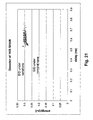
- the delay/energy cloud of the memory for read and write operation are shown in Fig. 22 and Fig. 23 respectively.
- the delay of both operations tends to become slower in most cases.
- This increase in delay not only comes from longer decoder delay but also from the larger array delay.
- the array tends to have larger delay because in most cases the slowest bitline among the parallel ones being read is slower than nominal case.
- the increase in delay is due to the fact that sense amplifiers need more time to sense the smaller-than-nominal voltage swings on this particular bitline to full rail. This smaller swing is due to several effects, even a combination between them. For instance, the bitline discharge current can be reduced due to the pass transistors conducting later than nominally (due to a higher Vth than nominal).
- the inverters in the cell can have less driving capability due to the impact of variability in Vth.
- the read delay is for most cases larger than nominal.
- the energy of the read operation is dominated by the energy consumed on the bitlines including both the active ones (these being selected by the column muxes) and the passive ones (these not selected).
- bitlines have larger swing than nominal, they consume also more energy than in the nominal case to discharge the bitline load.
- bitlines have less voltage swing, they also consume less energy.
- the higher read energy in the cloud is due to the fact that most bitlines under that variation have larger voltage swing making the overall energy contribution to increase.
- delay has the same trend as in the read operation for similar reasons. For instance, one end of the cell is directly grounded by a large transistor in a very short time. While the other end of the cell has to be flipped by one of the inverters in the cell. Affected by variability, that inverter in the slowest bitline has less driving capability than nominal case, which results in the cell taking more time to get totally flipped. All bitlines would be required to react faster than the nominal bitline and that gain in delay woud be required to become larger than the excess in the decoder so as to have an overall memory with a faster reaction time than the nominal memory. That is in fact extremely unlikely to happen as simulation results confirm.
- An architecture for monitoring a circuit is provided.
- a developed architecture for an experimental setup with a DAB receiver is described in detail.
- Fig. 25 the final architecture of the system including the simulated functional units of the DAB receiver is shown.
- it is not intended to limit the present invention to this particular architecture. From the description of the architecture below, a person skilled in the art will be able to build other architectures for other circuits.
- the architecture of the system including the simulated functional units of the DAB receiver includes the nine memories which are required by the DAB receiver. To provide the DAB receiver with a parallelism of three parallel data transfers the memories are grouped into memory domains and each domain is assigned different address and data busses. These three pairs of busses have their own delay monitor to avoid inaccuracies due to different wire lengths of the busses. Via the input/output-ports of the system the simulated functional units are connected to the busses.
- an energy monitor To measure the energy consumption of an access to a memory, an energy monitor is needed.
- the energy monitor is connected to the power supply of each memory. Potentially one energy monitor per memory might be required for more accuracy in the measurement results. It also needs information about when to start and when to stop the measurement in order to provide sufficient results.
- Only a simulation of an energy monitor is implemented in the VHDL description of the system, because energy related behavior cannot be simulated in VHDL. Therefore just a register file which contains information about all the different energy consumptions per access of each memory is read by the monitor. To synchronize the monitor with the current memory under test in order to get the correct energy values out of the register file a synchronization with the clock of the system is necessary.
- the different maximum energy values for read and write for the slow and fast configuration-knob are stored in registers. After the measurement of one memory is completed the content of these registers is sent to the process variation controller (PVC). After the measurement of all memories in the design the PVC has information about all possible configurations in terms of energy for the complete memory architecture.
- the energy values are sent to the PVC via a dedicated bus. This could be optimized in future by sending the values over the data bus which is not in use during the time the values are sent back and which is connected to the monitor anyhow.
- the monitor itself consists of two separate chains of delay lines and it measures the time difference between the rising edge of two different signals.
- the first signal, called start signal is sent through a slower delay line chain and the second signal, called test signal through a faster delay line chain in order to catch up with the start signal.
- Comparators are introduced along these chains. When the test signal catches up with the start signal the respective comparator output becomes true. So the output of the delay monitor is a so called thermometer code gained from all single comparator results.
- the time difference between the two edges is then calculated as the number of delay line times the delay difference between delay lines of the fast and the slow chain.
- This delay monitor can measure the delay difference between two one-bit signals. So the granularity of the measurement is defined by the delay difference between the fast and slow chain.
- the delay of the stages of the fast line is 50 psec, for the stages of the slow line it is 100 psec. Therefore the accuracy of this circuit is 50 psec which is sufficient given the performance of current embedded memories.
- One stage of the delay line chain consists of buffers in each line which introduce the delay and a comparator. To be able to measure a range of delay from 400 psec up to 1.55 nsec 23 delay line stages have to be used. Additionally an initial delay of 400 psec exists before the delay line chains in order to save stages. This is feasible due to the fact that no delay lower than 400 psec has to be measured. The measurement results given in a thermometer code of a length of 23 bits is analyzed and transformed into a five-bit value.
- the complete delay monitor of the architecture consist of 32 such one-bit monitors and 32 registers of five bits each, as illustrated in Fig. 26.
- the 32 monitors asynchronously measure the delay of the different memory output bits and store them in a register.
- To calculate the worst-case delay of a single bitline all the measurement results of one bitline are written into a 32 times 5 bit registerfile.
- a unit, called the StoreMaxDelay, is provided for storing worst-case delays.
- the StoreMaxDelay-Unit is comparing in parallel the contents of the 5 bit registerfile and the worst-case delay is stored in a register.
- this register where the worst case delay is stored is only updated when another bitline delay is bigger than the stored worst-case delay.
- the number of registers where the worst-case delays are stored is equal to the predetermined number mentioned above, e.g. four when the maximum read and write delay for the slow and fast configuration-knob are measured. Similar to the energy monitor the four maximum delay values stored in these registers are sent to the PVC after the complete measurement of one memory.
- the PVC is responsible for the control of the measurement and calibration and configuration-knob selection of the memory architecture. It is implemented as a Finite State Machine for the measurement and calibration phase.
- the PVC can calibrate the memories to a given cycle-time constraint or to a given time-frame constraint. This functionality leads to two different implementations of the PVC which are discussed next.
- This version of the controller measures only the delay per access of the memories, since only delay adaptation can be achieved using this technique.
- the PVC is based on a system that has a fixed clock frequency in normal operation phase. So the memories of the system have to meet a fixed cycle-time constraint. This constraint is defined at design-time of the architecture and stored into a register which is known by the PVC.
- the PVC measures the maximum delay values for each configuration of the memory architecture (slow read; fast read; slow write; fast write) and stores them into a register file.
- the maximum delay of a memory per configuration-knob is calculated. To make sure that the slow configuration-knob of the memory is really slower than the fast one also these two maximum delays which were calculated before are compared. This problem could occur if the memory clouds overlap.
- the maximum delay of each memory is then compared to the cycle-time constraint. If the memory can meet the constraint with its less energy consuming slow configuration-knob there is no need to adapt. In case the memory cannot meet the constraint with this configuration-knob it has to be configured with the fast configuration-knob.
- SLC system level controller
- the time-frame-level implementation of the PVC additionally needs the energy consumption per access of each memory in the architecture. So the controller holds information about the maximum delays and energy consumptions per access of the complete memory architecture. Based on this information it is able to decide how the memories need to be configured in order to meet a given real-time constraint for executing the target application on the chip. This real-time constraint is obtained at design-time and stored into a register. Furthermore the PVC needs information about the number of cycles each functional unit uses within one time-frame. So this PVC can only be used for frame-based applications in which the functional units are executed sequentially. For the application of the DAB receiver this time-frame is one single audio-frame.
- the PVC splits the normal operation phase where the functional units are executed into three more phases (see Fig. 28): execution of the FFT, the Deinterleaver and the Viterbi.
- the clock of the system can be adjusted, more particularly its frequency can be adjusted.
- the configuration-knob of these memories has to be adjustable at the boundary of each phase or functional unit.
- the execution of the Viterbi is the most energy consuming and slowest phase in normal operation. It might be necessary that the clock of the system has to be slowed-down to make sure that all memories accessed during the Viterbi can be accessed within one clock-cycle in their slow and less energy consuming configuration-knob. In order to meet the time-frame constraint the memories of one or both of the other two phases might have to use the fast and more energy consuming configuration-knob. So with this configuration the PVC can allow the lowest possible energy consumption for executing one audio-frame of the DAB receiver and it still makes sure that the time-frame constraint can be met. Of course with the assumption that the system is properly designed.
- the first step the PVC does after the start-up of the system is again a measurement phase.
- the PVC is able to enter the calibration phase.
- the maximum delay of each memory for its slow and fast configuration-knob is calculated.
- the tightest cycle-time for low-power and high-speed configuration of each functional unit can be obtained.
- the memories of one of these three phases can only be switched to the same configuration knob.
- the energy consumption and the execution time for processing one audio-frame of the DAB receiver is calculated based on the measured information about the memory architecture.
- the access frequencies of the memories are needed. They are available in registers. So, as can be seen in Fig. 29, in the next step the energy consumption and the execution time for each configuration are calculated. The results for each configuration are stored into a register file. With all the calculated information a trade-off cost/ performance curve, e.g. a Pareto energy/execution time trade-off curve, can be obtained. Based on this trade-off curve the closest configuration to the time-frame constraint which has the lowest energy consumption is chosen. In the next step this configuration is applied to the memory architecture via the memory configuration-knobs.
- a trade-off cost/ performance curve e.g. a Pareto energy/execution time trade-off curve
- This controller is responsible for the execution of the different phases at the right time. So the SLC is implemented as a Finite State Machine that defines which phase is going to be executed. After the start-up of the system the SLC starts the measurement phase of the PVC. After the PVC has finished with the measurement phase a done signal is received by the SLC. So the SLC knows that measurement is done and starts the calibration phase of the PVC. After completing the calibration again a done signal is received and the SLC starts the normal operation phase in which it acts as the memory management unit of the functional units and provides the network controller with the right source and destination block-addresses. This memory management functionality within the SLC is also implemented as a Finite State Machine.
- the SLC also transmits and receives start and stop signals to and from the functional units. This is necessary because the SLC has to tell the PVC and the PLL at the boundary of each of the three phases in normal operation phase to switch the memory configuration-knobs and to adjust the clock frequency.
- the SLC can be replaced by an instruction-memory-hierarchy and the signals which are needed for synchronization issues can be removed.
- a controller will configure the memories at run-time to a setting which meets the cycle time constraints in case the real-time execution constraints are violated after fabrication.
- the memories of the architecture are implemented with a completely asynchronous interface.
- a package with timing information e.g. generated by a C-program, is involved in the VHDL description of the memory.
- the memory is provided with different delays for each bitline.
- the memory has a process which is listening to the address and data port.
- the process starts adding the delay of the memory due to process variation as described above.
- the process is creating an internal signal, and when this signal is stable too, the data is written into the memory or transfered to the output port depending on whether the memory is currently read or written.
- the memory also drives another output called ready port. This port is necessary to measure the write delay of a memory as discussed above.
- the three different address, data and ready buses shown in Fig. 25 are implemented in the communication network based on segmented buses.
- the memory organizations of low-power systems are typically distributed so a centralized switch implementation would be a bad design choice.
- This communication network provides a bandwidth of three parallel transfers per cycle.
- the buses are bi-directional shared connections among a number of blocks and the long wires are split into segments using switches.
- the SLC and the PVC have to supply a source and a destination block-address and the number of transactions which are performed in parallel.
- the PVC has to do this in the measurement phase when it is applying test vectors to the memories and reading the measured values from the monitors.
- the SLC takes care of applying the right block-addresses in normal operation phase instead of the memory management unit of the functional units as mentioned in the section about the system level controller.
- a small network controller with a look-up table controls the configurations of these switches. Based on the source and destination block-address of the current communication the controller finds the correct entry in the table and applies it to the switches.
- phase-locked-loop is the adaption of the system clock.
- the clock frequency is adapted at the boundaries between the functional units in normal operation phase.
- the clock is relaxed to a clock-cycle of 3 nsec to make sure to have stable results from the one-bit monitors (see above).
- This frequency divider is able to adjust the frequency of the system to a given value.
- This value is applied by the SLC for all different phases. In normal operation phase the SLC receives this values from the PVC.
- the approach of the present invention includes a minimal compile-time and a synthesis-time phase to accomplish run-time compensation of the impact of process variability and energy consumption minimization.
- compile-time the mapping of the application data into the available memories has been determined, and the timing constraint to achieve real-time operation of the system has been calculated. Based on this information also the number of cycles for the various parts of the application can be extracted as well as the number of memory accesses of each of these parts. The impact of variability is neglected in this stage.
- the architecture which includes a controller and run-time configurable memories is developed. This architecture is able to adjust itself to meet the application deadlines, by adjusting the memory configurations and the clock frequency to meet the application timing constraints.
- the memories available on the platform offer run-time reconfigurability, as illustrated in Fig. 30, showing transistor level simulations at 65nm, e.g. a low-power option and a high-speed option which can be switched at run-time.
- Process variability severely impacts the cost/performance, e.g. energy/delay behaviour of the memories.
- the actual energy/delay performance is a point in each cloud.
- One important property of these clouds is that they should not overlap in the delay axis. If this is satisfied then the actual high-speed memory performance is always faster than the actual low-power performance irrespective of the impact of variability on delay. This property is exploited by the run-time controller to guarantee parametric yield.
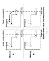
- Fig. 31 illustrates how the controller adapts the memory configurations to guarantee parametric yield.
- the energy/delay characteristics of two identical memories are shown. Their nominal behavior is the same, but after fabrication their actual performance differs due to process variability.
- memory A has to be switched to its high-speed and high energy consumption configuration to meet the global timing constraints, while memory B does not. Since the two clouds for the two configuration options of memory A do not overlap in the delay axis, it is guaranteed that this configuration will meet the timing constraints.
- parametric yield is guaranteed, as long as the application cycle time constraints do not become lower than the minimum guaranteed delay of the slowest memory.
- the technique according to the present invention includes a compile-time and a synthesis-time phase.
- compile-time the characteristics of the application are extracted, for example the number of cycles per functionality needed for decoding one audio frame, the mapping of application data to memories and the subsequent number of accesses per memory.
- the simplest way to use the fore-mentioned technique is to determine an optimal cycle time for the application and to let the memory organization adapt to this constraint.
- the computation of this constraint is straightforward after the application mapping (or RTL description) step, the real-time constraint for the execution time of the application divided by the number of cycles required to run the application yields the target cycle time.
- this cycle time should not be smaller than the minimum guaranteed delay that the platform can offer, see Fig. 30.
- the memories in the organization are adapted based on the basic principle described in the previous section. As shown in Fig. 32, the measurement, calibration and memory configuration steps are only executed once at the start-up of the system and then the application is run without any modifications.
- the technique described can only compensate for the impact of variability which does not vary temporally; it cannot compensate for the impact of the varying temperature on the performance of the memory organization.
- the only information needed is the number of cycles for executing the application, which is always defined in any implementation design flow.
- the target clock frequency is calculated from the real-time constraint of the application. At run-time the only required functionality is a comparison between the actual memory performance and the target clock frequency and potentially adjusting the memory configuration.
- a simple extension can allow this technique to compensate for the impact of process variability at a finer granularity, namely at the beginning of each frame.
- the measurement phase and the calibration phase can still be done only once at the start-up of the system. If the memory configuration step, however, is done at the beginning of each frame then also the impact of temperature and other temporally varying effects can be compensated.
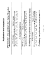
- a more complex way of compensating delay is to distribute the available execution time between the various application functionalities in such a way that the cycle time is not constant throughout the execution of the application. If it is assumed that the different functionalities of the application are performed in a serial way (one after the other as opposed to a parallel way as in a pipeline), then the clock cycle needs to change in a temporal way. For a few milliseconds it will be 10ns and then for another few milliseconds it can change to 20ns, for instance. If the functionalities are pipelined, thus executed in parallel, the cycle time needs to change in a temporal and in a spatial manner. This introduces side-effects in case memories exist that are used by more than one application functionality.
- Fig. 33 shows how the available execution time can be distributed among the various functionalities.
- a simple application is assumed which first performs an FFT operation on some input and then performs a Viterbi operation. These two operations are executed one after the other.
- the available execution time has to be distributed between the two functionalities in an optimal manner.
- the FFT functionality performs a first number of memory accesses per cycle, e.g. one, and that the Viterbi functionality performs a second number of parallel memory accesses per cycle, e.g. three.
- the FFT needs a first number of cycles to execute, e.g. 6, and the Viterbi needs a second number of cycles, e.g. seven; this can be easily generalized.
- the execution time is distributed evenly between the total of the first and the second number of cycles, in the example given between 13 cycles of the application, the memories need to be configured to the high-speed option.
- the memories can be configured to their low-energy option. This means that in the time distribution shown on top in Fig. 33 the memories need to be always configured at high-speed; in the middle case they are in the high-speed mode for the FFT and in low-energy for the viterbi and vice versa for the bottom distribution.
- E total NPA Viterbi ⁇ NC Viterbi ⁇ E memory ⁇ NPA FFT ⁇ NC FFT ⁇ E memory , where NPA x stands for number of parallel accesses for functionality X and NC x stands for number of cycles for functionality X.
- This method of compensating at the application level exploits the characteristics of the application.
- the number of available operating points is only dependent on the application and can be very high, because any realistic application can be split into many functionalities.
- the granularity of the results depends only on the application and even if the memory organization consists of a single memory, still a reasonable energy consumption - execution time range can be obtained for the entire application.
- introducing more operating points requires a more intensive calculation of the optimal operating points at the measurement and calibration phases. And even though, the execution time for these calculations is not an issue, since they are done only once, the complexity of the hardware blocks that performs them and its area may become significant.
- DAB Digital Audio Broadcast
- the transmission system in the DAB standard is based on an Orthogonal Frequency Division Multiplex (OFDM) transportation scheme using up to 1536 carriers (Mode I) for terrestrial broadcasting.
- OFDM Orthogonal Frequency Division Multiplex
- the OFDM carrier spectrum is reconstructed by doing a forward 2048-point FFT (Mode I) on the received OFDM symbol.
- This functionality is assigned to the FFT processor shown in Fig. 35.
- Forward error correction and interleaving in the transmission system greatly improve the reliability of the transmitted information by carefully adding redundant information that is used by the receiver to correct errors that occur in the transmission path.
- the frequency and time de-interleaver blocks unscramble the input symbols and the Viterbi processor is the one performing the error detection and correction based on the redundant information.
- the energy optimal mapping of the DAB application data results in a distributed data memory organization that consists of nine memories, seven of them having a capacity of 1 KByte, one of 2 KByte and the last one of 8 KByte. Their bitwidths are either 16 or 32 bits.
- Fig. 36 shows a simplified original Finite State Machine for the execution of the DAB application without the process variability compensation technique (top) and the one including it (bottom). Additional states are needed to accommodate for the measurement and calibration phases which are executed seldom as well as the state where the memories are configured. As mentioned earlier, these additional states required for the compensation can be added without affecting the control of the application execution.
- the controller calculates the optimal cycle times for execution of the FFT and de-interleavers and for the execution of the Viterbi, such that the real-time operation is guaranteed and global energy consumption is minimized.
- the knob selection phase is where the controller configures each memory to meet the required cycle time constraint.
Landscapes
- Engineering & Computer Science (AREA)
- Physics & Mathematics (AREA)
- Theoretical Computer Science (AREA)
- Computer Hardware Design (AREA)
- Evolutionary Computation (AREA)
- Geometry (AREA)
- General Engineering & Computer Science (AREA)
- General Physics & Mathematics (AREA)
- Design And Manufacture Of Integrated Circuits (AREA)
Priority Applications (1)
| Application Number | Priority Date | Filing Date | Title |
|---|---|---|---|
| EP05020770A EP1640886A1 (fr) | 2004-09-23 | 2005-09-23 | Méthode et appareil pour la conception et fabrication de circuits électroniques sujets à des problèmes de fuite à cause d'écarts de température et/ou de vieillissement |
Applications Claiming Priority (4)
| Application Number | Priority Date | Filing Date | Title |
|---|---|---|---|
| GBGB0407070.2A GB0407070D0 (en) | 2004-03-30 | 2004-03-30 | A method for designing digital circuits, especially suited for deep submicron technologies |
| GB0407070 | 2004-03-30 | ||
| US61242704P | 2004-09-23 | 2004-09-23 | |
| US612427 | 2004-09-23 |
Publications (1)
| Publication Number | Publication Date |
|---|---|
| EP1583009A1 true EP1583009A1 (fr) | 2005-10-05 |
Family
ID=34889146
Family Applications (1)
| Application Number | Title | Priority Date | Filing Date |
|---|---|---|---|
| EP05447072A Withdrawn EP1583009A1 (fr) | 2004-03-30 | 2005-03-30 | Méthode et appareil pour la conception et fabrication de circuits électroniques sujets à des variations de processus |
Country Status (1)
| Country | Link |
|---|---|
| EP (1) | EP1583009A1 (fr) |
Cited By (3)
| Publication number | Priority date | Publication date | Assignee | Title |
|---|---|---|---|---|
| EP1640886A1 (fr) * | 2004-09-23 | 2006-03-29 | Interuniversitair Microelektronica Centrum | Méthode et appareil pour la conception et fabrication de circuits électroniques sujets à des problèmes de fuite à cause d'écarts de température et/ou de vieillissement |
| EP1873665A1 (fr) * | 2006-06-28 | 2008-01-02 | Interuniversitair Microelektronica Centrum | Procédé pour explorer la faisabilité d'un design de système électronique |
| EP2006784A1 (fr) * | 2007-06-22 | 2008-12-24 | Interuniversitair Microelektronica Centrum vzw | Procédés de caractérisation de circuits électroniques soumis à des effets de variabilité de procédé |
Citations (5)
| Publication number | Priority date | Publication date | Assignee | Title |
|---|---|---|---|---|
| US5539652A (en) * | 1995-02-07 | 1996-07-23 | Hewlett-Packard Company | Method for manufacturing test simulation in electronic circuit design |
| US20010052106A1 (en) * | 1998-07-24 | 2001-12-13 | Sven Wuytack | Method for determining an optimized memory organization of a digital device |
| US6343366B1 (en) * | 1998-07-15 | 2002-01-29 | Mitsubishi Denki Kabushiki Kaisha | BIST circuit for LSI memory |
| JP2002329789A (ja) * | 2001-04-27 | 2002-11-15 | Toshiba Microelectronics Corp | 半導体装置 |
| US20040122642A1 (en) * | 2002-12-23 | 2004-06-24 | Scheffer Louis K. | Method for accounting for process variation in the design of integrated circuits |
-
2005
- 2005-03-30 EP EP05447072A patent/EP1583009A1/fr not_active Withdrawn
Patent Citations (5)
| Publication number | Priority date | Publication date | Assignee | Title |
|---|---|---|---|---|
| US5539652A (en) * | 1995-02-07 | 1996-07-23 | Hewlett-Packard Company | Method for manufacturing test simulation in electronic circuit design |
| US6343366B1 (en) * | 1998-07-15 | 2002-01-29 | Mitsubishi Denki Kabushiki Kaisha | BIST circuit for LSI memory |
| US20010052106A1 (en) * | 1998-07-24 | 2001-12-13 | Sven Wuytack | Method for determining an optimized memory organization of a digital device |
| JP2002329789A (ja) * | 2001-04-27 | 2002-11-15 | Toshiba Microelectronics Corp | 半導体装置 |
| US20040122642A1 (en) * | 2002-12-23 | 2004-06-24 | Scheffer Louis K. | Method for accounting for process variation in the design of integrated circuits |
Non-Patent Citations (1)
| Title |
|---|
| MAN DE H: "Connecting e-dreams to deep-submicron realities", LECTURE NOTES IN COMPUTER SCIENCE, SPRINGER VERLAG, BERLIN; DE, vol. 3254, 1 January 2004 (2004-01-01), pages 1, XP002356064, ISSN: 0302-9743 * |
Cited By (6)
| Publication number | Priority date | Publication date | Assignee | Title |
|---|---|---|---|---|
| EP1640886A1 (fr) * | 2004-09-23 | 2006-03-29 | Interuniversitair Microelektronica Centrum | Méthode et appareil pour la conception et fabrication de circuits électroniques sujets à des problèmes de fuite à cause d'écarts de température et/ou de vieillissement |
| EP1873665A1 (fr) * | 2006-06-28 | 2008-01-02 | Interuniversitair Microelektronica Centrum | Procédé pour explorer la faisabilité d'un design de système électronique |
| US8037430B2 (en) | 2006-06-28 | 2011-10-11 | Imec | Method for exploring feasibility of an electronic system design |
| EP2006784A1 (fr) * | 2007-06-22 | 2008-12-24 | Interuniversitair Microelektronica Centrum vzw | Procédés de caractérisation de circuits électroniques soumis à des effets de variabilité de procédé |
| US8036870B2 (en) | 2007-06-22 | 2011-10-11 | Imec | Simulation method for efficient characterization of electronic systems under variability effects |
| US8286112B2 (en) | 2007-06-22 | 2012-10-09 | Imec | Methods for characterization of electronic circuits under process variability effects |
Similar Documents
| Publication | Publication Date | Title |
|---|---|---|
| US8578319B2 (en) | Method and apparatus for designing and manufacturing electronic circuits subject to process variations | |
| US8578312B2 (en) | Method and apparatus for designing and manufacturing electronic circuits subject to leakage problems caused by temperature variations and/or aging | |
| Vogelsang | Understanding the energy consumption of dynamic random access memories | |
| Li et al. | CACTI-P: Architecture-level modeling for SRAM-based structures with advanced leakage reduction techniques | |
| Bhunia et al. | Process variations and process-tolerant design | |
| US20100008168A1 (en) | Programmable control block for dual port sram application | |
| EP1467294A2 (fr) | Procédé pour la conception de systèmes electroniques en utilisant une biblioteque de composants avec paramètres de performance et une fonction de coût | |
| US8201121B1 (en) | Early estimation of power consumption for electronic circuit designs | |
| US10886903B1 (en) | Programmable clock skewing for timing closure | |
| Kraak et al. | Impact and mitigation of sense amplifier aging degradation using realistic workloads | |
| US8503264B1 (en) | Reducing power consumption in a segmented memory | |
| Mehta | An ultra-low-energy, variation-tolerant FPGA architecture using component-specific mapping | |
| EP1583009A1 (fr) | Méthode et appareil pour la conception et fabrication de circuits électroniques sujets à des variations de processus | |
| Fluhr et al. | IBM POWER9 circuit design and energy optimization for 14-nm technology | |
| US20090195280A1 (en) | Integrated circuit having a memory with a plurality of storage cells of synchronous design and connected to clock gating units | |
| Wang et al. | Systematic analysis of energy and delay impact of very deep submicron process variability effects in embedded sram modules | |
| Papanikolaou et al. | A system-level methodology for fully compensating process variability impact of memory organizations in periodic applications | |
| Homayoun et al. | MZZ-HVS: Multiple sleep modes zig-zag horizontal and vertical sleep transistor sharing to reduce leakage power in on-chip SRAM peripheral circuits | |
| Bennaser et al. | Data memory subsystem resilient to process variations | |
| EP1640886A1 (fr) | Méthode et appareil pour la conception et fabrication de circuits électroniques sujets à des problèmes de fuite à cause d'écarts de température et/ou de vieillissement | |
| Sasan et al. | History & Variation Trained Cache (HVT-Cache): A process variation aware and fine grain voltage scalable cache with active access history monitoring | |
| Das et al. | Mitigating the effects of process variations: Architectural approaches for improving batch performance | |
| Samandari-Rad | Design and analysis of robust variability-aware SRAM to predict optimal access-time to achieve yield enhancement in future nano-scaled CMOS | |
| Poppen | Low power design guide | |
| Khaleghi et al. | Reliability Degradation in Nanoscale CMOS: A Review of Modeling, Monitoring, and Mitigation Techniques |
Legal Events
| Date | Code | Title | Description |
|---|---|---|---|
| PUAI | Public reference made under article 153(3) epc to a published international application that has entered the european phase |
Free format text: ORIGINAL CODE: 0009012 |
|
| AK | Designated contracting states |
Kind code of ref document: A1 Designated state(s): AT BE BG CH CY CZ DE DK EE ES FI FR GB GR HU IE IS IT LI LT LU MC NL PL PT RO SE SI SK TR |
|
| AX | Request for extension of the european patent |
Extension state: AL BA HR LV MK YU |
|
| 17P | Request for examination filed |
Effective date: 20051026 |
|
| AKX | Designation fees paid |
Designated state(s): AT BE BG CH CY CZ DE DK EE ES FI FR GB GR HU IE IS IT LI LT LU MC NL PL PT RO SE SI SK TR |
|
| 17Q | First examination report despatched |
Effective date: 20081217 |
|
| RAP1 | Party data changed (applicant data changed or rights of an application transferred) |
Owner name: IMEC |
|
| STAA | Information on the status of an ep patent application or granted ep patent |
Free format text: STATUS: THE APPLICATION IS DEEMED TO BE WITHDRAWN |
|
| 18D | Application deemed to be withdrawn |
Effective date: 20141001 |