EP1542155B1 - Objekterkennung - Google Patents
Objekterkennung Download PDFInfo
- Publication number
- EP1542155B1 EP1542155B1 EP04256874A EP04256874A EP1542155B1 EP 1542155 B1 EP1542155 B1 EP 1542155B1 EP 04256874 A EP04256874 A EP 04256874A EP 04256874 A EP04256874 A EP 04256874A EP 1542155 B1 EP1542155 B1 EP 1542155B1
- Authority
- EP
- European Patent Office
- Prior art keywords
- face
- image
- probability
- colour
- detection
- Prior art date
- Legal status (The legal status is an assumption and is not a legal conclusion. Google has not performed a legal analysis and makes no representation as to the accuracy of the status listed.)
- Expired - Lifetime
Links
Images


Classifications
-
- G—PHYSICS
- G06—COMPUTING OR CALCULATING; COUNTING
- G06V—IMAGE OR VIDEO RECOGNITION OR UNDERSTANDING
- G06V40/00—Recognition of biometric, human-related or animal-related patterns in image or video data
- G06V40/10—Human or animal bodies, e.g. vehicle occupants or pedestrians; Body parts, e.g. hands
- G06V40/16—Human faces, e.g. facial parts, sketches or expressions
- G06V40/161—Detection; Localisation; Normalisation
- G06V40/165—Detection; Localisation; Normalisation using facial parts and geometric relationships
-
- G—PHYSICS
- G06—COMPUTING OR CALCULATING; COUNTING
- G06F—ELECTRIC DIGITAL DATA PROCESSING
- G06F18/00—Pattern recognition
- G06F18/20—Analysing
- G06F18/28—Determining representative reference patterns, e.g. by averaging or distorting; Generating dictionaries
-
- G—PHYSICS
- G06—COMPUTING OR CALCULATING; COUNTING
- G06V—IMAGE OR VIDEO RECOGNITION OR UNDERSTANDING
- G06V10/00—Arrangements for image or video recognition or understanding
- G06V10/70—Arrangements for image or video recognition or understanding using pattern recognition or machine learning
- G06V10/77—Processing image or video features in feature spaces; using data integration or data reduction, e.g. principal component analysis [PCA] or independent component analysis [ICA] or self-organising maps [SOM]; Blind source separation
- G06V10/772—Determining representative reference patterns, e.g. averaging or distorting patterns; Generating dictionaries
-
- G—PHYSICS
- G06—COMPUTING OR CALCULATING; COUNTING
- G06V—IMAGE OR VIDEO RECOGNITION OR UNDERSTANDING
- G06V40/00—Recognition of biometric, human-related or animal-related patterns in image or video data
- G06V40/10—Human or animal bodies, e.g. vehicle occupants or pedestrians; Body parts, e.g. hands
- G06V40/16—Human faces, e.g. facial parts, sketches or expressions
- G06V40/161—Detection; Localisation; Normalisation
- G06V40/167—Detection; Localisation; Normalisation using comparisons between temporally consecutive images
Definitions
- This invention relates to object detection.
- Object detection tends to be very processor-intensive. In situations where object detection has to be carried out in real time, it can be difficult to complete all of the object detection processing in the time allowed - e.g. one frame period of a video signal.
- This invention provides object detection apparatus for detecting objects in a test image, the apparatus comprising:
- the invention involves the recognition of which values are accessed next to one another in an object detection process, with these values being ordered next to or near to one another to improve the efficiency of the data accessing process.
- FIG. 1 is a schematic diagram of a general purpose computer system for use as a face detection system and/or a non-linear editing system.
- the computer system comprises a processing unit 10 having (amongst other conventional components) a central processing unit (CPU) 20, memory such as a random access memory (RAM) 30 and non-volatile storage such as a disc drive 40.
- the computer system may be connected to a network 50 such as a local area network or the Internet (or both).
- a keyboard 60, mouse or other user input device 70 and display screen 80 are also provided.
- a general purpose computer system may include many other conventional parts which need not be described here.
- FIG. 2 is a schematic diagram of a video camera-recorder (camcorder) using face detection.
- the camcorder 100 comprises a lens 110 which focuses an image onto a charge coupled device (CCD) image capture device 120.
- CCD charge coupled device
- the resulting image in electronic form is processed by image processing logic 130 for recording on a recording medium such as a tape cassette 140.
- the images captured by the device 120 are also displayed on a user display 150 which may be viewed through an eyepiece 160.
- one or more microphones are used. These may be external microphones, in the sense that they are connected to the camcorder by a flexible cable, or maybe mounted on the camcorder body itself. Analogue audio signals from the microphone (s) are processed by an audio processing arrangement 170 to produce appropriate audio signals for recording on the storage medium 140.
- the video and audio signals may be recorded on the storage medium 140 in either digital form or analogue form, or even in both forms.
- the image processing arrangement 130 and the audio processing arrangement 170 may include a stage of analogue to digital conversion.
- the camcorder user is able to control aspects of the lens 110's performance by user controls 180 which influence a lens control arrangement 190 to send electrical control signals 200 to the lens 110.
- user controls 180 which influence a lens control arrangement 190 to send electrical control signals 200 to the lens 110.
- attributes such as focus and zoom are controlled in this way, but the lens aperture or other attributes may also be controlled by the user.
- a push button 210 is provided to initiate and stop recording onto the recording medium 140.
- one push of the control 210 may start recording and another push may stop recording, or the control may need to be held in a pushed state for recording to take place, or one push may start recording for a certain timed period, for example five seconds.
- GSM good shot marker
- the metadata may be recorded in some spare capacity (e.g. "user data") on the recording medium 140, depending on the particular format and standard in use.
- the metadata can be stored on a separate storage medium such as a removable MemoryStick RTM memory (not shown), or the metadata could be stored on an external database (not shown), for example being communicated to such a database by a wireless link (not shown).
- the metadata can include not only the GSM information but also shot boundaries, lens attributes, alphanumeric information input by a user (e.g. on a keyboard - not shown), geographical position information from a global positioning system receiver (not shown) and so on.
- the camcorder includes a face detector arrangement 230.
- the face detector arrangement 230 receives images from the image processing arrangement 130 and detects, or attempts to detect, whether such images contain one or more faces.
- the face detector may output face detection data which could be in the form of a "yes/no" flag or maybe more detailed in that the data could include the image co-ordinates of the faces, such as the co-ordinates of eye positions within each detected face. This information may be treated as another type of metadata and stored in any of the other formats described above.
- face detection may be assisted by using other types of metadata within the detection process.
- the face detector 230 receives a control signal from the lens control arrangement 190 to indicate the current focus and zoom settings of the lens 110. These can assist the face detector by giving an initial indication of the expected image size of any faces that may be present in the foreground of the image.
- the focus and zoom settings between them define the expected separation between the camcorder 100 and a person being filmed, and also the magnification of the lens 110. From these two attributes, based upon an average face size, it is possible to calculate the expected size (in pixels) of a face in the resulting image data.
- a conventional (known) speech detector 240 receives audio information from the audio processing arrangement 170 and detects the presence of speech in such audio information.
- the presence of speech may be an indicator that the likelihood of a face being present in the corresponding images is higher than if no speech is detected.
- the speech detector may be modified so as to provide a degree of location of a speaker by detecting a most active microphone from a set of microphones, or by a triangulation or similar technique between multiple microphones.
- the GSM information 220 and shot information are supplied to the face detector 230, to indicate shot boundaries and those shots considered to be most useful by the user.
- ADCs analogue to digital converters
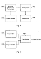
- FIG. 3 is a schematic diagram illustrating a training phase
- Figure 4 is a schematic diagram illustrating a detection phase.
- the present method is based on modelling the face in parts instead of as a whole.
- the parts can either be blocks centred over the assumed positions of the facial features (so-called “selective sampling”) or blocks sampled at regular intervals over the face (so-called “regular sampling”).
- selective sampling blocks centred over the assumed positions of the facial features
- regular sampling blocks sampled at regular intervals over the face
- an analysis process is applied to a set of images known to contain faces, and (optionally) another set of images (“nonface images”) known not to contain faces.
- the analysis process builds a mathematical model of facial and nonfacial features, against which a test image can later be compared (in the detection phase).
- a set of "nonface” images can be used to generate a corresponding set of “nonface” histograms. Then, to achieve detection of a face, the "probability" produced from the nonface histograms may be compared with a separate threshold, so that the probability has to be under the threshold for the test window to contain a face. Alternatively, the ratio of the face probability to the nonface probability could be compared with a threshold.
- Extra training data may be generated by applying "synthetic variations" 330 to the original training set, such as variations in position, orientation, size, aspect ratio, background scenery, lighting intensity and frequency content.
- eigenblocks are core blocks (or eigenvectors) representing different types of block which may be present in the windowed image.
- eigenblocks are core blocks (or eigenvectors) representing different types of block which may be present in the windowed image.
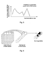
- the generation of eigenblocks will first be described with reference to Figure 6.
- the attributes in the present embodiment are based on so-called eigenblocks.
- the eigenblocks were designed to have good representational ability of the blocks in the training set. Therefore, they were created by performing principal component analysis on a large set of blocks from the training set. This process is shown schematically in Figure 6 and described in more detail in Appendix B.
- a second set of eigenblocks was generated from a much larger set of training blocks. These blocks were taken from 500 face images in the training set. In this case, the 16x 16 blocks were sampled every 8 pixels and so overlapped by 8 pixels. This generated 49 blocks from each 64x64 training image and led to a total of 24,500 training blocks.
- the first 12 eigenblocks generated from these training blocks are shown in Figure 8.
- Empirical results show that eigenblock set II gives slightly better results than set I. This is because it is calculated from a larger set of training blocks taken from face images, and so is perceived to be better at representing the variations in faces. However, the improvement in performance is not large.
- a histogram was built for each sampled block position within the 64x64 face image.
- the number of histograms depends on the block spacing. For example, for block spacing of 16 pixels, there are 16 possible block positions and thus 16 histograms are used.
- the process used to build a histogram representing a single block position is shown in Figure 9.
- the histograms are created using a large training set 400 of M face images. For each face image, the process comprises:
- M is very large, e.g. several thousand. This can more easily be achieved by using a training set made up of a set of original faces and several hundred synthetic variations of each original face.
- a histogram bin number is generated from a given block using the following process, as shown in Figure 10.
- the 16x16 block 440 is extracted from the 64x64 window or face image.
- the block is projected onto the set 450 of A eigenblocks to generate a set of "eigenblock weights".
- These eigenblock weights are the "attributes" used in this implementation. They have a range of-1 to +1. This process is described in more detail in Appendix B .
- the bin “contents”, i.e. the frequency of occurrence of the set of attributes giving rise to that bin number, may be considered to be a probability value if it is divided by the number of training images M. However, because the probabilities are compared with a threshold, there is in fact no need to divide through by M as this value would cancel out in the calculations. So, in the following discussions, the bin “contents” will be referred to as "probability values”, and treated as though they are probability values, even though in a strict sense they are in fact frequencies of occurrence.
- the face detection process involves sampling the test image with a moving 64x64 window and calculating a face probability at each window position.
- the calculation of the face probability is shown in Figure 11.
- the block's bin number 490 is calculated as described in the previous section.
- each bin number is looked up and the probability 510 of that bin number is determined.
- the sum 520 of the logs of these probabilities is then calculated across all the blocks to generate a face probability value, P face (otherwise referred to as a log likelihood value).
- This process generates a probability "map" for the entire test image.
- a probability value is derived in respect of each possible window centre position across the image.
- the combination of all of these probability values into a rectangular (or whatever) shaped array is then considered to be a probability "map" corresponding to that image.
- This map is then inverted, so that the process of finding a face involves finding minima in the inverted map (of course this is equivalent to not inverting the map and finding maxima; either could be done).
- a so-called distance-based technique is used. This technique can be summarised as follows: The map (pixel) position with the smallest value in the inverted probability map is chosen. If this value is larger than a threshold (TD), no more faces are chosen. This is the termination criterion. Otherwise a face-sized block corresponding to the chosen centre pixel position is blanked out (i.e. omitted from the following calculations) and the candidate face position finding procedure is repeated on the rest of the image until the termination criterion is reached.
- TD threshold
- the nonface model comprises an additional set of histograms which represent the probability distribution of attributes in nonface images.
- the histograms are created in exactly the same way as for the face model, except that the training images contain examples of nonfaces instead of faces.
- P combined is then used instead of P face to produce the probability map (before inversion).
- face and non-face histograms may optionally be combined at the end of the training process (prior to face detection) by simply summing log histograms:
- Figures 12a to 12f show some examples of histograms generated by the training process described above.
- Figures 12a, 12b and 12c are derived from a training set of face images
- Figures 12d, 12e and 12f are derived from a training set of nonface images.
- Figure 12b Figure 12e
- a further zoom onto the region about h 1570
- Figure 12c Figure 12f
- the histograms store statistical information about the likelihood of a face at a given scale and location in an image.
- the ordering of the histograms is unexpectedly significant to system performance.
- a simple ordering can result in the access being non-localised (i.e. consecutive accesses are usually far apart in memory). This can give poor cache performance when implemented using microprocessors or bespoke processors.
- the histograms are reordered so that the access to the data are more localised.
- F 38 Frontal face with an eye spacing of 38 pixels that is, a "zoomed in” histogram) L 38 Face facing to the left by 25 degrees, with an eye spacing of 38 pixels R 38 Face facing to the right by 25 degrees, with an eye spacing of 38 pixels
- F 22 Frontal face with an eye spacing of 22 pixels that is, a "full face” histogram) L 22 Face facing to the left by 25 degrees, with an eye spacing of 22 pixels R 22 Face facing to the right by 25 degrees, with an eye spacing of 22 pixels
- F 38 c,x,y is the value of the histogram for a given c,x & y.
- F 38 15,4,5 is the value given by the frontal histogram with the 38 eye spacing at location (4,5) in the face window, for a binmap value of 15.
- a straightforward ordering of the histograms in memory is by c, then x, then y , then pose, and then eye spacing.
- a schematic example of this ordering is shown in Figure 13a.
- An improved ordering system is by pose then x then y then c and then eye spacing.
- a schematic example of this type of ordering is shown in Figure 13b.
- the three different poses are always accessed with the same bin-number and location for each location. i.e. if F 38 329,2,1 is accessed, then L 38 329,2,1 & R 38 329,2,1 are also accessed. These are adjacent in the new method, so excellent cache performance is achieved.
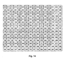
- the new method of organising the histograms also takes advantage of the way that the face window moves during a search for faces in the image. Because of the way that the face window moves the same c value will be looked up in many (x,y) locations.
- Figure 14 shows which values are used from the bin map to look for a face in a certain location.
- F 38 329,2,1 is the value from the frontal histogram for eye spacing 38 for the (2,1) location in the face window.
- the values stored in each histogram bin are quantised to a different number of bits depending on which pose they represent.
- each set of 3 histogram values can be stored in 2 bytes instead of 3.
- the test image is scaled by a range of factors and a distance (i.e. probability) map is produced for each scale.
- a distance map is produced for each scale.
- FIGs 15a to 15c the images and their corresponding distance maps are shown at three different scales.
- the method gives the best response (highest probability, or minimum distance) for the large (central) subject at the smallest scale (Fig 15a) and better responses for the smaller subject (to the left of the main figure) at the larger scales. (A darker colour on the map represents a lower value in the inverted map, or in other words a higher probability of there being a face).
- Candidate face positions are extracted across different scales by first finding the position which gives the best response over all scales.
- the highest probability (lowest distance) is established amongst all of the probability maps at all of the scales.
- This candidate position is the first to be labelled as a face.
- the window centred over that face position is then blanked out from the probability map at each scale.
- the size of the window blanked out is proportional to the scale of the probability map.
- FIGS 15a to 15c Examples of this scaled blanking-out process are shown in Figures 15a to 15c.
- the highest probability across all the maps is found at the left hand side of the largest scale map ( Figure 15c).
- An area 530 corresponding to the presumed size of a face is blanked off in Figure 15c.
- Corresponding, but scaled, areas 532, 534 are blanked off in the smaller maps.
- Areas larger than the test window may be blanked off in the maps, to avoid overlapping detections.
- an area equal to the size of the test window surrounded by a border half as wide/long as the test window is appropriate to avoid such overlapping detections.
- the intervals allowed between the scales processed are influenced by the sensitivity of the method to variations in size. It was found in this preliminary study of scale invariance that the method is not excessively sensitive to variations in size as faces which gave a good response at a certain scale often gave a good response at adjacent scales as well.
- the above description refers to detecting a face even though the size of the face in the image is not known at the start of the detection process.
- Another aspect of multiple scale face detection is the use of two or more parallel detections at different scales to validate the detection process. This can have advantages if, for example, the face to be detected is partially obscured, or the person is wearing a hat etc.
- Figures 15d to 15g schematically illustrate this process.
- the system is trained on windows (divided into respective blocks as described above) which surround the whole of the test face (Figure 15d) to generate "full face” histogram data and also on windows at an expanded scale so that only a central area of the test face is included ( Figure 15e) to generate "zoomed in” histogram data.
- This generates two sets of histogram data. One set relates to the "full face” windows of Figure 15d, and the other relates to the "central face area" windows of Figure 15e.
- the window is applied to two different scalings of the test image so that in one (Figure 15f) the test window surrounds the whole of the expected size of a face, and in the other ( Figure 15g) the test window encompasses the central area of a face at that expected size.
- Figure 15f the test window surrounds the whole of the expected size of a face
- Figure 15g the test window encompasses the central area of a face at that expected size.
- the multiple scales for the arrangements of Figures 15a to 15c are arranged in a geometric sequence.
- each scale in the sequence is a factor of 2 4 different to the adjacent scale in the sequence.
- the larger scale, central area, detection is carried out at a scale 3 steps higher in the sequence, that is, 2 3 ⁇ 4 times larger than the "full face" scale, using attribute data relating to the scale 3 steps higher in the sequence.
- the geometric progression means that the parallel detection of Figures 15d to 15g can always be carried out using attribute data generated in respect of another multiple scale three steps higher in the sequence.
- the two processes can be combined in various ways.
- the multiple scale detection process of Figures 15a to 15c can be applied first, and then the parallel scale detection process of Figures 15d to 15g can be applied at areas (and scales) identified during the multiple scale detection process.
- a convenient and efficient use of the attribute data may be achieved by:
- Further parallel testing can be performed to detect different poses, such as looking straight ahead, looking partly up, down, left, right etc.
- a respective set of histogram data is required and the results are preferably combined using a "max" function, that is, the pose giving the highest probability is carried forward to thresholding, the others being discarded.
- the face detection algorithm provides many probability maps at many scales; the requirement is to find all the places in the image where the probability exceeds a given threshold, whilst ensuring that there are no overlapping faces.
- a disadvantage of the method described above is that it requires the storage of a complete set of probability maps at all scales, which is a large memory requirement.
- the following technique does not require the storage of all of the probability maps simultaneously.
- a temporary list of candidate face locations is maintained. As the probability map for each scale is calculated, the probability maxima are found and compared against the list of candidate face locations to ensure that no overlapping faces exist.
- this method uses a face list to maintain a list of current locations when there might be a face.
- Each face in the face list has a face location and a face size.
- the threshold is the probability threshold above which an object is deemed to be a face.
- the scale factor is the size factor between successive scales (1.189207115 or 2 4 in the present embodiment).
- a 16 x 16 face_size is considered in the example description below.
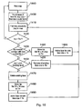
- the process starts at a step 1400 in respect of one of the scales (in the example shown, the smallest scale).
- the face list will be empty, but in general, for all faces in the face list, the face size for each face is modified at the step 1400 by multiplying the respective face size by the scale factor. This makes sure that faces detected in respect of the previous scale are correctly sized for a valid comparison with any maxima in the current scale.
- the maximum probability value, mp is detected in the current map.
- the maximum probability value mp is compared with the threshold. If mp is greater than the threshold then control passes to a step 1430. On the other hand, if mp is not greater than the threshold then processing of the next map (corresponding to the next scale factor to be dealt with) is initiated at a step 1440.
- the value mp is compared with a stored probability value in respect of the existing face. If mp is greater than that probability then the existing face is deleted at a step 1470 and a new entry created in the face list corresponding to the current value and position of mp. In particular, the value mp is stored in respect of the new entry in the face list and a 16x16 pixel area centred on the image position of the current maximum probability is set to the threshold at a step 1480. At a step 1490 the current location of the maximum probability value is added to the face list with a face size of 16. Control then returns to the step 1410.
- step 1460 if the maximum probability location was detected not to overlap with any faces in the face list (at the step 1430) then a new entry is created in the face list.
- the value mp is stored and a 16x16 area surrounding the current maximum value is set to the threshold.
- the current maximum position is added to the face list with a face size of 16 and control returns to the step 1410.
- a maximum probability value mp is again detected, but this will be in the light of modifications to the probability values surrounding detected faces in the steps 1460, 1455 and 1480. So, the modified values created at those steps will not in fact pass the test of the step 1420, in that a value set to equal the threshold value will be found not to exceed it. Accordingly, the step 1420 will establish whether another position exists in the correct map where the threshold value is exceeded.
- An advantage of this method is that it allows each scale of probability map to be considered separately. Only the face list needs to be stored in between processing each scale. This has the following advantages:
- a change detection process is used to detect which areas of the image have changed since the previous frame, or at least to remove from the face detection process certain areas detected not to have changed since the previous frame.
- Areas of the image that have not changed since the previous frame do not need to have face detection performed on them again, as the result is likely to be the same as the previous frame. However, areas of the images that have changed need to have face detection performed on them afresh. These areas of the image are labelled as "areas of interest" during change detection.
- change detection is performed only at a single fixed scale, e.g. the original image scale or the largest scale that is used in face detection.
- a single fixed scale e.g. the original image scale or the largest scale that is used in face detection.
- Figure 17 which schematically illustrates a motion detector.
- the current and previous frames are first processed by low pass filters 1100, 1110.
- the two frames are then supplied to a differencer 1120 to produce a frame difference image, for example a representation of the absolute pixel (or block) differences between frames with one difference value per pixel (or block) position.
- the absolute values of the difference image are then thresholded 1130 by comparison with a threshold value Thr diff to create a binary difference image, i.e. an array of one-bit values with one value per pixel (or block) position: very small differences are set to zero (no change) and larger differences are set to one (change detected).
- a morphological opening operation is performed 1140 on the binary difference image to create more contiguous areas of detected change/motion.
- the low-pass filtering operation may be omitted.
- Morphological opening is a known image processing technique and in this example is performed on a 3x3 area (i.e. a 3x3 block is used as the morphological structuring element) and comprises a morphological erosion operation followed by a morphological dilation operation.
- the morphological processing is carried out after processing every third line.
- Change detection can be applied to the whole image, as described above, to create a map of areas of the image where changes have been detected. Face detection is applied to those areas.
- change detection can be used to eliminate certain areas of the image from face detection, though without necessarily detecting all areas of motion or "no motion". This technique has the advantage of reducing the processing requirements of the change detection process while still potentially providing a useful saving in processing for the face detection itself.
- a schematic example of this process is illustrated in Figures 18a to 18e.
- the scan 1150 progresses until the detected absolute difference in respect of one scan position 1160 exceeds the threshold Thr diff . At this point the scan 1150 terminates.
- the scan 1170 is a horizontal scan starting at the bottom of the image and terminates when a scan position 1200 gives rise to an absolute difference value exceeding the threshold Thr diff .
- the scan 1180 is a downwards vertical scan starting at the left hand side of the image and terminates when a scan position 1210 gives rise to an absolute difference value exceeding the threshold Thr diff .
- the scan 1190 is a downwards vertical scan starting at the right hand side of the image and terminates when a scan position 1220 gives rise to an absolute difference value exceeding the threshold Thr diff .
- the four points 1160, 1200, 1210, 1220 define a bounding box 1230 in Figure 18e.
- the four vertices of the bounding box 1230 are given by: top left (x 1210 , y 1160 ) top right (x 1220 , y 1160 ) bottom left (x 1210 , y 1200 ) bottom right (x 1220 , y 1200 )
- the bounding box therefore does not define all areas of the image in which changes have been detected, but instead it defines an area (outside the bounding box) which can be excluded from face processing because change has not been detected there.
- an area outside the bounding box
- the area inside the bounding box potentially all of the area may have changed, but a more usual situation would be that some parts of that area may have changed and some not.
- the two vertical scans 1180', 1190' are carried out only in respect of those rows 1240 which have not already been eliminated by the two horizontal scans 1150, 1170. This variation can reduce the processing requirements.
- change detection is carried out, starting from four extremes (edges) of the image, and stops in each case when a change is detected. So, apart from potentially the final pixel (or block) or part row/column of each of the change detection processes, change detection is carried out only in respect of those image areas which are not going to be subject to face detection. Similarly, apart from that final pixel, block or part row/column, face detection is carried out only in respect of areas which have not been subject to the change detection process. Bearing in mind that change detection is less processor-intensive than face detection, this relatively tiny overlap between the two processes means that in almost all situations the use of change detection will reduce the overall processing requirements of an image.
- a different method of change detection applies to motion-encoded signals such as MPEG-encoded signals, or those which have been previously encoded in this form and decoded for face detection.
- Motion vectors or the like associated with the signals can indicate where an inter-image change has taken place.
- a block (e.g. an MPEG macroblock) at the destination (in a current image) of each motion vector can be flagged as an area of change. This can be done instead of or in addition to the change detection techniques described above.
- Another method of reducing the processing requirements is as follows.
- the face detection algorithm is divided into a number of stages that are repeated over many scales.
- the algorithm is only completed after n calls.
- the algorithm is automatically partitioned so that each call takes approximately an equal amount of time.
- the key features of this method are:
- Process Scale Description Motion 1 Motion is used to reduce search area Variance 1 Image variance is used to reduce search area Decimate 1 ⁇ 2 Image is reduced in size to next scale Convolve 2 Image is convolved to produce bin-map Decimate 2 ⁇ 3 Convolve 3 Decimate 3 ⁇ 4 Convolve 4 Lookup 4 Bin-maps are used to lookup face probabilities Max-Search 4 Maximum probabilities are found and thresholded Decimate 4 ⁇ 5 Convolve 5 Lookup 5 Max-Search 5 Decimate 5 ⁇ 6 Convolve 6 Lookup 6 Max-Search 6 Tracking -
- the following table shows what might happen if a temporal decimation of 4 is used.
- the algorithm automatically divides up the processing into 'chunks' of equal time - this is complicated by the fact that the processing for the earlier scales requires more time than the processing for later scales (the images being larger for the earlier scales).
- the algorithm estimates the amount of time that each stage will require before carrying it out. This estimate is given by the particular process and the number of pixels to be processed for a given scale.
- the system calculates whether the number of cumulated processing units required will take it over some prearranged level (5300 for example). If it does, then a return is carried out without executing this stage. This has the advantage over timing that it is known in advance of doing something whether it will exceed the allotted time.
- Horizontal striping was chosen because it is considered more efficient to process horizontal stripes, although any sort of division could be used (squares, vertical stripes etc.)
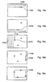
- Figures 20a to 20c schematically illustrate a striping technique.
- no spatial decimation is used and the entire image 1300 is subjected to face detection.
- the image is split into two portions 1310, 1320. These are each subjected to face detection in alternate images.
- the image is split into three portions 1330, 1340, 1350 so that each portion is subjected to face detection for one in every three images. The portions may be distinct or may overlap slightly.
- FIGS. 21 a to 12d schematically illustrate so-called sparse spatial decimation. Three variables are defined:
- Figures 21 a to 21 d are as follows: Figure 21a Figure 21b Figure 21c Figure 21d SparseX 2 2 2 2 SparseY 1 1 2 2 UseChequerBoard 0 1 0 1
- a combination of spatial and temporal decimation can be used. For example, discrete spatial portions of an image (e.g. a third of an image) could be processed over a number of frames. The portions (e.g. the three thirds) processed in this way could come from the same image or from different respective images.
- the tracking algorithm aims to improve face detection performance in image sequences.
- the initial aim of the tracking algorithm is to detect every face in every frame of an image sequence. However, it is recognised that sometimes a face in the sequence may not be detected. In these circumstances, the tracking algorithm may assist in interpolating across the missing face detections.
- the goal of face tracking is to be able to output some useful metadata from each set of frames belonging to the same scene in an image sequence. This might include:
- input video data 545 (representing the image sequence) is supplied to a face detector of the type described in this application, and a skin colour matching detector 550.
- the face detector attempts to detect one or more faces in each image.
- a Kalman filter 560 is established to track the position of that face.
- the Kalman filter generates a predicted position for the same face in the next image in the sequence.
- An eye position comparator 570, 580 detects whether the face detector 540 detects a face at that position (or within a certain threshold distance of that position) in the next image. If this is found to be the case, then that detected face position is used to update the Kalman filter and the process continues.
- a skin colour matching method 550 is used. This is a less precise face detection technique which is set up to have a lower threshold of acceptance than the face detector 540, so that it is possible for the skin colour matching technique to detect (what it considers to be) a face even when the face detector cannot make a positive detection at that position. If a "face" is detected by skin colour matching, its position is passed to the Kalman filter as an updated position and the process continues.
- the predicted position is used to update the Kalman filter.
- a separate Kalman filter is used to track each face in the tracking algorithm.
- a state model representing the face In order to use a Kalman filter to track a face, a state model representing the face must be created.
- the position of each face is represented by a 4-dimensional vector containing the co-ordinates of the left and right eyes, which in turn are derived by a predetermined relationship to the centre position of the window and the scale being used:
- p ( k ) [ FirstEye X FirstEye Y SecondEye X SecondEye Y ] where k is the frame number.
- the tracking algorithm does nothing until it receives a frame with a face detection result indicating that there is a face present.
- the state model error covariance, Q and the observation error covariance, R are also assigned some other attributes: the state model error covariance, Q and the observation error covariance, R.
- the error covariance of the Kalman filter, P is also initialised. These parameters are described in more detail below. At the beginning of the following frame, and every subsequent frame, a Kalman filter prediction process is carried out.
- the filter uses the previous state (at frame k-1) and some other internal and external variables to estimate the current state of the filter (at frame k).
- State prediction equation: z ⁇ b ( k ) ⁇ ( k , k ⁇ 1 ) z ⁇ a ( k ⁇ 1 )
- Covariance prediction equation: P b ( k ) ⁇ ( k , k ⁇ 1 ) P a ( k ⁇ 1 ) ⁇ ( k , k ⁇ 1 ) T + Q ( k )
- ⁇ b (k) denotes the state before updating the filter for frame k
- ⁇ a ( k-1 ) denotes the state after updating the filter for frame k -1 (or the initialised state if it is a new filter)
- ⁇ ( k,k- 1) is the state transition matrix.
- P b ( k ) denotes the filter's error covariance before updating the filter for frame k
- P a ( k -1) denotes the filter's error covariance after updating the filter for the previous frame (or the initialised value if it is a new filter).
- P b ( k ) can be thought of as an internal variable in the filter that models its accuracy.
- Q(k) is the error covariance of the state model.
- a high value of Q(k) means that the predicted values of the filter's state (i.e. the face's position) will be assumed to have a high level of error.
- the state transition matrix, ⁇ (k, k -1), determines how the prediction of the next state is made.
- ⁇ t can simply be set to 1 (i.e. units of t are frame periods).
- the predicted eye positions of each Kalman filter, ⁇ b ( k ), are compared to all face detection results in the current frame (if there are any). If the distance between the eye positions is below a given threshold, then the face detection can be assumed to belong to the same face as that being modelled by the Kalman filter.
- Skin colour matching is not used for faces that successfully match face detection results. Skin colour matching is only performed for faces whose position has been predicted by the Kalman filter but have no matching face detection result in the current frame, and therefore no observation data to help update the Kalman filter.
- an elliptical area centred on the face's previous position is extracted from the previous frame.
- An example of such an area 600 within the face window 610 is shown schematically in Figure 24.
- a colour model is seeded using the chrominance data from this area to produce an estimate of the mean and covariance of the Cr and Cb values, based on a Gaussian model.
- Figures 23a and 23b schematically illustrate the generation of the search area.
- Figure 23a schematically illustrates the predicted position 620 of a face within the next image 630.
- a search area 640 surrounding the predicted position 620 in the next image is searched for the face.
- the skin colour matching methods described above use a simple Gaussian skin colour model.
- the model is seeded on an elliptical area centred on the face in the previous frame, and used to find the best matching elliptical area in the current frame.
- two further methods were developed: a colour histogram method and a colour mask method. These will now be described.
- a histogram of Cr and Cb values within a square window around the face is computed. To do this, for each pixel the Cr and Cb values are first combined into a single value. A histogram is then computed that measures the frequency of occurrence of these values in the whole window. Because the number of combined Cr and Cb values is large (256x256 possible combinations), the values are quantised before the histogram is calculated.
- the histogram is used in the current frame to try to estimate the most likely new position of the face by finding the area of the image with the most similar colour distribution. As shown schematically in Figures 23a and 23b, this is done by calculating a histogram in exactly the same way for a range of window positions within a search area of the current frame. This search area covers a given area around the predicted face position. The histograms are then compared by calculating the mean squared error (MSE) between the original histogram for the tracked face in the previous frame and each histogram in the current frame. The estimated position of the face in the current frame is given by the position of the minimum MSE.
- MSE mean squared error
- This method is based on the method first described above. It uses a Gaussian skin colour model to describe the distribution of pixels in the face.
- an elliptical area centred on the face is used to colour match faces, as this may be perceived to reduce or minimise the quantity of background pixels which might degrade the model.
- a similar elliptical area is still used to seed a colour model on the original tracked face in the previous frame, for example by applying the mean and covariance of RGB or YCrCb to set parameters of a Gaussian model (or alternatively, a default colour model such as a Gaussian model can be used, see below).
- a mask area is calculated based on the distribution of pixels in the original face window from the previous frame. The mask is calculated by finding the 50% of pixels in the window which best match the colour model.
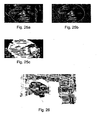
- Figures 25a to 25c An example is shown in Figures 25a to 25c.
- Figure 25a schematically illustrates the initial window under test
- Figure 25b schematically illustrates the elliptical window used to seed the colour model
- Figure 25c schematically illustrates the mask defined by the 50% of pixels which most closely match the colour model.
- a search area around the predicted face position is searched (as before) and the "distance" from the colour model is calculated for each pixel.
- the "distance” refers to a difference from the mean, normalised in each dimension by the variance in that dimension.
- An example of the resultant distance image is shown in Figure 26.
- the pixels of the distance image are averaged over a mask-shaped area. The position with the lowest averaged distance is then selected as the best estimate for the position of the face in this frame.
- This method thus differs from the original method in that a mask-shaped area is used in the distance image, instead of an elliptical area. This allows the colour match method to use both colour and shape information.
- Gaussian skin colour models will now be described further.
- a Gaussian model for the skin colour class is built using the chrominance components of the YCbCr colour space.
- the similarity of test pixels to the skin colour class can then be measured.
- This method thus provides a skin colour likelihood estimate for each pixel, independently of the eigenface-based approaches.
- w be the vector of the CbCr values of a test pixel.
- the probability of w belonging to the skin colour class S is modelled by a two-dimensional Gaussian: p ( w
- S ) exp [ ⁇ 1 2 ( w ⁇ ⁇ s ) ⁇ s ⁇ 1 ( w ⁇ ⁇ s ) ] 2 ⁇
- Skin colour detection is not considered to be an effective face detector when used on its own. This is because there can be many areas of an image that are similar to skin colour but are not necessarily faces, for example other parts of the body. However, it can be used to improve the performance of the eigenblock-based approaches by using a combined approach as described in respect of the present face tracking system.
- the decisions made on whether to accept the face detected eye positions or the colour matched eye positions as the observation for the Kalman filter, or whether no observation was accepted, are stored. These are used later to assess the ongoing validity of the faces modelled by each Kalman filter.
- the update step is used to determine an appropriate output of the filter for the current frame, based on the state prediction and the observation data. It also updates the internal variables of the filter based on the error between the predicted state and the observed state.
- Kalman gain equation K ( k ) P b ( k ) H T ( k ) ( H ( k ) P b ( k ) H T ( k ) + R ( k ) ) ⁇ 1
- State update equation z ⁇ a ( k ) z ⁇ b ( k ) + K ( k ) [ y ( k ) ⁇ H ( k ) z ⁇ b ( k ) ]
- Covariance update equation P a ( k ) P b ( k ) ⁇ K ( k ) H ( k ) P b ( k )
- K(k) denotes the Kalman gain, another variable internal to the Kalman filter. It is used to determine how much the predicted state should be adjusted based on the observed state, y(k).
- R(k) is the error covariance of the observation data.
- a high value of R(k) means that the observed values of the filter's state (i.e. the face detection results or colour matches) will be assumed to have a high level of error.
- the behaviour of the filter can be changed and potentially improved for face detection.
- a large value of R(k) relative to Q(k) was found to be suitable (this means that the predicted face positions are treated as more reliable than the observations). Note that it is permissible to vary these parameters from frame to frame. Therefore, an interesting future area of investigation may be to adjust the relative values of R(k) and Q(k) depending on whether the observation is based on a face detection result (reliable) or a colour match (less reliable).
- the updated state, ⁇ o ( k ) is used as the final decision on the position of the face. This data is output to file and stored.
- the associated Kalman filter is removed and no data is output to file.
- the tracking results up to the frame before it leaves the picture may be stored and treated as valid face tracking results (providing that the results meet any other criteria applied to validate tracking results).
- the tracking process is not limited to tracking through a video sequence in a forward temporal direction. Assuming that the image data remain accessible (i.e. the process is not real-time, or the image data are buffered for temporary continued use), the entire tracking process could be carried out in a reverse temporal direction. Or, when a first face detection is made (often part-way through a video sequence) the tracking process could be initiated in both temporal directions. As a further option, the tracking process could be run in both temporal directions through a video sequence, with the results being combined so that (for example) a tracked face meeting the acceptance criteria is included as a valid result whichever direction the tracking took place.
- a face track is started for every face detection that cannot be matched up with an existing track. This could lead to many false detections being erroneously tracked and persisting for several frames before finally being rejected by one of the existing rules (e.g. prediction_acceptance_ratio_threshold)
- the rules for rejecting a track e.g. prediction_acceptance_ratio threshold, detection_acceptance_ratio_threshold
- prediction_acceptance_ratio threshold e.g. prediction_acceptance_ratio threshold, detection_acceptance_ratio_threshold
- the first part of the solution helps to prevent false detections from setting off erroneous tracks.
- a face track is still started internally for every face detection that does not match an existing track. However, it is not output from the algorithm.
- the first f frames in the track must be face detections (i.e. of type D ). If all of the first f frames are of type D then the track is maintained and face locations are output from the algorithm from frame f onwards. If all of the first n frames are not of type D, then the face track is terminated and no face locations are output for this track.
- f is typically set to 2, 3 or 5.
- the second part of the solution allows faces in profile to be tracked for a long period, rather than having their tracks terminated due to a low detection_acceptance_ratio.
- prediction_acceptance_ratio_threshold and detection_acceptance _ratio _threshold are not turned on in this case.
- prediction_acceptance_ratio_threshold and detection_acceptance_ratio_threshold rules may also be combined with the prediction_acceptance_ratio_threshold and detection_acceptance_ratio_threshold rules.
- the prediction_acceptance_ratio_threshold and detection_acceptance_ratio_threshold may be applied on a rolling basis e.g. over only the last 30 frames, rather than since the beginning of the track.
- the skin colour of the face is only checked during skin colour tracking. This means that non-skin-coloured false detections may be tracked, or the face track may wander off into non-skin-coloured locations by using the predicted face position.
- An efficient way to implement this is to use the distance from skin colour of each pixel calculated during skin colour tracking. If, this measure averaged over the face area (either over a mask shaped area, over an elliptical area or over the whole face window depending on which skin colour tracking method is being used), exceeds a fixed threshold, then the face track is terminated.
- an area of interest pre-processor is used to ascertain which areas of the image have non-face-like variance. This is repeated at every scale, and these areas are then omitted from face detection processing. However, it is still possible for a skin colour tracked or Kalman predicted face to move into a (non-face-like) low or high variance area of the image.
- the variance values (or gradient values) for the areas around existing face tracks are stored.
- the position is validated against the stored variance (or gradient) values in the area of interest map. If the position is found to have very high or very low variance (or gradient), it is considered to be non-face-like and the face track is terminated. This avoids face tracks wandering onto low (or high) variance background areas of the image. Alternatively, the variance of the new face position is calculated afresh (useful if variance-pre-processing is not used).
- variance measure used can either be traditional variance or the sum of differences of neighbouring pixels (gradient) or any other variance-type measure.
- Shot boundary data 560 (from metadata associated with the image sequence under test; or metadata generated within the camera of Figure 2) defines the limits of each contiguous "shot” within the image sequence.
- the Kalman filter is reset at shot boundaries, and is not allowed to carry a prediction over to a subsequent shot, as the prediction would be meaningless.
- User metadata 542 and camera setting metadata 544 are supplied as inputs to the face detector 540. These may also be used in a non-tracking system. Examples of the camera setting metadata were described above.
- User metadata may include information such as:
- the type of programme is relevant to the type of face which may be expected in the images or image sequence. For example, in a news programme, one would expect to see a single face for much of the image sequence, occupying an area of (say) 10% of the screen.
- the detection of faces at different scales can be weighted in response to this data, so that faces of about this size are given an enhanced probability.
- Another alternative or additional approach is that the search range is reduced, so that instead of searching for faces at all possible scales, only a subset of scales is searched. This can reduce the processing requirements of the face detection process.
- the software can run more quickly and/or on a less powerful processor.
- a hardware-based system including for example an application-specific integrated circuit (ASIC) or field programmable gate array (FPGA) system
- the hardware needs may be reduced.
- the other types of user metadata mentioned above may also be applied in this way.
- the "expected face size" sub-ranges may be stored in a look-up table held in the memory 30, for example.
- camera metadata for example the current focus and zoom settings of the lens 110
- these can also assist the face detector by giving an initial indication of the expected image size of any faces that may be present in the foreground of the image.
- the focus and zoom settings between them define the expected separation between the camcorder 100 and a person being filmed, and also the magnification of the lens 110. From these two attributes, based upon an average face size, it is possible to calculate the expected size (in pixels) of a face in the resulting image data, leading again to a subrange of sizes for search or a weighting of the expected face sizes.
- the face tracking technique has three main benefits:
- Variation 1 a default Gaussian skin colour model is used to calculate the colour distance value for every pixel in the image (to give a colour distance map).
- a face When a face is detected, its average distance from the default is calculated over a mask shaped area.
- the face track is terminated if the distance from the default colour model varies outside a given tolerance. This means (a) the same colour distance values can be used for all face tracks (there is no need for a different model for each face, since we use default colour model rather than seeding on face colour) and (b) if track wanders off face onto a different coloured background it is terminated, rather than persisting.
- Variation 2 instead of a default colour model, a different colour model is used for each face, seeded on that face's colour when it is first detected. Then, when the colour distance map is calculated, different colour model parameters are used in different areas of the image, dependent on the position of each face in the previous frame. The colour distance values may be blended together as a weighted sum on areas in between two faces. This allows the colour tracking to be modelled more accurately on each face's actual colour without needing to calculate more than one colour distance value for each pixel position in the image.
- Variation 3 instead of a default colour model, or different colour models for each face, a general colour model is seeded on the average colour of all detected faces from the previous frame.
- Variation 4 when searching the colour distance map with a square head-sized window to find the minimum averaged distance from skin colour, areas inside the mask give a positive contribution and areas outside the mask give a negative contribution. This means that plain, skin coloured areas should have a net distance from skin colour of zero. It also means that the shape-matching property of the mask method is reinforced. In the method described above, only areas inside the face mask were used.
- Variation 5 the colour distance map is first quantised to two levels so that each pixel is either skin colour (1) or non-skin colour (-1). This prevents the magnitude of the colour distance values from having an undue effect on the distance from skin colour calculation, i.e. when combined with variation 4 above, very non-skin coloured pixels outside the mask do not have an undue influence.
- Variation 6 the skin colour mask is updated more gradually.
- a new mask is calculated as 90% of the previous frame's mask with only a 10% weighting of the current frame's mask. This helps to avoid the problems caused by temporary partial occlusions, e.g. hands passing briefly in front of the face. Also helps to avoid problem of people moving very slowly.
- the skin colour tracking technique described earlier worked by matching the colour distance mask of the face in the previous frame to the colour distance map of the current frame.
- This method which at least some of the variations aim to improve:
- Variation 6 in which the colour distance mask for the face is only slowly updated, addresses aspects (i) and (ii). As well as getting a good match for skin colour areas within the facemask, non face coloured areas are also considered in Variation 5, which addresses (iii).
- a binary mask is calculated from the previous frame's colour distance map at the location of the face within this frame.
- Each element of the mask is either '1' if it is less than the average colour distance value for the entire mask (i.e. it is skin coloured), or else '0' (non-skin-coloured).
- a search is conducted over the search window using the binary mask. At each point within the search window, a value is calculated by summing all the colour distance values where the mask is '1' and subtracting all the colour distance values where the mask is '0'. The best match is taken to be the position at which the mask gives the minimum summed colour distance value.
- the current colour distance map (for frame n) is updated by summing 90% of the old colour distance map at the old face location 1500 with 10% of the new colour distance map at the new face location 1510.
- searching takes place over a 4x4 grid (i.e. the searching cannot be more accurate than 4 pixels), using the earlier method. If the face moves 1 pixel the searching algorithm will find the face in the same (previous) location. Since the colour distance map was completely replaced with the new one, if the face continues to move at 1 pixel a frame, after 4 frames the face will still be found in the original location, even though it should have now moved 4 pixels - in other words, the mask has 'slipped' from the face.
- each pixel in the map is set to -1 if it is below the average colour distance value of the mask and to +1 if it is above the average colour distance value of the mask (the "average colour distance of the mask” refers to the average colour distance of the face window before it was quantised to 1's and '0's to form the mask).
- a value is calculated at each point within the search window by summing all the colour distance values where the mask is '1' and subtracting all the colour distance values where the mask is '0'.
- these values are calculated and summed for a face-sized window.
- the best match is taken as the pixel location where the minimum value is obtained, i.e. where the mask best matches the image.
- This method prevents the magnitude of the colour distance values from having an undue effect on the distance from skin colour calculation so that very non-skin coloured pixels outside the mask do not have undue influence.
- Figures 29a to 29c schematically illustrate a gradient pre-processing technique.
- a pre-processing step is proposed to remove areas of little pixel variation from the face detection process.
- the pre-processing step can be carried out at each scale.
- the basic process is that a "gradient test" is applied to each possible window position across the whole image.
- a predetermined pixel position for each window position such as the pixel at or nearest the centre of that window position, is flagged or labelled in dependence on the results of the test applied to that window. If the test shows that a window has little pixel variation, that window position is not used in the face detection process.
- FIG 29a A first step is illustrated in Figure 29a. This shows a window at an arbitrary window position in the image. As mentioned above, the pre-processing is repeated at each possible window position. Referring to Figure 29a, although the gradient pre-processing could be applied to the whole window, it has been found that better results are obtained if the pre-processing is applied to a central area 1000 of the test window 1010.
- a gradient-based measure is derived from the window (or from the central area of the window as shown in Figure 29a), which is the average of the absolute differences between all adjacent pixels 1011 in both the horizontal and vertical directions, taken over the window.
- Each window centre position is labelled with this gradient-based measure to produce a gradient "map" of the image.
- the resulting gradient map is then compared with a threshold gradient value. Any window positions for which the gradient-based measure lies below the threshold gradient value are excluded from the face detection process in respect of that image.
- the gradient-based measure is preferably carried out in respect of pixel luminance values, but could of course be applied to other image components of a colour image.
- Figure 29c schematically illustrates a gradient map derived from an example image.
- a lower gradient area 1070 (shown shaded) is excluded from face detection, and only a higher gradient area 1080 is used.
- the embodiments described above have related to a face detection system (involving training and detection phases) and possible uses for it in a camera-recorder and an editing system. It will be appreciated that there are many other possible uses of such techniques, for example (and not limited to) security surveillance systems, media handling in general (such as video tape recorder controllers), video conferencing systems, IP cameras, digital stills cameras and the like.
- window positions having high pixel differences can also be flagged or labelled, and are also excluded from the face detection process.
- a "high" pixel difference means that the measure described above with respect to Figure 29b exceeds an upper threshold value.
- a gradient map is produced as described above. Any positions for which the gradient measure is lower than the (first) threshold gradient value mentioned earlier are excluded from face detection processing, as are any positions for which the gradient measure is higher than the upper threshold value.
- the "lower threshold” processing is preferably applied to a central part 1000 of the test window 1010.
- the same can apply to the "upper threshold” processing. This would mean that only a single gradient measure needs to be derived in respect of each window position.
- the whole window is used in respect of the lower threshold test, the whole window can similarly be used in respect of the upper threshold test. Again, only a single gradient measure needs to be derived for each window position.
- a further criterion for rejecting a face track is that its variance or gradient measure is very low or very high.
- the position is validated against the stored variance (or gradient) values in the area of interest map. If the position is found to have very high or very low variance (or gradient), it is considered to be non-face-like and the face track is terminated. This prevents face tracks from wandering onto low (or high) variance background areas of the image.
- the variance of the new face position can be calculated afresh.
- the variance measure used can either be traditional variance or the sum of differences of neighbouring pixels (gradient) or any other variance-type measure.
- one or more rectangular bounding boxes are placed around the areas of detected motion (or at least, so as to exclude areas which have no detected motion). These boxes are then rescaled to all the scales at which face detection is to be carried out.
- the area of interest decision which is to say a decision as to which areas are to be subjected to face detection, is based on the outputs from the variance pre-processing and change detection processes.
- the area of interest decision logic combines the areas of interest from the variance pre-processing and change detection modules to produce a final area of interest. These are constrained by one or more rectangular bounding boxes at each scale or (without limitation to bounding boxes) a multi-scale "area of interest" map, with each pixel position being labelled as an area of interest or not.
- One database consists of many thousand images of subjects standing in front of an indoor background.
- Another training database used in experimental implementations of the above techniques consists of more than ten thousand eight-bit greyscale images of human heads with views ranging from frontal to left and right profiles.
- the skilled man will of course understand that various different training sets could be used, optionally being profiled to reflect facial characteristics of a local population.
- each m-by-n face image is reordered so that it is represented by a vector of length mn.
- Each image can then be thought of as a point in mn-dimensional space.
- a set of images maps to a collection of points in this large space.
- PCA principal component analysis
- eigenblocks or eigenvectors relating to blocks of the face image.
- a grid of blocks is applied to the face image (in the training set) or the test window (during the detection phase) and an eigenvector-based process, very similar to the eigenface process, is applied at each block position. (Or in an alternative embodiment to save on data processing, the process is applied once to the group of block positions, producing one set of eigenblocks for use at any block position).
- some blocks such as a central block often representing a nose feature of the image, may be more significant in deciding whether a face is present.
- A is an N x N diagonal matrix with the eigenvalues, ⁇ i , along its diagonal (in order of magnitude) and P is an N x N matrix containing the set of N eigenvectors, each of length N .
- This decomposition is also known as a Karhunen-Loeve Transform (KLT).
- the eigenvectors can be thought of as a set of features that together characterise the variation between the blocks of the face images. They form an orthogonal basis by which any image block can be represented, i.e. in principle any image can be represented without error by a weighted sum of the eigenvectors.
- N T ⁇ N the dimension of the space
- the image blocks in the training set are similar in overall configuration (they are all derived from faces), only some of the remaining eigenvectors will characterise very strong differences between the image blocks. These are the eigenvectors with the largest associated eigenvalues. The other remaining eigenvectors with smaller associated eigenvalues do not characterise such large differences and therefore they are not as useful for detecting or distinguishing between faces.
- PCA only the M principal eigenvectors with the largest magnitude eigenvalues are considered, where M ⁇ N T i.e. a partial KLT is performed.
- PCA extracts a lower-dimensional subspace of the KLT basis corresponding to the largest magnitude eigenvalues.
- eigenblocks Because the principal components describe the strongest variations between the face images, in appearance they may resemble parts of face blocks and are referred to here as eigenblocks. However, the term eigenvectors could equally be used.
- the similarity of an unknown image to a face, or its faceness, can be measured by determining how well the image is represented by the face space. This process is carried out on a block-by-block basis, using the same grid of blocks as that used in the training process.
- the first stage of this process involves projecting the image into the face space.
- Blocks of similar appearance will have similar sets of weights while blocks of different appearance will have different sets of weights. Therefore, the weights are used here as feature vectors for classifying face blocks during face detection.
Landscapes
- Engineering & Computer Science (AREA)
- Theoretical Computer Science (AREA)
- Physics & Mathematics (AREA)
- Health & Medical Sciences (AREA)
- General Physics & Mathematics (AREA)
- Oral & Maxillofacial Surgery (AREA)
- Multimedia (AREA)
- General Health & Medical Sciences (AREA)
- Human Computer Interaction (AREA)
- Evolutionary Computation (AREA)
- Artificial Intelligence (AREA)
- Computer Vision & Pattern Recognition (AREA)
- Geometry (AREA)
- Medical Informatics (AREA)
- Databases & Information Systems (AREA)
- Computing Systems (AREA)
- Data Mining & Analysis (AREA)
- Software Systems (AREA)
- Bioinformatics & Cheminformatics (AREA)
- General Engineering & Computer Science (AREA)
- Evolutionary Biology (AREA)
- Bioinformatics & Computational Biology (AREA)
- Life Sciences & Earth Sciences (AREA)
- Image Analysis (AREA)
- Image Processing (AREA)
Claims (19)
- Objekterkennungsvorrichtung (10, 100) zum Erkennen von Objekten in einem Prüfbild, wobei die Vorrichtung aufweist:eine Einrichtung (230) zum Vergleichen von Blöcken eines Prüffensters des Bildes mit Referenzdaten, die die Anwesenheit eines Objekts anzeigen, um Indexpunktzahlen zu erzeugen, die einen Ähnlichkeitsgrad zwischen einem Bereich und den Referenzdaten angeben;eine Einrichtung zum Speichern von Wahrscheinlichkeitsdaten entsprechend möglichen Werten der Indexpunktzahl und der Blockposition;eine Einrichtung, die bezüglich eines aktuellen Blocks zum Zugreifen auf einen Wahrscheinlichkeitswert aus der Speichereinrichtung in Abhängigkeit von dieser Blockposition im Prüffenster und der bezüglich dieses Blocks erzeugten Indexpunktzahl ausgebildet ist; undeine Einrichtung zum Kombinieren der Wahrscheinlichkeitswerte entsprechend den Blöcken in einem Prüffenster, um ein Ergebnis zu erzeugen, das die Wahrscheinlichkeit angibt, dass das Prüffenster ein Objekt enthält,und gekennzeichnet durch
eine Zugriffseinrichtung, die ausgebildet ist, um auf zwei oder mehr Wahrscheinlichkeitswerte bezüglich einer aktuellen Blockposition und Indexpunktzahl zuzugreifen, wobei die zwei oder mehr Wahrscheinlichkeitswerte sich auf verschiedene Objektorientierungen beziehen. - Vorrichtung nach Anspruch 1, bei welcher die Wahrscheinlichkeitswerte in der Speichereinrichtung nach Objektorientierung, Blockposition und dann nach Indexpunktzahl geordnet sind.
- Vorrichtung nach Anspruch 1 oder 2, bei welcher die Kombinationseinrichtung ausgebildet ist, um die Wahrscheinlichkeitswerte betreffend einzelne Objektorientierungen zu kombinieren, um ein jeweiliges Ergebnis für jede Objektorientierung zu erzeugen.
- Vorrichtung nach einem der vorherigen Ansprüche, bei welcher die Wahrscheinlichkeitswerte in der Speichereinrichtung nach Objektorientierung, dann nach Blockposition, dann nach Indexpunktzahl geordnet sind.
- Vorrichtung nach einem der vorherigen Ansprüche, bei welcher die Objektorientierungen wenigstens eine Frontalorientierung und ein zu einer Seite gedrehtes Objekt aufweisen.
- Vorrichtung nach Anspruch 5, bei welcher die Objektorientierungen wenigstens eine Frontalorientierung, ein zu einer Seite gedrehtes Objekt und ein zur anderen Seite gedrehtes Objekt aufweisen.
- Vorrichtung nach Anspruch 5 oder Anspruch 6, bei welcher die Wahrscheinlichkeitswerte betreffend die Frontalorientierung in der Speichereinrichtung mit einer höheren Auflösung als die Wahrscheinlichkeitswerte betreffend die anderen Objektorientierungen gespeichert sind.
- Vorrichtung nach Anspruch 7, bei welcher die Wahrscheinlichkeitswerte betreffend die Frontalorientierung in der Speichereinrichtung mit der doppelten Auflösung der Wahrscheinlichkeitswerte betreffend die anderen Objektorientierungen gespeichert sind.
- Vorrichtung nach einem der vorherigen Ansprüche, bei welcher die Vergleichseinrichtung ausgebildet ist, um die Blöcke auf einen oder mehrere Bildeigenvektoren zu projizieren.
- Vorrichtung nach einem der vorherigen Ansprüche, bei welcher die Zugriffseinrichtung einen Cache-Speicher zum Speichern von kürzlich zugegriffenen Wahrscheinlichkeitswerten und Wahrscheinlichkeitswerten, die in der Speicherreihenfolge nahe den kürzlich zugegriffenen Wahrscheinlichkeitswerten liegen, aufweist.
- Vorrichtung nach einem der vorherigen Ansprüche, bei welcher die Objekte Gesichter sind.
- Videokonferenzvorrichtung mit einer Vorrichtung nach einem der vorherigen Ansprüche.
- Überwachungsvorrichtung mit einer Vorrichtung nach einem der Ansprüche 1 bis 11.
- Kameraanordnung mit einer Vorrichtung nach einem der Ansprüche 1 bis 11.
- Verfahren zum Erkennen von Objekten in einem Prüfbild, wobei das Verfahren die Schritte aufweist:Vergleichen (340) von Blöcken eines Prüffensters des Bildes mit Referenzdaten, die die Anwesenheit eines Objekts angeben, um Indexpunktzahlen zu erzeugen, die einen Ähnlichkeitsgrad zwischen einem Bereich und den Referenzdaten angeben;Speichern (320) von Wahrscheinlichkeitsdaten entsprechend möglichen Werten der Indexpunktzahl und der Blockposition;Zugreifen auf einen Wahrscheinlichkeitswert aus den gespeicherten Wahrscheinlichkeitsdaten in Abhängigkeit von einer aktuellen Blockposition im Prüffenster und der bezüglich dieses Blocks erzeugten Indexpunktzahl; undKombinieren der Wahrscheinlichkeitswerte entsprechend den Blöcken in einem Prüffenster, um ein Ergebnis zu erzeugen, das die Wahrscheinlichkeit angibt, dass das Prüffenster ein Objekt enthält,und gekennzeichnet durch
Zugreifen auf zwei oder mehr Wahrscheinlichkeitswerte bezüglich einer aktuellen Blockposition und Indexpunktzahl, wobei die zwei oder mehr Wahrscheinlichkeitswerte sich auf verschiedene Objektorientierungen beziehen. - Computersoftware mit einem Programmcode zum Ausführen eines Verfahrens nach Anspruch 15.
- Bereitstellungsmedium zum Bereitstellen eines Programmcodes nach Anspruch 16.
- Medium nach Anspruch 17, wobei das Medium ein Speichermedium ist.
- Medium nach Anspruch 18, wobei das Medium ein Übertragungsmedium ist.
Applications Claiming Priority (2)
| Application Number | Priority Date | Filing Date | Title |
|---|---|---|---|
| GB0328736A GB2409028A (en) | 2003-12-11 | 2003-12-11 | Face detection |
| GB0328736 | 2003-12-11 |
Publications (2)
| Publication Number | Publication Date |
|---|---|
| EP1542155A1 EP1542155A1 (de) | 2005-06-15 |
| EP1542155B1 true EP1542155B1 (de) | 2006-08-30 |
Family
ID=30130047
Family Applications (1)
| Application Number | Title | Priority Date | Filing Date |
|---|---|---|---|
| EP04256874A Expired - Lifetime EP1542155B1 (de) | 2003-12-11 | 2004-11-05 | Objekterkennung |
Country Status (6)
| Country | Link |
|---|---|
| US (1) | US7489803B2 (de) |
| EP (1) | EP1542155B1 (de) |
| JP (1) | JP2005190477A (de) |
| CN (1) | CN100538722C (de) |
| DE (1) | DE602004002180T2 (de) |
| GB (1) | GB2409028A (de) |
Families Citing this family (48)
| Publication number | Priority date | Publication date | Assignee | Title |
|---|---|---|---|---|
| DE10250197A1 (de) * | 2002-10-28 | 2004-05-13 | Siemens Ag | Bildsystem zur Verarbeitung von Bilddaten |
| GB2395852B (en) * | 2002-11-29 | 2006-04-19 | Sony Uk Ltd | Media handling system |
| EP1599833B1 (de) * | 2003-02-18 | 2007-03-21 | Philips Intellectual Property & Standards GmbH | Bildsegmentierung durch zuweisen von klassen zu adaptivenmesh-primitiven |
| JP2005151282A (ja) * | 2003-11-18 | 2005-06-09 | Fuji Xerox Co Ltd | 画像処理装置、画像処理方法、およびプログラム |
| US7983835B2 (en) | 2004-11-03 | 2011-07-19 | Lagassey Paul J | Modular intelligent transportation system |
| WO2006136958A2 (en) * | 2005-01-25 | 2006-12-28 | Dspv, Ltd. | System and method of improving the legibility and applicability of document pictures using form based image enhancement |
| WO2007052100A2 (en) * | 2005-02-15 | 2007-05-10 | Dspv, Ltd. | System and method of user interface and data entry from a video call |
| US20060222243A1 (en) * | 2005-04-02 | 2006-10-05 | Newell Martin E | Extraction and scaled display of objects in an image |
| JP4624889B2 (ja) * | 2005-08-30 | 2011-02-02 | 富士フイルム株式会社 | 顔検出方法および装置並びにプログラム |
| GB2430735A (en) * | 2005-09-30 | 2007-04-04 | Sony Uk Ltd | Object detection |
| US8019170B2 (en) | 2005-10-05 | 2011-09-13 | Qualcomm, Incorporated | Video frame motion-based automatic region-of-interest detection |
| US8208758B2 (en) | 2005-10-05 | 2012-06-26 | Qualcomm Incorporated | Video sensor-based automatic region-of-interest detection |
| GB2431797B (en) * | 2005-10-31 | 2011-02-23 | Sony Uk Ltd | Image processing |
| US10614294B1 (en) * | 2006-06-16 | 2020-04-07 | Videomining Corporation | Method and system for measuring viewership of people for displayed object |
| EP1879149B1 (de) * | 2006-07-10 | 2016-03-16 | Fondazione Bruno Kessler | Vorrichtung und Verfahren zur Verfolgung einer Anzahl von Objekten oder Objektteilen in einer Bildsequenz |
| WO2008015978A1 (en) * | 2006-08-02 | 2008-02-07 | Panasonic Corporation | Video image display device and video image display method |
| US20080107341A1 (en) * | 2006-11-02 | 2008-05-08 | Juwei Lu | Method And Apparatus For Detecting Faces In Digital Images |
| JP2009089174A (ja) * | 2007-10-01 | 2009-04-23 | Fujifilm Corp | デジタルカメラおよびその撮影方法 |
| WO2009079644A2 (en) * | 2007-12-18 | 2009-06-25 | Brijot Imaging Systems, Inc. | Software methodology for autonomous concealed object detection and threat assessment |
| US8311281B2 (en) * | 2008-04-09 | 2012-11-13 | Nec Corporation | Object detection apparatus |
| KR100889026B1 (ko) * | 2008-07-22 | 2009-03-17 | 김정태 | 이미지를 이용한 검색 시스템 |
| US8134597B2 (en) * | 2008-12-05 | 2012-03-13 | Sony Ericsson Mobile Communications Ab | Camera system with touch focus and method |
| JP5573209B2 (ja) * | 2010-02-04 | 2014-08-20 | ソニー株式会社 | 画像処理装置、画像処理方法、プログラム、及び電子機器 |
| US8315443B2 (en) * | 2010-04-22 | 2012-11-20 | Qualcomm Incorporated | Viewpoint detector based on skin color area and face area |
| CN101980285B (zh) * | 2010-11-09 | 2013-04-17 | 西安电子科技大学 | 结合gmrf先验的非局部图像修复方法 |
| US8903167B2 (en) | 2011-05-12 | 2014-12-02 | Microsoft Corporation | Synthesizing training samples for object recognition |
| JP5401695B2 (ja) * | 2011-05-23 | 2014-01-29 | 株式会社モルフォ | 画像識別装置、画像識別方法、画像識別プログラム及び記録媒体 |
| JP5668932B2 (ja) * | 2011-05-23 | 2015-02-12 | 株式会社モルフォ | 画像識別装置、画像識別方法、画像識別プログラム及び記録媒体 |
| JP5726646B2 (ja) * | 2011-06-10 | 2015-06-03 | 株式会社東芝 | 画像処理装置、方法、及びプログラム |
| US8929598B2 (en) * | 2011-06-29 | 2015-01-06 | Olympus Imaging Corp. | Tracking apparatus, tracking method, and storage medium to store tracking program |
| JP5919665B2 (ja) * | 2011-07-19 | 2016-05-18 | 日本電気株式会社 | 情報処理装置、物体追跡方法および情報処理プログラム |
| FR2989198A1 (fr) * | 2012-04-06 | 2013-10-11 | St Microelectronics Grenoble 2 | Procede et dispositif de detection d'un objet dans une image |
| EP2669845A3 (de) * | 2012-06-01 | 2014-11-19 | Ricoh Company, Ltd. | Zielerkennungssystem, vom Zielerkennungssystem durchgeführtes Zielerkennungsverfahren, auf dem Zielerkennungssystem ausgeführtes Zielerkennungsprogramm und Aufzeichnungsmedium mit darauf gespeichertem Zielerkennungsprogramm |
| JP6125201B2 (ja) * | 2012-11-05 | 2017-05-10 | 株式会社東芝 | 画像処理装置、方法、及びプログラム、並びに、画像表示装置 |
| JP6161266B2 (ja) * | 2012-11-27 | 2017-07-12 | キヤノン株式会社 | 情報処理装置及びその制御方法及び電子デバイス及びプログラム及び記憶媒体 |
| US9449216B1 (en) * | 2013-04-10 | 2016-09-20 | Amazon Technologies, Inc. | Detection of cast members in video content |
| JP2014241473A (ja) * | 2013-06-11 | 2014-12-25 | 株式会社東芝 | 画像処理装置、方法、及びプログラム、並びに、立体画像表示装置 |
| CN104298982B (zh) * | 2013-07-16 | 2019-03-08 | 深圳市腾讯计算机系统有限公司 | 一种文字识别方法及装置 |
| KR101484001B1 (ko) | 2013-11-20 | 2015-01-20 | (주)나노인사이드 | 지역 미세 패턴을 이용한 얼굴 영상 분석 방법 |
| US10303697B1 (en) * | 2015-06-25 | 2019-05-28 | National Technology & Engineering Solutions Of Sandia, Llc | Temporal data system |
| CN105678712B (zh) * | 2016-01-29 | 2018-08-24 | 陕西师范大学 | 结合自适应梯度分块和等距变换的改进Criminisi图像修复方法 |
| CN106845383B (zh) * | 2017-01-16 | 2023-06-06 | 腾讯科技(上海)有限公司 | 人头检测方法和装置 |
| EP3477594B1 (de) | 2017-10-27 | 2020-12-30 | Vestel Elektronik Sanayi ve Ticaret A.S. | Erkennung der bewegung eines sich bewegenden objekts und übertragen eines bildes des sich bewegenden objekts |
| CN108122001B (zh) * | 2017-12-13 | 2022-03-11 | 北京小米移动软件有限公司 | 图像识别方法及装置 |
| CA3086381C (en) | 2017-12-21 | 2022-06-07 | Disappears.Com Holdings (Canada) Ltd. | Method for detecting the possible taking of screenshots |
| US10984140B2 (en) | 2017-12-21 | 2021-04-20 | Disappears.Com Holdings (Canada) Ltd. | Method for detecting the possible taking of screenshots |
| US10796157B2 (en) * | 2018-03-13 | 2020-10-06 | Mediatek Inc. | Hierarchical object detection and selection |
| US20250106501A1 (en) * | 2023-09-22 | 2025-03-27 | Walmart Apollo, Llc | System and method for user interface guidance system for electronic devices |
Family Cites Families (10)
| Publication number | Priority date | Publication date | Assignee | Title |
|---|---|---|---|---|
| GB9409773D0 (en) * | 1994-05-13 | 1994-07-06 | Atomic Energy Authority Uk | Identification system |
| US7130454B1 (en) * | 1998-07-20 | 2006-10-31 | Viisage Technology, Inc. | Real-time facial recognition and verification system |
| US6292575B1 (en) * | 1998-07-20 | 2001-09-18 | Lau Technologies | Real-time facial recognition and verification system |
| US6496184B1 (en) * | 1998-11-30 | 2002-12-17 | William T. Freeman | Method for inferring scenes from test images and training data using probability propagation in a markov network |
| US6611622B1 (en) * | 1999-11-23 | 2003-08-26 | Microsoft Corporation | Object recognition system and process for identifying people and objects in an image of a scene |
| US6940545B1 (en) * | 2000-02-28 | 2005-09-06 | Eastman Kodak Company | Face detecting camera and method |
| US6829384B2 (en) * | 2001-02-28 | 2004-12-07 | Carnegie Mellon University | Object finder for photographic images |
| US7369685B2 (en) * | 2002-04-05 | 2008-05-06 | Identix Corporation | Vision-based operating method and system |
| EP1353516A1 (de) * | 2002-04-08 | 2003-10-15 | Mitsubishi Electric Information Technology Centre Europe B.V. | Verfahren und Vorrichtung zum Erfassen bzw. Verfolgen einer oder mehrerer Farbzonen in einem Bild oder einer Bildsequenz |
| US7194114B2 (en) * | 2002-10-07 | 2007-03-20 | Carnegie Mellon University | Object finder for two-dimensional images, and system for determining a set of sub-classifiers composing an object finder |
-
2003
- 2003-12-11 GB GB0328736A patent/GB2409028A/en not_active Withdrawn
-
2004
- 2004-11-05 EP EP04256874A patent/EP1542155B1/de not_active Expired - Lifetime
- 2004-11-05 DE DE602004002180T patent/DE602004002180T2/de not_active Expired - Fee Related
- 2004-12-08 US US11/007,097 patent/US7489803B2/en not_active Expired - Fee Related
- 2004-12-13 JP JP2004360621A patent/JP2005190477A/ja not_active Withdrawn
- 2004-12-13 CN CNB2004101007659A patent/CN100538722C/zh not_active Expired - Fee Related
Also Published As
| Publication number | Publication date |
|---|---|
| GB2409028A (en) | 2005-06-15 |
| JP2005190477A (ja) | 2005-07-14 |
| DE602004002180T2 (de) | 2007-07-12 |
| DE602004002180D1 (de) | 2006-10-12 |
| US20050129311A1 (en) | 2005-06-16 |
| CN1627315A (zh) | 2005-06-15 |
| EP1542155A1 (de) | 2005-06-15 |
| US7489803B2 (en) | 2009-02-10 |
| GB0328736D0 (en) | 2004-01-14 |
| CN100538722C (zh) | 2009-09-09 |
Similar Documents
| Publication | Publication Date | Title |
|---|---|---|
| EP1542155B1 (de) | Objekterkennung | |
| US7421149B2 (en) | Object detection | |
| US7522772B2 (en) | Object detection | |
| US7336830B2 (en) | Face detection | |
| US7430314B2 (en) | Face detection | |
| EP1542152B1 (de) | Objekterkennung | |
| US8384791B2 (en) | Video camera for face detection | |
| US7739598B2 (en) | Media handling system | |
| US7515739B2 (en) | Face detection | |
| US20050128306A1 (en) | Object detection | |
| GB2395779A (en) | Face detection | |
| GB2395780A (en) | Face detection |
Legal Events
| Date | Code | Title | Description |
|---|---|---|---|
| PUAI | Public reference made under article 153(3) epc to a published international application that has entered the european phase |
Free format text: ORIGINAL CODE: 0009012 |
|
| AK | Designated contracting states |
Kind code of ref document: A1 Designated state(s): AT BE BG CH CY CZ DE DK EE ES FI FR GB GR HU IE IS IT LI LU MC NL PL PT RO SE SI SK TR |
|
| AX | Request for extension of the european patent |
Extension state: AL HR LT LV MK YU |
|
| 17P | Request for examination filed |
Effective date: 20050706 |
|
| AKX | Designation fees paid |
Designated state(s): DE FR GB |
|
| GRAP | Despatch of communication of intention to grant a patent |
Free format text: ORIGINAL CODE: EPIDOSNIGR1 |
|
| GRAS | Grant fee paid |
Free format text: ORIGINAL CODE: EPIDOSNIGR3 |
|
| GRAA | (expected) grant |
Free format text: ORIGINAL CODE: 0009210 |
|
| AK | Designated contracting states |
Kind code of ref document: B1 Designated state(s): DE FR GB |
|
| REG | Reference to a national code |
Ref country code: GB Ref legal event code: FG4D |
|
| REF | Corresponds to: |
Ref document number: 602004002180 Country of ref document: DE Date of ref document: 20061012 Kind code of ref document: P |
|
| ET | Fr: translation filed | ||
| PLBE | No opposition filed within time limit |
Free format text: ORIGINAL CODE: 0009261 |
|
| STAA | Information on the status of an ep patent application or granted ep patent |
Free format text: STATUS: NO OPPOSITION FILED WITHIN TIME LIMIT |
|
| 26N | No opposition filed |
Effective date: 20070531 |
|
| PGFP | Annual fee paid to national office [announced via postgrant information from national office to epo] |
Ref country code: DE Payment date: 20081103 Year of fee payment: 5 |
|
| PGFP | Annual fee paid to national office [announced via postgrant information from national office to epo] |
Ref country code: FR Payment date: 20081112 Year of fee payment: 5 |
|
| PGFP | Annual fee paid to national office [announced via postgrant information from national office to epo] |
Ref country code: GB Payment date: 20081105 Year of fee payment: 5 |
|
| GBPC | Gb: european patent ceased through non-payment of renewal fee |
Effective date: 20091105 |
|
| REG | Reference to a national code |
Ref country code: FR Ref legal event code: ST Effective date: 20100730 |
|
| PG25 | Lapsed in a contracting state [announced via postgrant information from national office to epo] |
Ref country code: FR Free format text: LAPSE BECAUSE OF NON-PAYMENT OF DUE FEES Effective date: 20091130 |
|
| PG25 | Lapsed in a contracting state [announced via postgrant information from national office to epo] |
Ref country code: DE Free format text: LAPSE BECAUSE OF NON-PAYMENT OF DUE FEES Effective date: 20100601 |
|
| PG25 | Lapsed in a contracting state [announced via postgrant information from national office to epo] |
Ref country code: GB Free format text: LAPSE BECAUSE OF NON-PAYMENT OF DUE FEES Effective date: 20091105 |