EP1542154A2 - Détection d'objets - Google Patents
Détection d'objets Download PDFInfo
- Publication number
- EP1542154A2 EP1542154A2 EP04256854A EP04256854A EP1542154A2 EP 1542154 A2 EP1542154 A2 EP 1542154A2 EP 04256854 A EP04256854 A EP 04256854A EP 04256854 A EP04256854 A EP 04256854A EP 1542154 A2 EP1542154 A2 EP 1542154A2
- Authority
- EP
- European Patent Office
- Prior art keywords
- face
- image
- detection
- colour
- test
- Prior art date
- Legal status (The legal status is an assumption and is not a legal conclusion. Google has not performed a legal analysis and makes no representation as to the accuracy of the status listed.)
- Withdrawn
Links
Images


Classifications
-
- G—PHYSICS
- G06—COMPUTING; CALCULATING OR COUNTING
- G06T—IMAGE DATA PROCESSING OR GENERATION, IN GENERAL
- G06T7/00—Image analysis
- G06T7/20—Analysis of motion
- G06T7/254—Analysis of motion involving subtraction of images
-
- G—PHYSICS
- G06—COMPUTING; CALCULATING OR COUNTING
- G06T—IMAGE DATA PROCESSING OR GENERATION, IN GENERAL
- G06T7/00—Image analysis
- G06T7/20—Analysis of motion
- G06T7/277—Analysis of motion involving stochastic approaches, e.g. using Kalman filters
-
- G—PHYSICS
- G06—COMPUTING; CALCULATING OR COUNTING
- G06V—IMAGE OR VIDEO RECOGNITION OR UNDERSTANDING
- G06V10/00—Arrangements for image or video recognition or understanding
- G06V10/20—Image preprocessing
- G06V10/22—Image preprocessing by selection of a specific region containing or referencing a pattern; Locating or processing of specific regions to guide the detection or recognition
-
- G—PHYSICS
- G06—COMPUTING; CALCULATING OR COUNTING
- G06V—IMAGE OR VIDEO RECOGNITION OR UNDERSTANDING
- G06V40/00—Recognition of biometric, human-related or animal-related patterns in image or video data
- G06V40/10—Human or animal bodies, e.g. vehicle occupants or pedestrians; Body parts, e.g. hands
- G06V40/16—Human faces, e.g. facial parts, sketches or expressions
- G06V40/161—Detection; Localisation; Normalisation
-
- H—ELECTRICITY
- H04—ELECTRIC COMMUNICATION TECHNIQUE
- H04N—PICTORIAL COMMUNICATION, e.g. TELEVISION
- H04N23/00—Cameras or camera modules comprising electronic image sensors; Control thereof
- H04N23/60—Control of cameras or camera modules
- H04N23/61—Control of cameras or camera modules based on recognised objects
- H04N23/611—Control of cameras or camera modules based on recognised objects where the recognised objects include parts of the human body
-
- G—PHYSICS
- G06—COMPUTING; CALCULATING OR COUNTING
- G06T—IMAGE DATA PROCESSING OR GENERATION, IN GENERAL
- G06T2207/00—Indexing scheme for image analysis or image enhancement
- G06T2207/30—Subject of image; Context of image processing
- G06T2207/30196—Human being; Person
- G06T2207/30201—Face
Definitions
- This invention relates to object detection.
- Object detection tends to be very processor-intensive. In situations where object detection has to be carried out in real time, it can be difficult to complete all of the object detection processing in the time allowed - e.g. one frame period of a video signal.
- This invention provides object detection apparatus in which regions of a test image from an ordered series of images are compared with data indicative of the presence of an object; the apparatus comprising:
- a change detection process is used to detect which areas of the image have changed since a previous image, or at least to remove from the object detection process certain areas detected not to have changed since the previous image. Areas which have not changed do not have to have object detection carried out, as the results are likely to be the same as those derived from the previous image.
- previous image refers to an order of testing of the images, not necessarily to a forward temporal order of a video sequence.
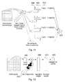
- FIG. 1 is a schematic diagram of a general purpose computer system for use as a face detection system and/or a non-linear editing system.
- the computer system comprises a processing unit 10 having (amongst other conventional components) a central processing unit (CPU) 20, memory such as a random access memory (RAM) 30 and non-volatile storage such as a disc drive 40.
- the computer system may be connected to a network 50 such as a local area network or the Internet (or both).
- a keyboard 60, mouse or other user input device 70 and display screen 80 are also provided.
- a general purpose computer system may include many other conventional parts which need not be described here.
- FIG. 2 is a schematic diagram of a video camera-recorder (camcorder) using face detection.
- the camcorder 100 comprises a lens 110 which focuses an image onto a charge coupled device (CCD) image capture device 120.
- CCD charge coupled device
- the resulting image in electronic form is processed by image processing logic 130 for recording on a recording medium such as a tape cassette 140.
- the images captured by the device 120 are also displayed on a user display 150 which may be viewed through an eyepiece 160.
- one or more microphones are used. These may be external microphones, in the sense that they are connected to the camcorder by a flexible cable, or maybe mounted on the camcorder body itself. Analogue audio signals from the microphone (s) are processed by an audio processing arrangement 170 to produce appropriate audio signals for recording on the storage medium 140.
- the video and audio signals may be recorded on the storage medium 140 in either digital form or analogue form, or even in both forms.
- the image processing arrangement 130 and the audio processing arrangement 170 may include a stage of analogue to digital conversion.
- the camcorder user is able to control aspects of the lens 110's performance by user controls 180 which influence a lens control arrangement 190 to send electrical control signals 200 to the lens 110.
- user controls 180 which influence a lens control arrangement 190 to send electrical control signals 200 to the lens 110.
- attributes such as focus and zoom are controlled in this way, but the lens aperture or other attributes may also be controlled by the user.
- a push button 210 is provided to initiate and stop recording onto the recording medium 140.
- one push of the control 210 may start recording and another push may stop recording, or the control may need to be held in a pushed state for recording to take place, or one push may start recording for a certain timed period, for example five seconds.
- GSM good shot marker
- the metadata may be recorded in some spare capacity (e.g. "user data") on the recording medium 140, depending on the particular format and standard in use.
- the metadata can be stored on a separate storage medium such as a removable MemoryStick RTM memory (not shown), or the metadata could be stored on an external database (not shown), for example being communicated to such a database by a wireless link (not shown).
- the metadata can include not only the GSM information but also shot boundaries, lens attributes, alphanumeric information input by a user (e.g. on a keyboard - not shown), geographical position information from a global positioning system receiver (not shown) and so on.
- the camcorder includes a face detector arrangement 230.
- the face detector arrangement 230 receives images from the image processing arrangement 130 and detects, or attempts to detect, whether such images contain one or more faces.
- the face detector may output face detection data which could be in the form of a "yes/no" flag or maybe more detailed in that the data could include the image co-ordinates of the faces, such as the co-ordinates of eye positions within each detected face. This information may be treated as another type of metadata and stored in any of the other formats described above.
- face detection may be assisted by using other types of metadata within the detection process.
- the face detector 230 receives a control signal from the lens control arrangement 190 to indicate the current focus and zoom settings of the lens 110. These can assist the face detector by giving an initial indication of the expected image size of any faces that may be present in the foreground of the image.
- the focus and zoom settings between them define the expected separation between the camcorder 100 and a person being filmed, and also the magnification of the lens 110. From these two attributes, based upon an average face size, it is possible to calculate the expected size (in pixels) of a face in the resulting image data.
- a conventional (known) speech detector 240 receives audio information from the audio processing arrangement 170 and detects the presence of speech in such audio information.
- the presence of speech may be an indicator that the likelihood of a face being present in the corresponding images is higher than if no speech is detected.
- the speech detector may be modified so as to provide a degree of location of a speaker by detecting a most active microphone from a set of microphones, or by a triangulation or similar technique between multiple microphones.
- the GSM information 220 and shot information are supplied to the face detector 230, to indicate shot boundaries and those shots considered to be most useful by the user.
- ADCs analogue to digital converters
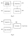
- FIG. 3 is a schematic diagram illustrating a training phase
- Figure 4 is a schematic diagram illustrating a detection phase.
- the present method is based on modelling the face in parts instead of as a whole.
- the parts can either be blocks centred over the assumed positions of the facial features (so-called “selective sampling”) or blocks sampled at regular intervals over the face (so-called “regular sampling”).
- selective sampling blocks centred over the assumed positions of the facial features
- regular sampling blocks sampled at regular intervals over the face
- an analysis process is applied to a set of images known to contain faces, and (optionally) another set of images (“nonface images”) known not to contain faces.
- the analysis process builds a mathematical model of facial and nonfacial features, against which a test image can later be compared (in the detection phase).
- One such histogram is prepared for each possible block position, by repeating the above steps in respect of a large number of test face images.
- the test data are described further in Appendix A below. So, in a system which uses an array of 8 x 8 blocks, 64 histograms are prepared. In a later part of the processing, a test quantised attribute is compared with the histogram data; the fact that a whole histogram is used to model the data means that no assumptions have to be made about whether it follows a parameterised distribution, e.g. Gaussian or otherwise. To save data storage space (if needed), histograms which are similar can be merged so that the same histogram can be reused for different block positions.
- a parameterised distribution e.g. Gaussian or otherwise.
- a set of "nonface” images can be used to generate a corresponding set of “nonface” histograms. Then, to achieve detection of a face, the "probability" produced from the nonface histograms may be compared with a separate threshold, so that the probability has to be under the threshold for the test window to contain a face. Alternatively, the ratio of the face probability to the nonface probability could be compared with a threshold.
- Extra training data may be generated by applying "synthetic variations" 330 to the original training set, such as variations in position, orientation, size, aspect ratio, background scenery, lighting intensity and frequency content.
- eigenblocks are core blocks (or eigenvectors) representing different types of block which may be present in the windowed image.
- eigenblocks are core blocks (or eigenvectors) representing different types of block which may be present in the windowed image.
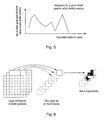
- the generation of eigenblocks will first be described with reference to Figure 6.
- the attributes in the present embodiment are based on so-called eigenblocks.
- the eigenblocks were designed to have good representational ability of the blocks in the training set. Therefore, they were created by performing principal component analysis on a large set of blocks from the training set. This process is shown schematically in Figure 6 and described in more detail in Appendix B.
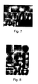
- a second set of eigenblocks was generated from a much larger set of training blocks. These blocks were taken from 500 face images in the training set. In this case, the 16x16 blocks were sampled every 8 pixels and so overlapped by 8 pixels. This generated 49 blocks from each 64x64 training image and led to a total of 24,500 training blocks.
- the first 12 eigenblocks generated from these training blocks are shown in Figure 8.
- Empirical results show that eigenblock set II gives slightly better results than set I. This is because it is calculated from a larger set of training blocks taken from face images, and so is perceived to be better at representing the variations in faces. However, the improvement in performance is not large.
- a histogram was built for each sampled block position within the 64x64 face image.
- the number of histograms depends on the block spacing. For example, for block spacing of 16 pixels, there are 16 possible block positions and thus 16 histograms are used.
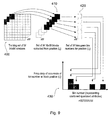
- the process used to build a histogram representing a single block position is shown in Figure 9.
- the histograms are created using a large training set 400 of M face images. For each face image, the process comprises:
- M is very large, e.g. several thousand. This can more easily be achieved by using a training set made up of a set of original faces and several hundred synthetic variations of each original face.
- a histogram bin number is generated from a given block using the following process, as shown in Figure 10.
- the 16 ⁇ 16 block 440 is extracted from the 64x64 window or face image.
- the block is projected onto the set 450 of A eigenblocks to generate a set of "eigenblock weights".
- These eigenblock weights are the "attributes" used in this implementation. They have a range of-1 to +1. This process is described in more detail in Appendix B .
- the bin “contents”, i.e. the frequency of occurrence of the set of attributes giving rise to that bin number, may be considered to be a probability value if it is divided by the number of training images M. However, because the probabilities are compared with a threshold, there is in fact no need to divide through by M as this value would cancel out in the calculations. So, in the following discussions, the bin “contents” will be referred to as "probability values”, and treated as though they are probability values, even though in a strict sense they are in fact frequencies of occurrence.
- the face detection process involves sampling the test image with a moving 64x64 window and calculating a face probability at each window position.
- the calculation of the face probability is shown in Figure 11.
- the block's bin number 490 is calculated as described in the previous section.
- each bin number is looked up and the probability 510 of that bin number is determined.
- the sum 520 of the logs of these probabilities is then calculated across all the blocks to generate a face probability value, P face (otherwise referred to as a log likelihood value).
- This process generates a probability "map" for the entire test image.
- a probability value is derived in respect of each possible window centre position across the image.
- the combination of all of these probability values into a rectangular (or whatever) shaped array is then considered to be a probability "map" corresponding to that image.
- This map is then inverted, so that the process of finding a face involves finding minima in the inverted map (of course this is equivalent to not inverting the map and finding maxima; either could be done).
- a so-called distance-based technique is used. This technique can be summarised as follows: The map (pixel) position with the smallest value in the inverted probability map is chosen. If this value is larger than a threshold (TD), no more faces are chosen. This is the termination criterion. Otherwise a face-sized block corresponding to the chosen centre pixel position is blanked out (i.e. omitted from the following calculations) and the candidate face position finding procedure is repeated on the rest of the image until the termination criterion is reached.
- TD threshold
- the nonface model comprises an additional set of histograms which represent the probability distribution of attributes in nonface images.
- the histograms are created in exactly the same way as for the face model, except that the training images contain examples of nonfaces instead of faces.
- P combined is then used instead of P face to produce the probability map (before inversion).
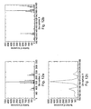
- Figures 12a to 12f show some examples of histograms generated by the training process described above.
- Figures 12a, 12b and 12c are derived from a training set of face images
- Figures 12d, 12e and 12f are derived from a training set of nonface images.
- Figures 12a, 12b and 12c are derived from a training set of face images
- Figures 12d, 12e and 12f are derived from a training set of nonface images.
- the histograms store statistical information about the likelihood of a face at a given scale and location in an image.
- the ordering of the histograms is unexpectedly significant to system performance.
- a simple ordering can result in the access being non-localised (i.e. consecutive accesses are usually far apart in memory). This can give poor cache performance when implemented using microprocessors or bespoke processors.
- the histograms are reordered so that the access to the data are more localised.
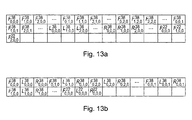
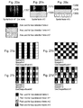
- F 38 Frontal face with an eye spacing of 38 pixels that is, a "zoomed in” histogram) L 38 Face facing to the left by 25 degrees, with an eye spacing of 38 pixels R 38 Face facing to the right by 25 degrees, with an eye spacing of 38 pixels
- F 22 Frontal face with an eye spacing of 22 pixels that is, a "full face” histogram) L 22 Face facing to the left by 25 degrees, with an eye spacing of 22 pixels R 22 Face facing to the right by 25 degrees, with an eye spacing of 22 pixels
- F 38 / c,x,y is the value of the histogram for a given c,x & y.
- F 38 / 15,4,5 is the value given by the frontal histogram with the 38 eye spacing at location (4,5) in the face window, for a binmap value of 15.
- a straightforward ordering of the histograms in memory is by c , then x , then y , then pose, and then eye spacing.
- a schematic example of this ordering is shown in Figure 13a.
- An improved ordering system is by pose then x then y then c and then eye spacing.
- a schematic example of this type of ordering is shown in Figure 13b.
- the three different poses are always accessed with the same bin-number and location for each location. i.e. if F 38 / 329,2,1 is accessed, then L 38 / 329,2,1 & R 38 / 329,2,1 are also accessed. These are adjacent in the new method, so excellent cache performance is achieved.
- the new method of organising the histograms also takes advantage of the way that the face window moves during a search for faces in the image. Because of the way that the face window moves the same c value will be looked up in many ( x , y ) locations.
- Figure 14 shows which values are used from the bin map to look for a face in a certain location.
- F 38 / 329,2,1 is the value from the frontal histogram for eye spacing 38 for the (2,1) location in the face window.
- the values stored in each histogram bin are quantised to a different number of bits depending on which pose they represent.
- each set of 3 histogram values can be stored in 2 bytes instead of 3.
- the test image is scaled by a range of factors and a distance (i.e. probability) map is produced for each scale.
- a distance map is produced for each scale.
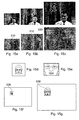
- FIGs 15a to 15c the images and their corresponding distance maps are shown at three different scales.
- the method gives the best response (highest probability, or minimum distance) for the large (central) subject at the smallest scale (Fig 15a) and better responses for the smaller subject (to the left of the main figure) at the larger scales. (A darker colour on the map represents a lower value in the inverted map, or in other words a higher probability of there being a face).
- Candidate face positions are extracted across different scales by first finding the position which gives the best response over all scales.
- the highest probability (lowest distance) is established amongst all of the probability maps at all of the scales.
- This candidate position is the first to be labelled as a face.
- the window centred over that face position is then blanked out from the probability map at each scale.
- the size of the window blanked out is proportional to the scale of the probability map.
- FIGS 15a to 15c Examples of this scaled blanking-out process are shown in Figures 15a to 15c.
- the highest probability across all the maps is found at the left hand side of the largest scale map ( Figure 15c).
- An area 530 corresponding to the presumed size of a face is blanked off in Figure 15c.
- Corresponding, but scaled, areas 532, 534 are blanked off in the smaller maps.
- Areas larger than the test window may be blanked off in the maps, to avoid overlapping detections.
- an area equal to the size of the test window surrounded by a border half as wide/long as the test window is appropriate to avoid such overlapping detections.
- the intervals allowed between the scales processed are influenced by the sensitivity of the method to variations in size. It was found in this preliminary study of scale invariance that the method is not excessively sensitive to variations in size as faces which gave a good response at a certain scale often gave a good response at adjacent scales as well.
- the above description refers to detecting a face even though the size of the face in the image is not known at the start of the detection process.
- Another aspect of multiple scale face detection is the use of two or more parallel detections at different scales to validate the detection process. This can have advantages if, for example, the face to be detected is partially obscured, or the person is wearing a hat etc.
- Figures 15d to 15g schematically illustrate this process.
- the system is trained on windows (divided into respective blocks as described above) which surround the whole of the test face (Figure 15d) to generate "full face” histogram data and also on windows at an expanded scale so that only a central area of the test face is included ( Figure 15e) to generate "zoomed in” histogram data.
- This generates two sets of histogram data. One set relates to the "full face” windows of Figure 15d, and the other relates to the "central face area" windows of Figure 15e.
- the window is applied to two different scalings of the test image so that in one (Figure 15f) the test window surrounds the whole of the expected size of a face, and in the other ( Figure 15g) the test window encompasses the central area of a face at that expected size.
- Figure 15f the test window surrounds the whole of the expected size of a face
- Figure 15g the test window encompasses the central area of a face at that expected size.
- the multiple scales for the arrangements of Figures 15a to 15c are arranged in a geometric sequence.
- each scale in the sequence is a factor of different to the adjacent scale in the sequence.
- the larger scale, central area, detection is carried out at a scale 3 steps higher in the sequence, that is, 23 ⁇ 4 times larger than the "full face" scale, using attribute data relating to the scale 3 steps higher in the sequence.
- the geometric progression means that the parallel detection of Figures 15d to 15g can always be carried out using attribute data generated in respect of another multiple scale three steps higher in the sequence.
- the two processes can be combined in various ways.
- the multiple scale detection process of Figures 15a to 15c can be applied first, and then the parallel scale detection process of Figures 15d to 15g can be applied at areas (and scales) identified during the multiple scale detection process.
- a convenient and efficient use of the attribute data may be achieved by:
- Further parallel testing can be performed to detect different poses, such as looking straight ahead, looking partly up, down, left, right etc.
- a respective set of histogram data is required and the results are preferably combined using a "max" function, that is, the pose giving the highest probability is carried forward to thresholding, the others being discarded.
- the face detection algorithm provides many probability maps at many scales; the requirement is to find all the places in the image where the probability exceeds a given threshold, whilst ensuring that there are no overlapping faces.
- a disadvantage of the method described above is that it requires the storage of a complete set of probability maps at all scales, which is a large memory requirement.
- the following technique does not require the storage of all of the probability maps simultaneously.
- a temporary list of candidate face locations is maintained. As the probability map for each scale is calculated, the probability maxima are found and compared against the list of candidate face locations to ensure that no overlapping faces exist.
- this method uses a face list to maintain a list of current locations when there might be a face.
- Each face in the face list has a face location and a face size.
- the threshold is the probability threshold above which an object is deemed to be a face.
- the scale factor is the size factor between successive scales (1.189207115 or in the present embodiment).
- a 16 x 16 face_size is considered in the example description below.
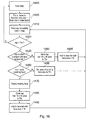
- the process starts at a step 1400 in respect of one of the scales (in the example shown, the smallest scale).
- the face list will be empty, but in general, for all faces in the face list, the face size for each face is modified at the step 1400 by multiplying the respective face size by the scale factor. This makes sure that faces detected in respect of the previous scale are correctly sized for a valid comparison with any maxima in the current scale.
- the maximum probability value, mp is detected in the current map.
- the maximum probability value mp is compared with the threshold. If mp is greater than the threshold then control passes to a step 1430. On the other hand, if mp is not greater than the threshold then processing of the next map (corresponding to the next scale factor to be dealt with) is initiated at a step 1440.
- the value mp is compared with a stored probability value in respect of the existing face. If mp is greater than that probability then the existing face is deleted at a step 1470 and a new entry created in the face list corresponding to the current value and position of mp. In particular, the value mp is stored in respect of the new entry in the face list and a 16x16 pixel area centred on the image position of the current maximum probability is set to the threshold at a step 1480. At a step 1490 the current location of the maximum probability value is added to the face list with a face size of 16. Control then returns to the step 1410.
- step 1460 if the maximum probability location was detected not to overlap with any faces in the face list (at the step 1430) then a new entry is created in the face list.
- the value mp is stored and a 16 ⁇ 16 area surrounding the current maximum value is set to the threshold.
- the current maximum position is added to the face list with a face size of 16 and control returns to the step 1410.
- a maximum probability value mp is again detected, but this will be in the light of modifications to the probability values surrounding detected faces in the steps 1460, 1455 and 1480. So, the modified values created at those steps will not in fact pass the test of the step 1420, in that a value set to equal the threshold value will be found not to exceed it. Accordingly, the step 1420 will establish whether another position exists in the correct map where the threshold value is exceeded.
- An advantage of this method is that it allows each scale of probability map to be considered separately. Only the face list needs to be stored in between processing each scale. This has the following advantages:
- a change detection process is used to detect which areas of the image have changed since the previous frame, or at least to remove from the face detection process certain areas detected not to have changed since the previous frame.
- Areas of the image that have not changed since the previous frame do not need to have face detection performed on them again, as the result is likely to be the same as the previous frame. However, areas of the images that have changed need to have face detection performed on them afresh. These areas of the image are labelled as "areas of interest" during change detection.
- change detection is performed only at a single fixed scale, e.g. the original image scale or the largest scale that is used in face detection.
- a single fixed scale e.g. the original image scale or the largest scale that is used in face detection.
- Figure 17 which schematically illustrates a motion detector.
- the current and previous frames are first processed by low pass filters 1100, 1110.
- the two frames are then supplied to a differencer 1120 to produce a frame difference image, for example a representation of the absolute pixel (or block) differences between frames with one difference value per pixel (or block) position.
- the absolute values of the difference image are then thresholded 1130 by comparison with a threshold value Thr diff to create a binary difference image, i.e. an array of one-bit values with one value per pixel (or block) position: very small differences are set to zero (no change) and larger differences are set to one (change detected).
- a morphological opening operation is performed 1140 on the binary difference image to create more contiguous areas of detected change/motion.
- the low-pass filtering operation may be omitted.
- Morphological opening is a known image processing technique and in this example is performed on a 3x3 area (i.e. a 3x3 block is used as the morphological structuring element) and comprises a morphological erosion operation followed by a morphological dilation operation.
- the morphological processing is carried out after processing every third line.
- Change detection can be applied to the whole image, as described above, to create a map of areas of the image where changes have been detected. Face detection is applied to those areas.
- change detection can be used to eliminate certain areas of the image from face detection, though without necessarily detecting all areas of motion or "no motion". This technique has the advantage of reducing the processing requirements of the change detection process while still potentially providing a useful saving in processing for the face detection itself.
- a schematic example of this process is illustrated in Figures 18a to 18e.
- the scan 1150 progresses until the detected absolute difference in respect of one scan position 1160 exceeds the threshold Thr diff . At this point the scan 1150 terminates.
- the scan 1170 is a horizontal scan starting at the bottom of the image and terminates when a scan position 1200 gives rise to an absolute difference value exceeding the threshold Thr diff .
- the scan 1180 is a downwards vertical scan starting at the left hand side of the image and terminates when a scan position 1210 gives rise to an absolute difference value exceeding the threshold Thr diff .
- the scan 1190 is a downwards vertical scan starting at the right hand side of the image and terminates when a scan position 1220 gives rise to an absolute difference value exceeding the threshold Thr diff .
- the four points 1160, 1200, 1210, 1220 define a bounding box 1230 in Figure 18e.
- the four vertices of the bounding box 1230 are given by: top left (x 1210, y 1160 ) top right (x 1220, y 1160 ) bottom left (x 1210 , y 1200 ) bottom right (x 1220 , y 1200 )
- the bounding box therefore does not define all areas of the image in which changes have been detected, but instead it defines an area (outside the bounding box) which can be excluded from face processing because change has not been detected there.
- an area outside the bounding box
- the area inside the bounding box potentially all of the area may have changed, but a more usual situation would be that some parts of that area may have changed and some not.
- the two vertical scans 1180', 1190' are carried out only in respect of those rows 1240 which have not already been eliminated by the two horizontal scans 1150, 1170. This variation can reduce the processing requirements.
- change detection is carried out, starting from four extremes (edges) of the image, and stops in each case when a change is detected. So, apart from potentially the final pixel (or block) or part row/column of each of the change detection processes, change detection is carried out only in respect of those image areas which are not going to be subject to face detection. Similarly, apart from that final pixel, block or part row/column, face detection is carried out only in respect of areas which have not been subject to the change detection process. Bearing in mind that change detection is less processor-intensive than face detection, this relatively tiny overlap between the two processes means that in almost all situations the use of change detection will reduce the overall processing requirements of an image.
- a different method of change detection applies to motion-encoded signals such as MPEG-encoded signals, or those which have been previously encoded in this form and decoded for face detection.
- Motion vectors or the like associated with the signals can indicate where an inter-image change has taken place.
- a block (e.g. an MPEG macroblock) at the destination (in a current image) of each motion vector can be flagged as an area of change. This can be done instead of or in addition to the change detection techniques described above.
- Another method of reducing the processing requirements is as follows.
- the face detection algorithm is divided into a number of stages that are repeated over many scales.
- the algorithm is only completed after n calls.
- the algorithm is automatically partitioned so that each call takes approximately an equal amount of time.
- the key features of this method are:
- Process Scale Description Motion 1 Motion is used to reduce search area Variance 1 Image variance is used to reduce search area Decimate 1 ⁇ 2 Image is reduced in size to next scale Convolve 2 Image is convolved to produce bin-map Decimate 2 ⁇ 3 Convolve 3 Decimate 3 ⁇ 4 Convolve 4 Lookup 4 Bin-maps are used to lookup face probabilities Max-Search 4 Maximum probabilities are found and thresholded Decimate 4 ⁇ 5 Convolve 5 Lookup 5 Max-Search 5 Decimate 5 ⁇ 6 Convolve 6 Lookup 6 Max-Search 6 Tracking -
- the following table shows what might happen if a temporal decimation of 4 is used.
- the algorithm automatically divides up the processing into 'chunks' of equal time - this is complicated by the fact that the processing for the earlier scales requires more time than the processing for later scales (the images being larger for the earlier scales).
- the algorithm estimates the amount of time that each stage will require before carrying it out. This estimate is given by the particular process and the number of pixels to be processed for a given scale.
- the system calculates whether the number of cumulated processing units required will take it over some prearranged level (5300 for example). If it does, then a return is carried out without executing this stage. This has the advantage over timing that it is known in advance of doing something whether it will exceed the allotted time.
- Horizontal striping was chosen because it is considered more efficient to process horizontal stripes, although any sort of division could be used (squares, vertical stripes etc.)
- Figures 20a to 20c schematically illustrate a striping technique.
- no spatial decimation is used and the entire image 1300 is subjected to face detection.
- the image is split into two portions 1310, 1320. These are each subjected to face detection in alternate images.
- the image is split into three portions 1330, 1340, 1350 so that each portion is subjected to face detection for one in every three images. The portions may be distinct or may overlap slightly.
- FIGS 21a to 12d schematically illustrate so-called sparse spatial decimation.
- Figure 21a to 21d are as follows: Figure 21a Figure 21b Figure 21c Figure 21d SparseX 2 2 2 2 SparseY 1 1 2 2 UseChequerBoard 0 1 0 1
- a combination of spatial and temporal decimation can be used. For example, discrete spatial portions of an image (e.g. a third of an image) could be processed over a number of frames. The portions (e.g. the three thirds) processed in this way could come from the same image or from different respective images.
- the tracking algorithm aims to improve face detection performance in image sequences.
- the initial aim of the tracking algorithm is to detect every face in every frame of an image sequence. However, it is recognised that sometimes a face in the sequence may not be detected. In these circumstances, the tracking algorithm may assist in interpolating across the missing face detections.
- the goal of face tracking is to be able to output some useful metadata from each set of frames belonging to the same scene in an image sequence. This might include:
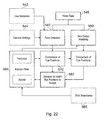
- the tracking algorithm uses the results of the face detection algorithm, run independently on each frame of the image sequence, as its starting point. Because the face detection algorithm may sometimes miss (not detect) faces, some method of interpolating the missing faces is useful. To this end, a Kalman filter was used to predict the next position of the face and a skin colour matching algorithm was used to aid tracking of faces. In addition, because the face detection algorithm often gives rise to false acceptances, some method of rejecting these is also useful.
- input video data 545 (representing the image sequence) is supplied to a face detector of the type described in this application, and a skin colour matching detector 550.
- the face detector attempts to detect one or more faces in each image.
- a Kalman filter 560 is established to track the position of that face.
- the Kalman filter generates a predicted position for the same face in the next image in the sequence.
- An eye position comparator 570, 580 detects whether the face detector 540 detects a face at that position (or within a certain threshold distance of that position) in the next image. If this is found to be the case, then that detected face position is used to update the Kalman filter and the process continues.
- a skin colour matching method 550 is used. This is a less precise face detection technique which is set up to have a lower threshold of acceptance than the face detector 540, so that it is possible for the skin colour matching technique to detect (what it considers to be) a face even when the face detector cannot make a positive detection at that position. If a "face" is detected by skin colour matching, its position is passed to the Kalman filter as an updated position and the process continues.
- the predicted position is used to update the Kalman filter.
- a separate Kalman filter is used to track each face in the tracking algorithm.
- a state model representing the face In order to use a Kalman filter to track a face, a state model representing the face must be created.
- the position of each face is represented by a 4-dimensional vector containing the co-ordinates of the left and right eyes, which in turn are derived by a predetermined relationship to the centre position of the window and the scale being used: where k is the frame number.
- the current state of the face is represented by its position, velocity and acceleration, in a 12-dimensional vector:
- the tracking algorithm does nothing until it receives a frame with a face detection result indicating that there is a face present.
- a Kalman filter is then initialised for each detected face in this frame. Its state is initialised with the position of the face, and with zero velocity and acceleration:
- the state model error covariance, Q and the observation error covariance, R are also assigned some other attributes: the state model error covariance, Q and the observation error covariance, R.
- the error covariance of the Kalman filter, P is also initialised. These parameters are described in more detail below. At the beginning of the following frame, and every subsequent frame, a Kalman filter prediction process is carried out.
- the filter uses the previous state (at frame k-1) and some other internal and external variables to estimate the current state of the filter (at frame k).
- State prediction equation: z b ( k ) ⁇ ( k , k - 1) z a ( k - 1)
- Covariance prediction equation: P b ( k ) ⁇ ( k,k - 1) P a ( k - 1) ⁇ ( k, k -1) T + Q ( k )
- z and b ( k ) denotes the state before updating the filter for frame k
- z and a ( k - 1) denotes the state a fter updating the filter for frame k -1 (or the initialised state if it is a new filter)
- ⁇ ( k,k - 1) is the state transition matrix.
- P b ( k ) denotes the filter's error covariance b efore updating the filter for frame k
- P a ( k - 1) denotes the filter's error covariance a fter updating the filter for the previous frame (or the initialised value if it is a new filter).
- P b ( k ) can be thought of as an internal variable in the filter that models its accuracy.
- Q ( k ) is the error covariance of the state model.
- a high value of Q ( k ) means that the predicted values of the filter's state (i.e. the face's position) will be assumed to have a high level of error. By tuning this parameter, the behaviour of the filter can be changed and potentially improved for face detection.
- the state transition matrix, ⁇ ( k,k - 1) determines how the prediction of the next state is made. Using the equations for motion, the following matrix can be derived for ⁇ ( k,k - 1): where O 4 is a 4x4 zero matrix and I 4 is a 4x4 identity matrix. ⁇ t can simply be set to 1 (i.e. units of t are frame periods).
- This state transition matrix models position, velocity and acceleration. However, it was found that the use of acceleration tended to make the face predictions accelerate towards the edge of the picture when no face detections were available to correct the predicted state. Therefore, a simpler state transition matrix without using acceleration was preferred:
- the predicted eye positions of each Kalman filter, z and b ( k ), are compared to all face detection results in the current frame (if there are any). If the distance between the eye positions is below a given threshold, then the face detection can be assumed to belong to the same face as that being modelled by the Kalman filter.
- the face detection result is then treated as an observation, y ( k ), of the face's current state: where p ( k ) is the position of the eyes in the face detection result. This observation is used during the Kalman filter update stage to help correct the prediction.
- Skin colour matching is not used for faces that successfully match face detection results. Skin colour matching is only performed for faces whose position has been predicted by the Kalman filter but have no matching face detection result in the current frame, and therefore no observation data to help update the Kalman filter.
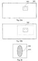
- an elliptical area centred on the face's previous position is extracted from the previous frame.
- An example of such an area 600 within the face window 610 is shown schematically in Figure 24.
- a colour model is seeded using the chrominance data from this area to produce an estimate of the mean and covariance of the Cr and Cb values, based on a Gaussian model.
- Figures 23a and 23b schematically illustrate the generation of the search area.
- Figure 23a schematically illustrates the predicted position 620 of a face within the next image 630.
- a search area 640 surrounding the predicted position 620 in the next image is searched for the face.
- the skin colour matching methods described above use a simple Gaussian skin colour model.
- the model is seeded on an elliptical area centred on the face in the previous frame, and used to find the best matching elliptical area in the current frame.
- two further methods were developed: a colour histogram method and a colour mask method. These will now be described.
- a histogram of Cr and Cb values within a square window around the face is computed. To do this, for each pixel the Cr and Cb values are first combined into a single value. A histogram is then computed that measures the frequency of occurrence of these values in the whole window. Because the number of combined Cr and Cb values is large (256x256 possible combinations), the values are quantised before the histogram is calculated.
- the histogram is used in the current frame to try to estimate the most likely new position of the face by finding the area of the image with the most similar colour distribution. As shown schematically in Figures 23a and 23b, this is done by calculating a histogram in exactly the same way for a range of window positions within a search area of the current frame. This search area covers a given area around the predicted face position. The histograms are then compared by calculating the mean squared error (MSE) between the original histogram for the tracked face in the previous frame and each histogram in the current frame. The estimated position of the face in the current frame is given by the position of the minimum MSE.
- MSE mean squared error
- This method is based on the method first described above. It uses a Gaussian skin colour model to describe the distribution of pixels in the face.
- an elliptical area centred on the face is used to colour match faces, as this may be perceived to reduce or minimise the quantity of background pixels which might degrade the model.
- a similar elliptical area is still used to seed a colour model on the original tracked face in the previous frame, for example by applying the mean and covariance of RGB or YCrCb to set parameters of a Gaussian model (or alternatively, a default colour model such as a Gaussian model can be used, see below).
- a mask area is calculated based on the distribution of pixels in the original face window from the previous frame. The mask is calculated by finding the 50% of pixels in the window which best match the colour model.
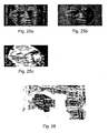
- Figures 25a to 25c An example is shown in Figures 25a to 25c.
- Figure 25a schematically illustrates the initial window under test
- Figure 25b schematically illustrates the elliptical window used to seed the colour model
- Figure 25c schematically illustrates the mask defined by the 50% of pixels which most closely match the colour model.
- a search area around the predicted face position is searched (as before) and the "distance" from the colour model is calculated for each pixel.
- the "distance” refers to a difference from the mean, normalised in each dimension by the variance in that dimension.
- An example of the resultant distance image is shown in Figure 26.
- the pixels of the distance image are averaged over a mask-shaped area. The position with the lowest averaged distance is then selected as the best estimate for the position of the face in this frame.
- This method thus differs from the original method in that a mask-shaped area is used in the distance image, instead of an elliptical area. This allows the colour match method to use both colour and shape information.
- Gaussian skin colour models will now be described further.
- a Gaussian model for the skin colour class is built using the chrominance components of the YCbCr colour space.
- the similarity of test pixels to the skin colour class can then be measured.
- This method thus provides a skin colour likelihood estimate for each pixel, independently of the eigenface-based approaches.
- w be the vector of the CbCr values of a test pixel.
- the probability of w belonging to the skin colour class S is modelled by a two-dimensional Gaussian: where the mean ⁇ s and the covariance matrix ⁇ s of the distribution are (previously) estimated from a training set of skin colour values.
- Skin colour detection is not considered to be an effective face detector when used on its own. This is because there can be many areas of an image that are similar to skin colour but are not necessarily faces, for example other parts of the body. However, it can be used to improve the performance of the eigenblock-based approaches by using a combined approach as described in respect of the present face tracking system.
- the decisions made on whether to accept the face detected eye positions or the colour matched eye positions as the observation for the Kalman filter, or whether no observation was accepted, are stored. These are used later to assess the ongoing validity of the faces modelled by each Kalman filter.
- the update step is used to determine an appropriate output of the filter for the current frame, based on the state prediction and the observation data. It also updates the internal variables of the filter based on the error between the predicted state and the observed state.
- Kalman gain equation State update equation z a ( k ) z b ( k ) + K ( k )[ y ( k ) - H ( k ) z b ( k )]
- Covariance update equation P a ( k ) P b ( k ) - K ( k ) H ( k ) P b ( k )
- K ( k ) denotes the Kalman gain, another variable internal to the Kalman filter. It is used to determine how much the predicted state should be adjusted based on the observed state, y ( k ) .
- H ( k ) is the observation matrix. It determines which parts of the state can be observed. In our case, only the position of the face can be observed, not its velocity or acceleration, so the following matrix is used for H ( k ) :
- R ( k ) is the error covariance of the observation data.
- a high value of R ( k ) means that the observed values of the filter's state (i.e. the face detection results or colour matches) will be assumed to have a high level of error.
- the behaviour of the filter can be changed and potentially improved for face detection.
- a large value of R ( k ) relative to Q ( k ) was found to be suitable (this means that the predicted face positions are treated as more reliable than the observations). Note that it is permissible to vary these parameters from frame to frame. Therefore, an interesting future area of investigation may be to adjust the relative values of R ( k ) and Q ( k ) depending on whether the observation is based on a face detection result (reliable) or a colour match (less reliable).
- the updated state, z and a ( k ) is used as the final decision on the position of the face. This data is output to file and stored.
- the associated Kalman filter is removed and no data is output to file.
- the tracking results up to the frame before it leaves the picture may be stored and treated as valid face tracking results (providing that the results meet any other criteria applied to validate tracking results).
- the tracking process is not limited to tracking through a video sequence in a forward temporal direction. Assuming that the image data remain accessible (i.e. the process is not real-time, or the image data are buffered for temporary continued use), the entire tracking process could be carried out in a reverse temporal direction. Or, when a first face detection is made (often part-way through a video sequence) the tracking process could be initiated in both temporal directions. As a further option, the tracking process could be run in both temporal directions through a video sequence, with the results being combined so that (for example) a tracked face meeting the acceptance criteria is included as a valid result whichever direction the tracking took place.
- a face track is started for every face detection that cannot be matched up with an existing track. This could lead to many false detections being erroneously tracked and persisting for several frames before finally being rejected by one of the existing rules (e.g. prediction_acceptance_ratio_threshold)
- the rules for rejecting a track e.g. prediction_ acceptance_ ratio _threshold, detection _acceptance_ ratio_ threshold
- prediction_ acceptance_ ratio _threshold e.g. prediction_ acceptance_ ratio _threshold, detection _acceptance_ ratio_ threshold
- the first part of the solution helps to prevent false detections from setting off erroneous tracks.
- a face track is still started internally for every face detection that does not match an existing track. However, it is not output from the algorithm.
- the first f frames in the track must be face detections (i.e. of type D ). If all of the first f frames are of type D then the track is maintained and face locations are output from the algorithm from frame f onwards. If all of the first n frames are not of type D , then the face track is terminated and no face locations are output for this track.
- f is typically set to 2, 3 or 5.
- the second part of the solution allows faces in profile to be tracked for a long period, rather than having their tracks terminated due to a low detection_ acceptance _ratio prediction_ acceptance_ ratio_ threshold and detection_ acceptance_ ratio _threshold are not turned on in this case. Instead, an option is to include the following criterion to maintain a face track:
- the skin colour of the face is only checked during skin colour tracking. This means that non-skin-coloured false detections may be tracked, or the face track may wander off into non-skin-coloured locations by using the predicted face position.
- An efficient way to implement this is to use the distance from skin colour of each pixel calculated during skin colour tracking. If, this measure averaged over the face area (either over a mask shaped area, over an elliptical area or over the whole face window depending on which skin colour tracking method is being used), exceeds a fixed threshold, then the face track is terminated.
- an area of interest pre-processor is used to ascertain which areas of the image have non-face-like variance. This is repeated at every scale, and these areas are then omitted from face detection processing. However, it is still possible for a skin colour tracked or Kalman predicted face to move into a (non-face-like) low or high variance area of the image.
- the variance values (or gradient values) for the areas around existing face tracks are stored.
- the position is validated against the stored variance (or gradient) values in the area of interest map. If the position is found to have very high or very low variance (or gradient), it is considered to be non-face-like and the face track is terminated. This avoids face tracks wandering onto low (or high) variance background areas of the image. Alternatively, the variance of the new face position is calculated afresh (useful if variance-pre-processing is not used).
- variance measure used can either be traditional variance or the sum of differences of neighbouring pixels (gradient) or any other variance-type measure.
- Shot boundary data 560 (from metadata associated with the image sequence under test; or metadata generated within the camera of Figure 2) defines the limits of each contiguous "shot” within the image sequence.
- the Kalman filter is reset at shot boundaries, and is not allowed to carry a prediction over to a subsequent shot, as the prediction would be meaningless.
- User metadata 542 and camera setting metadata 544 are supplied as inputs to the face detector 540. These may also be used in a non-tracking system. Examples of the camera setting metadata were described above.
- User metadata may include information such as:
- the type of programme is relevant to the type of face which may be expected in the images or image sequence. For example, in a news programme, one would expect to see a single face for much of the image sequence, occupying an area of (say) 10% of the screen.
- the detection of faces at different scales can be weighted in response to this data, so that faces of about this size are given an enhanced probability.
- Another alternative or additional approach is that the search range is reduced, so that instead of searching for faces at all possible scales, only a subset of scales is searched. This can reduce the processing requirements of the face detection process.
- the software can run more quickly and/or on a less powerful processor.
- a hardware-based system including for example an application-specific integrated circuit (ASIC) or field programmable gate array (FPGA) system
- the hardware needs may be reduced.
- the other types of user metadata mentioned above may also be applied in this way.
- the "expected face size" sub-ranges may be stored in a look-up table held in the memory 30, for example.
- camera metadata for example the current focus and zoom settings of the lens 110
- these can also assist the face detector by giving an initial indication of the expected image size of any faces that may be present in the foreground of the image.
- the focus and zoom settings between them define the expected separation between the camcorder 100 and a person being filmed, and also the magnification of the lens 110. From these two attributes, based upon an average face size, it is possible to calculate the expected size (in pixels) of a face in the resulting image data, leading again to a sub-range of sizes for search or a weighting of the expected face sizes.
- the face tracking technique has three main benefits:
- the skin colour tracking technique described earlier worked by matching the colour distance mask of the face in the previous frame to the colour distance map of the current frame.
- This method which at least some of the variations aim to improve:
- Variation 6 in which the colour distance mask for the face is only slowly updated, addresses aspects (i) and (ii). As well as getting a good match for skin colour areas within the facemask, non face coloured areas are also considered in Variation 5, which addresses (iii).
- a binary mask is calculated from the previous frame's colour distance map at the location of the face within this frame.
- Each element of the mask is either ' 1' if it is less than the average colour distance value for the entire mask (i.e. it is skin coloured), or else '0' (non-skin-coloured).
- a search is conducted over the search window using the binary mask. At each point within the search window, a value is calculated by summing all the colour distance values where the mask is '1' and subtracting all the colour distance values where the mask is '0'. The best match is taken to be the position at which the mask gives the minimum summed colour distance value.
- the current colour distance map (for frame n ) is updated by summing 90% of the old colour distance map at the old face location 1500 with 10% of the new colour distance map at the new face location 1510.
- searching takes place over a 4x4 grid (i.e. the searching cannot be more accurate than 4 pixels), using the earlier method. If the face moves 1 pixel the searching algorithm will find the face in the same (previous) location. Since the colour distance map was completely replaced with the new one, if the face continues to move at 1 pixel a frame, after 4 frames the face will still be found in the original location, even though it should have now moved 4 pixels - in other words, the mask has 'slipped' from the face.
- each pixel in the map is set to -1 if it is below the average colour distance value of the mask and to +1 if it is above the average colour distance value of the mask (the "average colour distance of the mask” refers to the average colour distance of the face window before it was quantised to '1's and '0's to form the mask).
- a value is calculated at each point within the search window by summing all the colour distance values where the mask is '1' and subtracting all the colour distance values where the mask is '0'.
- these values are calculated and summed for a face-sized window.
- the best match is taken as the pixel location where the minimum value is obtained, i.e. where the mask best matches the image.
- This method prevents the magnitude of the colour distance values from having an undue effect on the distance from skin colour calculation so that very non-skin coloured pixels outside the mask do not have undue influence.
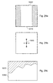
- Figures 29a to 29c schematically illustrate a gradient pre-processing technique.
- a pre-processing step is proposed to remove areas of little pixel variation from the face detection process.
- the pre-processing step can be carried out at each scale.
- the basic process is that a "gradient test" is applied to each possible window position across the whole image.
- a predetermined pixel position for each window position such as the pixel at or nearest the centre of that window position, is flagged or labelled in dependence on the results of the test applied to that window. If the test shows that a window has little pixel variation, that window position is not used in the face detection process.
- FIG 29a A first step is illustrated in Figure 29a. This shows a window at an arbitrary window position in the image. As mentioned above, the pre-processing is repeated at each possible window position. Referring to Figure 29a, although the gradient pre-processing could be applied to the whole window, it has been found that better results are obtained if the pre-processing is applied to a central area 1000 of the test window 1010.
- a gradient-based measure is derived from the window (or from the central area of the window as shown in Figure 29a), which is the average of the absolute differences between all adjacent pixels 1011 in both the horizontal and vertical directions, taken over the window.
- Each window centre position is labelled with this gradient-based measure to produce a gradient "map" of the image.
- the resulting gradient map is then compared with a threshold gradient value. Any window positions for which the gradient-based measure lies below the threshold gradient value are excluded from the face detection process in respect of that image.
- the gradient-based measure is preferably carried out in respect of pixel luminance values, but could of course be applied to other image components of a colour image.
- Figure 29c schematically illustrates a gradient map derived from an example image.
- a lower gradient area 1070 (shown shaded) is excluded from face detection, and only a higher gradient area 1080 is used.
- the embodiments described above have related to a face detection system (involving training and detection phases) and possible uses for it in a camera-recorder and an editing system. It will be appreciated that there are many other possible uses of such techniques, for example (and not limited to) security surveillance systems, media handling in general (such as video tape recorder controllers), video conferencing systems, IP cameras, digital stills cameras and the like.
- window positions having high pixel differences can also be flagged or labelled, and are also excluded from the face detection process.
- a "high" pixel difference means that the measure described above with respect to Figure 29b exceeds an upper threshold value.
- a gradient map is produced as described above. Any positions for which the gradient measure is lower than the (first) threshold gradient value mentioned earlier are excluded from face detection processing, as are any positions for which the gradient measure is higher than the upper threshold value.
- the "lower threshold” processing is preferably applied to a central part 1000 of the test window 1010.
- the same can apply to the "upper threshold” processing. This would mean that only a single gradient measure needs to be derived in respect of each window position.
- the whole window is used in respect of the lower threshold test, the whole window can similarly be used in respect of the upper threshold test. Again, only a single gradient measure needs to be derived for each window position.
- a further criterion for rejecting a face track is that its variance or gradient measure is very low or very high.
- the position is validated against the stored variance (or gradient) values in the area of interest map. If the position is found to have very high or very low variance (or gradient), it is considered to be non-face-like and the face track is terminated. This prevents face tracks from wandering onto low (or high) variance background areas of the image.
- the variance of the new face position can be calculated afresh.
- the variance measure used can either be traditional variance or the sum of differences of neighbouring pixels (gradient) or any other variance-type measure.
- one or more rectangular bounding boxes are placed around the areas of detected motion (or at least, so as to exclude areas which have no detected motion). These boxes are then rescaled to all the scales at which face detection is to be carried out.
- the area of interest decision which is to say a decision as to which areas are to be subjected to face detection, is based on the outputs from the variance pre-processing and change detection processes.
- the area of interest decision logic combines the areas of interest from the variance pre-processing and change detection modules to produce a final area of interest. These are constrained by one or more rectangular bounding boxes at each scale or (without limitation to bounding boxes) a multi-scale "area of interest" map, with each pixel position being labelled as an area of interest or not.
Applications Claiming Priority (2)
| Application Number | Priority Date | Filing Date | Title |
|---|---|---|---|
| GB0328739A GB2409029A (en) | 2003-12-11 | 2003-12-11 | Face detection |
| GB0328739 | 2003-12-11 |
Publications (2)
| Publication Number | Publication Date |
|---|---|
| EP1542154A2 true EP1542154A2 (fr) | 2005-06-15 |
| EP1542154A3 EP1542154A3 (fr) | 2006-05-17 |
Family
ID=30130048
Family Applications (1)
| Application Number | Title | Priority Date | Filing Date |
|---|---|---|---|
| EP04256854A Withdrawn EP1542154A3 (fr) | 2003-12-11 | 2004-11-05 | Détection d'objets |
Country Status (3)
| Country | Link |
|---|---|
| US (1) | US20050128306A1 (fr) |
| EP (1) | EP1542154A3 (fr) |
| GB (1) | GB2409029A (fr) |
Cited By (10)
| Publication number | Priority date | Publication date | Assignee | Title |
|---|---|---|---|---|
| WO2007042044A1 (fr) * | 2005-10-14 | 2007-04-19 | Unisense Fertilitech A/S | Determination d'un changement dans une population cellulaire |
| WO2008012631A1 (fr) | 2006-07-27 | 2008-01-31 | Videotec S.P.A. | Procédé de détection d'événements et système de surveillance vidéo utilisant ledit procédé |
| RU2466456C2 (ru) * | 2010-12-16 | 2012-11-10 | Федеральное государственное бюджетное образовательное учреждение высшего профессионального образования "Юго-Западный государственный университет" (ЮЗГУ) | Способ выделения контуров движущихся объектов |
| US8323177B2 (en) | 2009-08-22 | 2012-12-04 | The Board Of Trustees Of The Leland Stanford Junior University | Imaging and evaluating embryos, oocytes, and stem cells |
| WO2012168538A1 (fr) * | 2011-06-07 | 2012-12-13 | Nokia Corporation | Procédé, appareil et produit programme d'ordinateur pour une détection d'objet |
| US8633017B2 (en) | 2007-06-29 | 2014-01-21 | Unisense Fertilitech A/S | Device, a system and a method for monitoring and/or cultivation of microscopic objects |
| US9001884B2 (en) | 2002-02-13 | 2015-04-07 | Reify Corporation | Method and apparatus for acquisition, compression, and characterization of spatiotemporal signals |
| US9482659B2 (en) | 2010-09-27 | 2016-11-01 | Progyny, Inc. | Apparatus, method, and system for the automated imaging and evaluation of embryos, oocytes and stem cells |
| US9879307B2 (en) | 2011-02-23 | 2018-01-30 | The Board Of Trustees Of The Leland Stanford Junior University | Methods of detecting aneuploidy in human embryos |
| US10241108B2 (en) | 2013-02-01 | 2019-03-26 | Ares Trading S.A. | Abnormal syngamy phenotypes observed with time lapse imaging for early identification of embryos with lower development potential |
Families Citing this family (11)
| Publication number | Priority date | Publication date | Assignee | Title |
|---|---|---|---|---|
| US9578345B2 (en) | 2005-03-31 | 2017-02-21 | Euclid Discoveries, Llc | Model-based video encoding and decoding |
| US9532069B2 (en) | 2004-07-30 | 2016-12-27 | Euclid Discoveries, Llc | Video compression repository and model reuse |
| US9743078B2 (en) | 2004-07-30 | 2017-08-22 | Euclid Discoveries, Llc | Standards-compliant model-based video encoding and decoding |
| US8902971B2 (en) * | 2004-07-30 | 2014-12-02 | Euclid Discoveries, Llc | Video compression repository and model reuse |
| CA2676219C (fr) * | 2007-01-23 | 2017-10-24 | Euclid Discoveries, Llc | Procede et appareil informatiques permettant de traiter des donnees d'image |
| JP5567021B2 (ja) | 2008-10-07 | 2014-08-06 | ユークリッド・ディスカバリーズ・エルエルシー | 特徴を基礎とするビデオ圧縮 |
| US11178407B2 (en) * | 2012-11-19 | 2021-11-16 | Texas Instruments Incorporated | Adaptive coding unit (CU) partitioning based on image statistics |
| US10097851B2 (en) | 2014-03-10 | 2018-10-09 | Euclid Discoveries, Llc | Perceptual optimization for model-based video encoding |
| US10091507B2 (en) | 2014-03-10 | 2018-10-02 | Euclid Discoveries, Llc | Perceptual optimization for model-based video encoding |
| CA2942336A1 (fr) | 2014-03-10 | 2015-09-17 | Euclid Discoveries, Llc | Suivi de bloc continu pour prediction temporelle en codage video |
| US10043058B2 (en) | 2016-03-09 | 2018-08-07 | International Business Machines Corporation | Face detection, representation, and recognition |
Citations (6)
| Publication number | Priority date | Publication date | Assignee | Title |
|---|---|---|---|---|
| JPS58223879A (ja) * | 1982-06-21 | 1983-12-26 | Matsushita Electric Ind Co Ltd | コ−ナ位置検出方法 |
| US5323470A (en) * | 1992-05-08 | 1994-06-21 | Atsushi Kara | Method and apparatus for automatically tracking an object |
| GB2337146A (en) * | 1998-05-08 | 1999-11-10 | Primary Image Limited | Detecting motion across a surveillance area |
| EP1017019A2 (fr) * | 1998-12-31 | 2000-07-05 | Eastman Kodak Company | Méthode de détermination automatique de sujets principaux dans des images photographiques |
| US20020126908A1 (en) * | 1993-07-19 | 2002-09-12 | Shigeo Yoshida | Feature-region extraction method and feature-region extraction circuit |
| US20030086496A1 (en) * | 2001-09-25 | 2003-05-08 | Hong-Jiang Zhang | Content-based characterization of video frame sequences |
Family Cites Families (17)
| Publication number | Priority date | Publication date | Assignee | Title |
|---|---|---|---|---|
| US4257063A (en) * | 1979-03-23 | 1981-03-17 | Ham Industries, Inc. | Video monitoring system and method |
| CA1287161C (fr) * | 1984-09-17 | 1991-07-30 | Akihiro Furukawa | Dispositif pour distinguer les parties en mouvement des parties stationnaires dans les images video |
| GB2183878B (en) * | 1985-10-11 | 1989-09-20 | Matsushita Electric Works Ltd | Abnormality supervising system |
| EP0236519B1 (fr) * | 1986-03-08 | 1989-06-07 | ANT Nachrichtentechnik GmbH | Méthode d'interpolation de trame compensant le mouvement, utilisant un estimateur, structuré hiérarchiquement, de déplacement |
| DE4013842A1 (de) * | 1990-04-30 | 1991-10-31 | Ant Nachrichtentech | Verfahren zur aufbereitung von bilddaten fuer uebertragungszwecke sowie anwendung |
| KR0181036B1 (ko) * | 1995-04-08 | 1999-05-01 | 배순훈 | 움직임 영상의 이동 물체 분할 및 그 움직임 추정방법 |
| KR0166897B1 (ko) * | 1995-06-02 | 1999-03-20 | 구자홍 | 이산여현변환 블럭 클래스 결정회로 |
| JP3733161B2 (ja) * | 1995-08-01 | 2006-01-11 | キヤノン株式会社 | 画像処理装置および方法 |
| JP3279479B2 (ja) * | 1996-05-31 | 2002-04-30 | 株式会社日立国際電気 | 映像監視方法及び装置 |
| JP3812985B2 (ja) * | 1997-04-04 | 2006-08-23 | 富士通株式会社 | 自動監視装置 |
| US6445409B1 (en) * | 1997-05-14 | 2002-09-03 | Hitachi Denshi Kabushiki Kaisha | Method of distinguishing a moving object and apparatus of tracking and monitoring a moving object |
| US6519005B2 (en) * | 1999-04-30 | 2003-02-11 | Koninklijke Philips Electronics N.V. | Method of concurrent multiple-mode motion estimation for digital video |
| US6940545B1 (en) * | 2000-02-28 | 2005-09-06 | Eastman Kodak Company | Face detecting camera and method |
| WO2001069536A2 (fr) * | 2000-03-10 | 2001-09-20 | Sarnoff Corporation | Procede et appareil de traitement qualitatif de donnees spatio-temporelles |
| US7085401B2 (en) * | 2001-10-31 | 2006-08-01 | Infowrap Systems Ltd. | Automatic object extraction |
| US7130446B2 (en) * | 2001-12-03 | 2006-10-31 | Microsoft Corporation | Automatic detection and tracking of multiple individuals using multiple cues |
| US7020203B1 (en) * | 2001-12-21 | 2006-03-28 | Polycom, Inc. | Dynamic intra-coded macroblock refresh interval for video error concealment |
-
2003
- 2003-12-11 GB GB0328739A patent/GB2409029A/en not_active Withdrawn
-
2004
- 2004-11-05 EP EP04256854A patent/EP1542154A3/fr not_active Withdrawn
- 2004-12-10 US US11/009,770 patent/US20050128306A1/en not_active Abandoned
Patent Citations (6)
| Publication number | Priority date | Publication date | Assignee | Title |
|---|---|---|---|---|
| JPS58223879A (ja) * | 1982-06-21 | 1983-12-26 | Matsushita Electric Ind Co Ltd | コ−ナ位置検出方法 |
| US5323470A (en) * | 1992-05-08 | 1994-06-21 | Atsushi Kara | Method and apparatus for automatically tracking an object |
| US20020126908A1 (en) * | 1993-07-19 | 2002-09-12 | Shigeo Yoshida | Feature-region extraction method and feature-region extraction circuit |
| GB2337146A (en) * | 1998-05-08 | 1999-11-10 | Primary Image Limited | Detecting motion across a surveillance area |
| EP1017019A2 (fr) * | 1998-12-31 | 2000-07-05 | Eastman Kodak Company | Méthode de détermination automatique de sujets principaux dans des images photographiques |
| US20030086496A1 (en) * | 2001-09-25 | 2003-05-08 | Hong-Jiang Zhang | Content-based characterization of video frame sequences |
Non-Patent Citations (1)
| Title |
|---|
| PATENT ABSTRACTS OF JAPAN vol. 008, no. 082 (P-268), 14 April 1984 (1984-04-14) -& JP 58 223879 A (MATSUSHITA DENKI SANGYO KK), 26 December 1983 (1983-12-26) * |
Cited By (18)
| Publication number | Priority date | Publication date | Assignee | Title |
|---|---|---|---|---|
| US9001884B2 (en) | 2002-02-13 | 2015-04-07 | Reify Corporation | Method and apparatus for acquisition, compression, and characterization of spatiotemporal signals |
| US8265357B2 (en) | 2005-10-14 | 2012-09-11 | Unisense Fertilitech A/S | Determination of a change in a cell population |
| WO2007042044A1 (fr) * | 2005-10-14 | 2007-04-19 | Unisense Fertilitech A/S | Determination d'un changement dans une population cellulaire |
| CN101331500B (zh) * | 2005-10-14 | 2015-04-29 | 尤尼森斯繁殖技术公司 | 细胞群的变化的测定 |
| WO2008012631A1 (fr) | 2006-07-27 | 2008-01-31 | Videotec S.P.A. | Procédé de détection d'événements et système de surveillance vidéo utilisant ledit procédé |
| US8633017B2 (en) | 2007-06-29 | 2014-01-21 | Unisense Fertilitech A/S | Device, a system and a method for monitoring and/or cultivation of microscopic objects |
| US9588104B2 (en) | 2007-06-29 | 2017-03-07 | Unisense Fertilitech A/S | Device, a system and a method for monitoring and/or culturing of microscopic objects |
| US8323177B2 (en) | 2009-08-22 | 2012-12-04 | The Board Of Trustees Of The Leland Stanford Junior University | Imaging and evaluating embryos, oocytes, and stem cells |
| US8721521B2 (en) | 2009-08-22 | 2014-05-13 | The Board Of Trustees Of The Leland Stanford Junior University | Imaging and evaluating embryos, oocytes, and stem cells |
| US8951184B2 (en) | 2009-08-22 | 2015-02-10 | The Board Of Trustees Of The Leland Stanford Junior University | Imaging and evaluating embryos, oocytes, and stem cells |
| US8989475B2 (en) | 2009-08-22 | 2015-03-24 | The Board Of Trustees Of The Leland Stanford Junior University | Imaging and evaluating embryos, oocytes, and stem cells |
| US8337387B2 (en) | 2009-08-22 | 2012-12-25 | The Board Of Trustees Of The Leland Stanford Junior University | Imaging and evaluating embryos, oocytes, and stem cells |
| US9228931B2 (en) | 2009-08-22 | 2016-01-05 | The Board Of Trustees Of The Leland Stanford Junior University | Imaging and evaluating embryos, oocytes, and stem cells |
| US9482659B2 (en) | 2010-09-27 | 2016-11-01 | Progyny, Inc. | Apparatus, method, and system for the automated imaging and evaluation of embryos, oocytes and stem cells |
| RU2466456C2 (ru) * | 2010-12-16 | 2012-11-10 | Федеральное государственное бюджетное образовательное учреждение высшего профессионального образования "Юго-Западный государственный университет" (ЮЗГУ) | Способ выделения контуров движущихся объектов |
| US9879307B2 (en) | 2011-02-23 | 2018-01-30 | The Board Of Trustees Of The Leland Stanford Junior University | Methods of detecting aneuploidy in human embryos |
| WO2012168538A1 (fr) * | 2011-06-07 | 2012-12-13 | Nokia Corporation | Procédé, appareil et produit programme d'ordinateur pour une détection d'objet |
| US10241108B2 (en) | 2013-02-01 | 2019-03-26 | Ares Trading S.A. | Abnormal syngamy phenotypes observed with time lapse imaging for early identification of embryos with lower development potential |
Also Published As
| Publication number | Publication date |
|---|---|
| GB2409029A (en) | 2005-06-15 |
| EP1542154A3 (fr) | 2006-05-17 |
| GB0328739D0 (en) | 2004-01-14 |
| US20050128306A1 (en) | 2005-06-16 |
Similar Documents
| Publication | Publication Date | Title |
|---|---|---|
| EP1542155B1 (fr) | Détection d'objets | |
| US7421149B2 (en) | Object detection | |
| EP1542153A1 (fr) | Détection d'objets | |
| EP1542152B1 (fr) | Détection d'objets | |
| US7336830B2 (en) | Face detection | |
| EP1542154A2 (fr) | Détection d'objets | |
| US7430314B2 (en) | Face detection | |
| US8384791B2 (en) | Video camera for face detection | |
| GB2395779A (en) | Face detection | |
| GB2395852A (en) | Video selection based on face data | |
| US20080013837A1 (en) | Image Comparison | |
| GB2395781A (en) | Face detection | |
| GB2395780A (en) | Face detection | |
| JP2006508601A5 (fr) |
Legal Events
| Date | Code | Title | Description |
|---|---|---|---|
| PUAI | Public reference made under article 153(3) epc to a published international application that has entered the european phase |
Free format text: ORIGINAL CODE: 0009012 |
|
| AK | Designated contracting states |
Kind code of ref document: A2 Designated state(s): AT BE BG CH CY CZ DE DK EE ES FI FR GB GR HU IE IS IT LI LU MC NL PL PT RO SE SI SK TR |
|
| AX | Request for extension of the european patent |
Extension state: AL HR LT LV MK YU |
|
| PUAL | Search report despatched |
Free format text: ORIGINAL CODE: 0009013 |
|
| AK | Designated contracting states |
Kind code of ref document: A3 Designated state(s): AT BE BG CH CY CZ DE DK EE ES FI FR GB GR HU IE IS IT LI LU MC NL PL PT RO SE SI SK TR |
|
| AX | Request for extension of the european patent |
Extension state: AL HR LT LV MK YU |
|
| RIC1 | Information provided on ipc code assigned before grant |
Ipc: G08B 13/196 20060101ALI20060324BHEP Ipc: G06K 9/00 20060101ALI20060324BHEP Ipc: G06T 5/00 20060101ALI20060324BHEP Ipc: G06T 7/20 20060101ALI20060324BHEP Ipc: G06K 9/20 20060101AFI20050331BHEP |
|
| AKX | Designation fees paid | ||
| REG | Reference to a national code |
Ref country code: DE Ref legal event code: 8566 |
|
| STAA | Information on the status of an ep patent application or granted ep patent |
Free format text: STATUS: THE APPLICATION IS DEEMED TO BE WITHDRAWN |
|
| 18D | Application deemed to be withdrawn |
Effective date: 20061118 |