EP1483291B1 - Herkömmliche formen von proteinoberflächen und deren verwendungen - Google Patents
Herkömmliche formen von proteinoberflächen und deren verwendungen Download PDFInfo
- Publication number
- EP1483291B1 EP1483291B1 EP03700720A EP03700720A EP1483291B1 EP 1483291 B1 EP1483291 B1 EP 1483291B1 EP 03700720 A EP03700720 A EP 03700720A EP 03700720 A EP03700720 A EP 03700720A EP 1483291 B1 EP1483291 B1 EP 1483291B1
- Authority
- EP
- European Patent Office
- Prior art keywords
- common
- cluster
- protein
- motifs
- proteins
- Prior art date
- Legal status (The legal status is an assumption and is not a legal conclusion. Google has not performed a legal analysis and makes no representation as to the accuracy of the status listed.)
- Expired - Lifetime
Links
Images

















Classifications
-
- G—PHYSICS
- G16—INFORMATION AND COMMUNICATION TECHNOLOGY [ICT] SPECIALLY ADAPTED FOR SPECIFIC APPLICATION FIELDS
- G16B—BIOINFORMATICS, i.e. INFORMATION AND COMMUNICATION TECHNOLOGY [ICT] SPECIALLY ADAPTED FOR GENETIC OR PROTEIN-RELATED DATA PROCESSING IN COMPUTATIONAL MOLECULAR BIOLOGY
- G16B35/00—ICT specially adapted for in silico combinatorial libraries of nucleic acids, proteins or peptides
-
- G—PHYSICS
- G16—INFORMATION AND COMMUNICATION TECHNOLOGY [ICT] SPECIALLY ADAPTED FOR SPECIFIC APPLICATION FIELDS
- G16B—BIOINFORMATICS, i.e. INFORMATION AND COMMUNICATION TECHNOLOGY [ICT] SPECIALLY ADAPTED FOR GENETIC OR PROTEIN-RELATED DATA PROCESSING IN COMPUTATIONAL MOLECULAR BIOLOGY
- G16B15/00—ICT specially adapted for analysing two-dimensional [2D] or three-dimensional [3D] molecular structures, e.g. structural or functional relations or structure alignment
-
- G—PHYSICS
- G16—INFORMATION AND COMMUNICATION TECHNOLOGY [ICT] SPECIALLY ADAPTED FOR SPECIFIC APPLICATION FIELDS
- G16B—BIOINFORMATICS, i.e. INFORMATION AND COMMUNICATION TECHNOLOGY [ICT] SPECIALLY ADAPTED FOR GENETIC OR PROTEIN-RELATED DATA PROCESSING IN COMPUTATIONAL MOLECULAR BIOLOGY
- G16B35/00—ICT specially adapted for in silico combinatorial libraries of nucleic acids, proteins or peptides
- G16B35/10—Design of libraries
-
- G—PHYSICS
- G16—INFORMATION AND COMMUNICATION TECHNOLOGY [ICT] SPECIALLY ADAPTED FOR SPECIFIC APPLICATION FIELDS
- G16C—COMPUTATIONAL CHEMISTRY; CHEMOINFORMATICS; COMPUTATIONAL MATERIALS SCIENCE
- G16C20/00—Chemoinformatics, i.e. ICT specially adapted for the handling of physicochemical or structural data of chemical particles, elements, compounds or mixtures
- G16C20/60—In silico combinatorial chemistry
Definitions
- THIS INVENTION relates to a method of determining common three-dimensional structural features of proteins and use of representations of these common structures in molecular database searching, in molecular engineering and in designing focussed molecular libraries. More particularly, this invention relates to the identification and representation of protein surfaces such as ⁇ -turns, loops and contact surfaces and the determination of grid points describing surface charge, or the determination of common locations and orientations of amino acid side-chains, simplified as C ⁇ -C ⁇ vectors. These protein surfaces are typically involved in interactions with other molecules such as other proteins, nucleic acids, metal ions, antigens, drugs and toxins although without limitation thereto.
- This invention therefore provides common three-dimensional structural features that can be used to search molecular databases for the purposes of identifying molecules that match these common three dimensional structural features.
- the common three dimensional structural features can also be used to engineer de novo molecules or molecular libraries that have one or more common three dimensional structural features. Molecules and molecular libraries may be useful for the purposes of drug discovery.
- Proteins are amino acid polymers that fold into a globular structure. This globular structure, in general, has a hydrophobic interior.
- the structure of proteins is defined by the polymeric nature of the backbone and includes secondary structure elements such as helices, sheets, loops and turns. Whilst the description of protein structure by the nature of its polymeric backbone (its "skeleton") is useful for comparing one protein to another, it is not useful when describing the structural elements of various molecular recognition events of proteins. This is because molecular recognition is a surface phenomenon and proteins use large flat surface areas ranging from 1150 to 4660 ⁇ 2 , comprising on average 211 atoms from 52 amino acid residues. These binding surfaces may be continuous (such as ⁇ -turns and loops), or discontinuous surfaces that comprise 1-11 segments (where a segment is separated by at least 5 amino acid residues and can be from a different secondary structure) with an average of 5 segments per interface.
- the present inventors have realized that by creating focussed libraries of compounds that mimic common structural elements of protein surfaces, the likelihood of that library containing a molecule that mimics or inhibits a protein-molecule interaction will be enhanced.
- the present invention is therefore broadly directed to the description of common, protein surface elements as descriptors of protein surfaces for use in molecular design, engineering and screening.
- the invention provides a computer-implemented method of producing a description of a common three-dimensional protein surface shape including the steps of:
- each said descriptor represents a common location and orientation of the respective amino acid side chains.
- each amino acid side chain used to produce said descriptor is simplified as a C ⁇ -C ⁇ vector.
- the three-dimensional surface shape is identified as a surface charge distribution of each said protein.
- each said descriptor represents a common charged surface region of three or more proteins of said plurality of proteins.
- each charged surface region is represented by at least four grid points.
- said two or more amino acids form at least part of a structural feature of each of said two or more proteins.
- said structural feature is, or comprises, a ⁇ -turn, a loop or a contact surface.
- the invention provides a computer-implemented method of identifying one or more molecules having a common three-dimensional protein surface shape, said method including the steps of:
- the descriptor represents a common amino acid side-chain location and orientation of two or more amino acids of each of said three or more proteins.
- the descriptor represents a common protein surface charge shape of said three or more proteins.
- the query comprises:
- said query is used to search a computer-searchable database comprising a plurality of entries.
- each amino acid side chain used to produce said descriptor is simplified as a C ⁇ -C ⁇ vector.
- C ⁇ -C ⁇ vectors and/or surface charge grid points are represented as a distance matrix.
- the invention provides a computer implemented method of creating a library of molecules including the steps of:
- this third-mentioned aspect includes the step of creating a library of molecules from the one or more molecules identified in step (ii).
- Said library of molecules may be a "virtual" library or a synthetic chemical library.
- the invention provides a method of engineering one or more molecules including the steps of:
- the present invention describes the clustering of charged protein surface patches or regions, and the clustering of side chains of continuous and discontinuous surfaces of proteins into distinct motifs. These motifs are used as "descriptors" to design molecules that mimic specific, common protein shapes. This is achieved by using these common protein motifs as a screen in a virtual screening of a virtual library and in de novo molecular design and engineering. This approach results in the discovery of molecules that mimic common protein shapes. The synthesis of individual molecules or libraries of molecules that mimic protein shapes will result in the discovery of biologically active molecules that are capable of modulating protein function. In this respect these motifs or descriptors are used to select molecules from the vast chemical universe that match common protein shapes.
- the present inventors have derived a new classification system to describe protein structure, based on the location and orientation of side chains, and based on the shape of the charged protein surface patches or regions, such as in protein-protein interaction regions.
- the present inventors have focussed on defining the side chain arrangements of ⁇ -turns and loops, as these are primarily responsible for molecular recognition, as well as the side chain arrangements of contact surfaces.
- the present invention provides a method of producing a description of common three-dimensional protein surface shapes and the use of these as descriptors in molecular design. Libraries of molecules that mimic protein shapes should be valuable for the discovery of biologically active molecules using high throughput screening methodologies. These libraries would form the foundation for the discovery of novel drugs.
- protein is meant an amino acid polymer.
- Amino acids may be D- or L-amino acids, natural and non-natural amino acids as are well understood in the art. Chemically modified and derivatized amino acids are also contemplated according to the invention, as are well understood in the art.
- a “peptide” is a protein having less than fifty (50) amino acids.
- a “polypeptide” is a protein having fifty (50) or more amino acids.
- a "protein surface shape” is any three-dimensional property or feature of a protein surface, such as may be described according to amino acid side chain location and orientation or by surface charge distribution.
- the property or feature is a three-dimensional side-chain location and orientation of each of two or more amino acids of a protein.
- the property or feature is a three-dimensional charge distribution of one or more surface regions of a protein.
- the protein surface shape is of, comprises or derived from, a structural feature of a protein.
- a structural feature may, for example, be a contact surface that interacts with another protein or other molecule such as a nucleic acid, nucleotide or nucleoside (e.g. ATP or GTP) carbohydrate, glycoprotein, lipid, glycolipid or small organic molecule (e.g. a drug or toxin) without limitation thereto.
- a domain may be a ligand-binding domain of a receptor, a DNA-binding domain of a transcription factor, an ATP-binding domain of a protein kinase, chaperonin or other protein folding and/or translocation enzyme, a receptor dimerization domain or other protein interaction domains such as SH2, SH3 and PDB domains, although the skilled person will appreciate that the present invention is not limited to these particular examples.
- Structural features of proteins may include loops, ⁇ -turns or other contact surfaces, helical regions, extended regions and other protein domains.
- Preferred structural features are in the form of loops, ⁇ -turns or other contact surfaces
- More preferred structural features are loops and contact surfaces.
- contact surfaces are protein surfaces having amino acid residues that contact or interact with another molecule, such as another protein.
- An example of a contact surface is the ligand-binding surface of a cytokine receptor, although without limitation thereto.
- Contact surfaces may be composed of one or more discontinuous and/or continuous surfaces.
- discontinuous protein surface is meant a protein surface wherein amino acid residues are non-contiguous or exist in discontinuous groups of contiguous amino acid residues.
- ⁇ -turns and loops are examples of a "continuous protein surface". That is, a protein surface that comprises a contiguous sequence of amino acids.
- each amino acid side-chain is simplified as a C ⁇ -C ⁇ vector.
- a "descriptor” is a representation of common, or at least topographically related, amino acid side-chain locations and orientations in 3D space derived from two or more amino acids of each of three or more proteins.
- a descriptor corresponds to a cluster of C ⁇ -C ⁇ vectors obtained from two or more ⁇ -turns, loops, protein contact surfaces, helices or other structural features.
- Clusters are essentially groupings of ⁇ -turns, loops or protein contact surfaces with common 3D topography. Clusters may be created by any algorithm that compares similarity and/or dissimilarity between constituent C ⁇ -C ⁇ vectors of ⁇ -turns, loops or protein contact surfaces. Examples of clustering algorithms are provided in detail hereinafter.
- a "descriptor” is a representation of one or more common, three-dimensional distributions of charge across one or more surface regions of two or more proteins.
- said descriptor represents four or more grid points.
- respective grid points are 0.2 to 2.0 angstrom apart in three-dimensional (3D) space.
- respective grid points may be 0.2, 0.5, 1.0, 1.2, 1.5 or 2.0 angstrom apart in three-dimensional (3D) space.
- grid point dimensions may be modified within the ranges recited above according as desired.
- protein surface regions that contribute significantly to protein-protein interaction may be represented by relatively tighter, less spaced-apart grid points.
- protein surface regions that have less contribution to protein-protein interaction may be represented by relatively looser, more spaced-apart grid points.
- descriptors of common surface shape may be in the form of "average” surface shape, inclusive of “mean”, “median” and “mode” surface shape.
- the common surface shape is a "mean" surface shape.
- a side-chain location and orientation in 3D space is required of at least two amino acids of each said ⁇ -turn, loop or contact surface.
- side-chain location and orientation of four ⁇ -turn or loop amino acids is required.
- side-chain location and orientation of at least three amino acids is required for a contact surface.
- descriptors are produced from protein structural information extracted from a source database such as the Protein Data Bank.
- a source database such as the Protein Data Bank.
- descriptors may be produced from protein structural information produced de novo, or from X-ray crystallographic or NMR determinations of protein 3D structure.
- the invention permits classification of proteins according to common amino acid side-chain locations and orientations to thereby produce a representation of common spatial elements of protein surfaces.
- the present inventors to date have identified at least 9 ⁇ -turn, 39 loop and 240 protein contact surface shapes that occur with high frequency and may be useful in molecular database screening and library design.
- a preferred representation of C ⁇ -C ⁇ vectors is as a distance matrix.
- a computer-searchable database may be an existing database such as the Protein Data Bank, Cambridge Structural Database, Brookhaven Database or may be a database constructed de novo.
- entries may be in the form of representations of proteins, peptides or other organic molecules. It is preferred that entries in searchable protein databases are in the form of charged surface or C ⁇ -C ⁇ simplifications of constituent amino acid side chains.
- entries may typically be represented according to charge surface or 3D coordinate of particular atoms or groups of atoms (such as particular carbon, nitrogen and oxygen atoms, for example).
- a computer program is used for database searching.
- said computer program is the VECTRIX program, as described in International Publication WO 00/23474 .
- the database searching method of the invention is capable of identifying one or more molecules, or portions of said molecules, that mimic common protein surface shapes. These molecules may then be used to construct virtual or synthetic chemical libraries that have been focussed by selecting molecules that are more likely to mimic the common protein surface shapes.
- Protein structure comprises stretches of secondary structure (helices or ⁇ -sheets) that are joined by turns, which enable a reversal in chain direction. These turns are normally positioned on the surfaces of proteins and allow the formation of the globular protein interior 1 .
- ⁇ -turns 2-4 are more common than the tighter coiled ⁇ -turns and the looser coiled ⁇ -turns and have been defined as four residue segments of polypeptides in which the distance between c ⁇ i and c ⁇ i+3 is less than 7 ⁇ , and that the central residues are not helical 5 .
- ⁇ -turns encompass 25% of residues in proteins 6 , are important for protein and peptide function 2,7-9 , and are an important driving force in protein folding 2,10,11 . Consequently, there have been numerous studies on the design and development of ⁇ -turn mimetics 7,12-22 .
- the clustering was not based on experimental data, but was based on all possible permutations of selecting doublets or triplets out of each of the eleven idealized ⁇ -turn types. Furthermore, it is not necessary to explicitly identify subsets of the ⁇ -turns for mimicry as have done by Garland and Dean 28,29 . This is because it is possible to derive these subsets from the whole ⁇ -turn using more sophisticated searching algorithms 30 then considered by Garland and Dean.
- a high resolution and non-redundant database of ⁇ -turns are required for the determination of common ⁇ -turn motifs that exist in proteins.
- To ensure high quality data only high-resolution structures with a resolution of ⁇ 2 ⁇ and an R factory ⁇ 20% were extracted from the 1997 release of the Protein Data Bank 31 .
- the outliners of the major peak at 5.5 ⁇ were removed by eliminating the turns with c ⁇ 1 -c ⁇ 4 distance of less than 5 ⁇ or greater than 6.2 ⁇ , resulting in 2675 ⁇ -turns in the database.
- the present inventors motivations for clustering using c ⁇ -c ⁇ vectors are several fold.
- the c ⁇ -c ⁇ vector describes the initiation of the side chain geometry, and is well defined experimentally as it is anchored to the backbone. This is in contrast to the more flexible penultimate side chain atoms.
- most mimetic strategies involve anchoring c ⁇ -c ⁇ bonds to a non-peptidic scaffold, the extra atoms of the side chain providing a degree of flexibility in molecular recognition.
- clustering according to c ⁇ -c ⁇ vectors is functionally significant, when the aim is to use the motifs identified to design molecules that match specific motifs.
- Each of the 20 naturally-occurring amino acids posses a c ⁇ -c ⁇ vector due to the covalent bond between the central ⁇ carbon and the ⁇ carbon of the side chain.
- the glycine residue was mutated to alanine to generate the required c ⁇ -c ⁇ vector. This was achieved by superimposing an ideal alanine structure onto the n, c ⁇ and c' atoms of the glycine residue.
- a location in distance space is defined by distances between atoms, expressed in the form of a distance matrix.
- Distance matrices are therefore coordinate independent, and comparisons between distance matrices can be made without restriction to a particular frame of reference, such as is required using Cartesian coordinates. It is important to emphasize that an arrangement of atoms and its mirror image are described by identical distance matrices. A root mean squared deviation (RMSD) can be used to alleviate this ambiguity.
- RMSD root mean squared deviation
- the four c ⁇ -c ⁇ vectors of each ⁇ -turn are represented by a distance matrix rather than a Cartesian coordinate system.
- the k th -nearest neighbor clustering algorithm 33,34 employed here for clustering of ⁇ -turns is basically a simple-linkage clustering algorithm 35 in which every member is initially assigned to a different cluster and clusters are subsequently merged if the minimum distance between a member of a cluster and a member of another cluster is less than some threshold.
- the k th -nearest neighbor clustering algorithm 33,34 differs from simple-linkage clustering algorithm in that the distance between members is replaced by a dissimilarity measure defined below.
- d k (x) is defined as the Euclidian distance from observation x to the k th nearest observation.
- v k (x) is defined as the volume enclosed by the sphere, centering at observation x and having a radius of d k (x).
- the density at observation x, f(x), is defined as k / v k (x) / N where N is the total number of observations.
- the dissimilarity measure between observations x i and x j , D(x i , x j ), can be calculated from the following definitions.
- the k th -nearest neighbor algorithm from the commercially available SAS/STAT program 36 was used to cluster the distance matrices representing the topography of the c ⁇ -c ⁇ vectors of the ⁇ -turns.
- the option ' k ' is called the smoothing parameter.
- a small value of ' k ' produces jagged density estimates and large numbers of clusters, and a large value of ' k ' produces smooth density estimates and fewer clusters.
- a ' k ' value of two was used because only a rough estimate of clusters is required here.
- the clusters obtained here are used as initial seeds for the filtered nearest centroid-sorting algorithm described below.
- the nearest centroid sorting clustering algorithm by Forgy 37,38 requires a prior estimate of some initial seeds.
- the algorithm assigns each observation to the nearest initial seed to form temporary clusters.
- the seeds are then replaced by the means of the temporary clusters and the process is repeated until no further changes occur in the clusters.
- a modified form of the 'nearest centroid sorting algorithm 37 filtered nearest centroid sorting clustering algorithm was used to refine the clustering. This method superimposes observations in Cartesian coordinate space and thus removes the mirror image problem inherited from the distance matrix representation in the k th nearest mean clustering algorithm.
- the filtered nearest centroid sorting algorithm is basically the same as the nearest centroid sorting algorithm except that if the minimum RMSD of a ⁇ -turn to the mean structures is above some definable threshold, then the turn is considered too remote and therefore not assigned to the temporary clusters. In latter iterations, these unassigned turns are superimposed onto the new mean structures of the new temporary clusters and if the minimum RMSD is below the threshold, then they are assigned to the new temporary cluster.
- the aim of this filtering is to remove the turns that are very different from the mean structures, so as not to bias the mean. Furthermore, 100% of the ⁇ -turns do not need to be clustered, only a major proportion is required.
- the filtered nearest centroid-sorting algorithm was implemented in a C++ program entitled "fncsa_cluster_analysis.cpp".
- ⁇ 1 is defined as the torsional angle between c ⁇ 1 , c ⁇ 1 , c ⁇ 2 and c ⁇ 2 .
- ⁇ 2 is defined as the torsional angle between c ⁇ 2 , c ⁇ 2 , c ⁇ 3 and c ⁇ 3 ;
- ⁇ 3 is defined as the torsional angle between c ⁇ 3 , c ⁇ 3 , c ⁇ 4 and c ⁇ 4 ;
- ⁇ 4 is defined as the torsional angle between c ⁇ 1 , c ⁇ 1 , c ⁇ 4 and c ⁇ 4 . Since the distances between adjacent c ⁇ atoms in a ⁇ -turn are relatively constant due to the nature of the peptide bond, the four torsional angles should represent the essential conformational feature of a ⁇ -turn.
- the four torsional angles are plotted as a vector from ( ⁇ 1, ⁇ 2) (represented by the symbol 'x') to ( ⁇ 3, ⁇ 4). Effectively, this plot approximates the 24 distances of ⁇ -turns to four torsional angles ( ⁇ 1, ⁇ 2, ⁇ 3 and ⁇ 4), which are plotted as a vector on a 2D graph.
- the torsional angles are periodic. A value of x is equivalent to x-360, x+360 and so on. To remove the graphing problem associated with the periodic nature of the torsional angles, each torsional value is transformed into a period that is closest to the torsional angles of the first ⁇ -turn.
- Another method to visualize the clusters of ⁇ -turns is to superimpose the 3D structures of all the turns in a cluster. Superimposition is performed from the four c ⁇ -c ⁇ vectors of a ⁇ -turn to the four c ⁇ -c ⁇ vectors of the mean structure of the cluster.
- the c ⁇ -c ⁇ vector is obtained by superimposing a standard alanine residue to the n, c ⁇ and c' atoms of the backbone of the glycine residue.
- the "fncsa_cluster_analysis.cpp" program outputs the coordinates of the superimposed structures in a multi-structure pdb file format which is visualised using the program InsightII of Molecular Simulation Inc.
- an initial mean structure for a cluster is set to be the first ⁇ -turn that does not have glycine or proline residue. Then each ⁇ -turn is superimposed to this temporary mean structure based on the coordinates of the c ⁇ -c ⁇ vectors. After the superimposition, a new temporary mean structure is computed by averaging the x, y and z coordinates. The latter two steps are repeated until successive mean structures differ by less than some arbitrary threshold.
- RMSD matrix is calculated to examine the performance of the clustering by assessing the dissimilarity within and between clusters. Each cluster is compared with every other cluster so that the row and column number of the matrix represents the cluster number. The value in a cell at row x and column y represents the mean RMSD when all the ⁇ -turns in cluster x is superimposed to the mean structure of cluster y. The diagonal of the matrix with row x and column x represents intra-cluster RMSD while the other cells represents inter-cluster RMSD.
- Values in row x and column y are not necessarily similar to values in row y and column x because the former represent the mean RMSD of the ⁇ -turns in cluster x superimposed onto the mean structure of cluster y and the latter represent the mean RMSD of the ⁇ -turns in cluster y superimposed onto the mean structure of cluster x. However, the two numbers are very similar.
- the k th nearest neighbor cluster algorithm was used to cluster the 2675 ⁇ -turns in the database.
- the mean structure (seed) of each of the outputted 570 clusters was calculated by averaging each of the 24 distances representing the topography of ⁇ -turns.
- k th nearest clustering was performed on these 570 seeds and 117 seeds were obtained.
- the third cycle of k th nearest clustering produced 25 seeds and the fourth cycle produced 7 seeds. Both the 7 and 25 seeds were examined in more detail prior to the selection of final ⁇ -turn clusters.
- the seven seeds obtained from the k th nearest neighbor clustering were refined using filtered centroid sorting algorithm with four different threshold values, an RMSD of 0.6, 0.65, 0.7 and infinity (no threshold at all).
- the results show that the lower the threshold, the higher the percentage of ⁇ -turns that are rejected (not assigned to a cluster).
- the percentages of rejection for the four threshold values are 19%, 14%, 8% and 0% respectively.
- the RMSD matrices of the results were calculated and the average of the mean inter-cluster RMSD are 1.05, 0.95, 1.03 and 1.15 respectively.
- inter-cluster RMSD Ideally one would like clusters to differ as much as possible, and hence have a high inter-cluster RMSD.
- the mean inter-cluster RMSD was lowered in going from a threshold of infinity to 0.7 and to 0.65, however it got higher in going from 0.65 to 0.6.
- the average of the mean intra-cluster RMSD are 0.36, 0.36, 0.40 and 0.44 respectively. In this instance, low intra-cluster RMSD are favored, therefore emphasizing that the observations in each cluster are similar.
- a filter threshold of 0.65 was chosen.
- the RMSD matrix for the 7-clusters is shown in Table 1.
- the Clustering process aims to define clusters that have low intra-cluster RMSD separated by high inter-cluster RMSD. For the 25 clusters, the average of the mean intra-cluster RMSD is 0.31, the average of the mean inter-cluster RMSD is 1.11 and the maximum mean intra-cluster RMSD is 0.42.
- the average of the mean intra-cluster RMSD is 0.36
- the average of the mean inter-cluster RMSD is 0.95
- the maximum mean intra-cluster RMSD is slightly higher, 0.49.
- the results show that the clustering into the 7 clusters is not as good as the clustering into the 25 clusters, the intra-cluster RMSD was larger (0.36 compared to 0.31) and the inter-cluster was smaller (0.95 compared to 1.11). However, since this is not a drastic difference and the 7-clusters still give reasonable intra-cluster RMSD, the more tractable 7-clusters result was preferred over the 25-cluster result.
- the resulting eight clusters were refined once more using the filtered nearest centroid-sorting algorithm.
- the RMSD matrix and the vector plot for the new eight clusters were calculated and the results are shown in Table 2 and Figure 4 respectively.
- the mean intra-cluster RMSD has not changed significantly (from 0.36 to 0.35)
- the maximum intra-cluster RMSD improved from 0.49 to 0.43
- the minimum intra-cluster RMSD improved from 0.31 to 0.29
- the mean inter-cluster has changed from 0.95 to 0.93
- the percentage of turns represented by the clusters remained the same at 86%.
- the vector plot in Figure 4 shows that the ⁇ -turns in each cluster distribute within a narrow range about a single mode.
- type I' ⁇ -turns were not included in any of the eight clusters, they were rejected in the filtered nearest centroid sorting clustering because their RMSD with the mean of the eight clusters were more than the threshold of 0.65. This reflects a weakness in the k th nearest mean algorithm as it does not identify a seed near the low frequency type I' ⁇ -turns. Since Figure 9 indicates that there is a cluster near the type I' ⁇ -turns, the mean of the type I' was calculated and the result was included together with the other eight initial seeds for the filtered nearest centroid sorting clustering. The RMSD matrix and the vector plot for the new nine clusters were calculated and the results are shown in Table 3 and Figure 5 respectively.
- the mean intra-cluster RMSD has not changed significantly (from 0.35 to 0.36), the minimum and maximum intra-cluster RMSD remained the same, the mean inter-cluster worsen (from 1.25 to 1.1) and the percentage of ⁇ -turns classified improved from 86% to 90%.
- the vector plots in Figure 5 shows that the ⁇ -turns in each cluster distribute within a narrow range about a single mode.
- the final nine-cluster result was also visualized by superimposing each ⁇ -turn in the clusters onto the clusters' mean structure ( Figure 6 ).
- the visual result is consistent with the mean intra-cluster RMSD value of each cluster in Table 3.
- the cluster with the least amount of c ⁇ -c ⁇ vector spread corresponds to the smallest mean intra-cluster RMSD.
- the backbone structure can vary significantly although the c ⁇ -c ⁇ vectors are uniform within a cluster.
- type I and type II ⁇ -turns are presenting the same c ⁇ -c ⁇ vector spatial arrangement.
- the result of this superimposition is displayed in Figure 8 .
- the lowest inter-cluster RMSD (0.59) in Figure 3 is between cluster 2 and cluster 4.
- the result in Figure 8 also demonstrates that cluster 2 (red) and cluster 4 (green) are most similar and furthermore, provides a visual aid to understanding the meaning of an inter-cluster RMSD value of 0.59.
- the highest inter-cluster RMSD (2.38) exists between cluster 6 and 9 (Table 3).
- the result in Figure 8 also demonstrates that cluster 6 (dark blue) and cluster 9 (grey) differ significantly.
- Loops are defined as any continuous amino acid sequence that joins secondary structural elements (helices and sheets). Consequently, loops are a superset of ⁇ -turns since there is no restriction on c ⁇ 1 -c ⁇ 4 distances (as described above). Loops often play an important function as exemplified by their roles in ligand binding 40 , DNA-binding 41 , binding to protein toxin 42 , forming enzyme active sites 43 , binding of metal ions 44 , binding of antigens by immunoglobulins 45 , binding of mononucleotides 46 and binding of protein substrates by serine proteases 47 . Identifying common loops motifs, then using these as queries in virtual screening of virtual library strategies will provide a novel and powerful strategy for the design and synthesis of bioactive molecules.
- a database of loops was created by first extracting well refined (resolution of ⁇ 2.0 ⁇ and R-factor ⁇ 20%) and non-homologous ( ⁇ 25%) protein chains 48,49 from the 1999 release of the Protein Data Bank 31 .
- the program STRIDE 50 was then used to identify secondary structural elements (helices and sheets) of these chains.
- the linking regions defined as the remaining residues that link these secondary structural elements or the protein terminus, were used for further analysis.
- the linking regions that consisted of four or more amino acid residues were divided into four residue segments, resulting in a total of 23650 four-residue loops. 319 of those loops were rejected because the distance between backbone atoms n, c ⁇ and c' was not appropriate ( ⁇ 0.8 or ⁇ 2.0 ⁇ ).
- the present inventors have identified the appropriate seed points in order to cluster the loops of proteins. In this section the present inventors describe a process for identifying these seeds.
- all of the similar loops (“neighbors") having a RMSD value of less than a constant, NEIGHBOR_LIMIT, were identified and counted for each loop.
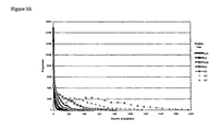
- a plot of the number of neighboring loops versus its frequency (the number of times this number of neighbors was found) using various NEIGHBOR_LIMIT is shown in Figure 10 . For most values of NEIGHBOR_LIMIT, as the number of neighboring loops increases, the frequency decreases and as the number of neighboring loops decreases, the frequency increases.
- the frequency maximum is located between 200 to 600 neighboring loops instead of locating near the lower number of neighboring loops. This means that for large NEIGHBOR_LIMIT, it is more frequent to have 200 to 600 neighbors rather than 0-100 neighbors.
- the figure also shows the maximum number of neighboring loops for a particular NEIGHBOR_LIMIT, thereby giving an indication to the similarity between the loops. For example, the maximum number of neighboring loops is 1763 with NEIGHBOR_LIMIT of 0.7, 526 with NEIGHBOR_LIMIT of 0.4 and 146 with NEIGHBOR_LIMIT of 0.25.
- the next step was to identify (given a specific loop and its neighbors) the loop that has the largest number of neighbors (a peak). That is, the loop is marked as a peak if all the neighboring loops have lower or equal number of neighboring loops.
- the number of peaks for various NEIGHBOR_LIMIT is shown in Figure 11 . The figure shows that the number of peaks varied from 7818 to 13 as the NEIGHBOR_LIMIT varied from 0.25 to 0.7. However, since peaks with the number of neighbors of less than an arbitrarily chosen low SEA_LEVEL of 20 are not interesting as they are not significantly populated, the plot also shows the number of peaks with greater than the SEA_LEVEL number of neighbors. The number of peaks with greater than the SEA_LEVEL of 20 ranges from 56 to 3, decreasing with increasing NEIGHBOR_LIMIT.
- NEIGHBOR_LIMIT To examine the implication of the choice of 0.3 for NEIGHBOR_LIMIT, we determined whether the unique peaks obtained using a higher NEIGHBOR_LIMIT are a subset of those obtained using the lower NEIGHBOR_LIMIT of 0.3. For example, if the unique peaks for the NEIGHBOUR_LlMIT of 0.4 are a subset (are similar to) the unique peaks found for the NEIGHBOR_LIMIT of 0.3 then we would expect to find structurally similar unique peaks in both datasets. To do this, we systematically pair each of the unique peaks obtained using a higher NEIGHBOR_LIMIT with the most structurally similar unique peak obtained using a NEIGHBOR_LIMIT of 0.3.
- the filtered nearest centroid sorting algorithm described in section 1.2.1.4 was utilized to refine the clustering.
- the 39 unique peaks with greater than twenty neighbors were used as initial seeds for our filtered centroid sorting algorithm using various TOLERANCE.
- the percentage of data clustered, the average intracluster-RMSD, the average intercluster RMSD and the ratio of the latter two are plotted as a function of the TOLERANCE in Figure 12 . The figure shows that as the TOLERANCE increases, the percentage of data clustered and the intra-inter-RMSD ratio increases.
- the percentage of data clustered, the average intracluster RMSD, the average intercluster RMSD and ratio of the latter two are 12%, 0.22, 0.95 and 0.11, respectively; at a TOLERANCE of 0.6 RMSD they are 71%, 0.42, 1.94 and 0.21, respectively; and at a TOLERANCE of 0.9, they are 100%, 0.51, 1.90 and 0.27, respectively. Therefore, there are opposing forces in the choice of tolerance. Higher tolerance is favored because of the greater percentage of data clustered, but is disfavored because of the higher intra to inter cluster RMSD ratio. Lower tolerance is favored because of the lower intra to inter cluster RMSD ratio but is disfavored because of the lower percentage of data clustered.
- intracluster RMSD intracluster similarity
- TOLERANCE a plot of all the loops in cluster one formulated using various tolerances are shown in Figure 13 .
- the figure shows that with an average intracluster RMSD of 0.47, which corresponds with a TOLERANCE of 0.7 and 89% of the data clustered, the members in the cluster are sufficiently similar for loop mimetic purpose.
- the numbers of loops in each of the 39 clusters obtained using a tolerance of 0.7 is plotted in Figure 14 .
- the least populated cluster has 307 loops and the most populated cluster have 1048 loops.
- An RMSD matrix is calculated to examine the performance of the clustering, by assessing the similarity within and dissimilarity between clusters (Section 1.2.2.3).
- the RMSD matrix showing the average intra- and inter-clusters RMSD for all the 39 clusters, is shown in Table 5.
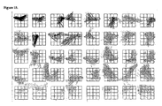
- the average intracluster RMSD of 0.47 and the vector graphs for all the clusters in Figure 15 show that the loops within a cluster have similar conformations.
- the loops between clusters are dissimilar as the average intercluster RMSD is 1.91.
- each structure is initially assigned to its own cluster of size one. Subsequently, clusters are merged if the average distance between all the structures in the two clusters fall within some threshold.
- the resulting hierarchical tree obtained by applying the average linkage-clustering algorithm on the 39 clusters, is shown in Figure 16 . All the cluster numbers used in this paper follow the order from left to right of this hierarchical tree.
- each cluster contains a unique set of loops (no loops are in more then one cluster), do the 39 clusters represent overlapping-variation from a continuous spread or do they represent distinct clusters that do not overlap in hyperspace?
- two clusters are 'distinct' if the most frequent eighty-percent of the data in one cluster does not overlap with the most frequent eighty-percent of the data in the other cluster. The overlaps were computed for each of the following thirty-two descriptors of the loop conformation.
- Each c ⁇ -c ⁇ vector pair has four distances (c ⁇ 1 -c ⁇ 2 , c ⁇ 1 -c ⁇ 2 , c ⁇ 1 -c ⁇ 2 , c ⁇ 2 -c ⁇ 2 ), so the six possible c ⁇ -c ⁇ vector pairs (1-2, 1-3, 1-4, 2-3, 2-4, 5-4, or the four c ⁇ -c ⁇ vectors in a loop results in 24 distance descriptors.
- the maximum and minimum values which delineate the most frequent eighty percent of each distribution was not computed using the mean plus and minus some standard deviation because some of the spreads were not always a 'Normal' distribution.
- the maximum and minimum was computed by first 'binning' the data with respect to each of the thirty-two descriptors mentioned earlier. Then, the bins for each descriptor were sorted based on the frequency, from most frequent to least frequent. As the program traverses down the bins, the maximum and minimum of the descriptor are stored. The traversal is stopped when the program has traversed through at least eighty percent of the data. Consequently, the stored maximum and minimum represent the values that delineate the top eighty percentage of the distribution. This method of finding maximum and minimum works well with single peak distributions. For distributions with two or more peaks, the spread covered by the maximum and minimum are over-estimated. In such case, the determination of distinct is underestimated.
- cluster X and cluster Y are considered to be overlapping.
- cluster X is considered to be distinct from cluster Y.
- This analysis shows that 737 out of a total of 741 combinations (99%) of clusters are distinct. Since the analysis was based on individual descriptors, those non-distinct clusters could be overlapping or distinct if the analysis was extended to include combinations of the descriptors.
- the protein contact surfaces are comprised of a continous sequence of amino acid residues as well as discontinuous sequences of amino acid residues.
- At least four criteria have been used in the literature to define residues that are involved in protein-protein interfaces. Two residues in two different chains are considered to be in the protein-protein interface if (1) their c ⁇ atoms are less than 9.0 ⁇ apart or (2) any atoms in one residue is within 5 ⁇ of any atom of the other residue or (3) the distance between any atom of one residue to any atom within the other residue is less than the sum of their corresponding van der Waals radii plus 0.5 ⁇ and (4) the van der Waals energy between the residues is less than -0.5 kcal/mol. The results are quite uniform between the four criteria 54 . Criterion three is used here. Furthermore, when the number of residues in an interface is less than 10, the interface is rejected because there is a high probability that this protein-protein interaction is a result of crystal packing.
- Tsai 54 have scanned 2814 PDB entries from the September 1994 release of the PDB database 31 and found 1629 two-chain interfaces. Out of the 1629 two-chain interfaces, Tsai et al 54 have extracted 351 non-redundant families through the usage of structural comparison algorithm, measure of similarity and clustering of the structures into families ( http://protein3d.ncifcrf.gov/tsai/frame/dataset.html).
- a c++ program, p-p_interface.cpp was written to extract the coordinates of the c ⁇ -c ⁇ vectors of the residues in the protein-protein interface.
- the coordinates of the c ⁇ atom was obtained by superimposing the n, c ⁇ and c' atoms of an ideal alanine onto the n, c ⁇ and c' atoms of the glycine.
- Non-Glycine residues without c ⁇ atom coordinates were not included in the dataset.
- the 350 non-redundant families gave rise to 700 protein chains that consist of up to 150 residues that form contact in a single chain. This results in a very large dataset.
- Identifying common structures in protein contact surfaces is a significant challenge.
- the first step in determining the matching frequency of a group of residues is to develop a method to compare them.
- the large size of the database excludes the root mean squared deviation (RMSD) algorithm which is computationally expensive.
- RMSD root mean squared deviation
- a simpler method commonly used in chemical and biological situations is distance geometry comparisons.
- distance geometry comparisons do not return a value of how closely related two geometries are (like an RMSD value) but instead return a match if their distances are the same within a certain tolerance.
- the geometric relationship between two residues can be represented by four "bowtie" distances ( Figure 17 ).
- the tolerance, TOL represents the maximum allowed difference accepted between these distances to record a match.
- each motif is compared against all others.
- the set of all motifs that match a particular motif, within a tolerance called family tolerance (TOL), is referred to as the family of that motif.
- TOL family tolerance
- the cardinality of that family is the matching frequency for that motif.
- the common motifs with high matching frequencies are those that make good candidates for seed points.
- 3-motifs were formed by simply considering every feasible combination of 3 residues within each chain.
- the set of feasible motifs excludes ones that contain any bowtie distance greater than 25 ⁇ , as we are only interested in common surface patches of this size.
- the data set produced for 4-motifs formed this way is too large.
- the size of the data set for 4-motifs can be greatly reduced.
- Every 4-motif is formed by 4 3-motifs.
- the group ⁇ A,B,C,D ⁇ is formed by the 4 groups ⁇ A,B,C ⁇ , ⁇ A,B,D ⁇ , ⁇ A,C,D ⁇ and ⁇ B,C,D ⁇ .
- a motif is marked as a peak if all the other motif within the family of the motif have lower or equal matching frequency.
- the algorithm for searching for peaks in the data set is given in Figure 19 . Initially the algorithm tags every motif as a peak. Subsequently, for every motif, A, in the data set, if any motif within the family of the motif A have a lower matching frequency, it is tagged as non-peak.
- the objective of clustering methods is to retrieve all related motifs about some peak motifs, with the proviso that not all motifs in the data set need be clustered.
- the simplest method for clustering motifs is a reverse scan of the data set as for the original matching algorithm. This method passes through the data set once accepting into the cluster every motif that is matched. This procedure is very similar to the PAM non-hierarchical method 55 .
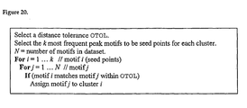
- This algorithm is called the one-pass algorithm and is outlined in Figure 20 .
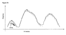
- the span of the one-pass algorithm for a landscape of motifs is illustrated in Figure 21 .
- the tolerance, OTOL assumes that the width of each hill is identical. The entire hill is rarely collected because the range of the tolerance is constant throughout the algorithm. There is a possibility that some motifs collected belong to a different hill.
- a simple method of overcoming this problem is to apply an additional tolerance to the greedy algorithm.
- the combined one-pass and greedy algorithm applies a one-pass tolerance, OTOL, to the greedy algorithm to limit its span. It applies the additional constraint that every motif in each cluster has to be within OTOL of the seed motif.
- This algorithm is outlined in Figure 24 .
- a tolerance, ' sealevel ', with respect to the matching frequency (rather than its geometry) of a motif is also effective in restricting the span of the greedy algorithm. All motifs with matching frequency below the sea level are discarded from the data set.
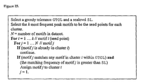
- Figure 25 shows how a sea level is applied to the single linkage algorithm. An illustration of the possible span of the algorithm is given in Figure 26 . However, selecting the correct sealevel is not always easy. If set too low it will have little effect in restricting the span of the algorithm. If set too high some peaks (and hills) will be excluded from the data set altogether. As an illustration, the first peak from the left in Figure 26 has been totally excluded from the data set and the third peak has been restricted more so than the second. Unless all peaks are about the same height the application of a sea level will handicap some hills more than others.
- each sea level for each peak can be set adaptively as shown in Figure 27 . This is a more appropriate method for restricting the span of the algorithm.
- Each sea level can be scaled according to the frequency of the peak motif.
- DSSP Domainary of Protein Secondary Structure
- This software has been utilized widely throughout the literature for the classification of protein shapes into formal secondary structure. Given the 3D coordinates of residues within a protein, DSSP classifies the shape based on its refined expert system. There are 8 different secondary structure classifications considered by DSSP. They are described in Table 14 together with the abbreviations that will be adopted in this paper. The classification 'no assignment' refers to shapes that do not fit any of the other classifications defined.
- the first step to determine the seed points for clustering was to calculate the matching frequency of each 3-motif in the dataset. This was the highest order of motif that was computationally feasible. An exhaustive combination of 3-motifs produced 9,215,424 motifs as opposed to 197,712,949 4-motifs..
- TOL Three family tolerances (TOL) of 0.25, 0.5 and 0.75 ⁇ were chosen based on a number of sample calculations. 0.25 ⁇ was the lowest tolerance that produced meaningful generalisations about structure in the dataset while 0.75 ⁇ was the highest tolerance that was computationally feasible, especially as the number of residues to be clustered increased.
- the 4-motifs were constructed. As discussed previously in the method section, these motifs were constructed based on the common 3-motifs. At this point, we eliminated the uncommon motifs by removing all motifs that have a matching frequency below the matching frequency sealevel. For example, all 3-motifs with less than 30 matching frequency were excluded before 4-motifs were created. This level was selected based on trends seen in the dataset A matching frequency sealevel of 30 is insignificant when compared against the highest matching frequency (434 for TOL 0.25 ⁇ ). We also tested a matching frequency sea levels of 20 when forming 4-motifs from the 3-motifs, and found that lowering the matching frequency sealevel had no effect on the frequency of the seed points.
- Figure 30 shows the highest matching frequency for each tolerance for each N-motif (3 ⁇ N ⁇ 7).
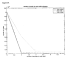
- Figure 29 shows the number of N- motifs created. The number of motifs for larger tolerances is greater because the matching frequencies are higher and hence less of the dataset is excluded.
- peak motif geometries can be extracted from the dataset ( Figure 19 ). From the dataset of peak motifs, the 30 motifs with the largest matching frequency were selected to be the seed points for the clustering stage. This value is kept constant for all motif sizes and tolerances. Although chosen arbitrarily, it almost always includes all unique motifs that have up to half the matching frequency of the highest value for that dataset. At the same time, there are not too many seed points as to get significant overlapping in the clusters. When only 30 seed points are selected, this overlapping only occurs when large tolerances are adopted for the clustering algorithms. In addition, a plot of a histogram of the dataset reveals that significant amount of the original data is covered by the 30 most common unique motifs.
- each clustering algorithm is determined by three pieces of information: the size of the clusters, the intracluster RMSD and the intercluster RMSD.
- the aim is to cluster as many motifs as possible, though the resulting clusters should contain motifs that are similar (minimise intracluster RMSD), though each cluster must differ as much as possible (increase intercluster RMSD).
- Summary table for the 4-motif, 5-motif, 6-motif and 7-motif is given in the Table 6, 8, 10 and 12, respectively.
- Information about the clustering for family tolerance 0.25 ⁇ are not presented for 6-motifs or larger because the dataset was too small to extract meaningful clusters.
- the summary tables give the sum of the size of the clusters and the sum of the number of unique motifs within those clusters.
- the difference between the sum of the size of the clusters and the sum of the unique motifs in clusters give the number of motifs that occur in more than one cluster.
- the intracluster and intercluster RMSD are the average for each algorithm.
- Table 7, 9, 11 and 13 contain the intracluster RMSD, the average RMSD of each motif in the cluster superimposed onto the average motif for that cluster (along the main diagonal), and the intercluster RMSD, the average RMSD of all motifs against the mean motif of other cluster (entries off the main diagonal).
- the size of each cluster is presented.
- the representative clusters for each N-motif is selected based on a simple criteria: select the clustering technique producing the largest amount of data, while having small intracluster RMSD and large intercluster RMSD.
- a small intracluster RMSD is less than 0.5 ⁇ and a large intercluster RMSD is greater than 2.0 ⁇ .
- the summary of results for 5- motifs is given in Table 8.
- the selected representative clusters in this case were the greedy algorithm, family tolerance 0.75, greedy tolerance 0.7 ⁇ and sealevel 0.125 of the seed matching frequency.
- An example of a cluster of 5-residue motifs ( C30 ) is given in Figure 32 .
- Average clustering results for 6- motifs are presented in Table 10.
- the selected method in this case was the greedy algorithm, family tolerance 0.75 ⁇ , greedy tolerance 0.7 ⁇ and sealevel 0.125 times the peak matching frequency.
- Specific cluster information about the methods are presented in Table 11.
- a representative cluster for the selected clustering algorithm C1 is given in Figure 33 .
- the seeds or clusters do not necessarily belong to a single ⁇ -helix because the residues flanking between the residues in the motif may not be ⁇ -helical. Due to possible uncertainty with the DSSP classification, an ⁇ -helix is considered broken when flanked by two or more consecutive non ⁇ -helical residues.
- Table 19 records the proportion of motifs in each cluster that are not single ⁇ -helix. Except for cluster C2 of the 4- motifs (of which 99% are non-helical), almost all other motifs are single ⁇ -helix.
- Table 21 contains a summary of the clusters retrieved using a variety of methods with the new seeds.
- the most successful clustering methods of the previous analysis were adopted as starting points for this analysis. These results show that there is a strong trend towards clusters becoming more distinct as the size of the motif increases.
- 4-residue motifs there is significant sharing of motifs between clusters with many having quite a large intracluster RMSD.
- the greedy tolerance could be extended to 1.1 ⁇ for 6-residue motifs with the intracluster RMSD remaining very low. This is in contrast to the highest tolerance of 0.7 ⁇ that could be adopted for the original set of seeds.
- Table 23 presents the distribution of different types of secondary structures for the new 4-residue motif clusters. Even though the seeds of each of these clusters are classified as 'not a single ⁇ -helix', a large proportion of motifs within three clusters are ⁇ -helix. Table 24 presents the proportion of motifs in each of the new clusters that are not a single ⁇ -helix. Less than 20% of motifs of cluster C5, C17 and C25 are not a single ⁇ -helix and more than 90% of residues of these clusters are classified as ⁇ -helix.
- Clusters that have a high proportion of motifs with no assignment to formal secondary structure, such as C2 , C3 , C4 , C7 , C10, C12 and C16 have relatively small size (the largest has just 26 members) and relatively low intracluster RMSD. Within this group, the average intracluster RMSD is 0.28 ⁇ as opposed to the average intracluster RMSD of 0.52 ⁇ for the entire set.
- Table 25 presents the distribution of secondary structure classifications for 7-residue motifs. Only clusters C1, C 2 and C 3 have motifs whose component residues are not entirely classified 'no assignment'. These three clusters have average intracluster RMSD of 0.41 ⁇ which is much larger than the average intracluster RMSD for the entire set of 0.26 ⁇ . This correlation suggests these clusters that contain motifs with no formal secondary structure assignment, have shape that is highly unique to any other motifs in the dataset.
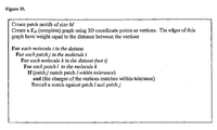
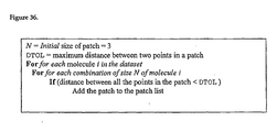
- the basic algorithm for the clustering of surface patches is similar to that for clustering discontinuous protein surfaces. Firstly, snapshots of the protein surface, called patch motifs, is generated. A patch motif containing N grid points is referred to as an N- patch. The smallest patch size that will be considered in this study is the 3-patch. The algorithm for the construction of 3-patches is given in Figure 36 .
- Figure 35 describe the algorithm for determining the matching frequency of each patch motif. Again, an RMSD superimposition of these motifs is too computationally expensive because of the size and the number of patches.
- a distance matrix is constructed so that the shape of the patches can be easily compared. This distance matrix is calculated for an N- patch by creating a complete graph K N whose vertices are the grid points and edges are weighted by the Euclidian distance between each pair of vertices.
- An illustration of a complete graph K 9 constructed for a 9-patch is given in Figure 38 .
- a number of quick and simple comparisons can be made between pairs of patches before an exhaustive check should take place. This is to improve the computational feasibility of the problem. The first is to compare the charges of each grid point before comparing distances. If the charges don't match within the charge tolerance, there is no need to check if the edge distances match. This is a much easier calculation. Another is to check if the longest and shortest edge distances of the pair of patches match. If they don't then the geometric structure of the patches is different. Finally, there may be some distances of the distance matrix that remain constant for all patches because of the way the grid was originally constructed. This may remove the need to consider certain orientations of patches when being compared.
- N+1-patches will be constructed based on N-patches in similar manner to the higher order motif build-up procedure for the discontinuous surfaces described earlier. Patches that are less than a defined matching frequency sealevel will be removed from the dataset. This reduces the number of redundant higher order patches that will be created.
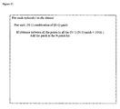
- the algorithm for the creation of higher order patches is given in Figure 37 . In this algorithm, each new N -patch is created from (N-1) ( N -1)-patches.
- seeds and clusters can be obtained as described in the previous sections.
- the present inventors have clustered the side chain positions of ⁇ -turns, loops and protein contact surfaces. This has resulted in the identification of 9, 39 and 240 highly populated motifs for ⁇ -turns, loops and protein contact surfaces, respectively. As an example, the coordinate of the 5 th least popular cluster of all these motifs are given in Table 26. These motifs define common spatial elements of protein surfaces. Our objective is to use these motifs to design libraries of molecules. Consequently, these motifs are used as biological descriptors in library design, and the resulting libraries will mimic common protein shapes. In high throughput screening, such libraries will be a valuable resource for the development of new lead compounds.
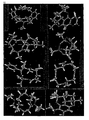
- Figure 39a shows some of the scaffolds that match the ⁇ -turn conformations
- Figure 39b shows some of the scaffolds that match the common loop conformations
- Figure 39c shows a scaffold that match a common six-residues protein-protein interaction surface.
Landscapes
- Life Sciences & Earth Sciences (AREA)
- Engineering & Computer Science (AREA)
- Health & Medical Sciences (AREA)
- Physics & Mathematics (AREA)
- Chemical & Material Sciences (AREA)
- Bioinformatics & Computational Biology (AREA)
- Theoretical Computer Science (AREA)
- Spectroscopy & Molecular Physics (AREA)
- General Health & Medical Sciences (AREA)
- Bioinformatics & Cheminformatics (AREA)
- Evolutionary Biology (AREA)
- Biophysics (AREA)
- Biotechnology (AREA)
- Library & Information Science (AREA)
- Medical Informatics (AREA)
- Crystallography & Structural Chemistry (AREA)
- Biochemistry (AREA)
- Molecular Biology (AREA)
- Medicinal Chemistry (AREA)
- Computing Systems (AREA)
- Peptides Or Proteins (AREA)
- Information Retrieval, Db Structures And Fs Structures Therefor (AREA)
- Materials For Medical Uses (AREA)
- Investigating Or Analysing Biological Materials (AREA)
Claims (29)
- Computerimplementiertes Verfahren zum Erzeugen einer Beschreibung einer gemeinsamen dreidimensionalen Proteinoberflächenform, das die folgenden Schritte umfasst:(i) Identifizieren einer dreidimensionalen Oberflächenform jedes von mehreren Proteinen, wobei jede dreidimensionale Oberflächenform durch einen Ort und eine Orientierung einer Seitenkette von zwei oder mehr Aminosäuren jedes der mehreren Proteine repräsentiert wird; und(ii) Erzeugen eines oder mehrerer Deskriptoren, wobei jeder Deskriptor eine gemeinsame Oberflächenform repräsentiert, die aus Entsprechenden der dreidimensionalen Oberflächenformen von drei oder mehr Proteinen der mehreren Proteine abgeleitet wird.
- Verfahren nach Anspruch 1, wobei drei oder mehr Proteine nicht homologe Proteine mit einer Homologie von nicht mehr als 25 % sind.
- Verfahren nach Anspruch 1, wobei der oder jeder Deskriptor einen gemeinsamen Ort und eine gemeinsame Orientierung entsprechender Seitenketten der drei oder mehr Aminosäuren jedes der drei oder mehr Proteine repräsentiert.
- Verfahren nach Anspruch 3, wobei der Ort und die Orientierung jeder Aminosäuren-Seitenkette im dreidimensionalen Raum (3D-Raum) vorhanden sind.
- Verfahren nach Anspruch 4, wobei jede Aminosäuren-Seitenkette, die verwendet wird, um den Deskriptor zu erzeugen, als ein Cα-Cβ-Vektor vereinfacht wird.
- Verfahren nach Anspruch 1, wobei jede dreidimensionale Oberflächenform, die im Schritt (i) identifiziert wird, als ein geladener Oberflächenbereich jedes Proteins repräsentiert wird.
- Verfahren nach Anspruch 6, wobei im Schritt (ii) jeder Deskriptor einen gemeinsamen geladenen Oberflächenbereich jedes Proteins repräsentiert.
- Verfahren nach Anspruch 7, wobei jeder geladene Oberflächenbereich durch wenigstens vier Gitterpunkte repräsentiert wird.
- Verfahren nach Anspruch 8, wobei entsprechende Gitterpunkte im dreidimensionalen Raum (3D-Raum) um 0,2 bis 2,0 Ångström beabstandet sind.
- Verfahren nach Anspruch 9, wobei entsprechende Gitterpunkte im dreidimensionalen Raum (3D-Raum) um 0,5 bis 1,5 Ångström beabstandet sind.
- Verfahren nach Anspruch 1, wobei die dreidimensionale Oberflächenform wenigstens ein Teil eines Strukturmerkmals jedes der Proteine ist.
- Verfahren nach Anspruch 11, wobei das Strukturmerkmal eine β-Windung, eine Schleife oder eine Kontaktoberfläche ist oder enthält.
- Verfahren nach Anspruch 11, wobei das Strukturmerkmal eine Schleife oder eine Kontaktoberfläche ist oder enthält.
- Verfahren nach Anspruch 12, wobei die Kontaktoberfläche eine oder mehrere diskontinuierliche und/oder kontinuierliche Oberflächen enthält.
- Verfahren nach Anspruch 12, wobei der Deskriptor den Ort und die Orientierung einer Seitenkette von vier β-Windungs- oder Schleifen-Aminosäuren repräsentiert.
- Verfahren nach Anspruch 12, wobei der Deskriptor den Ort und die Orientierung einer Seitenkette von wenigstens drei Aminosäuren einer Kontaktoberfläche repräsentiert.
- Verfahren nach Anspruch 16, wobei der Deskriptor den Ort und die Orientierung einer Seitenkette von vier, fünf, sechs oder sieben Aminosäuren-Seitenketten einer Kontaktoberfläche repräsentiert.
- Computerimplementiertes Verfahren zum Identifizieren eines oder mehrerer Moleküle mit einer gemeinsamen dreidimensionalen Proteinoberflächenform, wobei das Verfahren die folgenden Schritte umfasst:(i) Erzeugen eines oder mehrerer Deskriptoren gemäß dem Verfahren nach Anspruch 1;(ii) Erzeugen einer Abfrage unter Verwendung des einen oder der mehreren Deskriptoren, die im Schritt (i) erzeugt werden; und(iii) Verwenden der Abfrage, um eine Datenbank zu durchsuchen und um dadurch einen oder mehrere Einträge in der Datenbank zu identifizieren, die einem oder mehreren Molekülen entsprechen, die jeweils zu dem Deskriptor passen.
- Verfahren nach Anspruch 18, wobei im Schritt (ii) der Deskriptor einen gemeinsamen Ort und eine gemeinsame Orientierung einer Aminosäuren-Seitenkette von zwei der mehr Aminosäuren jedes von drei oder mehr Proteinen repräsentiert.
- Verfahren nach Anspruch 18, wobei im Schritt (ii) der Deskriptor eine gemeinsame Proteinoberflächenladungsform der drei oder mehr Proteine repräsentiert.
- Verfahren nach Anspruch 18, wobei im Schritt (ii) die Abfrage umfasst:(a) einen Deskriptor, der einen gemeinsamen Ort und eine gemeinsame Orientierung einer Seitenkette von zwei oder mehr Aminosäuren jedes der drei oder mehr Proteine repräsentiert; und(b) einen Deskriptor, der eine gemeinsame Proteinoberflächenladungsform der drei oder mehr Proteine repräsentiert.
- Verfahren nach Anspruch 18, wobei jede Aminosäuren-Seitenkette, die verwendet wird, um den Deskriptor zu erzeugen, als einen Cα-Cβ-Vektor vereinfacht ist.
- Verfahren nach Anspruch 22, wobei die Cα-Cβ-Vektoren der Abfrage als eine Abstandsmatrix repräsentiert sind.
- Computerimplementiertes Verfahren zum Erzeugen einer Bibliothek von Molekülen, das die folgenden Schritte umfasst:(i) Erzeugen eines oder mehrerer Deskriptoren gemäß dem Verfahren nach Anspruch 1;(ii) Durchsuchen einer Datenbank, um einen oder mehrere Einträge zu identifizieren, die einem oder mehreren Molekülen entsprechen, die jeweils zu dem einen oder den mehreren Deskriptoren passen, die im Schritt (i) erzeugt werden; und(iii) Verwenden wenigstens eines des einen oder der mehreren Moleküle, die im Schritt (ii) identifiziert werden, um eine Bibliothek von Molekülen zu erzeugen.
- Verfahren nach Anspruch 24, wobei die Bibliothek von Molekülen eine virtuelle Bibliothek ist.
- Verfahren nach Anspruch 24, wobei die Bibliothek von Molekülen eine synthetische chemische Bibliothek ist.
- Verfahren zum Entwickeln eines oder mehrerer Moleküle, das die folgenden Schritte umfasst:(i) Erzeugen eines oder mehrerer Deskriptoren gemäß dem Verfahren nach Anspruch 1; und(ii) Entwickeln eines oder mehrerer Moleküle, die jeweils eines oder mehrere Strukturmerkmale des oder jedes Deskriptors in (i) aufweisen.
- Verfahren nach Anspruch 27, wobei der oder jeder Deskriptor einen gemeinsamen Ort und eine gemeinsame Orientierung einer Seitenkette von zwei oder mehr Aminosäuren jedes der drei oder mehr Proteine repräsentiert.
- Verfahren nach Anspruch 27, wobei der oder jeder Deskriptor eine gemeinsame Proteinoberflächenladungsform der drei oder mehr Proteine repräsentiert.
Applications Claiming Priority (3)
| Application Number | Priority Date | Filing Date | Title |
|---|---|---|---|
| AUPS0397A AUPS039702A0 (en) | 2002-02-08 | 2002-02-08 | Common protein surface shapes and uses therefor |
| AUPS039702 | 2002-02-08 | ||
| PCT/AU2003/000137 WO2003066678A1 (en) | 2002-02-08 | 2003-02-10 | Common protein surface shapes and uses therefor |
Publications (3)
| Publication Number | Publication Date |
|---|---|
| EP1483291A1 EP1483291A1 (de) | 2004-12-08 |
| EP1483291A4 EP1483291A4 (de) | 2007-03-14 |
| EP1483291B1 true EP1483291B1 (de) | 2011-07-06 |
Family
ID=3833998
Family Applications (1)
| Application Number | Title | Priority Date | Filing Date |
|---|---|---|---|
| EP03700720A Expired - Lifetime EP1483291B1 (de) | 2002-02-08 | 2003-02-10 | Herkömmliche formen von proteinoberflächen und deren verwendungen |
Country Status (7)
| Country | Link |
|---|---|
| US (2) | US20050154533A1 (de) |
| EP (1) | EP1483291B1 (de) |
| JP (1) | JP2005529382A (de) |
| AT (1) | ATE515748T1 (de) |
| AU (1) | AUPS039702A0 (de) |
| CA (1) | CA2476274C (de) |
| WO (1) | WO2003066678A1 (de) |
Families Citing this family (22)
| Publication number | Priority date | Publication date | Assignee | Title |
|---|---|---|---|---|
| JP2005250721A (ja) * | 2004-03-03 | 2005-09-15 | Hitachi High-Technologies Corp | 蛋白質または高分子複合体の検索・照合方法及び装置 |
| US9165052B2 (en) * | 2009-11-24 | 2015-10-20 | Zymeworks Inc. | Density based clustering for multidimensional data |
| US9273093B2 (en) | 2012-10-11 | 2016-03-01 | Protagonist Therapeutics, Inc. | α4β7 peptide dimer antagonists |
| US9244946B2 (en) | 2012-11-26 | 2016-01-26 | International Business Machines Corporation | Data mining shape based data |
| EP4091624A1 (de) | 2013-03-15 | 2022-11-23 | Protagonist Therapeutics, Inc. | Hepcidin-analoga und verwendungen davon |
| HRP20211448T1 (hr) | 2014-05-16 | 2021-12-24 | Protagonist Therapeutics, Inc. | Alfa4beta7 integrin tioeter peptidni antagonisti |
| CN107206254B (zh) | 2014-07-17 | 2021-08-24 | 领导医疗有限公司 | 白细胞介素-23受体的口服肽抑制剂以及其治疗炎症性肠病的用途 |
| US10301371B2 (en) | 2014-10-01 | 2019-05-28 | Protagonist Therapeutics, Inc. | Cyclic monomer and dimer peptides having integrin antagonist activity |
| WO2016054411A1 (en) | 2014-10-01 | 2016-04-07 | Protagonist Therapeutics, Inc. | NOVEL α4β7 PEPTIDE MONOMER AND DIMER ANTAGONISTS |
| US10787490B2 (en) | 2015-07-15 | 2020-09-29 | Protaganist Therapeutics, Inc. | Peptide inhibitors of interleukin-23 receptor and their use to treat inflammatory diseases |
| US20190002503A1 (en) | 2015-12-30 | 2019-01-03 | Protagonist Therapeutics, Inc. | Analogues of hepcidin mimetics with improved in vivo half lives |
| CA3017926C (en) | 2016-03-23 | 2023-10-10 | Protagonist Therapeutics, Inc. | Methods for synthesizing .alpha.4.beta.7 peptide antagonists |
| EP3681900A4 (de) | 2017-09-11 | 2021-09-08 | Protagonist Therapeutics, Inc. | Opioidagonistpeptide und verwendungen davon |
| CA3089868A1 (en) | 2018-02-08 | 2019-08-15 | Protagonist Therapeutics, Inc. | Conjugated hepcidin mimetics |
| JP7102790B2 (ja) | 2018-03-07 | 2022-07-20 | 富士通株式会社 | データ生成方法、データ生成プログラム及び情報処理装置 |
| WO2020014646A1 (en) | 2018-07-12 | 2020-01-16 | Protagonist Therapeutics, Inc. | Peptide inhibitors of interleukin-23 receptor and their use to treat inflammatory diseases |
| JP7534382B2 (ja) | 2019-07-10 | 2024-08-14 | プロタゴニスト セラピューティクス, インコーポレイテッド | インターロイキン-23受容体のペプチド阻害剤及び炎症性疾患を治療するためのその使用 |
| AU2021209086A1 (en) | 2020-01-15 | 2022-08-04 | Janssen Biotech, Inc. | Peptide inhibitors of interleukin-23 receptor and their use to treat inflammatory diseases |
| CA3167751A1 (en) | 2020-01-15 | 2021-07-22 | Janssen Biotech, Inc. | Peptide inhibitors of interleukin-23 receptor and their use to treat inflammatory diseases |
| JP7397239B2 (ja) | 2020-11-20 | 2023-12-12 | ヤンセン ファーマシューティカ エヌ.ベー. | インターロイキン-23受容体のペプチド阻害剤の組成物 |
| EP4370146A4 (de) | 2021-07-14 | 2025-05-21 | Janssen Biotech, Inc. | Lipidierte peptidinhibitoren des interleukin-23-rezeptors |
| JPWO2024224580A1 (de) * | 2023-04-27 | 2024-10-31 |
Family Cites Families (5)
| Publication number | Priority date | Publication date | Assignee | Title |
|---|---|---|---|---|
| US5223409A (en) * | 1988-09-02 | 1993-06-29 | Protein Engineering Corp. | Directed evolution of novel binding proteins |
| NZ510230A (en) * | 1998-08-25 | 2004-01-30 | Scripps Research Inst | Predicting protein function by electronic comparison of functional site descriptors |
| AUPP660698A0 (en) * | 1998-10-21 | 1998-11-12 | University Of Queensland, The | A method of protein engineering |
| WO2001037147A2 (en) * | 1999-11-03 | 2001-05-25 | Algonomics Nv | Apparatus and method for structure-based prediction of amino acid sequences |
| AU2001268506A1 (en) * | 2000-06-16 | 2002-01-02 | Neogenesis Pharmaceuticals Inc. | System and method for evaluating pockets in protein |
-
2002
- 2002-02-08 AU AUPS0397A patent/AUPS039702A0/en not_active Abandoned
-
2003
- 2003-02-10 AT AT03700720T patent/ATE515748T1/de not_active IP Right Cessation
- 2003-02-10 WO PCT/AU2003/000137 patent/WO2003066678A1/en not_active Ceased
- 2003-02-10 CA CA2476274A patent/CA2476274C/en not_active Expired - Fee Related
- 2003-02-10 US US10/503,655 patent/US20050154533A1/en not_active Abandoned
- 2003-02-10 EP EP03700720A patent/EP1483291B1/de not_active Expired - Lifetime
- 2003-02-10 JP JP2003566049A patent/JP2005529382A/ja active Pending
-
2009
- 2009-08-17 US US12/542,427 patent/US8635027B2/en not_active Expired - Fee Related
Also Published As
| Publication number | Publication date |
|---|---|
| US20050154533A1 (en) | 2005-07-14 |
| US8635027B2 (en) | 2014-01-21 |
| US20090318311A1 (en) | 2009-12-24 |
| AUPS039702A0 (en) | 2002-03-07 |
| CA2476274A1 (en) | 2003-08-14 |
| EP1483291A1 (de) | 2004-12-08 |
| JP2005529382A (ja) | 2005-09-29 |
| CA2476274C (en) | 2013-07-30 |
| EP1483291A4 (de) | 2007-03-14 |
| WO2003066678A1 (en) | 2003-08-14 |
| ATE515748T1 (de) | 2011-07-15 |
Similar Documents
| Publication | Publication Date | Title |
|---|---|---|
| US8635027B2 (en) | Common protein surface shapes and uses therefor | |
| Fu et al. | Modeling backbone flexibility to achieve sequence diversity: the design of novel α-helical ligands for Bcl-xL | |
| Etchebest et al. | A structural alphabet for local protein structures: improved prediction methods | |
| Wintjens et al. | Automatic classification and analysis of αα-turn motifs in proteins | |
| Lamb et al. | Design, docking, and evaluation of multiple libraries against multiple targets | |
| Weber | Evolutionary combinatorial chemistry: application of genetic algorithms | |
| Kiemer et al. | WI‐PHI: a weighted yeast interactome enriched for direct physical interactions | |
| Halperin et al. | SiteLight: binding‐site prediction using phage display libraries | |
| CN101855392A (zh) | 虚拟筛选装置及虚拟筛选方法 | |
| Deane et al. | A novel exhaustive search algorithm for predicting the conformation of polypeptide segments in proteins | |
| Du et al. | Have we seen all structures corresponding to short protein fragments in the Protein Data Bank? An update | |
| US20070134662A1 (en) | Structural interaction fingerprint | |
| Hunter et al. | Protein fragment clustering and canonical local shapes | |
| Mönnigmann et al. | Protein loop structure prediction with flexible stem geometries | |
| Eyal et al. | Protein side‐chain rearrangement in regions of point mutations | |
| US20070184487A1 (en) | Compositions and methods for design of non-immunogenic proteins | |
| Lessel et al. | Importance of anchor group positioning in protein loop prediction | |
| Brown et al. | Genetic diversity: applications of evolutionary algorithms to combinatorial library design | |
| Fraga et al. | An amino acid code to define a protein's tertiary packing surface | |
| CA2440443A1 (en) | Computer-based strategy for peptide and protein conformational ensemble enumeration and ligand affinity analysis | |
| EP1471443B1 (de) | Verfahren zum konstruieren der stereostruktur eines proteins mit mehreren ketten | |
| Hadarovich et al. | Structural motifs in protein cores and at protein–protein interfaces are different | |
| Artymiuk et al. | Searching techniques for databases of protein secondary structures | |
| Tran et al. | Topological side-chain classification of β-turns: Ideal motifs for peptidomimetic development | |
| CA2537872A1 (en) | Methods for establishing and analyzing the conformation of amino acid sequences |
Legal Events
| Date | Code | Title | Description |
|---|---|---|---|
| PUAI | Public reference made under article 153(3) epc to a published international application that has entered the european phase |
Free format text: ORIGINAL CODE: 0009012 |
|
| 17P | Request for examination filed |
Effective date: 20040908 |
|
| AK | Designated contracting states |
Kind code of ref document: A1 Designated state(s): AT BE BG CH CY CZ DE DK EE ES FI FR GB GR HU IE IT LI LU MC NL PT SE SI SK TR |
|
| AX | Request for extension of the european patent |
Extension state: AL LT LV MK RO |
|
| RIC1 | Information provided on ipc code assigned before grant |
Ipc: G06F 19/00 20060101AFI20070131BHEP |
|
| A4 | Supplementary search report drawn up and despatched |
Effective date: 20070208 |
|
| 17Q | First examination report despatched |
Effective date: 20090116 |
|
| GRAP | Despatch of communication of intention to grant a patent |
Free format text: ORIGINAL CODE: EPIDOSNIGR1 |
|
| GRAS | Grant fee paid |
Free format text: ORIGINAL CODE: EPIDOSNIGR3 |
|
| GRAA | (expected) grant |
Free format text: ORIGINAL CODE: 0009210 |
|
| AK | Designated contracting states |
Kind code of ref document: B1 Designated state(s): AT BE BG CH CY CZ DE DK EE ES FI FR GB GR HU IE IT LI LU MC NL PT SE SI SK TR |
|
| REG | Reference to a national code |
Ref country code: GB Ref legal event code: FG4D |
|
| REG | Reference to a national code |
Ref country code: CH Ref legal event code: EP |
|
| REG | Reference to a national code |
Ref country code: IE Ref legal event code: FG4D |
|
| REG | Reference to a national code |
Ref country code: DE Ref legal event code: R096 Ref document number: 60337620 Country of ref document: DE Effective date: 20110908 |
|
| REG | Reference to a national code |
Ref country code: NL Ref legal event code: VDEP Effective date: 20110706 |
|
| PG25 | Lapsed in a contracting state [announced via postgrant information from national office to epo] |
Ref country code: SI Free format text: LAPSE BECAUSE OF FAILURE TO SUBMIT A TRANSLATION OF THE DESCRIPTION OR TO PAY THE FEE WITHIN THE PRESCRIBED TIME-LIMIT Effective date: 20110706 |
|
| REG | Reference to a national code |
Ref country code: AT Ref legal event code: MK05 Ref document number: 515748 Country of ref document: AT Kind code of ref document: T Effective date: 20110706 |
|
| PG25 | Lapsed in a contracting state [announced via postgrant information from national office to epo] |
Ref country code: SE Free format text: LAPSE BECAUSE OF FAILURE TO SUBMIT A TRANSLATION OF THE DESCRIPTION OR TO PAY THE FEE WITHIN THE PRESCRIBED TIME-LIMIT Effective date: 20110706 Ref country code: BE Free format text: LAPSE BECAUSE OF FAILURE TO SUBMIT A TRANSLATION OF THE DESCRIPTION OR TO PAY THE FEE WITHIN THE PRESCRIBED TIME-LIMIT Effective date: 20110706 Ref country code: FI Free format text: LAPSE BECAUSE OF FAILURE TO SUBMIT A TRANSLATION OF THE DESCRIPTION OR TO PAY THE FEE WITHIN THE PRESCRIBED TIME-LIMIT Effective date: 20110706 Ref country code: PT Free format text: LAPSE BECAUSE OF FAILURE TO SUBMIT A TRANSLATION OF THE DESCRIPTION OR TO PAY THE FEE WITHIN THE PRESCRIBED TIME-LIMIT Effective date: 20111107 Ref country code: NL Free format text: LAPSE BECAUSE OF FAILURE TO SUBMIT A TRANSLATION OF THE DESCRIPTION OR TO PAY THE FEE WITHIN THE PRESCRIBED TIME-LIMIT Effective date: 20110706 |
|
| PG25 | Lapsed in a contracting state [announced via postgrant information from national office to epo] |
Ref country code: CY Free format text: LAPSE BECAUSE OF FAILURE TO SUBMIT A TRANSLATION OF THE DESCRIPTION OR TO PAY THE FEE WITHIN THE PRESCRIBED TIME-LIMIT Effective date: 20110706 Ref country code: AT Free format text: LAPSE BECAUSE OF FAILURE TO SUBMIT A TRANSLATION OF THE DESCRIPTION OR TO PAY THE FEE WITHIN THE PRESCRIBED TIME-LIMIT Effective date: 20110706 Ref country code: GR Free format text: LAPSE BECAUSE OF FAILURE TO SUBMIT A TRANSLATION OF THE DESCRIPTION OR TO PAY THE FEE WITHIN THE PRESCRIBED TIME-LIMIT Effective date: 20111007 |
|
| PG25 | Lapsed in a contracting state [announced via postgrant information from national office to epo] |
Ref country code: CZ Free format text: LAPSE BECAUSE OF FAILURE TO SUBMIT A TRANSLATION OF THE DESCRIPTION OR TO PAY THE FEE WITHIN THE PRESCRIBED TIME-LIMIT Effective date: 20110706 Ref country code: SK Free format text: LAPSE BECAUSE OF FAILURE TO SUBMIT A TRANSLATION OF THE DESCRIPTION OR TO PAY THE FEE WITHIN THE PRESCRIBED TIME-LIMIT Effective date: 20110706 |
|
| PLBE | No opposition filed within time limit |
Free format text: ORIGINAL CODE: 0009261 |
|
| STAA | Information on the status of an ep patent application or granted ep patent |
Free format text: STATUS: NO OPPOSITION FILED WITHIN TIME LIMIT |
|
| PG25 | Lapsed in a contracting state [announced via postgrant information from national office to epo] |
Ref country code: EE Free format text: LAPSE BECAUSE OF FAILURE TO SUBMIT A TRANSLATION OF THE DESCRIPTION OR TO PAY THE FEE WITHIN THE PRESCRIBED TIME-LIMIT Effective date: 20110706 Ref country code: IT Free format text: LAPSE BECAUSE OF FAILURE TO SUBMIT A TRANSLATION OF THE DESCRIPTION OR TO PAY THE FEE WITHIN THE PRESCRIBED TIME-LIMIT Effective date: 20110706 |
|
| 26N | No opposition filed |
Effective date: 20120411 |
|
| PG25 | Lapsed in a contracting state [announced via postgrant information from national office to epo] |
Ref country code: DK Free format text: LAPSE BECAUSE OF FAILURE TO SUBMIT A TRANSLATION OF THE DESCRIPTION OR TO PAY THE FEE WITHIN THE PRESCRIBED TIME-LIMIT Effective date: 20110706 |
|
| REG | Reference to a national code |
Ref country code: DE Ref legal event code: R097 Ref document number: 60337620 Country of ref document: DE Effective date: 20120411 |
|
| PG25 | Lapsed in a contracting state [announced via postgrant information from national office to epo] |
Ref country code: MC Free format text: LAPSE BECAUSE OF NON-PAYMENT OF DUE FEES Effective date: 20120229 |
|
| REG | Reference to a national code |
Ref country code: CH Ref legal event code: PL |
|
| PG25 | Lapsed in a contracting state [announced via postgrant information from national office to epo] |
Ref country code: CH Free format text: LAPSE BECAUSE OF NON-PAYMENT OF DUE FEES Effective date: 20120229 Ref country code: LI Free format text: LAPSE BECAUSE OF NON-PAYMENT OF DUE FEES Effective date: 20120229 |
|
| REG | Reference to a national code |
Ref country code: IE Ref legal event code: MM4A |
|
| PG25 | Lapsed in a contracting state [announced via postgrant information from national office to epo] |
Ref country code: IE Free format text: LAPSE BECAUSE OF NON-PAYMENT OF DUE FEES Effective date: 20120210 |
|
| PG25 | Lapsed in a contracting state [announced via postgrant information from national office to epo] |
Ref country code: ES Free format text: LAPSE BECAUSE OF FAILURE TO SUBMIT A TRANSLATION OF THE DESCRIPTION OR TO PAY THE FEE WITHIN THE PRESCRIBED TIME-LIMIT Effective date: 20111017 |
|
| PG25 | Lapsed in a contracting state [announced via postgrant information from national office to epo] |
Ref country code: BG Free format text: LAPSE BECAUSE OF FAILURE TO SUBMIT A TRANSLATION OF THE DESCRIPTION OR TO PAY THE FEE WITHIN THE PRESCRIBED TIME-LIMIT Effective date: 20111006 |
|
| PG25 | Lapsed in a contracting state [announced via postgrant information from national office to epo] |
Ref country code: TR Free format text: LAPSE BECAUSE OF FAILURE TO SUBMIT A TRANSLATION OF THE DESCRIPTION OR TO PAY THE FEE WITHIN THE PRESCRIBED TIME-LIMIT Effective date: 20110706 |
|
| PG25 | Lapsed in a contracting state [announced via postgrant information from national office to epo] |
Ref country code: LU Free format text: LAPSE BECAUSE OF NON-PAYMENT OF DUE FEES Effective date: 20120210 |
|
| PG25 | Lapsed in a contracting state [announced via postgrant information from national office to epo] |
Ref country code: HU Free format text: LAPSE BECAUSE OF FAILURE TO SUBMIT A TRANSLATION OF THE DESCRIPTION OR TO PAY THE FEE WITHIN THE PRESCRIBED TIME-LIMIT Effective date: 20030210 |
|
| REG | Reference to a national code |
Ref country code: FR Ref legal event code: PLFP Year of fee payment: 13 |
|
| REG | Reference to a national code |
Ref country code: FR Ref legal event code: PLFP Year of fee payment: 14 |
|
| REG | Reference to a national code |
Ref country code: FR Ref legal event code: PLFP Year of fee payment: 15 |
|
| REG | Reference to a national code |
Ref country code: FR Ref legal event code: PLFP Year of fee payment: 16 |
|
| REG | Reference to a national code |
Ref country code: DE Ref legal event code: R079 Ref document number: 60337620 Country of ref document: DE Free format text: PREVIOUS MAIN CLASS: G06F0019000000 Ipc: G16Z0099000000 |
|
| PGFP | Annual fee paid to national office [announced via postgrant information from national office to epo] |
Ref country code: DE Payment date: 20190226 Year of fee payment: 17 Ref country code: GB Payment date: 20190208 Year of fee payment: 17 |
|
| PGFP | Annual fee paid to national office [announced via postgrant information from national office to epo] |
Ref country code: FR Payment date: 20190225 Year of fee payment: 17 |
|
| REG | Reference to a national code |
Ref country code: DE Ref legal event code: R119 Ref document number: 60337620 Country of ref document: DE |
|
| GBPC | Gb: european patent ceased through non-payment of renewal fee |
Effective date: 20200210 |
|
| PG25 | Lapsed in a contracting state [announced via postgrant information from national office to epo] |
Ref country code: GB Free format text: LAPSE BECAUSE OF NON-PAYMENT OF DUE FEES Effective date: 20200210 Ref country code: FR Free format text: LAPSE BECAUSE OF NON-PAYMENT OF DUE FEES Effective date: 20200229 Ref country code: DE Free format text: LAPSE BECAUSE OF NON-PAYMENT OF DUE FEES Effective date: 20200901 |