EP1364154B1 - Verfahren zur erkennung und ortung von leckagen in rohrleitungen - Google Patents
Verfahren zur erkennung und ortung von leckagen in rohrleitungen Download PDFInfo
- Publication number
- EP1364154B1 EP1364154B1 EP02701435A EP02701435A EP1364154B1 EP 1364154 B1 EP1364154 B1 EP 1364154B1 EP 02701435 A EP02701435 A EP 02701435A EP 02701435 A EP02701435 A EP 02701435A EP 1364154 B1 EP1364154 B1 EP 1364154B1
- Authority
- EP
- European Patent Office
- Prior art keywords
- network
- burst
- leakage
- icf
- node
- Prior art date
- Legal status (The legal status is an assumption and is not a legal conclusion. Google has not performed a legal analysis and makes no representation as to the accuracy of the status listed.)
- Expired - Lifetime
Links
- 238000000034 method Methods 0.000 claims abstract description 98
- 238000003012 network analysis Methods 0.000 claims abstract description 27
- 238000009826 distribution Methods 0.000 claims description 45
- 230000008569 process Effects 0.000 claims description 12
- 230000006872 improvement Effects 0.000 claims description 7
- 239000000463 material Substances 0.000 claims description 6
- 239000003607 modifier Substances 0.000 claims description 2
- 238000012935 Averaging Methods 0.000 claims 2
- 230000001419 dependent effect Effects 0.000 claims 1
- XLYOFNOQVPJJNP-UHFFFAOYSA-N water Substances O XLYOFNOQVPJJNP-UHFFFAOYSA-N 0.000 description 10
- 238000004364 calculation method Methods 0.000 description 8
- 238000007796 conventional method Methods 0.000 description 7
- 238000005094 computer simulation Methods 0.000 description 4
- 238000005259 measurement Methods 0.000 description 4
- 230000000694 effects Effects 0.000 description 3
- 238000012986 modification Methods 0.000 description 3
- 230000004048 modification Effects 0.000 description 3
- 239000012530 fluid Substances 0.000 description 2
- 229910001018 Cast iron Inorganic materials 0.000 description 1
- 238000013459 approach Methods 0.000 description 1
- 238000009530 blood pressure measurement Methods 0.000 description 1
- 230000009172 bursting Effects 0.000 description 1
- 238000010276 construction Methods 0.000 description 1
- 238000013461 design Methods 0.000 description 1
- 238000001514 detection method Methods 0.000 description 1
- 230000006866 deterioration Effects 0.000 description 1
- 230000002068 genetic effect Effects 0.000 description 1
- 230000008676 import Effects 0.000 description 1
- 238000013178 mathematical model Methods 0.000 description 1
- 230000000704 physical effect Effects 0.000 description 1
- 238000012545 processing Methods 0.000 description 1
- 230000009467 reduction Effects 0.000 description 1
- 230000009897 systematic effect Effects 0.000 description 1
- 238000011144 upstream manufacturing Methods 0.000 description 1
Images
Classifications
-
- F—MECHANICAL ENGINEERING; LIGHTING; HEATING; WEAPONS; BLASTING
- F17—STORING OR DISTRIBUTING GASES OR LIQUIDS
- F17D—PIPE-LINE SYSTEMS; PIPE-LINES
- F17D5/00—Protection or supervision of installations
- F17D5/02—Preventing, monitoring, or locating loss
Definitions
- the present invention relates to a method of estimating the leakage levels and distribution within a network of fluid conduits enabling improved identification of likely burst sites.
- the invention provides a method of identifying the most likely sites of bursts in a water supply pipe network and improving the calibration of a computer model of the network.
- a water mains network will typically be divided into a number of separate district meter areas (DMAs) which will be separately modelled within the network model as a whole.
- DMAs district meter areas
- a typical network will have half a dozen or so DMAs each having a designated source, which may be a real source such as a surface reservoir, a pseudo-source such as a trunk main, or a source located further back upstream on trunk mains (with the DMA being supplied via a branch mains off the trunk main).
- nodes Within the network, and within each DMA, the network model will identify "nodes". The concept of nodes will be familiar to those skilled in the art of pipe network analysis. Nodes are designated by the network model builder, or the original geographical survey of the physical network on which the model is based, and include such things as pipe junctions, pressure points, and demand points (typically models for residential areas will have 20 to 30 houses allocated to each node). The points where individual service pipes for single properties branch from the network would not generally be considered as network nodes, although there may be exceptions to this (for instance for models that cover sparsely populated rural areas).
- the information provided by a network model can be used in the analysis of the performance of the network.
- Software packages are commercially available which can perform a hydraulic analysis on a network model providing information on a number of properties such as pressure gradients, flow directions, flow rates etc. the core of such programs is a mathematical solver often referred to as a "hydraulic engine”.
- the software will also include a front end to interface with the user, a back end and appropriate additional modules such as display, graph and import/export engines.
- Such software packages will hereinafter be referred to as "network analysis tools”.
- a network model One important step in the construction of a network model is "calibration" of the model to ensure that predicted pressures, flow rates etc correspond to actual measured values. During calibration, measurements may typically be taken from a dozen or so data loggers distributed around a DMA. Once a network model has been properly calibrated it is possible to derive overall leakage losses using well-documented methods based on the predictability of user behaviour. For instance, typical demand levels for a collection of domestic properties in the middle of the night can be accurately predicted so that if a flow meter measures greater flow than expected the difference can be attributed to leakage losses (which may be either intrinsic background leakage, bursts or both).
- the present invention provides an improved method of determining leakage losses on the basis of information provided by conventional network model hydraulic analysis techniques.
- the invention provides a method of determining what proportion of the overall leakage loss from a network can be attributed to background leakage as opposed to burst leakage, a method of predicting the likely locations and sizes of bursts within the network (giving rise to the estimated burst leakage levels), and a method of allocating background leakage to nodes according to a network.
- German Patent specification No. 3047570 discloses using measurements taken at at least three sensors distributed at control points around the network in order to determine the location of a burst having regard to the effect of that burst on pressure measurements taken at each of the sensor locations. More particularly, the difference in the time taken for each of the sensors to react to a burst condition is used to determine the burst location.
- the various aspects of the present invention can be implemented in computer software either as an integral part of a network analysis tool (such as mentioned above) or as a discrete module which can be added to existing network analysis software to provide enhanced functionality.
- the invention has a number of novel aspects which are combined in preferred embodiments but which can also be utilised independently.
- a pipe network into intrinsic background leakage and burst leakage, the method comprising:
- a method determining the most likely size and location of bursts in a pipe network comprising:
- a method of allocating intrinsic background leakage across the nodes of a pipe network model comprising:
- a first aspect of the present invention is a method of dividing the total leakage losses from the network (obtained by conventional techniques) into intrinsic background leakage and burst leakage.
- the allocation of total leakage between burst and background leakage in accordance with the present invention is made on the basis that the level of intrinsic background leakage is related to the condition of the pipe work within the network.
- the invention provides a method of determining a numerical condition factor, referred to hereinafter as "infrastructure condition factor (ICF)", for the network which directly gives the ratio of background to burst leakage within the network.
- ICF infrastructure condition factor
- any leakage from the network could be assumed to be attributable to bursts as intrinsic background leakage could be assumed to be zero.
- a network can be envisaged which consists entirely of pipes at, or below, a threshold "poor” condition at which intrinsic background leakage levels will be so high that burst leakage could be regarded as a negligible contribution to the total overall leakage (even though pipes in such poor condition would also have a high susesptability to bursting).
- the method according to the invention is then to express the condition of a network as a numerical fraction of the difference in condition between such "perfect” and threshold “poor” condition networks and take this as the proportional split of the total leakage between burst and intrinsic background leakage. For instance, if a "perfect" condition network for which intrinsic background leakage can be assumed to be zero is given a perfect ICF of 1, and a threshold "poor” condition network representing a low pipe level of integrity at which intrinsic leakage will become so high that burst leakage can be regarded as negligible (or indistinguishable from background) is given an ICF of zero, then a network with an ICF of .3, for example, will have .3 of its total leakage attributable to bursts and .7 of its total leakage attributable to intrinsic background leakage.
- the preferred method according to the invention involves first determining an ICF for each pipe and then finding an average ICF for the network taking into account the length of each individual pipe.
- the ICF of an individual pipe can be regarded as the proportional split of the total leakage between burst leakage and background leakage that would be expected in a network comprising pipes all having that ICF.
- the ICF should not be regarded as giving a split of burst vs. background leakage on a pipe by a pipe basis due to the unpredictability of any particular pipe developing a burst. It is only when averaged out across a network that the ICF value becomes an accurate measure of the split between background and burst leakage.
- K is greater than 1.
- a co-efficient of 1.8 has been found to give good results for a typical water supply network in the UK.
- Age Max is the age at which the condition of the pipe is the threshold "poor” condition mentioned above. Engineering experience suggests that for a typical UK water supply network this should be 110years. Thus, the ICF of a pipe will be between 0 (for the very oldest pipes) and 1 (for brand new pipes)
- the ICF of a pipe determined in this way can be regarded as a condition factor per unit length of pipe since the ICF value does not itself take account of the length of the pipe. For instance, a pipe in relatively good condition may still contribute more to the intrinsic background leakage within the network than a pipe in relatively poor condition if it is of much greater length.
- the ICF calculated as above for each pipe in the network is first multiplied by the length of the respective pipe to give length weighted ICFs for each pipe.
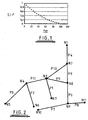
- the length weighted ICFs are them summed and divided by the total length of pipework within the network to give an average ICF for the network as a whole. This will now be illustrated by way of example with reference to Figure 2 which illustrates a simple pipe network.
- the pipe network of Figure 2 comprises 11 pipes, P1-P11, linking 11 nodes, N1-N11.
- Table 1 gives the ICF and length weighted ICF for each pipe P1-P11 calculated on the basis of the listed age and length data for each pipe and using the above empirical relationship (taking "Max Age” to be 110 years).
- the total leakage can be determined by conventional methods.
- the conventional method adopted for the purposes of exemplifying the invention is that mentioned above in which overall leakage is assumed to be proportional to the number of properties (houses) allocated to each node (or as appropriate the sum of the mains half-lengths either side of a node in a rural area).
- leakage rates will be referred to in terms of properties, the actual leakage values being directly proportional to the property values.
- Another aspect of the present invention provides a method of determining the most likely location, and size, of bursts within the network. Essentially, the invention provides a method of generating populations of burst distributions which can be compared with measured values using conventional hydraulic analysis techniques to arrive at a "best fit" population which closely matches the measured values. The "best fit" is preferably determined by comparison of the available or gauge pressures predicted by the network model to those measured at a sub-set of nodes used for calibration of the model and at which data loggers were used to accurately record pressures. The process is continued until successive generations of the predicted burst populations show no significant improvement in the best fit burst population.
- a first generation of populations of burst distributions (represented in the example by nodal property counts as mentioned above) is generated and the best fit population (i.e. burst distribution) is determined by hydraulic analysis (which may be entirely conventional). Certain information from the best fit population is then carried forward to a subsequent generation of populations to modify the generation of the burst distributions, i.e. to weight them towards the previous best fit. Hydraulic analysis is then performed on the second generation populations and the best fit population from that generation determined. The process is continued for third and subsequent generations until no significant improvement in the best fit population is made from one generation to the next. This best fit population is then taken as the solution.
- each population of burst distributions is generated, and tested, on the basis of the following basic steps:
- the best fit population is determined. This may for instance be determined by summing the differences between the measured pressure head values and those predicted on the basis of the burst distribution of a respective population, the best fit population being that with the lowest total difference.
- information from that population is carried over into at least some of the population members of a subsequent generation of burst populations. That is, information representing the relative sizes of the bursts allocated to nodes in accordance with the best fit population is used to weight the distribution of burst leakage amongst nodes in the generation of at least some of the burst populations of the subsequent generation.
- the distribution of burst leakage in each generation of burst populations is also weighted in accordance with a factor representative of the condition of each node.
- a factor representative of the condition of each node Preferably this is an average nodal ICF determined on the basis of individual pipe ICFs calculated as mentioned above.
- the weighting of the burst leakage distributions in the populations of a subsequent generation is then achieved (at least in part) by adjusting the ICF of appropriate nodes on the basis of the best fit information from the previous generation. That is, the nodal ICF value is adjusted to represent an increased likelihood of the existence of a burst, in proportion to the relative size of the burst allocated to that node in the previous generations best fit population.
- condition factor or modified condition factor (as the case may be), is used both to weight the initial allocation of bursts to nodes and the size of the burst allocated to a node.
- the objective is essentially to determine an allocation of bursts to nodes which a hydraulic analysis shows to be a close fit with the measured values.
- the likelihood and size of a burst appearing in a particular node is weighted in accordance with an average condition factor determined for that node.
- a preliminary step of the preferred method is to determine an average ICF for each node under consideration.
- to perform the hydraulic analysis on each population within each generation it is also necessary to distribute the total background leakage across the network. Whereas this may be done in accordance with conventional methods, a preferred method is provided by the present invention.
- the average nodal ICF is basically calculated in the same way as the average network ICF.
- the conventional method of apportioning background leakage across a network is to allocate background leakage to nodes within the network on the basis of demand associated with that each node.
- the demand at each node will typically be related to the number of houses with the node in a built up area and to the lengths or half lengths of pipes converging at a node in rural areas. Other basis for determining demand distribution may however be used.
- the particular method for associating demand with a node will depend on the particular network model used but whatever the method the demand distribution will be provided by the network model.
- a relatively simple conventional manner of distributing background leakage across a network would be to divide the total background leakage by the total demand to give an average background leakage per demand unit (e.g. average background leakage per property) and then to multiply the demand at each node by the average figure to give an absolute figure of the background leakage associated with that node. It will be appreciated from this calculation that the unit used in the demand allocation is not relevant in the final calculation.
- an average background leakage per demand unit e.g. average background leakage per property
- background leakage is related not only to the number of service connections (i.e. typically the number of houses) it is also related to the pipes themselves and the properties associated with those pipes, such as leaking pipe joints.
- the present invention accommodates the influence of background leakage from service pipes, thus improving upon the above method, by weighting the leakage associated with each node on the basis of the average nodal ICF of each node. This is done by dividing the demand allocated to a node by the average ICF of that node to obtain a factor which may be termed a "leakage factor".
- the amount of background per leakage LF for the network as a whole is then calculated by dividing the total background leakage by the total summed LFs for all nodes within the network.
- the leakage associated with any particular node is then simply calculated by multiplying that nodes LF by the background per LF figure.
- the LF for each node is first calculated by dividing that nodes demand allocation by its average ICF and then the leakage for each node is derived by dividing that nodes LF by the summed LFs for the whole network to give the fraction of the total leakage which may be associated with that node.
- the actual leakage value is then simply obtained by multiplying the total background leakage by this fraction.
- Table 3 shows the results of the LF and background leakage calculation for each node in the network of Figure 2 on the basis of a demand allocation (property counts) listed and on the basis of a total background leakage of 38.1 properties calculated above.
- Table 3 Node Av.ICF Demands LF Back.
- tables 4 and 5 below give the results of first and second generations of pipe burst populations generated on the basis of the network of Figure 2. In this simple example each generation comprises only three populations.
- the first row "order" sets out a randomly generated order in which the nodes will be considered.
- the second row, ''Fit'' sets out any weighting factor to be applied to each node on the basis of a best fit population from a previous generation. Since this is the first generation there is no weighting factor to be taken into account and thus the Fit for each node is zero.
- the third row gives the value "ICFm" for each node. This is the average ICF for each node calculated as described above but taking into account any modification made on the basis of the Fit information carried over from the previous generation. Again, since this is the first generation there is no fit information and thus in each case ICFm is the same as the original calculated ICF. Thus, the figures in this row are taken directly from table 2 above.
- a first random number, "random 1" is generated between 0 and 1 for each node.
- the number random1 for each node is then compared with the ICFm value for each node to create a pseudo-random population of burst leakage distributions.
- a "Y" is entered in the fifth row, "Is Leak", to designate that a burst has been assigned to that node.
- the ICF of a pipe and of a node gives an indication of the probability of a burst occurring at that pipe or node. The lower the ICF the greater the probability of a burst occurring. As the ICFm value tends to unity, that is the pipes around the node are in best condition, there is less likelihood that Random 1 will be greater than ICFm and thus less likelihood of a burst being allocated to a node.
- the generation of the burst leakage distribution indicated in the "Is leak" line is not entirely random as it takes into account the condition and thus likelihood of a burst occurring at any particular node. For instance, a node having a perfect ICF of 1 would never have a "Y" in the "Is Leak” column. Hence, the burst distribution is referred to as "pseudo-random".
- the ICFm for each burst node is subtracted from 1, the size of the remainder being directly indicative of the likelihood of a burst occurring at that node.
- the next step is to allocate the total burst leakage amongst the nodes.
- the first node for which a burst is indicated in the "Is Leak" row is considered first. In population 1a this is node N4.
- the total burst leakage for the network as a whole is then multiplied by the probability value "Prob" for node N4 to give the burst size at that node.
- the total burst leakage is taken to be that calculated earlier in this description, i.e. 11.92 litres per second (which is indicated in the final row of the population la identified as "remain” i.e. the remaining the burst leakage to be allocated).
- This is multiplied by the probability factor, 0.092 for N4 in this case, to give a burst leakage of 1.092 properties at N4 which is indicated in the eight row, "burst".
- the allocated burst leakage (1.092) is then subtracted from the total burst leakage figure of 11.924 to give a remainder of 10.831 litres per second burst leakage still to be allocated. This remainder appears in the "remain" row of the next node having a burst allocated to it, namely N2. Again this remaining figure is multiplied by the probability for that node, i.e. 0.203, to give a burst leakage of 2.195 litres per second at node N2.
- the burst leakage distribution suggested by population 1a is that indicated in the "burst" row.
- a conventional hydraulic analysis is then performed on the basis of this burst distribution, and on the basis of a distribution of background leakage which may be determined on a conventional basis but is preferably determined on the basis of the method described above, to determine the pressure head values that would be predicted to result from this distribution of leakage. These are then compared with measured values. A sum of the total differences between the predicted and measured values is then taken to be an indication of how well the burst distribution suggested by the population fits the measured data. In other words, the lower the difference the better the fit.
- a "fit" value is determined for each of the nodes of the best fit population. This is a number between 1 and 0 representing the proportion of total burst leakage allocated to each node in the best fit population.
- the fit value is 0 since no burst leakage was allocated to those nodes in the distribution of the best fit population 1b. The manner in which the fit value is used to influence the burst distributions allocated in the populations of the second generation will be described further below.
- the second way in which best fit information is carried over from one generation to the next is to carry over the node order from the best fit population. That is, N8, N6, N2, N5, N7, N4 and N3.
- the node order is exactly the same as that of the best fit population 1b from the first generation.
- the fit values calculated as mentioned above are indicated in the fit row. These fit values are used to influence the subsequent allocation of bursts by modifying the ICF of respective nodes. Specifically, the fit value is substrated from 1 and the remainder is used as a modifier which is multiplied together with the nodal ICF to give a modified ICF value indicated in the row "ICFm". Otherwise the procedure for generating the burst population is the same as for the first generation.
- bursts are weighted towards those nodes having bursts in the best fit population of the previous generation by reduction of the respective ICF values and that furthermore the weighting is related to the size of burst allocated to each node in the best fit population.
- Population 2b is generated in the same way as population 2a.
- Population 2c is generated in the same way as populations 2a and 2b except in this instance it will be noted that the node order is randomly generated rather than node carried over from the best fit of generation 1. This is done to introduce a random element into the process which reduces the likelihood of arriving at a solution which is effectively a local minima.
- a hydraulic analysis can then be performed on each population and the best fit selected under the criteria mentioned above.
- New fit values are generated on the basis of the second generation of the best fit population which are then carried over to a third generation together with a best fit node order.
- Third and subsequent generations can then be generated on the same basis as the second generation until no significant improvement is found from one generation to the next in the fit of the best fit burst allocations.
- the final best fit population is then taken as the solution.
- the random numbers "random 1" and “random 2" are calculated between 0 and 1 since this is the full range of possible ICFs in accordance with the calculation made earlier in the description. It is of course entirely possible that the ICF range differs from that used in this example and thus that the random ranges will differ accordingly. It will also be readily apparent that the precise arithmetic operations may vary. For instance, ICF values may be established on a different basis from that used above. For example, ICF values could be calculated on a basis which gives a low ICF for a pipe in good condition with low burst probability.
- ICF values could also be modified to take account of the certainty or otherwise of the information used to generate those values. For instance the age of a particular pipe might not be known in which case it might be necessary to estimate the age, perhaps on the basis of the age of a related node. Each ICF could therefore be multiplied by a probability factor (eg between 0 and 1) based on the expected accuracy of the information used to calculate the ICF.
- a probability factor eg between 0 and 1
- the burst allocation process could be run without any modification based on ICF values.
- the burst leakage allocation in the first generation of populations could be generated on a purely random basis and best fit information carried over to subsequent generations and used to modify the random number elements such as random 1 and random 2.
- Use of ICF values is however a much preferred method as it gives a systematic weighting taking into account the condition of pipe work.
- the calculation of the probability factor "Prob" could be made purely on the basis of the ICF value rather than the ICF value as modified by a randomly generated number (random 2).
- the residual burst leakage remaining after allocation has been made to all nodes in a population deemed to have a burst could be made in a different manner from that described.
- the residual burst is allocated to a single node but could for instance be split between all nodes not already allocated with a burst.
- the random element introduced into each generation can vary.
- one population out of three in the second and subsequent generations is based on a new random pipe order (although including fit values from the previous generation best fit population). This ratio could vary.
- random solutions could be introduced by including populations in second and subsequent generations that do not take account of the fit information.
- a further aspect of the present invention is that once burst and background leakage has been allocated in accordance with the preferred methods described above, calibration of the network model as a whole is improved over that achieved using conventional techniques. Thus, ultimately the present invention provides a method which provides improved calibration of a pipe network model.
- the various aspects of the present invention need not necessarily be combined.
- the burst allocation method could be used in conjunction with alternative methods of determining the overall volumes of burst leakage and allocation of background leakage.
- the preferred methods for determining the ratio of background to burst leakage could be used in other methods of identifying individual bursts.
- the proposed method representing the likelihood of any given pipe experiencing a burst by generation of ICF values could be used in other methods of calibrating a pipe network.
- the various aspects of the present invention are particularly advantageous when used together but could nevertheless be used independently in conjunction with other conventional methods.
Landscapes
- Engineering & Computer Science (AREA)
- Mechanical Engineering (AREA)
- General Engineering & Computer Science (AREA)
- Pipeline Systems (AREA)
- Examining Or Testing Airtightness (AREA)
- Management, Administration, Business Operations System, And Electronic Commerce (AREA)
- Data Exchanges In Wide-Area Networks (AREA)
- Complex Calculations (AREA)
- Sink And Installation For Waste Water (AREA)
Claims (28)
- Verfahren zum Unterteilen der Gasamtleckageverluste eines Rohrnetzwerkes in Hintergrundeigenleckage und Bruchleckage, wobei das Verfahren die folgenden Schritte umfasst:Definieren eines ersten Infrastrukturzustandsfaktors (ICF), der eine numerische Darstellung des Zustands eines Netzwerkes in einem Gut-Schwellenzustand ist, in dem Hintergrundeigenleckage als ein vernachlässigbarer Anteil des Netzwerk-Gesamtleckageverlustes angenommen werden kann;Definieren eines zweiten ICF, der eine numerische Darstellung des Zustands eines Netzwerkes in einem Schlecht-Schwellenzustand ist, in dem die Gesamtleckageverluste von Hintergrundei genleckage dominiert werden;Ableiten eines Netzwerk-ICF für das betrachtete Netzwerk, das den Zustand des Netzwerkes als numerischen Bruchteil der Differenz zwischen dem ersten und dem zweiten ICF ausdrückt;Ermitteln der Gesamtleckageverluste von dem Netzwerk durch Ausführen einer Netzwerkanalyse an dem Netzwerk;und Multiplizieren der Gesamtleckageverluste mit dem Netzwerk-ICF, um die Gesamtleckageverluste in Hintergrundeigenleckage und Gesamtnetzwerkbruchleckage zu unterteilen.
- Verfahren nach Anspruch 1, bei dem der Gesamtleckageverlust mit dem Nctzwerk-ICF multipliziert wird, so dass direkt das Niveau an Bruch- oder Hintergrundleckage jeweils in Abhängigkeit davon erhalten wird, ob der erste ICF als höher als der zweite ICF oder umgekehrt definiert ist, wobei der Rest jeweils als Hintergrund- oder Bruchlenkage angenommen wird.
- Verfahren nach Anspruch 1 oder Anspruch 2, wobei der Netzwerk-ICF durch Ermitteln eines Rohr-ICF für jedes Rohr in dem Netzwerkmodell, das ein numerischer Ausdruck der erwarteten proportionalen. Unterteilung von Leckage in Hintergrundleckage und Bruchleckage in einem theoretischen Netzwerk ist, das Rohre umfasst, die alle diesen ICF haben, und Mitteln der Rohr-ICF-Werte über das Netzwerk, so dass sich der Netzwerk-ICF ergibt.
- Verfahren nach Anspruch 3, wobei die Mittelwertbildung durchgeführt wird durch eine erste Längengewichtung jedes der Rohr-ICFs durch Multiplizieren jedes Rohr-ICF mit der Länge des jeweiligen Rohres, Summieren der längengewichteten Rohr-ICFs aller Rohre in dem Netzwerk und Dividieren der Summe der längengewichteten Rohr-ICFs durch die Rohrgesamtlänge in dem Netzwerk, um den Netzwerk-ICF zu erhalten.
- Verfahren nach Anspruch 4, wobei der Rohr-ICF jedes einzelnen Rohres in dem Netzwerk abgeleitet wird auf empirischer als Funktion von einem oder mehreren aus Alter, Material, Anzahl der Rohrverbindungen und -anschlüsse, und Bodenbedingungen, die dem jeweiligen Rohr zuzuordnen sind.
- Verfahren nach einem der vorherigen Ansprüche, das ferner das Ermitteln der wahrscheinlichsten Größe und Stelle eines Bruchs im Rohrnetzwerk umfasst, durch:Erzeugen einer ersten Generation von Bruchpopulationen, in denen jeweils die Gesamtbruchlcckage zwischen Knoten des Netzwerkmodells verteilt ist;Durchführen einer Netzwerkanalyse an dem Netzwerkmodell für jede der Bruchpopulationen, wobei die Netzwerkanalyse in jedem Fall auf der Basis der jeweiligen Verteilung von Brüchen über das Netzwerk erfolgt;Vergleichen von Betriebsparametern des Netzwerkes, die durch Netzwerkanalyse für jede Bruchpopulation mit Messwerten der Betriebsparameter ermittelt werden, um eine Best-Fit-Bruchpopulation zu ermitteln, für welche die mit der Netzwerkanalyse ermittelten Betriebsparameterwerte am besten mit den Messwerten übereinstimmen;Erzeugen zweiter und nachfolgender Generation(en) von Bruchpopulationen, wobei die Verteilung von Brüchen in wenigstens einigen der Bruchpopulationen jeder Generation gemäß der Bruchverteilung der Best-Fit-Population der vorherigen Bruchgeneration gewichtet wird;Ausführen der Netzwerkanalyse und des Best-Fit-Vergleichs an jeder Generation und Fortsetzen, bis nachfolgende Generationen keine erhebliche Verbesserung der Best-Fit-Bruchpopulation mehr zeigen.
- Verfahren nach Anspruch 6, bei dem wenigstens einige der Bruchpopulationen der zweiten und jeder nachfolgenden Generation von Bruchpopulationen ohne Gewichtung gemäß der vorherigen Best-Fit-Bruchpopulation erzeugt werden.
- Verfahren nach Anspruch 6 oder Anspruch 7, wobei die Verteilung der Gesamtbruchleckage innerhalb jeder Bruchpopulation jeder Generation gemäß einem Knotens-Infrastrukturzustandsfaktor (ICF) gewichtet wird, der für den relativen Zustand jedes Knotens repräsentativ und für die Wahrscheinlichkeit indikativ ist, dass ein Bruch mit diesem Knoten assoziiert ist.
- Verfahren nach Anspruch 8, wobei der Knoten-ICF jedes Knotens im Netzwerk durch Dividieren der Summe der längengewichteten ICFs jedes Rohres, das am jeweiligen Knoten konvergiert, durch die Gesamtlänge der an diesem Knoten konvergierenden Rohre ermittelt wird.
- Verfahren nach Anspruch 8 oder Anspruch 9, wobei die Verteilung der Gesamtbruchleckage innerhalb jeder Bruchpopulation gemäß dem Knoten-ICF durch folgende Prozedur gewichtet wird:Erzeugen einer ersten Zufallszahl für jeden Knoten, die innerhalb des Bereiches der möglichen Knoten-ICF-Werte liegt;Vergleichen der ersten ZuFallszahl mit dem ICF des jeweiligen Knotens und Zuordnen eines Bruchs zu diesem Knoten, wenn die erste Zufallszahl größer oder kleiner als der ICF ist, je nach dem, ob die ICF-Werte so definiert sind, dass höhere Werte einen besseren Netzwerkzustand repräsentieren oder umgekehrt.
- Verfahren nach Anspruch 10, wobei der Knoten-ICF zur Gewichtung sowohl der Verteilung von Brüchen über Knotene in einer bestimmten Bruchpopulation als auch der Größe von Brüchen verwendet wird, die jedem Knoten dieser Population zugeordnet sind.
- Verfahren nach Anspruch 11, wobei die Größe von Brüchen, die bestimmten Knoten zugeordnet werden, durch folgende Prozedur ermittelt wird:Multiplizieren der Differenz zwischen dem Knoten-ICF eines jeweiligen Knotens und dem maximalen für einen Knoten möglichen ICF durch eine zweite Zufallszahl zwischen 0 und 1, um einen Bruchwahrscheinlichkeitsfaktor zu definieren;Berücksichtigen eines ersten Knotens, dem ein Bruch zugeordnet wurde, und Multiplizieren der Gesamtbruchleckage für das Netzwerk mit dem für diesen Knoten abgeleiteten Wahrscheinlichkeitsfaktor, um die Größe des Bruchs zu ermitteln, die für diesen Knoten zuzuordnen ist;Berücksichtigen eines zweiten Knotens, dem ein Bruch zugeordnet wurde, und Multiplizieren der unzugeordneten Restbruchleckage mit dem Bruchwahrscheinlichkeitsfaktor dieses Knoten, um die diesem Knoten zuzuordnende Bruchgröße zu ermitteln;Wiederholen des obigen Vorgangs für jeden Knoten, dem ein Bruch zugeordnet wurde, bis die Größe der zugeordneten Brüche für alle solche Knotene ermittelt ist; undzufallsmäßiges Zuordnen der unzugeordncten Restbruchleckage zu wenigstens einem der Knotene, dem nicht ursprünglich ein Bruch zugeordnet wurde.
- Verfahren nach Anspruch 12, wobei die Reihenfolge, in der die Knotene zur Ermittlung von Bruchgrößen berücksichtigt werden, zufallsmäßig für wenigstens einige Populationen jeder Generation von Populationen ermittelt wird.
- Verfahren nach einem der Ansprüche 8 bis 13, wobei die Gewichtung der Bruchverteilung innerhalb von Bruchpopulationen der zweiten und nachfolgender Generation(en) auf der Basis der vorherigen Best-Fit-Bruchpopulation erzielt wird durch Modifizieren des Knoten-ICF jedes Knotens innerhalb einer Population gemäß der relativen Verteilung von Brüchen über jeweilige Knotene der vorherigen Best-Fit-Population.
- Verfahren nach Anspruch 14, wobei ein Fit-Wert für jeden Knoten, dem ein Bruch in der vorherigen Best-Fit-Bruchpopulation zugeordnet wurde, durch Dividieren der einem bestimmten Knoten zugeordneten Bruchleckage durch die Gesamtbruchleckage für das Netzwerk und Modifizieren des ICF eines jeweiligen Knotens als Funktion des Fit-Wertes abgeleitet wird.
- Verfahren nach Anspruch 15, wobei der Fit-Wert für einen Knoten von Eins subtrahiert und der Rest als Modifizierer verwendet wird, der zusammen mit dem Knoten-ICF des jeweiligen Knotens multipliziert wird, so dass sich ein modifizierter ICF für diesen Knoten ergibt, wobei der modifizierte ICF anstelle des ursprünglichen ICF in den nachfolgenden Bruchzuordnungsprozeduren verwendet wird.
- Verfahren nach einem der Ansprüche 12 bis 16, wobei die Reihenfolge, in der Knotene zur Ermittlung von Bruchgrößen für wenigstens einige der Bruchpopulationen der zweiten und nachfolgender Generation(en) berücksichtigt werden, der Reihenfolge von Knoten von der vorherigen Best-Fit-Population entspricht.
- Verfahren nach einem der Ansprüche 8 bis 17, wobei beim Ausführen der Netzwerkanalyse die Gesamthintergrundleckage zwischen Knoten des Netzwerkes verteilt wird.
- Verfahren nach Anspruch 18, wobei die Hintergrundleckage Knoten des Netzwerkes als Funktion der Benutzeranfrage an jedem Knoten des Netzwerkes zugeordnet wird.
- Verfahren nach Anspruch 19, wobei die Gesamthintergrundleckage Knoten des Netzwerkes folgendermaßen zugeordnet wird:Dividieren der mit dem Knoten assoziierten Anfrage durch den Knoten-ICF, um einen Knotensleckagefaktor (LF) abzuleiten;Multiplizieren des Knotens-LF mit der Gesamthintergrundleckage für das Netzwerk und Dividieren durch die Summe der Knotens-LFs aller Knoten in dem Netzwerk.
- Verfahren zum Kalibrieren eines RohrNetzwerkmodells durch Ermitteln der Bruch- und Hintergrundleckageverteilung nach einem der vorherigen Ansprüche.
- Verfahren zum Ermitteln der wahrscheinlichsten Größe und Stelle von Brüchen in einem RohrNetzwerk, wobei das Verfahren folgendes umfasst:Ermitteln der mit dem Netzwerk assoziierten Gesamtbruchleckage durch eine Netzwerkanalyse an einem Modell des Netzwerkes;Erzeugen einer ersten Generation von Bruchpopulationen, in denen die Gesamtbruchleckage zwischen Knoten des Netzwerkmodells verteilt ist;Durchführen einer Netrwerkanalyse an dem Netzwerkmodell für jede der Bruchpopulationen, wobei die Netzwerkanalyse in jedem Fall auf der Basis der jeweiligen Verteilung von Brüchen über das Netzwerk durchgeführt wird;Vergleichen von Betriebsparametern des Netzwerkes, die durch die Netzwerkanalyse für jede Bruchpopulation ermittelt wurden, mit Messwerten der Betriebsparameter, um eine Best-Fit-Bruchpopulation zu ermitteln, für welche die durch die Netzwerkanalyse ermittelten Betriebsparameterwerte am besten mit den Messwerten übereinstimmen;Erzeugen zweiter und nachfolgender Generation(en) von Bruchpopulationen, wobei die Verteilung von Brüchen in wenigstens einigen der Bruchpopulationen jeder Generation gemäß der Bruchverteilung der Best-Fit-Population der vorherigen Bruchgencration gewichtet wird;Durchführen der Netzwerkanalyse und des Best-Fit-Vergleichs an jeder Generation und Fortsetzen, bis nachfolgende Generationen keine signifikante Verbesserung der Best-Fit-Bmchpopulation mehr zeigen.
- Verfahren nach Anspruch 22, das ferner Merkmale aus beliebigen der Ansprüche 7 bis 20 umfasst.
- Verfahren zum Zuordnen von Hintergrundeigenleckagen über die Knotene eines RohrNetzwerkmodells, das folgendes umfasst:Ermitteln der Gesamthintergrundleckage des Netzwerkes;Ermitteln der Benutzeranfrage an jedem Knoten des Netzwerkes;Ermitteln eines Knotens-Infrastrukturzustandsfaktors (ICF) für jeden Knoten, der den relativen Zustand jedes Knotens repräsentiert;Dividieren der mit jedem Knoten assoziierten Anfrage durch den Knoten-ICF dieses Knotens, um einen Knotensleckfaktor (LF) abzuleiten;und Multiplizieren des Knotens-LF mit der Gesamthintergrundleckage für das Netzwerk und Dividieren durch die Summe der Knotens-LFs aller Knotene in dem Netzwerk, um die Hintergrundleckage zu ermitteln, die diesem Knoten zuzuordnen ist.
- Verfahren nach Anspruch 24, wobei die Knoten-ICF-Werte durch Ermitteln eines Rohr-ICF für jedes Rohr in dem Netzwerkmodell abgeleitet werden, das ein numerischer Ausdruck der erwarteten proportionalen Unterteilung von Leckage in Hintergrundleckage und Bruchleckage in einem theoretischen Netzwerk ist, das Rohre umfasst, die alle diesen ICF haben, Längsgewichtung jedes der Rohr-ICFs durch Multiplizieren jedes Rohr-ICF mit der Länge des jeweiligen Rohrs, und Dividieren der Summe von längsgewichteten ICFs jedes am jeweiligen Knoten konvergierenden Rohrs durch die Gesamtlänge der an diesem Knoten konvergierenden Rohre.
- Verfahren nach Anspruch 25, wobei der Rohr-ICF jedes einzelnen Rohrs in dem Netzwerk abgeleitet wird auf empirischer Basis als Funktion von einem oder mehreren von Alter, Material, Anzahl der Rohrverbindungen und -anschlüsse, und Bodenbedingungen, die dem jeweiligen Rohr zuzuordnen sind.
- Computerprogramm zum Ausführen eines Verfahrens nach einem der vorherigen Ansprüche.
- Trägermedium, das rechnerlesbaren Code trägt, um einen Computer zu veranlassen, eine Prozedur gemäß dem Verfahren nach einem der Ansprüche 1 bis 26 auszuführen.
Applications Claiming Priority (3)
| Application Number | Priority Date | Filing Date | Title |
|---|---|---|---|
| GB0105183 | 2001-03-01 | ||
| GBGB0105183.8A GB0105183D0 (en) | 2001-03-01 | 2001-03-01 | Determination of leakage and identification of bursts in a pipe network |
| PCT/GB2002/000869 WO2002070945A1 (en) | 2001-03-01 | 2002-03-01 | Determination of leakage and identification of bursts in a pipe network |
Publications (2)
| Publication Number | Publication Date |
|---|---|
| EP1364154A1 EP1364154A1 (de) | 2003-11-26 |
| EP1364154B1 true EP1364154B1 (de) | 2006-06-07 |
Family
ID=9909852
Family Applications (1)
| Application Number | Title | Priority Date | Filing Date |
|---|---|---|---|
| EP02701435A Expired - Lifetime EP1364154B1 (de) | 2001-03-01 | 2002-03-01 | Verfahren zur erkennung und ortung von leckagen in rohrleitungen |
Country Status (12)
| Country | Link |
|---|---|
| US (1) | US20040148113A1 (de) |
| EP (1) | EP1364154B1 (de) |
| AT (1) | ATE329201T1 (de) |
| BG (1) | BG108156A (de) |
| CZ (1) | CZ20032530A3 (de) |
| DE (1) | DE60212081D1 (de) |
| EE (1) | EE200200619A (de) |
| GB (1) | GB0105183D0 (de) |
| HU (1) | HUP0302164A3 (de) |
| RU (1) | RU2003126603A (de) |
| SK (1) | SK10822003A3 (de) |
| WO (1) | WO2002070945A1 (de) |
Families Citing this family (12)
| Publication number | Priority date | Publication date | Assignee | Title |
|---|---|---|---|---|
| FR2915755B1 (fr) * | 2007-05-04 | 2011-04-29 | Suez Environnement | Procede et installation de controle en temps reel de la qualite de l'eau d'un reseau de distribution. |
| US9053519B2 (en) * | 2012-02-13 | 2015-06-09 | TaKaDu Ltd. | System and method for analyzing GIS data to improve operation and monitoring of water distribution networks |
| US10242414B2 (en) * | 2012-06-12 | 2019-03-26 | TaKaDu Ltd. | Method for locating a leak in a fluid network |
| US10203262B2 (en) | 2014-02-19 | 2019-02-12 | Tata Consultancy Services Limited | Leak localization in water distribution networks |
| US10380272B2 (en) * | 2015-04-30 | 2019-08-13 | International Business Machines Corporation | Update computer-implemented method, computer program product and computer system for generating or updating topology model of pressure pipe network |
| EP3327206B1 (de) * | 2016-11-25 | 2020-03-25 | Tata Consultancy Services Limited | Klassifizierung von rohren zur wartung in leitungsnetzen unter verwendung ungefährer hydraulischer metriken |
| CN111832793A (zh) * | 2020-01-10 | 2020-10-27 | 吉林建筑大学 | 一种基于管网突发性污染事件的污染源定位方法及系统 |
| CN113405026B (zh) * | 2020-03-16 | 2022-11-11 | 中国港湾工程有限责任公司 | 一种适用于欠发达地区供水管网的新增漏损判别及其漏损率的估算方法 |
| CN113883423B (zh) * | 2021-10-19 | 2023-02-07 | 山东腾威石油装备有限公司 | 一种新型管网修复加强方法 |
| CN114357679A (zh) * | 2022-01-05 | 2022-04-15 | 烟台杰瑞石油服务集团股份有限公司 | 高压管汇运行状态的处理方法以及装置 |
| CN114580786B (zh) * | 2022-03-30 | 2024-11-12 | 广州市自来水有限公司 | 一种用于城市供水管网监测点的布置优化方法 |
| CN118623242B (zh) * | 2024-08-15 | 2024-11-08 | 南通西屋智能科技有限公司 | 一种基于供水管网的dma区域漏损监测管理方法及系统 |
Family Cites Families (11)
| Publication number | Priority date | Publication date | Assignee | Title |
|---|---|---|---|---|
| US3695094A (en) * | 1970-07-16 | 1972-10-03 | Halliburton Co | Leak detection method and system |
| US3667285A (en) * | 1970-08-18 | 1972-06-06 | Customline Control Products In | Leak detection system |
| SU766210A1 (ru) * | 1979-05-31 | 1982-04-30 | Проектный Институт "Коммуналпроект" | Способ дистанционного определени места повреждени в напорной трубопроводной сети |
| DE3909337A1 (de) * | 1989-03-22 | 1990-09-27 | Sewerin Hermann Gmbh | Verfahren und vorrichtung zur ueberpruefung von unterirdisch verlegten, gas oder fluessigkeit fuehrenden rohren auf undichtigkeit |
| US5272646A (en) * | 1991-04-11 | 1993-12-21 | Farmer Edward J | Method for locating leaks in a fluid pipeline and apparatus therefore |
| JP3543426B2 (ja) * | 1995-07-06 | 2004-07-14 | 株式会社日立製作所 | 管路網管理方法およびシステム |
| DE19542890C1 (de) * | 1995-11-17 | 1997-07-17 | Hansaconsult Ingenieurgesellsc | Verfahren zur Erkennung von Leckagen in Rohrleitungen |
| DE19701317A1 (de) * | 1997-01-16 | 1998-07-23 | Peter Dipl Ing Renner | Leckerkennung in Rohrleitungssystemen |
| US5974862A (en) * | 1997-05-06 | 1999-11-02 | Flow Metrix, Inc. | Method for detecting leaks in pipelines |
| US6535827B1 (en) * | 1999-10-28 | 2003-03-18 | Mpr Associates, Inc. | Method and apparatus for detecting and isolating a rupture in fluid distribution system |
| JP4314038B2 (ja) * | 2002-11-08 | 2009-08-12 | エネジン株式会社 | 流体搬送管網中の異常箇所を推定する方法 |
-
2001
- 2001-03-01 GB GBGB0105183.8A patent/GB0105183D0/en not_active Ceased
-
2002
- 2002-03-01 EP EP02701435A patent/EP1364154B1/de not_active Expired - Lifetime
- 2002-03-01 HU HU0302164A patent/HUP0302164A3/hu unknown
- 2002-03-01 SK SK10822003A patent/SK10822003A3/sk unknown
- 2002-03-01 EE EEP200200619A patent/EE200200619A/xx unknown
- 2002-03-01 WO PCT/GB2002/000869 patent/WO2002070945A1/en not_active Ceased
- 2002-03-01 RU RU2003126603/06A patent/RU2003126603A/ru not_active Application Discontinuation
- 2002-03-01 CZ CZ20032530A patent/CZ20032530A3/cs unknown
- 2002-03-01 US US10/469,320 patent/US20040148113A1/en not_active Abandoned
- 2002-03-01 DE DE60212081T patent/DE60212081D1/de not_active Expired - Lifetime
- 2002-03-01 AT AT02701435T patent/ATE329201T1/de not_active IP Right Cessation
-
2003
- 2003-09-04 BG BG108156A patent/BG108156A/xx unknown
Also Published As
| Publication number | Publication date |
|---|---|
| GB0105183D0 (en) | 2001-04-18 |
| HUP0302164A3 (en) | 2005-10-28 |
| ATE329201T1 (de) | 2006-06-15 |
| EP1364154A1 (de) | 2003-11-26 |
| HUP0302164A2 (hu) | 2003-10-28 |
| US20040148113A1 (en) | 2004-07-29 |
| DE60212081D1 (de) | 2006-07-20 |
| CZ20032530A3 (cs) | 2004-06-16 |
| SK10822003A3 (en) | 2004-10-05 |
| WO2002070945A1 (en) | 2002-09-12 |
| BG108156A (en) | 2004-04-30 |
| RU2003126603A (ru) | 2005-02-20 |
| EE200200619A (et) | 2004-06-15 |
Similar Documents
| Publication | Publication Date | Title |
|---|---|---|
| EP1364154B1 (de) | Verfahren zur erkennung und ortung von leckagen in rohrleitungen | |
| Wu et al. | Water loss detection via genetic algorithm optimization-based model calibration | |
| Berardi et al. | Calibration of design models for leakage management of water distribution networks | |
| Tabesh et al. | An integrated model to evaluate losses in water distribution systems | |
| Wagner et al. | Water distribution reliability: Simulation methods | |
| V ı´ tkovský et al. | Optimal measurement site locations for inverse transient analysis in pipe networks | |
| US8175859B1 (en) | Efficient method for pressure dependent water distribution analysis | |
| Steffelbauer et al. | Sensor placement and leakage localization considering demand uncertainties | |
| Cobacho et al. | Including leakage in network models: an application to calibrate leak valves in EPANET | |
| Lambert et al. | Using practical predictions of economic intervention frequency to calculate short-run economic leakage level, with or without pressure management | |
| CN108332059A (zh) | 服务于供水管网爆管监测的测压点优化布置方法 | |
| AU2017344456A1 (en) | Pipe leak measurement and assessment | |
| Martínez-Solano et al. | Exact skeletonization method in water distribution systems for hydraulic and quality models | |
| Lipiwattanakarn et al. | Water quality audit in drinking water distribution networks | |
| Chang et al. | Quantification of the head-outflow relationship for pressure-driven analysis in water distribution networks | |
| Okeya et al. | Locating pipe bursts in a district metered area via online hydraulic modelling | |
| Boatwright et al. | Optimal sensor placement and leak/burst localisation in a water distribution system using spatially-constrained inverse-distance weighted interpolation | |
| Berardi et al. | Feasibility of mass balance approach to water distribution network model calibration | |
| Gomes et al. | Efficiency indicator for assessment of water distribution networks carrying capacity | |
| CN113255125A (zh) | 一种基于多目标预测模型的供水管网失效更新策略方法 | |
| Amoatey et al. | Impact of active night population and leakage exponent on leakage estimation in developing countries | |
| CN107677343A (zh) | 一种智能水表运行误差远程校准方法 | |
| Ferreira et al. | Leak detection and location in a real water distribution network using a model-based technique | |
| CN108122074B (zh) | 一种给水管网模型中漏失水量的分配方法 | |
| Park et al. | Hydraulic power capacity of water distribution networks in uncertain conditions of deterioration |
Legal Events
| Date | Code | Title | Description |
|---|---|---|---|
| PUAI | Public reference made under article 153(3) epc to a published international application that has entered the european phase |
Free format text: ORIGINAL CODE: 0009012 |
|
| 17P | Request for examination filed |
Effective date: 20030901 |
|
| AK | Designated contracting states |
Kind code of ref document: A1 Designated state(s): AT BE CH CY DE DK ES FI FR GB GR IE IT LI LU MC NL PT SE TR |
|
| AX | Request for extension of the european patent |
Extension state: AL LT LV MK RO SI |
|
| 17Q | First examination report despatched |
Effective date: 20041104 |
|
| GRAP | Despatch of communication of intention to grant a patent |
Free format text: ORIGINAL CODE: EPIDOSNIGR1 |
|
| GRAS | Grant fee paid |
Free format text: ORIGINAL CODE: EPIDOSNIGR3 |
|
| GRAA | (expected) grant |
Free format text: ORIGINAL CODE: 0009210 |
|
| AK | Designated contracting states |
Kind code of ref document: B1 Designated state(s): AT BE CH CY DE DK ES FI FR GB GR IE IT LI LU MC NL PT SE TR |
|
| AX | Request for extension of the european patent |
Extension state: AL LT LV MK RO SI |
|
| PG25 | Lapsed in a contracting state [announced via postgrant information from national office to epo] |
Ref country code: IT Free format text: LAPSE BECAUSE OF FAILURE TO SUBMIT A TRANSLATION OF THE DESCRIPTION OR TO PAY THE FEE WITHIN THE PRESCRIBED TIME-LIMIT;WARNING: LAPSES OF ITALIAN PATENTS WITH EFFECTIVE DATE BEFORE 2007 MAY HAVE OCCURRED AT ANY TIME BEFORE 2007. THE CORRECT EFFECTIVE DATE MAY BE DIFFERENT FROM THE ONE RECORDED. Effective date: 20060607 Ref country code: NL Free format text: LAPSE BECAUSE OF FAILURE TO SUBMIT A TRANSLATION OF THE DESCRIPTION OR TO PAY THE FEE WITHIN THE PRESCRIBED TIME-LIMIT Effective date: 20060607 Ref country code: FI Free format text: LAPSE BECAUSE OF FAILURE TO SUBMIT A TRANSLATION OF THE DESCRIPTION OR TO PAY THE FEE WITHIN THE PRESCRIBED TIME-LIMIT Effective date: 20060607 Ref country code: BE Free format text: LAPSE BECAUSE OF FAILURE TO SUBMIT A TRANSLATION OF THE DESCRIPTION OR TO PAY THE FEE WITHIN THE PRESCRIBED TIME-LIMIT Effective date: 20060607 Ref country code: CH Free format text: LAPSE BECAUSE OF FAILURE TO SUBMIT A TRANSLATION OF THE DESCRIPTION OR TO PAY THE FEE WITHIN THE PRESCRIBED TIME-LIMIT Effective date: 20060607 Ref country code: LI Free format text: LAPSE BECAUSE OF FAILURE TO SUBMIT A TRANSLATION OF THE DESCRIPTION OR TO PAY THE FEE WITHIN THE PRESCRIBED TIME-LIMIT Effective date: 20060607 Ref country code: AT Free format text: LAPSE BECAUSE OF FAILURE TO SUBMIT A TRANSLATION OF THE DESCRIPTION OR TO PAY THE FEE WITHIN THE PRESCRIBED TIME-LIMIT Effective date: 20060607 |
|
| REG | Reference to a national code |
Ref country code: GB Ref legal event code: FG4D |
|
| REG | Reference to a national code |
Ref country code: CH Ref legal event code: EP |
|
| REG | Reference to a national code |
Ref country code: IE Ref legal event code: FG4D |
|
| REF | Corresponds to: |
Ref document number: 60212081 Country of ref document: DE Date of ref document: 20060720 Kind code of ref document: P |
|
| PG25 | Lapsed in a contracting state [announced via postgrant information from national office to epo] |
Ref country code: SE Free format text: LAPSE BECAUSE OF FAILURE TO SUBMIT A TRANSLATION OF THE DESCRIPTION OR TO PAY THE FEE WITHIN THE PRESCRIBED TIME-LIMIT Effective date: 20060907 Ref country code: DK Free format text: LAPSE BECAUSE OF FAILURE TO SUBMIT A TRANSLATION OF THE DESCRIPTION OR TO PAY THE FEE WITHIN THE PRESCRIBED TIME-LIMIT Effective date: 20060907 |
|
| PG25 | Lapsed in a contracting state [announced via postgrant information from national office to epo] |
Ref country code: DE Free format text: LAPSE BECAUSE OF FAILURE TO SUBMIT A TRANSLATION OF THE DESCRIPTION OR TO PAY THE FEE WITHIN THE PRESCRIBED TIME-LIMIT Effective date: 20060908 |
|
| PG25 | Lapsed in a contracting state [announced via postgrant information from national office to epo] |
Ref country code: ES Free format text: LAPSE BECAUSE OF FAILURE TO SUBMIT A TRANSLATION OF THE DESCRIPTION OR TO PAY THE FEE WITHIN THE PRESCRIBED TIME-LIMIT Effective date: 20060918 |
|
| PG25 | Lapsed in a contracting state [announced via postgrant information from national office to epo] |
Ref country code: PT Free format text: LAPSE BECAUSE OF FAILURE TO SUBMIT A TRANSLATION OF THE DESCRIPTION OR TO PAY THE FEE WITHIN THE PRESCRIBED TIME-LIMIT Effective date: 20061107 |
|
| LTIE | Lt: invalidation of european patent or patent extension |
Effective date: 20060607 |
|
| NLV1 | Nl: lapsed or annulled due to failure to fulfill the requirements of art. 29p and 29m of the patents act | ||
| REG | Reference to a national code |
Ref country code: CH Ref legal event code: PL |
|
| PLBE | No opposition filed within time limit |
Free format text: ORIGINAL CODE: 0009261 |
|
| STAA | Information on the status of an ep patent application or granted ep patent |
Free format text: STATUS: NO OPPOSITION FILED WITHIN TIME LIMIT |
|
| EN | Fr: translation not filed | ||
| 26N | No opposition filed |
Effective date: 20070308 |
|
| PG25 | Lapsed in a contracting state [announced via postgrant information from national office to epo] |
Ref country code: MC Free format text: LAPSE BECAUSE OF NON-PAYMENT OF DUE FEES Effective date: 20070331 Ref country code: IE Free format text: LAPSE BECAUSE OF NON-PAYMENT OF DUE FEES Effective date: 20070301 |
|
| PG25 | Lapsed in a contracting state [announced via postgrant information from national office to epo] |
Ref country code: GR Free format text: LAPSE BECAUSE OF FAILURE TO SUBMIT A TRANSLATION OF THE DESCRIPTION OR TO PAY THE FEE WITHIN THE PRESCRIBED TIME-LIMIT Effective date: 20060908 Ref country code: FR Free format text: LAPSE BECAUSE OF FAILURE TO SUBMIT A TRANSLATION OF THE DESCRIPTION OR TO PAY THE FEE WITHIN THE PRESCRIBED TIME-LIMIT Effective date: 20070309 |
|
| PG25 | Lapsed in a contracting state [announced via postgrant information from national office to epo] |
Ref country code: FR Free format text: LAPSE BECAUSE OF FAILURE TO SUBMIT A TRANSLATION OF THE DESCRIPTION OR TO PAY THE FEE WITHIN THE PRESCRIBED TIME-LIMIT Effective date: 20060607 |
|
| PG25 | Lapsed in a contracting state [announced via postgrant information from national office to epo] |
Ref country code: CY Free format text: LAPSE BECAUSE OF FAILURE TO SUBMIT A TRANSLATION OF THE DESCRIPTION OR TO PAY THE FEE WITHIN THE PRESCRIBED TIME-LIMIT Effective date: 20060607 Ref country code: LU Free format text: LAPSE BECAUSE OF NON-PAYMENT OF DUE FEES Effective date: 20070301 |
|
| PG25 | Lapsed in a contracting state [announced via postgrant information from national office to epo] |
Ref country code: TR Free format text: LAPSE BECAUSE OF FAILURE TO SUBMIT A TRANSLATION OF THE DESCRIPTION OR TO PAY THE FEE WITHIN THE PRESCRIBED TIME-LIMIT Effective date: 20060607 |
|
| PGFP | Annual fee paid to national office [announced via postgrant information from national office to epo] |
Ref country code: GB Payment date: 20130228 Year of fee payment: 12 |
|
| GBPC | Gb: european patent ceased through non-payment of renewal fee |
Effective date: 20140301 |
|
| PG25 | Lapsed in a contracting state [announced via postgrant information from national office to epo] |
Ref country code: GB Free format text: LAPSE BECAUSE OF NON-PAYMENT OF DUE FEES Effective date: 20140301 |