EP0974108B1 - A system and method of optimizing database queries in two or more dimensions - Google Patents
A system and method of optimizing database queries in two or more dimensions Download PDFInfo
- Publication number
- EP0974108B1 EP0974108B1 EP98907591A EP98907591A EP0974108B1 EP 0974108 B1 EP0974108 B1 EP 0974108B1 EP 98907591 A EP98907591 A EP 98907591A EP 98907591 A EP98907591 A EP 98907591A EP 0974108 B1 EP0974108 B1 EP 0974108B1
- Authority
- EP
- European Patent Office
- Prior art keywords
- shingle
- tier
- shingles
- data
- objects
- Prior art date
- Legal status (The legal status is an assumption and is not a legal conclusion. Google has not performed a legal analysis and makes no representation as to the accuracy of the status listed.)
- Expired - Lifetime
Links
Images


Classifications
-
- G—PHYSICS
- G06—COMPUTING; CALCULATING OR COUNTING
- G06F—ELECTRIC DIGITAL DATA PROCESSING
- G06F16/00—Information retrieval; Database structures therefor; File system structures therefor
- G06F16/20—Information retrieval; Database structures therefor; File system structures therefor of structured data, e.g. relational data
- G06F16/22—Indexing; Data structures therefor; Storage structures
- G06F16/2228—Indexing structures
- G06F16/2264—Multidimensional index structures
-
- G—PHYSICS
- G06—COMPUTING; CALCULATING OR COUNTING
- G06F—ELECTRIC DIGITAL DATA PROCESSING
- G06F16/00—Information retrieval; Database structures therefor; File system structures therefor
- G06F16/20—Information retrieval; Database structures therefor; File system structures therefor of structured data, e.g. relational data
- G06F16/29—Geographical information databases
-
- Y—GENERAL TAGGING OF NEW TECHNOLOGICAL DEVELOPMENTS; GENERAL TAGGING OF CROSS-SECTIONAL TECHNOLOGIES SPANNING OVER SEVERAL SECTIONS OF THE IPC; TECHNICAL SUBJECTS COVERED BY FORMER USPC CROSS-REFERENCE ART COLLECTIONS [XRACs] AND DIGESTS
- Y10—TECHNICAL SUBJECTS COVERED BY FORMER USPC
- Y10S—TECHNICAL SUBJECTS COVERED BY FORMER USPC CROSS-REFERENCE ART COLLECTIONS [XRACs] AND DIGESTS
- Y10S707/00—Data processing: database and file management or data structures
- Y10S707/99931—Database or file accessing
- Y10S707/99933—Query processing, i.e. searching
- Y10S707/99934—Query formulation, input preparation, or translation
-
- Y—GENERAL TAGGING OF NEW TECHNOLOGICAL DEVELOPMENTS; GENERAL TAGGING OF CROSS-SECTIONAL TECHNOLOGIES SPANNING OVER SEVERAL SECTIONS OF THE IPC; TECHNICAL SUBJECTS COVERED BY FORMER USPC CROSS-REFERENCE ART COLLECTIONS [XRACs] AND DIGESTS
- Y10—TECHNICAL SUBJECTS COVERED BY FORMER USPC
- Y10S—TECHNICAL SUBJECTS COVERED BY FORMER USPC CROSS-REFERENCE ART COLLECTIONS [XRACs] AND DIGESTS
- Y10S707/00—Data processing: database and file management or data structures
- Y10S707/99941—Database schema or data structure
- Y10S707/99943—Generating database or data structure, e.g. via user interface
-
- Y—GENERAL TAGGING OF NEW TECHNOLOGICAL DEVELOPMENTS; GENERAL TAGGING OF CROSS-SECTIONAL TECHNOLOGIES SPANNING OVER SEVERAL SECTIONS OF THE IPC; TECHNICAL SUBJECTS COVERED BY FORMER USPC CROSS-REFERENCE ART COLLECTIONS [XRACs] AND DIGESTS
- Y10—TECHNICAL SUBJECTS COVERED BY FORMER USPC
- Y10S—TECHNICAL SUBJECTS COVERED BY FORMER USPC CROSS-REFERENCE ART COLLECTIONS [XRACs] AND DIGESTS
- Y10S707/00—Data processing: database and file management or data structures
- Y10S707/99941—Database schema or data structure
- Y10S707/99944—Object-oriented database structure
- Y10S707/99945—Object-oriented database structure processing
-
- Y—GENERAL TAGGING OF NEW TECHNOLOGICAL DEVELOPMENTS; GENERAL TAGGING OF CROSS-SECTIONAL TECHNOLOGIES SPANNING OVER SEVERAL SECTIONS OF THE IPC; TECHNICAL SUBJECTS COVERED BY FORMER USPC CROSS-REFERENCE ART COLLECTIONS [XRACs] AND DIGESTS
- Y10—TECHNICAL SUBJECTS COVERED BY FORMER USPC
- Y10S—TECHNICAL SUBJECTS COVERED BY FORMER USPC CROSS-REFERENCE ART COLLECTIONS [XRACs] AND DIGESTS
- Y10S707/00—Data processing: database and file management or data structures
- Y10S707/99941—Database schema or data structure
- Y10S707/99948—Application of database or data structure, e.g. distributed, multimedia, or image
Definitions
- This invention relates to computer databases. Specifically, this invention relates to methods of indexing database records which contain information describing the position, size and shape of objects in two and three-dimensional space.
- a data structure is to organize large volumes of information, allowing the computer to selectively process the data structure's content.
- the motivation for this is simple: you always have more data than your time requirements, processor speed, main memory and disk access time allow you to process all at once.
- data organizing strategies may include partitioning the content into subsets with similar properties or sequencing the data to support indexing and hashing for fast random access.
- Databases and database management systems extend these concepts to provide persistent storage and transaction controlled editing of the structured data.
- Map data such as that describing a two-dimensional map is no different in its need for efficient organization. Map data is particularly demanding in this regard.
- a comprehensive street map for a moderate sized community may consist of tens to hundreds of thousands of individual street segments. Wide area maps of LA or New York may contain millions of segments. The content of each map data object can also be some what bulky.
- a record for an individual street segment may include the coordinates of its end points, a usage classification, the street name, street address ranges, left and right side incorporated city name and postal codes.
- Spatial coordinates consist of two (or more) values which are independent, but equally important for most spatial queries.
- Established data structures and database methods are designed to efficiently handle a single value, and not representations of multi-dimensional space.
- This difficulty can be illustrated by considering the problem of creating an application which presents a small window of map data (for instance, the square mile surrounding a house) from a database of a few hundred thousand spatial objects (a map of the city surrounding the house).
- map data for instance, the square mile surrounding a house
- a database of a few hundred thousand spatial objects a map of the city surrounding the house.
- the motivation for doing this is really two fold: first, the typical resolution of a computer monitor is limited, allowing only a certain amount information to be expressed. Secondly, even if all the data fit within the monitor, the data processing time to calculate this much information (fetching, transforming, clipping, drawing) would be far too long for the average personal computer.
- a tile in this context is a rectangular (or other regularly or irregularly shaped) partitioning of coordinate space, wherein each partition has a distinct line separating one tile from another so that no single point in the coordinate system lies within more than one tile.
- a hierarchical tree is one structure for dividing coordinate space by recursively decomposing the space into smaller and smaller tiles, starting at a root that represents the entire coordinate space.
- a "hard edge" between tiles means that every point in the space resides exactly one tile at each level of the hierarchy. No point can coexist in more than one tile.
- the quad-tree could represent the surface of the Earth.
- the root of the quad-tree is a node representing the entire surface of the Earth.
- the root will have four children representing each quadrant of Latitude and Longitude space: east of Greenwich and north of the Equator, east of Greenwich and south of the Equator, west of Greenwich and north of the Equator and finally, west of Greenwich and south of the equator.
- Points on Greenwich and the Equator are arbitrarily defined to be in one quadrant or the other.
- Each of these children are further subdivided into more quadrants, and the children of those children, and so on, down to the degree of partitioning which is required to support the volume and density of data which is to be stored in the quad-tree.
- quad-tree structures are unbalanced. Because each node in the tree has a limited data storage capacity, when that limit is exceeded, the node must be split into four children, and the data content pushed into lower recesses of the tree. As a result, the depth of a quad-tree is shallow where the data density is low, and deep where the data density is high. For example, a quad-tree used to find population centers on the surface of the Earth will be very shallow (e.g., have few nodes) in mid-ocean and polar regions, and very deep (e.g., have many nodes) in regions such as the east and south of the United States.
- quad-trees are inherently unbalanced, the rectangular window retrieval behavior of a quad-tree is difficult to predict. It is difficult for software to predict how many nodes deep it may have to go to find the necessary data. In a large spatial database, each step down the quad-tree hierarchy into another node normally requires a time-consuming disk seek. In addition, more than one branch of the tree will likely have to be followed to find all the necessary data. Second, when the content of the data structure is dynamic, efficient space management is problematic since each node has both a fixed amount of space and a fixed regional coverage. In real world data schemes, these two rarely correspond. There are several variations on the quad-tree which attempt to minimize these problems. However, inefficiencies still persist.
- a simple, and commonly used way around this problem is to divide objects which cross the tile boundaries into multiple objects.
- a line segment which has its end points in two adjacent tiles will be split into two line segments;
- a line segment which starts in one tile, and passes through fifty tiles on its way to its other end will be broken into fifty-two line segments: one for each tile it touches.
- Another general problem related to organizing multidimensional objects is that many of these objects are difficult to mathematically describe once broken up. For example, there are numerous ways in which a circle can overlap four adjacent rectangular tiles. Depending on placement, the same sized circle can become two, three or four odd shaped pieces. As with a heavily fragmented line segment, the original "natural" character of the object is effectively lost.
- Another strategy used with quad-trees is to push objects which cross tile boundaries into higher and higher levels of the tree until they finally fit.
- the difficulty with this strategy is that when the number of map objects contained in the higher nodes increases, database operations will have to examine every object at the higher nodes before they can direct the search to the smaller nodes which are more likely to contain useful information. This results in a tremendous lag time for finding data.
- Spatial Database data which describes the position, size and shape of objects in space is generally called spatial data.
- a collection of spatial data is called a Spatial Database.
- Examples of different types of Spatial Databases include maps (street-maps, topographic maps, land-use maps, etc.), two-dimensional and threedimensional architectural drawings and integrated circuit designs.
- DBMS Database Management Systems
- DATABASE TABLE 1 shows an example of a simple database table which contains information about former employees of a fictional corporation. Each row in the table corresponds to a single record. Each record contains information about a single former employee. The columns in the table correspond to fields in each record which store various facts about each former employee, including their name and starting and ending dates of employment.
- EXAMPLE QUERY 1 shows a SQL query which finds the names of all former employees who started working during 1993. If the number of records in the former employee database were large, and the query needs to be performed on a regular or timely basis, then it might be useful to create an index on the StartDate field to make this query perform more efficiently.
- Use of a sequential indexing data structure such as a B-tree effectively reorders the database table by the field being indexed, as is shown in DATABASE TABLE 2 .
- the important property of such sequential indexing methods is that they allow very efficient search both for records which contain a specific value in the indexed field and for records which have a range of values in the indexed field.
- Order functions describe the approximate behavior of the algorithm as a function of the total number of objects involved.
- O() the notational short hand which is used to express Order.
- Order function is based on the number of objects being processed.
- the best sorting algorithms are typically performed at a O( N x log(N) ) cost, where N is the number of records being sorted.
- the Order function is based on the number of objects being managed.
- the best database indexing methods typically have a O( log(N) ) search cost, where N is the number of records being stored in the database.
- Certain algorithms also have distinct, usually rare worst case costs which may be indicated by a different Order function. Constant functions which are independent of the total number of objects are indicated by the function O( K ).
- B-trees and similar Indexed Sequential Access Methods generally provide random access to any given key value in terms of a O(log(N)) cost, where N is the number of records in the table, and provide sequential access to subsequent records in a O(K) average cost, where K is a small constant representing the penalty of reading records through the index, (various strategies may be employed to minimize K, including index clustering and caching).
- the total cost of performing EXAMPLE QUERY 1 is therefore O( log(N) +( M ⁇ K )), where M is the number of records which satisfy the query. If N is large and M is small relative to N , then the cost of using the index to perform the query will be substantially smaller than the O(N) cost of scanning the entire table.
- DATA TABLE 1 illustrates this fact by showing the computed values of some Order functions for various values of N and M . This example, though quite simple, is representative of the widely used and generally accepted database management practice of optimizing queries using indexes.
- EXAMPLE QUERY 2 shows a SQL query which finds the names of all former employees who worked during 1993. Unlike EXAMPLE QUERY 1 , it is not possible to build an index using traditional methods alone which significantly improves EXAMPLE QUERY 2 for arbitrary condition boundaries, in this case, an arbitrary span of time. From a database theory point of view, the difficulty with this query is due to the interaction of the following two facts: because the two conditions are on separate field values, all records which satisfy one of the two conditions need to be inspected to see if they also satisfy the other; because each condition is an inequality, the set of records which must be inspected therefore includes all records which come either before or after one of the test values (depending on which field value is inspected first).
- Cost of retrieving all records which overlap an interval using a conventional database index on the start or end value O(K ⁇ N/2) average, O(K ⁇ N) worst case.
- N O(N) M O(log(N)) O(log(N)+(M ⁇ K)) I O(K ⁇ N / 2) 100 5 2 10 75 100 10 2 17 75 100 50 2 77 75 1000 5 3 11 750 1000 10 3 18 750 1000 50 3 78 750 10000 5 4 12 7500 10000 10 4 19 7500 10000 50 4 79 7500
- StartDate and EndDate are in fact two different facets of a single data item which is the contained span of time. Put in spatial terms, the StartDate and EndDate fields define two positions on a Time-Line, with size defined by the difference between those positions. For even simple one-dimensional data, conventional database management is unable to optimize queries based on both position and size.
- a comprehensive street map for a moderate sized community may consist of tens to hundreds of thousands of individual street blocks; wide area maps of Los Angeles, CA or New York, NY may contain more than a million street blocks.
- the designs for modem integrated circuits also contain millions of components.
- DATABASE TABLE 3 shows how some of the points from FIGURE 2 might be represented in a regular database table.
- the points in DATABASE TABLE 3 correspond to the subset of the points shown in FIGURE 2 indicated by the * markers .
- EXAMPLE QUERY 3 shows a SQL query which fetches all points within a rectangular window.
- a rectangular window query is among the simplest of the commonly used geometric query types. Inspection reveals that "Emily's Bookstore" is the only record from DATABASE TABLE 3 which will be selected by this query.
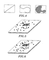
- FIGURE 5 shows the rectangular window corresponding to EXAMPLE QUERY 3 superimposed on the points shown in FIGURE 2 .
- Spatial Data Structures The problems which conventional database management methods have with spatial data have led to the development of a variety of special purpose data storage and retrieval methods called Spatial Data Structures.
- Many of the commonly used spatial data structures rely on the concept of tile based hierarchical trees.
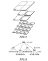
- FIGURE 7 shows a rectangular recursive decomposition of space while FIGURE 8 shows how the tiles formed by that decomposition can be organized to form a "tree" (a hierarchical data structure designed for searching). Data structures of this type are called Quad-Trees.
- FIGURE 9 shows the points from FIGURE 2 distributed into the "leaf-nodes" of this Quad-Tree.
- FIGURE 10 shows the subset of the Quad-Tree which is contacted by the Rectangular Window Retrieval of EXAMPLE QUERY 3 .
- All of the inspected points from the two nodes in FIGURE 10 are at least in the neighborhood of the rectangle, whereas some points inside the stripe in FIGURE 6 are literally at the far edge (bottom) of the coordinate system. While the difference in number of inspected points is not great due to the simplicity of this example, the performance contrast is dramatic when the number of point objects is very large.
- the Quad-Tree is much better suited to storing position based data because it simultaneously indexes along both axis of the coordinate system.
- each tile in the hierarchy corresponds to a "record" containing information which pertains to that tile. If the tile is at the root or at a branch level, the corresponding record will contain the coordinates of, and pointers to, the records for each child tile. If the tile is at the leaf level, the corresponding record contains the subset of the spatial data objects (point, line or polygon objects and their attributes) which are geometrically contained within the tile's perimeter.
- the Quad-Tree database "records" are stored in a disk file in breadth first or depth first order, with the root at the head of the file.
- Quad-Tree data structure exhibits O(log(N)) cost when the spatial density of data is fairly uniform, therefore resulting in a well balanced tree.
- the balance is driven by the construction algorithms which control the amount of branching.
- the amount of branching (and therefore the maximum depth) in a Quad-Tree is driven by an interaction between the local density of spatial data objects and the maximum number of such objects which can be accommodated in a leaf level record. Specifically, when the data storage in a leaf record fills up, the leaf is split into four children with its spatial data objects redistributed accordingly by geometric containment. Each time this happens, the local height of the tree increases by one. As a result of this algorithmic behavior, however, very high local data densities can cause Quad-Tree performance to degrade toward O(N) cost due to exaggerated tree depth.
- FIGURE 11 shows such a sequencing of a 4 ⁇ 4 tiling using the Peano-Hilbert curve.
- the resulting tiles are 50 units on a side.
- the tiles thus sequenced can be stored in records similar to the leaves in a Quad-Tree, where the data stored in each record corresponds to the subset contained within the tile's perimeter.
- the records can be simply indexed by a table which converts tile number to record location.
- the tiles can also be used as a simple computational framework for assigning tile membership.
- DATABASE TABLE 4 shows the business location database table enhanced with corresponding tile number field from FIGURE 11 .
- the tile number is determined by computing the binary representations of the X and Y column and row numbers of the tile containing the point, and then applying the well known Peano-Hilbert bit-interleaving algorithm to compute the tile number in the sequence. Building an index on the tile number field allows the records to be efficiently searched with geometric queries, even though they are stored in a conventional database. For instance, it is possible to compute the fact that the rectangular window SQL query shown in EXAMPLE QUERY 3 can be satisfied by inspecting only those records which are marked with tile numbers 8 or 9.
- the BusinessLocations database table enhance with a Tile field.
- the order function for this method is given by FORMULA 4 .
- the expected number of tiles is given by FORMULA 5 , (the 1 is added within each parentheses to account for the possibility of the window retrieval crossing at least one tile boundary).
- the value of A in FORMULA 4 is therefore an inverse geometric function of the granularity of the tiling which can be minimized by increasing the granularity of the tiling.
- the expected number of points per tile is given by FORMULA 6 .
- the value of B in FORMULA 4 is therefore roughly a quadratic function of the granularity of the tiling which can be minimized by decreasing the granularity of the tiling.
- the expected value of FORMULA 4 can therefore be minimized by adjusting the granularity of the tiling to find the point where the competing trends of A and B yield the best minimum behavior of the system.
- the expected number of records which will be sampled is a function of the average number of records in a tile multiplied by the average number of tiles needed to satisfy the query.
- the tile size By adjusting the tile size, it is possible to control the behavior of this method so that it retains the O(log(N)) characteristics of the database indexing scheme, unlike a simple index based only on X or Y coordinate.
- Oracle Corporation's implementation of two-dimensional "HHCODES" is an example of this type of scheme.
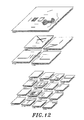
- FIGURE 12 shows how the linear and polygonal data objects from FIGURE 3 naturally fall into the various nodes of the example Quad-Tree. Note how many objects reside at higher levels of the Quad-Tree. Specifically, any object which crosses one of the lower level tiles boundaries must be retained at the next higher level in the tree, because that tile is the smallest tile which completely covers the object. This is the only way that the Quad-Tree tile hierarchy has of accommodating the object which might cross a boundary as a single entity.
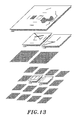
- FIGURE 13 shows the dramatic impact which the data that is moved up the hierarchical tree has on the example rectangular window retrieval. Since linear and polygonal data has size in addition to position, some substantial subset will always straddle the tile boundaries. As the number of objects in the database grows, the number of objects which reside in the upper nodes of the quad-tree will also grow, leading to a breakdown of the performance benefit of using the structure. This problem is shared by all hard tile-boundaried methods (Quad-Trees, K-D Trees, Grid-Cells and others).
- the R-Tree (or Range-Tree) is a data structure which has evolved specifically to accommodate the complexities of linear and polygonal data.
- R-Trees are a hierarchical search structure consisting of a root and multiple branch levels leading to leaves which contain the actual spatial data.
- R-Trees are built bottom-up to fit the irregularities of the spatial data objects.
- Leaf-level records are formed by collecting together data objects which have similar size and locality. For each record, a minimum bounding rectangle is computed which defines the minimum and maximum coordinate values for the set objects in the record.
- Leaf records which have similar size and locality are in turn collected into twig-level records which consist of a list of the minimum bounding rectangles of and pointers to each of the child records, and an additional minimum bounding rectangle encompassing the entire collection. These twig records are in turn collected together to form the next level of branches, iterating until the tree converges to a single root record.
- Well balanced R-Trees exhibit O(log(N)) efficiency.
- R-Trees The difficulty with R-Trees is that, since there definition is dependent on how the data content "fits" together to build the tree, the algorithms for building and maintaining R-Trees tend to be complicated and highly sensitive to that data content. Static applications of R-Trees, where the data content does not change, are the easiest to implement. Dynamic applications, where the data is constantly being modified, are much more difficult. This is in part because the edit operations which modify the geometric descriptions of the spatial data, by implication have the potential to change the minimum bounding rectangle of the containing record, which in turn can effect the minimum bounding rectangle of the parent twig record, and so on up to the root. Any operation therefore has the potential to cause significant reorganization of the tree structure, which must be kept well balanced to maintain O(log(N)) efficiency.
- the problem data object types are closed intervals of a single variable, for example, intervals of time.
- the problem data object types such as lines, circles and polygons are described by closed intervals of two variables.
- Three-dimensional spatial data which describe a three-dimensional surface has similar requirements for efficient organization.
- the added complexity is that three-dimensional spatial data consists of 3 independent variables (X, Y and Z) which have equal weight.
- three-dimensional geometric descriptions of lines, surfaces and volumes are also more complicated than two-dimensional lines and polygons, which make the data somewhat bulkier.
- databases of information can comprise hundreds of megabytes of data, thereby being very difficult to efficiently search.
- multidimensional data that is stored with the method and system of the present invention can be retrieved with far fewer processor cycles and disk seeks than in prior systems.
- each object within the spatial database would be assigned X and Y coordinates.
- Larger objects, such as lines, polygons and other shapes would be assigned a single location point within the coordinate system that would act like an anchor to hold the object to its position.
- a line might have a location point that corresponds to one of its ends, and the rest of the object would contain information about the other ends' X and Y coordinates, the line's thickness, color, or other features.
- each object within the spatial database would have a single location point, no matter how large the object was in the database.
- each location point could be assigned to a particular sub-region.
- These sub-regions are known as tiles because they resemble a series of tiles once superimposed over a coordinate system that included a set of spatial data. Each tile would, therefore, hold a particular set of spatial data.
- a user that knew which tiles held the desired information only needed to search those specific tiles.
- the system read those few tiles from memory and began the process of gathering objects from those tiles. This method thereby prevented the system from analyzing every object in the entire database for every computer user's request.
- the one embodiment reduces these previous problems by providing a series of overlaps between every tile in a spatial database.
- These overlapping tiles termed herein "shingles", represent tiles that overlap their nearest four neighbors.
- the area of overlap for any shingle can be pre-determined to provide the maximum efficiency.
- a spatial database holding map data might be programmed to have a shingle size of 10 square miles with each single overlap comprising 5 square miles.
- every shingle would have an overlap with its nearest four neighbors that is equal to the size of the neighboring shingles.
- the shingle overlap allows more data objects in the spatial database to be assigned to only one shingle and not split between multiple hard edged tiles. As discussed above, dividing an object across multiple tiles is very disadvantageous because it requires the system to track every tile that is assigned to a particular object.
- the purpose of the tiered shingle structure is to provide a logical framework for resolving Spatial Queries into the database in a timely and efficient manner.
- the spatial data structure is conceptual structure that provides the organization for indexing objects within a spatial data set.
- the tiered shingle structure does not have to be embodied in a specific computer data structure to be useful and effective.
- the Tiered Shingle Structure is part of a computational tool for organizing a set of spatial data objects, such as lines, squares and polygons into subsets based on their similar position and size in space.
- the tiered shingle structure can provide a mechanism for identifying those subsets of the database which contain the necessary and sufficient spatial data objects required by a specific spatial query into the database.
- the system and method of the present invention alleviates the problems found in prior systems of small objects which cross title boundaries being moved to higher levels in the tree.
- the layers of sub-regions are generated, the tiles are calculated to have areas which overlap. Therefore, no hard edges exist between tiles or an object might reside in two tiles simultaneously. These overlapping sub-regions are termed shingles. Because a shingle might overlap with, for example, one half of its closest neighbors, objects which fit into the large shingle region will remain at the lowest possible level.
- Another advantage of the present invention is that it improves the efficiency of individual databases because the shingle overlap size in each layer can be pre-programmed to provide the fastest access to the spatial database.
- the first level of shingling might have a shingle size of 5 square miles and divide the map database into 10,000 shingles.
- the second level of shingling might have a shingle size of 10 square miles and divide the map database into 2500 shingles. This will be discussed more specifically below in reference to Figure 12 .
- a method of organizing spatial data objects in a map database including referencing data objects as location points in a region to a coordinate system; separating the region into multiple sub-regions and assigning the data objects whose location point falls within a sub-region to the sub-region so long as no part of the object extends outside the sub-region by a predetermined amount.
- Also disclosed is a method of storing spatial data objects to a computer memory comprising the steps of (1) determining the size of each data object within a coordinate system; (2) assigning each spatial data object to a location point in the coordinate system; (3) calculating the boundaries of a first tier of overlapping sub-regions of the coordinate system so that each point in the coordinate system is assigned to at least one sub-region; (4) referencing each spatial data object that is smaller than the size of said sub-regions in the first tier to a specific sub-region of the coordinate system based on the location point of each spatial data object; and (5) storing the spatial data objects along with its reference to a specific sub-region to the computer memory.
- the present invention is a method and system for organizing large quantities of data.
- the examples used to illustrate the embodiment of this invention are for organizing map data, the techniques can be applied to other types of data.
- Other applicable data types include engineering and architectural drawings, animation and virtual reality databases, and databases of raster bit-maps.
- the purpose of the tiered shingle structure is to provide a logical framework for resolving spatial queries into a computer database in a timely and efficient manner.
- the tiered shingle structure does not have to be embodied in a specific computer data structure to be useful and effective.
- the tiered shingle structure is part of a computational tool for organizing a set of spatial data objects, such as lines, squares and polygons into subsets based on their similar position and size in space.
- the tiered shingle structure provides a mechanism for identifying those subsets of the database which contain the necessary and sufficient spatial data objects required by a specific spatial query into the database.
- the tiered shingle structure can run on an Intel ® processor based computer system in one preferred embodiment. However, other computer systems, such as those sold by Apple ® , DEC ® or IBM ® are also anticipated to function within the present invention.
- FIGURE 14 is an illustration of a three level tiered shingle structure as it would be applied to the example coordinate plane shown in Figure 1 .
- This Tiered Shingle Structure is similar to the regular quadrant-based decomposition of the coordinate plane shown in FIGURE 7 .
- each level consists of overlapping shingles. The overlap between adjacent shingles will be discussed in more detail below, but is indicated by the shaded bands 22 in FIGURE 14 .
- shingles 1-18 formed by regular overlapping squares or rectangles which are normal to the coordinate axis are the easiest to understand and implement, though other configurations are possible.
- the finest level in a Tiered Shingle Structure (shingles 1-16 in FIGURE 14 ) is designed to serve as the indexing medium for the vast majority of the spatial data.
- the spatial objects which extend beyond the edge of the central portion of the shingle by more than a predetermined amount (e.g., its overlap will be assigned to the next higher tier in the hierarchy).
- the granularity (size of shingle and amount of overlap) of that finest level can be tuned to balance between the competing trends of maximizing the number of spatial data objects which "fit" in that level of shingling (accomplished by increasing the size of the shingles), versus maximizing the degree of partitioning (accomplished by decreasing the size of the shingles).
- the coarser levels of shingles (a single level in FIGURE 14 consisting of shingles 17-20) serve as an alternative indexing medium for those objects which do not fit in the finest level (i.e., any object which is spatially too large to fit within a particular tile), including its shingled overlap with its nearest neighbors. Note that the absolute size of the overlap increases as the tile size increases in each successively coarser level.
- the top-level shingle 21 FIGURE 14
- FIGURE 15 is an illustration of how each of the linear and polygonal objects depicted in the FIGURE 3 are organized within the Tiered Shingle Structure data structure of the present invention.
- each shingle contains a subset of the objects having a similar position and size.
- the benefit of regular overlapping tiles provided by the data structure of the present invention can be seen by comparing the present invention data structure organization of FIGURE 15 with the data structure organization of FIGURE 12 .
- This shingled overlap system allows the small data objects which were located on the arbitrary tile boundaries of the prior art data structures (the bulk of the population in tiles 100, 110, 120, 130 and 140 in FIGURE 12 ) to remain within the lowest level in the Tiered Shingle Structure.
- any object which is smaller than the size of the overlap at any given level is guaranteed to fit into some shingle at or below that level.
- many objects which are larger than the shingle overlap may also fit within a lower level.
- shingles 1, 6 and 9 in FIGURE 15 are mostly populated by such objects. Note the position of those same objects in FIGURE 12 .
- DATA TABLE 2 provides a numerical comparison of the data object partitioning in FIGURE 15 versus FIGURE 12 .
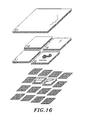
- FIGURE 16 to FIGURE 13 shows why the improved partitioning scheme provided by the Tiered Shingle Structure translates into improved rectangular window query performance over an equivalent structure based on prior art. While the number of tiles which need to be inspected during a data query has slightly increased from five in FIGURE 13 to seven in FIGURE 16 , the number of data objects which must be inspected has dropped by nearly half (sixteen versus thirty-one). This drop is directly due to the fact that many more objects can be fit into the finer partition levels with only a slight increase in the size of each partition. As discussed above, a spatial data query must inspect every object within each tile that meets the parameters of the query.
- each of the data objects within the top-level tile 100 must be inspected to determine whether it meets the parameters of the spatial data query. Because so many more data objects are able to reside in the smaller tile structures when organized by the method of the present invention, there are many fewer data objects to inspect during a spatial data query. For this reason, computer databases that are organized by the system of the present invention can be searched more rapidly than prior art systems.
- Shingle Assignment Functions convert the spatial description of a spatial data object into a "Shingle-Key".
- a Shingle-Key is a number which uniquely represents a specific shingle in a Tiered Shingle Structure.
- Query Control Functions convert the query specification of certain common geometric queries into a list of the necessary and sufficient Shingle-Keys which "contain" the data needed to satisfy the query.
- Appendix A contains a code written in the C programming language for implementing.
- the KeyForBox and KeyRectCreate function calls both expect their corresponding spatial description parameters to be expressed in Longitude (X1 and X2) and Latitude (Y1 and Y2) coordinates with decimal fractions.
- nLevelMask which controls which levels are to be included in the Tiered Shingle Structure
- nLevelLap which controls the amount of overlap between adjacent shingles.
- Shingle-Keys generated by a Shingle Assignment Function are used to partition the members of a set of spatial data into subsets where all members of a subset have the same Shingle-Key. This means that each member of a subset can be "fit” onto the same shingle (eg: the size of the minimum bounding box that contains the object is not larger than the tile). This further means that all members of a subset have a similar spatial size and position. Indexing and clustering the data in the storage mechanism (common database management practices intended to improve efficiency) by Shingle-Key are therefore very effective, since spatial queries usually select objects which, as a group, have similar position and size.
- PROCEDURE TABLE 1 shows a set of computational steps that will derive the Shingle-Key corresponding to a particular spatial data object.
- the steps in this table correspond to lines 0536 through 0652 of the KeyForBox function in Appendix A. The details of some of these steps are expanded upon in subsequent paragraphs.
- Step 1 Compute the Minimum Bounding Rectangle (MBR) of the Spatial Description.
- Step 2 Repeat Steps 3-6 for each sequential level in the structure, starting with the finest: Step 3 At the current level, determine which Shingle's minimum corner is "closest-to" but also "less-then-or-equal-to" the minimum corner of the MBR.
- Step 4 Determine the maximum corner of this Shingle.
- Step 5 It the maximum corner of this Shingle is "greater-than" the maximum corner of the MBR, then have found the smallest containing shingle. Goto Step 7.
- Step 6 couldn't find smaller shingle, therefore assign object to the top-level shingle.
- Step 7 Determine the Shingle-Key for the current Shingle.
- Step 1 given in PROCEDURE TABLE 1 is computing the Minimum Bounding Rectangle of the Spatial Data Object.
- the Minimum Bounding Rectangle of a spatial data object is the smallest rectangle which is normal to the coordinate axes and completely contains the object.
- the typical method of representing a Minimum Bounding Rectangle is with two points: the minimum point (lower-left corner in conventional coordinate systems) and the maximum point (upper-right corner).
- FIGURE 4 illustrates the minimum bounding rectangles of a few common types of spatial objects.
- PROCEDURE TABLE 2 describes how minimum bounding rectangles can be computed for a variety of common types of spatial data objects. In some cases, a slight over-estimate of the Minimum Bounding Rectangle may be used when the precise computation is too expensive.
- Minimum Bounding Rectangles can be derived for some common types of Spatial Data Objects.
- Point The minimum and maximum points are the same as the Point itself. Segment The minimum point consists of the lesser x-coordinate and lesser y-coordinate of the two end points; the maximum point consists of the greater x-coordinate and greater y-coordinate of the two end points.
- Polyline The minimum point consists of the least x-coordinate and least y-coordinate found in the list of points for the Polyline; the maximum point consists of the greatest x-coordinate and greatest y-coordinate found in the list of points for the Polyline.
- the minimum point consists of the least x-coordinate and least y-coordinate found in the list of points for the Polygon; the maximum point consists of the greatest x-coordinate and greatest y-coordinate found in the list of points for the Polygon.
- Circle The minimum point is found by subtracting the radius of the Circle from each coordinate of the center of the Circle; the maximum point is found by adding the radius of the Circle to each coordinate of the center of the Circle B-Spline
- the minimum point can be estimated by selecting the least x-coordinate and least y-coordinate found in the set of four point used to construct the B-Spline; the maximum point can be estimated by selecting the greatest x-coordinate and greatest y-coordinate found in the set of four point used to construct the B-Spline.
- a B-spline is constructed from two end-points and two control-points.
- Step 3 of PROCEDURE TABLE 1 a determination is made whether the Shingle in the current level who's minimum point (lower-right corner) is both closest-to and less-than-or-equal-to the Minimum Bounding Rectangle of the spatial object. If the Tiered Shingle Structure is based on a regular rectangular or square tiling of the coordinate plane (as illustrated in FIGURE 14 and described in Appendix A ) then the candidate shingle is the one corresponding to the tile which contains the minimum point of the Minimum Bounding Rectangle. In the KeyForBox function of Appendix A, lines 0590 and 0591, the coordinates of the minimum point of the Shingle are computed directly using binary modular arithmetic (the tile containment is implied).
- Step 4 of PROCEDURE TABLE 1 the maximum point (upper right corner) of the candidate shingle is calculated. That point can be determined directly from the minimum point of the shingle by adding the standard shingle width for the current level to the x-coordinate and adding the standard shingle height for the current level to the y-coordinate. In Appendix A , this calculation is performed in lines 0598 through 0601 of the KeyForBox function. Since the Tiered Shingle Structure used in Appendix A is based on overlapping squares, the same value is added to each coordinate.
- Step 5 of PROCEDURE TABLE 1 the maximum corner of the shingle is compared to the maximum corner of the Minimum Bounding Rectangle ( MBR ). This is accomplished through a piece-wise comparison of the maximum x-coordinate of the shingle to the maximum x-coordinate of the MBR and the maximum y-coordinate of the shingle to the maximum y-coordinate of the MBR . If each coordinate value of the shingle is greater than the corresponding value for the MBR , then the maximum corner of the shingle is said to be greater than the maximum corner of the MBR . In Appendix A , this calculation is performed on lines 0609 and 0610 of the KeyForBox function.
- Step 6 of PROCEDURE TABLE 1 is performed if, and only if, the repeat loop of Steps 2-5 is exhausted without finding a shingle which fits the Minimum Bounding Rectangle.
- the spatial object which is represented by the Minimum Bounding Rectangle therefore does not fit within any of the lower levels (eg: tiers) of the shingle structure. It therefore by definition must fit within the top-level shingle.
- this step is performed on lines 0651 and 0652 of the KeyForBox function.
- Step 7 given in PROCEDURE TABLE 1 determines the Shingle-Key for the shingle which was found to "best-fit" the data object.
- the Peano-Hilbert space filling curve is used to assign Shingle-Key numbers via the KeyGenerator function call shown in lines 0623-0625 of the KeyForBox function.
- the KeyGenerator function is implemented in lines 0043-0485 of Appendix A .
- the parameters given to the KeyGenerator function include the coordinates of the minimum point of the Shingle, and the corresponding level in the Tiered Shingle Structure. Note that the uniqueness of Shingle-Key numbers across different levels is guaranteed by the statement on line 0482 of Appendix A .
- the second class of functions are used for controlling spatial queries into the computer database. Functions of this class convert the query specification for certain common geometric queries into a list of the necessary and sufficient shingle keys which contain the data needed to satisfy the query.
- the list of shingle-keys may be expressed either as an exhaustive list of each individual key, or as a list of key ranges (implying that all keys between and including the minimum and the maximum values of the range are needed).
- Step 1 Identify the set of shingles which overlap the region being queried
- Step 2 Repeat Steps 3-5 for each identified shingle
- Step 3 retrieve from the computer database the subset of spatial data which has been assigned the identified shingle-keys
- Step 4 Repeat Step 5 for each object in the subset Step 5 Test the object for overlap with the region being queried; Retain each object which passes the test
- the set of shingles which overlap the queried region is the union of the shingles from each hierarchical level which overlap the region.
- the shingles for a given level can be found by first identifying all the shingles which touch the perimeter of the region, and then filling in with any shingles missing from the middle section.
- One method of finding all the shingles which touch the perimeter of the query is to computationally trace the path of each component through the arrangement of shingles, taking care to eliminate redundant occurrences.
- a method of filling in the shingles missing from the middle section is to computationally scan bottom-to-top and left-to-right between the Shingles found on the perimeter.
- the software program in Appendix A implements one Query Control Function Set in lines 0655-1135. This set of functions identifies all shingles which overlap the given Longitude/Latitude rectangle. PROCEDURE TABLE 4 shows the algorithmic usage of this function set.
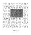
- FIGURE 17 illustrates how the Peano-Hilbert space-filling curve winds its way contiguously through each tile in one level of a spatial database.
- Step 1 Create a KeyRect structure for the rectangle using KeyRectCreate
- Step 2 For each Shingle-Key range (MinKey, MaxKey) returned by KeyRectRange, repeat steps 3-5
- Step 3 Select all Objects where ObjectKey ⁇ MinKey and ObjectKey ⁇ MaxKey
- Step 4 For each selected Object, repeat step 5
- Step 5 If ObjectSpatialData is overlaps the rectangle, process the Object
- Step 6 Destroy the KeyRect structure using KeyRectDestroy
- a general polygonal retrieval is similar to a rectangular window retrieval in that the purpose of the query is to fetch all database objects which are inside or which touch the boundary of an arbitrary polygon.
- SQL System Query Language
- DATABASE TABLE 5 illustrates a sample database table containing data objects representing a portion of the street segments from FIGURE 3 .
- the Shingle column contains the assigned Shingle-Keys from FIGURE 15 .
- the X1/Y1 and X2/Y2 columns contain the coordinates of the minimum bounding rectangle for each object within the chosen shingle.
- EXAMPLE QUERY 4 shows how DATABASE TABLE 5 can be queried to find a portion of each data object with a minimum bounding rectangle that overlaps a the rectangular query window, assuming a functional interface similar to Appendix A existed for this tiered shingle structure.
- This query corresponds to Steps 3-5 in PROCEDURE TABLE 4 . As such, this query would have to be repeated once for each key range in order to find all segments which overlap the rectangle.
- the key ranges which correspond to EXAMPLE QUERY 4 window are 8-9, 17-20 and 21-21. Note how running this query using these key ranges on DATABASE TABLE 5 will result in selecting the single overlapping segment assigned to Shingle 9. Other objects from FIGURE 3 not listed in DATABASE TABLE 5 also overlap the window.
- Step 5 Create index on Shingle Field. Implement clustering, if possible Record Insert Step 1 Prior to Insert: Compute Shingle-Key using KeyForBox on the Minimum Bounding Rectangle of the Spatial Data.
- Step 2 Insert record into database, including Shingle-Key.
- Step 2 If new Shingle-Key is different then old Shingle-Key, include the new Shingle-Key in the update. Record Delete For each selected Object, repeat step 5.
- Database Unload Destroy the KeyRect structure using KeyRectDestroy.
- the improved partitioning identified in the earlier comparison of FIGURES 12 and 15 can be validated by measuring how the present invention behaves when given a large quantity of real map data.
- DATA TABLE 3 shows the results of one such measurement.
- the data used to perform these measurements is an extract of street segments from a U.S. Census Bureau Topographically Integrated Geographic Encoding and Referencing (TIGER) database file of Los Angeles County, CA. Census TIGER files comprise the defacto industry standard street map data source. Los Angeles County is a good representative choice because of its large size (426367 segments in this extract) and diverse coverage (dense urbanized core, sprawling suburbia and sparsely populated mountain and desert regions).
- the Lev column indicates the level of the tile/shingle structure, 0 being the finest partitioning, 14 being the most coarse, 15 being the top-level compartment.
- the Segs column accumulates the total number of TIGER street segments which naturally fit at this level (i.e., do not cross tile/shingle boundaries - returned through the pnLevel parameter of the KeyForBox function).
- the Shing and Tiles columns accumulate the total number of unique Key values returned by the KeyForBox function.
- the Av column computes the average number of segments per unique tile/shingle.
- the Mx column shows the maximum number of segments which were associated with any one tile/shingle.
- the Shingles-with-25%-Overlap columns in DATA TABLE 3 shows how efficiently the tiered shingle structure organizes this set of data. Note the shallow distribution of segments into the lower levels of the structure: over 95 % of the segments have settled into the lowest level of the data structure. Note how few additional levels are needed, and also the low average and maximum number of segments per shingle in those levels.
- FORMULA 7 is derived from FORMULA 4 which established the behavior of a tile-based method for storing points in a database table.
- the primary refinement in FORMULA 7 is that a sum must be accumulated to account for the spread of objects across multiple levels.
- FORMULA 11 is derived from FORMULA 5 , primarily by changing the offset factor from 1 to 2 to account for the fact that the overlap will tend to increase the number of tiles touched by the query window.
- TABLE 13 shows the plug-in values for A L and B L for a 0.016° Longitude ⁇ 0.0145° Latitude rectangular window (a roughly 1 mile square at Los Angeles, CA's Latitude).
- FORMULA 7 represents a worst case which can be greatly improved in practice.
- the value of A L in the portion of the formula A L ⁇ log(N) can substantially be reduced by using the Peano-Hilbert space filling curve to sequence the shingles as they are stored in the computer database, as is done in the software implementation given in Appendix A.
- Use of that curve guarantees that many adjacent shingles will be numbered consecutively. For instance, in any arbitrary 3x3 grouping of adjacent shingles in a field sequenced with the Peano-Hilbert curve, there can be at most 4 consecutive sequences (refer to FIGURES 8 and 17 ).
- TABLE 13 Computed values for A L for an arbitrary 1 square mile rectangular window around Los Angeles County, CA. Measure values for B L mile from TABLE 7 .
- the present invention provides an efficient method and system for organizing large quantities of data.
- databases of information can comprise hundreds of megabytes of data, thereby being very difficult to efficiently search.
- multidimensional data that is stored with the method and system of the present invention can be retrieved with far fewer processor cycles and disk seeks than in prior systems.
- each spatial object is assigned to a particular sub-region.
- These sub-regions are known as tiles because they resemble a series of tiles once superimposed over a set of spatial data. Each tile would, therefore, hold a particular set of spatial data.
- a user that knew which tiles held the desired information only needed to search those specific tiles.
- the system can read those few tiles from memory and begin the process of gathering objects from those tiles. This method thereby prevents the system from analyzing every object in the entire database for every computer user's request.
- the present invention provides a series of overlaps between every tile in a spatial database.
- These overlapping tiles termed herein "shingles", represent tiles that overlap their nearest neighbors.
- the area of overlap for any shingle is pre-determined to provide the maximum efficiency.
- the shingle overlap allows more data objects in the spatial database to be assigned to only one shingle and not split between multiple hard edged tiles, as was done in prior systems. As discussed above, dividing an object across multiple tiles is very disadvantageous because it requires the system to track every tile that is assigned to a particular object.
- the system and method of the present invention alleviates the problem of small objects which cross title boundaries being moved to higher levels.
- the layers of sub-regions are generated, they are calculated to have areas of overlap.
- the present invention improves the efficiency of individual databases because the shingle overlap size in each layer can be programmed to provide the fastest access to the spatial database.
Landscapes
- Engineering & Computer Science (AREA)
- Theoretical Computer Science (AREA)
- Databases & Information Systems (AREA)
- Data Mining & Analysis (AREA)
- Physics & Mathematics (AREA)
- General Engineering & Computer Science (AREA)
- General Physics & Mathematics (AREA)
- Remote Sensing (AREA)
- Software Systems (AREA)
- Information Retrieval, Db Structures And Fs Structures Therefor (AREA)
- Processing Or Creating Images (AREA)
Description
- This invention relates to computer databases. Specifically, this invention relates to methods of indexing database records which contain information describing the position, size and shape of objects in two and three-dimensional space.
- The purpose of a data structure is to organize large volumes of information, allowing the computer to selectively process the data structure's content. The motivation for this is simple: you always have more data than your time requirements, processor speed, main memory and disk access time allow you to process all at once. Depending on the nature of the data and application, data organizing strategies may include partitioning the content into subsets with similar properties or sequencing the data to support indexing and hashing for fast random access. Databases and database management systems extend these concepts to provide persistent storage and transaction controlled editing of the structured data.
- Spatial data such as that describing a two-dimensional map is no different in its need for efficient organization. Map data is particularly demanding in this regard. A comprehensive street map for a moderate sized community may consist of tens to hundreds of thousands of individual street segments. Wide area maps of LA or New York may contain millions of segments. The content of each map data object can also be some what bulky. For example, a record for an individual street segment may include the coordinates of its end points, a usage classification, the street name, street address ranges, left and right side incorporated city name and postal codes.
- However, spatial data at its core poses a particularly vexing organizational problem because it tries to organize objects within two-dimensional space. Spatial coordinates consist of two (or more) values which are independent, but equally important for most spatial queries. Established data structures and database methods are designed to efficiently handle a single value, and not representations of multi-dimensional space.
- This difficulty can be illustrated by considering the problem of creating an application which presents a small window of map data (for instance, the square mile surrounding a house) from a database of a few hundred thousand spatial objects (a map of the city surrounding the house). The motivation for doing this is really two fold: first, the typical resolution of a computer monitor is limited, allowing only a certain amount information to be expressed. Secondly, even if all the data fit within the monitor, the data processing time to calculate this much information (fetching, transforming, clipping, drawing) would be far too long for the average personal computer.
- To solve this problem, it is advantageous to find all of the street segments which appear in the "window" that will be generated on the monitor, and avoid as many as possible which do not. Thus, all objects which are within a particular range of x-coordinate (or longitude) values and y-coordinate (or latitude) values will be gathered. This problem is generally known as rectangular window retrieval, and is one of the more fundamental types of spatial queries. This method will be used in the following sections as a method for gauging the effectiveness of each of the following organizational methods.
- The most heavily researched and commonly used spatial data structures (data structures used to organize geographic and geometric data) rely on the concept of tile-based hierarchical trees. A tile in this context is a rectangular (or other regularly or irregularly shaped) partitioning of coordinate space, wherein each partition has a distinct line separating one tile from another so that no single point in the coordinate system lies within more than one tile. A hierarchical tree is one structure for dividing coordinate space by recursively decomposing the space into smaller and smaller tiles, starting at a root that represents the entire coordinate space. In this system, a "hard edge" between tiles means that every point in the space resides exactly one tile at each level of the hierarchy. No point can coexist in more than one tile.
- One example of a well-known hierarchical tree is the quad-tree data structure. In one example, the quad-tree could represent the surface of the Earth. At the root of the quad-tree is a node representing the entire surface of the Earth. The root, in turn, will have four children representing each quadrant of Latitude and Longitude space: east of Greenwich and north of the Equator, east of Greenwich and south of the Equator, west of Greenwich and north of the Equator and finally, west of Greenwich and south of the equator. Points on Greenwich and the Equator are arbitrarily defined to be in one quadrant or the other. Each of these children are further subdivided into more quadrants, and the children of those children, and so on, down to the degree of partitioning which is required to support the volume and density of data which is to be stored in the quad-tree.
- The principle problem with quad-tree structures is that they are unbalanced. Because each node in the tree has a limited data storage capacity, when that limit is exceeded, the node must be split into four children, and the data content pushed into lower recesses of the tree. As a result, the depth of a quad-tree is shallow where the data density is low, and deep where the data density is high. For example, a quad-tree used to find population centers on the surface of the Earth will be very shallow (e.g., have few nodes) in mid-ocean and polar regions, and very deep (e.g., have many nodes) in regions such as the east and south of the United States.
- Since quad-trees are inherently unbalanced, the rectangular window retrieval behavior of a quad-tree is difficult to predict. It is difficult for software to predict how many nodes deep it may have to go to find the necessary data. In a large spatial database, each step down the quad-tree hierarchy into another node normally requires a time-consuming disk seek. In addition, more than one branch of the tree will likely have to be followed to find all the necessary data. Second, when the content of the data structure is dynamic, efficient space management is problematic since each node has both a fixed amount of space and a fixed regional coverage. In real world data schemes, these two rarely correspond. There are several variations on the quad-tree which attempt to minimize these problems. However, inefficiencies still persist.
- So far, data structures containing points have only been discussed where each spatial object comprises a single set of coordinates. Lines, curves, circles, and polygons present a further complexity because they have dimensions. Therefore, these objects no longer fit neatly into tile based data structures, unless the tiling scheme is extremely contrived. There will always be some fraction of the objects which cross the hard edged tile boundaries from one coordinate region to another. Note that this fact is true regardless of the simplicity of an object's description. For example, a line segment described by its two end points, or a circle described by its center point and radius.
- A simple, and commonly used way around this problem is to divide objects which cross the tile boundaries into multiple objects. Thus, a line segment which has its end points in two adjacent tiles will be split into two line segments; a line segment which starts in one tile, and passes through fifty tiles on its way to its other end will be broken into fifty-two line segments: one for each tile it touches.
- This approach can be an effective strategy for certain applications which are read-only. However, it is a poor strategy for data structures with dynamic content. Adding new data objects is relatively simple, but deleting and modifying data are more difficult. Problems arise because the original objects are not guaranteed to be intact. If a line segment needs to be moved or removed, it must somehow be reconstituted so that the database behaves as expected. This requires additional database bookkeeping, more complicated algorithms and the accompanying degradation in design simplicity and performance.
- Another general problem related to organizing multidimensional objects is that many of these objects are difficult to mathematically describe once broken up. For example, there are numerous ways in which a circle can overlap four adjacent rectangular tiles. Depending on placement, the same sized circle can become two, three or four odd shaped pieces. As with a heavily fragmented line segment, the original "natural" character of the object is effectively lost.
- An alternate strategy is to use indirection, where objects which cross tile boundaries are multiply referenced. However, each reference requires an extra step to recover the object, and the same object may be retrieved more than once by the same query, requiring additional complexity to resolve. When the number of objects in the database becomes large, this extra level of indirection becomes too expensive to create a viable system.
- Another strategy used with quad-trees is to push objects which cross tile boundaries into higher and higher levels of the tree until they finally fit. The difficulty with this strategy is that when the number of map objects contained in the higher nodes increases, database operations will have to examine every object at the higher nodes before they can direct the search to the smaller nodes which are more likely to contain useful information. This results in a tremendous lag time for finding data.
- Abel D J et al: "A data structure and query algorithm for a database of areal entities", Australian Computer Journal Australia, vol. 16, no. 4, February 1984 (1984-02), pages 147-154, XP008044407, ISSN: 0004-8917 relates to the technology of the invention. In this document, an entity is addressed by a limited number of sub quadrants which cover it, and an algorithm for the rectangle retrieval problem is presented.
- In Samet H: "The quadtree and related hierarchical data structures", Computing Surveys USA, vol. 16, no. 2, June 1984 (1984-06), pages 187-260, XP002321669, ISSN: 0360-0300 a tutorial survey is presented of the quadtree and related hierarchical data structures. The emphasis is on the representation of data used in applications in image processing, computer graphics, geographic information systems, and robotics.
- In Samet H: "A quadtree medial axis transform" Communications of the ACM USA, vol. 26, no. 9, September 1983 (1983-09), pages 680-693, XP002321670, ISSN: 0001-0782, a number of methods of representing images are presented, among which are borders, arrays, and skeletons. A discussion is also given on the quadtree approach to image representation.
- As discussed above, data which describes the position, size and shape of objects in space is generally called spatial data. A collection of spatial data is called a Spatial Database. Examples of different types of Spatial Databases include maps (street-maps, topographic maps, land-use maps, etc.), two-dimensional and threedimensional architectural drawings and integrated circuit designs.
- Conventional Database Management Systems (DBMS) use indexing methods to optimize the retrieval of records which have specific data values in a given field. For each record in the database, the values of the field of interest are stored as keys in a tree or similar indexing data structure along with pointers back to the records which contain the corresponding values.
- DATABASE TABLE 1 shows an example of a simple database table which contains information about former employees of a fictional corporation. Each row in the table corresponds to a single record. Each record contains information about a single former employee. The columns in the table correspond to fields in each record which store various facts about each former employee, including their name and starting and ending dates of employment.
-
The FormerEmployee database table. Name StartDate EndDate Other ... P. S. Buck 6/15/92 8/2/95 Willy Cather 1/27/93 6/30/93 Em Dickinson 9/12/92 11/15/92 Bill Faukner 7/17/94 2/12/95 Ernie Hemmingway 6/30/91 5/14/93 H. James 10/16/91 12/4/92 Jim Joyce 11/23/92 5/8/93 E. A. Poe 1/14/93 4/24/95 -
EXAMPLE QUERY 1 shows a SQL query which finds the names of all former employees who started working during 1993. If the number of records in the former employee database were large, and the query needs to be performed on a regular or timely basis, then it might be useful to create an index on the StartDate field to make this query perform more efficiently. Use of a sequential indexing data structure such as a B-tree effectively reorders the database table by the field being indexed, as is shown in DATABASE TABLE 2. The important property of such sequential indexing methods is that they allow very efficient search both for records which contain a specific value in the indexed field and for records which have a range of values in the indexed field. - SQL to find all former employees hired during 1993.
select Name from FormerEmployee where StartDate ≥ 1/1/93 and StartDate ≤ 12/31/93 -
The FormerEmployee table indexed by StartDate. Name StartDate EndDate Other ... Ernie Hemmingway 6/30/91 5/14/93 H. James 10/16/91 12/4/92 P. S. Buck 6/15/92 8/2/95 Em Dickinson 9/12/92 11/15/92 Jim Joyce 10/23/92 5/8/93 E. A. Poe 1/14/93 4/24/95 Willy Cather 1/27/93 6/30/93 Bill Faukner 7/17/94 2/12/95 - For analytical purposes, the efficiencies of computer algorithms and their supporting data structures are expressed in terms of Order functions which describe the approximate behavior of the algorithm as a function of the total number of objects involved. The notational short hand which is used to express Order is O(). For data processing algorithms, the Order function is based on the number of objects being processed.
- For example, the best sorting algorithms are typically performed at a O( N x log(N) ) cost, where N is the number of records being sorted. For data structures used to manage objects (for instance, an index in a database), the Order function is based on the number of objects being managed. For example, the best database indexing methods typically have a O( log(N) ) search cost, where N is the number of records being stored in the database. Certain algorithms also have distinct, usually rare worst case costs which may be indicated by a different Order function. Constant functions which are independent of the total number of objects are indicated by the function O( K ).
- B-trees and similar Indexed Sequential Access Methods (or ISAMs) generally provide random access to any given key value in terms of a O(log(N)) cost, where N is the number of records in the table, and provide sequential access to subsequent records in a O(K) average cost, where K is a small constant representing the penalty of reading records through the index, (various strategies may be employed to minimize K, including index clustering and caching). The total cost of performing
EXAMPLE QUERY 1 is therefore O( log(N) +( M × K )), where M is the number of records which satisfy the query. If N is large and M is small relative to N, then the cost of using the index to perform the query will be substantially smaller than the O(N) cost of scanning the entire table. DATA TABLE 1 illustrates this fact by showing the computed values of some Order functions for various values of N and M. This example, though quite simple, is representative of the widely used and generally accepted database management practice of optimizing queries using indexes. - Cost of retrieving consecutive records from a database table via an index.
O(log(N) +( M × K )) where N = number of records in the table, M = number of consecutive records which satisfy the query, K = constant extra cost of reading records through the index. -
EXAMPLE QUERY 2 shows a SQL query which finds the names of all former employees who worked during 1993. UnlikeEXAMPLE QUERY 1, it is not possible to build an index using traditional methods alone which significantly improvesEXAMPLE QUERY 2 for arbitrary condition boundaries, in this case, an arbitrary span of time. From a database theory point of view, the difficulty with this query is due to the interaction of the following two facts: because the two conditions are on separate field values, all records which satisfy one of the two conditions need to be inspected to see if they also satisfy the other; because each condition is an inequality, the set of records which must be inspected therefore includes all records which come either before or after one of the test values (depending on which field value is inspected first). - SQL to find all former employees who worked during 1993.
select Name from FormerEmployee where EndDate ≥ 1/1/93 and StartDate ≤ 12/31/93 - Consider the process of
satisfying EXAMPLE QUERY 2 using the index represented by DATABASE TABLE 2. The cost of performingEXAMPLE QUERY 2 using an index based on either of the two fields would be O(K×N/2) average cost and O(K×N) worst-case cost. In other words, the query will have to look at half the table on average, and may need to inspect the whole table in order to find all of the records which satisfy the first of the two conditions. Since the cost of scanning the entire table without the index is O(N), the value of using the index is effectively lost (refer to TABLE 3). Indeed, when this type of circumstance is detected, query optimizers (preprocessing functions which determine the actual sequence of steps which will be performed to satisfy a query) typically abandon the use of an index in favor of scanning the whole table. - Cost of retrieving all records which overlap an interval using a conventional database index on the start or end value.
O(K×N/2) average, O(K×N) worst case. -
Comparison of Order function results for various values of N and M. A K value of 1.5 is used for the purpose of this example. N, O(N) M O(log(N)) O(log(N)+(M×K)) I O(K × N / 2) 100 5 2 10 75 100 10 2 17 75 100 50 2 77 75 1000 5 3 11 750 1000 10 3 18 750 1000 50 3 78 750 10000 5 4 12 7500 10000 10 4 19 7500 10000 50 4 79 7500 - From a more abstract point-of-view, the difficulty with this example is that there is actually more information which the conventional database representation does not take into account. StartDate and EndDate are in fact two different facets of a single data item which is the contained span of time. Put in spatial terms, the StartDate and EndDate fields define two positions on a Time-Line, with size defined by the difference between those positions. For even simple one-dimensional data, conventional database management is unable to optimize queries based on both position and size.
- Spatial databases have a particularly demanding need for efficient database management due to the huge number of objects involved. A comprehensive street map for a moderate sized community may consist of tens to hundreds of thousands of individual street blocks; wide area maps of Los Angeles, CA or New York, NY may contain more than a million street blocks. Similarly, the designs for modem integrated circuits also contain millions of components.
-
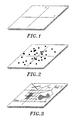
FIGURE 1 illustrates a coordinate plane with X- and Y-axes. For the purpose of the following example, the size of the plane is chosen to be 200×200 coordinate units, with the minimum and maximum coordinates values of -100 and 100 respectively for both X and Y. However, it should be noted that the principles discussed for the following example can be applied to any bounded two-dimensional coordinate system of any size, including, but not limited to planer, cylindrical surface and spherical surface coordinate systems. The latitude/longitude coordinate system for the earth's surface, with minimum and maximum latitude values of -90 degrees and +90 degrees, and minimum and maximum longitude values of -180 degrees and + 180 degrees, is an example of one such spherical coordinate system. -
FIGURE 2 illustrates a distribution of points on theFIGURE 1 plane. Ad discussed above, points are the simplest type of spatial data object. Their spatial description consists of coordinate position information only. An example of non-spatial description commonly associated with point objects might include the name and type of a business at that location, e.g., "Leon's BBQ", or "restaurant". -
FIGURE 3 illustrates a distribution of linear and polygonal spatial data objects representing a map (note that the text strings "Hwy 1" and "Hwy 2" are not themselves spatial data objects, but rather labels placed in close proximity to their corresponding objects). The spatial descriptions of linear and polygonal data objects are more complex because they include size and shape information in addition to solely their position in the coordinate system. An example of non-spatial description commonly associated with linear map objects might include the names and address ranges of the streets which the lines represent, e.g., "100-199 Main Street". An example non-spatial description commonly associated with polygonal map objects are the name and type of the polygon object, e.g., "Lake Michigan", "a great lake". -
FIGURE 4 illustrates the Minimum Bounding Rectangles (MBRs) of various of linear and polygonal spatial data objects. The Minimum Bounding Rectangle of a spatial data object is the smallest rectangle orthogonal to the coordinate axis which completely contains the object. Minimum Bounding Rectangles are typically very easy to compute by simple inspection for the minimum and maximum coordinate values appearing in the spatial description. In spatial data storage and retrieval methods, Minimum Bounding Rectangles are often used represent the approximate position and size of objects because the simple content (two pairs of coordinates) lends itself to very efficient processing. - DATABASE TABLE 3 shows how some of the points from
FIGURE 2 might be represented in a regular database table. The points in DATABASE TABLE 3 correspond to the subset of the points shown inFIGURE 2 indicated by the * markers.EXAMPLE QUERY 3 shows a SQL query which fetches all points within a rectangular window. A rectangular window query is among the simplest of the commonly used geometric query types. Inspection reveals that "Emily's Bookstore" is the only record from DATABASE TABLE 3 which will be selected by this query.FIGURE 5 shows the rectangular window corresponding toEXAMPLE QUERY 3 superimposed on the points shown inFIGURE 2 . -
A conventional database table containing some business locations. X Y Name Type -42 25 Leon's BBQ Restaurant 9 -34 Super Saver Grocery Store 17 21 Emily's Books Book Store 68 -19 Super Sleeper Motel -84 7 Bill's Garage Gas Station - SQL to find all businesses in a window.
select Name, Type from BusinessLocation where X ≥ 10 and X ≤ 35 and Y ≥ 15 and Y ≤ 40 - The principle problem illustrated by this example is that the traditional query optimization method of building a simple index doesn't work well enough to be useful. Consider building an index based on the X field value. Use of this index to satisfy
EXAMPLE QUERY 3 will result in an over-sampling of the database table illustrated by the two thick vertical bars shown inFIGURE 6 . When the query is performed, the records for all point objects which are between those two bars will need to be examined to find the much smaller subset which actually fits within the shaded window. The "Super Saver" record of DATABASE TABLE 3 is an example of a record which would be needlessly examined. - While the work required to start the query is logarithmic, the expected number of point objects which are over-sampled is a linear function of the number of point objects in the database, as is shown by
FORMULA 3. This means that the performance of this query will tend to degrade linearly as the number of objects in the database increases. When data volumes become large, this linear behavior will becomes much worse than the preferred O(log(N)), effectively making this style of solution ineffective. The same problem occurs with an index based on Y. The root cause of this problem is the fact that two-dimensional spatial coordinates consist of two values (X and Y) which are independent, but which are also equally important for most spatial queries. Conventional database management techniques are poorly suited to handling two-dimensional data. - Average cost of performing a two-dimensional rectangular window query using conventional database indexing methods, assuming a mostly even distribution in X.
O(log(N) +( K × N × CX / WX )) where N = number of records in the table, K = constant extra cost of reading records through the index. CX = width of the coordinate space, WX = width of the rectangle. - The problems which conventional database management methods have with spatial data have led to the development of a variety of special purpose data storage and retrieval methods called Spatial Data Structures. The Design and Analysis of Spatial Data Structures by Hanan Samet includes a review of many of these methods. Many of the commonly used spatial data structures rely on the concept of tile based hierarchical trees.
-
FIGURE 7 shows a rectangular recursive decomposition of space whileFIGURE 8 shows how the tiles formed by that decomposition can be organized to form a "tree" (a hierarchical data structure designed for searching). Data structures of this type are called Quad-Trees.FIGURE 9 shows the points fromFIGURE 2 distributed into the "leaf-nodes" of this Quad-Tree. -
FIGURE 10 shows the subset of the Quad-Tree which is contacted by the Rectangular Window Retrieval ofEXAMPLE QUERY 3. Note the contrast between the two bottom level nodes which must be inspected in the Quad-Tree, versus the long stripe which must be inspected using conventional database indexing as shown inFIGURE 6 . All of the inspected points from the two nodes inFIGURE 10 are at least in the neighborhood of the rectangle, whereas some points inside the stripe inFIGURE 6 are literally at the far edge (bottom) of the coordinate system. While the difference in number of inspected points is not great due to the simplicity of this example, the performance contrast is dramatic when the number of point objects is very large. The Quad-Tree is much better suited to storing position based data because it simultaneously indexes along both axis of the coordinate system. - In the most basic implementation of Quad-Trees, each tile in the hierarchy corresponds to a "record" containing information which pertains to that tile. If the tile is at the root or at a branch level, the corresponding record will contain the coordinates of, and pointers to, the records for each child tile. If the tile is at the leaf level, the corresponding record contains the subset of the spatial data objects (point, line or polygon objects and their attributes) which are geometrically contained within the tile's perimeter. The Quad-Tree database "records" are stored in a disk file in breadth first or depth first order, with the root at the head of the file. There are also variations which keep some spatial data objects at higher levels of the hierarchy, and which don't actually create records for leaves and branches which are either mostly or completely empty. For instance, leaves 133 and 144 in
FIGURE 9 are both empty. - An advantage of the Quad-Tree data structure is that it exhibits O(log(N)) cost when the spatial density of data is fairly uniform, therefore resulting in a well balanced tree. The balance is driven by the construction algorithms which control the amount of branching. The amount of branching (and therefore the maximum depth) in a Quad-Tree is driven by an interaction between the local density of spatial data objects and the maximum number of such objects which can be accommodated in a leaf level record. Specifically, when the data storage in a leaf record fills up, the leaf is split into four children with its spatial data objects redistributed accordingly by geometric containment. Each time this happens, the local height of the tree increases by one. As a result of this algorithmic behavior, however, very high local data densities can cause Quad-Tree performance to degrade toward O(N) cost due to exaggerated tree depth.
- There are also a wide variety of non-hierarchical uses of hard edged tiles within a coordinate system. One such method uses space filling curves to sequence the tiles.
FIGURE 11 shows such a sequencing of a 4×4 tiling using the Peano-Hilbert curve. The resulting tiles are 50 units on a side. The tiles thus sequenced can be stored in records similar to the leaves in a Quad-Tree, where the data stored in each record corresponds to the subset contained within the tile's perimeter. The records can be simply indexed by a table which converts tile number to record location. - The tiles can also be used as a simple computational framework for assigning tile membership. DATABASE TABLE 4 shows the business location database table enhanced with corresponding tile number field from
FIGURE 11 . The tile number is determined by computing the binary representations of the X and Y column and row numbers of the tile containing the point, and then applying the well known Peano-Hilbert bit-interleaving algorithm to compute the tile number in the sequence. Building an index on the tile number field allows the records to be efficiently searched with geometric queries, even though they are stored in a conventional database. For instance, it is possible to compute the fact that the rectangular window SQL query shown inEXAMPLE QUERY 3 can be satisfied by inspecting only those records which are marked withtile numbers 8 or 9. -
The BusinessLocations database table enhance with a Tile field. Tile X Y Name Type 8 1-42 25 Leon's BBQ Restaurant 14 9 -34 Super Saver Grocery Store 9 17 21 Emily's Books Book Store 13 68 -19 Super Sleeper Motel 4 -84 7 Bill's Garage Gas Station - Analysis of the expected cost of this system shows the importance of tile granularity which this and all similar systems share. Extrapolating from the Order function for database queries given in
FORMULA 1, the order function for this method is given by FORMULA 4. For a fixed sized window retrieval rectangle, the expected number of tiles is given byFORMULA 5, (the 1 is added within each parentheses to account for the possibility of the window retrieval crossing at least one tile boundary). For a given average size window retrieval, the value of A in FORMULA 4 is therefore an inverse geometric function of the granularity of the tiling which can be minimized by increasing the granularity of the tiling. The expected number of points per tile is given byFORMULA 6. For a given average data density, the value of B in FORMULA 4 is therefore roughly a quadratic function of the granularity of the tiling which can be minimized by decreasing the granularity of the tiling. For a given average retrieval window size and average data density, the expected value of FORMULA 4 can therefore be minimized by adjusting the granularity of the tiling to find the point where the competing trends of A and B yield the best minimum behavior of the system. - Expected cost of window retrieval using tile numbers embedded in a database table.
O( A × ( log(N) + K × B )) where A = expected number of tiles needed to satisfy the query, B = expected number of objects assigned to each tile. - Expected number of tiles per retrieval.
A = round_up( WX / TX + 1) × round_up( WY / T Y + 1) where WX = width of the rectangle, TX = width of a tile, Wy = height of the rectangle, TY = height of a tile. - Expected number points per tile.
B = TX × TY × D where TX = width of a tile, TY = height of a tile, D = average density of points. - While this technique still over-samples the database, the expected number of records which will be sampled is a function of the average number of records in a tile multiplied by the average number of tiles needed to satisfy the query. By adjusting the tile size, it is possible to control the behavior of this method so that it retains the O(log(N)) characteristics of the database indexing scheme, unlike a simple index based only on X or Y coordinate. Oracle Corporation's implementation of two-dimensional "HHCODES" is an example of this type of scheme.
- The problem which all tile based schemes suffer is that higher dimension objects (segments, polylines, polygons) don't fit as neatly into the scheme as do points as
FIGURES 12 and13 illustrate.FIGURE 12 shows how the linear and polygonal data objects fromFIGURE 3 naturally fall into the various nodes of the example Quad-Tree. Note how many objects reside at higher levels of the Quad-Tree. Specifically, any object which crosses one of the lower level tiles boundaries must be retained at the next higher level in the tree, because that tile is the smallest tile which completely covers the object. This is the only way that the Quad-Tree tile hierarchy has of accommodating the object which might cross a boundary as a single entity. -
FIGURE 13 shows the dramatic impact which the data that is moved up the hierarchical tree has on the example rectangular window retrieval. Since linear and polygonal data has size in addition to position, some substantial subset will always straddle the tile boundaries. As the number of objects in the database grows, the number of objects which reside in the upper nodes of the quad-tree will also grow, leading to a breakdown of the performance benefit of using the structure. This problem is shared by all hard tile-boundaried methods (Quad-Trees, K-D Trees, Grid-Cells and others). - There are three principle ways used to get around the problem of managing objects that straddle tile boundaries: 1) break up any objects which cross tile boundaries into multiple fragments, thereby forcing the data objects to fit, 2) duplicate the objects once for each extra tile that the object touches, and 3) indirectly referencing each object, once for each tile that it touches. Fragmentation in particular is most often used in read-only map data applications. While each of these methods has its respective strengths, a weakness shared by all of them is the great increase in implementation complexity, particularly when the content of the spatial database must be edited dynamically. Note also that these techniques need to be applied to each of the offending objects, which, as the object population in the middle and upper level nodes of
FIGURE 13 shows, is likely to be a substantial fraction of the database. - The R-Tree (or Range-Tree) is a data structure which has evolved specifically to accommodate the complexities of linear and polygonal data. Like Quad-Trees, R-Trees are a hierarchical search structure consisting of a root and multiple branch levels leading to leaves which contain the actual spatial data. Unlike Quad-Trees which are built from a top-down regular partitioning of the plane, R-Trees are built bottom-up to fit the irregularities of the spatial data objects. Leaf-level records are formed by collecting together data objects which have similar size and locality. For each record, a minimum bounding rectangle is computed which defines the minimum and maximum coordinate values for the set objects in the record. Leaf records which have similar size and locality are in turn collected into twig-level records which consist of a list of the minimum bounding rectangles of and pointers to each of the child records, and an additional minimum bounding rectangle encompassing the entire collection. These twig records are in turn collected together to form the next level of branches, iterating until the tree converges to a single root record. Well balanced R-Trees exhibit O(log(N)) efficiency.
- The difficulty with R-Trees is that, since there definition is dependent on how the data content "fits" together to build the tree, the algorithms for building and maintaining R-Trees tend to be complicated and highly sensitive to that data content. Static applications of R-Trees, where the data content does not change, are the easiest to implement. Dynamic applications, where the data is constantly being modified, are much more difficult. This is in part because the edit operations which modify the geometric descriptions of the spatial data, by implication have the potential to change the minimum bounding rectangle of the containing record, which in turn can effect the minimum bounding rectangle of the parent twig record, and so on up to the root. Any operation therefore has the potential to cause significant reorganization of the tree structure, which must be kept well balanced to maintain O(log(N)) efficiency.
- In summary, a variety of special purpose data structures have evolved to meet the particular requirements of multi-dimensional spatial data storage. While these techniques effectively solve some of the problems associated with two-dimensional spatial data, they also share the same inherent weakness which one-dimensional methods have when dealing with data which represents a continuous range of values. In the one-dimensional case, the problem data object types are closed intervals of a single variable, for example, intervals of time. In the two-dimensional case, the problem data object types such as lines, circles and polygons are described by closed intervals of two variables.
- Spatial data which describe a three-dimensional surface has similar requirements for efficient organization. The added complexity is that three-dimensional spatial data consists of 3 independent variables (X, Y and Z) which have equal weight. three-dimensional geometric descriptions of lines, surfaces and volumes are also more complicated than two-dimensional lines and polygons, which make the data somewhat bulkier.
- However, the basic database organizational problems in three-dimensional are fundamentally the same as those in two-dimensional space, and are therefore amenable to very similar solutions. There is a three-dimensional equivalent to Quad-Tree which uses a regular cubic partitioning of three-dimensional space. Oracle Corporation has also implemented a three-dimensional version of its "HHCODE" technology for storing point objects. There is also a three-dimensional equivalent to R-Trees which uses three-dimensional minimum bounding boxes to define the coordinate extent of leaves and branches. These techniques also share the same limitations as one-dimensional and two-dimensional techniques when handling data representing continuous three-dimensional intervals.
- The same principles also apply to organizing higher dimension data. In particular, Oracle Corporation has extended its "HHCODE" technology to accommodate point objects of up to 11 dimensions.
- As described above, there are several problems associated with efficiently organizing and indexing multi-dimensional spatial data within a database. For this reason, an improved method for staring spatial data would be advantageous. This advantage is provided by the system of the present invention.
- FRANU A. U. et al : " The Fieldtree : a data structure for geographic information systems; Proc. of the First Symposium of Design and Implementation of large Spatial Databases (SSD'89), Springer Verlag, pages 29-44, discloses a hierarchical field structure. Each field in the structure is mapped to a page of storage space with the aim of preserving vicinities in real space also in the space on the storage system.
- As discussed above, databases of information can comprise hundreds of megabytes of data, thereby being very difficult to efficiently search. However, multidimensional data that is stored with the method and system of the present invention can be retrieved with far fewer processor cycles and disk seeks than in prior systems.
- In the past, one way of organizing large quantities of spatial data was to first overlay a coordinate system onto the spatial data. Each object within the spatial database would be assigned X and Y coordinates. Larger objects, such as lines, polygons and other shapes would be assigned a single location point within the coordinate system that would act like an anchor to hold the object to its position. For example, a line might have a location point that corresponds to one of its ends, and the rest of the object would contain information about the other ends' X and Y coordinates, the line's thickness, color, or other features. In this manner, each object within the spatial database would have a single location point, no matter how large the object was in the database.
- By separating the larger coordinate system into sub-regions, each location point could be assigned to a particular sub-region. These sub-regions are known as tiles because they resemble a series of tiles once superimposed over a coordinate system that included a set of spatial data. Each tile would, therefore, hold a particular set of spatial data. Thus, a user that knew which tiles held the desired information only needed to search those specific tiles. Once the computer user identified spatial data in a desired region of the spatial database, the system read those few tiles from memory and began the process of gathering objects from those tiles. This method thereby prevented the system from analyzing every object in the entire database for every computer user's request.
- While this system of assigning a title number to data objects worked well for data comprising only points, it was very slow when larger data objects were involved. Larger data objects could be lines, circles or polygons within the spatial database. Many problems related to organizing spatial data objects had to do with the difficulty of assigning these objects to only one tile, when the object traversed across many tiles. For example, a long line that crosses over three tiles can pose many problems. Since no particular tile is assigned to the long line, the line might be assigned to either the wrong tile or a series of tiles. Assigning an object, such as a line, to multiple tiles leads to a tremendous computer overhead since all of these associations must be maintained in the computer system.
- The one embodiment reduces these previous problems by providing a series of overlaps between every tile in a spatial database. These overlapping tiles, termed herein "shingles", represent tiles that overlap their nearest four neighbors. The area of overlap for any shingle can be pre-determined to provide the maximum efficiency. For example, a spatial database holding map data might be programmed to have a shingle size of 10 square miles with each single overlap comprising 5 square miles. Thus, every shingle would have an overlap with its nearest four neighbors that is equal to the size of the neighboring shingles. The shingle overlap allows more data objects in the spatial database to be assigned to only one shingle and not split between multiple hard edged tiles. As discussed above, dividing an object across multiple tiles is very disadvantageous because it requires the system to track every tile that is assigned to a particular object.
- Thus, the purpose of the tiered shingle structure is to provide a logical framework for resolving Spatial Queries into the database in a timely and efficient manner. The spatial data structure is conceptual structure that provides the organization for indexing objects within a spatial data set. The tiered shingle structure does not have to be embodied in a specific computer data structure to be useful and effective. The Tiered Shingle Structure is part of a computational tool for organizing a set of spatial data objects, such as lines, squares and polygons into subsets based on their similar position and size in space. In addition, the tiered shingle structure can provide a mechanism for identifying those subsets of the database which contain the necessary and sufficient spatial data objects required by a specific spatial query into the database.
- The system and method of the present invention alleviates the problems found in prior systems of small objects which cross title boundaries being moved to higher levels in the tree. In one embodiment the layers of sub-regions are generated, the tiles are calculated to have areas which overlap. Therefore, no hard edges exist between tiles or an object might reside in two tiles simultaneously. These overlapping sub-regions are termed shingles. Because a shingle might overlap with, for example, one half of its closest neighbors, objects which fit into the large shingle region will remain at the lowest possible level. Another advantage of the present invention is that it improves the efficiency of individual databases because the shingle overlap size in each layer can be pre-programmed to provide the fastest access to the spatial database.
- A database with numerous small objects, such as streets, can be programmed with a smaller shingle overlap size than databases that have numerous large objects, such as freeways. Tailoring the size of the shingles and overlap areas to the size of the average data object keeps more data objects at a single, lower level within the database architecture of the present invention. However, any data object that cannot fit within one shingle can be stored in the next higher level of shingling.
- For example, the first level of shingling might have a shingle size of 5 square miles and divide the map database into 10,000 shingles. However, the second level of shingling might have a shingle size of 10 square miles and divide the map database into 2500 shingles. This will be discussed more specifically below in reference to
Figure 12 . - Further disclosed is a method of organizing spatial data objects in a map database, including referencing data objects as location points in a region to a coordinate system; separating the region into multiple sub-regions and assigning the data objects whose location point falls within a sub-region to the sub-region so long as no part of the object extends outside the sub-region by a predetermined amount.
- Also disclosed is a method of storing spatial data objects to a computer memory, comprising the steps of (1) determining the size of each data object within a coordinate system; (2) assigning each spatial data object to a location point in the coordinate system; (3) calculating the boundaries of a first tier of overlapping sub-regions of the coordinate system so that each point in the coordinate system is assigned to at least one sub-region; (4) referencing each spatial data object that is smaller than the size of said sub-regions in the first tier to a specific sub-region of the coordinate system based on the location point of each spatial data object; and (5) storing the spatial data objects along with its reference to a specific sub-region to the computer memory.
-
-
FIGURE 1 is a diagram illustrating a coordinate plane in two-dimensional space. -
FIGURE 2 is a diagram of a computer database depicting a distribution of point spatial data objects on the coordinate plane ofFigure 1 . -
FIGURE 3 is a diagram of a computer database showing a distribution of linear and polygonal spatial data objects representing a map on the coordinate plane ofFigure 1 . -
FIGURE 4 is an illustration of the minimum bounding rectangles corresponding to a line segment, a polyline and a polygon in a computer database. -
FIGURE 5 is an illustration of a rectangular window retrieval on the coordinate plane ofFigure 1 . -
FIGURE 6 is a depiction of the coordinate system ofFigure 1 , wherein a conventional computer database indexing scheme has been applied to search for spatially distributed data within the coordinate plane. -
FIGURE 7 is an illustration of a regular quadrant-based decomposition of the coordinate plane ofFigure 1 . -
FIGURE 8 is a diagram of a tree that depicts how the quadrants and sub quadrants of the coordinate plane decomposition ofFigure 7 can be organized to form a Quad Tree-type spatial data structure for a computer database. -
FIGURE 9 is an illustration of a distribution of point data objects into Quad-Tree nodes in a spatial data structure of a computer database. -
FIGURE 10 is a diagram of a rectangular window retrieval applied to a Quad-Tree-based data structure of a computer database that illustrates the effectiveness of this data structure for managing two-dimensional point data. -
FIGURE 11 is an illustration of how a computer database uses a regular, quadrant-based tiling scheme for organizing two-dimensional data by calculating the Peano-Hilbert space filling curve. -
FIGURE 12 is a depiction of how linear and polygonal spatial data objects fit into a two-dimensional data structure of a computer database that is organized as a Quad-Tree. -
FIGURE 13 is an illustration of a rectangular window retrieval applied to a computer database that is organized as a Quad-Tree and contains linear and polygonal data. This illustration demonstrates the ineffectiveness of organizing two-dimensional data into this type of data structure and managing spatial data which has an inherent size. -
FIGURE 14 is an illustration of the organization of a computer database having a three level tiered shingle structure applied to the coordinate plane. -
FIGURE 15 is an illustration of linear and polygonal map data elements distributed into a computer database that is organized using the Tiered Shingle Structure of the present invention. -
FIGURE 16 is an illustration of a rectangular window retrieval for a computer database applied to the Tiered Shingle Structure of the present invention and showing the effectiveness of this data structure for managing spatial data which has size. - Reference is now made to the drawings wherein like numerals refer to like parts throughout. For convenience, the following description will be organized into the following principle sections: Overview, Functional Description, Example Implementation within a Database Table, Empirical Analysis, Mathematical Analysis and Conclusion.
- The present invention is a method and system for organizing large quantities of data. Although the examples used to illustrate the embodiment of this invention are for organizing map data, the techniques can be applied to other types of data. Other applicable data types include engineering and architectural drawings, animation and virtual reality databases, and databases of raster bit-maps.
- Additionally, although the figures describe an embodiment of the invention that could be used to organize data representing an object of two dimensions, the present invention is applicable to organizing data for objects of three or more dimensions.
- Thus, as discussed above, the purpose of the tiered shingle structure is to provide a logical framework for resolving spatial queries into a computer database in a timely and efficient manner. The tiered shingle structure does not have to be embodied in a specific computer data structure to be useful and effective. The tiered shingle structure is part of a computational tool for organizing a set of spatial data objects, such as lines, squares and polygons into subsets based on their similar position and size in space. In addition, the tiered shingle structure provides a mechanism for identifying those subsets of the database which contain the necessary and sufficient spatial data objects required by a specific spatial query into the database. In addition, the tiered shingle structure can run on an Intel® processor based computer system in one preferred embodiment. However, other computer systems, such as those sold by Apple®, DEC® or IBM® are also anticipated to function within the present invention.
-
FIGURE 14 is an illustration of a three level tiered shingle structure as it would be applied to the example coordinate plane shown inFigure 1 . This Tiered Shingle Structure is similar to the regular quadrant-based decomposition of the coordinate plane shown inFIGURE 7 . However, rather than each level data structure being organized with discrete, hard-edged tiles, each level consists of overlapping shingles. The overlap between adjacent shingles will be discussed in more detail below, but is indicated by the shadedbands 22 inFIGURE 14 . Note that shingles 1-18 formed by regular overlapping squares or rectangles which are normal to the coordinate axis are the easiest to understand and implement, though other configurations are possible. - The finest level in a Tiered Shingle Structure (shingles 1-16 in
FIGURE 14 ) is designed to serve as the indexing medium for the vast majority of the spatial data. Thus, it is desirable for the majority of data objects to be assigned to shingles in this level of the data structure. Thus, the spatial objects which extend beyond the edge of the central portion of the shingle by more than a predetermined amount (e.g., its overlap will be assigned to the next higher tier in the hierarchy). The granularity (size of shingle and amount of overlap) of that finest level can be tuned to balance between the competing trends of maximizing the number of spatial data objects which "fit" in that level of shingling (accomplished by increasing the size of the shingles), versus maximizing the degree of partitioning (accomplished by decreasing the size of the shingles). The coarser levels of shingles (a single level inFIGURE 14 consisting of shingles 17-20) serve as an alternative indexing medium for those objects which do not fit in the finest level (i.e., any object which is spatially too large to fit within a particular tile), including its shingled overlap with its nearest neighbors. Note that the absolute size of the overlap increases as the tile size increases in each successively coarser level. Finally, there is the top-level shingle 21 (FIGURE 14 ) which is used to assign those few objects which are too large to fit within other tiles of the data structure. -
FIGURE 15 is an illustration of how each of the linear and polygonal objects depicted in theFIGURE 3 are organized within the Tiered Shingle Structure data structure of the present invention. As will be explained below, each shingle contains a subset of the objects having a similar position and size. The benefit of regular overlapping tiles provided by the data structure of the present invention can be seen by comparing the present invention data structure organization ofFIGURE 15 with the data structure organization ofFIGURE 12 . This shingled overlap system allows the small data objects which were located on the arbitrary tile boundaries of the prior art data structures (the bulk of the population intiles FIGURE 12 ) to remain within the lowest level in the Tiered Shingle Structure. Specifically, any object which is smaller than the size of the overlap at any given level is guaranteed to fit into some shingle at or below that level. In addition, many objects which are larger than the shingle overlap may also fit within a lower level. For example,shingles FIGURE 15 are mostly populated by such objects. Note the position of those same objects inFIGURE 12 . DATA TABLE 2 provides a numerical comparison of the data object partitioning inFIGURE 15 versusFIGURE 12 . - Contrasting
FIGURE 16 to FIGURE 13 shows why the improved partitioning scheme provided by the Tiered Shingle Structure translates into improved rectangular window query performance over an equivalent structure based on prior art. While the number of tiles which need to be inspected during a data query has slightly increased from five inFIGURE 13 to seven inFIGURE 16 , the number of data objects which must be inspected has dropped by nearly half (sixteen versus thirty-one). This drop is directly due to the fact that many more objects can be fit into the finer partition levels with only a slight increase in the size of each partition. As discussed above, a spatial data query must inspect every object within each tile that meets the parameters of the query. Thus, forFIGURE 13 , each of the data objects within the top-level tile 100 must be inspected to determine whether it meets the parameters of the spatial data query. Because so many more data objects are able to reside in the smaller tile structures when organized by the method of the present invention, there are many fewer data objects to inspect during a spatial data query. For this reason, computer databases that are organized by the system of the present invention can be searched more rapidly than prior art systems. - Note that in practice, the equivalent structure based on prior art shown in
FIGURES 12 and13 is seldom actually implemented. This is because the number of objects which are stuck in the upper levels is too great of a burden to allow reasonable performance. Instead, hard boundaried methods resort to alternative strategies, including fragmenting individual data objects at the tile boundaries, duplicating objects once for each tile which they touch, or indirectly referencing the objects once for each tile which they touch. -
Numerical comparison of the distributions of map objects in the Tiered Shingle Structure depicted FIGURE 12 the versus Quad-Tree depicted inFIGURE 10 .Level Parts of Structure Structure Tiered Shgl Avg/Shingle Quad-Tree Avg/ Node top 1 1 1 14 14 middle 4 3 1 17 4 bottom 16 60 4 33 2 - Two principle classes of functions are provided. The first class, Shingle Assignment Functions, convert the spatial description of a spatial data object into a "Shingle-Key". A Shingle-Key is a number which uniquely represents a specific shingle in a Tiered Shingle Structure. The second class, Query Control Functions, convert the query specification of certain common geometric queries into a list of the necessary and sufficient Shingle-Keys which "contain" the data needed to satisfy the query.
- Appendix A contains a code written in the C programming language for implementing. There is one Shingle Assignment Function, KeyForBox (beginning on line 0507), which computes a Shingle-Key given a predetermined Minimum Bounding Rectangle and one Query Control Function Set, KeyRectCreate (line 0703), KeyRectRange (line 1030) and KeyRectDestroy (line 1125), which together compute and return of all Shingle-Keys which are needed to solve a Rectangular Window Query. The KeyForBox and KeyRectCreate function calls both expect their corresponding spatial description parameters to be expressed in Longitude (X1 and X2) and Latitude (Y1 and Y2) coordinates with decimal fractions. Those functions also both take two additional parameters: nLevelMask which controls which levels are to be included in the Tiered Shingle Structure, and nLevelLap which controls the amount of overlap between adjacent shingles. The in-line documentation included within Appendix A describes the parameter usage in greater detail.
- Note that in both KeyForBox and KeyRectCreate, the double precision Longitude/Latitude coordinates are immediately translated to a fixed point integer representation, where 360 degrees of Longitude are represented in 28 bits of the integer X coordinates, and 180 degrees of Latitude are represented in 27 bits of the integer Y coordinates. The resolution of this representation is precise to roughly the nearest half-foot on the ground. This translation from double precision to fixed-point allows the use of highly efficient modular binary arithmetic for computing both shingle containment and Peano-Hilbert shingle sequencing.
- For convenience, the remainder of this section is divided into the following three sub-sections: Shingle Assignment Functions, Query Control Functions and Implementation within a Conventional Database.
- The Shingle-Keys generated by a Shingle Assignment Function are used to partition the members of a set of spatial data into subsets where all members of a subset have the same Shingle-Key. This means that each member of a subset can be "fit" onto the same shingle (eg: the size of the minimum bounding box that contains the object is not larger than the tile). This further means that all members of a subset have a similar spatial size and position. Indexing and clustering the data in the storage mechanism (common database management practices intended to improve efficiency) by Shingle-Key are therefore very effective, since spatial queries usually select objects which, as a group, have similar position and size.
- PROCEDURE TABLE 1 shows a set of computational steps that will derive the Shingle-Key corresponding to a particular spatial data object. The steps in this table correspond to lines 0536 through 0652 of the KeyForBox function in Appendix A. The details of some of these steps are expanded upon in subsequent paragraphs.
-
Sequence of computational steps required to convert a Spatial Description into the corresponding Shingle-Key within a Tiered Shingle Structure based on regular overlapping squares or rectangles. Step 1Compute the Minimum Bounding Rectangle (MBR) of the Spatial Description. Step 2Repeat Steps 3-6 for each sequential level in the structure, starting with the finest: Step 3 At the current level, determine which Shingle's minimum corner is "closest-to" but also "less-then-or-equal-to" the minimum corner of the MBR. Step 4 Determine the maximum corner of this Shingle. Step 5It the maximum corner of this Shingle is "greater-than" the maximum corner of the MBR, then have found the smallest containing shingle. Goto Step 7. Step 6Couldn't find smaller shingle, therefore assign object to the top-level shingle. Step 7 Determine the Shingle-Key for the current Shingle. -
Step 1 given in PROCEDURE TABLE 1 is computing the Minimum Bounding Rectangle of the Spatial Data Object. The Minimum Bounding Rectangle of a spatial data object is the smallest rectangle which is normal to the coordinate axes and completely contains the object. The typical method of representing a Minimum Bounding Rectangle is with two points: the minimum point (lower-left corner in conventional coordinate systems) and the maximum point (upper-right corner).FIGURE 4 illustrates the minimum bounding rectangles of a few common types of spatial objects. PROCEDURE TABLE 2 describes how minimum bounding rectangles can be computed for a variety of common types of spatial data objects. In some cases, a slight over-estimate of the Minimum Bounding Rectangle may be used when the precise computation is too expensive. -
Descriptions of how Minimum Bounding Rectangles can be derived for some common types of Spatial Data Objects. Point The minimum and maximum points are the same as the Point itself. Segment The minimum point consists of the lesser x-coordinate and lesser y-coordinate of the two end points; the maximum point consists of the greater x-coordinate and greater y-coordinate of the two end points. Polyline The minimum point consists of the least x-coordinate and least y-coordinate found in the list of points for the Polyline; the maximum point consists of the greatest x-coordinate and greatest y-coordinate found in the list of points for the Polyline. Polygon The minimum point consists of the least x-coordinate and least y-coordinate found in the list of points for the Polygon; the maximum point consists of the greatest x-coordinate and greatest y-coordinate found in the list of points for the Polygon. Circle The minimum point is found by subtracting the radius of the Circle from each coordinate of the center of the Circle; the maximum point is found by adding the radius of the Circle to each coordinate of the center of the Circle B-Spline The minimum point can be estimated by selecting the least x-coordinate and least y-coordinate found in the set of four point used to construct the B-Spline; the maximum point can be estimated by selecting the greatest x-coordinate and greatest y-coordinate found in the set of four point used to construct the B-Spline. A B-spline is constructed from two end-points and two control-points. - In
Step 3 of PROCEDURE TABLE 1 a determination is made whether the Shingle in the current level who's minimum point (lower-right corner) is both closest-to and less-than-or-equal-to the Minimum Bounding Rectangle of the spatial object. If the Tiered Shingle Structure is based on a regular rectangular or square tiling of the coordinate plane (as illustrated inFIGURE 14 and described in Appendix A) then the candidate shingle is the one corresponding to the tile which contains the minimum point of the Minimum Bounding Rectangle. In the KeyForBox function of Appendix A, lines 0590 and 0591, the coordinates of the minimum point of the Shingle are computed directly using binary modular arithmetic (the tile containment is implied). - In Step 4 of PROCEDURE TABLE 1, the maximum point (upper right corner) of the candidate shingle is calculated. That point can be determined directly from the minimum point of the shingle by adding the standard shingle width for the current level to the x-coordinate and adding the standard shingle height for the current level to the y-coordinate. In Appendix A, this calculation is performed in lines 0598 through 0601 of the KeyForBox function. Since the Tiered Shingle Structure used in Appendix A is based on overlapping squares, the same value is added to each coordinate.
- In
Step 5 of PROCEDURE TABLE 1, the maximum corner of the shingle is compared to the maximum corner of the Minimum Bounding Rectangle (MBR). This is accomplished through a piece-wise comparison of the maximum x-coordinate of the shingle to the maximum x-coordinate of the MBR and the maximum y-coordinate of the shingle to the maximum y-coordinate of the MBR. If each coordinate value of the shingle is greater than the corresponding value for the MBR, then the maximum corner of the shingle is said to be greater than the maximum corner of the MBR. In Appendix A, this calculation is performed on lines 0609 and 0610 of the KeyForBox function. -
Step 6 of PROCEDURE TABLE 1 is performed if, and only if, the repeat loop of Steps 2-5 is exhausted without finding a shingle which fits the Minimum Bounding Rectangle. The spatial object which is represented by the Minimum Bounding Rectangle therefore does not fit within any of the lower levels (eg: tiers) of the shingle structure. It therefore by definition must fit within the top-level shingle. In Appendix A, this step is performed on lines 0651 and 0652 of the KeyForBox function. - Step 7 given in PROCEDURE TABLE 1 determines the Shingle-Key for the shingle which was found to "best-fit" the data object. In Appendix A, the Peano-Hilbert space filling curve is used to assign Shingle-Key numbers via the KeyGenerator function call shown in lines 0623-0625 of the KeyForBox function. The KeyGenerator function is implemented in lines 0043-0485 of Appendix A. The parameters given to the KeyGenerator function include the coordinates of the minimum point of the Shingle, and the corresponding level in the Tiered Shingle Structure. Note that the uniqueness of Shingle-Key numbers across different levels is guaranteed by the statement on line 0482 of Appendix A.
- The second class of functions are used for controlling spatial queries into the computer database. Functions of this class convert the query specification for certain common geometric queries into a list of the necessary and sufficient shingle keys which contain the data needed to satisfy the query. The list of shingle-keys may be expressed either as an exhaustive list of each individual key, or as a list of key ranges (implying that all keys between and including the minimum and the maximum values of the range are needed).
- The most common types of spatial queries are those which find all objects which overlap a region defined by a chosen perimeter. Examples include the Rectangular Window Query and the Polygon Overlap Query. PROCEDURE TABLE 3 shows the general usage of this type of Query Control Function.
-
Steps in the general usage of region overlap Query Control Functions. Step 1Identify the set of shingles which overlap the region being queried Step 2Repeat Steps 3-5 for each identified shingle Step 3 Retrieve from the computer database the subset of spatial data which has been assigned the identified shingle-keys Step 4 Repeat Step 5 for each object in thesubset Step 5 Test the object for overlap with the region being queried; Retain each object which passes the test - For queries that overlap several regions (eg: tiles) of the database, the set of shingles which overlap the queried region is the union of the shingles from each hierarchical level which overlap the region. The shingles for a given level can be found by first identifying all the shingles which touch the perimeter of the region, and then filling in with any shingles missing from the middle section. One method of finding all the shingles which touch the perimeter of the query is to computationally trace the path of each component through the arrangement of shingles, taking care to eliminate redundant occurrences. A method of filling in the shingles missing from the middle section is to computationally scan bottom-to-top and left-to-right between the Shingles found on the perimeter.
- The software program in Appendix A implements one Query Control Function Set in lines 0655-1135. This set of functions identifies all shingles which overlap the given Longitude/Latitude rectangle. PROCEDURE TABLE 4 shows the algorithmic usage of this function set.
- The internal function KeyRectGenerator implemented in lines 0792-1020 of the software code in Appendix A is used to compute the set of shingles for the current level. Similar to the method outlined above, this function traces through the shingles along each edge of the rectangle. However, since the Peano-Hilbert space-filling curve is used to sequence the shingles and the Peano-Hilbert curve by its nature is guaranteed to be continuous, it is sufficient to simply note whether the curve is headed into or out of the rectangle at each shingle on the edge and sort the resulting lists to find the minimum and maximum of each implied range, letting the curve fill in the middle.
FIGURE 17 illustrates how the Peano-Hilbert space-filling curve winds its way contiguously through each tile in one level of a spatial database. -
Algorithmic usage of the KeyRectCreate, KeyRectRange, KeyRectDestroy function set. Step 1Create a KeyRect structure for the rectangle using KeyRectCreate Step 2 For each Shingle-Key range (MinKey, MaxKey) returned by KeyRectRange, repeat steps 3-5 Step 3Select all Objects where ObjectKey ≥ MinKey and ObjectKey ≤ MaxKey Step 4 For each selected Object, repeat step 5Step 5If ObjectSpatialData is overlaps the rectangle, process the Object Step 6 Destroy the KeyRect structure using KeyRectDestroy - It is possible to extend the same method to perform a general polygonal retrieval instead of a rectangular retrieval. A general polygonal retrieval is similar to a rectangular window retrieval in that the purpose of the query is to fetch all database objects which are inside or which touch the boundary of an arbitrary polygon. However, do to the limitations of the System Query Language (SQL), it is not possible to express a general polygonal query in a form equivalent to
EXAMPLE QUERY 3. - To extend the algorithm of PROCEDURE TABLE 4 to perform a general polygonal query, care must be used to trace the path of the polygon though the perimeter shingles while simultaneously keeping track of which shingles correspond to entry and exit points, and which, if any are redundant. Note, however, that once the boundary shingles are identified, the same minimum and maximum range organization will work. In general, this method will work for finding all the shingles which overlap any closed region.
- DATABASE TABLE 5 illustrates a sample database table containing data objects representing a portion of the street segments from
FIGURE 3 . The Shingle column contains the assigned Shingle-Keys fromFIGURE 15 . The X1/Y1 and X2/Y2 columns contain the coordinates of the minimum bounding rectangle for each object within the chosen shingle. - EXAMPLE QUERY 4 shows how DATABASE TABLE 5 can be queried to find a portion of each data object with a minimum bounding rectangle that overlaps a the rectangular query window, assuming a functional interface similar to Appendix A existed for this tiered shingle structure. This query corresponds to Steps 3-5 in PROCEDURE TABLE 4. As such, this query would have to be repeated once for each key range in order to find all segments which overlap the rectangle.
- As shown in
FIGURE 16 , the key ranges which correspond to EXAMPLE QUERY 4 window are 8-9, 17-20 and 21-21. Note how running this query using these key ranges on DATABASE TABLE 5 will result in selecting the single overlapping segment assigned to Shingle 9. Other objects fromFIGURE 3 not listed in DATABASE TABLE 5 also overlap the window. -
A conventional database table containing Street Segments. These objects correspond to the individual segments the highlighted highways HWY1 and HWY 2 inFIGURE 3 as distributed into the Tiered Shingle Structure represented inFIGURE 15 .Shingle X1 Y1 X2 Y2 StreetName 1 -95 -65 -45 -65 Hwy 12 -45 -65 -25 -65 Hwy 12 -25 -65 -5 -65 Hwy 12 -5 -65 10 -65 Hwy 12 -25 -90 -25 -65 Hwy 22 -25 -65 -25 -40 Hwy 23 -25 -40 -25 -15 Hwy 23 -25 -15 -25 10 Hwy 28 -25 10 -5 10 Hwy 28 -5 10 10 10 Hwy 29 10 10 55 30 Hwy 211 55 75 95 75 Hwy 212 55 30 55 45 Hwy 215 10 -65 25 -65 Hwy 116 75 -65 95 -65 Hwy 119 55 45 55 75 Hwy 220 25 -65 75 -65 Hwy 1 -
Recommended Procedures for building and maintain and conventional database implementation, using functions similar to those in Appendix A. Database Load Step 1 Prior to load: Pre-assign Shingle-Keys to records using KeyForBox function. Step 2Prior to load: Sort records by Shingle-Key. Step 3Prior to load: Include Shingle field in database table schema design. Step 4 Bulk load records into database table. Step 5Create index on Shingle Field. Implement clustering, if possible Record Insert Step 1 Prior to Insert: Compute Shingle-Key using KeyForBox on the Minimum Bounding Rectangle of the Spatial Data. Step 2Insert record into database, including Shingle-Key. Record Update Step 1 Prior to Update: Compute Shingle-Key using KeyForBox on the Minimum Bounding Rectangle of the new Spatial Data. Step 2If new Shingle-Key is different then old Shingle-Key, include the new Shingle-Key in the update. Record Delete For each selected Object, repeat step 5.Database Unload Destroy the KeyRect structure using KeyRectDestroy. - SQL to find all segments in a window, given a key range MinKey to MaxKey.
select StreetName, X1, Y1, X2, Y2 from StreetSegments where Shingle ≥ MinKey and Shingle ≤ MaxKey and X1 ≥ -10 and X1 ≤ 35 and X2 ≥ -10 and X2 ≤ 35 and Y1 ≥ 15 and Y1 ≤ 40 and Y2 ≥ 15 and Y2 ≤ 40 - The improved partitioning identified in the earlier comparison of
FIGURES 12 and15 can be validated by measuring how the present invention behaves when given a large quantity of real map data. DATA TABLE 3 shows the results of one such measurement. The data used to perform these measurements is an extract of street segments from a U.S. Census Bureau Topographically Integrated Geographic Encoding and Referencing (TIGER) database file of Los Angeles County, CA. Census TIGER files comprise the defacto industry standard street map data source. Los Angeles County is a good representative choice because of its large size (426367 segments in this extract) and diverse coverage (dense urbanized core, sprawling suburbia and sparsely populated mountain and desert regions). - DATA TABLE 3 compares the natural distribution of the TIGER street segments into both a Tiered Shingle Structure having a 25 % overlap and an equivalent hard boundaried tiling such as that found in the prior art. These statistics were generated by feeding each segment to the KeyForBox function from the software program given in Appendix A. To generate the Shingles with 25% Overlap statistics, a value of 2 was used for the nLevelLap parameter (shingle overlap = tile size * 1 / 2nLevelLap). To generate the Hard Boundaried Tiles statistics, a value of 32 was used for the nLevelLap parameter in order to force the overlap amount to zero.
- In DATA TABLE 3, the Lev column indicates the level of the tile/shingle structure, 0 being the finest partitioning, 14 being the most coarse, 15 being the top-level compartment. The Size column indicates the size (both width and height) of the resulting quadrant partitioning in Latitude/Longitude degrees (= 180 / 2(15-Lev)), The size of the Shingles is in fact 25 % larger than the value given in the Size column. Note that the software program in Appendix A implements shingles as squares in Latitudinal/Longitudinal space. The Segs column accumulates the total number of TIGER street segments which naturally fit at this level (i.e., do not cross tile/shingle boundaries - returned through the pnLevel parameter of the KeyForBox function). The Shing and Tiles columns accumulate the total number of unique Key values returned by the KeyForBox function. The Av column computes the average number of segments per unique tile/shingle. The Mx column shows the maximum number of segments which were associated with any one tile/shingle.
-
A comparison of the distribution of 428367 TIGER street segments for Los Angeles County, CA. into a Hard Tile decomposition of the entire Earth's Surface, vs. the equivalent Shingle structure having 25 % overlap at each level. The finest level of tiling (level 0) is 180 degrees / 215 in each direction, or a little less than 0.4 miles North/South. Le v Size Shingles with 25 % Overlap Hard Boundaried Tiles (deg.) Segs. Shing Av Mx Segs. Tiles Av (Mx 15 - 0 0 14 90.0° 0 0 13 45.0° 0 0 12 22.50° 0 89 1 89 89 11 11.30° 0 440 2 220 439 10 5.63° 0 0 9 2.82° 0 0 8 1.41° 0 131 2 65 98 7 0.704° 0 1038 8 120 549 6 0.352° 0 1366 16 85 460 5 0.176° 2 2 1 1 2919 49 60 281 4 0.088° 33 21 2 5 5866 157 37 175 3 0.044° 380 160 2 15 11642 557 21 98 2 0.022° 2507 888 3 12 22415 1885 12 57 1 0.011° 14859 3833 4 26 41848 5781 7 41 0 .0055° 410586 19792 21 255 340613 18875 18 245 - The Shingles-with-25%-Overlap columns in DATA TABLE 3 shows how efficiently the tiered shingle structure organizes this set of data. Note the shallow distribution of segments into the lower levels of the structure: over 95 % of the segments have settled into the lowest level of the data structure. Note how few additional levels are needed, and also the low average and maximum number of segments per shingle in those levels.
- Now contrast the Shingles-with-25%-Overlap statistics with the corresponding Hard-Tile-Boundaries statistics in DATA TABLE 3. This serves as a rough model for how a Quad-Tree data structure would behave under this load of street segment data (the correspondence is not precise, however, do to the structural dependency on storage space per Quad-Tree node). Observe the overall trend which increases the fraction of segments cut by the new boundaries introduced at each finer level. Specifically, for
levels 6 down through 1, Segs doubles with each step down in level. This doubling occurs because each finer level doubles the total length of the hard tile boundaries, therefore doubling the likelihood that a given segment will cross one (note that the trend fades abovelevel 6 because the granularity of the partitioning begins to exceed the spatial extent of LA County.) Furthermore, note how there are over 10,000 segments located at level 4 and above. If these segments were stored in a quad-Tree in this state, they would substantially clutter up the main branches of the quad-tree, substantially impeding performance. For instance, if there was a one hundred fold increase in the amount of data being stored, there would be a corresponding one hundred fold increase in the number of tile boundary crossing segments (500K at level 4, 250K atlevel 5, 125K atlevel 6, etc.) completely overloading the upper level branches. - The poor statistics of Hard-Tile-Boundaries columns show why Quad-Trees cannot be used to store this type of map data in this form. Instead, strategies such as data fragmentation, duplication or multiple indirect referencing have been used in the past to get around this type of problem. DATA TABLE 4 summarizes the number of objects which must be handled in one of these special case ways for the various tile sizes. The statistics in that table clearly show the trade-off between minimizing the number of segments per tile, versus limiting the number of segments which must be managed though a special case.
-
For the same set of 428367 TIGER street segments, the accumulated number of segments which cross boundaries between tiles. Tile Size (degrees) Est. Segs/Tile Crossing Segs. % of Total 0.0055° 25 87754 20.5 0.011° 95 45906 10.7 0.022° 180 23491 5.5 0.044° 350 11849 2.8 0.088° 640 5983 1.4 0.176° 1250 3064 0.7 - The statistical trends identified in the Empirical Analysis result in very predictable logarithmic cost for spatial retrieval which can be seen through
FORMULAS 7 and 8. These formulas are based on the assumption that a regular database table/index is used as the storage/retrieval mechanism for the spatial data, where the index is based on Shingle-Keys. FORMULA 7 is derived from FORMULA 4 which established the behavior of a tile-based method for storing points in a database table. The primary refinement in FORMULA 7 is that a sum must be accumulated to account for the spread of objects across multiple levels.FORMULA 11 is derived fromFORMULA 5, primarily by changing the offset factor from 1 to 2 to account for the fact that the overlap will tend to increase the number of tiles touched by the query window. TABLE 13 shows the plug-in values for AL and BL for a 0.016° Longitude × 0.0145° Latitude rectangular window (a roughly 1 mile square at Los Angeles, CA's Latitude). - The modest size of the values which appear in TABLE 13 compared to the huge population size is the factor which allows the O(log(N)) performance behavior. For instance, if the entire set of TIGER files for all US Counties were to be used instead of only LA County, the roughly hundred fold increase in population size should only increase by two the logarithmic component of FORMULA 7 (log10(400,000) = 6.6; log10(40,000,000) = 8.6). All other components of the formula would stay roughly the same. Furthermore, if the rectangular window retrieval size should dramatically change, causing the behavior to become unbalanced, the shingle size can be adjusted up or down to compensate. The software program given in Appendix A was tuned for handling highly detailed street map data.
- Note that FORMULA 7 represents a worst case which can be greatly improved in practice. Specifically, the value of AL in the portion of the formula AL × log(N) can substantially be reduced by using the Peano-Hilbert space filling curve to sequence the shingles as they are stored in the computer database, as is done in the software implementation given in Appendix A. Use of that curve guarantees that many adjacent shingles will be numbered consecutively. For instance, in any arbitrary 3x3 grouping of adjacent shingles in a field sequenced with the Peano-Hilbert curve, there can be at most 4 consecutive sequences (refer to
FIGURES 8 and17 ). - Expected cost of window retrieval using the shingle numbers of the invention in a database table.
O( Σ(AL × ( log(N) + K × BL ))) where AL = expected number of tiles needed to satisfy the query at each level, BL = expected number of objects assigned to each tile at each level. - Expected number of shingles per retrieval by level.
AL = round_up( WX / T XL + 2) × round_up( WY / T YL + 2) where WX = width of the rectangle, TXL = width of shingle for level, WY = height of the rectangle, TYL = height of shingle for level. TABLE 13 Computed values for AL for an arbitrary 1 square mile rectangular window around Los Angeles County, CA. Measure values for BL mile from TABLE 7. Level AL I BL - Avg BL - Max 0 5 × 5 = 25 21 255 1 4 × 4 = 16 4 26 2 3 × 3 = 9 3 12 3 3 × 3 = 9 2 15 4 3 × 3 = 9 2 5 5 3 × 3 = 9 1 1 - The present invention provides an efficient method and system for organizing large quantities of data. As discussed above, databases of information can comprise hundreds of megabytes of data, thereby being very difficult to efficiently search. However, multidimensional data that is stored with the method and system of the present invention can be retrieved with far fewer processor cycles and disk seeks than in prior systems.
- By separating the larger coordinate system into sub-regions, each spatial object is assigned to a particular sub-region. These sub-regions are known as tiles because they resemble a series of tiles once superimposed over a set of spatial data. Each tile would, therefore, hold a particular set of spatial data. Thus, a user that knew which tiles held the desired information only needed to search those specific tiles. Once the computer user identifies spatial data located in a desired region of the spatial database, the system can read those few tiles from memory and begin the process of gathering objects from those tiles. This method thereby prevents the system from analyzing every object in the entire database for every computer user's request.
- The present invention provides a series of overlaps between every tile in a spatial database. These overlapping tiles, termed herein "shingles", represent tiles that overlap their nearest neighbors. The area of overlap for any shingle is pre-determined to provide the maximum efficiency. The shingle overlap allows more data objects in the spatial database to be assigned to only one shingle and not split between multiple hard edged tiles, as was done in prior systems. As discussed above, dividing an object across multiple tiles is very disadvantageous because it requires the system to track every tile that is assigned to a particular object.
- The system and method of the present invention alleviates the problem of small objects which cross title boundaries being moved to higher levels. In the present invention, as the layers of sub-regions are generated, they are calculated to have areas of overlap. The present invention improves the efficiency of individual databases because the shingle overlap size in each layer can be programmed to provide the fastest access to the spatial database.
- A database with numerous small objects, such as streets, can be programmed with a smaller shingle size than databases that have numerous large objects, such as freeways. Tailoring the size of the tiles and shingles to the size of the average data object keeps more data objects at a single, lower level within the database architecture of the present invention. Thus, any data object that cannot fit within a single shingle can be stored in the next higher level of shingling.


Claims (25)
- A method of organising spatial data in a database, comprising:assigning a location point in a coordinate system for each data object in a region (21);defining a tiered shingle structure for the region for use in the database, the tiered shingle structure comprising a top-level tier with a single shingle covering every point in the region, a finest tier and a further tier between the top-level tier and the finest tier, each of the further tier and the finest tier comprising a plurality of shingles (17), each shingle adjacent to at least one other shingle, and each shingle overlapping each of its adjacent shingles by a predetermined amount, wherein shingles in the same tier have the same size and wherein shingle size increases from tier to tier from the finest tier to the top-level tier, wherein in each of the finest and the further tier the plurality of shingles in combination cover every point in the region, wherein both the size of the shingles and the amount of overlap between adjacent shingles of the finest tier of the tiered shingle structure can be tuned to balance the competing trends of maximising the number of data objects that fit in the shingles in said finest tier versus maximising the number of shingles in said finest tier in the tiered shingle structure; andassigning to each data object a single shingle, said assigning comprising for each data object:(a) defining the finest tier as the current tier;(b) determining if the current tier comprises a shingle (17) for the said data object fulfilling the conditions that the location point of that data object falls within the shingle (17) and the object is completely contained by the shingle, including those portions of the shingle that overlap an adjacent shingle;(c) if it is determined that a shingle fulfilling the conditions is comprised in the current tier assigning the shingle fulfilling the conditions to said data object; and(d) if it is determined that no shingle fulfilling the conditions is comprised in the current tier defining the further tier as the current tier and repeating (b) and (c) and assigning said top-level tier to said data object if no shingle fulfilling the conditions is comprised in the finest tier and in the further tier.
- A method according to claim 1 wherein the data objects are spatial data objects.
- A method according to claim 1 or claim 2 wherein the location point of each data object is assigned by determining the minimum bounding rectangle for the relevant data object.
- A method according to claim 3 wherein the minimum bounding rectangle for the data object is over-estimated.
- A method according to any of the preceding claims wherein the size of the shingles is tailored to the size of the average data object.
- A method according to any of the preceding claims wherein each shingle (17) is assigned a unique code.
- A method according to any of the preceding claims wherein said predetermined amount of overlap is equal to one-half of the area of the shingle.
- A method according to any of claims 1-6 wherein said predetermined amount of overlap is equal to one-fourth of the area of the shingle.
- A method according to any of the preceding claims wherein said data objects are selected from the group comprising: lines, circles, squares and polygons.
- A method according to any of the preceding claims wherein said region (21) is separated into multiple square, rectangular, round or hexagonal shingles (17).
- A system for storing spatial data objects, comprising:a computer memory storing a database for a region (21) comprising a tiered shingle structure, the tiered shingle structure comprising a top-level tier with a single shingle covering every point in the region, a finest tier and a further tier between the top-level tier and the finest tier, each of the further tier and the finest tier comprising a plurality of shingles (17), each shingle adjacent to at least one other shingle, and each shingle overlapping each of its adjacent shingles by a predetermined amount, wherein shingles in the same tier have the same size and wherein shingle size increases from tier to tier from the finest tier to the top-level tier, wherein in each of the finest and the further tier the plurality of shingles in combination cover every point in the region, wherein both the size of the shingles and the amount of overlap between adjacent shingles of the finest tier of the tiered shingle structure can be tuned to balance the competing trends of maximising the number of data objects that fit in the shingles in said finest tier versus maximising the number of shingles in said finest tier in the tiered shingle structure; anda processor configured to perform the steps of:determining a location of a data object within a coordinate system;assigning to each data object a single shingle, said assigning comprising for each data object:(a) defining the finest tier as the current tier;(b) determining if the current tier comprises a shingle (17) for the said data object fulfilling the conditions that the location point of that data object falls within the shingle (17) and the object is completely contained by the shingle, including those portions of the shingle that overlap an adjacent shingle;(c) if it is determined that a shingle fulfilling the conditions is comprised in the current tier assigning the shingle fulfilling the conditions to said data object; and(d) if it is determined that no shingle fulfilling the conditions is comprised in the current tier defining the further tier as the current tier and repeating (b) and (c) and assigning said top-level tier to said data object if no shingle fulfilling the conditions is comprised in the finest tier and in the further tier.
- A system according to claim 11 wherein the spatial data objects are part of the map database.
- A system according to claim 11 or claim 12 wherein said spatial data objects are selected from the group comprising: lines, circles, squares and polygons.
- A system according to any of claims 11 to 13 wherein the processor is configured to assign each shingle a unique key according to the Peano-Hilbert method of ordering spatial data quadrants.
- A system according to any of claims 11 to 14 wherein the size of said overlap between the shingles is equal to one-half the area of each shingle.
- A system according to any of claims 11 to 14 wherein the size of said overlap between shingles is equal to one-fourth the area of each shingle.
- A system according to any of claims 11 to 16 wherein the step b) involves calculating a minimum bounding rectangle of the data object.
- A system according to claim 17 wherein the step of assigning comprises determining a coordinate position of the lower left corner of the minimum bounding rectangle the data object.
- A system according to any of claims 11 to 18 wherein the spatial data objects are selected from the group comprising: engineering and architectural drawings, animation and virtual reality databases and raster bit maps.
- A system according to any of claims 11 to 19 wherein the region is separated into multiple square, rectangular, round or hexagonal shingles.
- A system according to any of claims 11 to 20 wherein the processor is further configured to store the spatial data objects to a database of multi-dimensional objects, wherein the database of multi-dimensional objects comprises:a set of multi-dimensional objects, wherein each object includes a location point within a coordinate system;a code referencing each multi-dimensional object to a shingle of the coordinate system.
- A system according to claim 21 wherein the multi-dimensional objects are selected from the group comprising: lines, polygons, circles and squares.
- A system according to claim 21 wherein the location point is calculated by determining the minimum bounding rectangle of the multi-dimensional object.
- A system according to claim 23 wherein the minimum bounding rectangle for the data object is over-estimated.
- A system according to any of claims 11 to 24 wherein the size of the shingles is tailored to the size of the average data object.
Applications Claiming Priority (3)
| Application Number | Priority Date | Filing Date | Title |
|---|---|---|---|
| US807471 | 1997-02-27 | ||
| US08/807,471 US5963956A (en) | 1997-02-27 | 1997-02-27 | System and method of optimizing database queries in two or more dimensions |
| PCT/US1998/003493 WO1998038561A2 (en) | 1997-02-27 | 1998-02-25 | A system and method of optimizing database queries in two or more dimensions |
Publications (3)
| Publication Number | Publication Date |
|---|---|
| EP0974108A2 EP0974108A2 (en) | 2000-01-26 |
| EP0974108A4 EP0974108A4 (en) | 2005-05-18 |
| EP0974108B1 true EP0974108B1 (en) | 2013-01-16 |
Family
ID=25196452
Family Applications (1)
| Application Number | Title | Priority Date | Filing Date |
|---|---|---|---|
| EP98907591A Expired - Lifetime EP0974108B1 (en) | 1997-02-27 | 1998-02-25 | A system and method of optimizing database queries in two or more dimensions |
Country Status (7)
| Country | Link |
|---|---|
| US (4) | US5963956A (en) |
| EP (1) | EP0974108B1 (en) |
| JP (1) | JP4231943B2 (en) |
| AU (1) | AU733949B2 (en) |
| CA (1) | CA2282022C (en) |
| TW (1) | TW405079B (en) |
| WO (1) | WO1998038561A2 (en) |
Families Citing this family (205)
| Publication number | Priority date | Publication date | Assignee | Title |
|---|---|---|---|---|
| US6208993B1 (en) * | 1996-07-26 | 2001-03-27 | Ori Software Development Ltd. | Method for organizing directories |
| IL118959A (en) | 1996-07-26 | 1999-07-14 | Ori Software Dev Ltd | Database apparatus |
| US6175835B1 (en) * | 1996-07-26 | 2001-01-16 | Ori Software Development, Ltd. | Layered index with a basic unbalanced partitioned index that allows a balanced structure of blocks |
| US6133853A (en) | 1998-07-30 | 2000-10-17 | American Calcar, Inc. | Personal communication and positioning system |
| US6148261A (en) | 1997-06-20 | 2000-11-14 | American Calcar, Inc. | Personal communication system to send and receive voice data positioning information |
| US6675173B1 (en) | 1998-01-22 | 2004-01-06 | Ori Software Development Ltd. | Database apparatus |
| US6081624A (en) * | 1998-06-01 | 2000-06-27 | Autodesk, Inc. | Spatial index compression through spatial subdivision encoding |
| US6370551B1 (en) * | 1998-04-14 | 2002-04-09 | Fuji Xerox Co., Ltd. | Method and apparatus for displaying references to a user's document browsing history within the context of a new document |
| US6223182B1 (en) * | 1998-06-30 | 2001-04-24 | Oracle Corporation | Dynamic data organization |
| US6732120B1 (en) * | 1998-09-03 | 2004-05-04 | Geojet Information Solutions Inc. | System and method for processing and display of geographical data |
| US6772139B1 (en) * | 1998-10-05 | 2004-08-03 | Smith, Iii Julius O. | Method and apparatus for facilitating use of hypertext links on the world wide web |
| JP2002528948A (en) | 1998-10-21 | 2002-09-03 | アメリカン カルカー インコーポレイティド | Position camera and GPS data exchange device |
| ATE276618T1 (en) * | 1998-11-16 | 2004-10-15 | Cycore Ab | DATA ADMINISTRATION PROCEDURES |
| US6721759B1 (en) * | 1998-12-24 | 2004-04-13 | Sony Corporation | Techniques for spatial representation of data and browsing based on similarity |
| US6389375B1 (en) * | 1999-01-22 | 2002-05-14 | Interlego Ag | Virtual reality modelling |
| US6859769B1 (en) * | 1999-01-26 | 2005-02-22 | Analytical Graphics, Inc. | Method and apparatus for creating elements and systems for description of position and motion of bodies in three-dimensional space to support orbital maneuver analysis |
| US6323874B1 (en) * | 1999-02-08 | 2001-11-27 | Silicon Graphics, Inc. | System and method for rendering an image |
| US6353832B1 (en) * | 1999-05-11 | 2002-03-05 | Lucent Technologies Inc | Selectivity estimation in spatial databases |
| US6401098B1 (en) * | 1999-07-15 | 2002-06-04 | American Management Systems, Inc. | System for database creation, maintenance and access using event marking and two-dimensional partitioning |
| US6473809B1 (en) * | 1999-08-03 | 2002-10-29 | Matsushita Electric Industrial Co., Ltd. | Scheduling method and apparatus for network-attached storage devices and other systems |
| US6374242B1 (en) * | 1999-09-29 | 2002-04-16 | Lockheed Martin Corporation | Natural-language information processor with association searches limited within blocks |
| AU7991400A (en) | 1999-10-19 | 2001-04-30 | American Calcar, Inc. | Technique for effective navigation based on user preferences |
| EP1224577A4 (en) | 1999-10-27 | 2003-05-28 | American Calcar Inc | System and method for user navigation |
| US6636849B1 (en) * | 1999-11-23 | 2003-10-21 | Genmetrics, Inc. | Data search employing metric spaces, multigrid indexes, and B-grid trees |
| US6526418B1 (en) * | 1999-12-16 | 2003-02-25 | Livevault Corporation | Systems and methods for backing up data files |
| KR20000023961A (en) * | 1999-12-22 | 2000-05-06 | 김정태 | Information modeling method and database search system |
| EP1269357A4 (en) | 2000-02-22 | 2005-10-12 | Metacarta Inc | Spatially coding and displaying information |
| US6324470B1 (en) | 2000-03-07 | 2001-11-27 | Navigation Technologies Corporation | Method and system for representing restricted driving maneuvers |
| AU2001255352A1 (en) * | 2000-04-11 | 2001-10-23 | American Calcar, Inc. | Gps publication application server |
| WO2001080099A1 (en) * | 2000-04-14 | 2001-10-25 | The Orton Family Foundation | Integrated system for and method of supporting spatial decision making and land-use scenario analysis |
| US6591270B1 (en) | 2000-07-28 | 2003-07-08 | Navigation Technologies Corporation | Method for organizing map data |
| EP1305722A1 (en) | 2000-07-28 | 2003-05-02 | American Calcar Inc. | Technique for effective organization and communication of information |
| US7027072B1 (en) * | 2000-10-13 | 2006-04-11 | Silicon Graphics, Inc. | Method and system for spatially compositing digital video images with a tile pattern library |
| US7689621B1 (en) * | 2000-11-06 | 2010-03-30 | Navteq North America, Llc | Multi-dimensional spatial index for a geographic database |
| DE60132243T2 (en) * | 2000-12-15 | 2008-12-11 | British Telecommunications P.L.C. | METHOD FOR INDICATING ENTITIES |
| US7358974B2 (en) | 2001-01-29 | 2008-04-15 | Silicon Graphics, Inc. | Method and system for minimizing an amount of data needed to test data against subarea boundaries in spatially composited digital video |
| US6804677B2 (en) * | 2001-02-26 | 2004-10-12 | Ori Software Development Ltd. | Encoding semi-structured data for efficient search and browsing |
| US7283987B2 (en) | 2001-03-05 | 2007-10-16 | Sap Ag | Compression scheme for improving cache behavior in database systems |
| FR2822275B1 (en) * | 2001-03-13 | 2003-06-06 | Opteway | METHOD FOR SEARCHING AN OBJECT WITHIN A SPACE, METHOD AND SYSTEM FOR VECTOR MAPPING INCLUDING THIS SEARCH METHOD AND ELECTRONIC APPARATUS USING THIS METHOD FOR VECTOR MAPPING |
| US6732107B1 (en) * | 2001-03-26 | 2004-05-04 | Ncr Corporation | Spatial join method and apparatus |
| US7167856B2 (en) * | 2001-05-15 | 2007-01-23 | Jonathan Keir Lawder | Method of storing and retrieving multi-dimensional data using the hilbert curve |
| US20030033217A1 (en) * | 2001-05-18 | 2003-02-13 | International Business Machines Corporation | Method and system for mapping shelf space |
| US7580927B1 (en) * | 2001-05-29 | 2009-08-25 | Oracle International Corporation | Quadtree center tile/boundary tile optimization |
| US7080065B1 (en) * | 2001-06-22 | 2006-07-18 | Oracle International Corporation | Query pruning using interior rectangles in an R-tree index |
| US7219108B2 (en) * | 2001-06-22 | 2007-05-15 | Oracle International Corporation | Query prunning using exterior tiles in an R-tree index |
| US6879980B1 (en) * | 2001-06-29 | 2005-04-12 | Oracle International Corporation | Nearest neighbor query processing in a linear quadtree spatial index |
| US6985144B2 (en) * | 2001-10-30 | 2006-01-10 | Hewlett-Packard Development Company, L.P. | Layout design apparatus and method for three-dimensional graphical environments |
| US6919910B2 (en) * | 2001-10-30 | 2005-07-19 | Hewlett-Packard Development Company, L.P. | Apparatus and method for distributing representative images in partitioned areas of a three-dimensional graphical environment |
| US7287033B2 (en) * | 2002-03-06 | 2007-10-23 | Ori Software Development, Ltd. | Efficient traversals over hierarchical data and indexing semistructured data |
| US7152071B2 (en) * | 2002-05-01 | 2006-12-19 | Sun Microsystems, Inc. | Shape-based geometric database and methods and systems for construction and use thereof |
| US7383275B2 (en) * | 2002-05-10 | 2008-06-03 | International Business Machines Corporation | Methods to improve indexing of multidimensional databases |
| US7143098B2 (en) * | 2002-05-10 | 2006-11-28 | International Business Machines Corporation | Systems, methods, and computer program products to reduce computer processing in grid cell size determination for indexing of multidimensional databases |
| US7373353B2 (en) * | 2002-05-10 | 2008-05-13 | International Business Machines Corporation | Reducing index size for multi-level grid indexes |
| US6891170B1 (en) * | 2002-06-17 | 2005-05-10 | Zyvex Corporation | Modular manipulation system for manipulating a sample under study with a microscope |
| US6782319B1 (en) | 2002-11-26 | 2004-08-24 | Navteq North America, Llc | Method for organizing map data |
| US7272607B2 (en) | 2002-11-27 | 2007-09-18 | Zyvex Labs, Llc | System and method for processing a hierarchical data tree |
| US7519603B2 (en) * | 2002-11-27 | 2009-04-14 | Zyvex Labs, Llc | Efficient data structure |
| US7272608B2 (en) | 2002-11-27 | 2007-09-18 | Zyvex Labs, Llc | Isosurface extraction into splat hierarchy |
| KR20040055901A (en) * | 2002-12-23 | 2004-06-30 | 한국전자통신연구원 | System and method for progressive spatial data service |
| US6993538B2 (en) * | 2003-01-28 | 2006-01-31 | Microsoft Corporation | System and process for identifying objects and/or points nearby a given object or point |
| DE60300019D1 (en) * | 2003-02-18 | 2004-09-09 | Tropf Hermann | Database and method for organizing the data elements |
| US20040181518A1 (en) * | 2003-03-14 | 2004-09-16 | Mayo Bryan Edward | System and method for an OLAP engine having dynamic disaggregation |
| US7181467B2 (en) * | 2003-03-27 | 2007-02-20 | Oracle International Corporation | Delayed distance computations for nearest-neighbor queries in an R-tree index |
| US7099882B2 (en) * | 2003-04-29 | 2006-08-29 | Navteq North America, Llc | Method and system for forming, updating, and using a geographic database |
| US7034837B2 (en) * | 2003-05-05 | 2006-04-25 | Silicon Graphics, Inc. | Method, system, and computer program product for determining a structure of a graphics compositor tree |
| US7177882B2 (en) * | 2003-09-05 | 2007-02-13 | Oracle International Corporation | Georaster physical data model for storing georeferenced raster data |
| JP2007506981A (en) | 2003-09-23 | 2007-03-22 | ザイベックス コーポレーション | Method, system, and apparatus for microscopy using an element that grips a sample prepared with FIB |
| US8972380B2 (en) * | 2003-09-29 | 2015-03-03 | International Business Machines Corporaton | System and method for monitoring events against continual range queries |
| US7835953B2 (en) * | 2003-09-29 | 2010-11-16 | International Business Machines Corporation | Method and structure for monitoring moving objects |
| US7225208B2 (en) * | 2003-09-30 | 2007-05-29 | Iron Mountain Incorporated | Systems and methods for backing up data files |
| CA2550306A1 (en) * | 2003-12-19 | 2005-07-14 | Telcontar, Inc. | Geocoding locations near a specified city |
| US7668845B1 (en) * | 2004-02-18 | 2010-02-23 | Microsoft Corporation | C-tree for multi-attribute indexing |
| TW200531420A (en) | 2004-02-20 | 2005-09-16 | Zyvex Corp | Positioning device for microscopic motion |
| US7285778B2 (en) | 2004-02-23 | 2007-10-23 | Zyvex Corporation | Probe current imaging |
| US20050198008A1 (en) * | 2004-03-02 | 2005-09-08 | Adler David W. | Index exploitation for spatial data |
| US7326293B2 (en) | 2004-03-26 | 2008-02-05 | Zyvex Labs, Llc | Patterned atomic layer epitaxy |
| US7313568B2 (en) * | 2004-03-31 | 2007-12-25 | International Business Machines Corporation | Generating and analyzing business process-aware modules |
| EP1797510A2 (en) * | 2004-10-06 | 2007-06-20 | Permabit, Inc. | A storage system for randomly named blocks of data |
| US7400784B2 (en) * | 2004-10-19 | 2008-07-15 | Institut National De L'audiovisuel-Ina | Search of similar features representing objects in a large reference database |
| EP1845453A4 (en) * | 2004-10-28 | 2010-06-16 | Univ Fukui | Database management device, method and program |
| US7389283B2 (en) * | 2004-12-07 | 2008-06-17 | International Business Machines Corporation | Method for determining an optimal grid index specification for multidimensional data |
| US7877405B2 (en) * | 2005-01-07 | 2011-01-25 | Oracle International Corporation | Pruning of spatial queries using index root MBRS on partitioned indexes |
| US20060227135A1 (en) * | 2005-03-31 | 2006-10-12 | Johnson Peter W | System and method for N-dimensional parametric analysis |
| US7353034B2 (en) | 2005-04-04 | 2008-04-01 | X One, Inc. | Location sharing and tracking using mobile phones or other wireless devices |
| US20060235742A1 (en) * | 2005-04-18 | 2006-10-19 | Castellanos Maria G | System and method for process evaluation |
| US7991779B1 (en) * | 2005-04-25 | 2011-08-02 | Hewlett Packard Development Company, L.P. | Method and apparatus for populating an index table |
| US20060242169A1 (en) * | 2005-04-25 | 2006-10-26 | Microsoft Corporation | Storing and indexing hierarchical data spatially |
| US20060265352A1 (en) * | 2005-05-20 | 2006-11-23 | International Business Machines Corporation | Methods and apparatus for information integration in accordance with web services |
| US8200676B2 (en) | 2005-06-28 | 2012-06-12 | Nokia Corporation | User interface for geographic search |
| AU2005239672B2 (en) * | 2005-11-30 | 2009-06-11 | Canon Kabushiki Kaisha | Sortable collection browser |
| US7903125B1 (en) * | 2006-02-07 | 2011-03-08 | Adobe Systems Incorporated | Compact clustered 2-D layout |
| CA2641986A1 (en) * | 2006-02-10 | 2007-08-23 | Metacarta, Inc. | Systems and methods for spatial thumbnails and companion maps for media objects |
| US20070192215A1 (en) * | 2006-02-10 | 2007-08-16 | Taylor Thomas B | Computer-implemented registration for providing inventory fulfillment services to merchants |
| TW200731760A (en) * | 2006-02-13 | 2007-08-16 | Benq Corp | Image capturing method and image-capturing device thereof |
| US7912296B1 (en) | 2006-05-02 | 2011-03-22 | Google Inc. | Coverage mask generation for large images |
| US7965902B1 (en) | 2006-05-19 | 2011-06-21 | Google Inc. | Large-scale image processing using mass parallelization techniques |
| WO2007146298A2 (en) * | 2006-06-12 | 2007-12-21 | Metacarta, Inc. | Systems and methods for hierarchical organization and presentation of geographic search results |
| US8762493B1 (en) * | 2006-06-22 | 2014-06-24 | Google Inc. | Hierarchical spatial data structure and 3D index data versioning for generating packet data |
| US20080033944A1 (en) * | 2006-08-04 | 2008-02-07 | Metacarta, Inc. | Systems and methods for presenting results of geographic text searches |
| US9286404B2 (en) | 2006-06-28 | 2016-03-15 | Nokia Technologies Oy | Methods of systems using geographic meta-metadata in information retrieval and document displays |
| US20080140348A1 (en) * | 2006-10-31 | 2008-06-12 | Metacarta, Inc. | Systems and methods for predictive models using geographic text search |
| US20080065685A1 (en) * | 2006-08-04 | 2008-03-13 | Metacarta, Inc. | Systems and methods for presenting results of geographic text searches |
| US9721157B2 (en) | 2006-08-04 | 2017-08-01 | Nokia Technologies Oy | Systems and methods for obtaining and using information from map images |
| US20080097954A1 (en) * | 2006-10-20 | 2008-04-24 | Microsoft Corporation | Ranged lookups |
| US9146948B2 (en) * | 2006-12-12 | 2015-09-29 | International Business Machines Corporation | Hilbert ordering of multidimensional tuples within computing systems |
| US20080222080A1 (en) * | 2007-03-06 | 2008-09-11 | Nitrosecurity, Inc. | Inferred index of circular tables in a database |
| US8244772B2 (en) * | 2007-03-29 | 2012-08-14 | Franz, Inc. | Method for creating a scalable graph database using coordinate data elements |
| US7853480B2 (en) * | 2007-05-21 | 2010-12-14 | Amazon Technologies, Inc. | System and method for providing export services to merchants |
| EP2015275B1 (en) * | 2007-07-11 | 2017-12-13 | Alcatel Lucent | Method for tracking moving entities |
| US8943038B2 (en) * | 2007-10-04 | 2015-01-27 | Gefemer Research Acquisitions, Llc | Method and apparatus for integrated cross platform multimedia broadband search and selection user interface communication |
| KR100907283B1 (en) * | 2007-10-31 | 2009-07-13 | 연세대학교 산학협력단 | Method and apparatus for finding cluster over data streams |
| US20090132469A1 (en) * | 2007-11-16 | 2009-05-21 | Urban Mapping, Inc. | Geocoding based on neighborhoods and other uniquely defined informal spaces or geographical regions |
| JP4921335B2 (en) * | 2007-12-10 | 2012-04-25 | キヤノン株式会社 | Document processing apparatus and search method |
| US8429133B2 (en) * | 2007-12-13 | 2013-04-23 | Oracle International Corporation | Partial key indexes |
| US8001139B2 (en) * | 2007-12-20 | 2011-08-16 | Yahoo! Inc. | Using a bipartite graph to model and derive image and text associations |
| US7734714B2 (en) * | 2008-01-11 | 2010-06-08 | Spacecurve, Inc. | Spatial Sieve Tree |
| US8185568B2 (en) * | 2008-03-24 | 2012-05-22 | Shlomo Selim Rakib | Method of providing space filling patterns |
| AU2009231001A1 (en) * | 2008-04-01 | 2009-10-08 | Decarta Inc. | Point of interest search along a route |
| WO2009124138A2 (en) * | 2008-04-01 | 2009-10-08 | Decarta Inc. | Retrieval of vehicular traffic information optimized for wireless mobile environments |
| EP2274576B1 (en) | 2008-04-01 | 2020-04-01 | Uber Technologies, Inc. | Transmission of routes between client and server using route ids |
| US8510310B2 (en) * | 2008-12-23 | 2013-08-13 | Zhijing George Mou | Method and system for multi-dimensional and geographic search |
| US20100185672A1 (en) * | 2009-01-21 | 2010-07-22 | Rising Iii Hawley K | Techniques for spatial representation of data and browsing based on similarity |
| CA2757148C (en) | 2009-04-01 | 2017-05-16 | Decarta Inc. | Point of interest search along a route with return |
| EP2241983B1 (en) * | 2009-04-17 | 2012-12-19 | Fraunhofer-Gesellschaft zur Förderung der angewandten Forschung e.V. | Method for searching objects in a database |
| US8255418B2 (en) * | 2009-05-05 | 2012-08-28 | Real Estate Portal Usa, Llc | Networked computer system providing an integrated suite of web services and a geographic information system (GIS) for real property and land parcels |
| US8532925B2 (en) * | 2009-05-08 | 2013-09-10 | Alpine Electronics, Inc. | Spatial indexing method and apparatus for navigation system for indexing and retrieval of XML map data |
| US20130066881A1 (en) * | 2009-05-15 | 2013-03-14 | Hyundai Motor Company | Indexing system of spatial information for combined soi object and content |
| US8290952B2 (en) * | 2009-06-24 | 2012-10-16 | Nokia Corporation | Method and apparatus for retrieving nearby data |
| EP2483804B1 (en) | 2009-10-02 | 2016-05-18 | VRVIS Zentrum Für Virtual Reality Und Visualisierung Forschungs-GmbH | Visual queries in data exploration |
| US20110087425A1 (en) * | 2009-10-08 | 2011-04-14 | Telenav, Inc. | Navigation system with map compression and method of operation thereof |
| KR101405460B1 (en) * | 2009-12-04 | 2014-06-11 | 한국전자통신연구원 | System and method for rapid wave propagation analysis using 3d spatial indexing and 3d culling techniques |
| GB2477307A (en) * | 2010-01-28 | 2011-08-03 | Adsensa Ltd | Embedding authentication data into an electronic document image |
| US20110196602A1 (en) * | 2010-02-08 | 2011-08-11 | Navteq North America, Llc | Destination search in a navigation system using a spatial index structure |
| WO2011110903A1 (en) * | 2010-03-07 | 2011-09-15 | Onn Haran | System and method for improving communications in ad-hoc vehicular networks |
| TWI398828B (en) * | 2010-04-06 | 2013-06-11 | Univ Nat Sun Yat Sen | A Method of Seeking Range Query in Hilbert Curve |
| US8788543B2 (en) * | 2010-05-13 | 2014-07-22 | International Business Machines Corporation | Scalable, concurrent resizing of hash tables |
| US8352480B2 (en) * | 2010-12-20 | 2013-01-08 | Nokia Corporation | Methods, apparatuses and computer program products for converting a geographical database into a map tile database |
| JP5678790B2 (en) * | 2011-05-02 | 2015-03-04 | 富士通株式会社 | Index management method, index management program, and index management apparatus |
| US20120311474A1 (en) * | 2011-06-02 | 2012-12-06 | Microsoft Corporation | Map-based methods of visualizing relational databases |
| US8659600B2 (en) * | 2011-07-13 | 2014-02-25 | Pixar | Generating vector displacement maps using parameterized sculpted meshes |
| US20140232726A1 (en) * | 2011-09-27 | 2014-08-21 | Nec Corporation | Space-filling curve processing system, space-filling curve processing method, and program |
| US9069707B1 (en) | 2011-11-03 | 2015-06-30 | Permabit Technology Corp. | Indexing deduplicated data |
| JP5867145B2 (en) * | 2012-02-20 | 2016-02-24 | 富士通株式会社 | File management apparatus, file management system, file management method, and file management program |
| US9148699B2 (en) * | 2012-06-01 | 2015-09-29 | Texas Instruments Incorporated | Optimized algorithm for construction of composite video from a set of discrete video sources |
| US8650220B2 (en) * | 2012-06-05 | 2014-02-11 | Google Inc. | System and method for storing and retrieving geospatial data |
| US20150186596A1 (en) * | 2012-08-07 | 2015-07-02 | Koninklijke Philips N.V. | Population classification of genetic data set using tree based spatial data structure |
| US8812488B2 (en) * | 2012-08-16 | 2014-08-19 | Oracle International Corporation | Constructing multidimensional histograms for complex spatial geometry objects |
| US8751526B1 (en) | 2012-08-29 | 2014-06-10 | Bentley Systems, Incorporated | Efficient range unions in SQL |
| US9058347B2 (en) * | 2012-08-30 | 2015-06-16 | Facebook, Inc. | Prospective search of objects using K-D forest |
| US9053191B2 (en) | 2012-08-30 | 2015-06-09 | Facebook, Inc. | Retroactive search of objects using k-d tree |
| US8965900B2 (en) | 2012-09-14 | 2015-02-24 | Bentley Systems, Incorporated | Efficiently finding spatially scored best entities |
| US9157751B2 (en) * | 2012-11-09 | 2015-10-13 | Here Global B.V. | Navigation system and method |
| CN103116610A (en) * | 2013-01-23 | 2013-05-22 | 浙江大学 | Vector space big data storage method based on HBase |
| CN103106276B (en) * | 2013-02-17 | 2016-03-30 | 南京师范大学 | A kind of vector data grid index method of encoding based on little angle |
| US9367938B2 (en) * | 2013-02-28 | 2016-06-14 | Nokia Technologies Oy | Method and apparatus for automated real-time detection of overlapping painted markup elements |
| US9953042B1 (en) | 2013-03-01 | 2018-04-24 | Red Hat, Inc. | Managing a deduplicated data index |
| US9501526B2 (en) | 2013-04-17 | 2016-11-22 | Excalibur Ip, Llc | Efficient database searching |
| US9922062B2 (en) * | 2013-07-16 | 2018-03-20 | Clearag, Inc. | High-performance gridded data storage, arrangement and extraction |
| US9317529B2 (en) | 2013-08-14 | 2016-04-19 | Oracle International Corporation | Memory-efficient spatial histogram construction |
| US9990398B2 (en) | 2013-09-20 | 2018-06-05 | Oracle International Corporation | Inferring dimensional metadata from content of a query |
| US9740718B2 (en) | 2013-09-20 | 2017-08-22 | Oracle International Corporation | Aggregating dimensional data using dense containers |
| US9836519B2 (en) | 2013-09-20 | 2017-12-05 | Oracle International Corporation | Densely grouping dimensional data |
| US10210197B2 (en) | 2013-10-18 | 2019-02-19 | New York Air Brake Corporation | Dynamically scalable distributed heterogenous platform relational database |
| AU2013403300B2 (en) * | 2013-10-18 | 2017-07-13 | New York Air Brake Llc | Dynamically scalable distributed heterogenous platform relational database |
| US20150113379A1 (en) * | 2013-10-23 | 2015-04-23 | Schlumberger Technology Corporation | Representation of unstructured grids |
| CN106457043A (en) * | 2014-04-15 | 2017-02-22 | 金.Com有限公司 | Device, game and methods therefore |
| US9720931B2 (en) | 2014-05-09 | 2017-08-01 | Sap Se | Querying spatial data in column stores using grid-order scans |
| US9613055B2 (en) * | 2014-05-09 | 2017-04-04 | Sap Se | Querying spatial data in column stores using tree-order scans |
| WO2015180531A1 (en) * | 2014-05-30 | 2015-12-03 | Hubei University Of Education | Indexing methods and systems for spatial data objects |
| GB2528669B (en) * | 2014-07-25 | 2017-05-24 | Toshiba Res Europe Ltd | Image Analysis Method |
| JP6220323B2 (en) | 2014-09-05 | 2017-10-25 | 株式会社東芝 | Object search device and search method thereof |
| US9916671B2 (en) * | 2014-09-09 | 2018-03-13 | Adobe Systems Incorporated | Spatial visualization of metrics |
| US10162860B2 (en) | 2014-10-20 | 2018-12-25 | International Business Machines Corporation | Selectivity estimation for query execution planning in a database |
| US10007677B1 (en) | 2014-12-04 | 2018-06-26 | Google Llc | System and method for geospatial indexing |
| US9786071B2 (en) * | 2015-03-25 | 2017-10-10 | International Business Machines Corporation | Geometric shape hierarchy determination to provide visualization context |
| US20160332623A1 (en) * | 2015-05-15 | 2016-11-17 | Richard Gary John BAVERSTOCK | Systems and methods for vehicular route optimization |
| GB201515950D0 (en) * | 2015-09-09 | 2015-10-21 | Ibm | Method for processing large data tables |
| US10642831B2 (en) | 2015-10-23 | 2020-05-05 | Oracle International Corporation | Static data caching for queries with a clause that requires multiple iterations to execute |
| US10678792B2 (en) | 2015-10-23 | 2020-06-09 | Oracle International Corporation | Parallel execution of queries with a recursive clause |
| US10783142B2 (en) | 2015-10-23 | 2020-09-22 | Oracle International Corporation | Efficient data retrieval in staged use of in-memory cursor duration temporary tables |
| US10156842B2 (en) | 2015-12-31 | 2018-12-18 | General Electric Company | Device enrollment in a cloud service using an authenticated application |
| US10839569B2 (en) * | 2016-02-03 | 2020-11-17 | NorthStar Memorial Group LLC | System for geospatial mapping of cemetery properties |
| CN105828292A (en) * | 2016-05-09 | 2016-08-03 | 青岛海信移动通信技术股份有限公司 | Position detecting method and device based on geo-fencing |
| JP6630825B2 (en) * | 2016-06-06 | 2020-01-15 | Kddi株式会社 | Map information transmitting device, map display device, program, and method for transmitting an object to be superimposed on a map |
| US10650012B1 (en) * | 2016-07-13 | 2020-05-12 | United States Of America As Represented By Secretary Of The Navy | Multi-dimensional range-index searching using search box approximation and splitting |
| EP3504636A1 (en) | 2016-08-25 | 2019-07-03 | Koninklijke Philips N.V. | Storing and retrieving spatial data in/from a database |
| US10558659B2 (en) | 2016-09-16 | 2020-02-11 | Oracle International Corporation | Techniques for dictionary based join and aggregation |
| US11741137B2 (en) * | 2016-09-26 | 2023-08-29 | Sanjiv Kapoor | Biased string search structures with embedded range search structures |
| US20180199549A1 (en) * | 2017-01-15 | 2018-07-19 | Thomas A. Brake | Hygienic nesting Cavity for Birds |
| US10678842B2 (en) | 2017-03-21 | 2020-06-09 | EarthX, Inc. | Geostory method and apparatus |
| US11086876B2 (en) | 2017-09-29 | 2021-08-10 | Oracle International Corporation | Storing derived summaries on persistent memory of a storage device |
| US11048679B2 (en) | 2017-10-31 | 2021-06-29 | Oracle International Corporation | Adaptive resolution histogram on complex datatypes |
| US10747783B2 (en) * | 2017-12-14 | 2020-08-18 | Ebay Inc. | Database access using a z-curve |
| US11580105B2 (en) | 2018-10-31 | 2023-02-14 | Anaplan, Inc. | Method and system for implementing subscription barriers in a distributed computation system |
| US11475003B1 (en) * | 2018-10-31 | 2022-10-18 | Anaplan, Inc. | Method and system for servicing query requests using dataspaces |
| US11281683B1 (en) | 2018-10-31 | 2022-03-22 | Anaplan, Inc. | Distributed computation system for servicing queries using revisions maps |
| US11354324B1 (en) | 2018-10-31 | 2022-06-07 | Anaplan, Inc. | Method and system for servicing query requests using revisions maps |
| US11573927B1 (en) | 2018-10-31 | 2023-02-07 | Anaplan, Inc. | Method and system for implementing hidden subscriptions in a distributed computation system |
| US11481378B1 (en) | 2018-10-31 | 2022-10-25 | Anaplan, Inc. | Method and system for servicing query requests using document-based metadata |
| CN111221813B (en) | 2018-11-27 | 2023-06-23 | 阿里巴巴集团控股有限公司 | Database index and processing method, device and equipment for database query |
| US11222018B2 (en) | 2019-09-09 | 2022-01-11 | Oracle International Corporation | Cache conscious techniques for generation of quasi-dense grouping codes of compressed columnar data in relational database systems |
| US11507590B2 (en) | 2019-09-13 | 2022-11-22 | Oracle International Corporation | Techniques for in-memory spatial object filtering |
| CN113220928B (en) * | 2020-01-21 | 2024-06-11 | 北京达佳互联信息技术有限公司 | Image searching method and device, electronic equipment and storage medium |
| CN113179313B (en) * | 2021-04-25 | 2023-04-07 | 湖南视觉伟业智能科技有限公司 | Distributed space-time query method and system |
| KR102508100B1 (en) * | 2022-07-22 | 2023-03-10 | 헬리오센 주식회사 | High speed searching system that raises reliability of mapping data of non-spatial information and 3D space information and method therefor |
Family Cites Families (6)
| Publication number | Priority date | Publication date | Assignee | Title |
|---|---|---|---|---|
| CA2027253C (en) * | 1989-12-29 | 1997-12-16 | Steven C. Bagley | Editing text in an image |
| US5359712A (en) * | 1991-05-06 | 1994-10-25 | Apple Computer, Inc. | Method and apparatus for transitioning between sequences of digital information |
| US5353391A (en) * | 1991-05-06 | 1994-10-04 | Apple Computer, Inc. | Method apparatus for transitioning between sequences of images |
| US5546572A (en) * | 1991-08-28 | 1996-08-13 | Hitachi, Ltd. | Method for retrieving database of image information |
| US5566349A (en) * | 1994-05-16 | 1996-10-15 | Trout; Ray C. | Complementary concurrent cooperative multi-processing multi-tasking processing system using shared memories with a minimum of four complementary processors |
| US5568200A (en) * | 1995-06-07 | 1996-10-22 | Hitachi America, Ltd. | Method and apparatus for improved video display of progressively refreshed coded video |
-
1997
- 1997-02-27 US US08/807,471 patent/US5963956A/en not_active Expired - Lifetime
-
1998
- 1998-02-25 CA CA002282022A patent/CA2282022C/en not_active Expired - Lifetime
- 1998-02-25 EP EP98907591A patent/EP0974108B1/en not_active Expired - Lifetime
- 1998-02-25 WO PCT/US1998/003493 patent/WO1998038561A2/en active IP Right Grant
- 1998-02-25 AU AU63357/98A patent/AU733949B2/en not_active Expired
- 1998-02-25 JP JP53775598A patent/JP4231943B2/en not_active Expired - Lifetime
- 1998-02-26 TW TW087102772A patent/TW405079B/en not_active IP Right Cessation
-
1999
- 1999-01-14 US US09/231,515 patent/US6470287B1/en not_active Expired - Lifetime
-
2002
- 2002-10-22 US US10/278,126 patent/US7035869B2/en not_active Expired - Fee Related
-
2006
- 2006-03-20 US US11/385,625 patent/US7725425B2/en not_active Expired - Fee Related
Non-Patent Citations (1)
| Title |
|---|
| FRANK A U ET AL: "The Fieldtree: a data structure for geographic information systems", DESIGN AND IMPLEMENTATION OF LARGE SPATIAL DATABASES. FIRST SYMPOSIUM SSD '89 PROCEEDINGS SPRINGER-VERLAG BERLIN, WEST GERMANY, 1990, pages 29 - 44, ISBN: 3-540-52208-5 * |
Also Published As
| Publication number | Publication date |
|---|---|
| EP0974108A2 (en) | 2000-01-26 |
| US6470287B1 (en) | 2002-10-22 |
| TW405079B (en) | 2000-09-11 |
| CA2282022A1 (en) | 1998-09-03 |
| CA2282022C (en) | 2006-02-14 |
| US20060184519A1 (en) | 2006-08-17 |
| US5963956A (en) | 1999-10-05 |
| US7725425B2 (en) | 2010-05-25 |
| EP0974108A4 (en) | 2005-05-18 |
| JP4231943B2 (en) | 2009-03-04 |
| US7035869B2 (en) | 2006-04-25 |
| AU6335798A (en) | 1998-09-18 |
| AU733949B2 (en) | 2001-05-31 |
| US20030187867A1 (en) | 2003-10-02 |
| JP2001513925A (en) | 2001-09-04 |
| WO1998038561A2 (en) | 1998-09-03 |
| WO1998038561A3 (en) | 1998-12-03 |
Similar Documents
| Publication | Publication Date | Title |
|---|---|---|
| EP0974108B1 (en) | A system and method of optimizing database queries in two or more dimensions | |
| US7080065B1 (en) | Query pruning using interior rectangles in an R-tree index | |
| Gaede et al. | Multidimensional access methods | |
| Hjaltason et al. | Ranking in spatial databases | |
| Guttman | R-trees: A dynamic index structure for spatial searching | |
| Henrich | A Distance Scan Algorithm for Spatial Access Structures. | |
| Leutenegger et al. | STR: A simple and efficient algorithm for R-tree packing | |
| Hoel et al. | Benchmarking spatial join operations with spatial output | |
| Samet | Hierarchical representations of collections of small rectangles | |
| US7181467B2 (en) | Delayed distance computations for nearest-neighbor queries in an R-tree index | |
| US20050015216A1 (en) | Within-distance query pruning in an R-tree index | |
| Becker et al. | Spatial priority search: an access technique for scaleless maps | |
| Ooi | Spatial kd-tree: A data structure for geographic database | |
| Ooi et al. | Indexing in spatial databases | |
| Zhou et al. | A multi-representation spatial data model | |
| Arge | External Memory Geometric Data Structures | |
| Rhind et al. | The analysis of geographical data: data rich, technology adequate, theory poor | |
| Koudas | Indexing support for spatial joins | |
| Salzberg | Practical spatial database access methods | |
| Kuo et al. | A data structure for fast region searches | |
| Kumar | Mean-variance analysis of the performance of spatial ordering methods | |
| Akkaya et al. | A multidimensional index structure for fuzzy spatial databases | |
| Bentley et al. | Two papers on range searching | |
| Adam et al. | Efficient Access to Spatial Data | |
| Egenhofer | Managing storage structures for spatial data in databases |
Legal Events
| Date | Code | Title | Description |
|---|---|---|---|
| PUAI | Public reference made under article 153(3) epc to a published international application that has entered the european phase |
Free format text: ORIGINAL CODE: 0009012 |
|
| 17P | Request for examination filed |
Effective date: 19990910 |
|
| AK | Designated contracting states |
Kind code of ref document: A2 Designated state(s): AT BE CH DE DK ES FI FR GB GR IE IT LI LU MC NL PT SE |
|
| A4 | Supplementary search report drawn up and despatched |
Effective date: 20050406 |
|
| 17Q | First examination report despatched |
Effective date: 20070830 |
|
| GRAP | Despatch of communication of intention to grant a patent |
Free format text: ORIGINAL CODE: EPIDOSNIGR1 |
|
| GRAS | Grant fee paid |
Free format text: ORIGINAL CODE: EPIDOSNIGR3 |
|
| GRAA | (expected) grant |
Free format text: ORIGINAL CODE: 0009210 |
|
| RAP1 | Party data changed (applicant data changed or rights of an application transferred) |
Owner name: DECARTA INC. |
|
| AK | Designated contracting states |
Kind code of ref document: B1 Designated state(s): AT BE CH DE DK ES FI FR GB GR IE IT LI LU MC NL PT SE |
|
| REG | Reference to a national code |
Ref country code: DE Ref legal event code: R081 Ref document number: 69842944 Country of ref document: DE Owner name: UBER TECHNOLOGIES, INC.(N.D.GES.DES STAATES DE, US Free format text: FORMER OWNER: TELCONTAR, SAN JOSE, CALIF., US Ref country code: GB Ref legal event code: FG4D |
|
| REG | Reference to a national code |
Ref country code: CH Ref legal event code: EP |
|
| REG | Reference to a national code |
Ref country code: IE Ref legal event code: FG4D |
|
| REG | Reference to a national code |
Ref country code: AT Ref legal event code: REF Ref document number: 594212 Country of ref document: AT Kind code of ref document: T Effective date: 20130215 Ref country code: CH Ref legal event code: EP |
|
| REG | Reference to a national code |
Ref country code: DE Ref legal event code: R096 Ref document number: 69842944 Country of ref document: DE Effective date: 20130314 |
|
| REG | Reference to a national code |
Ref country code: NL Ref legal event code: T3 |
|
| REG | Reference to a national code |
Ref country code: AT Ref legal event code: MK05 Ref document number: 594212 Country of ref document: AT Kind code of ref document: T Effective date: 20130116 |
|
| PG25 | Lapsed in a contracting state [announced via postgrant information from national office to epo] |
Ref country code: BE Free format text: LAPSE BECAUSE OF FAILURE TO SUBMIT A TRANSLATION OF THE DESCRIPTION OR TO PAY THE FEE WITHIN THE PRESCRIBED TIME-LIMIT Effective date: 20130116 Ref country code: SE Free format text: LAPSE BECAUSE OF FAILURE TO SUBMIT A TRANSLATION OF THE DESCRIPTION OR TO PAY THE FEE WITHIN THE PRESCRIBED TIME-LIMIT Effective date: 20130116 Ref country code: ES Free format text: LAPSE BECAUSE OF FAILURE TO SUBMIT A TRANSLATION OF THE DESCRIPTION OR TO PAY THE FEE WITHIN THE PRESCRIBED TIME-LIMIT Effective date: 20130427 Ref country code: AT Free format text: LAPSE BECAUSE OF FAILURE TO SUBMIT A TRANSLATION OF THE DESCRIPTION OR TO PAY THE FEE WITHIN THE PRESCRIBED TIME-LIMIT Effective date: 20130116 |
|
| PG25 | Lapsed in a contracting state [announced via postgrant information from national office to epo] |
Ref country code: FI Free format text: LAPSE BECAUSE OF FAILURE TO SUBMIT A TRANSLATION OF THE DESCRIPTION OR TO PAY THE FEE WITHIN THE PRESCRIBED TIME-LIMIT Effective date: 20130116 Ref country code: GR Free format text: LAPSE BECAUSE OF FAILURE TO SUBMIT A TRANSLATION OF THE DESCRIPTION OR TO PAY THE FEE WITHIN THE PRESCRIBED TIME-LIMIT Effective date: 20130417 Ref country code: PT Free format text: LAPSE BECAUSE OF FAILURE TO SUBMIT A TRANSLATION OF THE DESCRIPTION OR TO PAY THE FEE WITHIN THE PRESCRIBED TIME-LIMIT Effective date: 20130516 |
|
| PG25 | Lapsed in a contracting state [announced via postgrant information from national office to epo] |
Ref country code: MC Free format text: LAPSE BECAUSE OF NON-PAYMENT OF DUE FEES Effective date: 20130228 |
|
| REG | Reference to a national code |
Ref country code: CH Ref legal event code: PL |
|
| PG25 | Lapsed in a contracting state [announced via postgrant information from national office to epo] |
Ref country code: CH Free format text: LAPSE BECAUSE OF NON-PAYMENT OF DUE FEES Effective date: 20130228 Ref country code: DK Free format text: LAPSE BECAUSE OF FAILURE TO SUBMIT A TRANSLATION OF THE DESCRIPTION OR TO PAY THE FEE WITHIN THE PRESCRIBED TIME-LIMIT Effective date: 20130116 Ref country code: LI Free format text: LAPSE BECAUSE OF NON-PAYMENT OF DUE FEES Effective date: 20130228 |
|
| PLBE | No opposition filed within time limit |
Free format text: ORIGINAL CODE: 0009261 |
|
| STAA | Information on the status of an ep patent application or granted ep patent |
Free format text: STATUS: NO OPPOSITION FILED WITHIN TIME LIMIT |
|
| REG | Reference to a national code |
Ref country code: IE Ref legal event code: MM4A |
|
| 26N | No opposition filed |
Effective date: 20131017 |
|
| PG25 | Lapsed in a contracting state [announced via postgrant information from national office to epo] |
Ref country code: IT Free format text: LAPSE BECAUSE OF FAILURE TO SUBMIT A TRANSLATION OF THE DESCRIPTION OR TO PAY THE FEE WITHIN THE PRESCRIBED TIME-LIMIT Effective date: 20130116 |
|
| PG25 | Lapsed in a contracting state [announced via postgrant information from national office to epo] |
Ref country code: IE Free format text: LAPSE BECAUSE OF NON-PAYMENT OF DUE FEES Effective date: 20130225 |
|
| REG | Reference to a national code |
Ref country code: DE Ref legal event code: R097 Ref document number: 69842944 Country of ref document: DE Effective date: 20131017 |
|
| PG25 | Lapsed in a contracting state [announced via postgrant information from national office to epo] |
Ref country code: LU Free format text: LAPSE BECAUSE OF NON-PAYMENT OF DUE FEES Effective date: 20130225 |
|
| REG | Reference to a national code |
Ref country code: FR Ref legal event code: PLFP Year of fee payment: 19 |
|
| REG | Reference to a national code |
Ref country code: FR Ref legal event code: TP Owner name: UBER TECHNOLOGIES, INC., US Effective date: 20160329 |
|
| REG | Reference to a national code |
Ref country code: DE Ref legal event code: R082 Ref document number: 69842944 Country of ref document: DE Representative=s name: MARKS & CLERK (LUXEMBOURG) LLP, LU Ref country code: DE Ref legal event code: R081 Ref document number: 69842944 Country of ref document: DE Owner name: UBER TECHNOLOGIES, INC.(N.D.GES.DES STAATES DE, US Free format text: FORMER OWNER: DECARTA INC., SAN JOSE, CALIF., US |
|
| REG | Reference to a national code |
Ref country code: FR Ref legal event code: PLFP Year of fee payment: 20 |
|
| PGFP | Annual fee paid to national office [announced via postgrant information from national office to epo] |
Ref country code: FR Payment date: 20170112 Year of fee payment: 20 Ref country code: DE Payment date: 20170221 Year of fee payment: 20 |
|
| PGFP | Annual fee paid to national office [announced via postgrant information from national office to epo] |
Ref country code: GB Payment date: 20170222 Year of fee payment: 20 Ref country code: NL Payment date: 20170210 Year of fee payment: 20 |
|
| REG | Reference to a national code |
Ref country code: NL Ref legal event code: PD Owner name: UBER TECHNOLOGIES, INC.; US Free format text: DETAILS ASSIGNMENT: CHANGE OF OWNER(S), MERGE; FORMER OWNER NAME: DECARTA INC. Effective date: 20171220 |
|
| REG | Reference to a national code |
Ref country code: DE Ref legal event code: R071 Ref document number: 69842944 Country of ref document: DE |
|
| REG | Reference to a national code |
Ref country code: NL Ref legal event code: MK Effective date: 20180224 |
|
| REG | Reference to a national code |
Ref country code: GB Ref legal event code: PE20 Expiry date: 20180224 |
|
| PG25 | Lapsed in a contracting state [announced via postgrant information from national office to epo] |
Ref country code: GB Free format text: LAPSE BECAUSE OF EXPIRATION OF PROTECTION Effective date: 20180224 |
|
| REG | Reference to a national code |
Ref country code: GB Ref legal event code: 732E Free format text: REGISTERED BETWEEN 20190307 AND 20190313 |
|
| REG | Reference to a national code |
Ref country code: GB Ref legal event code: 732E Free format text: REGISTERED BETWEEN 20190314 AND 20190320 |
|
| P01 | Opt-out of the competence of the unified patent court (upc) registered |
Effective date: 20230526 |