EP0901227A1 - Variable delay circuit - Google Patents
Variable delay circuit Download PDFInfo
- Publication number
- EP0901227A1 EP0901227A1 EP98402152A EP98402152A EP0901227A1 EP 0901227 A1 EP0901227 A1 EP 0901227A1 EP 98402152 A EP98402152 A EP 98402152A EP 98402152 A EP98402152 A EP 98402152A EP 0901227 A1 EP0901227 A1 EP 0901227A1
- Authority
- EP
- European Patent Office
- Prior art keywords
- delay
- circuit
- signal
- signals
- combination
- Prior art date
- Legal status (The legal status is an assumption and is not a legal conclusion. Google has not performed a legal analysis and makes no representation as to the accuracy of the status listed.)
- Granted
Links
Images


Classifications
-
- H—ELECTRICITY
- H03—ELECTRONIC CIRCUITRY
- H03K—PULSE TECHNIQUE
- H03K5/00—Manipulating of pulses not covered by one of the other main groups of this subclass
- H03K5/13—Arrangements having a single output and transforming input signals into pulses delivered at desired time intervals
- H03K5/133—Arrangements having a single output and transforming input signals into pulses delivered at desired time intervals using a chain of active delay devices
Definitions
- the invention relates to delay circuits. variable, the delay being adjustable according to a delay setpoint.
- the delay setpoint can take the form of a numerical quantity.
- variable delay circuits are numerous. These delay circuits are for example used for phase adjustments between two logic signals. In this case, one of the two signals is applied to the input of a delay circuit. Adjustment delay of the delay circuit is then controlled by the measurement of the phase shift to compensate between these two signals logical.
- Phase control can be performed at by means of an analog or digital adjustment signal.
- the digital solution is often preferred because it is less sensitive to disturbances and attenuations due to signal transmission.
- it is less sensitive to manufacturing dispersions.
- a first known solution for achieving a digitally controlled delay circuit consists of use a set of basic doors.
- the set of doors is associated with an interconnection system, controlled digitally, and allowing cascade connection of a variable number of elementary doors.
- the application of this type of circuit is however limited to cases where it is not necessary to obtain delay adjustment accuracy less than the delay intrinsic to the elementary door.
- Another known solution is to use a resistance-capacity type circuit where resistance is made up of several elementary resistances, selectively connected in parallel according to the numerical control.
- the delay is fixed by the time constant of the circuit. If all elementary resistors have the same value, the delay obtained is then inversely proportional to the number of selected resistors. Now, to get a constant setting accuracy over the entire range of setting, it is necessary that the function linking the delay to the digital adjustment quantity approaches more of a linear function possible.
- the delay circuit is intended to be used in a circuit locked in phase of type described in the published European patent application under number 0 441 684, filed on January 30, 1991 and entitled "Circuit locked in phase and multiplier of frequency resulting ", the previous solution is not not satisfactory because of its size and its sensitivity to manufacturing dispersions.
- the object of the invention is to propose a circuit to delay allowing precise adjustment, while ensuring with sufficient approximation a linear response delay according to the delay setpoint, on a important time interval, in order to approach with constant adjustment precision.
- the circuit of this patent relates to a circuit with delay to provide an output signal with a delay relative to an input signal.
- the delay is adjustable according to a delay setpoint.
- the delay circuit includes a primary circuit, a combination circuit and a shaping circuit.
- the primary circuit receives the input signal and provides two intermediate signals between them a fixed delay.
- the combination circuit has two inputs and has a command input receiving a control quantity representative of the setpoint.
- the circuit of combination outputs a combination signal resulting from an overlay with a weighting and an integration effect of intermediate signals applied to its inputs.
- Weighting consists of weight each of the signals at the input of the combination circuit.
- the weights values are a function of the order quantity.
- the combination signal supplied by the combination is applied to the input of the bet circuit in shape.
- the shaping circuit has an effect threshold.
- the shaping circuit produces a signal trigger, the output signal, when the combination signal reached by integration effect a determined threshold.
- the effective delay of the output signal by relation to the input signal is dependent on the level of combination signal. It is desirable that maximum and minimum amplitudes of the combination signal are independent of the delay setpoint. In this goal, the sum of the two weights is constant.
- integration into the combination is produced by an integrator or a time constant circuit always presenting a saturation effect defining the extreme levels of combination signal.
- a transition time is defined as the time interval during which the signal combination varies according to a linear function or quasi-linear when one of the coefficients of weighting associated with the intermediate signals is no.
- the combination circuit and / or the fixed delay primary circuit may be dimensioned so that the fixed delay is equal halfway through the transition time.
- the multiplexer we selects, as intermediate signals, signal pairs with a fixed delay between them (as before) and, together, a basic delay by relative to the input signal. In this case, at the time of range jump, there are discontinuities delay technology. If the discontinuity is negative, it creates an impossibility for the enslavement of finding a balanced setting at a acceptable value. In the invention, this is remedied problem by modifying the combination circuit of way, in practice, that it does not allow to explore a whole beach.
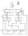
- the delay circuit according to the invention is shown schematically in Figure 1. It includes a primary circuit D1 with fixed delay.
- the D1 circuit receives the input signal e0 and outputs first and second intermediate signals m0 and ml.
- the signals m0 and m1 have between them a fixed delay T.
- the signals m0 and m1 are applied respectively to the inputs X and Y of a combination circuit C providing at output a combination signal f K.
- the combination circuit C comprises a control input CD receiving a command K representative of the weighting coefficients of the combination carried out by the circuit C.
- This command K is a function of a delay setpoint CN.
- the combination signal f K is applied to the input of a shaping circuit F whose output provides the output signal s K.
- a shaping circuit F whose output provides the output signal s K.
- the signal e0 arrives at the input E of the circuit on a first buffer memory (buffer in English literature) T1.
- a first buffer memory buffer in English literature
- three identical buffer memories T1, T2 and T3 are connected in series. They are used to introduce fixed delays to the e0 signal in series. Preferably the fixed delays are all equal to each other so that the signal e0 is delayed by T, 2T, 3T, etc. But the delays could be different from each other.
- the input of the first buffer memory is connected to one of the two inputs of a first MUX0 multiplexer.
- the output of the buffer memory T2 constitutes the other input of the multiplexer MUX0.
- the outputs of the buffer memories T1 and T3 are connected to the two inputs of a second multiplexer MUX1.
- the outputs of the multiplexers MUX0 and MUX1 are connected to the inputs of the combination circuit C performing delay interpolation.
- the output of the combination circuit leads the signal f K to the shaping circuit F.
- the combination circuit consists of two modules U0 and U1. Interpolation can thus be performed between either the signals e0 and r1, or the signals r2 and r1, or the signals r2 and r3. These three combinations are the only ones to have a constant delay equal to T between the signals.
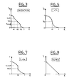
- the curves presented in FIGS. 2 to 9 make it possible to explain the operation of the circuit of FIG. 1. They explain the reasons which prevented the introduction of a simple circuit D1 with fixed delay equal to a time T 'greater than T which would have directly enlarged the delay range. They expose on the one hand the nature of the combination signals f K and of the output signals s K according to the comparison between the fixed delay time T between the signals m0 and m1 and a transition time tm.
- the transition time tm is the duration presented by the combination circuit for passing the signal Fk from its minimum value to its saturation value when K is 0 or 1.
- the figures show the variations of the delay t K in function of the coefficient K for different values of the transition time tm, the fixed delay T being assumed to be fixed.
- the timing diagram in FIG. 2a represents the signals m0 and m1 applied to the inputs X and Y of the circuit combination C.
- the signal m0 being a logic signal, it presents a steep transition front between a first and second level which is followed much more late from another unrepresented front restoring the signal at its first level.
- the falling front represents the end of the pulse of signal R0 which seeks to delay.
- the duration of this pulse is large compared to T, 2T, 3T ....
- the delayed signal m1 has been represented as a signal identical to m0 but delayed by a delay T defined by circuit D1. In practical, the edge of the signal m0 is used by the combination circuit at the moment when the signal m0 reaches a threshold value S1 of the combination C.
- the threshold value S1 corresponds to the average level between the minimum levels and maximum of signal m0. It is the same for the signal m1. In case the threshold value is set at medium level, these signals m0 and m1 could have a shape different from that shown.
- the delay T is defined as the time interval between instants when the signal m0 and the signal m1 reach the threshold value.
- the timing diagram of FIG. 2b represents the combination signal f K for different values of the weighting coefficient K.
- the integral of a pulse ends up being limited to the potential values anyway feed.
- the signal Fk is compared with a threshold value S2 preferably at the mean level between the maximum and the minimum of f k . At the moment when the comparator switches, the output signal is produced whose delay with respect to the signal e0 has been sought.
- the signal f1 corresponds to the case where K is equal to 1, i.e. when the weighting coefficient applied to signal m1 is zero.
- the signal has the form a trapezoid whose rising front begins at the moment zero corresponding to the instant when the signal m0 reaches a threshold value S1.
- the signal f1 increases so linear, the integration of a constant being a affine function, until the instant tm when it reaches a saturation level.
- the signal f0 corresponds to the case where the weighting coefficient K applied to the signal m0 is zero. This signal reproduces the signal f1 with the delay T.
- the combination signal has the shape represented by the curves f K1 and f K2 .
- the curve representing the combination signal then comprises three distinct parts Pa1, Pa2 and Pa3.
- the portion Pa1 corresponds to the time interval during which the signal m1 has not yet reached the threshold S1.
- the signal fki is then only proportional to the signal m0.
- the portion Pa3 of the curve representative of fki corresponds to the time interval from which the signal f1 reaches saturation.
- the signal fki is then only proportional to the signal m1.
- the portion Pa2 corresponds to the time interval between the arrival of the signal m1 at its threshold value and the arrival at saturation of fl.
- the signals f1 and f0 reach the value of the threshold S2 respectively at times t1 and t0 while the signal f Ki reaches this threshold at an instant ⁇ i .
- the difference between t1 and t0 is equal to the delay T.
- the respectively minimum and maximum delays of the combination signal with respect to the input signal are between t1 and t0 respectively. Consequently, the delay obtained in the general case will have a value ⁇ between t1 and t1 + T.
- the timing diagram in FIG. 2c represents the output signal from the shaping circuit F in each of the three cases represented in the timing diagram in FIG. 2b.
- the signals S1 and S0 have an edge respectively at times t1 and t0.
- the output signal s K will have a edge delayed by a value T K with respect to the signal S1, the value T K being between 0 and T, ie t1 + T with respect to mO.
- the value ⁇ obtained characteristic of the delay, varies as the cosine of the angle ⁇ 11 measuring the angle between the portion of the curve Pa1 and the horizontal.
- K2 tm / 2T.
- the portion Pa2 of the curve f K is parallel to f1 and f0; it is in fact the result of a linear combination of two parallel lines, the lines carrying the curves representative of f0 and fl. So for K between K1 and K2, the delay values ⁇ are the result of a linear function of K.
- FIGS 4 and 5 show the case where T equals tm.
- the values K1 and K2 defined above are equal, and the linear portion of the delay T K as a function of K has disappeared.
- the delay function T k assuming K as a variable, is therefore never linear.
- Figures 6 and 7 show the case where T is greater than tm.
- the portion Pa2 of the signal f K is horizontal, since it is the linear combination of F 1 and F 0 which are, over the interval considered to be horizontal. If K is equal to 1/2, this horizontal portion of f K is then located at the level of the transition threshold S2. The delay is then not perfectly defined, it is somewhere in the interval Z of the timing diagram C of FIG. 6, which creates a discontinuity at the level of the curve T K as a function of K, represented in FIG. 7.
- FIG. 8 and 9 show the case where T is less than tm / 2.
- the threshold S2 can only be reached with the portion Pa2 of the curve f K , therefore the response is necessarily linear as is visible in FIG. 9.
- the way in which the delay ⁇ varies as a function of the weighting coefficient K therefore essentially depends on the transition time tm defined above and on the fixed delay T.
- the transition time tm will define the minimum delay t1 of the output signal s K with respect to at the input signal e0. In the perfectly linear case such as that considered, this minimum delay is equal to half of the transition time.
- several delay circuits have been provided in series. For the delays existing between the combinations of signals e0 r1, r1 r2 and r2 r3, we will preferably choose values T less than tm. However, this is not an obligation. If necessary, we would lose a little linearity.
- T must preferably be less than tm to avoid any discontinuity of the delay T K as a function of the weighting coefficient K, therefore of the delay setpoint.
- a linear response of the delay T K is obtained as a function of K as soon as T is less than or equal to tm / 2.
- Figures 10 and 11 relate to an embodiment circuit diagram and in CMOS technology combination C.
- FIG. 10 is a schematic representation of a CMOS embodiment to facilitate its understanding.
- the circuit of FIG. 10 comprises a first and a second charge and discharge module U0, U1, of a common line L.
- the common line L is connected to a capacitor C1.
- the capacitor C1 is also connected to ground, or to another constant potential. The latter could even be Vdd, the operation of the circuit then being reversed.
- the potential of the common line is the measure of the combination signal.
- Each module U0, U1 has a PC charging circuit and a DC discharging circuit.
- Each PC load circuit includes a variable resistor RO * for the module U0, R1 * for the module U1, and a switch P0 for U0, P1 for U1.
- Each DC discharge circuit also includes a variable resistor R0 for U0, R1 for U1 and a switch N0 for U0 and N1 for U1.
- Each switch controls the connection by the resistance associated with it between line L and the supply potential Vdd for the charge circuit and Vss for the discharge circuit.
- the switches of the units U0 and U1 are controlled respectively by the signals m0 and m1 and their complement m0 * and m1 * .
- variable resistors R0, R0 * are controlled so as to take a value inversely proportional to the coefficient K, while the resistors R1, R1 * of the unit U1 are controlled so as to take a value inversely proportional to 1 - K.
- the potential of line L is the measure of the combination signal f K.
- the line L is charged with the potential Vdd and that the signals m0 and m1 are at zero.
- the switches P0 and P1 are then closed while the switches N0 and N1 are open.
- the switch N0 closes and the switch P0 opens.
- the circuit then has a time constant defined by the structural capacity at the level of line L and a resistance equivalent to the resistors R0 and R1 * connected in parallel. As R0 and R1 * are inversely proportional to K and 1 - K respectively, the time constant is independent of K.
- the line L will then discharge with this time constant from the value Vdd to the value (1 - K) Vdd .
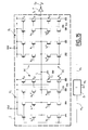
- FIG. 11 represents the detailed CMOS embodiment corresponding to the circuit of FIG. 10. It conforms to FIG. 2 described in French patent n ° 2 690 022.
- the PC charging and DC discharging circuits consist of MOS transistors respectively at channel P and N.
- the variable resistors R0, ..., R1 * are produced by means of MOS transistors connected in parallel and controlled by the signals K0, ... K i , and their complement K0 * , ..., K i * .
- the associated switches are constituted by the source drain paths of the MOS transistors whose gates receive the associated signal e0, e1.
- the structure capacity defining the time constant is due to the drain-gate capacity of the active MOS transistors connected to the line L.
- the resulting capacity remains constant, regardless of the value of K.
- the MOS transistors constituting the variable resistances of each charge or discharge circuit can be dimensioned so that their resistance varies according to a power of 2, according to the weights of the control signals K0, ..., K i ..., K0 * K i * .
- the delay circuit D1 connected to e0 at the input and which delivers the signals m0 and m1 as well as the shaping circuit F ensuring the transition from f K to S k .
- the capacitor C1 When the commands of the module U0 are validated, that is to say when all the k i are at 1, and that m0 is at 0, the capacitor C1 is loaded with a minimum delay. You can then change the k i to 0 when adjusting or programming. The values of k i are no longer modified when the delay to be imposed is determined. One activates, little by little according to the needs, branches of the module U1. The C1 capacity is still charging, but with a certain delay. Finally, when all the commands k i , are at 0, the current passes only through the module U1 and the delay is then maximum for the charging of the capacitor C1.
- the capacitor discharge phase follows the principle described above for the charge, with m0 and therefore a fortiori m1 equal to 1.
- capacitor C1 which is found at node L, is the potential of signal S K. It is only when this potential reaches the threshold of the shaping circuit F that the signal S K switches.
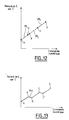
- Figure 12 shows a curve representing the delay between input E and output S of the circuit of the Figure 11 as a function of the digital control signal.
- Five characteristic points are visible on the curve.
- Point a corresponds to the minimum delay, therefore in case these are the signals e0 and r1 which enter into the combination circuit, with 100% of the current which goes into module U0.
- Point b corresponds to maximum delay when e0 and r1 enter the circuit combination with 100% of the current flowing in the module U1.
- the segment between a and b constitutes the range Pl1.
- This second range Pl2 ends with a point c which corresponds to the maximum delay between r1 and r2 with 100% of the current flowing through the U0 module.
- the advantage of recommended connection mode in fact does not switch than a multiplexer (MUX0) taking into account the symmetrical character of the circuit of FIGS. 11 and 15. Then it is the turn of the MUX1 multiplexer to switch, the signal r1 giving way to signal r3.
- MUX0 multiplexer
- Figures 14 and 15 show according to the invention a solution to this problem.
- FIG. 14 shows the circuit of Figure 10.
- These non-variable resistances no longer depend on K. They ensure that each module U0 and U1 contributes permanently to the charging or discharging of the line L.
- the advantage of such an assembly will be specified with the study of FIG. 15 which offers a more detailed description of this circuit.
- FIG. 15 shows the circuit of FIG. 11.
- the multiplexers MUX0 and MUX1 and the buffer memories T1, T2 and T3 constitute the delay circuit D1.
- a branch has been added in parallel. These branches each have in series two P-channel transistors in series and two N-channel transistors in series.
- the P channel transistors P01 and P02 for U0, P11 and P12 for U1 operate in the same way as the P channel transistors already present in the circuit shown in Figure 11 in the load circuits of U0 and U1.
- the new N channel transistors, N01 and N02 for U0, N11 and N12 for U1, intervene similarly in the discharge circuits of U0 and U1.
- the added transistors P01, N01, P11 and N11 which act as switches are always connected to the signals m0 and m1. But those which serve as variable resistors, namely P02, N02, P12 and N12, are permanently supplied: the transistors added to channel N, N02 and N12, are connected to the potential Vdd and the transistors added to channel P, P02 and P12 are related to the Vss potential. They do not depend on a K or K * command. Also, additional branches will always drive. This compensates for the leaks and the load distribution problems observed when switching the multiplexers, which result in a horizontal or slightly decreasing flat area.
- the current distributions in the modules U0 and U1 are slightly modified: we can no longer have 100% of the current flowing in one module and 0% in the other.
- each module typically comprises three transistors controlled by the commands K and K * .
- the added transistor which is permanently connected to the potential Vdd or Vss will typically be smaller than the other three transistors, so that there is a maximum of 90% of the current which can pass through a module U0 or U1. This means that the permanently supplied transistor must be three times smaller than the other transistors.
- transistors controlled by the coefficients K0, K1, etc ... have increasing grid widths binary (1, 2, 4, etc ).
- the transistor added in the additional branch has half grid width from the smallest of the previous grid widths.
- the branch added has a grid width half from that of other branches.
- FIGS 16a, 16b, 16c, 16d and 16e allow to explain what is happening now on the first beach. In their description, it will often be done reference to the circuit of figure 15.
- Figures 16a and 16b are the timing diagrams of the signals m0 and m1 offset by a time T.
- the origin of the time is defined when m0 switches to 0.
- the curves Co and Ci respectively correspond to the charge of the capacitor C1 before and after the introduction of the permanently connected transistors.
- the times t1 and ti are respectively the times taken, before and after the improvement of the invention, by the signal Sk to reach the threshold value S2. There is therefore at the start of the range a delay ti greater than t1. It can be seen in FIG. 16c that once m1 has switched to 0, the charge of the capacitor C1 is faster than before. This is explained by the fact that P11 then participates in the charge of C1.
- the new delay at the start of the track is greater than that in the absence of permanently connected branches, and there is less important at the end of the range.
- the points S1 and B1 are those of the new delay curve.
- the point S1 and B1 are respectively above and below points A and B above ( Figure 12).
- Figure 17 explains the change of range. She shows in dashes the real curve of the delays caused without improvement, a b b 'c c' d 'which is a broken line. The delay curve obtained with the improvement of the invention is shown in lines full. The latter goes through the points a1 b1 b'1 c1 it's 1 of 1 that are all aligned. The delay associated with point b1 is much lower than that associated with point b while the delay associated with point b'1 is greater to that associated with point b '.
- the digital control can therefore order more effectively the values of the coefficients ki and the tilting of the multiplexers. Indeed, if this command results from a slave action, the fact that the servo has a negative slope (b b ', c c ') and in particular a vertex, in b or in c, of the gain curve, causes this servo to oscillate around the value associated with point b.
- Figure 17 also shows the comparison between the delay curves obtained: the curve Co1 representative of the delay time in the absence of branches permanently connected, and the Co2 curve characteristic of the delay time for the circuit including branches permanently connected.
- the Co2 curve that we are approaching a optimal linearity; the delay is so anyway always increased.
Abstract
Description
L'invention concerne des circuits à retard variable, le retard étant réglable en fonction d'une consigne de retard. La consigne de retard peut prendre la forme d'une grandeur numérique.The invention relates to delay circuits. variable, the delay being adjustable according to a delay setpoint. The delay setpoint can take the form of a numerical quantity.
Les applications des circuits à retard variable sont nombreuses. Ces circuits à retard sont par exemple utilisés pour des ajustements de phase entre deux signaux logiques. Dans ce cas, un des deux signaux est appliqué à l'entrée d'un circuit à retard. Le réglage du retard du circuit à retard est alors commandé par la mesure du déphasage à compenser entre ces deux signaux logiques.Applications of variable delay circuits are numerous. These delay circuits are for example used for phase adjustments between two logic signals. In this case, one of the two signals is applied to the input of a delay circuit. Adjustment delay of the delay circuit is then controlled by the measurement of the phase shift to compensate between these two signals logical.
Un asservissement de phase peut être réalisé au moyen d'un signal de réglage analogique ou numérique. La solution numérique est souvent préférée car elle est moins sensible aux perturbations et aux atténuations dues à la transmission des signaux. De plus, dans le cas d'une réalisation sous forme de circuit intégré, elle est moins sensible aux dispersions de fabrication.Phase control can be performed at by means of an analog or digital adjustment signal. The digital solution is often preferred because it is less sensitive to disturbances and attenuations due to signal transmission. In addition, in the case of an implementation in the form of an integrated circuit, it is less sensitive to manufacturing dispersions.
Une première solution connue pour réaliser un circuit à retard à commande numérique consiste à utiliser un ensemble de portes élémentaires. Par exemple du type inverseur. L'ensemble des portes est associé à un système d'interconnexion, commandé numériquement, et permettant le branchement en cascade d'un nombre variable de portes élémentaires. L'application de ce type de circuit est cependant limitée aux cas où il n'est pas nécessaire d'obtenir une précision de réglage du retard inférieure au retard intrinsèque de la porte élémentaire. A first known solution for achieving a digitally controlled delay circuit consists of use a set of basic doors. Through example of the inverter type. The set of doors is associated with an interconnection system, controlled digitally, and allowing cascade connection of a variable number of elementary doors. The application of this type of circuit is however limited to cases where it is not necessary to obtain delay adjustment accuracy less than the delay intrinsic to the elementary door.
Une autre solution connue consiste à utiliser un circuit du type résistance-capacité où la résistance est constituée de plusieurs résistances élémentaires, branchées sélectivement en parallèle en fonction de la commande numérique. Dans ce cas, le retard est fixé par la constante de temps du circuit. Si toutes les résistances élémentaires ont la même valeur, le retard obtenu est alors inversement proportionnel au nombre de résistances sélectionnées. Or, pour obtenir une précision de réglage constante sur toute la plage de réglage, il est nécessaire que la fonction liant le retard à la grandeur numérique de réglage s'approche le plus possible d'une fonction linéaire.Another known solution is to use a resistance-capacity type circuit where resistance is made up of several elementary resistances, selectively connected in parallel according to the numerical control. In this case, the delay is fixed by the time constant of the circuit. If all elementary resistors have the same value, the delay obtained is then inversely proportional to the number of selected resistors. Now, to get a constant setting accuracy over the entire range of setting, it is necessary that the function linking the delay to the digital adjustment quantity approaches more of a linear function possible.
La réponse obtenue par la solution précédente est donc très éloignée de la relation linéaire puisqu'elle est de type hyperbolique. Pour se rapprocher de la réponse linéaire, il est alors nécessaire de dimensionner les résistances élémentaires à des valeurs bien précises et toutes différentes entre elles. Ce résultat est cependant très difficile à obtenir dans le cas d'une réalisation intégrée. D'autre part, il faudrait prévoir un tel circuit pour chaque signal que l'on veut ajuster en phase.The answer obtained by the previous solution is therefore very far from the linear relation since it is of hyperbolic type. To get closer to the linear response then it is necessary to dimension elementary resistances to values very precise and all different from each other. This result is however very difficult to obtain in the case of an integrated realization. On the other hand, such a circuit should be provided for each signal that we want to adjust in phase.
Si par exemple le circuit de retard est destiné à
être utilisé dans un circuit verrouillé en phase du
type décrit dans la demande de brevet européen publiée
sous le numéro 0 441 684, déposée le 30 janvier 1991 et
intitulé "Circuit verrouillé en phase et multiplieur de
fréquence en résultant", la solution précédente n'est
pas satisfaisante à cause de son encombrement et de sa
sensibilité aux dispersions de fabrication.If for example the delay circuit is intended to
be used in a circuit locked in phase of
type described in the published European patent application
under
L'invention a pour but de proposer un circuit à retard permettant un réglage précis, tout en assurant avec une approximation suffisante une réponse linéaire du retard en fonction de la consigne de retard, sur un intervalle de temps important, afin de s'approcher d'une précision de réglage constante.The object of the invention is to propose a circuit to delay allowing precise adjustment, while ensuring with sufficient approximation a linear response delay according to the delay setpoint, on a important time interval, in order to approach with constant adjustment precision.
Le brevet français publié sous le numéro 2 690 022
intitulé "Circuit à retard variable" présente un
circuit à retard variable assurant une réponse linéaire
du retard en fonction de la consigne de retard. Mais
l'amplitude de la plage de retard qu'il procure n'est
plus technologiquement satisfaisante.The French patent published under
En réponse à ce problème, un autre brevet publié en
France sous le numéro 2 689 339 intitulé "Procédé et
dispositif de réglage de retard à plusieurs gammes"
couvre le concept de multi-plages. Cependant, des
problèmes de linéarité du retard en fonction de la
consigne de retard sont observés dans la pratique.In response to this problem, another patent published in
France under
Le circuit de ce brevet a pour objet un circuit à retard pour fournir un signal de sortie présentant un retard par rapport à un signal d'entrée. Le retard est réglable en fonction d'une consigne de retard. Le circuit à retard comporte un circuit primaire, un circuit de combinaison et un circuit de mise en forme. Le circuit primaire reçoit le signal d'entrée et fournit deux signaux intermédiaires présentant entre eux un retard fixe. Le circuit de combinaison a deux entrées et comporte une entrée de commande recevant une grandeur de commande représentative de la consigne.The circuit of this patent relates to a circuit with delay to provide an output signal with a delay relative to an input signal. The delay is adjustable according to a delay setpoint. The delay circuit includes a primary circuit, a combination circuit and a shaping circuit. The primary circuit receives the input signal and provides two intermediate signals between them a fixed delay. The combination circuit has two inputs and has a command input receiving a control quantity representative of the setpoint.
Les signaux intermédiaires sont appliqués aux deux entrées du circuit de combinaison. Le circuit de combinaison fournit en sortie un signal de combinaison résultant d'une superposition avec une pondération et un effet d'intégration des signaux intermédiaires appliqués sur ses entrées. La pondération consiste à pondérer par un coefficient de pondération chacun des signaux en entrée du circuit de combinaison. Les valeurs des coefficients de pondération sont fonction de la grandeur de commande. Intermediate signals are applied to both combination circuit inputs. The circuit of combination outputs a combination signal resulting from an overlay with a weighting and an integration effect of intermediate signals applied to its inputs. Weighting consists of weight each of the signals at the input of the combination circuit. The weights values are a function of the order quantity.
Le signal de combinaison fourni par le circuit de combinaison est appliqué à l'entrée du circuit de mise en forme. Le circuit de mise en forme présente un effet de seuil. Le circuit de mise en forme produit un signal de déclenchement, le signal de sortie, lorsque le signal de combinaison, par effet d'intégration, atteint un seuil déterminé.The combination signal supplied by the combination is applied to the input of the bet circuit in shape. The shaping circuit has an effect threshold. The shaping circuit produces a signal trigger, the output signal, when the combination signal reached by integration effect a determined threshold.
Ainsi, le retard effectif du signal de sortie par rapport au signal d'entrée est dépendant du niveau du signal de combinaison. Il est souhaitable que les amplitudes maximum et minimum du signal de combinaison soient indépendantes de la consigne de retard. Dans ce but, la somme des deux coefficients de pondération est constante.Thus, the effective delay of the output signal by relation to the input signal is dependent on the level of combination signal. It is desirable that maximum and minimum amplitudes of the combination signal are independent of the delay setpoint. In this goal, the sum of the two weights is constant.
En pratique, l'intégration dans le circuit de combinaison est produite par un intégrateur ou un circuit à constante de temps présentant toujours un effet de saturation définissant les niveaux extrêmes du signal de combinaison.In practice, integration into the combination is produced by an integrator or a time constant circuit always presenting a saturation effect defining the extreme levels of combination signal.
Un temps de transition est défini comme l'intervalle de temps pendant lequel le signal de combinaison varie selon une fonction linéaire ou quasi-linéaire lorsqu'un des coefficients de pondération associés aux signaux intermédiaires est nul.A transition time is defined as the time interval during which the signal combination varies according to a linear function or quasi-linear when one of the coefficients of weighting associated with the intermediate signals is no.
Le fait d'imposer un retard fixe inférieur au temps de transition assure que le retard du signal de sortie par rapport au signal d'entrée ne présente pas de discontinuité en fonction des coefficients de pondération. Pour que la variation du retard en fonction de la consigne de retard varie sur toute la plage de réglage selon une fonction pratiquement linéaire de la consigne, le circuit de combinaison et/ou le circuit primaire à retard fixe pourront être dimensionnés de façon à ce que le retard fixe soit égal à la moitié du temps de transition.Imposing a fixed delay less than the time transition ensures that the delay of the output signal with respect to the input signal has no discontinuity as a function of the coefficients of weighting. So that the variation of the delay in delay setpoint function varies over the entire setting range depending on a function practically setpoint linear, the combination circuit and / or the fixed delay primary circuit may be dimensioned so that the fixed delay is equal halfway through the transition time.
C'est cette contrainte liant le retard fixe et le temps de transition qui empêche d'élargir l'amplitude de la plage de retard à partir du circuit décrit dans le brevet 2 690 022 mentionné ci-dessus. En effet, la plage de retard est définie par le circuit à retard fixe. Or si on augmente ce retard fixe, on ne répond plus à la condition imposant un retard fixe égal à la moitié du temps de transition. Cette condition assure la linéarité du retard du signal de sortie par rapport à la consigne d'entrée. Pour résoudre ce problème, dans le brevet 2 689 339, on modifie le circuit primaire. On y réalise un jeu de circuit de retards en cascade. On connecte les sorties de ces circuits de retard en cascade à un multiplexeur. Avec le multiplexeur on sélectionne, à titre de signaux intermédiaires, des couples de signaux possédant entre eux un retard fixe (comme avant) et, ensemble, un retard de base par rapport au signal d'entrée. Dans ce cas, au moment du saut de gamme, on constate des discontinuités technologiques de retard. Si la discontinuité est négative, elle engendre une impossibilité pour l'asservissement de trouver un réglage équilibré à une valeur acceptable. Dans l'invention, on remédie à ce problème en modifiant le circuit de combinaison de façon, en pratique, à ce qu'il ne permette pas d'explorer toute une plage.It is this constraint linking the fixed delay and the transition time which prevents the amplitude from widening the delay range from the circuit described in the patent 2,690,022 mentioned above. Indeed, the delay range is defined by the delay circuit fixed. However if we increase this fixed delay, we do not respond plus on condition imposing a fixed delay equal to the half the transition time. This condition ensures the linearity of the delay of the output signal with respect to to the entry setpoint. To resolve this problem, in Patent 2,689,339, the primary circuit is modified. We there realizes a cascade delay circuit game. We connect the outputs of these delay circuits in cascade to a multiplexer. With the multiplexer we selects, as intermediate signals, signal pairs with a fixed delay between them (as before) and, together, a basic delay by relative to the input signal. In this case, at the time of range jump, there are discontinuities delay technology. If the discontinuity is negative, it creates an impossibility for the enslavement of finding a balanced setting at a acceptable value. In the invention, this is remedied problem by modifying the combination circuit of way, in practice, that it does not allow to explore a whole beach.
L'invention a donc pour objet un circuit à retard pour fournir un signal de sortie présentant un retard par rapport à un signal d'entrée, le retard étant réglable en fonction d'une consigne de retard, le circuit à retard comportant
- un circuit primaire, recevant le signal d'entrée et fournissant des premier et second signaux intermédiaires présentant entre eux un retard fixe,
- un circuit de combinaison à deux entrées, fournissant en sortie un signal de combinaison résultant d'une superposition avec une pondération fonction de la grandeur de commande et un effet d'intégration des signaux appliqués sur ses entrées, les signaux intermédiaires étant appliqués aux deux entrées du circuit de combinaison,
- un circuit de mise en forme recevant le signal de combinaison, fournissant le signal de sortie, et présentant un effet de seuil,
- une entrée de commande recevant une grandeur de commande représentative de la consigne,
- une ligne commune avec un condensateur relié à cette ligne commune et à un potentiel d'alimentation,
- un premier et un second module de charge et décharge de la ligne commune commandés respectivement par les premier et second signaux intermédiaires, le potentiel de la ligne commune constituant la mesure du signal de combinaison,
- a primary circuit, receiving the input signal and supplying first and second intermediate signals having a fixed delay between them,
- a combination circuit with two inputs, providing as output a combination signal resulting from a superposition with a weighting depending on the control quantity and an integration effect of the signals applied to its inputs, the intermediate signals being applied to the two inputs the combination circuit,
- a shaping circuit receiving the combination signal, supplying the output signal, and having a threshold effect,
- a control input receiving a control quantity representative of the setpoint,
- a common line with a capacitor connected to this common line and to a supply potential,
- a first and a second module for charging and discharging the common line controlled respectively by the first and second intermediate signals, the potential of the common line constituting the measurement of the combination signal,
L'invention a également pour objet un mode de réalisation spécialement conçu pour pouvoir utiliser la technologie CMOS. Cette réalisation, ainsi que d'autres aspects et avantages de l'invention, apparaítront dans la suite de la description en références aux figures, qui ne sont données qu'à titre indicatif et nullement limitatif de l'invention. Les figures montrent:
- la figure 1 représente le schéma de principe d'un circuit à retard variable à plusieurs plages de retard;
- les figures 2a à 2c, 4a à 4c, 6a à 6c et 8a à 8c présentent des chronogrammes permettant d'expliquer le fonctionnement du circuit de la figure 1;
- les figures 3, 5, 7, 9 montrent les variations du retard en fonction de la grandeur de commande pour différents dimensionnements du circuit de la figure 1;
- la figure 10 représente le schéma de principe d'une réalisation CMOS d'un circuit à retard variable à plusieurs plages de retard;
- la figure 11 représente une réalisation détaillée en technologie CMOS du circuit à retard variable à plusieurs plages de retard;
- la figure 12 présente une courbe théorique représentant des temps de retard en fonction de la commande numérique;
- la figure 13 montre une courbe représentant les temps de retard effectivement observés dans le circuit à retard variable à plusieurs plages de retard en fonction de la commande numérique;
- la figure 14 représente l'amélioration amenée par l'invention du circuit présenté à la figure 10 conduisant à une amélioration de la linéarité du retard en fonction de la commande numérique;
- la figure 15 représente l'amélioration amenée par l'invention du circuit présenté à la figure 11 conduisant à une amélioration de la linéarité du retard en fonction de la commande numérique;
- la figure 16 présente une comparaison, sur une plage, des temps de retard obtenus en fonction de la commande numérique, avec les circuits des figures 11 et 15;
- la figure 17 présente une comparaison entre des temps de retard obtenus avec le circuit de la figure 11 et ceux obtenus avec le circuit de la figure 15.
- FIG. 1 represents the block diagram of a variable delay circuit with several delay ranges;
- Figures 2a to 2c, 4a to 4c, 6a to 6c and 8a to 8c show timing diagrams to explain the operation of the circuit of Figure 1;
- Figures 3, 5, 7, 9 show the variations of the delay as a function of the control quantity for different dimensions of the circuit of Figure 1;
- FIG. 10 represents the block diagram of a CMOS embodiment of a variable delay circuit with several delay ranges;
- FIG. 11 represents a detailed embodiment in CMOS technology of the variable delay circuit with several delay ranges;
- FIG. 12 presents a theoretical curve representing delay times as a function of the digital control;
- FIG. 13 shows a curve representing the delay times actually observed in the variable delay circuit with several delay ranges as a function of the digital control;
- FIG. 14 represents the improvement brought about by the invention of the circuit presented in FIG. 10 leading to an improvement in the linearity of the delay as a function of the digital control;
- FIG. 15 represents the improvement brought about by the invention of the circuit presented in FIG. 11 leading to an improvement in the linearity of the delay as a function of the digital control;
- FIG. 16 shows a comparison, over a range, of the delay times obtained as a function of the digital control, with the circuits of FIGS. 11 and 15;
- FIG. 17 presents a comparison between delay times obtained with the circuit of FIG. 11 and those obtained with the circuit of FIG. 15.
Le circuit de retard selon l'invention est représenté schématiquement à la figure 1. Il comporte un circuit primaire D1 à retard fixe. Le circuit D1 reçoit le signal d'entrée e0 et fournit en sortie des premier et deuxième signaux intermédiaire m0 et ml.The delay circuit according to the invention is shown schematically in Figure 1. It includes a primary circuit D1 with fixed delay. The D1 circuit receives the input signal e0 and outputs first and second intermediate signals m0 and ml.
Les signaux m0 et m1 présentent entre eux un retard fixe T. Les signaux m0 et m1 sont appliqués respectivement aux entrées X et Y d'un circuit de combinaison C fournissant en sortie un signal de combinaison fK. Le circuit de combinaison C comporte une entrée de commande CD recevant une commande K représentative des coefficients de pondération de la combinaison effectuée par le circuit C. Cette commande K est fonction d'une consigne de retard CN.The signals m0 and m1 have between them a fixed delay T. The signals m0 and m1 are applied respectively to the inputs X and Y of a combination circuit C providing at output a combination signal f K. The combination circuit C comprises a control input CD receiving a command K representative of the weighting coefficients of the combination carried out by the circuit C. This command K is a function of a delay setpoint CN.
Le signal de combinaison fK est appliqué à l'entrée d'un circuit de mise en forme F dont la sortie fournit le signal de sortie sK. Pour simplifier la suite de l'exposé, on raisonnera sur les grandeurs normalisées des signaux impliqués et on supposera que les coefficients de pondération affectés aux signaux m0 et m1 sont respectivement les valeurs K et 1 - K, avec K compris entre 0 et 1.The combination signal f K is applied to the input of a shaping circuit F whose output provides the output signal s K. To simplify the rest of the presentation, we will reason on the normalized quantities of the signals involved and we will assume that the weighting coefficients assigned to the signals m0 and m1 are respectively the values K and 1 - K, with K between 0 and 1.
Dans ces conditions, le circuit C est conçu pour réaliser la combinaison gK = K.m0 + (1 - K).m1 avec intégration par rapport au temps pour obtenir fk à partir de gk.Under these conditions, circuit C is designed to perform the combination g K = K.m0 + (1 - K) .m1 with integration with respect to time to obtain f k from g k .
Le signal e0 arrive à l'entrée E du circuit sur une première mémoire tampon (buffer dans la littérature anglaise) T1. Dans l'exemple préféré représenté, trois mémoires tampons identiques T1, T2 et T3 sont montés en série. Elles servent à introduire en série des retards fixes au signal e0. De préférence les retards fixes sont tous égaux entre eux à T de sorte que le signal e0 soit retardé de T, 2T, 3T, etc... Mais les retards pourraient être différents les uns des autres. On trouve le signal r1 à la sortie de la mémoire tampon T1, le signal r2 à la sortie de la mémoire tampon T2, le signal r3 à la sortie de la mémoire tampon T3. L'entrée de la première mémoire tampon est connectée à l'une des deux entrées d'un premier multiplexeur MUX0. La sortie de la mémoire tampon T2 constitue l'autre entrée du multiplexeur MUX0. Les sorties des mémoires tampons T1 et T3 sont connectées aux deux entrées d'un second multiplexeur MUX1. Les sorties des multiplexeurs MUX0 et MUX1 sont connectées aux entrées du circuit de combinaison C réalisant une interpolation de retard. La sortie du circuit de combinaison conduit le signal fK au circuit de mise en forme F. Le circuit de combinaison est constitué de deux modules U0 et U1. L'interpolation peut ainsi être réalisée entre soit les signaux e0 et r1, soit les signaux r2 et r1, soit les signaux r2 et r3. Ces trois combinaisons sont les seules à présenter un retard constant égal à T entre les signaux. En présentant les signaux de ces trois combinaisons de signaux à l'entrée du circuit de combinaison, on est certain d'obtenir une plage de retard constante. La combinaison des signaux e0 et r3 ne sera jamais appliquée à l'entrée du circuit de combinaison, car le retard entre les deux signaux serait trop important et ne satisferait pas aux conditions de linéarité évoquées précédemment.The signal e0 arrives at the input E of the circuit on a first buffer memory (buffer in English literature) T1. In the preferred example shown, three identical buffer memories T1, T2 and T3 are connected in series. They are used to introduce fixed delays to the e0 signal in series. Preferably the fixed delays are all equal to each other so that the signal e0 is delayed by T, 2T, 3T, etc. But the delays could be different from each other. We find the signal r1 at the output of the buffer memory T1, the signal r2 at the output of the buffer memory T2, the signal r3 at the output of the buffer memory T3. The input of the first buffer memory is connected to one of the two inputs of a first MUX0 multiplexer. The output of the buffer memory T2 constitutes the other input of the multiplexer MUX0. The outputs of the buffer memories T1 and T3 are connected to the two inputs of a second multiplexer MUX1. The outputs of the multiplexers MUX0 and MUX1 are connected to the inputs of the combination circuit C performing delay interpolation. The output of the combination circuit leads the signal f K to the shaping circuit F. The combination circuit consists of two modules U0 and U1. Interpolation can thus be performed between either the signals e0 and r1, or the signals r2 and r1, or the signals r2 and r3. These three combinations are the only ones to have a constant delay equal to T between the signals. By presenting the signals of these three combinations of signals at the input of the combination circuit, it is certain to obtain a constant delay range. The combination of signals e0 and r3 will never be applied to the input of the combination circuit, because the delay between the two signals would be too great and would not satisfy the linearity conditions mentioned above.
On peut ainsi mettre à la suite plusieurs plages de retard. La mise à la suite consiste à utiliser une première combinaison e0 r1 pour produire un retard variable entre 0 et T, à utiliser une deuxième combinaison r1 r2 pour produire un retard variable entre T et 2T, à utiliser une troisième combinaison r2 r3 pour produire un retard variable entre 2T et 3T et ainsi de suite, le nombre de mémoires tampons utilisées et la capacité des multiplexeurs conditionnant la dynamique totale de retard des circuits de retard de l'invention.We can thus put several ranges of delay. The following is to use a first combination e0 r1 to produce a delay variable between 0 and T, use a second combination r1 r2 to produce a variable delay between T and 2T, use a third combination r2 r3 to produce a variable delay between 2T and 3T and so on, the number of buffers used and the capacity of the multiplexers conditioning the total delay dynamics of delay circuits the invention.
Les courbes présentés aux figures 2 à 9 permettent d'expliquer le fonctionnement du circuit de la figure 1. Elles explicitent les raisons qui ont empêché d'introduire un circuit D1 simple à retard fixe égal à un temps T' supérieur à T qui aurait directement agrandi la plage de retard. Elles exposent d'une part la nature des signaux de combinaison fK et des signaux de sortie sK selon la comparaison entre le temps de retard fixe T entre les signaux m0 et m1 et un temps de transition tm. Le temps de transition tm est la durée présentée par le circuit de combinaison pour faire passer le signal Fk de sa valeur minimum à sa valeur de saturation lorsque K vaut 0 ou 1. D'autre part les figures montrent les variations du retard tK en fonction du coefficient K pour différentes valeurs du temps de transition tm, le retard fixe T étant supposé fixé.The curves presented in FIGS. 2 to 9 make it possible to explain the operation of the circuit of FIG. 1. They explain the reasons which prevented the introduction of a simple circuit D1 with fixed delay equal to a time T 'greater than T which would have directly enlarged the delay range. They expose on the one hand the nature of the combination signals f K and of the output signals s K according to the comparison between the fixed delay time T between the signals m0 and m1 and a transition time tm. The transition time tm is the duration presented by the combination circuit for passing the signal Fk from its minimum value to its saturation value when K is 0 or 1. On the other hand the figures show the variations of the delay t K in function of the coefficient K for different values of the transition time tm, the fixed delay T being assumed to be fixed.
Le cas où T est compris entre tm/2 et tm est représenté figures 2 et 3.The case where T is between tm / 2 and tm is shown in Figures 2 and 3.
Le chronogramme figure 2a représente les signaux m0 et m1 appliqués aux entrées X et Y du circuit de combinaison C. Le signal m0 étant un signal logique, il présente un front raide de transition entre un premier et un second niveau qui est suivi bien plus tard d'un autre front non-représenté rétablissant le signal à son premier niveau. Le front descendant représente la fin de l'impulsion du signal R0 qu'on cherche à retarder. La durée de cette impulsion est grande par rapport à T, 2T, 3T ... . Le signal retardé m1 a été représenté comme un signal identique à m0 mais retardé d'un retard T défini par le circuit D1. En pratique, le front du signal m0 est exploité par le circuit de combinaison à l'instant où le signal m0 atteint une valeur de seuil S1 du circuit de combinaison C. En général, la valeur de seuil S1 correspond au niveau moyen entre les niveaux minimum et maximum du signal m0. Il en est de même pour le signal m1. Dans le cas ou la valeur de seuil est réglée au niveau moyen, ces signaux m0 et m1 pourraient avoir une forme différente de celle représentée. Le retard T est défini comme l'intervalle de temps séparant les instants où le signal m0 et le signal m1 atteignent la valeur de seuil.The timing diagram in FIG. 2a represents the signals m0 and m1 applied to the inputs X and Y of the circuit combination C. The signal m0 being a logic signal, it presents a steep transition front between a first and second level which is followed much more late from another unrepresented front restoring the signal at its first level. The falling front represents the end of the pulse of signal R0 which seeks to delay. The duration of this pulse is large compared to T, 2T, 3T .... The delayed signal m1 has been represented as a signal identical to m0 but delayed by a delay T defined by circuit D1. In practical, the edge of the signal m0 is used by the combination circuit at the moment when the signal m0 reaches a threshold value S1 of the combination C. In general, the threshold value S1 corresponds to the average level between the minimum levels and maximum of signal m0. It is the same for the signal m1. In case the threshold value is set at medium level, these signals m0 and m1 could have a shape different from that shown. The delay T is defined as the time interval between instants when the signal m0 and the signal m1 reach the threshold value.
Le chronogramme de la figure 2b représente le signal de combinaison fK pour différentes valeurs du coefficient de pondération K. Bien entendu, la forme des signaux représentés est une représentation simplifiée des signaux qu'on peut obtenir avec des circuits réels. Il convient toutefois de noter que cette représentation n'est pas éloignée de la réalité. En particulier, on observera toujours un palier de saturation. Ceci est montré sur la courbe f1 (K = 1) à partir de t = tm et sur les autres courbes à partir de t = tm + T. L'intégrale d'une impulsion finit de toutes façons par être limitée aux valeurs du potentiel d'alimentation. Dans le circuit F de mise en forme le signal Fk est comparé à une valeur de seuil S2 de préférence au niveau moyen entre le maximum et le minimum de fk. Au moment ou le comparateur bascule on produit le signal de sortie dont le retard par rapport au signal e0 a été recherché.The timing diagram of FIG. 2b represents the combination signal f K for different values of the weighting coefficient K. Of course, the shape of the signals represented is a simplified representation of the signals that can be obtained with real circuits. However, it should be noted that this representation is not far from reality. In particular, we will always observe a level of saturation. This is shown on the curve f1 (K = 1) from t = tm and on the other curves from t = tm + T. The integral of a pulse ends up being limited to the potential values anyway feed. In the shaping circuit F the signal Fk is compared with a threshold value S2 preferably at the mean level between the maximum and the minimum of f k . At the moment when the comparator switches, the output signal is produced whose delay with respect to the signal e0 has been sought.
Le signal f1 correspond au cas où K est égal à 1, c'est-à-dire lorsque le coefficient de pondération appliqué au signal m1 est nul. Le signal a la forme d'un trapèze dont le front montant débute à l'instant zéro correspondant à l'instant où le signal m0 atteint une valeur de seuil S1. Le signal f1 augmente de façon linéaire, l'intégration d'une constante étant une fonction affine, jusqu'à l'instant tm où il atteint un palier de saturation.The signal f1 corresponds to the case where K is equal to 1, i.e. when the weighting coefficient applied to signal m1 is zero. The signal has the form a trapezoid whose rising front begins at the moment zero corresponding to the instant when the signal m0 reaches a threshold value S1. The signal f1 increases so linear, the integration of a constant being a affine function, until the instant tm when it reaches a saturation level.
Le signal f0 correspond au cas où le coefficient de pondération K appliqué au signal m0 est nul. Ce signal reproduit le signal f1 avec le retard T. Pour des coefficients de pondération différents de ces deux cas extrêmes, le signal de combinaison a l'allure représentée par les courbes fK1 et fK2. La courbe représentative du signal de combinaison comporte alors trois parties distinctes Pa1, Pa2 et Pa3. La portion Pa1 correspond à l'intervalle de temps pendant lequel le signal m1 n'a pas encore atteint le seuil S1. Le signal fki est alors uniquement proportionnel au signal m0. La portion Pa3 de la courbe représentative de fki correspond à l'intervalle de temps à partir duquel le signal f1 arrive à saturation. Le signal fki est alors uniquement proportionnel au signal m1. La portion Pa2 correspond à l'intervalle de temps entre l'arrivée du signal m1 à sa valeur seuil et l'arrivée à saturation de fl. Les signaux f1 et f0 atteignent la valeur du seuil S2 respectivement aux instants t1 et t0 tandis que le signal fKi atteint ce seuil à un instant Θi. L'écart entre t1 et t0 est égal au retard T. Ainsi, les retards respectivement minimum et maximum du signal de combinaison par rapport au signal d'entrée sont compris entre respectivement t1 et t0. Par conséquent, le retard obtenu dans le cas général aura une valeur Θ comprise entre t1 et t1 + T.The signal f0 corresponds to the case where the weighting coefficient K applied to the signal m0 is zero. This signal reproduces the signal f1 with the delay T. For weighting coefficients different from these two extreme cases, the combination signal has the shape represented by the curves f K1 and f K2 . The curve representing the combination signal then comprises three distinct parts Pa1, Pa2 and Pa3. The portion Pa1 corresponds to the time interval during which the signal m1 has not yet reached the threshold S1. The signal fki is then only proportional to the signal m0. The portion Pa3 of the curve representative of fki corresponds to the time interval from which the signal f1 reaches saturation. The signal fki is then only proportional to the signal m1. The portion Pa2 corresponds to the time interval between the arrival of the signal m1 at its threshold value and the arrival at saturation of fl. The signals f1 and f0 reach the value of the threshold S2 respectively at times t1 and t0 while the signal f Ki reaches this threshold at an instant Θ i . The difference between t1 and t0 is equal to the delay T. Thus, the respectively minimum and maximum delays of the combination signal with respect to the input signal are between t1 and t0 respectively. Consequently, the delay obtained in the general case will have a value Θ between t1 and t1 + T.
Le chronogramme de la figure 2c représente le signal de sortie du circuit de mise en forme F dans chacun des trois cas représentés sur le chronogramme de la figure 2b. Ainsi, les signaux S1 et S0 présentent un front respectivement aux instants t1 et t0. Pour un coefficient K donné, le signal de sortie sK possédera un front retardé d'une valeur TK par rapport aux signal S1, la valeur TK étant comprise entre 0 et T, soit t1 + T par rapport à mO.The timing diagram in FIG. 2c represents the output signal from the shaping circuit F in each of the three cases represented in the timing diagram in FIG. 2b. Thus, the signals S1 and S0 have an edge respectively at times t1 and t0. For a given coefficient K, the output signal s K will have a edge delayed by a value T K with respect to the signal S1, the value T K being between 0 and T, ie t1 + T with respect to mO.
Sur la figure 3, on voit que pour K compris entre 0 et une première valeur K1, TK varie entre T et tm/2 selon une sinusoïde. Cette première valeur K1 correspond au coefficient 1- K facteur de m1, qui coïncide avec un retard Θ égal à tm. Pour K compris entre Θ et K1, la valeur Θ obtenue, caractéristique du retard, varie en effet comme le cosinus d'un angle α2 mesurant l'angle entre la portion Pa3 de la courbe fK et l'horizontale. Le calcul permet de vérifier facilement que K1 est égal à 1 - tm/2T, par exemple en établissant une équation de la droite contenant la portion de courbe Pa3.In Figure 3, we see that for K between 0 and a first value K1, T K varies between T and tm / 2 according to a sinusoid. This first value K1 corresponds to the coefficient 1- K factor of m1, which coincides with a delay Θ equal to tm. For K between Θ and K1, the value Θ obtained, characteristic of the delay, varies in effect as the cosine of an angle α2 measuring the angle between the portion Pa3 of the curve f K and the horizontal. The calculation makes it easy to verify that K1 is equal to 1 - tm / 2T, for example by establishing an equation of the line containing the portion of curve Pa3.
De même, pour K compris entre K2 et 1, la valeur Θ obtenue, caractéristique du retard, varie comme le cosinus de l'angle α11 mesurant l'angle entre la portion de courbe Pa1 et l'horizontale. De la même façon qu'on a calculé K1, on peut calculer K2 = tm/2T. Entre K1 et K2, la portion Pa2 de la courbe fK est parallèle à f1 et f0; elle est en effet le résultat d'une combinaison linéaire de deux droites parallèles, les droites porteuses des courbes représentatives de f0 et fl. Donc pour K compris entre K1 et K2, les valeurs de retard Θ sont le résultat d'une fonction linéaire de K.Similarly, for K between K2 and 1, the value Θ obtained, characteristic of the delay, varies as the cosine of the angle α11 measuring the angle between the portion of the curve Pa1 and the horizontal. In the same way that we calculated K1, we can calculate K2 = tm / 2T. Between K1 and K2, the portion Pa2 of the curve f K is parallel to f1 and f0; it is in fact the result of a linear combination of two parallel lines, the lines carrying the curves representative of f0 and fl. So for K between K1 and K2, the delay values Θ are the result of a linear function of K.
Les figures 4 et 5 représentent le cas où T égal tm. Dans ce cas, les valeurs K1 et K2 définies précédemment sont égales, et la portion linéaire du retard TK en fonction de K a disparu. La fonction de retard Tk, admettant K comme variable, n'est alors jamais linéaire.Figures 4 and 5 show the case where T equals tm. In this case, the values K1 and K2 defined above are equal, and the linear portion of the delay T K as a function of K has disappeared. The delay function T k , assuming K as a variable, is therefore never linear.
Les figures 6 et 7 représentent le cas où T est supérieur à tm. Dans ce cas, la portion Pa2 du signal fK est horizontale, car elle est la combinaison linéaire de F1 et F0 qui sont, sur l'intervalle considéré horizontales. Si K est égal à 1/2, cette portion horizontale de fK se situe alors au niveau du seuil de transition S2. Le retard n'est alors pas parfaitement défini, il est quelque part dans l'intervalle Z du chronogramme C de la figure 6, ce qui crée une discontinuité au niveau de la courbe TK en fonction de K, représentée figure 7.Figures 6 and 7 show the case where T is greater than tm. In this case, the portion Pa2 of the signal f K is horizontal, since it is the linear combination of F 1 and F 0 which are, over the interval considered to be horizontal. If K is equal to 1/2, this horizontal portion of f K is then located at the level of the transition threshold S2. The delay is then not perfectly defined, it is somewhere in the interval Z of the timing diagram C of FIG. 6, which creates a discontinuity at the level of the curve T K as a function of K, represented in FIG. 7.
Les figures 8 et 9 représentent le cas où T est inférieur à tm/2. Dans ce cas, le seuil S2 ne peut être atteint qu'avec la portion Pa2 de la courbe fK, donc la réponse est nécessairement linéaire comme c'est visible sur la figure 9.Figures 8 and 9 show the case where T is less than tm / 2. In this case, the threshold S2 can only be reached with the portion Pa2 of the curve f K , therefore the response is necessarily linear as is visible in FIG. 9.
La façon dont le retard Θ varie en fonction du coefficient de pondération K dépend donc essentiellement du temps de transition tm défini ci-dessus et du retard fixe T. Le temps de transition tm définira le retard minimum t1 du signal de sortie sK par rapport au signal d'entrée e0. Dans le cas parfaitement linéaire tel que celui considéré, ce retard minimum est égal à la moitié du temps de transition. Dans l'invention, pour résoudre le problème de durée du retard on a prévu plusieurs circuits de retard en série. Pour les retards existant entre les combinaisons de signaux e0 r1, r1 r2 et r2 r3, on choisira de préférence des valeurs T inférieures à tm. Cependant, ce n'est pas une obligation. On perdrait le cas échéant un peu de linéarité.The way in which the delay Θ varies as a function of the weighting coefficient K therefore essentially depends on the transition time tm defined above and on the fixed delay T. The transition time tm will define the minimum delay t1 of the output signal s K with respect to at the input signal e0. In the perfectly linear case such as that considered, this minimum delay is equal to half of the transition time. In the invention, to solve the delay duration problem, several delay circuits have been provided in series. For the delays existing between the combinations of signals e0 r1, r1 r2 and r2 r3, we will preferably choose values T less than tm. However, this is not an obligation. If necessary, we would lose a little linearity.
L'analyse précédente permet de tirer quelques conclusions concernant le dimensionnement à apporter au circuit primaire et au circuit de combinaison. Il apparaít tout d'abord que T doit de préférence être inférieur à tm pour éviter toute discontinuité du retard TK en fonction du coefficient de pondération K, donc de la consigne de retard. D'autre part on obtient une réponse linéaire du retard TK en fonction de K dès que T est inférieur ou égal à tm/2. Ainsi, pour tm fixé, on obtiendra une réponse linéaire tout en ayant la plus grande plage de réglage lorsque T est égal à tm/2.The previous analysis allows to draw some conclusions concerning the dimensioning to bring to the primary circuit and to the combination circuit. It appears first of all that T must preferably be less than tm to avoid any discontinuity of the delay T K as a function of the weighting coefficient K, therefore of the delay setpoint. On the other hand, a linear response of the delay T K is obtained as a function of K as soon as T is less than or equal to tm / 2. Thus, for fixed tm, we will obtain a linear response while having the largest adjustment range when T is equal to tm / 2.
Le retard fixe T détermine la plage de réglage du retard. Aussi, pour une plage déterminée, il sera toujours possible d'obtenir une réponse linéaire en choisissant tm = 2T. On pourra cependant être amené à choisir un temps de transition inférieur afin de réduire le retard minimal t1 qui dépend directement du temps de transition tm. D'une façon générale, le choix de T et de tm résultera d'un compromis entre le retard minimal, la plage de réglage et la linéarité du retard par rapport à la consigne de retard.The fixed delay T determines the adjustment range of the delay. Also, for a specific range, it will be always possible to get a linear response in choosing tm = 2T. We may however be led to choose a lower transition time in order to reduce the minimum delay t1 which directly depends on the transition time tm. Generally speaking, the choice of T and tm will result from a compromise between the delay minimum, the adjustment range and the linearity of the delay compared to the delay setpoint.
Les figures 10 et 11 concernent une réalisation schématique et en technologie CMOS du circuit de combinaison C.Figures 10 and 11 relate to an embodiment circuit diagram and in CMOS technology combination C.
La figure 10 est la représentation schématique d'une réalisation CMOS permettant de faciliter sa compréhension. Le circuit de la figure 10 comporte un premier et un second module de charge et décharge U0, U1, d'une ligne commune L. La ligne commune L est reliée à un condensateur C1. Le condensateur C1 est par ailleurs relié à la masse, ou a un autre potentiel constant. Ce dernier pourrait même être Vdd, le fonctionnement du circuit étant alors inversé. Le potentiel de la ligne commune constitue la mesure du signal de combinaison. Chaque module U0, U1 comporte un circuit de charge PC et un circuit de décharge DC. Chaque circuit de charge PC comporte une résistance variable RO* pour le module U0, R1* pour le module U1, et un interrupteur P0 pour U0, P1 pour U1. Chaque circuit de décharge DC comporte également une résistance variable R0 pour U0, R1 pour U1 et un interrupteur N0 pour U0 et N1 pour U1. Chaque interrupteur contrôle la connexion par la résistance qui lui est associée entre la ligne L et le potentiel d'alimentation Vdd pour le circuit de charge et Vss pour le circuit de décharge. Les interrupteurs des unités U0 et U1 sont commandés respectivement par les signaux m0 et m1 et leur complément m0* et m1*.Figure 10 is a schematic representation of a CMOS embodiment to facilitate its understanding. The circuit of FIG. 10 comprises a first and a second charge and discharge module U0, U1, of a common line L. The common line L is connected to a capacitor C1. The capacitor C1 is also connected to ground, or to another constant potential. The latter could even be Vdd, the operation of the circuit then being reversed. The potential of the common line is the measure of the combination signal. Each module U0, U1 has a PC charging circuit and a DC discharging circuit. Each PC load circuit includes a variable resistor RO * for the module U0, R1 * for the module U1, and a switch P0 for U0, P1 for U1. Each DC discharge circuit also includes a variable resistor R0 for U0, R1 for U1 and a switch N0 for U0 and N1 for U1. Each switch controls the connection by the resistance associated with it between line L and the supply potential Vdd for the charge circuit and Vss for the discharge circuit. The switches of the units U0 and U1 are controlled respectively by the signals m0 and m1 and their complement m0 * and m1 * .
Les résistances variables R0, R0* sont commandées de façon à prendre une valeur inversement proportionnelle au coefficient K, tandis que les résistances R1, R1* de l'unité U1 sont commandées de façon à prendre une valeur inversement proportionnelle à 1 - K. Le potentiel de la ligne L constitue la mesure du signal de combinaison fK.The variable resistors R0, R0 * are controlled so as to take a value inversely proportional to the coefficient K, while the resistors R1, R1 * of the unit U1 are controlled so as to take a value inversely proportional to 1 - K. The potential of line L is the measure of the combination signal f K.
Pour expliquer le fonctionnement du circuit de la figure 10, nous supposerons qu'initialement la ligne L est chargée au potentiel Vdd et que les signaux m0 et m1 sont à zéro. Les interrupteurs P0 et P1 sont alors fermés tandis que les interrupteurs N0 et N1 sont ouverts. Lorsque le signal e0 devient actif, l'interrupteur N0 se ferme et l'interrupteur P0 s'ouvre. Le circuit présente alors une constante de temps définie par la capacité de structure au niveau de la ligne L et une résistance équivalente aux résistances R0 et R1* montées en parallèle. Comme R0 et R1* sont inversement proportionnelles à respectivement K et 1 - K, la constante de temps est indépendante de K. La ligne L va alors se décharger avec cette constante de temps depuis la valeur Vdd vers la valeur (1 - K) Vdd. La décharge se poursuit de cette façon jusqu'à l'instant où le signal m1 devient actif. Dès lors, l'interrupteur N1 se ferme et l'interrupteur P1 s'ouvre. La ligne L va alors continuer à se décharger vers zéro avec la même constante de temps que précédemment. Lorsque le signal m0 redevient inactif, l'interrupteur P0 se ferme et l'interrupteur N0 s'ouvre, ce qui établit un circuit de charge de la ligne L vers la tension K Vdd. Lorsque m1 redevient inactif, on se retrouve dans la situation initiale.To explain the operation of the circuit of figure 10, we will suppose that initially the line L is charged with the potential Vdd and that the signals m0 and m1 are at zero. The switches P0 and P1 are then closed while the switches N0 and N1 are open. When the signal e0 becomes active, the switch N0 closes and the switch P0 opens. The circuit then has a time constant defined by the structural capacity at the level of line L and a resistance equivalent to the resistors R0 and R1 * connected in parallel. As R0 and R1 * are inversely proportional to K and 1 - K respectively, the time constant is independent of K. The line L will then discharge with this time constant from the value Vdd to the value (1 - K) Vdd . The discharge continues in this way until the moment when the signal m1 becomes active. From then on, the switch N1 closes and the switch P1 opens. Line L will then continue to discharge towards zero with the same time constant as previously. When the signal m0 becomes inactive again, the switch P0 closes and the switch N0 opens, which establishes a charging circuit from the line L to the voltage K Vdd. When m1 becomes inactive again, we find ourselves in the initial situation.
La figure 11 représente la réalisation CMOS détaillée correspondant au circuit de la figure 10. Elle est conforme à la figure 2 décrite dans le brevet français n° 2 690 022. Les circuits de charge PC et de décharge DC sont constitués de transistors MOS respectivement à canal P et N. Les résistances variables R0, ..., R1* sont réalisées au moyens de transistors MOS branchés en parallèle et commandées par les signaux K0, ... Ki, et leur complément K0* , ..., Ki *. Les interrupteurs associés sont constitués par les chemins drain source des transistors MOS dont les grilles reçoivent le signal associé e0, e1. La capacité de structure définissant la constante de temps est due au capacité drain-grille des transistors MOS actifs reliés à la ligne L.FIG. 11 represents the detailed CMOS embodiment corresponding to the circuit of FIG. 10. It conforms to FIG. 2 described in French patent n ° 2 690 022. The PC charging and DC discharging circuits consist of MOS transistors respectively at channel P and N. The variable resistors R0, ..., R1 * are produced by means of MOS transistors connected in parallel and controlled by the signals K0, ... K i , and their complement K0 * , ..., K i * . The associated switches are constituted by the source drain paths of the MOS transistors whose gates receive the associated signal e0, e1. The structure capacity defining the time constant is due to the drain-gate capacity of the active MOS transistors connected to the line L.
De par la conception du circuit, la capacité résultante reste constante, indépendamment de la valeur de K. D'autre part, les transistors MOS constituant les résistances variables de chaque circuit de charge ou de décharge, peuvent être dimensionnés de façon à ce que leur résistance varie selon une puissance de 2, selon les poids des signaux de commande K0, ..., Ki ..., K0* Ki *. On retrouve sur la figure 11 le circuit de retard D1 connecté à e0 en entrée et qui délivre les signaux m0 et m1 ainsi que le circuit de mise en forme F assurant le passage de fK à Sk.By the design of the circuit, the resulting capacity remains constant, regardless of the value of K. On the other hand, the MOS transistors constituting the variable resistances of each charge or discharge circuit, can be dimensioned so that their resistance varies according to a power of 2, according to the weights of the control signals K0, ..., K i ..., K0 * K i * . We find in FIG. 11 the delay circuit D1 connected to e0 at the input and which delivers the signals m0 and m1 as well as the shaping circuit F ensuring the transition from f K to S k .
Quand m0 est à 1, ce sont les transistors du bas de la figure qui conduisent. On décharge donc la capacité C1. Quand m0 est à 0, ce sont les transistors du haut qui conduisent. La capacité C1 se charge alors.When m0 is at 1, these are the transistors at the bottom of the figure that lead. So we discharge the capacity C1. When m0 is 0, these are the top transistors who drive. Capacity C1 is then charged.
Quand les commandes du module U0 sont validées, c'est-à-dire quand tous les ki sont à 1, et que m0 est à 0, on charge la capacité C1 avec un retard minimum. On peut ensuite faire passer les ki à 0 au moment du réglage ou de la programmation. On ne modifie plus les valeurs de ki lorsque le retard à imposer est déterminé. On active ainsi, petit à petit en fonction des besoins, des branches du module U1. La capacité C1 se charge toujours, mais avec un certain retard. Enfin, quand toutes les commandes ki, sont à 0, le courant passe uniquement par le module U1 et le retard est alors maximal pour la charge de la capacité C1.When the commands of the module U0 are validated, that is to say when all the k i are at 1, and that m0 is at 0, the capacitor C1 is loaded with a minimum delay. You can then change the k i to 0 when adjusting or programming. The values of k i are no longer modified when the delay to be imposed is determined. One activates, little by little according to the needs, branches of the module U1. The C1 capacity is still charging, but with a certain delay. Finally, when all the commands k i , are at 0, the current passes only through the module U1 and the delay is then maximum for the charging of the capacitor C1.
La phase de décharge du condensateur suit le principe décrit ci-dessus pour la charge, avec m0 et donc a fortiori m1 égaux à 1.The capacitor discharge phase follows the principle described above for the charge, with m0 and therefore a fortiori m1 equal to 1.
On peut ainsi obtenir un retard pour la montée
(passage de 0 à 1) et pour la descente (passage de 1 à
0) des signaux m0 et m1. Afin d'assurer la linéarité du
retard, il faut que la capacité ait été chargée à Vdd.
Il a donc préalablement fallu que l'impulsion soit
assez longue, afin de charger totalement Vdd. Avec une
impulsion e0 de niveau haut 5 ns qui correspond à une
fréquence de 100 MHz, ceci ne pose pas de problème. We can thus obtain a delay for the climb
(passage from 0 to 1) and for the descent (passage from 1 to
0) signals m0 and m1. In order to ensure the linearity of the
delay, capacity must have been loaded at Vdd.
So the impulse had to be previously
quite long, in order to fully load Vdd. With a
impulse e0
Le potentiel du condensateur C1, que l'on retrouve au noeud L, est le potentiel du signal SK. Ce n'est que lorsque ce potentiel atteint le seuil du circuit de mise en forme F que le signal SK bascule.The potential of capacitor C1, which is found at node L, is the potential of signal S K. It is only when this potential reaches the threshold of the shaping circuit F that the signal S K switches.
On obtient, à l'aide du schéma de la figure 11, une plage de retard déterminée uniquement par le retard entre les signaux m0 et m1. Or, d'un point de vue technologique, on a désormais besoin de plages de retard plus importantes. C'est pourquoi on a prévu le système avec multiplexeur de la figure 1.Using the diagram in Figure 11, we obtain a delay range determined only by delay between signals m0 and m1. Now, from a point of view technological, we now need ranges of larger delays. This is why we have planned the system with multiplexer of figure 1.
Cette solution n'est toutefois pas toujours satisfaisante comme on va l'expliquer au regard des figures 12 et 13. Elle a été perfectionnée dans la présente invention par les circuits montrés figures 14 et 15.However, this solution is not always satisfactory as will be explained with regard to Figures 12 and 13. It has been perfected in the present invention by the circuits shown in Figures 14 and 15.
La figure 12 montre une courbe représentant le retard entre l'entrée E et la sortie S du circuit de la figure 11 en fonction du signal de commande numérique. Cinq points caractéristiques sont visibles sur la courbe. Le point a correspond au retard minimal, donc au cas où ce sont les signaux e0 et r1 qui entrent dans le circuit de combinaison, avec 100% du courant qui passe dans le module U0. Le point b correspond au retard maximal quand e0 et r1 entrent dans le circuit de combinaison avec 100% du courant qui passe dans le module U1. Le segment compris entre a et b constitue la plage Pl1. Lorsque le retard à provoquer est plus grand que celui du point b, on commute le multiplexeur MUXO seul. On peut atteindre alors une deuxième plage Pl2 de retard. Cette deuxième plage Pl2 s'achève par un point c qui correspond au retard maximal entre r1 et r2 avec 100% du courant passant par le module U0. L'avantage du mode de connexion préconisé permet en effet de ne commuter qu'un multiplexeur (MUX0) en tenant compte du caractère symétrique du circuit des figures 11 et 15. Puis c'est au tour du multiplexeur MUX1 de basculer, le signal r1 laissant sa place au signal r3. On peut ainsi entamer une troisième plage Pl3 de la courbe de retard et l'on arrive au point d qui correspond à un retard maximal entre r2 et r3 avec 100% du courant qui passe par le module U1. Si l'on considère le point H situé sur la première plage de la courbe de retard, on peut dire qu'en ce point, approximativement 90% du courant passe par le module U0 et 10% passe par le module U1.Figure 12 shows a curve representing the delay between input E and output S of the circuit of the Figure 11 as a function of the digital control signal. Five characteristic points are visible on the curve. Point a corresponds to the minimum delay, therefore in case these are the signals e0 and r1 which enter into the combination circuit, with 100% of the current which goes into module U0. Point b corresponds to maximum delay when e0 and r1 enter the circuit combination with 100% of the current flowing in the module U1. The segment between a and b constitutes the range Pl1. When the delay to cause is greater as for point b, we switch the MUXO multiplexer only. We can then reach a second range Pl2 of delay. This second range Pl2 ends with a point c which corresponds to the maximum delay between r1 and r2 with 100% of the current flowing through the U0 module. The advantage of recommended connection mode in fact does not switch than a multiplexer (MUX0) taking into account the symmetrical character of the circuit of FIGS. 11 and 15. Then it is the turn of the MUX1 multiplexer to switch, the signal r1 giving way to signal r3. We can thus start a third range Pl3 of the curve of delay and we arrive at point d which corresponds to a maximum delay between r2 and r3 with 100% of the current which goes through module U1. If we consider the point H located on the first range of the delay curve, we can say that at this point approximately 90% of the current goes through the U0 module and 10% goes through the module U1.
Cette courbe demeure cependant théorique. Dans la pratique, c'est la courbe représentée figure 13 que l'on obtient. On observe sur cette courbe lorsque les multiplexeurs basculent, une non-linéarité de la courbe de retard en fonction de la commande numérique qui se traduit par un méplat MH horizontal ou pis encore, incliné vers le bas. La position des points X et X', X et X' étant deux termes génériques désignant respectivement le dernier point d'une plage et le premier de la plage suivante, ne permettent pas d'obtenir une courbe linéaire. Elle n'est d'ailleurs même plus monotone car les méplats MH joignant les points X et X' sont descendants. Ce type de problème peut s'expliquer par des fuites de courant, des réinjections de charge de la sortie sur l'entrée, ou par des problèmes de répartition de charge au niveau de la capacité C1.This curve remains theoretical, however. In the practical, it is the curve represented figure 13 that you get. We observe on this curve when the multiplexers switch, a non-linearity of the curve delay depending on the digital control which is translated by a flat horizontal MH or worse, tilted down. The position of points X and X ', X and X 'being two generic terms designating respectively the last point of a range and the first of next range, do not allow to get a linear curve. She is not even more monotonous because the MH flats joining the points X and X 'are descending. This type of problem can be explained by current leaks, load feedback from the output to the input, or by load distribution problems at the level of capacity C1.
Les figures 14 et 15 présentent selon l'invention une solution à ce problème.Figures 14 and 15 show according to the invention a solution to this problem.
La figure 14 reprend le circuit de la figure 10. On y retrouve les deux modules U0 et U1 qui constituent le circuit de combinaison C. On y a ajouté quatre résistances non variables R0f, R0f*, R1f et R1f* connectées en parallèle respectivement à R0, R0*, R1 et R1*. Ces résistances non variables ne dépendent plus de K. Elles assurent que chaque module U0 et U1 contribue en permanence à la charge ou la décharge de la ligne L. L'intérêt d'un tel montage sera précisé avec l'étude de la figure 15 qui propose une description plus détaillée de ce circuit.Figure 14 shows the circuit of Figure 10. There are the two modules U0 and U1 which constitute the combination circuit C. We added four non-variable resistors R0f, R0f * , R1f and R1f * connected in parallel respectively to R0, R0 * , R1 and R1 * . These non-variable resistances no longer depend on K. They ensure that each module U0 and U1 contributes permanently to the charging or discharging of the line L. The advantage of such an assembly will be specified with the study of FIG. 15 which offers a more detailed description of this circuit.
La figure 15 reprend le circuit de la figure 11. Les multiplexeurs MUX0 et MUX1 et les mémoires tampons T1, T2 et T3 constituent le circuit de retard D1. Sur chacun des deux modules U0 et U1 qui constituent le circuit de combinaison C, on a ajouté une branche en parallèle. Ces branches comportent chacune en série deux transistors à canal P en série et deux transistors à canal N en série. Les transistors à canal P P01 et P02 pour U0, P11 et P12 pour U1, interviennent de la même façon que les transistors à canal P déjà présents dans le circuit représenté sur la figure 11 dans les circuits de charge de U0 et U1. Les nouveaux transistors à canal N, N01 et N02 pour U0, N11 et N12 pour U1, interviennent de façon similaire dans les circuits de décharge de U0 et U1. Les transistors ajoutés P01, N01, P11 et N11 qui jouent le rôle d'interrupteurs sont toujours connectés aux signaux m0 et m1. Mais ceux qui servent de résistances variables, à savoir P02, N02, P12 et N12, sont alimentés en permanence: les transistors ajoutés à canal N ,N02 et N12, sont reliés au potentiel Vdd et les transistors ajoutés à canal P, P02 et P12 sont reliés au potentiel Vss. Ils ne dépendent pas d'une commande K ou K*. Aussi, les branches supplémentaires conduiront toujours. Ceci compense les fuites et les problèmes de répartition de charge observables lors de la commutation des multiplexeurs, qui se traduisent par un méplat horizontal ou légèrement décroissant. Les répartitions des courants dans les modules U0 et U1 s'en trouvent légèrement modifiées: on ne pourra désormais plus avoir 100% du courant passant dans une module et 0% dans l'autre.FIG. 15 shows the circuit of FIG. 11. The multiplexers MUX0 and MUX1 and the buffer memories T1, T2 and T3 constitute the delay circuit D1. On each of the two modules U0 and U1 which constitute the combination circuit C, a branch has been added in parallel. These branches each have in series two P-channel transistors in series and two N-channel transistors in series. The P channel transistors P01 and P02 for U0, P11 and P12 for U1, operate in the same way as the P channel transistors already present in the circuit shown in Figure 11 in the load circuits of U0 and U1. The new N channel transistors, N01 and N02 for U0, N11 and N12 for U1, intervene similarly in the discharge circuits of U0 and U1. The added transistors P01, N01, P11 and N11 which act as switches are always connected to the signals m0 and m1. But those which serve as variable resistors, namely P02, N02, P12 and N12, are permanently supplied: the transistors added to channel N, N02 and N12, are connected to the potential Vdd and the transistors added to channel P, P02 and P12 are related to the Vss potential. They do not depend on a K or K * command. Also, additional branches will always drive. This compensates for the leaks and the load distribution problems observed when switching the multiplexers, which result in a horizontal or slightly decreasing flat area. The current distributions in the modules U0 and U1 are slightly modified: we can no longer have 100% of the current flowing in one module and 0% in the other.
Dans la réalisation pratique, chaque module comporte typiquement trois transistors commandés par les commandes K et K*. Le transistor ajouté qui est relié en permanence au potentiel Vdd ou Vss sera typiquement plus petit que les trois autres transistors, de façon à ce qu'on ait au maximum 90% du courant qui puisse passer par un module U0 ou U1. Ceci signifie que le transistor alimenté en permanence doit être trois fois plus petit que les autres transistors.In the practical embodiment, each module typically comprises three transistors controlled by the commands K and K * . The added transistor which is permanently connected to the potential Vdd or Vss will typically be smaller than the other three transistors, so that there is a maximum of 90% of the current which can pass through a module U0 or U1. This means that the permanently supplied transistor must be three times smaller than the other transistors.
Dans une autre application courante, les transistors commandés par les coefficients K0, K1, etc... ont des largeurs de grille en progression binaire (1, 2, 4, etc...). Le transistor ajouté dans la branche supplémentaire a une largeur de grille moitié de la plus petite des largeurs de grille précédentes. On pourrait imaginer une autre implémentation dans laquelle on aurait sept branches identiques. Dans ce cas, la branche ajoutée a une largeur de grille moitié de celle des autres branches.In another common application, transistors controlled by the coefficients K0, K1, etc ... have increasing grid widths binary (1, 2, 4, etc ...). The transistor added in the additional branch has half grid width from the smallest of the previous grid widths. We could imagine another implementation in which would have seven identical branches. In this case, the branch added has a grid width half from that of other branches.
Les figures 16a, 16b, 16c, 16d et 16e permettent d'expliquer ce qui se passe à présent sur la première plage. Dans leur description, il sera souvent fait référence au circuit de la figure 15.Figures 16a, 16b, 16c, 16d and 16e allow to explain what is happening now on the first beach. In their description, it will often be done reference to the circuit of figure 15.
Les figures 16a et 16b sont les chronogrammes des signaux m0 et m1 décalés d'un temps T. L'origine des temps est définie lorsque m0 bascule à 0.Figures 16a and 16b are the timing diagrams of the signals m0 and m1 offset by a time T. The origin of the time is defined when m0 switches to 0.
Supposons tous les coefficients ki à 1. Ceci correspond à K =1, et à un retard minimum égal à t1 (voir figures 2b, 4b, 6b, 8b). On est alors au début d'une plage, le courant passant essentiellement par le module recevant le signal le moins retardé. Pour un intervalle de temps compris entre 0 et T, tous les transistors à canal P de la figure 15 commandés par les coefficients k* conduisent et contribuent à la charge du condensateur C1. Cependant, m1 valant 1, le transistor à canal N N12 de la figure 15 contribue à la décharge de C1, ce qui ne se produisait pas en l'absence des transistors ajoutés par l'invention. Aussi, la valeur de seuil S2 définie précédemment sera atteinte plus tard. Ceci est illustré par la figure 16c. Les courbes Co et Ci correspondent respectivement à la charge du condensateur C1 avant et après l'introduction des transistors connectés en permanence. Les temps t1 et ti sont respectivement les temps mis, avant et après le perfectionnement de l'invention, par le signal Sk pour atteindre la valeur seuil S2. On a donc en début de plage un retard ti plus important que t1. On peut remarquer sur la figure 16c qu'une fois que m1 a basculé à 0, la charge du condensateur C1 est plus rapide qu'auparavant. Ceci s'explique par le fait que P11 participe alors à la charge de C1.Suppose all the coefficients ki to 1. This corresponds to K = 1, and to a minimum delay equal to t1 (see figures 2b, 4b, 6b, 8b). We are then at the start of a range, the current essentially passing through the module receiving the least delayed signal. For a time interval between 0 and T, all the P-channel transistors of FIG. 15 controlled by the coefficients k * conduct and contribute to the charge of the capacitor C1. However, m1 being equal to 1, the N channel transistor N12 of FIG. 15 contributes to the discharge of C1, which did not occur in the absence of the transistors added by the invention. Also, the threshold value S2 previously defined will be reached later. This is illustrated in Figure 16c. The curves Co and Ci respectively correspond to the charge of the capacitor C1 before and after the introduction of the permanently connected transistors. The times t1 and ti are respectively the times taken, before and after the improvement of the invention, by the signal Sk to reach the threshold value S2. There is therefore at the start of the range a delay ti greater than t1. It can be seen in FIG. 16c that once m1 has switched to 0, the charge of the capacitor C1 is faster than before. This is explained by the fact that P11 then participates in the charge of C1.
Supposons à présent tous les ki égaux à 0. Ceci correspond à K = 0 et à un retard maximal égal à t0 (voir figures 2b, 4b, 6b, 8b). On se situe alors en fin de plage. Le courant passe essentiellement par le module recevant le signal le plus retardé. Pour un intervalle de temps compris entre 0 et T, pour le module U0, seul le transistor P01 contribue à la charge du condensateur C1, mais m1 étant à 1, tous les transistors à canal N du module U1 favorise la décharge de C1. Le condensateur ne se charge donc pas. Au-delà de cet intervalle, m1 est à 0 et tous les transistors à canal P du module U1 contribuent à la charge de C1, ainsi que P01. La charge du condensateur C1 est donc plus rapide que lorsque P01 n'était pas présent dans le circuit. On a donc en fin de plage un retard tj moins important que t0. Now assume all ki equal to 0. This corresponds to K = 0 and to a maximum delay equal to t0 (see Figures 2b, 4b, 6b, 8b). We are then at the end of beach. The current essentially passes through the module receiving the most delayed signal. For a time interval between 0 and T, for the module U0, only transistor P01 contributes to the load of capacitor C1, but m1 being at 1, every N channel transistors of the U1 module promotes discharge of C1. The capacitor therefore does not charge. Beyond of this interval, m1 is at 0 and all the transistors at channel P of the module U1 contribute to the load of C1, as well as P01. The charge of the capacitor C1 is therefore faster than when P01 was not present in the circuit. There is therefore a delay tj less at the end of the range important that t0.
Un raisonnement similaire peut être effectué pour le passage d'un niveau bas à un niveau haut et pour la décharge du condensateur. Dans tous les cas, le nouveau retard en début de plage est plus important que celui en absence des branches connectées en permanence, et il est moins important en fin de plage.Similar reasoning can be made for the transition from a low level to a high level and for the discharge of the capacitor. In any case, the new delay at the start of the track is greater than that in the absence of permanently connected branches, and there is less important at the end of the range.
On obtient donc sur une plage la courbe représentée figure 16e. Les points S1 et B1 sont ceux de la nouvelle courbe de retard. Le point S1 et B1 sont respectivement au dessus et en dessous des points A et B précédent (figure 12).We thus obtain on a range the curve represented figure 16e. The points S1 and B1 are those of the new delay curve. The point S1 and B1 are respectively above and below points A and B above (Figure 12).
La figure 17 explique le changement de plage. Elle montre en tirets la courbe réelle des retards provoqués sans le perfectionnement, a b b' c c' d d' qui est une ligne brisée. La courbe des retards obtenue avec le perfectionnement de l'invention est montrée en trait plein. Cette dernière passe par les points a1 b1 b'1 c1 c'1 d1 d'1 qui sont tous alignés. Le retard associé au point b1 est bien inférieur à celui associé au point b alors que le retard associé au point b'1 est supérieur à celui associé au point b'.Figure 17 explains the change of range. She shows in dashes the real curve of the delays caused without improvement, a b b 'c c' d 'which is a broken line. The delay curve obtained with the improvement of the invention is shown in lines full. The latter goes through the points a1 b1 b'1 c1 it's 1 of 1 that are all aligned. The delay associated with point b1 is much lower than that associated with point b while the delay associated with point b'1 is greater to that associated with point b '.
Au moment du basculement d'un multiplexeur (MUX0 ou MUX1), on débute une nouvelle plage. Le premier retard de la nouvelle plage est supérieur, avec le circuit de la figure 15 à celui obtenu avec le circuit de la figure 11. L'avantage d'un tel montage est que, même au moment de la commutation des multiplexeurs, le retard sera forcement augmenté. l'addition des différences t0-tj de la plage "basse" et ti-t1 de la plage haute sont ensemble supérieures aux dérives ab' ou cc' de la figure 13.When a multiplexer (MUX0 or MUX1), we start a new track. The first delay of the new range is higher, with the circuit of Figure 15 to that obtained with the circuit of the Figure 11. The advantage of such an arrangement is that, even at time of switching of the multiplexers, the delay will necessarily be increased. adding the differences t0-tj of the "low" range and ti-t1 of the high range are together greater than the ab 'or cc' drifts of the figure 13.
La commande numérique pourra donc commander plus efficacement les valeurs des coefficients ki et le basculement des multiplexeurs. En effet, si cette commande résulte d'une action asservie, le fait que l'asservissement possède une pente négative (b b', c c') et en particulier un sommet, en b ou en c, de la courbe de gain, conduit cet asservissement à osciller autour de la valeur associée au point b.The digital control can therefore order more effectively the values of the coefficients ki and the tilting of the multiplexers. Indeed, if this command results from a slave action, the fact that the servo has a negative slope (b b ', c c ') and in particular a vertex, in b or in c, of the gain curve, causes this servo to oscillate around the value associated with point b.
La figure 17 montre également la comparaison entre les courbes de retard obtenues: la courbe Co1 représentative du temps de retard en l'absence des branches connectées en permanence, et la courbe Co2 caractéristique du temps de retard pour le circuit comprenant les branches connectées en permanence. On voit sur la courbe Co2 qu'on se rapproche d'une linéarité optimale; le retard est ainsi de toute façon toujours augmenté.Figure 17 also shows the comparison between the delay curves obtained: the curve Co1 representative of the delay time in the absence of branches permanently connected, and the Co2 curve characteristic of the delay time for the circuit including branches permanently connected. We see on the Co2 curve that we are approaching a optimal linearity; the delay is so anyway always increased.
Claims (7)
Applications Claiming Priority (2)
| Application Number | Priority Date | Filing Date | Title |
|---|---|---|---|
| FR9711022 | 1997-09-04 | ||
| FR9711022A FR2767982B1 (en) | 1997-09-04 | 1997-09-04 | VARIABLE DELAY CIRCUIT |
Publications (2)
| Publication Number | Publication Date |
|---|---|
| EP0901227A1 true EP0901227A1 (en) | 1999-03-10 |
| EP0901227B1 EP0901227B1 (en) | 2004-01-21 |
Family
ID=9510769
Family Applications (1)
| Application Number | Title | Priority Date | Filing Date |
|---|---|---|---|
| EP98402152A Expired - Lifetime EP0901227B1 (en) | 1997-09-04 | 1998-08-31 | Variable delay circuit |
Country Status (5)
| Country | Link |
|---|---|
| US (1) | US6169436B1 (en) |
| EP (1) | EP0901227B1 (en) |
| JP (1) | JP3470946B2 (en) |
| DE (1) | DE69821175D1 (en) |
| FR (1) | FR2767982B1 (en) |
Cited By (2)
| Publication number | Priority date | Publication date | Assignee | Title |
|---|---|---|---|---|
| EP1398900A1 (en) * | 2002-09-13 | 2004-03-17 | St Microelectronics S.A. | Convertion of a periodic signal into a signal with adjustable frequency |
| EP2354825A1 (en) | 2010-02-03 | 2011-08-10 | Tyco Electronics Nederland B.V. | Enclosure assembly for a connector, strain relief element, and method |
Families Citing this family (15)
| Publication number | Priority date | Publication date | Assignee | Title |
|---|---|---|---|---|
| EP1128292A1 (en) * | 1998-01-22 | 2001-08-29 | Bull S.A. | Method for evaluating the aptitude of a vlsi circuit to resist to crosstalk noise |
| US6970313B1 (en) | 1999-03-31 | 2005-11-29 | Matsushita Electric Industrial Co., Ltd. | Write compensation circuit and signal interpolation circuit of recording device |
| JP3297738B2 (en) * | 2000-02-16 | 2002-07-02 | 東北大学長 | CMOS majority circuit |
| US6684311B2 (en) * | 2001-06-22 | 2004-01-27 | Intel Corporation | Method and mechanism for common scheduling in a RDRAM system |
| JP3810316B2 (en) * | 2001-12-26 | 2006-08-16 | 沖電気工業株式会社 | Frequency multiplier circuit |
| US7515656B2 (en) * | 2002-04-15 | 2009-04-07 | Fujitsu Limited | Clock recovery circuit and data receiving circuit |
| EP1505732B1 (en) * | 2003-07-31 | 2007-09-26 | STMicroelectronics Pvt. Ltd | Digital clock modulator |
| US7116147B2 (en) * | 2004-10-18 | 2006-10-03 | Freescale Semiconductor, Inc. | Circuit and method for interpolative delay |
| US7323918B1 (en) * | 2006-08-08 | 2008-01-29 | Micrel, Incorporated | Mutual-interpolating delay-locked loop for high-frequency multiphase clock generation |
| US7737750B2 (en) * | 2007-01-16 | 2010-06-15 | Infineon Technologies Ag | Method and device for determining trim solution |
| TWI364165B (en) * | 2008-07-21 | 2012-05-11 | Univ Nat Chiao Tung | Absolute delay generating device |
| WO2012082140A1 (en) | 2010-12-17 | 2012-06-21 | Agilent Technologies, Inc. | Apparatus and method for providing timing adjustment of input signal |
| US9306551B2 (en) * | 2013-01-22 | 2016-04-05 | Mediatek Inc. | Interpolator and interpolation cells with non-uniform driving capabilities therein |
| US9106230B1 (en) * | 2013-03-14 | 2015-08-11 | Altera Corporation | Input-output circuitry for integrated circuits |
| JP6297575B2 (en) * | 2013-08-19 | 2018-03-20 | 国立研究開発法人科学技術振興機構 | Reconfigurable delay circuit, delay monitor circuit using the delay circuit, variation correction circuit, variation measurement method, and variation correction method |
Citations (4)
| Publication number | Priority date | Publication date | Assignee | Title |
|---|---|---|---|---|
| EP0317758A2 (en) * | 1987-11-25 | 1989-05-31 | Tektronix, Inc. | Method for providing a delayed signal and controllable delay circuit |
| EP0562904A1 (en) * | 1992-03-24 | 1993-09-29 | Bull S.A. | Process and device for adjusting a delay in several ranges |
| US5327031A (en) * | 1992-03-24 | 1994-07-05 | Bull S.A. | Variable-delay circuit |
| EP0606979A2 (en) * | 1993-01-15 | 1994-07-20 | National Semiconductor Corporation | CMOS multi-tap digital delay line with non-inverting taps |
-
1997
- 1997-09-04 FR FR9711022A patent/FR2767982B1/en not_active Expired - Fee Related
-
1998
- 1998-08-31 DE DE69821175T patent/DE69821175D1/en not_active Expired - Lifetime
- 1998-08-31 EP EP98402152A patent/EP0901227B1/en not_active Expired - Lifetime
- 1998-09-03 US US09/146,602 patent/US6169436B1/en not_active Expired - Fee Related
- 1998-09-04 JP JP25120698A patent/JP3470946B2/en not_active Expired - Fee Related
Patent Citations (4)
| Publication number | Priority date | Publication date | Assignee | Title |
|---|---|---|---|---|
| EP0317758A2 (en) * | 1987-11-25 | 1989-05-31 | Tektronix, Inc. | Method for providing a delayed signal and controllable delay circuit |
| EP0562904A1 (en) * | 1992-03-24 | 1993-09-29 | Bull S.A. | Process and device for adjusting a delay in several ranges |
| US5327031A (en) * | 1992-03-24 | 1994-07-05 | Bull S.A. | Variable-delay circuit |
| EP0606979A2 (en) * | 1993-01-15 | 1994-07-20 | National Semiconductor Corporation | CMOS multi-tap digital delay line with non-inverting taps |
Cited By (4)
| Publication number | Priority date | Publication date | Assignee | Title |
|---|---|---|---|---|
| EP1398900A1 (en) * | 2002-09-13 | 2004-03-17 | St Microelectronics S.A. | Convertion of a periodic signal into a signal with adjustable frequency |
| FR2844655A1 (en) * | 2002-09-13 | 2004-03-19 | St Microelectronics Sa | TRANSFORMATION OF A PERIODIC SIGNAL INTO AN ADJUSTABLE FREQUENCY SIGNAL |
| US6975173B2 (en) | 2002-09-13 | 2005-12-13 | Stmicroelectronics S.A. | Transformation of a periodic signal into an adjustable-frequency signal |
| EP2354825A1 (en) | 2010-02-03 | 2011-08-10 | Tyco Electronics Nederland B.V. | Enclosure assembly for a connector, strain relief element, and method |
Also Published As
| Publication number | Publication date |
|---|---|
| EP0901227B1 (en) | 2004-01-21 |
| FR2767982A1 (en) | 1999-03-05 |
| US6169436B1 (en) | 2001-01-02 |
| FR2767982B1 (en) | 2001-11-23 |
| DE69821175D1 (en) | 2004-02-26 |
| JP3470946B2 (en) | 2003-11-25 |
| JPH11168364A (en) | 1999-06-22 |
Similar Documents
| Publication | Publication Date | Title |
|---|---|---|
| EP0901227B1 (en) | Variable delay circuit | |
| EP0562904B1 (en) | Process and device for adjusting a delay in several ranges | |
| EP0562905B1 (en) | Variable delay circuit | |
| FR2635239A1 (en) | DELAY ELEMENT FOR DIGITAL CIRCUIT | |
| EP0474534A1 (en) | Adjustable time-constant circuit and its use for an adjustable delay circuit | |
| FR2752114A1 (en) | Voltage-controlled oscillator for PLL | |
| EP2769473B1 (en) | Digital-to-analogue converter | |
| FR2800938A1 (en) | SWITCHING DRIVE CIRCUIT, SWITCHING CIRCUIT USING SUCH DRIVE CIRCUIT, AND DIGITAL-TO-ANALOG CONVERTER CIRCUIT USING THE SWITCHING CIRCUIT | |
| FR2774234A1 (en) | A to D convertor semiconductor unit | |
| EP2327160B1 (en) | Analog counter, and imager incorporating such a counter | |
| EP3654534A1 (en) | Capacitive logic cell | |
| CA2057824C (en) | Adjustable delay device | |
| WO2005055431A1 (en) | Fast analogue-to-digital converter | |
| FR2911449A1 (en) | SAMPLE FILTER WITH FINITE IMPULSE RESPONSE | |
| FR2623932A1 (en) | MEMORY COMPRISING A VARIABLE IMPEDANCE BIT LINE LOAD CIRCUIT | |
| EP3667915A1 (en) | Delay circuit | |
| FR2461958A1 (en) | PHASE COMPARISON CIRCUIT | |
| EP0835550B1 (en) | Phase comparator without dead zone | |
| EP0872960A1 (en) | Digital alignment device | |
| EP3667914B1 (en) | Calibration of a delay circuit | |
| EP1845619A1 (en) | Buffer circuit comprising means of controlling the mutual conductance of the output signal. | |
| FR2767243A1 (en) | SYMMETRIC ADAPTER DEVICE FOR SWITCHING A LOGIC SIGNAL | |
| EP0332499B1 (en) | Fast comparator with an output stage operating in two phases | |
| FR2497033A1 (en) | Switched capacitor discharge sampled signal attenuator - has memory capacitor charged as function of attenuation under control of sequencer, and partial charge sampling circuit | |
| FR2681992A1 (en) | Digitally controlled delay circuit |
Legal Events
| Date | Code | Title | Description |
|---|---|---|---|
| PUAI | Public reference made under article 153(3) epc to a published international application that has entered the european phase |
Free format text: ORIGINAL CODE: 0009012 |
|
| AK | Designated contracting states |
Kind code of ref document: A1 Designated state(s): DE FR GB IT |
|
| AX | Request for extension of the european patent |
Free format text: AL;LT;LV;MK;RO;SI |
|
| 17P | Request for examination filed |
Effective date: 19990331 |
|
| AKX | Designation fees paid |
Free format text: DE FR GB IT |
|
| RAP1 | Party data changed (applicant data changed or rights of an application transferred) |
Owner name: STMICROELECTRONICS S.A. |
|
| GRAP | Despatch of communication of intention to grant a patent |
Free format text: ORIGINAL CODE: EPIDOSNIGR1 |
|
| GRAS | Grant fee paid |
Free format text: ORIGINAL CODE: EPIDOSNIGR3 |
|
| GRAA | (expected) grant |
Free format text: ORIGINAL CODE: 0009210 |
|
| AK | Designated contracting states |
Kind code of ref document: B1 Designated state(s): DE FR GB IT |
|
| PG25 | Lapsed in a contracting state [announced via postgrant information from national office to epo] |
Ref country code: IT Free format text: LAPSE BECAUSE OF FAILURE TO SUBMIT A TRANSLATION OF THE DESCRIPTION OR TO PAY THE FEE WITHIN THE PRE;WARNING: LAPSES OF ITALIAN PATENTS WITH EFFECTIVE DATE BEFORE 2007 MAY HAVE OCCURRED AT ANY TIME BEFORE 2007. THE CORRECT EFFECTIVE DATE MAY BE DIFFERENT FROM THE ONE RECORDED.SCRIBED TIME-LIMIT Effective date: 20040121 |
|
| REG | Reference to a national code |
Ref country code: GB Ref legal event code: FG4D Free format text: NOT ENGLISH |
|
| REF | Corresponds to: |
Ref document number: 69821175 Country of ref document: DE Date of ref document: 20040226 Kind code of ref document: P |
|
| GBT | Gb: translation of ep patent filed (gb section 77(6)(a)/1977) |
Effective date: 20040226 |
|
| PG25 | Lapsed in a contracting state [announced via postgrant information from national office to epo] |
Ref country code: DE Free format text: LAPSE BECAUSE OF FAILURE TO SUBMIT A TRANSLATION OF THE DESCRIPTION OR TO PAY THE FEE WITHIN THE PRESCRIBED TIME-LIMIT Effective date: 20040422 |
|
| PLBE | No opposition filed within time limit |
Free format text: ORIGINAL CODE: 0009261 |
|
| STAA | Information on the status of an ep patent application or granted ep patent |
Free format text: STATUS: NO OPPOSITION FILED WITHIN TIME LIMIT |
|
| 26N | No opposition filed |
Effective date: 20041022 |
|
| PGFP | Annual fee paid to national office [announced via postgrant information from national office to epo] |
Ref country code: FR Payment date: 20060808 Year of fee payment: 9 |
|
| PGFP | Annual fee paid to national office [announced via postgrant information from national office to epo] |
Ref country code: GB Payment date: 20060830 Year of fee payment: 9 |
|
| GBPC | Gb: european patent ceased through non-payment of renewal fee |
Effective date: 20070831 |
|
| REG | Reference to a national code |
Ref country code: FR Ref legal event code: ST Effective date: 20080430 |
|
| PG25 | Lapsed in a contracting state [announced via postgrant information from national office to epo] |
Ref country code: FR Free format text: LAPSE BECAUSE OF NON-PAYMENT OF DUE FEES Effective date: 20070831 |
|
| PG25 | Lapsed in a contracting state [announced via postgrant information from national office to epo] |
Ref country code: GB Free format text: LAPSE BECAUSE OF NON-PAYMENT OF DUE FEES Effective date: 20070831 |