EP0829990A2 - Method for demodulating high-level M-QAM signals without knowledge of the transmitted symbols - Google Patents
Method for demodulating high-level M-QAM signals without knowledge of the transmitted symbols Download PDFInfo
- Publication number
- EP0829990A2 EP0829990A2 EP97113420A EP97113420A EP0829990A2 EP 0829990 A2 EP0829990 A2 EP 0829990A2 EP 97113420 A EP97113420 A EP 97113420A EP 97113420 A EP97113420 A EP 97113420A EP 0829990 A2 EP0829990 A2 EP 0829990A2
- Authority
- EP
- European Patent Office
- Prior art keywords
- phase
- formula
- calculated
- symbol
- frequency
- Prior art date
- Legal status (The legal status is an assumption and is not a legal conclusion. Google has not performed a legal analysis and makes no representation as to the accuracy of the status listed.)
- Granted
Links
Images


Classifications
-
- H—ELECTRICITY
- H04—ELECTRIC COMMUNICATION TECHNIQUE
- H04L—TRANSMISSION OF DIGITAL INFORMATION, e.g. TELEGRAPHIC COMMUNICATION
- H04L27/00—Modulated-carrier systems
- H04L27/32—Carrier systems characterised by combinations of two or more of the types covered by groups H04L27/02, H04L27/10, H04L27/18 or H04L27/26
- H04L27/34—Amplitude- and phase-modulated carrier systems, e.g. quadrature-amplitude modulated carrier systems
- H04L27/38—Demodulator circuits; Receiver circuits
- H04L27/3845—Demodulator circuits; Receiver circuits using non - coherent demodulation, i.e. not using a phase synchronous carrier
- H04L27/3854—Demodulator circuits; Receiver circuits using non - coherent demodulation, i.e. not using a phase synchronous carrier using a non - coherent carrier, including systems with baseband correction for phase or frequency offset
- H04L27/3872—Compensation for phase rotation in the demodulated signal
Definitions
- the invention relates to a method according to the preamble of the main claim.
- the received high-frequency signals are received on the receiving side with an oscillator, the beat frequency of which Carrier frequency on the transmitter side, converted to baseband. These baseband signals are then sampled at a clock frequency which is predetermined by the QAM modulation method used.
- the previously known demodulation methods for such MQAM signals work with control circuits by means of which the frequency and phase of the local oscillator are regulated exactly to the frequency and phase of the transmitter-side carrier (DE 43 06 881, 44 10 607 and 44 46 637).
- a phase-corrected clock signal is then derived from the baseband signals thus converted into the baseband by means of a controlled oscillator, with which the baseband signals are then sampled exactly at the predetermined symbol times (for example, according to Hoffmann, "A new carrier regeneration scheme for QAM signals", IEEE International Symposium on Circuits and Systems, Finland, June 88, pp. 599-602).
- a method according to the invention enables fast synchronization of the received QAM signals purely analytically without regulation. This means that the acquisition time is precisely defined and no so-called hangups can occur. In addition, no knowledge of the transmitted symbols is necessary.
- the synchronization parameters such as clock, phase, carrier frequency and carrier phase offset are calculated purely analytically in the method according to the invention, and indeed with very little computing effort.
- a fundamental difference compared to the known demodulation methods is that the local oscillator for converting back to baseband is no longer controlled in terms of frequency and phase to the setpoint, but that only a local oscillator set to a few percent of the symbol rate is used, while a possible one Frequency and Phase error is taken into account purely arithmetically by appropriate compensation of the baseband signals.
- a method according to the invention is therefore particularly suitable for the demodulation of TDMA transmission methods with only short symbol sequences within a burst.
- the calculation method according to the invention for the carrier which is proposed for estimating the frequency and phase offset, is not only suitable for this purpose, but could also be used for other purposes, for example for estimating the frequency of a disturbed sinusoidal signal of unknown frequency.
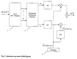
- FIG. 1 shows schematically the processing of an MQAM signal on the transmitter side.
- several m bits of the serial data stream to be transmitted are combined in a series / parallel converter 1 to form a complex complex symbol of higher value.
- the complex symbol space comprises M elements.
- complex symbol words with a real part and an imaginary part are generated in the mapper 2, which are then combined to form the MQAM high-frequency signal to be transmitted by the carrier frequencies of a carrier generator 3 that are phase-shifted by 90 ° with respect to one another.
- Fig. 2 shows the associated quadrature receiver.
- the received MQAM high-frequency signal is again mixed down into the baseband in two mixers 4 and 5 with the superimposition frequencies of a carrier oscillator 6, which are phase-shifted by 90 ° relative to one another, and then the baseband signals are generated by means of a clock generator 7, the clock frequency of which corresponds to the clock frequency specific to the MQAM method used, scanned.
- the sampling rate must be chosen so large that the sampling theorem is fulfilled.
- the oscillator 6 is no longer readjusted to the exact carrier frequency and carrier phase value, but the frequency of the oscillator 6 is set to the transmitter-side carrier frequency only to a few percent of the symbol rate.
- the phase of the clock generator 7 is also not regulated, only the clock frequency is set to the value of the MQAM method used.
- the clock phase error still present is compensated for by a subsequent arithmetic operation, as is the frequency and phase error of the carrier possibly existing by the non-controlled oscillator 6. This compensation of the baseband signals takes place in a compensation arrangement 8, the function and mode of operation of which is described in more detail below.
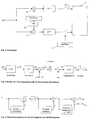
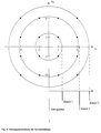
- FIG 3 shows the transmission model described with reference to FIGS. 1 and 2 in the equivalent baseband representation.
- the starting point is the digital complex symbol sequence s 0 (t) to be transmitted.
- the time offset ⁇ T s unknown in the receiver compared to the ideal sampling times is realized by the following system block.
- the values ⁇ are in the range -0.5 ⁇ ⁇ ⁇ 0.5
- AWGN additive white Gaussian noise
- n ( t ) n I. ( t ) + jn Q (t ) complex.
- the real part n I ( t ) and the imaginary part n Q ( t ) have the bilateral power density spectrum (LDS) N 0/2 and are statistically independent of each other.
- LDS bilateral power density spectrum
- 2nd ⁇ ⁇ 1 T s 0 T s E ⁇
- 2nd ⁇ ⁇ ⁇ T s 0 T s E ⁇
- the sequence x ⁇ (see also FIG. 1) is first used to estimate the clock phase from the unknown standardized time offset ⁇ .
- the process for clock synchronization is feedback-free and known (K. Schmidt: Digital clock recovery for bandwidth-efficient mobile radio systems, thesis, Inst. For communications technology, Darmstadt, Dec. 1993 and Oerder: Algorithms for digital clock synchronization for data transmission, Chair of Electrical Control, Aachen, 1989) .
- the estimated time shift ⁇ ⁇ T s (the roof is generally used for estimates) can be undone by an interpolation filter.
- Sub-sampling is then carried out by the oversampling factor o ⁇ , so that the sequence w ⁇ represents the phase-shifted samples at the symbol times.
- the dynamic estimation of the unknown coefficients c (see FIG. 1) is then carried out and with the estimated value c ⁇ the multiplication undone.
- the resulting sequence z ⁇ is then used for frequency and phase estimation.
- the sequence w ⁇ arises, which in the ideal case is equal to the transmitted symbol sequence a ⁇ .
- Basic considerations on compensation can be found in (K. Schmidt: “Digital Clock Recovery for Bandwidth-Efficient Mobile Radio Systems", Dissertation, Inst. For Communication Technology, Darmstadt, Dec. 1993 and Kammeyer: “News Transmission”, Teubner-Verlag, Stuttgart, 1992).
- a first estimation of the dynamics is carried out by comparing the average useful signal amount with the ideal expected value of the symbol amount of a corresponding MQAM constellation.
- the estimated value of the first stage thus gives the predicted value according to Eq . ( 1 )
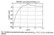
- the method of rough estimation is developed based on the maximum likelihood theory.
- the principle of dynamic estimation is based on the correlation of the relative frequency of the symbol amounts read in with the distribution density function of an ideal MQAM signal.
- the starting point is the following approach for the maximum likelihood function. A limited number of symbols is assumed with an unlimited observation period. The expected value should be maximized over the entire observation sequence.
- the product can be designed according to the expected value formation.
- log likelihood function After logarithmization, the so-called log likelihood function is obtained. This offers the advantage that no products have to be formed, but rather sums. This simpler implementation is permissible since the In function increases in a strictly monotonous manner and the position of the maximum is not changed.
- This non-linearity is shown by way of example in FIG. 6 .
- the aim now is to simplify the nonlinearity NL (
- T s N 0 T s ⁇
- 2nd ⁇ E s N 0 ⁇ 1
- the signal-to-noise ratio represents a freely selectable constant in these considerations, it is assumed in the following that the signal-to-noise ratio E s / N is 0 >> 1 and thus in the region of the maximum
- n ⁇ indicates how often the amount
- c ⁇ is now varied over a range that must cover the maximum error of the prediction.
- the step size dc must be chosen so fine in accordance with the modulation method so that as far as possible no wrong amount decisions of the â ⁇
- factor c ⁇ 2 is selected, which maximizes the log likelihood function Eq. (4). This corresponds to the correlation of the histogram of the received symbol amounts with that of an ideal constellation in FIG. 8 . This is the rough estimate c ⁇ 2 before.
- the fine estimation works data-aided, ie after compensation with the previously estimated c ⁇ 2 first the symbol amounts
- are from the previous rough estimate for the dynamic estimate c ⁇ 2 used.
- the carrier and phase synchronization is carried out according to the NDA method ( N on- D ata- A ided, ie without knowledge of the transmitted symbols a ⁇ ) based on the maximum likelihood theory.
- the following DA procedure DA procedure ( D ata- A ided, ie with the help of estimated symbols â ⁇ ) is optional and achieves the theoretically possible error variance of the estimated frequency and phase. This procedure only has to be used if maximum accuracy chain (eg with a small number of symbols N ) is required.
- the algorithm delivers estimates ⁇ f ⁇ for the frequency offset and ⁇ ⁇ ⁇ for the phase shift.
- the algorithm presented here is implemented in an open - open loop Structure implemented analytically.
- the expression E a ⁇ ⁇ describes the expected value with respect to the N symbols a ⁇ transmitted.
- the values of the test parameters (generally marked with a snake) ⁇ f ⁇ and ⁇ , at which the likelihood function becomes maximum, are estimated.
- MQAM transmission M equally probable symbols A ⁇ occur.
- the likelihood function can be used simplify const with the constant of no further interest. It can be seen that in the likelihood function there are no longer any analog time profiles, but only the scanning sequence z ⁇ (see FIG. 3) at the symbol times.
- the loganthmus function increases monotonously and does not change the maximum.
- the log-likelihood function according to Eq. (6) is obtained.
- NL ( z ) Fourier series development of NL ( z ) is carried out with regard to the phase.
- e.g.
- ⁇ e j ⁇ the nonlinearity can be determined by the Fourier series according to Eq. (9)
- phase ⁇ ( ⁇ ) in Eq. (17) due to the 2 ⁇ periotic nature of the cos function, 2 ⁇ jumps may still occur, while in the approximation in Eq. (18) these 2 ⁇ jumps no longer occur may, which is why unwrapped phase ⁇ u ( ⁇ ) is defined in the approximation. This situation is illustrated in FIG. 12 .
- the estimate uses generalized N sum values, which will be discussed below.
- the frequency offset searched results from the calculation of a linear, amount-weighted regression.
- the cyclic folding of the FFT corresponds to the linear folding of the z-transformation if the following applies to the FFT length:
- phase difference ⁇ ( ⁇ ) ⁇ [- ⁇ , + ⁇ ] of two successive terms is first determined, these difference values are then added up.
- the block diagram for calculating the continuous phase is shown in FIG. 12 .
- the problem arises that data-dependent errors can lead to a drop in the amount in sum ( ⁇ ), which can lead to the occurrence of undesired 2 ⁇ jumps in the calculation of the continuous phase profile ⁇ U ( ⁇ ) cycle slips .
- the linear regression and the estimated value ⁇ determined from it f ⁇ are thus unusable, as illustrated in FIG. 13 . If there is a drop in the amount, 2 ⁇ jumps can occur in the determined, continuous phase profile.
- the estimated phase curve then deviates significantly from the ideal phase curve.
- phase offset can thus be calculated by forming an argument according to Eq. (23) :
- cycle slips (2 ⁇ phase jumps in the calculation of the continuous unwrapped phase) had to be solved for the phase regression, which occur due to a drop in the amount of the complex pointer.
- These cycle slips are efficiently suppressed by multiple folding operations, ie the amount fluctuations are significantly reduced with each folding. As far as I know, this folding process to avoid cycle slips is also new.
- the result of the weighted phase regression is then the estimate of the frequency offset.
- the received signal is compensated with the estimated frequency offset and the output data set is used to estimate the phase offset.
- the estimation of the phase offset again using the first Fourier coefficient of the likelihood function. Subsequently, an improved DA estimate can optionally be carried out.
- the estimated symbol sequence must be available. For this need of FIG. 19 from the first frequency- and phase-compensated sequence w ⁇ the symbols â ⁇ are estimated by a threshold value. The remaining fine estimates ⁇ f fine and ⁇ fine become by maximizing the log-likelihood function
- FIG. 19 The block diagram of the DA method is shown in FIG. 19.
Landscapes
- Engineering & Computer Science (AREA)
- Computer Networks & Wireless Communication (AREA)
- Signal Processing (AREA)
- Digital Transmission Methods That Use Modulated Carrier Waves (AREA)
- Synchronisation In Digital Transmission Systems (AREA)
Abstract
Description
Die Erfindung betrifft eine Verfahren laut Oberbegriff des Hauptanspruches.The invention relates to a method according to the preamble of the main claim.
Zur Demodulation von höherstufigen QAM (Quadratur Amplituden Moduliert)-Signalen (z.B. 4-,16-, 32-, 64-, 128-, 256-QAM-Signale) werden empfangsseitig die empfangenen Hochfrequenzsignale mit einem Oszillator, dessen Überlagerungsfrequenz der senderseitigen Träger-Frequenz entspricht, ins Basisband umgesetzt. Diese Basisbandsignale werden dann mit einer Taktfrequenz, die durch das angewendete QAM-Modulationsverfahren vorbestimmt ist, abgetastet. Die bisher bekannten Demodulationsverfahren für solche MQAM-Signale arbeiten mit Regelschaltungen, durch die die Frequenz und Phase des Überlagerungsoszillators exakt auf die Frequenz und Phase des senderseitigen Trägers geregelt wird (DE 43 06 881, 44 10 607 bzw. 44 46 637). Aus den so mittels eines geregelten Oszillators ins Basisband umgesetzten Basisbandsignalen wird dann über einen Phasendetektor ein phasenrichtiges Taktsignal abgeleitet, mit dem dann die Basisbandsignale jeweils exakt zu den vorbestimmten Symbolzeitpunkten abgetastet werden (beispielsweise nach Hoffmann, "A new carrier regeneration scheme for QAM signals", IEEE International Symposium on Circuits and Systems, Finland, June 88, pp. 599-602).For the demodulation of higher-level QAM ( Q uadratur A mplituden M modulated) signals (e.g. 4-, 16-, 32-, 64-, 128-, 256-QAM signals), the received high-frequency signals are received on the receiving side with an oscillator, the beat frequency of which Carrier frequency on the transmitter side, converted to baseband. These baseband signals are then sampled at a clock frequency which is predetermined by the QAM modulation method used. The previously known demodulation methods for such MQAM signals work with control circuits by means of which the frequency and phase of the local oscillator are regulated exactly to the frequency and phase of the transmitter-side carrier (DE 43 06 881, 44 10 607 and 44 46 637). A phase-corrected clock signal is then derived from the baseband signals thus converted into the baseband by means of a controlled oscillator, with which the baseband signals are then sampled exactly at the predetermined symbol times (for example, according to Hoffmann, "A new carrier regeneration scheme for QAM signals", IEEE International Symposium on Circuits and Systems, Finland, June 88, pp. 599-602).
Diese bekannten Demodulationsverfahren besitzen den Nachteil einer relativ langen Akquisitionszeit, die im Extremfall zu einem sogenannten Hangup führen kann. Sie sind nur für sehr lange Symbolfolgen einsetzbar, bei denen die Akquisitionszeit eine untergeordnete Rolle spielt. Für sogenannte TDMA-Übertragungen (Time Division Multiple Access) mit sehr kurzen Symbolfolgen sind diese bekannten Verfahren nicht geeignet.These known demodulation methods have the disadvantage of a relatively long acquisition time, which in extreme cases can lead to a so-called hangup. They can only be used for very long symbol sequences in which the acquisition time plays a subordinate role. For so-called TDMA transmissions (Time Division Multiple Access) with very short symbol sequences, these known methods are not suitable.
Es ist daher Aufgabe der Erfindung, ein Demodulationsverfahren für solche MQAM-Signale zu schaffen, mit dem auch ohne Kenntnis der übertragenen Symbole auch für kurze Symbolfolgen eine schnelle Synchronisation durchführbar ist.It is therefore an object of the invention to provide a demodulation method for such MQAM signals, with which rapid synchronization can be carried out even for short symbol sequences even without knowledge of the symbols transmitted.
Diese Aufgabe wird gelöst durch ein Verfahren laut Hauptan spruch, vorteilhafte Weiterbildungen ergeben sich aus den Unteransprüchen.This object is achieved by a method according to the main claim, advantageous further developments result from the subclaims.
Ein erfindungsgemäßes Verfahren ermöglicht rein analytisch ohne Regelung eine schnelle Synchronisation der empfangenen QAM-Signale. Damit ist die Akquisitionszeit exakt definiert und es können keine sogenannten Hangups auftreten. Außerdem ist keine Kenntnis der Übertragenen Symbole notwendig. Die Synchronisationsparameter wie Takt, Phase, Trägerfrequenz- und Trägerphasenversatz werden beim erfindungsgemäßen Verfahren rein analytisch berechnet und zwar mit einem sehr geringen Rechenaufwand. Ein grundsätzlicher Unterschied gegenüber den bekannten Demodulationsverfahren besteht darin, daß der Überlagerungsoszillator zur Rückumsetzung ins Basisband nicht mehr bezüglich Frequenz und Phase auf den Sollwert geregelt wird, sondern daß nur ein auf einige Prozent der Symbolrate genau auf die Trägerfrequenz eingestellter Überlagerungsoszillator verwendet wird, während ein eventueller Frequenz- und Phasenfehler rein rechnerisch durch entsprechende Kompensation der Basisbandsignale berücksichtigt wird. Gleiches gilt für den freilaufenden Taktgenerator, dessen Taktfrequenz ist entsprechend dem angewendeten MQAM-Verfahren gewählt und ein eventueller Taktphasenfehler wird nicht ausgeregelt, sondern wiederum durch entsprechende Kompensation der Basisbandsignale eliminiert. Selbst bei einer 256-QAM-Modulation ist eine Synchronisation in kürzester Zeit in einem Beobachtungsintervall von nur 200 Symbolperioden möglich. Ein erfindungsgemäßes Verfahren eignet sich daher besonders für die Demodulation von TDMA-Übertragungsverfahren mit nur kurzen Symbolfolgen innerhalb eines Bursts.A method according to the invention enables fast synchronization of the received QAM signals purely analytically without regulation. This means that the acquisition time is precisely defined and no so-called hangups can occur. In addition, no knowledge of the transmitted symbols is necessary. The synchronization parameters such as clock, phase, carrier frequency and carrier phase offset are calculated purely analytically in the method according to the invention, and indeed with very little computing effort. A fundamental difference compared to the known demodulation methods is that the local oscillator for converting back to baseband is no longer controlled in terms of frequency and phase to the setpoint, but that only a local oscillator set to a few percent of the symbol rate is used, while a possible one Frequency and Phase error is taken into account purely arithmetically by appropriate compensation of the baseband signals. The same applies to the free-running clock generator, whose clock frequency is selected in accordance with the MQAM method used, and any clock phase error is not corrected, but is instead eliminated by appropriate compensation of the baseband signals. Even with 256-QAM modulation, synchronization is possible in the shortest possible time in an observation interval of only 200 symbol periods. A method according to the invention is therefore particularly suitable for the demodulation of TDMA transmission methods with only short symbol sequences within a burst.
Das zur Abschätzung des Frequenz- und Phasenversatzes vorgeschlagene erfindungsgemäße Berechnungsverfahren nach Anspruch 5 für den Träger ist nicht nur für diesen Zweck geeignet, sondern konnte auch für andere Zwecke eingesetzt werden, beispielsweise zum Abschätzen der Frequenz eines gestörten Sinussignales unbekannter Frequenz.The calculation method according to the invention for the carrier, which is proposed for estimating the frequency and phase offset, is not only suitable for this purpose, but could also be used for other purposes, for example for estimating the frequency of a disturbed sinusoidal signal of unknown frequency.
Die Erfindung wird im folgenden anhand schematischer Zeichnungen an Ausführungsbeispielen näher erläutert.The invention is explained below with reference to schematic drawings of exemplary embodiments.
Fig. 1 zeigt schematisch die senderseitige Aufbereitung eines MQAM-Signals. Hierbei werden in einem Serien/Parallel-Wandler 1 mehrere m-Bit des zu übertragenden seriellen Datenstromes zu einem höherwertigen komplexen Symbol zusammengefaßt. Der komplexe Symbolraum umfaßt M Elemente. In dem Mapper 2 werden auf diese Weise komplexe Symbolworte mit Realteil und Imaginärteil erzeugt, die anschließend durch die um 90° gegeneinander phasenverschobenen Trägerfrequenzen eines Tragergenerators 3 zu dem auszusendenden MQAM-Hochfrequenzsignal vereint werden.1 shows schematically the processing of an MQAM signal on the transmitter side. In this case, several m bits of the serial data stream to be transmitted are combined in a series /
Fig. 2 zeigt den zugehörigen Quadraturempfänger.Fig. 2 shows the associated quadrature receiver.
Das empfangene MQAM-Hochfrequenzsignal wird wieder in zwei Mischern 4 und 5 mit den um 90° gegeneinander phasenverschobenen Überlagerungsfrequenzen eines Trägeroszillators 6 ins Basisband herabgemischt und anschließend werden die Basisbandsignale mittels eines Taktgenerators 7, dessen Taktfrequenz der dem jeweils angewendeten MQAM-Verfahren eigenen Taktfrequenz entspricht, abgetastet. Die Abtastrate muß so groß gewählt werden, dass das Abtasttheorem erfüllt ist.The received MQAM high-frequency signal is again mixed down into the baseband in two
Im Gegensatz zu bekannten Demodulationsverfahren wird gemäß der Erfindung der Oszillator 6 nicht mehr auf den exakten Trägerfrequenz und Trägerphasenwert nachgeregelt, sondern der Oszillator 6 ist in seiner Frequenz nur auf einige Prozent der Symbolrate genau auf die senderseitige Trägerfrequenz eingestellt. Auch der Taktgenerator 7 wird nicht in seiner Phase geregelt, nur die Taktfrequenz ist auf den Wert des angewendeten MQAM-Verfahrens eingestellt. Gemäß der Erfindung wird durch einen anschließenden Rechenvorgang der noch bestehende Taktphasenfehler kompensiert, ebenso der durch den nicht geregelten Oszillator 6 eventuell bestehende Frequenz- und Phasenfehler des Trägers. Diese Kompensation der Basisbandsignale erfolgt in einer Kompensationsanordnung 8, deren Funktion und Wirkungsweise nachfolgend näher beschrieben wird.In contrast to known demodulation methods, according to the invention, the
Fig. 3 zeigt das anhand der Fig. 1 und 2 geschilderte Übertragungsmodell in der äquivalenten Basisbanddarstellung.3 shows the transmission model described with reference to FIGS. 1 and 2 in the equivalent baseband representation.
Ausgangspunkt ist die zu übertragende digitale komplexe Symbolfolge s 0 (t) ![]()
![]()
Dieses Signal läßt sich darstellen als die Summe zweier mit den Symbolwerten a I ,ν , a Q ,ν gewichteter Diracimpulse zu den Zeiten ![]()
![]()
![]()
![]()
![]()
![]()
Der im Empfänger unbekannte Zeitversatz ε T s gegenüber den idealen Abtastzeitpunkten wird durch den nachfolgenden Systemblock realisiert. Die Werte ε liegen dabei in dem Bereich![]()
![]()
Für s(t) erhält man![]()
![]()
Der auftretende Frequenzversatz Δf und Phasenversatz ΔΦ bei der Demodulation werden durch eine Multiplikation mit dem Drehzeiger e j(2πΔft+ΔΦ) berücksichtigt.
Das Sendesignal s M (t) im äquivalenten Basisband ergibt sich auf diese Weise zu![]()
The transmission signal s M ( t ) in the equivalent baseband results in this way ![]()
Das Sendesignal s M (t) wird auf der Übertragungsstrecke durch additives weißes Gaußsches Rauschen (AWGN) n(t) gestört, es entsteht das Empfangssignal r(t)![]()
![]()
Im Falle der betrachteten QAM-Übertragung ist das Rauschen ![]()
![]()
![]()
![]()
![]()
![]()
Die in Fig. 1 dargestellte Ausgangsfolge x ν liegt mit einem Oversampling-Faktor von ![]()
![]()
Die Synchronisation gliedert sich nach Fig. 4 in drei Stufen :
- A. Taktsynchronisation
- B. Dynamikschätzung
- C. Trägersynchronisation
- A. Clock synchronization
- B. Dynamic Estimation
- C. Carrier synchronization
Die Folge x ν (siehe auch Fig. 1) wird zuerst zur Taktphasenschätzung von dem unbekannten normierten Zeitversatz ε verwendet. Das Verfahren zur Taktsynchronisation ist rückkopplungsfrei und bekannt (K. Schmidt: Digitale Taktrückgewinnung für bandbreiteneffiziente Mobilfunksysteme, Dissertation, Inst. für Nachrichtentechnik, Darmstadt, Dez. 1993 und Oerder: Algorithmen zur digitalen Taktsynchronisation bei Datenübertragung, Lehrstuhl für Elektrische Regelungstechnik, Aachen, 1989). Anschließend wird die geschätzte zeitliche Verschiebung ![]()
![]()
![]()
![]()
Bei allen Schätzungen wird ein Beobachtungsintervall von N Symbolperioden vorausgesetzt.An observation interval of N symbol periods is assumed for all estimates.
Die Dynamikschätzung ist notwendig, weil bei einer MQAM-Übertragung sowohl in der Symbolphase als auch im Symbolbetrag eine Information enthalten ist. Die Dynamikschätzung wird in bis zu drei Stufen durchgeführt:
- 1. Vorschätzung: Zuerst wird eine erste grobe Schätzung der Dynamik analytisch durch Vergleich des berechneten Mittelwertes des Nutzsignalbetrages mit dem statistischen Mittelwert des Symbolbetrages der entsprechenden MQAM-Modulation durchgeführt.
- 2. Grobschätzung: Anschließend wird durch ein Suchverfahren die zu schätzende multiplikative Konstante variiert und diejenige Konstante ausgewählt, welche die Log-Likelihood-Funktion maximiert. Dieses Verfahren zur Dynamikschätzung kann auch als Korrelation der Verteilungsdichtefunktion der empfangenen Symbolbeträge mit der statischen Verteilungsdichtefunktion der Symbolbeträge interpretiert werden.
- 3. Feinschätzung: Ausgehend von diesem Wert wird anschließend der Feinschätzungwert analytisch in Anlehnung an die Maximum-Likelihood-Theorie berechnet.
- 1. Estimation: First, a first rough estimate of the dynamics is carried out analytically by comparing the calculated mean value of the useful signal amount with the statistical mean value of the symbol amount of the corresponding MQAM modulation.
- 2. Rough estimate: The search method then uses a search method to vary the multiplicative constant to be estimated and to select the constant that has the log likelihood function maximized. This method for dynamic estimation can also be interpreted as a correlation of the distribution density function of the received symbol amounts with the static distribution density function of the symbol amounts.
- 3. Fine estimation: Based on this value, the fine estimation value is then calculated analytically based on the maximum likelihood theory.
Die Anzahl der verwenden Stufen hängt von der gewünschten Genauigkeit ab. Bei großer Beobachtungslänge N reicht z.B. nur die Vorschschätzung aus, während bei kurzer Beoachtungslänge und hoher Stufenzahl M = 256 alle drei Stufen erforderlich sind.The number of levels used depends on the desired accuracy. With a long observation length N, for example, only the forecast is sufficient, while with a short observation length and a high number of stages M = 256 all three stages are required.
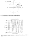
Zunächst wird eine erste Schätzung der Dynamik durch Vergleich des mittleren Nutzsignalbetrages mit dem idealen Erwartungswert des Symbolbetrages einer entsprechenden MQAM-Konstellation durchgeführt. Mit den M verschiedenen Symbolen A α eines MQAM-Symbolalphabetes berechnet sich der ideale Erwartungswert Betr id der Symbolbeträge zu:![]()
![]()
Im einzelnen ergeben sich für die unterschiedlichen Modulationsstufen folgende Werte:

Der geschätzte Betrag ergibt sich aus den N Werten durch![]()
![]()
Der Schätzwert der ersten Stufe ergibt damit der Vorschätzwert nach Gl.(1)
Das Verfahren der Grobschätzung wird in Anlehnung an die Maximum-Likelihood-Theorie entwickelt. Das Prinzip der Dynamikschätzung beruht auf der Korrelation der relativen Häufigkeit der eingelesenen Symbolbeträge mit der Verteilungsdichtefunktion eines idealen MQAM-Signales.
Ausgangspunkt ist der folgende Ansatz für die Maximum-Likelihood-Funktion. Angenommen wird eine begrenzte Symbolzahl bei einer unbegrenzten Beobachtungsdauer. Es soll der Erwartungswert über die gesamte Beobachtungssequenz maximiert werden.
The starting point is the following approach for the maximum likelihood function. A limited number of symbols is assumed with an unlimited observation period. The expected value should be maximized over the entire observation sequence.
Da der Schätzparameter nicht enthalten ist, darf man r(t) weglassen und dafür mit T s ·|x ν|2 erweitern. Mit der Normierung![]()


![]()
Nun kann der Exponent zusammengefaßt werden und man erhält
Da die Einzelsymbole a ν voneinander statistisch unabhängig sind, kann die ProduktFig.ung nach der Erwartungswertbildung ausgeführt werden.
Die Werte Δf, ΔΦ sind nicht bekannt und sollen aus Aufwandsgründen nicht als Versuchsparameter eingesetzt werden. Da das Maximum der Log-Likelihood-Funktion gesucht wird, ist nach Fig. 5 bei hinreichend großem Störabstand die Abweichung![]()
![]()
![]()
![]()
Diese Näherung ist notwendig, weil e νt wegen des unbekannten Frequenz- und Phasenversatzes ebenfalls nicht bekannt ist.This approximation is necessary because e νt is also unknown due to the unknown frequency and phase offset.
Durch diese Approximation entsteht kein datenabhängiger Schätzfehler, da bei einem steigenden Störabstand E s /N 0 → ∞ die Folge![]()
![]()
![]()
![]()
![]()
![]()
Durch Einstzen von Gl.(3) in die Log-Likelihood-Funktion ergibt sich
Nach Logarithmieren erhält man die sogenannte Log-Likelihood-Funktion. Das bietet den Vorteil, daß keine Produkte gebildet werden müssen, sondern Summen. Diese einfachere Realisierung ist zulässig, da die In-Funktion streng monoton steigend ist und damit die Lage des Maximums nicht verändert wird.
Dieser Ausdruck ist somit nur noch vom Betrag der empfangenen Symbole abhängig, der Frequenz- und Phasenversatz gehen durch die vorgenommenen Näherungen nicht mit ein. Die Erwartungswertbildung über alle M möglichen Symbole des Symbolalphabetes a ν ∈ A α mit den Beträgen |A α| liefert
Diese Nichtlinearität wird für beispielhaft in Fig. 6 gezeigt. Ziel ist es nun, die Nichtlinearität NL(|x ν|,c̃) zu vereinfachen.This non-linearity is shown by way of example in FIG. 6 . The aim now is to simplify the nonlinearity NL (| x ν |, c̃ ).
Zwischen dem Term![]()

![]()
![]()
![]()
Da der Störabstand in diesen Betrachtungen eine frei wählbare Konstante darstellt, geht man im folgenden davon aus, daß der Störabstand E s /N 0 >> 1 ist und damit nach Fig. 5 im Bereich des Maximums |x ν| → c̃|â ν| konvergiert.
In der Näherung gibt n α an, wie oft der Betrag |A α| in der Summe über die M Werte des Symbolalphabetes vorkommt, außerdem wird jedem Symbolbetrag |x ν| ein geschätzter idealer Betrag |c̃|â ν| zugeordnet.
Für die Implementierung der Nichtlinearität werden also die Überlappungen der einzelnen ![]()
![]()

For the implementation of the non-linearity, the overlaps of the individual ![]()
![]()
Zur Approximation der Log-Likelihood-Funktion wird![]()
![]()

![]()
![]()
Man beachte, daß |â ν| für jeden Versuchsparemeter c̃ neu geschätzt werden muß, weil abseits vom zu schätztenden c viele Entscheidungsfehler gemacht werden. Ein simuliertes Beispiel wird in Fig. 7 für eine 256QAM mit einem zu schätzenden c = 1 gezeigt.Note that | â ν | for each experimental parameter c̃ has to be re-estimated, because apart from the c to be estimated, many decision errors are made. A simulated example is shown in Fig. 7 for a 256QAM with a c = 1 to be estimated.
In einer Schleife wird nun c̃ über einen Bereich variiert, der den maximalen Fehler der Vorschätzung abdecken muß. Dieser Fehler liegt bei durchgeführten Simulationen bei kurzen Beobachtungslängen bei maximal 10%, d.h. nach erfolgter Korrektur mit dem Vorschätzwert ![]()
![]()

![]()
![]()
Es wird derjenige Faktor ![]()
![]()
![]()
![]()
Die Feinschätzung arbeitet data-aided, d.h. nach Kompensation mit dem vorher geschätzten ![]()
![]()
![]()
![]()
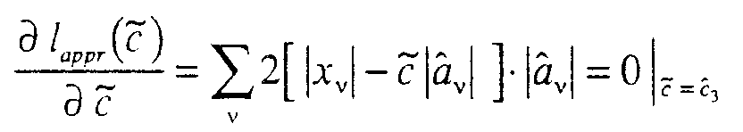
Im Maximum von l appr (c̃) gilt ![]()

![]()
Die Schätzwerte |â ν| werden von der vorhergehenden Grobschätzung beim Dynamikschätzwert ![]()
![]()
Der Ausdruck ist leicht überprüfbar. Unter der Annahme eines unendlich großen Störabstandes ![]()
![]()
![]()
den korrekten Wert. Der Ablauf zur Dynamikkorrektur kann so an die Modulationsstufe, die gewünschte Genauigkeit, die vorliegenden Signalgeräuschleistungsverhältnisse sowie an die verwendete Datensatzlänge adaptiert werden, indem nur die notwendigen Stufen des Schätzverfahrens eingesetzt werden.The printout is easy to check. Assuming an infinitely large signal-to-noise ratio ![]()
![]()
![]()
the correct value. The procedure for dynamic correction can thus be adapted to the modulation level, the desired accuracy, the existing signal-to-noise ratio and the length of the data set used by using only the necessary levels of the estimation method.
Als Maß für die Güte der Dynamikkorrektur wird die Standardabweichung des geschätzten Faktors ![]()
![]()
![]()
![]()
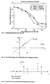
Hierzu wird in Fig. 9 die simulierte Standardabweichung der Dynamikschätzung einer 256QAM (c = 1 eingestellt) für verschiedene Beobachtungslängen (= Anzahl der Symbole N) bei Verwendung aller drei Stufen gezeigt. Gemäß Tabelle auf Seite 11 muß zur fehlerfreien Symbolentscheidung![]()
![]()
Die Träger- und Phasensynchronisation wird nach dem NDA-Verfahren (Non-Data-Aided, d.h. ohne Kenntnis der übertragenen Symbole a ν) durchgeführt in Anlehnung an die Maximum-Likelihood-Theorie durchgeführt. Das nachfolgende DA-Verfahren DA-Verfahren (Data-Aided, d.h. mit Hilfe von geschätzten Symbole â ν) ist optional und erreicht die theoretisch mögliche Fehlervarianz der geschätzten Frequenz und Phase. Dieses Verfahren muß nur dann verwendet werden, wenn maximale Genauigkett (z.B. bei geringer Symbolzahl N) gefordert wird.The carrier and phase synchronization is carried out according to the NDA method ( N on- D ata- A ided, ie without knowledge of the transmitted symbols a ν ) based on the maximum likelihood theory. The following DA procedure DA procedure ( D ata- A ided, ie with the help of estimated symbols â ν ) is optional and achieves the theoretically possible error variance of the estimated frequency and phase. This procedure only has to be used if maximum accuracy chain (eg with a small number of symbols N ) is required.
Der Algorithmus liefert Schätzwerte Δ![]()
![]()
![]()
![]()
![]()
![]()
![]()
![]()
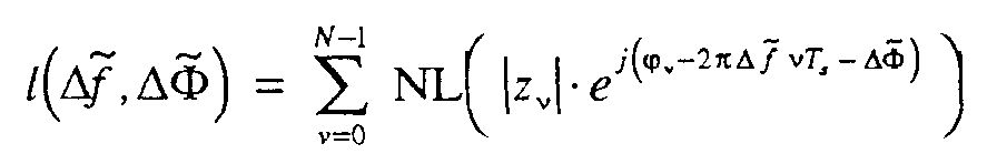
Die zu maximierende Likelihood-Funktion zur Frequenz- und Phasenschätzung lautet (c = 1 und ε = 0 gesetzt)
![]()

![]()
Die Loganthmusfunktion ist monoton steigend und ändert damit das Maximum nicht. Man erhält die Log-Likelihood-Funktion nach Gl.(6) 
Für die nachfolgende Schritte muß gemäß Gl.(7) 

Um zu einem implementierbaren Ansatz zu gelangen, wird folgender verwendet: Es wird eine Fourierreihenentwicklung von NL(z) bezüglich der Phase durchgeführt. Mit Polardarstellung der komplexen Variablen gemäß![]()
![]()
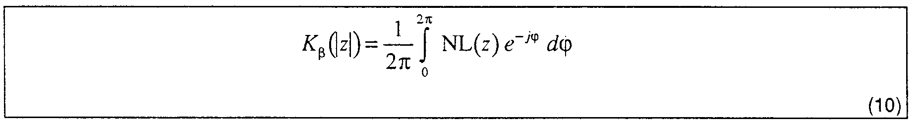
![]()
![]()
- K β(|z|) ist aufgrund der geraden Phasensymmetrie reell K β (| z |) is real due to the even phase symmetry
- wegen der π/2-Phasensymmetrie ist nur jeder vierte Koeffizient β = 0,±4,±8, ··· ungleich Nulldue to the π / 2 phase symmetry, only every fourth coefficient β = 0, ± 4, ± 8, ··· is non-zero
- die Koeffizienten können mit einer FFT berechnet werdenthe coefficients can be calculated with an FFT
-
K β(|z|) werden vorab berechnet und in hinreichend kleinem Δ|z|-Raster in einer Tabelle gelegt. Im Rahmen der Untersuchungen zeigte sich, daß die Koeffizienten K 4(|z|) nur an den idealen Symbolbeträgen

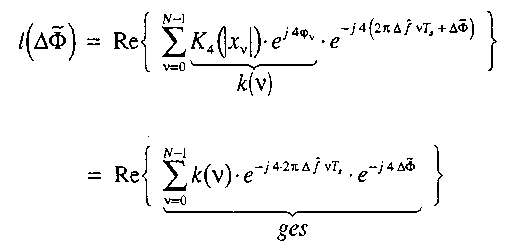
Die Log-Likelihood-Funktion läßt sich somit schreiben:
Der erste Summenausdruck ist für die Fequenz- und Phasenschätzung irrelevant, da dieser unabhängig von den zu schätzenden Parametern ist. In einer ersten Nähetung berücksichtigt man nach Gl.(12) nur den vierte Fourierkoeffizient K 4(|z|):
Im Bereich des Maximums von Gl.(12) gilt näherungsweise Re{···} ≈ |···|, weil der Gesamtzeiger fast exakt auf der positivien Realteilachse liegt. Damit ist die Näherung in Gl.(13) 


![]()

![]()
Der erste Term ist unabhängig von Δf̃ und muß daher nicht berücksichtigt werden. Mit der Polardarstellung nach Gl.(16) 
![]()
![]()
Für die Cosinus-Funktion gilt bei sehr kleinen Argumenten der Näherungsausdruck![]()
![]()
Da das cos-Argument von Gl.(17) im Bereich des Schätzwertes Δ![]()
![]()
![]()
![]()
Man beachte, daß in die Phase β(µ) in Gl.(17) aufgrung der 2π-Periotizität der cos-Funktion noch 2π -Sprünge besitzen darf, während in der Näherung in Gl.(18) diese 2π-Sprünge nicht mehr auftreten dürfen, weshalb auch die ![]()
![]()
![]()
![]()
Anschließend bildet man die erste Ableitung dieses Ausdrucks nach Δf̃, die im Maximum der Log-Likelihood-Funktion (also an der gesuchten Stelle ![]()
![]()
![]()
![]()
Nach Δf̃ aufgelöst erhält man schließlich den analytischen Schätzwert für den Frequenzversatz gemäß Gl.(19) 
Bei der Schätzung werden verallgemeinert N sum Werte verwendet, woraus noch nachfolgend eingegangen wird. Der gesuchte Frequenzversatz ergibt sich also durch die Berechnung einer linearen, betragsgewichteten Regression.The estimate uses generalized N sum values, which will be discussed below. The frequency offset searched results from the calculation of a linear, amount-weighted regression.
Der Summenausdruck sum(µ) von Gl.(15)![]()
![]()
![]()
![]()
Führt man an diesem Ausdruck eine z-Transformation durch, ergibt sich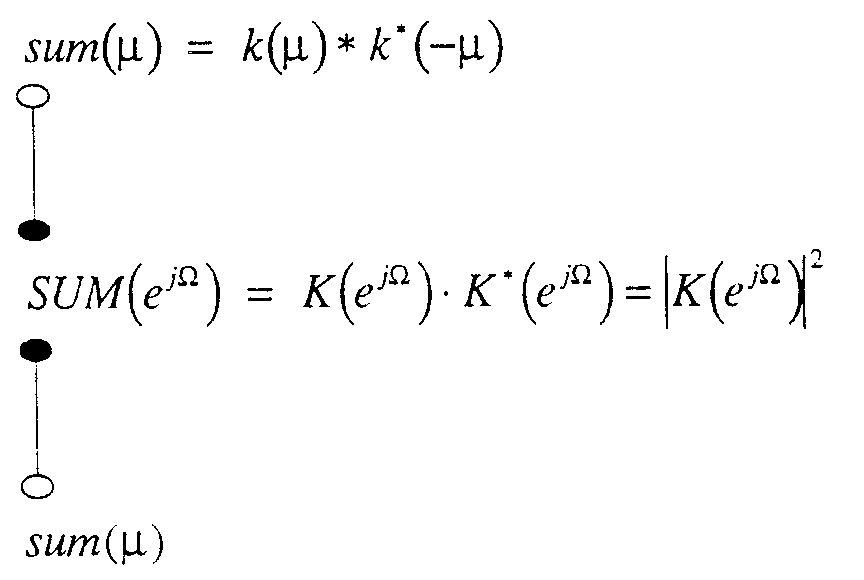
Die zyklische Faltung der FFT entspricht der linearen Faltung der z-Transformation, wenn für die FFT-Länge gilt:![]()
![]()
Dazu werden die entsprechenden Vektoren vor der Transformation mit Nullen aufgefüllt. Der Summenausdruck kann also nach folgendem Vorgehen in Gl.(20) berechnet werden:
Um die ![]()
![]()
![]()
![]()
Bei einer Implementierung ergibt sich das Problem, daß datenabhängige Fehler zu Betragseinbrüchen in sum(µ) führen können, die bei der Berechnung des kontinuierlichen Phasenverlaufes β U (µ) zu einem Auftreten von unerwünschten 2π-Sprüngen führen können, sogenannten ![]()
![]()
![]()
![]()
![]()
![]()
Strategien, cycle slips zu detektieren und anschließend im Phasenverlauf β(µ) die 2π-Sprünge nachträglich zu entfernen, erweißen sich als wenig brauchbar und zu ungenau. Die bessere Lösung ist die Vermeidung der cycle slips. Das wird erreicht, indem die Folge k(ν) in dem Summenausdruck sum(µ) nicht nur einmal, sondern mehrmals mit sich selbst gefaltet wird, was im Frequenzbereich einer erhöhten Potenzierung entspricht und einfach zu berechnen ist. Dadurch tritt ein stärkerer Mittelungseffekt auf und Einbrüche werden vermieden. Die Vorgehensweise von Gl.(20) wird somit durch Gl.(21) erweitert, wobei der Parameter pot den Potenzierungsfaktor angibt.
Die Untersuchungen haben gezeigt, daß pot ≤ 5 selbst bei stark gestörter 256QAM ausreichend ist, höhere Potenzfaktoren bringen keinen werteren Gewinn.The investigations have shown that
Dieses Verfahren zur Unterdrückung von "Cycle Slips" ist meines Wissens noch nicht bekannt und ein Bestandteil des Patentanspruches. Dieses Verfahren zur Vermeidung von "Cycle Slips" ist nicht auf auf die MQAM-Synchronisation beschränkt und sollte globaler patentiert werden. Mit diesem Verfahren kann nämlich die Frequenz Δf einer verallgemeinerten Folge k(ν) gemäß Gl.(22) 
Die Leistungsfägigkeit wird durch Fig. 14,15 demonstriert. In beiden Figuren wird sum(ν) für eine
![]()
![]()
![]()
![]()
Summenwerte (N ist die Beobachtungslänge in Symbolperioden) aus, mehr Summenwerte verbessern das Schätzergebnis nicht mehr. Selbst bei wesentlich kleinerem N sum erhält man sehr ähnliche Fehlervarianzen, bei den Simulationen wurde N sum = 0.25·N verwendet. Sum values ( N is the observation length in symbol periods), more sum values no longer improve the estimation result. Even with a much smaller N sum , very similar error variances are obtained; in the simulations, N sum = 0.25 · N was used.
Nachdem ein Schätzwert Δ![]()
![]()
![]()
![]()
Dieser Ausdruck ist maximal, wenn in der Formel der Gesamtausdruck ges rein reell ist. Damit kann der Phasenversatz über eine Argumentbildung nach Gl.(23) berechnet werden:
Aufgrund der π/2-Rotationssymmetrie des Symbolalphabetes kann natürlich nur ΔΦ mod π/2 bestimmt werden.Due to the π / 2 rotational symmetry of the symbol alphabet, only ΔΦ mod π / 2 can of course be determined.
Zur Beurteilung der Synchronisation werden die Standardabweichungen der Ergebnisse Δ![]()
![]()

![]()
![]()
In den Fig. 16,17 werden die Simulationsergebnisse für verschiedene Beoachtungslängen gezeigt. Man sieht, daß für E s /N 0 >15 dB eine Stagnation durch den datenabhängigen Schätzfehler, weil nach Gl.(12) nur der erste Fourierkoeffizient verwendet wird. Möchte man die theoretisch möglichen gestrichelten Grenzen erreichen, muß noch der im nächsten Kapitel beschriebene DA-Schätzer nachgeschalten werden. 16 , 17 show the simulation results for different observation lengths. It can be seen that for E s / N 0 > 15 dB stagnation due to the data-dependent estimation error, because according to Eq. (12) only the first Fourier coefficient is used. If you want to reach the theoretically possible dashed limits, you have to add the DA estimator described in the next chapter.
Zusammenfassend kann festgehalten werden: Bisher ist noch kein Verfahren bekannt, mit dem bei hochstufiger MQAM-Modulation analytisch ohne Kenntnis der Symbole der Frequenz- und Phasenversatz berechnet werden kann. Der Ablauf wird nochmals in Fig.(18) zusammen gefaßt. Um auf ein numerisch handhabbares Verfahren zu gelangen, wird eine Fourierreihenentwicklung der Nichtlinearität in der Likelihood-Funktion vorgenommen. Es erweist sich als ausreichend, nur einen Fourierkoeffizienten der Reihe zu verwenden. Dadurch wird es mag ich, durch ein Open-loop-Verfahren mit Hilfe -der Phasenregression in zwei Schritten den Frequenz- und anschließend den Phasenversatz zu berechnen. Weiterhin mußte das Problem der sogenannten cycle slips (2π-Phasensprünge bei der Berechnung der kontinuierlichen ungewrappten Phase) für die Phasenregression gelöst werden, welche aufgrund von Betragseinbrüchen des komplexen Zeigers auftreten. Diese cycle slips werden effizient durch mehrfache Faltungsoperation unterdrückt, d.h. die Betragsschwankungen werden mit jeder Faltung deutlich reduziert. Dieses Faltungsverfahren zur Vermeidung von cycle slips ist nach meiner Kenntnis ebenfalls neuartig. Als Ergebnis der betragsgewichteten Phasenregression erhält man anschließend den Schätzwert des Frequenzversatzes. Als nächstes wird das Empfangssignal mit dem geschätzten Frequenzversatz kompensiert und der Ausgangsdatensatz zur Schätzung des Phasenversatzes verwendet. Die Schätzung des Phasenversatzes wieder unter Verwendung des ersten Fourierkoeffizienten der Likelihood-Funktion. Anschließend kann optional eine verbesserte DA-Schätzung durchgeführt werden.In summary, it can be stated: No method is known yet with which high-level MQAM modulation can be used to calculate the frequency and phase shift analytically without knowledge of the symbols. The process is summarized again in Fig. (18) . In order to arrive at a numerically manageable method, a Fourier series development of the non-linearity is carried out in the likelihood function. It turns out to be sufficient to use only one Fourier coefficient of the series. This makes it a pleasure for me to calculate the frequency and then the phase offset using an open-loop method with the help of the phase regression in two steps. Furthermore, the problem of the so-called cycle slips (2π phase jumps in the calculation of the continuous unwrapped phase) had to be solved for the phase regression, which occur due to a drop in the amount of the complex pointer. These cycle slips are efficiently suppressed by multiple folding operations, ie the amount fluctuations are significantly reduced with each folding. As far as I know, this folding process to avoid cycle slips is also new. The result of the weighted phase regression is then the estimate of the frequency offset. Next, the received signal is compensated with the estimated frequency offset and the output data set is used to estimate the phase offset. The estimation of the phase offset again using the first Fourier coefficient of the likelihood function. Subsequently, an improved DA estimate can optionally be carried out.
In der Literatur wurden DA-Verfahren zur Phasenschätzung z.B. für das QPSK-Modulationsverfahren bereits behandelt (F. M. Gardner: Demodulator Reference Recovery Techniques suited for Digital Implementation, ESA Report, 1988). Allerdings wird nur von einer Phasenschätzung und nicht von einer Frequenz- und Phasenschätzung ausgegangen. Das in der Literatur bekannte Verfahren wurde erweitert, so daß eine Frequenz- und Phasenschätzung möglich ist.DA methods for phase estimation, for example for the QPSK modulation method, have already been dealt with in the literature (FM Gardner: Demodulator Reference Recovery Techniques suited for Digital Implementation, ESA Report, 1988). However, only a phase estimate is assumed and not a frequency and phase estimate. The method known in the literature has been expanded so that frequency and phase estimation is possible.
Bei dem DA-Verfahren muß die geschätzte Symbolfolge vorliegen. Hierzu müssen nach Fig. 19 zuerst aus der frequenz- und phasenkompensierten Folge w ν die Symbole â ν durch einen Schwellwertentscheider geschätzt werden. Die noch verbleibende Feinschätzwerte Δf fein und ΔΦ fein werden durch Maximierung der Log-Likelihood-Funktion
Der in Gl.(24) definierte Zeiger
![]()
![]()
Im Bereich des Maximums ist das cos-Argument sehr klein und deshalb die Näherung![]()
![]()
![]()
![]()
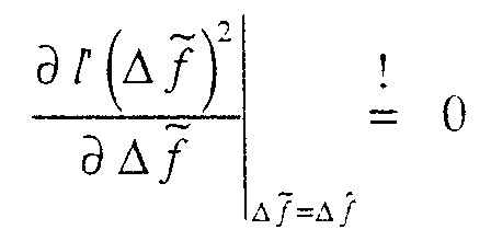
Um das Maximum dieses Ausdruckes zu bestimmen, berechnet man zunächst die partiellen Ableitungen nach Δf̃ fein sowie ΔΦ̃ fein und setzt diese gleich Null:
In matrizieller Form ausgedrückt ergibt sich das Gleichungssystem
Durch Auflösung nach dem Phasen- und Frequenzversatz erhält man die gesuchte Lösung in Gl.(27) 
In Fig. 19 wird das Blockschaltbild des DA-Vefahrens gezeigt.The block diagram of the DA method is shown in FIG. 19.
Claims (6)
Applications Claiming Priority (2)
| Application Number | Priority Date | Filing Date | Title |
|---|---|---|---|
| DE19635444 | 1996-08-31 | ||
| DE19635444A DE19635444C2 (en) | 1996-08-31 | 1996-08-31 | Feedback-free method for demodulating higher-level MQAM signals without knowledge of the symbols transmitted |
Publications (3)
| Publication Number | Publication Date |
|---|---|
| EP0829990A2 true EP0829990A2 (en) | 1998-03-18 |
| EP0829990A3 EP0829990A3 (en) | 2001-09-19 |
| EP0829990B1 EP0829990B1 (en) | 2003-04-09 |
Family
ID=7804326
Family Applications (1)
| Application Number | Title | Priority Date | Filing Date |
|---|---|---|---|
| EP97113420A Expired - Lifetime EP0829990B1 (en) | 1996-08-31 | 1997-08-04 | Method for demodulating high-level M-QAM signals without knowledge of the transmitted symbols |
Country Status (4)
| Country | Link |
|---|---|
| US (1) | US5854570A (en) |
| EP (1) | EP0829990B1 (en) |
| JP (1) | JP3942703B2 (en) |
| DE (2) | DE19635444C2 (en) |
Families Citing this family (16)
| Publication number | Priority date | Publication date | Assignee | Title |
|---|---|---|---|---|
| US6359878B1 (en) | 1998-07-20 | 2002-03-19 | Wirless Facilities, Inc. | Non-data-aided maximum likelihood based feedforward timing synchronization method |
| US6654432B1 (en) | 1998-06-08 | 2003-11-25 | Wireless Facilities, Inc. | Joint maximum likelihood frame and timing estimation for a digital receiver |
| US6430235B1 (en) | 1998-11-05 | 2002-08-06 | Wireless Facilities, Inc. | Non-data-aided feedforward timing synchronization method |
| US6542560B1 (en) * | 1999-04-23 | 2003-04-01 | Lucent Technologies Inc. | Method of channel estimation and compensation based thereon |
| DE19929727C2 (en) * | 1999-06-29 | 2003-01-30 | Siemens Ag | Receiving part for operating a receiving part |
| US6594318B1 (en) * | 1999-12-02 | 2003-07-15 | Qualcomm Incorporated | Method and apparatus for computing soft decision input metrics to a turbo decoder |
| DE10252099B4 (en) * | 2002-11-08 | 2021-08-05 | Rohde & Schwarz GmbH & Co. Kommanditgesellschaft | Measuring device and method for determining a characteristic curve of a high-frequency unit |
| DE60227968D1 (en) * | 2002-12-24 | 2008-09-11 | St Microelectronics Belgium Nv | Fractional time domain interpolator |
| DE102004016937B4 (en) * | 2003-04-07 | 2011-07-28 | Rohde & Schwarz GmbH & Co. KG, 81671 | Method for determining the frequency and / or phase offset in unknown symbols |
| US8204156B2 (en) * | 2008-12-31 | 2012-06-19 | Intel Corporation | Phase error detection with conditional probabilities |
| EP2506516A1 (en) * | 2011-03-31 | 2012-10-03 | Alcatel Lucent | Method of decoding optical data signals |
| FR2996970B1 (en) * | 2012-10-16 | 2015-05-15 | Commissariat Energie Atomique | UWB RECEIVER WITH TEMPORAL DERIVATIVE CORRECTION |
| EP3016339B1 (en) * | 2013-07-15 | 2017-09-13 | Huawei Technologies Co., Ltd. | Cycle slip detection method and device, and receiver |
| GB201322503D0 (en) * | 2013-12-19 | 2014-02-05 | Imagination Tech Ltd | Signal timing |
| CN108761194B (en) * | 2018-03-16 | 2020-06-16 | 贵州电网有限责任公司 | Micropower wireless carrier parameter measuring method based on frequency shift filtering algorithm |
| CN114189417B (en) * | 2021-12-07 | 2023-10-17 | 北京零壹空间电子有限公司 | Carrier frequency synchronization method, carrier frequency synchronization device, computer equipment and storage medium |
Citations (2)
| Publication number | Priority date | Publication date | Assignee | Title |
|---|---|---|---|---|
| DE4101802C1 (en) * | 1991-01-23 | 1992-04-09 | Ant Nachrichtentechnik Gmbh, 7150 Backnang, De | In-phase and quadrature detector for QAM receiver - demodulates using unregulated orthogonal carriers and controls carrier and quadrature phase offsets at baseband |
| EP0579100A1 (en) * | 1992-07-14 | 1994-01-19 | Daimler-Benz Aerospace Aktiengesellschaft | Method and apparatus for baseband phase correction in a PSK receiver |
Family Cites Families (14)
| Publication number | Priority date | Publication date | Assignee | Title |
|---|---|---|---|---|
| DE3531635C2 (en) * | 1985-09-05 | 1994-04-07 | Siemens Ag | Method for two-track digital signal transmission in an asymmetrical band-limited channel using quadrature amplitude modulation |
| DE3700457C1 (en) * | 1987-01-09 | 1988-06-23 | Ant Nachrichtentech | Method and arrangement for synchronizing a receiver in digital transmission systems |
| DE3903944A1 (en) * | 1989-02-10 | 1990-10-11 | Johannes Dr Ing Huber | Symbol clock and carrier phase synchronisation method for coherent digital signal receivers with multi-dimensional signal representation |
| JPH03258147A (en) * | 1990-03-08 | 1991-11-18 | Matsushita Electric Ind Co Ltd | Asynchronous orthogonal demodulator |
| DE4134206C1 (en) * | 1991-10-16 | 1992-12-10 | Ant Nachrichtentechnik Gmbh, 7150 Backnang, De | |
| US5400366A (en) * | 1992-07-09 | 1995-03-21 | Fujitsu Limited | Quasi-synchronous detection and demodulation circuit and frequency discriminator used for the same |
| DE4243787C1 (en) * | 1992-12-23 | 1994-05-26 | Grundig Emv | Method and device for eliminating the frequency offset in received signals of a digital transmission system |
| DE4306881C1 (en) * | 1993-03-05 | 1994-06-16 | Ant Nachrichtentech | QAM receiver with quadrature error correction - uses gradients of detected in=phase and quadrature decision errors |
| DE4410607C1 (en) * | 1994-03-26 | 1995-03-23 | Ant Nachrichtentech | Arrangement for determining the frequency offset in a demodulator for signals with two-dimensional modulation |
| DE4410608C1 (en) * | 1994-03-26 | 1995-03-30 | Ant Nachrichtentech | Arrangement for determining the frequency offset in a demodulator for signals with two-dimensional modulation |
| DE4441566A1 (en) * | 1994-11-23 | 1996-05-30 | Bosch Gmbh Robert | Method for digital frequency correction in multi-carrier transmission methods |
| DE4446637B4 (en) * | 1994-12-24 | 2004-06-03 | Rohde & Schwarz Gmbh & Co. Kg | Arrangement for carrier tracking in an IQ demodulator |
| DE4446639B4 (en) * | 1994-12-24 | 2004-04-29 | Rohde & Schwarz Gmbh & Co. Kg | Method for obtaining an estimate of the carrier frequency and carrier phase of a radio signal modulated according to a coherent multi-stage modulation method for its demodulation in a receiver |
| DE4446640B4 (en) * | 1994-12-24 | 2004-04-29 | Rohde & Schwarz Gmbh & Co. Kg | Arrangement for carrier tracking in an IQ demodulator |
-
1996
- 1996-08-31 DE DE19635444A patent/DE19635444C2/en not_active Expired - Fee Related
-
1997
- 1997-08-04 EP EP97113420A patent/EP0829990B1/en not_active Expired - Lifetime
- 1997-08-04 DE DE59709759T patent/DE59709759D1/en not_active Expired - Lifetime
- 1997-08-26 US US08/918,958 patent/US5854570A/en not_active Expired - Lifetime
- 1997-08-29 JP JP27323297A patent/JP3942703B2/en not_active Expired - Lifetime
Patent Citations (2)
| Publication number | Priority date | Publication date | Assignee | Title |
|---|---|---|---|---|
| DE4101802C1 (en) * | 1991-01-23 | 1992-04-09 | Ant Nachrichtentechnik Gmbh, 7150 Backnang, De | In-phase and quadrature detector for QAM receiver - demodulates using unregulated orthogonal carriers and controls carrier and quadrature phase offsets at baseband |
| EP0579100A1 (en) * | 1992-07-14 | 1994-01-19 | Daimler-Benz Aerospace Aktiengesellschaft | Method and apparatus for baseband phase correction in a PSK receiver |
Non-Patent Citations (1)
| Title |
|---|
| EFSTATHIOU D ET AL: "A COMPARISON STUDY OF THE ESTIMATION PERIOD OF CARRIER PHASE AND AMPLITUDE GAIN ERROR FOR 16-ARY QAM RAYLEIGH FADED BURST TRANSMISSIONS" PROCEEDINGS OF THE GLOBAL TELECOMMUNICATIONS CONFERENCE (GLOBECOM),US,NEW YORK, IEEE, 28. November 1994 (1994-11-28), Seiten 1904-1908, XP000488851 ISBN: 0-7803-1821-8 * |
Also Published As
| Publication number | Publication date |
|---|---|
| DE19635444A1 (en) | 1998-03-12 |
| JP3942703B2 (en) | 2007-07-11 |
| DE59709759D1 (en) | 2003-05-15 |
| EP0829990A3 (en) | 2001-09-19 |
| DE19635444C2 (en) | 1998-06-18 |
| EP0829990B1 (en) | 2003-04-09 |
| US5854570A (en) | 1998-12-29 |
| JPH10173721A (en) | 1998-06-26 |
Similar Documents
| Publication | Publication Date | Title |
|---|---|---|
| DE69818933T2 (en) | Correction of phase and / or frequency shifts in multi-carrier signals | |
| DE69807945T2 (en) | METHOD AND DEVICE FOR FINE FREQUENCY SYNCHRONIZATION IN MULTI-CARRIER DEMODULATION SYSTEMS | |
| EP0829990B1 (en) | Method for demodulating high-level M-QAM signals without knowledge of the transmitted symbols | |
| DE2700354C2 (en) | Receivers for communication systems | |
| DE2735945C2 (en) | Circuit arrangement for the carrier synchronization of coherent phase demodulators | |
| DE69821870T2 (en) | Estimation of the gross frequency offset in multi-carrier receivers | |
| DE69422350T2 (en) | Process for phase recovery and alignment for MSK signals | |
| DE2627446C2 (en) | Arrangement for compensating the carrier phase error in a receiver for discrete data values | |
| DE602004002129T2 (en) | Device for compensating the frequency shift in a receiver, and method therefor | |
| DE19718932A1 (en) | Digital radio receiver | |
| DE69736659T2 (en) | Multi-carrier receiver with compensation for frequency shifts and frequency-dependent distortions | |
| DE69803230T2 (en) | ECHOPHASE DEVIATION COMPENSATION IN A MULTI-CARRIER DEMODULATION SYSTEM | |
| EP1320968B1 (en) | Automatic frequency correction for mobile radio receivers | |
| DE60310931T2 (en) | Pilot supported carrier synchronization scheme | |
| DE19705055A1 (en) | Digital radio receiver and tuning control method | |
| DE69224278T2 (en) | Method for the transmission of reference signals in a multi-carrier data transmission system | |
| DE10303475B3 (en) | Maximum likelihood estimation of the channel coefficients and the DC offset in a digital baseband signal of a radio receiver using the SAGE algorithm | |
| EP0579100B1 (en) | Method and apparatus for baseband phase correction in a PSK receiver | |
| EP0833470B1 (en) | Method for determining the frequency drift of a carrier | |
| EP1537711B1 (en) | Preamble for estimation and equalisation of asymmetries between in phase and quadrature branches in multi-carrier transmission systems | |
| EP1626549B1 (en) | Method and apparatus for estimating carrier frequency using a block-wise coarse estimation | |
| DE19854167C2 (en) | Frequency-stabilized transmission / reception circuit | |
| DE69213496T2 (en) | Method for coherent PSK demodulation and device for its implementation | |
| DE10309262B4 (en) | Method for estimating the frequency and / or the phase of a digital signal sequence | |
| DE69113855T2 (en) | Frequency shift estimation device. |
Legal Events
| Date | Code | Title | Description |
|---|---|---|---|
| PUAI | Public reference made under article 153(3) epc to a published international application that has entered the european phase |
Free format text: ORIGINAL CODE: 0009012 |
|
| AK | Designated contracting states |
Kind code of ref document: A2 Designated state(s): AT BE CH DE DK ES FI FR GB GR IE IT LI LU MC NL PT SE Kind code of ref document: A2 Designated state(s): DE FR GB |
|
| AX | Request for extension of the european patent |
Free format text: AL;LT;LV;RO;SI |
|
| PUAL | Search report despatched |
Free format text: ORIGINAL CODE: 0009013 |
|
| AK | Designated contracting states |
Kind code of ref document: A3 Designated state(s): AT BE CH DE DK ES FI FR GB GR IE IT LI LU MC NL PT SE |
|
| AX | Request for extension of the european patent |
Free format text: AL;LT;LV;RO;SI |
|
| 17P | Request for examination filed |
Effective date: 20011121 |
|
| 17Q | First examination report despatched |
Effective date: 20020129 |
|
| AKX | Designation fees paid |
Free format text: DE FR GB |
|
| GRAH | Despatch of communication of intention to grant a patent |
Free format text: ORIGINAL CODE: EPIDOS IGRA |
|
| GRAH | Despatch of communication of intention to grant a patent |
Free format text: ORIGINAL CODE: EPIDOS IGRA |
|
| GRAA | (expected) grant |
Free format text: ORIGINAL CODE: 0009210 |
|
| AK | Designated contracting states |
Designated state(s): DE FR GB |
|
| REG | Reference to a national code |
Ref country code: GB Ref legal event code: FG4D Free format text: NOT ENGLISH |
|
| GBT | Gb: translation of ep patent filed (gb section 77(6)(a)/1977) |
Effective date: 20030409 |
|
| ET | Fr: translation filed | ||
| PLBE | No opposition filed within time limit |
Free format text: ORIGINAL CODE: 0009261 |
|
| STAA | Information on the status of an ep patent application or granted ep patent |
Free format text: STATUS: NO OPPOSITION FILED WITHIN TIME LIMIT |
|
| 26N | No opposition filed |
Effective date: 20040112 |
|
| REG | Reference to a national code |
Ref country code: FR Ref legal event code: PLFP Year of fee payment: 19 |
|
| REG | Reference to a national code |
Ref country code: FR Ref legal event code: PLFP Year of fee payment: 20 |
|
| PGFP | Annual fee paid to national office [announced via postgrant information from national office to epo] |
Ref country code: GB Payment date: 20160824 Year of fee payment: 20 Ref country code: DE Payment date: 20160829 Year of fee payment: 20 |
|
| PGFP | Annual fee paid to national office [announced via postgrant information from national office to epo] |
Ref country code: FR Payment date: 20160825 Year of fee payment: 20 |
|
| REG | Reference to a national code |
Ref country code: DE Ref legal event code: R071 Ref document number: 59709759 Country of ref document: DE |
|
| REG | Reference to a national code |
Ref country code: GB Ref legal event code: PE20 Expiry date: 20170803 |
|
| PG25 | Lapsed in a contracting state [announced via postgrant information from national office to epo] |
Ref country code: GB Free format text: LAPSE BECAUSE OF EXPIRATION OF PROTECTION Effective date: 20170803 |