EP0706055A2 - Method for calibrating a network analyzer according to the 7-term principle - Google Patents
Method for calibrating a network analyzer according to the 7-term principle Download PDFInfo
- Publication number
- EP0706055A2 EP0706055A2 EP95115297A EP95115297A EP0706055A2 EP 0706055 A2 EP0706055 A2 EP 0706055A2 EP 95115297 A EP95115297 A EP 95115297A EP 95115297 A EP95115297 A EP 95115297A EP 0706055 A2 EP0706055 A2 EP 0706055A2
- Authority
- EP
- European Patent Office
- Prior art keywords
- calibration
- calibration measurement
- port
- measuring
- carried out
- Prior art date
- Legal status (The legal status is an assumption and is not a legal conclusion. Google has not performed a legal analysis and makes no representation as to the accuracy of the status listed.)
- Granted
Links
Images

Classifications
-
- G—PHYSICS
- G01—MEASURING; TESTING
- G01R—MEASURING ELECTRIC VARIABLES; MEASURING MAGNETIC VARIABLES
- G01R27/00—Arrangements for measuring resistance, reactance, impedance, or electric characteristics derived therefrom
- G01R27/28—Measuring attenuation, gain, phase shift or derived characteristics of electric four pole networks, i.e. two-port networks; Measuring transient response
- G01R27/32—Measuring attenuation, gain, phase shift or derived characteristics of electric four pole networks, i.e. two-port networks; Measuring transient response in circuits having distributed constants, e.g. having very long conductors or involving high frequencies
-
- G—PHYSICS
- G01—MEASURING; TESTING
- G01R—MEASURING ELECTRIC VARIABLES; MEASURING MAGNETIC VARIABLES
- G01R35/00—Testing or calibrating of apparatus covered by the other groups of this subclass
-
- G—PHYSICS
- G01—MEASURING; TESTING
- G01R—MEASURING ELECTRIC VARIABLES; MEASURING MAGNETIC VARIABLES
- G01R35/00—Testing or calibrating of apparatus covered by the other groups of this subclass
- G01R35/005—Calibrating; Standards or reference devices, e.g. voltage or resistance standards, "golden" references
Definitions
- the invention is based on a method according to the preamble of the main claim.
- a method of this type is known (DE 39 12 795 or corresponding US Pat. No. 4,982,164).
- This so-called 7-term method has the advantage that only three calibration standards are required.
- a two-port is required for the first calibration measurement, from which all complex scattering parameters are known. This is for object measurements in the coaxial waveguide region most easily by a direct connection of two measuring ports (T hrough measurement) achieved for the second calibration measurement is a reflection-free wave sink (M atch) successively, for example, connected to the two measuring ports, the third calibration measurement is, for example, a one-port reflection known (R eflexion) connected to the two measuring ports in succession (TMR-called calibration).
- L ine For measurements on planar microwave circuits or semiconductor substrates (on-wafer measurements) is the T standard usually not feasible here instead, a well-known line (L ine) will be the first calibration for the first measurement used (LRM calibration for example, described in "Achieving greater on-wafer S-parameter accuracy with the LRM calibration technique" , by A. Davidson, E. Strid and K. Jones, Cascade-Microtech, Product Note).
- This known LRM calibration method which is now used for on-wafer measurements, also requires that all scattering parameters of the electrical line used for the first calibration measurement are known, i.e. both the characteristic impedance and the complex propagation constant or the product of the complex propagation constant with the mechanical one Length of the line.
- the first calibration standard for this known method is therefore relatively complex and expensive.
- the invention is based on the knowledge that only the characteristic impedance of the electrical line used for the first calibration measurement has to be known, while the electrical propagation constant may be unknown and complex, since this then consists of all Calibration measurements can be calculated in a simple manner, as described in more detail below (Formula 16).
- the first calibration standard can thus be implemented very simply and inexpensively.
- Such a short electrical line, of which only the wave resistance is known, but not the propagation constant, can above all also be constructed very simply and inexpensively using planar stripline technology; such a calibration standard is therefore particularly suitable for calibration for subsequent object measurements on planar microwave circuits (On Wafer measurements).
- the calibration standards for the second and third calibration measurements can also be implemented very simply and inexpensively, as is the subject of the subclaims.
- the same calibration standard is used for the second and third calibration measurement, which consists of a known series impedance and an unknown impedance to ground.
- Series impedances can also be produced in planar microwave circuits with great precision and low parasitic components, while it is not possible to produce precise impedances to ground, in particular on semiconductor substrates.
- This ZY calibration standard also has the advantage that the input resistance of one gate can be designed for the reference resistance (generally 50 ohms), which guarantees a measuring sensitivity for this important impedance value.
- the value of the Y component can also be subsequently calculated from the measured values in this LZY calibration measurement.
- known one-port calibration standards are used for the second and third calibration measurements, namely a one-port in the form of a wave sump M, the impedance of which corresponds to the reference resistance (wave resistance) and that to the two in succession Measuring gates is switched on (so-called double-one calibration MM).
- double-one calibration MM For the third calibration measurement, a double one-port calibration with a short circuit (SS) or training run (OO) is carried out again. This means that commercially available calibration substrates can be used for the second and third calibration measurements.
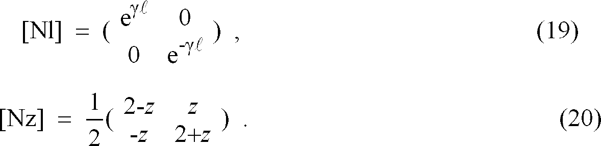
- the product of the electrical propagation constant ⁇ and the mechanical length l of the line used is calculated in the subsequent calculation, since this product ⁇ l is required for the calibration according to the 7-term method.
- the mechanical length of the line can also be unknown for the calibration.
- ⁇ l can also be determined in a simple manner from this calculated product ⁇ if the mechanical length of the line used is known.
- the method according to the invention is particularly suitable for on-wafer measurements in which the two measuring gates end in the measuring tips, which are not placed too closely next to one another directly on the conductor tracks of the semiconductor substrate and are therefore not yet coupled to one another.
- NWA network analyzer
- these measuring branches open into two four-port gates 4 and 5, of which a linear transmission behavior and additionally a decoupling of the measuring points 8 and 9 or 10 and 11 are required.
- these four gates have all-round adaptation and the structure of a bridge, so that, for example, the measuring point 8 forms a measure for the incoming wave from the branch 12 and the measuring point 9 forms a measure for the wave approaching from the test object 3 .
- impedance parameters such a low-resistance test set can be unfavorable.
- any linear description of networks can be adopted by using a system error correction method.
- the measuring gates 6 and 7 form the transition to the test object 3 and are also referred to as reference planes.
- the so-called two-port error model (7-term model) the disturbances occurring between the measuring points 8, 9, 10 and 11 and the measuring object 3 connected to the actual measuring gates 6 and 7 are caused by mismatches, for example due to the connecting lines leading to the measuring object and undesired coupling are caused by so-called error networks, which are determined by a calibration method and are taken into account as correction values during the actual measurement.
- test object 3 is replaced by calibration standards and four measured values are then again recorded for each switch position of the changeover switch 2 per standard.
- the mathematical derivation is to be carried out in a general form based on FIG. 1, so that both chain and transmission parameters could be used.
- the electrical quantities at the measuring points are treated like general measured values, which can represent either currents and voltages or wave quantities.
- the matrices [ A ] and [ B ] are error matrices that result from the so-called four-port two-port reduction.
- the physical quantities of the DUT which is described by the matrix [ N ], are transformed to the measuring points via these matrices.
- the LZY method is not only a good alternative to the LRM method for on-wafer measurements, but can also be regarded as the next step in the area of self-calibration methods for on-wafer measurements in the case of a crosstalk-free system.
- the calibration standards of the LZN method according to the invention are shown in FIG. 3.
- the calibration line must have adjustment as usual.
- the spread constant However, ⁇ need not be known.
- the impedance value of the Z standard represents the reference impedance.
- the N standard only requires reflection symmetry.
- the LMS process is very closely related to the LRM process.
- the difference between these two methods is that in the LMS method the line may have an unknown propagation constant and the reflection standard, in contrast to the LRM method, must be known.
- the LMS method only has an unknown self-calibration variable.
- This unknown transmission value of the line can be determined, among other things, by setting up the homogeneous 8 * 8 system of equations for determining the error coefficients consisting of the four equations for the line standard and the two equations for the reflection standards, and that the system of equations by numerical variation of the Self-calibration size manipulated in this way becomes that its determinant value gives the value zero necessary for homogeneous systems of equations.
Landscapes
- Physics & Mathematics (AREA)
- General Physics & Mathematics (AREA)
- Measurement Of Resistance Or Impedance (AREA)
- Investigating Or Analysing Materials By Optical Means (AREA)
Abstract
Description
Die Erfindung geht aus von einem Verfahren laut Oberbegriff des Hauptanspruches.The invention is based on a method according to the preamble of the main claim.
Ein Verfahren dieser Art ist bekannt (DE 39 12 795 bzw. korrespondierende US-PS 4.982.164). Dieses sogenannte 7-Term-Verfahren besitzt den Vorteil, daß nur drei Kalibrierstandards benötigt werden. Nach dem bekannten Verfahren wird allerdings für die erste Kalibriermessung ein Zweitor vorausgesetzt, von dem sämtliche komplexen Streuparameter bekannt sind. Dies wird für Objektmessungen im koaxialen Wellenleiterbereich am einfachsten durch eine direkte Verbindung der beiden Meßtore (Through-Messung) erreicht, für die zweite Kalibriermessung wird beispielsweise ein reflexionsfreier Wellensumpf (Match) nacheinander an die beiden Meßtore angeschlossen, für die dritte Kalibriermessung wird beispielsweise ein Eintor bekannter Reflexion (Reflexion) nacheinander an die beiden Meßtore angeschlossen (TMR-Kalibrierverfahren genannt). Für Messungen auf planaren Mikrowellenschaltungen oder Halbleitersubstraten (On-Wafer-Messungen) ist der T-Standard meist nicht mehr realisierbar, hier wird stattdessen eine bekannte Leitung (Line) als erster Kalibrierstandard für die erste Messung benutzt (LRM-Kalibrierung beispielsweise auch beschrieben in "Achieving greater on-wafer S-parameter accuracy with the LRM calibration technique", von A. Davidson, E. Strid und K. Jones, Cascade-Microtech, Product Note). Auch dieses bekannte inzwischen für On-Wafer-Messungen benutzte LRM-Kalibrierverfahren setzt voraus, daß sämtliche Streuparameter der für die erste Kalibriermessung benutzten elektrischen Leitung bekannt sind, also sowohl der Wellenwiderstand als auch die komplexe Ausbreitungskonstante bzw. das Produkt der komplexen Ausbreitungskonstante mit der mechanischen Länge der Leitung. Der erste Kalibrierstandard für dieses bekannte Verfahren ist daher relativ aufwendig und teuer.A method of this type is known (DE 39 12 795 or corresponding US Pat. No. 4,982,164). This so-called 7-term method has the advantage that only three calibration standards are required. According to the known method, however, a two-port is required for the first calibration measurement, from which all complex scattering parameters are known. This is for object measurements in the coaxial waveguide region most easily by a direct connection of two measuring ports (T hrough measurement) achieved for the second calibration measurement is a reflection-free wave sink (M atch) successively, for example, connected to the two measuring ports, the third calibration measurement is, for example, a one-port reflection known (R eflexion) connected to the two measuring ports in succession (TMR-called calibration). For measurements on planar microwave circuits or semiconductor substrates (on-wafer measurements) is the T standard usually not feasible here instead, a well-known line (L ine) will be the first calibration for the first measurement used (LRM calibration for example, described in "Achieving greater on-wafer S-parameter accuracy with the LRM calibration technique" , by A. Davidson, E. Strid and K. Jones, Cascade-Microtech, Product Note). This known LRM calibration method, which is now used for on-wafer measurements, also requires that all scattering parameters of the electrical line used for the first calibration measurement are known, i.e. both the characteristic impedance and the complex propagation constant or the product of the complex propagation constant with the mechanical one Length of the line. The first calibration standard for this known method is therefore relatively complex and expensive.
Es ist Aufgabe der Erfindung, ein Kalibrierverfahren nach dem 7-Term-Prinzip aufzuzeigen, bei dem drei einfache und preiswerte Kalibrierstandards benutzt werden können.It is an object of the invention to demonstrate a calibration method based on the 7-term principle, in which three simple and inexpensive calibration standards can be used.
Diese Aufgabe wird ausgehend von einem Verfahren laut Oberbegriff des Hauptanspruches durch dessen kennzeichnende Merkmale gelöst. Vorteilhafte Weiterbildungen ergeben sich aus den Unteransprüchen.This object is achieved on the basis of a method according to the preamble of the main claim by its characterizing features. Advantageous further developments result from the subclaims.
Die Erfindung geht aus von der Erkenntnis, daß von der für die erste Kalibriermessung benutzten elektrischen Leitung nur der Wellenwiderstand bekannt sein muß, während die elektrische Ausbreitungskonstante unbekannt und komplex sein darf, da diese anschließend aus sämtlichen Kalibriermessungen auf einfache Weise berechnet werden kann, wie dies nachfolgend näher beschrieben wird (Formel 16). Damit kann der erste Kalibrierstandard sehr einfach und preiswert realisiert werden. Eine solche kurze elektrische Leitung, von der nur der Wellenwiderstand bekannt ist, nicht aber die Ausbreitungskonstante, kann vor allem auch sehr einfach und preiswert in planarer Streifenleitungstechnik aufgebaut werden, ein solcher Kalibrierstandard ist damit besonders geeignet zur Kalibrierung für anschließende Objektmessungen an planaren Mikrowellenschaltungen (On-Wafer-Messungen). Die Kalibrierstandards für die zweite und dritte Kalibriermessung können ebenfalls sehr einfach und preiswert realisiert werden, wie dies Gegenstand der Unteransprüche ist.The invention is based on the knowledge that only the characteristic impedance of the electrical line used for the first calibration measurement has to be known, while the electrical propagation constant may be unknown and complex, since this then consists of all Calibration measurements can be calculated in a simple manner, as described in more detail below (Formula 16). The first calibration standard can thus be implemented very simply and inexpensively. Such a short electrical line, of which only the wave resistance is known, but not the propagation constant, can above all also be constructed very simply and inexpensively using planar stripline technology; such a calibration standard is therefore particularly suitable for calibration for subsequent object measurements on planar microwave circuits (On Wafer measurements). The calibration standards for the second and third calibration measurements can also be implemented very simply and inexpensively, as is the subject of the subclaims.
Bei dem sogenannten LZY-Verfahren wird für die zweite und dritte Kalibriermessung jeweils der gleiche Kalibrierstandard benutzt, der aus einer bekannten Serienimpedanz und einer unbekannten Impedanz gegen Masse besteht. Serienimpedanzen lassen sich auch in planaren Mikrowellenschaltungen mit großer Präzision und geringen parasitären Anteilen anfertigen, während die Fertigung von präzisen Impedanzen gegen Masse im besonderen auf Halbleitersubstraten nicht möglich ist. Dieser ZY-Kalibrierstandard bietet ferner noch den Vorteil, daß der Eingangswiderstand des einen Tores auf den Bezugswiderstand (im allgemeinen 50 Ohm) ausgelegt werden kann, was eine Meßempfindlichkeit für diesen wichtigen Impedanzwert garantiert. Zur Selbstkontrolle des Kalibrierprozesses kann bei dieser LZY-Kalibriermessung gegebenenfalls auch anschließend noch der Wert der Y-Komponente aus den Meßwerten berechnet werden.In the so-called LZY method, the same calibration standard is used for the second and third calibration measurement, which consists of a known series impedance and an unknown impedance to ground. Series impedances can also be produced in planar microwave circuits with great precision and low parasitic components, while it is not possible to produce precise impedances to ground, in particular on semiconductor substrates. This ZY calibration standard also has the advantage that the input resistance of one gate can be designed for the reference resistance (generally 50 ohms), which guarantees a measuring sensitivity for this important impedance value. For self-control of the calibration process, the value of the Y component can also be subsequently calculated from the measured values in this LZY calibration measurement.
Bei dem LZN-Verfahren nach Unteranspruch 4 und 5 wird für die zweite Kalibriermessung ein Zweitor benutzt, das nur aus einer Serienimpedanz besteht, ein solcher Kalibrierstandard kann noch einfacher und preiswerter aufgebaut werden. Da die Impedanz gegen Masse entfällt, besitzt dieser Z-Standard von tiefsten bis zu sehr hohen Frequenzen ein äußerst homogenes Verhalten. Der zusätzlich noch verwendete N-Standard liefert noch zusätzlich Selbstkalibrierwerte für das Transmissionsverhalten, so daß dieses LZN-Verfahren die Möglichkeit bietet, über eine Vorabinformation des N-Standards die Meßfähigkeit sowohl für Relexionsmessungen als auch für Transmissionsmessungen zu sichern.In the LZN method according to
Bei dem LZZN-Verfahren nach Anspruch 5 sind zwar insgesamt vier Kalibriermessungen zur Ermittlung der sieben Fehlerterme nötig, von den beiden Z-Standards, die wiederum nur einen Serienwiderstand aufweisen, muß jedoch lediglich der Realteil des Impedanzwertes bekannt sein, so daß von einer Impedanz, die sich beispielsweise aus ohmschen Anteil und Serieninduktivität zusammensetzt, nur noch der bei niedrigen Frequenzen leicht ermittelbare ohmsche Anteil bekannt sein muß. Damit kann der Z-Standard noch einfacher und preiswerter aufgebaut werden.In the LZZN method according to
Bei dem LMS- bzw. LMO-Kalibrierverfahren nach Unteranspruch 6 werden für die zweite und dritte Kalibriermessung an sich bekannte Eintor-Kalibrierstandards benutzt, nämlich ein Eintor in Form eines Wellensumpfes M, dessen Impedanz dem Bezugswiderstand (Wellenwiderstand) entspricht und das nacheinander an die beiden Meßtore angeschaltet wird (sogenannte Doppeleintor-Kalibrierung MM). Für die dritte Kalibriermessung wird wieder eine Doppeleintor-Kalibrierung mit einem Kurzschluß (SS) oder Lehrlauf (OO) durchgeführt. Damit können kommerziell erhältliche Kalibriersubstrate für die zweite und dritte Kalibriermessung benutzt werden.In the LMS or LMO calibration method according to
Gemäß der nachfolgenden Beschreibung im Zusammenhang mit Gleichung (16) wird bei der anschließenden Berechnung das Produkt von elektrischer Ausbreitungskonstante γ und mechanischer Länge l der verwendeten Leitung berechnet, da für die Kalibrierung nach dem 7-Term-Verfahren dieses Produkt γℓ benötigt wird. Für die Kalibrierung kann also auch die mechanische Länge der Leitung unbekannt sein. Nachdem für die anschließende Objektmessung jedoch oftmals nur die komplexe Ausbreitungskonstante γ von Interesse ist, beispielsweise für die Einstellung der Referenzebene, kann aus diesem berechneten Produkt γℓ bei Kenntnis der mechanischen Länge der verwendeten Leitung auf einfache Weise auch unmittelbar γ ermittelt werden.According to the following description in connection with equation (16), the product of the electrical propagation constant γ and the mechanical length l of the line used is calculated in the subsequent calculation, since this product γℓ is required for the calibration according to the 7-term method. The mechanical length of the line can also be unknown for the calibration. However, since often only the complex propagation constant γ is of interest for the subsequent object measurement, for example for the setting of the reference plane, γℓ can also be determined in a simple manner from this calculated product γ if the mechanical length of the line used is known.
Das erfindungsgemäße Verfahren ist besonders geeignet für On-Wafer-Messungen, bei denen die beiden Meßtore in den Meßspitzen enden, die unmittelbar auf den Leiterbahnen des Halbleitersubstrats nicht zu eng nebeneinander aufgesetzt werden und daher noch nicht miteinander verkoppelt sind.The method according to the invention is particularly suitable for on-wafer measurements in which the two measuring gates end in the measuring tips, which are not placed too closely next to one another directly on the conductor tracks of the semiconductor substrate and are therefore not yet coupled to one another.
Die Erfindung wird im folgenden anhand schematischer Zeichnungen an Ausführungsbeispielen näher erläutert.The invention is explained below with reference to schematic drawings of exemplary embodiments.
Fig. 1 zeigt ein stark vereinfachtes Prinzipschaltbild eines Netzwerkanalysators (NWA), bei dem über einen Umschalter 2 zwei Meßzweige 12 und 13 aus einem Hochfrequenzgenerator 1 gespeist sind. Diese Meßzweige münden in zwei Viertoren 4 und 5, von denen ein lineares Übertragungsverhalten und zusätzlich eine Entkopplung der Meßstellen 8 und 9 bzw. 10 und 11 verlangt wird. Im Falle vom Streuparametermessungen ist es vorteilhaft, wenn diese Viertore allseitige Anpassung und die Struktur einer Brücke aufweisen, so daß beispielsweise die Meßstelle 8 ein Maß für die hinlaufende Welle aus dem Zweig 12 und die Meßstelle 9 ein Maß für die vom Meßobjekt 3 zulaufende Welle bildet. Möchte man jedoch Impedanzparameter aufnehmen, so kann ein derartiges niederohmiges Testset ungünstig sein. Wie auch immer, sofern die Entkopplung der Meßstellen und ein lineares Übertragungsverhalten der Viertore 4 und 5 des Testsets gesichert sind, kann durch Einsatz eines Systemfehlerkorrekturverfahrens auf jede lineare Beschreibungsform von Netzwerken übergegangen werden.1 shows a very simplified basic circuit diagram of a network analyzer (NWA), in which two measuring
Die Meßtore 6 und 7 bilden den Übergang zu dem Meßobjekt 3 und werden auch als Referenzebenen bezeichnet. Nach dem sogenannten Zweitor-Fehlermodell (7-Term Modell) werden hierbei die zwischen den Meßpunkten 8, 9, 10 und 11 und dem an den eigentlichen Meßtoren 6 und 7 angeschalteten Meßobjekt 3 auftretenden Störgrößen, die beispielsweise durch die zum Meßobjekt führenden Verbindungsleitungen, Fehlanpassungen und unerwünschte Verkopplungen verursacht werden, durch sogenannte Fehlernetzwerke berücksichtigt, die durch ein Kalibrierverfahren ermittelt und bei der eigentlichen Messung als Korrekturwerte berücksichtigt werden.The
Bei der Kalibriermessung wird das Meßobjekt 3 durch Kalibrierstandards ersetzt und es werden dann wiederum pro Standard vier Meßwerte für jede Schalterstellung des Umschalters 2 erfaßt.During the calibration measurement, the
Zur Veranschaulichung der folgenden Zweitor-Selbstkalibrierverfahren LZY, LZN, LZZN und LMS ist es unabdingbar die Abbildungsgleichung der 7-Term-Verfahren kurz herzuleiten.To illustrate the following two-port self-calibration procedures LZY, LZN, LZZN and LMS, it is essential to derive the mapping equation for the 7-term procedure briefly.
Im weiteren soll die mathematische Herleitung in allgemeiner Form basierend auf Fig. 1 erfolgen, so daß sowohl Ketten- als auch Transmissionsparameter einsetzbar wären. Behandelt werden die elektrischen Größen an den Meßstellen wie allgemeine Meßwerte, die entweder Ströme und Spannungen oder Wellengrößen repräsentieren können. Die mathematische Formulierung des Zweitor-Fehlermodells wird in Ketten- bzw. Transmissionsparametern angesetzt:![]()
![]()
Für jede Schalterstellung des im Fig. 1 dargestellten NWA, der auch als Doppelreflektometer bezeichnet wird, erhält man eine sinnvolle Gleichung, die vereint die folgende Matrizengleichung ergibt.![]()
![]()
![]()


![]()
![]()
![]()
![]()

Die Auswertung dieser Gleichung bringt das gesuchte Produkt γℓ hervor.
- Bei dem LRM-Verfahren muß die Leitung komplett bekannt sein, hingegen muß beim LZY-Verfahren nur eine angepaßte Leitung eingesetzt werden.
- Die bekannte Bezugsimpedanz liegt bei dem LRM-Verfahren gegen Masse, hingegen liegt diese bei dem LZY-Verfahren planar in Serie, was einer präzisen Herstellbarkeit zugute kommt.
- Da sich der Z-Standard einfacher herstellen läßt als der M-Standard, ist dieser ZY-Standard auch bis zu höheren Frequenzen gut realisierbar.
- Die zwei Kalibrierstandards des LZY-Verfahrens benötigen weniger Platz als die Standards des LRM-Verfahren, was insbesondere bei der Herstellung auf teueren Halbleitersubstraten sehr wichtig ist.
The evaluation of this equation produces the product γℓ we are looking for.
- With the LRM method, the line must be completely known, whereas with the LZY method, only an adapted line must be used.
- The known reference impedance lies with the LRM method against ground, whereas with the LZY method this is in series in plan, which benefits precise producibility.
- Since the Z standard is easier to manufacture than the M standard, this ZY standard can also be easily implemented up to higher frequencies.
- The two calibration standards of the LZY process take up less space than the standards of the LRM process, which is very important particularly when manufacturing on expensive semiconductor substrates.
Somit ist es offensichtlich, daß für on-wafer-Messungen das LZY-Verfahren nicht nur eine gute Alternative zum LRM-Verfahren darstellt, sondern als nächster Schritt im Bereich der Selbstkalibrierverfahren für on-wafer-Messungen im übersprecherfreien Fall angesehen werden darf.It is therefore obvious that the LZY method is not only a good alternative to the LRM method for on-wafer measurements, but can also be regarded as the next step in the area of self-calibration methods for on-wafer measurements in the case of a crosstalk-free system.
Die Kalibrierstandards des erfindungsgemäßen LZN-Verfahrens sind im Fig. 3 abgebildet. Die Kalibrierleitung muß wie üblich Anpassung aufweisen. Die Ausbreitungskonstante γ muß jedoch nicht bekannt sein. Der Impedanzwert des Z-Standards stellt die Bezugsimpedanz dar. Von dem N-Standard wird lediglich Reflexionssymmetrie gefordert. Zunächst beschäftigen wir uns für die Berechnung der Ausbreitungskonstante lediglich mit den Standards L und Z. Diese beiden Standards ergeben in Referenz zur Gleichung (3) in Transmissionsparametern:
![]()
![]()

![]()
![]()
Widmen wir uns an dieser Stelle dem dritten Kalibrierstandard N, der die drei unbekannten Streuparametergrößen Sn₁₁, Sn₁₂ und Sn₂₁ aufweisen soll. Damit dieser reflexionssymmetrische Standard auch aus denen in der Praxis wichtigen Eintor-Standards bestehen kann, ist ein Übergang zu den sogenannten Pseudotransmissionsparametern notwendig. Für diesen Übergang zerlegen wir die Meßwertmatrix der Gleichung (4) wie folgt.
Dieser Schritt ist notwendig, da bei einem Doppeleintor-Kalibrierstandard m nx zu Null wird. Ordnen wir dem physikalischen Parametern des N-Standards diese Meßwertdeterminante zu, so läßt sich für den dritten Standard die Gleichung (3) derartig formulieren:
Die Größen des Hetzwerks [Nn'] stehen in folgenden Zusammenhang mit den Streuparametern.


This step is necessary because with a double one-port calibration standard, m nx becomes zero. If we assign this measured value determinant to the physical parameters of the N standard, then equation (3) can be formulated in this way for the third standard:
The sizes of the rush [ Nn '] are related to the scattering parameters.
Die Tatsache, daß auch noch bei dem LZN-Verfahren der Serienwiderstand vollständig bekannt sein muß, kann mitunter zu Problemen führen. Abhilfe schafft bezüglich dieser Problematik das LZZN-Verfahren. Zur Durchführung dieses Verfahrens werden zwei unterschiedliche Serienwiderstände benötigt.The fact that the series resistance must also be fully known in the LZN process can sometimes lead to problems. The LZZN procedure provides a remedy for this problem. Two different series resistors are required to carry out this process.
Von diesen beiden Widerständen soll nur noch jeweils der Realteil bekannt sein. Die Imaginärteile sind nunmehr die gesuchten Größen eines weiteren Selbstkalibrierschrittes. Stellt man Gleichung (22) für beide Widerstände auf und setzt unter Eliminierung von eγℓ diese beiden Gleichung gleich, so verfügt man über eine komplexe nichtlineare Gleichung zur Ermittlung der beiden Imaginärteile. Folglich läßt sich diese Gleichung nur noch numerisch auswerten.Of these two resistors, only the real part should be known. The imaginary parts are now the desired sizes of a further self-calibration step. If one sets up equation (22) for both resistors and equates these two equations while eliminating e γℓ , then one has a complex non-linear equation for determining the two imaginary parts. As a result, this equation can only be evaluated numerically.
Das LMS-Verfahren steht in sehr enger Verwandtschaft zu dem LRM-Verfahren. Diese beiden Verfahren unterscheiden sich dadurch, daß bei dem LMS-Verfahren die Leitung eine unbekannte Ausbreitungskonstante aufweisen darf und der Reflexionsstandard in Gegensatz zum LRM-Verfahren bekannt sein müssen. Somit weist das LMS-Verfahren genauso wie auch das LRM-Verfahren nur eine unbekannte Selbstkalibriergröße auf. Die Ermittlung dieses unbekannten Transmissionswertes der Leitung kann unter anderem dadurch erfolgen, daß das homogene 8 * 8 Gleichungssystem zur Ermittlung der Fehlerkoeffizienten bestehend aus den vier Gleichungen für den Leitungsstandard und den jeweils zwei Gleichungen für die Reflexionsstandards aufgestellt wird und daß das Gleichungssystem durch numerische Variation der Selbstkalibriergröße derart manipuliert wird, daß dessen Determinantenwert den für homogene Gleichungssysteme notwendigen Wert Null ergibt.The LMS process is very closely related to the LRM process. The difference between these two methods is that in the LMS method the line may have an unknown propagation constant and the reflection standard, in contrast to the LRM method, must be known. Thus, just like the LRM method, the LMS method only has an unknown self-calibration variable. This unknown transmission value of the line can be determined, among other things, by setting up the homogeneous 8 * 8 system of equations for determining the error coefficients consisting of the four equations for the line standard and the two equations for the reflection standards, and that the system of equations by numerical variation of the Self-calibration size manipulated in this way becomes that its determinant value gives the value zero necessary for homogeneous systems of equations.
Danach können in herkömmlicher Art und Weise mit dem inhomogenen 7*7 Gleichungssystem die 7 Fehlerterme bestimmt werden.Then the 7 error terms can be determined in a conventional manner with the inhomogeneous 7 * 7 system of equations.
Claims (6)
und die dritte Kalibriermessung an einem reflexionssymmetrischen Zweitor durchgeführt wird, dessen Impedanz unbekannt sein darf.Method according to Claim 1 or 2, characterized in that the second calibration measurement is carried out on a two-port system which consists of only a single concentrated component of known impedance which is connected in series
and the third calibration measurement is carried out on a reflection-symmetrical two-port, the impedance of which may be unknown.
wobei vor der dritten Kalibriermessung an dem reflexionssymmetrischen Zweitor unbekannter Impedanz eine weitere Kalibriermessung an einem Zweitor durchgeführt wird, das wiederum nur aus einem einzigen konzentrierten in Serie geschalteten Bauelement bekannter Resistanz jedoch unbekannter Reaktanz besteht und dessen Resistanzwert sich von dem des Kalibrierstandards der zweiten Kalibriermessung unterscheidet.Method according to Claim 4, characterized in that the second calibration measurement is carried out on a two-port, of which only the resistance of the component connected in series is known and of which the reactance may be unknown,
wherein before the third calibration measurement on the reflection-symmetrical two-port of unknown impedance, another calibration measurement is carried out on a two-port, which in turn consists of only one concentrated series-connected component of known resistance but unknown reactance and whose resistance value differs from that of the calibration standard of the second calibration measurement.
und
die dritte Kalibriermessung an einem weiteren Eintor durchgeführt wird, das bekannte Reflexion besitzt und nacheinander an die beiden Meßtore angeschaltet wird.Method according to claim 1 or 2, characterized in that the second calibration measurement is carried out with a one-port whose wave resistance is known and which is switched on in succession to the two measuring ports,
and
the third calibration measurement is carried out on a further one-port, which has known reflection and is successively connected to the two measuring ports.
Applications Claiming Priority (2)
| Application Number | Priority Date | Filing Date | Title |
|---|---|---|---|
| DE4435559A DE4435559A1 (en) | 1994-10-05 | 1994-10-05 | Procedure for performing electrical precision measurements with self-control |
| DE4435559 | 1994-10-05 |
Publications (3)
| Publication Number | Publication Date |
|---|---|
| EP0706055A2 true EP0706055A2 (en) | 1996-04-10 |
| EP0706055A3 EP0706055A3 (en) | 1996-05-22 |
| EP0706055B1 EP0706055B1 (en) | 2001-12-05 |
Family
ID=6529997
Family Applications (2)
| Application Number | Title | Priority Date | Filing Date |
|---|---|---|---|
| EP95115297A Expired - Lifetime EP0706055B1 (en) | 1994-10-05 | 1995-09-28 | Method for calibrating a network analyzer according to the 7-term principle |
| EP95115296A Expired - Lifetime EP0706059B1 (en) | 1994-10-05 | 1995-09-28 | Calibrating procedure for a network analyzer using the 15-term principle |
Family Applications After (1)
| Application Number | Title | Priority Date | Filing Date |
|---|---|---|---|
| EP95115296A Expired - Lifetime EP0706059B1 (en) | 1994-10-05 | 1995-09-28 | Calibrating procedure for a network analyzer using the 15-term principle |
Country Status (4)
| Country | Link |
|---|---|
| US (2) | US5608330A (en) |
| EP (2) | EP0706055B1 (en) |
| DE (3) | DE4435559A1 (en) |
| ES (2) | ES2168327T3 (en) |
Families Citing this family (32)
| Publication number | Priority date | Publication date | Assignee | Title |
|---|---|---|---|---|
| US5561378A (en) * | 1994-07-05 | 1996-10-01 | Motorola, Inc. | Circuit probe for measuring a differential circuit |
| US5748506A (en) * | 1996-05-28 | 1998-05-05 | Motorola, Inc. | Calibration technique for a network analyzer |
| DE19639515B4 (en) * | 1996-09-26 | 2006-10-12 | Rosenberger Hochfrequenztechnik Gmbh & Co. | Arrangement for calibrating a network analyzer for on-wafer measurement on integrated microwave circuits |
| TW346541B (en) * | 1997-10-15 | 1998-12-01 | Ind Tech Res Inst | Method for calibrating stepper attenuator a method for calibrating a stepper attenuator, comprises testing the S parameters with no attenuator; separately testing the S parameters for each attenuator; etc. |
| DE19743712C2 (en) * | 1997-10-02 | 2003-10-02 | Rohde & Schwarz | Method for calibrating a vector network analyzer having two measuring gates and four measuring points according to the 15-term error model |
| US6060888A (en) * | 1998-04-24 | 2000-05-09 | Hewlett-Packard Company | Error correction method for reflection measurements of reciprocal devices in vector network analyzers |
| US6188968B1 (en) * | 1998-05-18 | 2001-02-13 | Agilent Technologies Inc. | Removing effects of adapters present during vector network analyzer calibration |
| US6300775B1 (en) | 1999-02-02 | 2001-10-09 | Com Dev Limited | Scattering parameter calibration system and method |
| US6421624B1 (en) * | 1999-02-05 | 2002-07-16 | Advantest Corp. | Multi-port device analysis apparatus and method and calibration method thereof |
| GB2347754A (en) * | 1999-03-11 | 2000-09-13 | Alenia Marconi Syst Ltd | Measuring electromagnetic energy device parameters |
| US6230106B1 (en) * | 1999-10-13 | 2001-05-08 | Modulation Instruments | Method of characterizing a device under test |
| US6571187B1 (en) * | 2000-02-09 | 2003-05-27 | Avaya Technology Corp. | Method for calibrating two port high frequency measurements |
| US6342947B1 (en) * | 2000-04-10 | 2002-01-29 | The United States Of America As Represented By The Secretary Of The Army | Optical power high accuracy standard enhancement (OPHASE) system |
| US6590644B1 (en) * | 2001-01-12 | 2003-07-08 | Ciena Corporation | Optical module calibration system |
| US6643597B1 (en) * | 2001-08-24 | 2003-11-04 | Agilent Technologies, Inc. | Calibrating a test system using unknown standards |
| JP3558074B2 (en) * | 2001-12-10 | 2004-08-25 | 株式会社村田製作所 | Method of correcting measurement error, method of determining quality of electronic component, and electronic component characteristic measuring device |
| US7064555B2 (en) * | 2003-02-18 | 2006-06-20 | Agilent Technologies, Inc. | Network analyzer calibration employing reciprocity of a device |
| US7107170B2 (en) * | 2003-02-18 | 2006-09-12 | Agilent Technologies, Inc. | Multiport network analyzer calibration employing reciprocity of a device |
| GB2409049B (en) * | 2003-12-11 | 2007-02-21 | Agilent Technologies Inc | Power measurement apparatus and method therefor |
| DE102005005056B4 (en) | 2004-09-01 | 2014-03-20 | Rohde & Schwarz Gmbh & Co. Kg | Method for calibrating a network analyzer |
| US8126670B2 (en) * | 2006-06-21 | 2012-02-28 | Rohde & Schwarz Gmbh & Co. Kg | Method and device for calibrating a network analyzer for measuring at differential connections |
| DE102006030630B3 (en) * | 2006-07-03 | 2007-10-25 | Rosenberger Hochfrequenztechnik Gmbh & Co. Kg | High frequency measuring device e.g. vector network analyzer, calibrating method, involves comparing value of scattering parameters determined for all pair wise combination with value described for calibration standard |
| US7532014B2 (en) * | 2006-08-08 | 2009-05-12 | Credence Systems Corporation | LRL vector calibration to the end of the probe needles for non-standard probe cards for ATE RF testers |
| US7777497B2 (en) * | 2008-01-17 | 2010-08-17 | Com Dev International Ltd. | Method and system for tracking scattering parameter test system calibration |
| US8436626B2 (en) * | 2009-12-17 | 2013-05-07 | Taiwan Semiconductor Manfacturing Company, Ltd. | Cascaded-based de-embedding methodology |
| CN101782637B (en) * | 2010-03-16 | 2013-04-03 | 南京航空航天大学 | Radio frequency current probe characteristic calibrating method based on electromagnetic compatibility analysis and application |
| US8798953B2 (en) * | 2011-09-01 | 2014-08-05 | Yuan Ze University | Calibration method for radio frequency scattering parameter measurement applying three calibrators and measurement structure thereof |
| DE102012006314A1 (en) * | 2012-03-28 | 2013-10-02 | Rosenberger Hochfrequenztechnik Gmbh & Co. Kg | Time domain measurement with calibration in the frequency domain |
| CN103543425B (en) * | 2013-10-28 | 2016-06-29 | 中国电子科技集团公司第四十一研究所 | A kind of method of automatic compensation Network Analyzer measuring surface variation error |
| US20160146920A1 (en) * | 2014-11-20 | 2016-05-26 | Sigurd Microelectronics Corp. | Rf parameter calibration method |
| DE102014019008B4 (en) | 2014-12-18 | 2022-05-05 | Rosenberger Hochfrequenztechnik Gmbh & Co. Kg | Procedure for calibrating a measurement adaptation with two differential interfaces |
| US10890642B1 (en) | 2019-07-31 | 2021-01-12 | Keysight Technologies, Inc. | Calibrating impedance measurement device |
Citations (2)
| Publication number | Priority date | Publication date | Assignee | Title |
|---|---|---|---|---|
| DE3912795A1 (en) | 1988-04-22 | 1989-11-02 | Rohde & Schwarz | Method for calibrating a network analyser |
| US4982164A (en) | 1988-04-22 | 1991-01-01 | Rhode & Schwarz Gmbh & Co. K.G. | Method of calibrating a network analyzer |
Family Cites Families (4)
| Publication number | Priority date | Publication date | Assignee | Title |
|---|---|---|---|---|
| DE3911254A1 (en) * | 1989-04-07 | 1990-10-11 | Eul Hermann Josef Dipl Ing | Method for establishing the complex measuring capability of homodyne network analysers |
| US5313166A (en) * | 1990-11-11 | 1994-05-17 | Rohde & Schwarz Gmbh & Co. Kg | Method of calibrating a network analyzer |
| EP0568889A3 (en) * | 1992-05-02 | 1994-06-22 | Berthold Lab Prof Dr | Process for calibrating a network analyser |
| DE4332273C2 (en) | 1992-12-12 | 1997-09-25 | Rohde & Schwarz | Procedure for calibrating a network analyzer |
-
1994
- 1994-10-05 DE DE4435559A patent/DE4435559A1/en not_active Ceased
-
1995
- 1995-09-28 ES ES95115296T patent/ES2168327T3/en not_active Expired - Lifetime
- 1995-09-28 EP EP95115297A patent/EP0706055B1/en not_active Expired - Lifetime
- 1995-09-28 DE DE59509963T patent/DE59509963D1/en not_active Expired - Lifetime
- 1995-09-28 ES ES95115297T patent/ES2164128T3/en not_active Expired - Lifetime
- 1995-09-28 EP EP95115296A patent/EP0706059B1/en not_active Expired - Lifetime
- 1995-09-28 DE DE59509906T patent/DE59509906D1/en not_active Expired - Lifetime
- 1995-10-04 US US08/539,087 patent/US5608330A/en not_active Expired - Lifetime
- 1995-10-04 US US08/539,086 patent/US5666059A/en not_active Expired - Lifetime
Patent Citations (2)
| Publication number | Priority date | Publication date | Assignee | Title |
|---|---|---|---|---|
| DE3912795A1 (en) | 1988-04-22 | 1989-11-02 | Rohde & Schwarz | Method for calibrating a network analyser |
| US4982164A (en) | 1988-04-22 | 1991-01-01 | Rhode & Schwarz Gmbh & Co. K.G. | Method of calibrating a network analyzer |
Also Published As
| Publication number | Publication date |
|---|---|
| EP0706059A1 (en) | 1996-04-10 |
| EP0706055B1 (en) | 2001-12-05 |
| ES2168327T3 (en) | 2002-06-16 |
| US5666059A (en) | 1997-09-09 |
| EP0706055A3 (en) | 1996-05-22 |
| DE4435559A1 (en) | 1996-04-11 |
| US5608330A (en) | 1997-03-04 |
| EP0706059B1 (en) | 2001-12-19 |
| DE59509963D1 (en) | 2002-01-31 |
| ES2164128T3 (en) | 2002-02-16 |
| DE59509906D1 (en) | 2002-01-17 |
Similar Documents
| Publication | Publication Date | Title |
|---|---|---|
| EP0706055B1 (en) | Method for calibrating a network analyzer according to the 7-term principle | |
| DE4332273C2 (en) | Procedure for calibrating a network analyzer | |
| EP3039443B1 (en) | Method for calibrating a measurement setup | |
| DE102004020037B4 (en) | Calibration method for performing multi-port measurements on semiconductor wafers | |
| DE4017412C2 (en) | Testing device and its use in a device for measuring s-parameters of a test object | |
| EP0793110B1 (en) | Method for measuring an electronic object with a network analyser | |
| EP2156202B1 (en) | Method and device for the calibration of network analyzers using a comb generator | |
| DE102007027142B4 (en) | Method and device for calibrating a network analyzer for measurements on differential connections | |
| DE4313705C2 (en) | Method for calibrating a network analyzer and calibration devices for carrying out the method | |
| DE2262053C3 (en) | Method for determining the electrical parameters of a transistor | |
| DE112007002891B4 (en) | Method and apparatus for correcting a high frequency characteristic error of electronic components | |
| DE19722471C2 (en) | Impedance and current measuring device | |
| DE3912795C2 (en) | ||
| DE19918697B4 (en) | Calibration method for performing multi-port measurements based on the 10-term method | |
| DE4433375C2 (en) | Procedure for calibrating a network analyzer | |
| DE4404046C2 (en) | Method for calibrating a network analyzer with two measuring gates | |
| DE10242932B4 (en) | The LRR method for calibrating vectorial 4-terminal network analyzers | |
| DE19736897A1 (en) | Calibration method for vectorial network channel analyser | |
| DE102014019008B4 (en) | Procedure for calibrating a measurement adaptation with two differential interfaces | |
| DE102007057394A1 (en) | Vector network analyzer calibrating method, involves implementing reflection standards resembling short-circuit and open-circuit operation in which ports are physically equal, and realizing transmission values of port by through connection | |
| DE102005013583B4 (en) | Method for measuring the scattering parameters of multi-ports with 2-port network analyzers and corresponding measuring device | |
| DE4405211A1 (en) | Method for calibrating a network analyser having two measuring ports and three measuring positions | |
| DE102004012217B4 (en) | LR1R2 method for calibration of vector network analyzers and corresponding calibration device | |
| DE19615907C2 (en) | Method for determining an error second factor with variable line elements | |
| DE19849580C2 (en) | Measuring arrangement for measuring the available active power and the source reflection factor of a signal generator |
Legal Events
| Date | Code | Title | Description |
|---|---|---|---|
| PUAI | Public reference made under article 153(3) epc to a published international application that has entered the european phase |
Free format text: ORIGINAL CODE: 0009012 |
|
| PUAL | Search report despatched |
Free format text: ORIGINAL CODE: 0009013 |
|
| AK | Designated contracting states |
Kind code of ref document: A2 Designated state(s): DE ES FR GB IT |
|
| AK | Designated contracting states |
Kind code of ref document: A3 Designated state(s): DE ES FR GB IT |
|
| 17P | Request for examination filed |
Effective date: 19960422 |
|
| 17Q | First examination report despatched |
Effective date: 19991028 |
|
| GRAG | Despatch of communication of intention to grant |
Free format text: ORIGINAL CODE: EPIDOS AGRA |
|
| GRAG | Despatch of communication of intention to grant |
Free format text: ORIGINAL CODE: EPIDOS AGRA |
|
| GRAH | Despatch of communication of intention to grant a patent |
Free format text: ORIGINAL CODE: EPIDOS IGRA |
|
| GRAH | Despatch of communication of intention to grant a patent |
Free format text: ORIGINAL CODE: EPIDOS IGRA |
|
| GRAA | (expected) grant |
Free format text: ORIGINAL CODE: 0009210 |
|
| AK | Designated contracting states |
Kind code of ref document: B1 Designated state(s): DE ES FR GB IT |
|
| REG | Reference to a national code |
Ref country code: GB Ref legal event code: IF02 |
|
| REF | Corresponds to: |
Ref document number: 59509906 Country of ref document: DE Date of ref document: 20020117 |
|
| REG | Reference to a national code |
Ref country code: ES Ref legal event code: FG2A Ref document number: 2164128 Country of ref document: ES Kind code of ref document: T3 |
|
| GBT | Gb: translation of ep patent filed (gb section 77(6)(a)/1977) |
Effective date: 20020307 |
|
| ET | Fr: translation filed | ||
| PLBE | No opposition filed within time limit |
Free format text: ORIGINAL CODE: 0009261 |
|
| STAA | Information on the status of an ep patent application or granted ep patent |
Free format text: STATUS: NO OPPOSITION FILED WITHIN TIME LIMIT |
|
| 26N | No opposition filed | ||
| PGFP | Annual fee paid to national office [announced via postgrant information from national office to epo] |
Ref country code: ES Payment date: 20090928 Year of fee payment: 15 |
|
| PGFP | Annual fee paid to national office [announced via postgrant information from national office to epo] |
Ref country code: IT Payment date: 20090924 Year of fee payment: 15 |
|
| PG25 | Lapsed in a contracting state [announced via postgrant information from national office to epo] |
Ref country code: IT Free format text: LAPSE BECAUSE OF NON-PAYMENT OF DUE FEES Effective date: 20100928 |
|
| REG | Reference to a national code |
Ref country code: ES Ref legal event code: FD2A Effective date: 20111019 |
|
| PG25 | Lapsed in a contracting state [announced via postgrant information from national office to epo] |
Ref country code: ES Free format text: LAPSE BECAUSE OF NON-PAYMENT OF DUE FEES Effective date: 20100929 |
|
| PGFP | Annual fee paid to national office [announced via postgrant information from national office to epo] |
Ref country code: GB Payment date: 20140923 Year of fee payment: 20 |
|
| PGFP | Annual fee paid to national office [announced via postgrant information from national office to epo] |
Ref country code: DE Payment date: 20141128 Year of fee payment: 20 Ref country code: FR Payment date: 20140917 Year of fee payment: 20 |
|
| REG | Reference to a national code |
Ref country code: DE Ref legal event code: R071 Ref document number: 59509906 Country of ref document: DE |
|
| REG | Reference to a national code |
Ref country code: GB Ref legal event code: PE20 Expiry date: 20150927 |
|
| PG25 | Lapsed in a contracting state [announced via postgrant information from national office to epo] |
Ref country code: GB Free format text: LAPSE BECAUSE OF EXPIRATION OF PROTECTION Effective date: 20150927 |