EP0503030B1 - Method of improving vehicle control when braking - Google Patents
Method of improving vehicle control when braking Download PDFInfo
- Publication number
- EP0503030B1 EP0503030B1 EP91916870A EP91916870A EP0503030B1 EP 0503030 B1 EP0503030 B1 EP 0503030B1 EP 91916870 A EP91916870 A EP 91916870A EP 91916870 A EP91916870 A EP 91916870A EP 0503030 B1 EP0503030 B1 EP 0503030B1
- Authority
- EP
- European Patent Office
- Prior art keywords
- vehicle
- slip
- wheel
- speed
- longitudinal
- Prior art date
- Legal status (The legal status is an assumption and is not a legal conclusion. Google has not performed a legal analysis and makes no representation as to the accuracy of the status listed.)
- Expired - Lifetime
Links
Images


Classifications
-
- B—PERFORMING OPERATIONS; TRANSPORTING
- B60—VEHICLES IN GENERAL
- B60T—VEHICLE BRAKE CONTROL SYSTEMS OR PARTS THEREOF; BRAKE CONTROL SYSTEMS OR PARTS THEREOF, IN GENERAL; ARRANGEMENT OF BRAKING ELEMENTS ON VEHICLES IN GENERAL; PORTABLE DEVICES FOR PREVENTING UNWANTED MOVEMENT OF VEHICLES; VEHICLE MODIFICATIONS TO FACILITATE COOLING OF BRAKES
- B60T8/00—Arrangements for adjusting wheel-braking force to meet varying vehicular or ground-surface conditions, e.g. limiting or varying distribution of braking force
- B60T8/17—Using electrical or electronic regulation means to control braking
- B60T8/1755—Brake regulation specially adapted to control the stability of the vehicle, e.g. taking into account yaw rate or transverse acceleration in a curve
- B60T8/17552—Brake regulation specially adapted to control the stability of the vehicle, e.g. taking into account yaw rate or transverse acceleration in a curve responsive to the tire sideslip angle or the vehicle body slip angle
-
- B—PERFORMING OPERATIONS; TRANSPORTING
- B60—VEHICLES IN GENERAL
- B60T—VEHICLE BRAKE CONTROL SYSTEMS OR PARTS THEREOF; BRAKE CONTROL SYSTEMS OR PARTS THEREOF, IN GENERAL; ARRANGEMENT OF BRAKING ELEMENTS ON VEHICLES IN GENERAL; PORTABLE DEVICES FOR PREVENTING UNWANTED MOVEMENT OF VEHICLES; VEHICLE MODIFICATIONS TO FACILITATE COOLING OF BRAKES
- B60T8/00—Arrangements for adjusting wheel-braking force to meet varying vehicular or ground-surface conditions, e.g. limiting or varying distribution of braking force
-
- B—PERFORMING OPERATIONS; TRANSPORTING
- B62—LAND VEHICLES FOR TRAVELLING OTHERWISE THAN ON RAILS
- B62D—MOTOR VEHICLES; TRAILERS
- B62D6/00—Arrangements for automatically controlling steering depending on driving conditions sensed and responded to, e.g. control circuits
- B62D6/04—Arrangements for automatically controlling steering depending on driving conditions sensed and responded to, e.g. control circuits responsive only to forces disturbing the intended course of the vehicle, e.g. forces acting transversely to the direction of vehicle travel
-
- B—PERFORMING OPERATIONS; TRANSPORTING
- B60—VEHICLES IN GENERAL
- B60T—VEHICLE BRAKE CONTROL SYSTEMS OR PARTS THEREOF; BRAKE CONTROL SYSTEMS OR PARTS THEREOF, IN GENERAL; ARRANGEMENT OF BRAKING ELEMENTS ON VEHICLES IN GENERAL; PORTABLE DEVICES FOR PREVENTING UNWANTED MOVEMENT OF VEHICLES; VEHICLE MODIFICATIONS TO FACILITATE COOLING OF BRAKES
- B60T2230/00—Monitoring, detecting special vehicle behaviour; Counteracting thereof
- B60T2230/02—Side slip angle, attitude angle, floating angle, drift angle
-
- B—PERFORMING OPERATIONS; TRANSPORTING
- B60—VEHICLES IN GENERAL
- B60T—VEHICLE BRAKE CONTROL SYSTEMS OR PARTS THEREOF; BRAKE CONTROL SYSTEMS OR PARTS THEREOF, IN GENERAL; ARRANGEMENT OF BRAKING ELEMENTS ON VEHICLES IN GENERAL; PORTABLE DEVICES FOR PREVENTING UNWANTED MOVEMENT OF VEHICLES; VEHICLE MODIFICATIONS TO FACILITATE COOLING OF BRAKES
- B60T2270/00—Further aspects of brake control systems not otherwise provided for
- B60T2270/86—Optimizing braking by using ESP vehicle or tire model
Definitions
- a model-based controller design is carried out in the invention.
- This has the advantage that the controller gains are constantly recalculated according to the driving situation and the road conditions.
- the two-track model and the tire model used here deliver significantly better results than the otherwise often used single-track models.
- the controller design is based on a Kalman filter design and is therefore very computationally effective.
- the interventions are carried out on all four wheels, if necessary, and the distribution among the wheels takes place from the point of view of power optimization.
- the intervention itself takes place by rotating the directions of force on the individual wheels as a result of the changes in slip.
- Another new feature is the use of multivariable state control.
- the state variables float angle and yaw rate can be controlled independently of one another within the physical limits.
- the overriding driving dynamics control according to the invention improves the driving stability and the controllability of the vehicle while at the same time optimizing the drive / braking force.
- the model is of the second order with the state variables yaw rate ⁇ and slip angle ⁇ (see Fig. 1 and Fig. 2 and list of abbreviations at the end of the description).
- the differential equation for the float angle is:
- the size of the total force F R of each tire remains approximately constant in the range S > S min .
- the tire slip or (indirectly via a rotation of the vehicle) the slip angle By changing the tire slip or (indirectly via a rotation of the vehicle) the slip angle, the direction of the resulting total force can be changed.
- the effect of the vehicle controller described here is based on this change in the force directions and, as a result, on the longitudinal and transverse forces and yaw moments acting on the vehicle.
- the slip angle ⁇ i on the tires can be specified as a function of the state variables float angle ⁇ and the yaw rate ⁇ and the steering angle ⁇ (see FIG. 5).
- the front left applies: Since ⁇ ⁇ l L is small compared to V X it can be simplified to: With The same can be done at the front right and rear.
- the steering angle can also be measured using already known devices.
- the float angle and the tire forces can be approximately determined in conjunction with a suitable wheel slip controller using an estimation algorithm (observer). Such an observer is described in patent application P 40 30 653.4.
- Estimated values can be assumed for the vehicle parameters mass, moment of inertia, center of gravity and tire stiffness.
- the second-order vehicle model is thus completely known and can be used as the basis for a controller design.
- the system is first linearized around working points that change over time.
- Physically realizable values for the slip angle ⁇ and the yaw rate ⁇ e.g. the currently desired values.
- the manipulated variables U ' are divided into the state variable feedback U and the disturbance variable feed-in U Z.
- U ' ⁇ U ⁇ + U Z. ⁇
- U ⁇ - F ⁇ X ⁇
- the state variable feedback matrix F can be calculated, for example, using the known Riccati design.
- equations (12) must be fulfilled:
- restrictions of the variable ⁇ i must be observed, since the wheel brake slip can only take values between zero and one.
- the setpoints for the float angle ⁇ and for the yaw rate ⁇ can be set according to the desired driving behavior. The driver's wish for a change of direction, as determined by the steering angle, must be converted into corresponding target values, taking into account the vehicle speed and the road conditions.
- V Ch is a constant that influences driving behavior at higher speeds. With a large steering angle, high vehicle speed or low coefficient of static friction on the road, this raw value must be limited to a reasonable value, since otherwise the yaw rate will be greater than the maximum possible angular rate of change of the path curve. Then the float angle increases and the vehicle skids.
- the vehicle controller described above can be used with an algorithm for estimating the vehicle speed and the tire forces (P 40 30 653.4, Appendix I) and with another algorithm for setting the target slip values on the individual wheels specified by the vehicle controller (e.g. patent application P 40 30 724.7 Appendix III, and P 40 24 815.1, Appendix II) can be combined. 6 shows an overview of the overall system in ABS.
- the steering angle ⁇ and the adhesion coefficient »0 act on the vehicle 1 from the outside.
- the wheel speeds V Ri , the steering angle ⁇ and the yaw rate ⁇ are measured, as well as possibly the admission pressure P of the brake system or the individual wheel brake cylinder pressures P i .
- ASR controllers for example, the engine speed and the throttle valve angle are also measured.
- a slip controller 2 estimates therefrom with the aid of the variables supplied by an observer 3, the braking forces F B and the longitudinal vehicle speed V X and acceleration X.
- the wheel slip values of the individual wheels are thus also known. With this information, the observer 3 can check the vehicle speed V ⁇ Y and the lateral forces F ⁇ s on the tires and thus also estimate the resulting tire forces F ⁇ R.
- the setpoint slip values are then passed on to the slip controller 2, which adjusts them by changing the wheel brake pressures P i by means of the brake hydraulics 5.
- the engine torque can also be changed by the controller.
- This method can be implemented in a programming language and implemented on a suitable digital computer (microprocessor).
- a suitable digital computer microprocessor
- control concept described here can be used in all driving situations, not only in ABS / ASR operation.
- Block 10 represents the vehicle.
- the wheel speeds V Ri , the yaw rate ⁇ , the steering angle ⁇ and the admission pressure P or the wheel brake pressures P i are measured with a block 11 measuring technique.
- the variables are the longitudinal velocity V L Kunststoffs X , longitudinal acceleration X , braking forces F ⁇ Bi and slip values ⁇ i estimated (e.g. according to Appendix I).
- An observer 13 estimates from this the tire forces F ⁇ R and the transverse speed V ⁇ Y. From this, the values for the slip angle ⁇ , the slip angle ⁇ i and the minimum slip S min can be determined in a block 14. This results then in a block 15 to the target values ⁇ and ⁇ is intended.
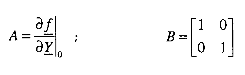
- the now well-known measuring and estimated values, the vehicle parameters (such as vehicle mass m) and the setpoint values used herein as operating points Y 0 are intended ⁇ and ⁇ is to inserted into the already calculated in advance Linearization equations of the vehicle model.
- the system matrix A and the amplification factors are thus obtained and which describe the influence of slip changes on the system behavior.
- the pseudo manipulated variable U ' is calculated from the control deviation X , the feedback matrix F and the feedforward control U Z (see equation (14)).
- the slip values ⁇ should now be calculated in such a way that the desired manipulated variables U 'are realized (see equation 12).
- the slip setpoints are again fed to the slip controller 12, which converts them into brake pressures P i via the brake hydraulics 20.
- control concept described can be used to control the steering angle on the rear wheels in addition to the wheel slip values. To do this, an additional variable ⁇ H must be introduced for the rear wheel steering angle.
- the linearization of the system (10), (11) can also be carried out around other operating points of the state variables Y 0 , for example around the undisturbed natural movement of the system.
- a reference variable feedback matrix W must also be calculated, since the operating point and setpoint do not match.
- the respective actual value of the slip can also be selected.
- optimization can also be simplified if you do not specify slip changes on all wheels. Good control results can already be achieved, for example, if braking is only applied to the front wheel on the outside of the curve and the rear wheel on the inside of the curve. These two wheels help control yaw rate generally much more than the wheels of the other vehicle diagonals.
- the disturbance variables Z (13) can be neglected without the control quality suffering as a result.
- the permissible differences can be constant or increase in a controlled manner after the start of braking.
- Such solutions are already known under the name yaw moment weakening or yaw moment build-up delay. Since the braking forces and the yaw movement are known in the control concept presented here However, depending on the driving condition, more specific permissible braking force differences can be specified.
- phase shifts between the setpoint and actual value are inevitable. This can be taken into account when designing the vehicle controller by including the typical wheel controller dynamics in the model. However, this leads to a higher system order and this can lead to computing time problems.
Abstract
Description
Bei herkömmlichen ABS/ASR-Systemen steht die Längsdynamik des Fahrzeugs im Vordergrund. Stabilität und Beherrschbarkeit des Fahrzeugs werden nicht direkt geregelt, sondern ergeben sich aus invarianten Kompromissen bei der Auslegung des ABS/ASR-Reglers, die nicht in allen Fahrsituationen optimal bezüglich Querdynamik und Bremsweg/Beschleunigung sein können.With conventional ABS / ASR systems, the longitudinal dynamics of the vehicle are in the foreground. The stability and manageability of the vehicle are not regulated directly, but result from invariant compromises in the design of the ABS / ASR controller, which cannot be optimal in all driving situations with regard to lateral dynamics and braking distance / acceleration.
Aus der DE-OS 38 40 456 ist es bekannt, die Beherrschbarkeit eines Fahrzeugs dadurch zu erhöhen, daß die an den Achsen vorhandenen Schräglaufwinkel ermittelt werden und daß hieraus Sollschlupfwerte abgeleitet werden, deren Einhalten die Beherrschbarkeit des Fahrzeugs erhöhen.From DE-OS 38 40 456 it is known to increase the manageability of a vehicle by determining the slip angle present on the axles and from this deriving target slip values, the observance of which increases the manageability of the vehicle.
Gegenüber diesen Stand der Technik wird bei der Erfindung hier ein modellgestützter Reglerentwurf vorgenommen. Das hat den Vorteil, daß die Reglerverstärkungen entsprechend der Fahrsituation und den Fahrbahnverhältnissen ständig neu berechnet werden. Das hier verwendete Zweispurmodell und das Reifenmodell liefern wesentlich bessere Ergebnisse als die sonst oft verwendeten Einspurmodelle. Der Reglerentwurf wird auf der Basis eines Kalman-Filter-Entwurfs durchgeführt und ist damit sehr rechenzeiteffektiv.Compared to this prior art, a model-based controller design is carried out in the invention. This has the advantage that the controller gains are constantly recalculated according to the driving situation and the road conditions. The two-track model and the tire model used here deliver significantly better results than the otherwise often used single-track models. The controller design is based on a Kalman filter design and is therefore very computationally effective.
Außerdem erfolgen die Eingriffe hier gegebenenfalls an allen vier Rädern und die Verteilung auf die Räder erfolgt unter Kraftoptimierungs-Gesichtspunkten. Der Eingriff selbst erfolgt durch Drehung der Kraftrichtungen an den einzelnen Rädern infolge der Schlupfänderungen. Neu ist auch der Einsatz einer Mehrgrößen-Zustandsregelung. Die Zustandsgrößen Schwimmwinkel und Giergeschwindigkeit können innerhalb der physikalischen Grenzen unabhängig voneinander geregelt werden.In addition, the interventions are carried out on all four wheels, if necessary, and the distribution among the wheels takes place from the point of view of power optimization. The intervention itself takes place by rotating the directions of force on the individual wheels as a result of the changes in slip. Another new feature is the use of multivariable state control. The state variables float angle and yaw rate can be controlled independently of one another within the physical limits.
Durch die übergeordnete Fahrdynamikregelung gemäß der Erfindung werden Verbesserungen der Fahrstabilität und der Fahrzeugbeherrschbarkeit bei gleichzeitiger Optimierung der Antriebs-/Bremskraft erzielt.The overriding driving dynamics control according to the invention improves the driving stability and the controllability of the vehicle while at the same time optimizing the drive / braking force.
Dazu wird zunächst ein einfaches, ebenes Modell eines vierrädrigen Straßenfahrzeugs hergeleitet, anhand dessen dann eine Regelung für das Fahrverhalten in allen Fahrzuständen entworfen wird.For this purpose, a simple, flat model of a four-wheel road vehicle is first derived, on the basis of which a regulation for the driving behavior in all driving conditions is then designed.
Das Modell ist von zweiter Ordnung mit den Zustandsgrößen Giergeschwindigkeit ψ̇ und Schwimmwinkel β (s. Fig. 1 und Fig. 2 und Abkürzungsverzeichnis am Beschreibungsende).The model is of the second order with the state variables yaw rate ψ̇ and slip angle β (see Fig. 1 and Fig. 2 and list of abbreviations at the end of the description).
Für den Schwimmwinkel gilt:

(V X Längsgeschwindigkeit, V Y Quergeschwindigkeit)
Damit gilt für die zeitliche Änderung:
Für Relativbewegungen gilt:
![]()
( V X longitudinal speed, V Y transverse speed)
The following applies to the change over time:
The following applies to relative movements:
![]()
Damit lautet die Differentialgleichung für den Schwimmwinkel:
Die Querbeschleunigung a Y läßt sich aus der Summe der an den Reifen quer auf das Fahrzeug wirkenden Kräfte F Y ermitteln (s. Fig. 2).
mit m = Fahrzeugmasse.So the differential equation for the float angle is:
The lateral acceleration a Y can be determined from the sum of the forces F Y acting transversely on the tires on the vehicle (see FIG. 2).
with m = vehicle mass.
An den Vorderrädern müssen zur Ermittlung der Querkräfte bei einem Lenkwinkel δ ungleich Null die Längs- (F B ) und die Seitenkräfte (F S ) an den Reifen berücksichtigt werden.
mit
Die Differentialgleichung für die Giergeschwindigkeit ergibt sich aus den um den Fahrzeugschwerpunkt wirkenden Momenten aus Reifenkräften und den entsprechenden Hebelarmen (s. Fig. 2):
mit
With
The differential equation for the yaw rate results from the moments of tire forces acting around the center of gravity of the vehicle and the corresponding lever arms (see Fig. 2):
With
Damit gilt:
mit
Die Reifenkräfte erhält man bei bekanntem Reifenschlupf und Schräglaufwinkel näherungsweise aus folgender Beziehung:
mit (s. Fig. 3)
Es folgt:
Zwischen dem resultierenden Reifenschlupf S i und dem resultierenden Kraftschlußbeiwert » Ri gibt es einen ähnlichen nichtlinearen Zusammenhang wie zwischen dem bekannten Reifenschlupf λ und dem Kraftschlußbeiwert » in Reifenlängsrichtung. Im folgenden wird davon ausgegangen, daß der Reifen während der ABS-Regelung im allg. den Bereich der Sättigung nicht verläßt, d.h. daß S größer ist als S min (s. Fig. 4). Das kann durch genügend großen Schlupf und/oder durch genügend großen Schräglaufwinkel an den Rädern erreicht werden. Damit wird sichergestellt, daß die zwischen Fahrbahn und Reifen maximal übertragbare Gesamtkraft (aufgeteilt in Längs- und Querkraft) weitgehend ausgenutzt wird.So:
With
With known tire slip and slip angle, the tire forces are obtained approximately from the following relationship:
with (see Fig. 3)
It follows:
There is a similar non-linear relationship between the resulting tire slip S i and the resulting adhesion coefficient » Ri as between the known tire slip λ and the adhesion coefficient» in the longitudinal direction of the tire. In the following it is assumed that the tire generally does not leave the saturation range during the ABS control, ie that S is greater than S min (see FIG. 4). This can be achieved by a sufficiently large slip and / or by a sufficiently large slip angle on the wheels. This ensures that the maximum total force that can be transmitted between the road and the tire (divided into longitudinal and lateral forces) is largely used.
Die Größe der Gesamtkraft F R eines jeden Reifens bleibt im Bereich S>S min annähernd konstant. Durch eine Änderung des Reifenschlupfs bzw. (indirekt über eine Drehung des Fahrzeugs) des Schräglaufwinkels kann jedoch die Richtung der resultierenden Gesamtkraft geändert werden. Auf dieser Änderung der Kraftrichtungen und daraus resultierend der auf das Fahrzeug wirkenden Längs- und Querkräfte und Giermomente beruht die Wirkung des hier beschriebenen Fahrzeugreglers.The size of the total force F R of each tire remains approximately constant in the range S > S min . By changing the tire slip or (indirectly via a rotation of the vehicle) the slip angle, the direction of the resulting total force can be changed. The effect of the vehicle controller described here is based on this change in the force directions and, as a result, on the longitudinal and transverse forces and yaw moments acting on the vehicle.
Die Schräglaufwinkel α i an den Reifen lassen sich wie folgt als Funktion der Zustandsgrößen Schwimmwinkel β und die Giergeschwindigkeit ψ̇ und des Lenkwinkels δ angeben (s. Fig. 5).The slip angle α i on the tires can be specified as a function of the state variables float angle β and the yaw rate ψ̇ and the steering angle δ (see FIG. 5).
Z.B. gilt vorne links:
Da ψ̇·l L klein ist gegenüber V X kann vereinfacht werden zu:
mit
Ebenso kann vorne rechts und hinten verfahren werden.For example, the front left applies:
Since ψ̇ · l L is small compared to V X it can be simplified to:
With
The same can be done at the front right and rear.
Damit gilt für die Schräglaufwinkel:![]()

Aus (1), (2) und (3) und mit (4), (5), (7) und (8) ergeben sich damit folgende Systemgleichungen: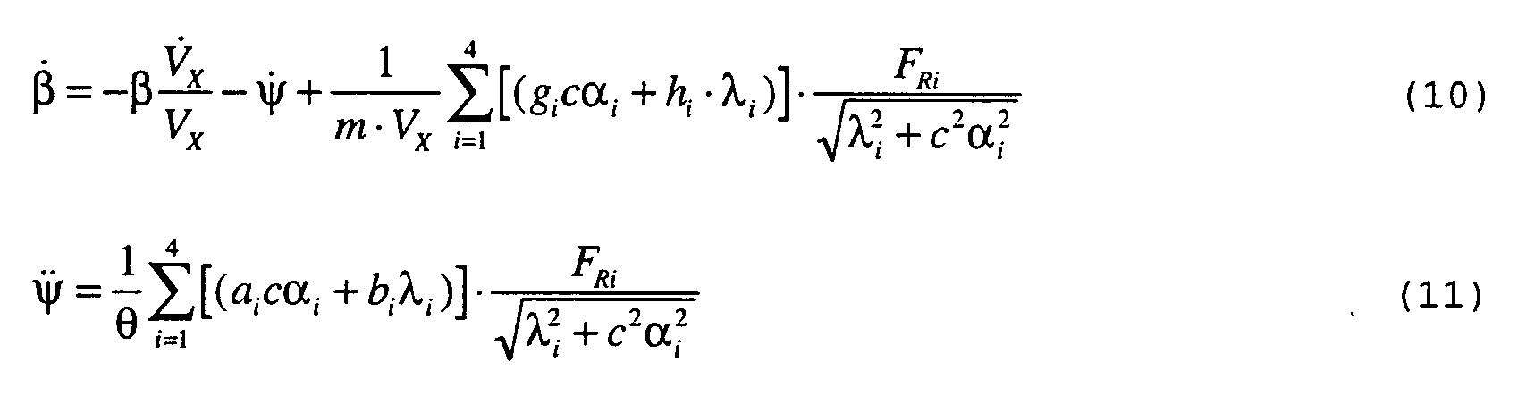
mit (9)![]()
![]()
The following system equations result from (1), (2) and (3) and with (4), (5), (7) and (8):
with (9) ![]()
Der Lenkwinkel kann ebenfalls mit bereits bekannten Einrichtungen gemessen werden.The steering angle can also be measured using already known devices.
Der Schwimmwinkel und die Reifenkräfte können in Verbindung mit einem geeigneten Radschlupf-Regler durch einen Schätzalgorithmus (Beobachter) annähernd bestimmt werden. Ein solcher Beobachter ist in der Patentanmeldung P 40 30 653.4 beschrieben.The float angle and the tire forces can be approximately determined in conjunction with a suitable wheel slip controller using an estimation algorithm (observer). Such an observer is described in patent application P 40 30 653.4.
Fahrzeuglängsgeschwindigkeit und -beschleunigung sind durch die bei ABS/ASR-Einrichtungen vorhandenen Raddrehzahlsensoren und eine entsprechende Auswertung näherungsweise bekannt, ebenso die augenblicklichen Radschlupfwerte an den einzelnen Rädern (Patentanmeldung P 40 24 815.1). Die Schlupfwerte bilden hier die Stellgröße des Reglers, da sie über den Bremsdruck beeinflußt werden können.Longitudinal vehicle speed and acceleration are approximately known from the wheel speed sensors present in ABS / ASR devices and a corresponding evaluation, as are the instantaneous wheel slip values on the individual wheels (patent application P 40 24 815.1). The slip values form the manipulated variable of the controller because they can be influenced via the brake pressure.
Die Parameter Lenkwinkel, Fahrzeuggeschwindigkeit und -beschleunigung und resultierende Reifenkräfte werden als langsam veränderlich und damit quasistationär angenommen.The parameters steering angle, vehicle speed and acceleration and the resulting tire forces are assumed to be slowly changing and thus quasi-stationary.
Für die Fahrzeugparameter Masse, Trägheitsmoment, Schwerpunktslage und Reifensteifigkeiten können geschätzte Werte angenommen werden.Estimated values can be assumed for the vehicle parameters mass, moment of inertia, center of gravity and tire stiffness.
Damit ist das Fahrzeugmodell zweiter Ordnung vollständig bekannt und kann als Grundlage für einen Reglerentwurf verwendet werden.The second-order vehicle model is thus completely known and can be used as the basis for a controller design.
Dazu wird das System zunächst um zeitlich veränderliche Arbeitspunkte linearisiert. Als Arbeitspunkte werden physikalisch realisierbare Werte für den Schwimmwinkel β und die Giergeschwindigkeit ψ̇, z.B. die augenblicklich gewünschten Sollwerte, gewählt.To do this, the system is first linearized around working points that change over time. Physically realizable values for the slip angle β and the yaw rate ψ̇, e.g. the currently desired values.
Nichtlineares System:![]()
![]()
Linearisierung:
Arbeitspunkte der Zustandsgrößen Y (z.B. Solltrajektorie): Y₀(t )
Arbeitspunkte der Stellgrößen λ (z.B. Arbeitspunkt eines unterlagerten Radschlupfreglers, ohne Fahrzeugreglereingriff): λ₀(t )
Der Linearisierungsfehler r wird vernachlässigt.Linearization:
Operating points of the state variables Y (e.g. target trajectory): Y ₀ ( t )
Working points of the manipulated variables λ (e.g. working point of a subordinate wheel slip controller , without intervention by the vehicle controller ): λ₀ ( t )
The linearization error r is neglected.
Für den Reglerentwurf werden zunächst zwei Pseudo-Eingangsgrößen U1' und U2' gebildet.
Die Systemgleichung des linearisierten Systems lautet damit:![]()
Der Term Z wird wie eine Störgröße behandelt, die über die Stellgröße kompensiert werden kann.Two pseudo input variables U 1 'and U 2' are initially formed for the controller design.
The system equation of the linearized system is therefore: ![]()
The term Z is treated like a disturbance variable that can be compensated for via the manipulated variable.
Für den Reglerentwurf werden die Stellgrößen U ' aufgeteilt in die Zustandsgrößenrückführung U und in die Störgrößenaufschaltung U Z .![]()
![]()
![]()
![]()
![]()
![]()
![]()
![]()
Zur Lösung der nichtlinearen Matrix-Riccati-Gleichung stehen dabei bekannte iterative und nichtiterative Verfahren zur Verfügung. Bei den iterativen Verfahren sind die numerischen Schwierigkeiten insbesondere im Hinblick auf einen Echtzeitentwurf nicht zu unterschätzen, nichtiterative Verfahren scheiden von vornherein aufgrund des hohen numerischen Aufwands zur Bestimmung der Eigenwerte und Eigenvektoren des Hamiltonschen kanonischen Systems aus. Es wurde deshalb ein Verfahren zur Bestimmung optimaler Zustandsrückführungen entwickelt, das die oben genannten Schwierigkeiten umgeht. Ausgangspunkt ist das oben aufgeführte System (15).![]()
![]()
![]()
Die Zustandsrückführung wird zu![]()
![]()
![]()
![]()
The status feedback becomes ![]()
Damit gilt:![]()

mit G: Gewichtungsmatrix, diagonal positiv definit.So: ![]()
with G : weighting matrix, diagonally positive defin.
Wählt man![]()

so folgt aus (17):
Führt man den neuen Zustandsvektor![]()
![]()
und aus (18):
mit![]()
Vergleicht man (19) mit der Schätzfehlergleichung eines Beobachters und dem dazughörigen Gütekriterium
so sind bei Wahl von C=1 (19) und (20) formal gleichwertig. Das bedeutet, daß zur Berechnung von F ![]()
![]()
it follows from (17):
If one leads the new state vector ![]()
![]()
and from (18):
With ![]()
If we compare (19) with the estimation error equation of an observer and the associated quality criterion
if C = 1 (19) and (20) are formally equivalent. This means that to calculate F ![]()
Die Gleichungen zur Berechnung von F ![]()

mit
Die Eingangsgröße in Gleichung (15) ergibt sich damit zu:
Bei der Umrechnung der zwei Pseudo-Eingangsgrößen U ' (14) in die vier Stellgrößen Δλ stehen zwei Freiheitsgrade zur Verfügung. Diese können dazu verwendet werden, die Längsverzögerung und damit die Bremskraft in Fahrzeuglängsrichtung zu maximieren, um bei vorgegebenem Fahrzeugverhalten (bezüglich Seiten- und Gierbewegung) einen möglichst kurzen Bremsweg zu erzielen.The equations for calculating F ![]()
With
The input variable in equation (15) thus results in:
Two degrees of freedom are available when converting the two pseudo input variables U '(14) into the four manipulated variables Δλ . These can be used to maximize the longitudinal deceleration and thus the braking force in the longitudinal direction of the vehicle in order to achieve the shortest possible braking distance for a given vehicle behavior (with respect to lateral and yaw movement).
Die Gleichung für die Längsbeschleunigung lautet (s. Fig. 2).
oder mit (3), (7) und (8):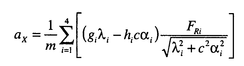
mit![]()
![]()
Als Nebenbedingungen der Minimierungsaufgabe müssen die Gleichungen (12) erfüllt werden:
Außerdem müssen Beschränkungen der Variablen λ i beachtet werden, da der Radbremsschlupf nur Werte zwischen Null und Eins annehmen kann.
Die Sollwerte für den Schwimmwinkel β und für die Giergeschwindigkeit ψ̇ können entsprechend dem gewünschten Fahrverhalten festgelegt werden. Der vom Fahrer durch den Lenkwinkel vorgegebene Wunsch zur Richtungsänderung muß dabei unter Berücksichtigung der Fahrzeuggeschwindigkeit und der Fahrbahnverhältnisse in entsprechende Sollwerte umgerechnet werden.The equation for the longitudinal acceleration is (see Fig. 2).
or with (3), (7) and (8):
With ![]()
![]()
As ancillary conditions for the minimization task, equations (12) must be fulfilled:
In addition, restrictions of the variable λ i must be observed, since the wheel brake slip can only take values between zero and one.
The setpoints for the float angle β and for the yaw rate ψ̇ can be set according to the desired driving behavior. The driver's wish for a change of direction, as determined by the steering angle, must be converted into corresponding target values, taking into account the vehicle speed and the road conditions.
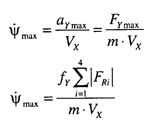
Sollwert für ψ̇:
V Ch ist dabei eine Konstante, die das Fahrverhalten bei höheren Geschwindigkeiten beeinflußt. Dieser Rohwert muß bei großem Lenkwinkel, hoher Fahrzeuggeschwindigkeit oder niedrigem Haftreibbeiwert der Fahrbahn auf einen sinnvollen Wert begrenzt werden, da sonst die Giergeschwindigkeit größer wird als die maximal mögliche Winkeländerungsgeschwindigkeit der Bahnkurve. Dann nimmt der Schwimmwinkel zu und das Fahrzeug schleudert.Setpoint for ψ̇:
V Ch is a constant that influences driving behavior at higher speeds. With a large steering angle, high vehicle speed or low coefficient of static friction on the road, this raw value must be limited to a reasonable value, since otherwise the yaw rate will be greater than the maximum possible angular rate of change of the path curve. Then the float angle increases and the vehicle skids.
Um das zu vermeiden wird z.B. festgelegt, welchen Anteil der maximal verfügbaren Gesamtkraft die Querkraft in Anspruch nehmen darf.
mit![]()

Für den Schwimmwinkel können neben echten Sollwerten auch Begrenzungen vorgegeben werden, die verhindern, daß der Schwimmwinkel zu groß wird. Eine Regelabweichung der ersten Zustandsgröße ergibt sich in diesem Fall nur, wenn der Betrag des Schwimmwinkels seine Begrenzung überschreitet. Die Begrenzung kann z.B. so festgelegt werden, daß bei Bremsschlupf Null der resultierende Schlupf S an den Hinterrädern die Sättigungsgrenze S min nicht wesentlich überschreitet (s. Fig. 4, (6)).To avoid this, it is determined, for example, what proportion of the maximum available total force the shear force may use.
With ![]()
In addition to real setpoints, limits can also be specified for the float angle, which prevent the float angle from becoming too large. In this case, there is a control deviation of the first state variable only if the amount of the float angle exceeds its limit. The limitation can be determined, for example, so that when the brake slip is zero, the resulting slip S on the rear wheels does not significantly exceed the saturation limit S min (see FIG. 4, (6)).
Der oben beschriebene Fahrzeugregler kann mit einem Algorithmus zur Schätzung der Fahrzeugouergeschwindigkeit und der Reifenkräfte (P 40 30 653.4, Anlage I) und mit einem anderen Algorithmus zur Einstellung der vom Fahrzeugregler vorgegebenen Sollschlupfwerte an den einzelnen Rädern (z.B. Patentanmeldung P 40 30 724.7 Anlage III, und P 40 24 815.1, Anlage II) kombiniert werden. Fig. 6 zeigt eine Übersicht des Gesamtsystems bei ABS.The vehicle controller described above can be used with an algorithm for estimating the vehicle speed and the tire forces (P 40 30 653.4, Appendix I) and with another algorithm for setting the target slip values on the individual wheels specified by the vehicle controller (e.g. patent application P 40 30 724.7 Appendix III, and P 40 24 815.1, Appendix II) can be combined. 6 shows an overview of the overall system in ABS.
Auf das Fahrzeug 1 wirkt von außen der Lenkwinkel δ und der Kraftschlußbeiwert »₀ ein. Am Fahrzeug 1 werden die Radgeschwindigkeiten V Ri , der Lenkwinkel δ und die Giergeschwindigkeit ψ̇ gemessen, außerdem eventuell der Vordruck P der Bremsanlage oder die einzelnen Radbremszylinderdrücke P i . Bei ASR-Reglern werden außerdem z.B. die Motordrehzahl und der Drosselklappenwinkel gemessen. Ein Schlupfregler 2 schätzt daraus unter Zuhilfenahme der von einem Beobachter 3 gelieferten Größen die Bremskräfte F̂ B und die Fahrzeuglängsgeschwindigkeit V̂ X und -beschleunigung ![]()
![]()
Fig. 7 zeigt als Beispiel einen groben Ablaufplan des Verfahrens.7 shows a rough flowchart of the method as an example.
Dieses Verfahren kann in eine Programmiersprache umgesetzt und auf einem geeigneten Digitalrechner (Mikroprozessor) implementiert werden. Es bietet gegenüber herkömmlichen ABS/ASR-Systemen eine erhöhte Fahrzeugstabilität (sicheres Verhindern von Schleudervorgängen), eine verbesserte Lenkbarkeit mit durch die Sollwerte vorgebbarem Lenkverhalten und bei Lenkmanövern eine bessere Ausnutzung des Kraftschlußpotentials der Fahrbahn und damit einen kürzeren Bremsweg bzw. eine bessere Fahrzeugbeschleunigung. Die bei herkömmlichen Systemen notwendigen Kompromisse zur Beherrschung aller vorkommenden Fahr- und Straßensituationen entfallen weitgehend.This method can be implemented in a programming language and implemented on a suitable digital computer (microprocessor). Compared to conventional ABS / ASR systems, it offers increased vehicle stability (safe prevention of skidding), improved steerability with steering behavior that can be specified by the setpoints, and better steering potential utilization of the road surface during steering maneuvers and thus a shorter braking distance or better vehicle acceleration. The compromises necessary with conventional systems to master all driving and road situations that occur are largely eliminated.
Das hier beschriebene Regelungskonzept kann in allen Fahrsituationen eingesetzt werden, nicht nur bei ABS/ASR-Betieb.The control concept described here can be used in all driving situations, not only in ABS / ASR operation.
Block 10 stellt das Fahrzeug dar. An ihm werden mit einem Block 11 Meßtechnik die Radgeschwindigkeiten V Ri , die Giergeschwindigkeit ψ̇ der Lenkwinkel δ und der Vordruck P oder die Radbremsdrücke P i gemessen. In einem schlupfregler 12 werden hieraus die Größen Längsgeschwindigkeit V̂ X , Längsbeschleunigung![]()
![]()
In Block 16 werden die nun bekannten Meß- und Schätzwerte, die Fahrzeugparameter (z.B. Fahrzeugmasse m) und die hier als Arbeitspunkte Y₀ verwendeten Sollwerte β soll und ψ̇ soll in die bereits im voraus berechneten Linearisierungsgleichungen des Fahrzeugmodells eingesetzt. Man erhält damit die Systemmatrix A und die Verstärkungsfaktoren![]()
und![]()
welche den Einfluß von Schlupfänderungen auf das Systemverhalten beschreiben.In ![]()
and ![]()
which describe the influence of slip changes on the system behavior.
Im Block 17 kann für das nunmehr bekannte, linearisierte System (s. Gleichung (15)) wie beschrieben ein Reglerentwurf durchgeführt werden und man erhält die Zustandsgrößenrückführmatrix F.In
In Block 18 wird aus der Regelabweichung X , der Rückführmatrix F und der Störgrößenaufschaltung U Z die Pseudo-Stellgröße U' berechnet (s. Gleichung (14)). Nach der beschriebenen Methode der Längskraftoptimierung werden nun die Schlupfwerte λ soll so berechnet, daß die gewünschten Stellgrößen U' realisiert werden (s. Gleichung 12)).In
Die Schlupfsollwerte werden wieder dem Schlupfregler 12 zugeführt, der sie über die Bremshydraulik 20 in Bremsdrücke P i umsetzt.The slip setpoints are again fed to the
Das bisher beschriebene Fahrzeugregelungskonzept kann bei Bedarf verändert beziehungsweise erweitert werden.The vehicle control concept described so far can be changed or expanded if necessary.
Bei entsprechender Ausrüstung des Fahrzeugs kann mit dem beschriebenen Regelkonzept zusätzlich zu den Radschlupfwerten auch der Lenkwinkel an den Hinterrädern geregelt werden. Dazu muß eine zusätzliche Größe δ H für den Hinterradlenkwinkel eingeführt werden.If the vehicle is equipped accordingly, the control concept described can be used to control the steering angle on the rear wheels in addition to the wheel slip values. To do this, an additional variable δ H must be introduced for the rear wheel steering angle.
Nach einer Linearisierung von δ H um δ H =0 lautet die Gleichung für die Querbeschleunigung (2):
mit![]()

Die Gleichung (4) für die Gierbeschleunigung lautet nun: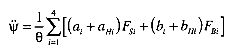
Die Definitionen (5) werden ergänzt durch:
Die Gleichung (8) für die Schräglaufwinkel lautet nach Einführung des Hinterradwinkels:![]()

Die Linearisierung des Systems![]()
![]()
With ![]()
The equation (4) for yaw acceleration is now:
The definitions (5) are supplemented by:
The equation (8) for the slip angle is after the introduction of the rear wheel angle: ![]()
The linearization of the system ![]()
![]()
Die Gleichungen (12) für die Pseudo-Eingangsgrößen lauten dann: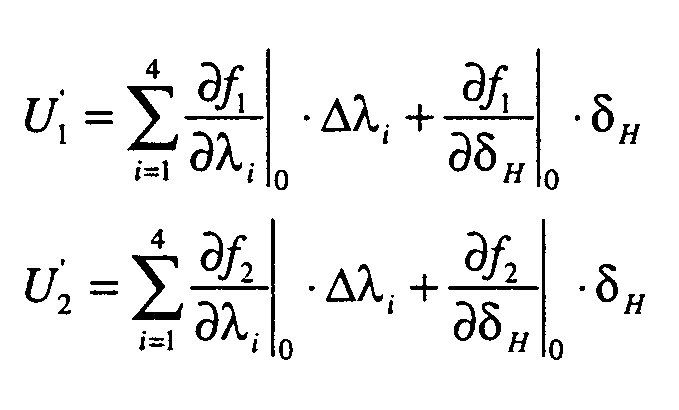
Für die Bremskraftoptimierung steht damit ein zusätzlicher, dritter Freiheitsgrad zur Verfügung.The equations (12) for the pseudo input variables are then:
An additional, third degree of freedom is therefore available for brake force optimization.
Die Linearisierung des Systems (10), (11) kann außer um die Solltrajektorie auch um andere Arbeitspunkte der Zustandsgrößen Y₀ durchgeführt werden, z.B. um die ungestörte Eigenbewegung des Systems. In diesem Fall muß außer der Zustandsgrößenrückführmatrix F auch noch eine Führungsgrößenrückführmatrix W berechnet werden, da Arbeitspunkt und Sollwert nicht übereinstimmen. Als Arbeitspunkt für die Stellgrößen λ₀ kann z.B. auch der jeweilige Istwert des Schlupfs gewählt werden.In addition to the target trajectory, the linearization of the system (10), (11) can also be carried out around other operating points of the state variables Y ₀ , for example around the undisturbed natural movement of the system. In this case, in addition to the state variable feedback matrix F , a reference variable feedback matrix W must also be calculated, since the operating point and setpoint do not match. As a working point for the manipulated variables λ₀ , for example, the respective actual value of the slip can also be selected.
Neben dem Riccati-Entwurf und dem oben beschriebenen Reglerentwurf über Kalman-Filter kann auch ein anderes Reglerentwurfsverfahren verwendet werden, z.B. mit Hilfe einer Polvorgabe.In addition to the Riccati design and the controller design described above using Kalman filters, another controller design process can also be used, e.g. with the help of a pole specification.
Für die oben beschriebene Bremskraftoptimierung gibt es auch weniger rechenzeitintensive Alternativen, die zu nur wenig schlechteren Resultaten führen. Beispielsweise kann an den Vorder- bzw. Hinterrädern links und rechts jeweils derselbe Sollschlupfwert vorgegeben werden. Bei annähernd gleichen Schräglaufwinkeln links und rechts ist nach Gleichung (7) auch das Verhältnis von Seiten- zu Bremskraft und damit die Richtung der resultierenden Kraft F Ri links und rechts jeweils fast gleich. Die dabei erzielte Längsverzögerung liegt nur unwesentlich unter der durch die vollständige Optimierung erreichbaren. Die Optimierung entfällt, weil durch die zwei Zwangsbedingungen![]()
![]()
![]()
![]()
Die Optimierung kann auch vereinfacht werden, wenn darauf verzichtet wird, an allen Rädern Schlupfänderungen vorzugeben. Gute Regelungsergebnisse können z.B. bereits erzielt werden, wenn bei Kurvenbremsungen jeweils nur am kurienäußeren Vorderrad und am kurveninneren Hinterrad eingegriffen wird. Diese zwei Räder tragen zur Steuerung der Giergeschwindigkeit im allgemeinen wesentlich mehr bei, als die Räder der anderen Fahrzeugdiagonalen.Optimization can also be simplified if you do not specify slip changes on all wheels. Good control results can already be achieved, for example, if braking is only applied to the front wheel on the outside of the curve and the rear wheel on the inside of the curve. These two wheels help control yaw rate generally much more than the wheels of the other vehicle diagonals.
Für die Optimierung der Fahrzeugbeschleunigung gilt entsprechendes. In vielen Fällen ist es möglich, auf die Eingangsgröße U'₁ ganz zu verzichten. Die Eingangsmatrix lautet dann:
Dies muß beim Reglerentwurf berücksichtigt werden. Auch mit nur einer Stellgröße ist das System vollständig steuerbar. Zur Bremskraftoptimierung muß nur die zweite Gleichung in (12) berücksichtigt werden.The same applies to the optimization of vehicle acceleration. In many cases it is possible to dispense with the input variable U'₁ entirely. The input matrix is then:
This must be taken into account when designing the controller. The system can be fully controlled even with just one manipulated variable. To optimize braking force, only the second equation in (12) has to be taken into account.
Wenn die Modellparameter ohnehin nicht genau genug bekannt sind, können die Störgrößen Z (13) vernachlässigt werden, ohne daß darunter die Regelgüte leidet.If the model parameters are not known well enough anyway, the disturbance variables Z (13) can be neglected without the control quality suffering as a result.
In Sonderfällen, wie stark unterschiedlichen Haftreibbeiwerten der Fahrbahn unter den Rädern links und rechts können zusätzliche Maßnahmen zur Erzielung eines zufriedenstellenden Fahrverhaltens erforderlich sein. Das oben beschriebene Regelungskonzept, bei dem der Bereich der Reifensättigung nicht verlassen werden darf (s. Fig. 4) kann in solchen Fällen zu einer zu starken Gierbewegung und damit zu Fahrzeuginstabilität führen. Verbesserungen lassen sich durch eine Begrenzung der Druckdifferenzen bzw. der Bremskraftdifferenzen an den Hinterrädern erreichen.In special cases, such as very different static friction coefficients of the road under the left and right wheels, additional measures may be necessary to achieve satisfactory driving behavior. The control concept described above, in which the area of tire saturation must not be left (see FIG. 4), can in such cases lead to excessive yaw movement and thus to vehicle instability. Improvements can be achieved by limiting the pressure differences or the braking force differences on the rear wheels.
Die zulässigen Differenzen können konstant sein oder nach Bremsbeginn gesteuert ansteigen. Solche Lösungen sind bereits unter dem Namen Giermomentabschwächung bzw. Giermomentaufbauverzögerung bekannt. Da beim hier vorgestellten Regelkonzept die Bremskräfte und die Gierbewegung bekannt sind, können jedoch je nach Fahrzustand gezielter zulässige Bremskraftdifferenzen vorgegeben werden.The permissible differences can be constant or increase in a controlled manner after the start of braking. Such solutions are already known under the name yaw moment weakening or yaw moment build-up delay. Since the braking forces and the yaw movement are known in the control concept presented here However, depending on the driving condition, more specific permissible braking force differences can be specified.
Wenn ein unterlagerter Radregler zur Einstellung der vorgegebenen Schlupfwerte benötigt wird, sind Phasenverschiebungen zwischen Soll- und Istwert unvermeidlich. Dies kann beim Entwurf des Fahrzeugreglers durch eine Einbeziehung der typischen Radreglerdynamik in das Modell berücksichtigt werden. Dies führt jedoch zu einer höheren Systemordnung und es kann dadurch zu Rechenzeitproblemen kommen. Alternativ dazu kann die Phasenverschiebung des unterlagerten Reglers näherungsweise durch die Einführung eines D-Anteils in der Rückführung der Zustandsgrößen kompensiert werden. Der Regelsatz lautet dann:![]()
![]()
a X , a Y - Längs-/Querbeschleunigung im Fahrzeugschwerpunkt
C λ, C α - Längs-/Seitensteifigkeit des Reifens
F Bi , F Si - Reifenkräfte in Reifenlängs-/querrichtung
F Xi , F Yi - Reifenkräfte in Fahrzeuglängs-/querrichtung
F Zi - Aufstandskraft des Reifens
m - Fahrzeugmasse
S i - Resultierender Reifenschlupf
V X , V Y - Fahrzeuglängs-/quergeschwindigkeit im Schwerpunkt
V̇ X , V̇ Y - Zeitliche Änderung der Längs-/quergeschwindigkeit
V Xi , V Yi - Fahrzeuglängs-/quergeschwindigkeit am Rad
V Ch - Charakterische Geschwindigkeit V Ch - Charakterische Geschwindigkeit
α i - Schräglaufwinkel des Rades
β - Schwimmwinkel des Fahrzeugs im Schwerpunkt
δ - Lenkwinkel (vorne)
δ H - Lenkwinkel an den Hinterrädern
ψ̇ - Gierwinkelgeschwindigkeit
λ i - Reifenschlupf
» Ri - Resultierender Kraftschlußbeiwert
ϑ - Trägheitsmoment um Fahrzeughochachse
l V , l H , l L , l R - geometrische Abmessungen (Schwerpunktslage)
A, B, ... - Matrizen
a , b , X ... - Vektoren
λ![]()
V Ri - Radgeschwindigkeit
P - Vordruck
P i - Radbremsdruck
F R - Gesamtkraft des Reifens
a X , a Y - longitudinal / lateral acceleration in the center of gravity
C λ , C α - longitudinal / lateral stiffness of the tire
F Bi , F Si - tire forces in the longitudinal / transverse direction of the tire
F Xi , F Yi - tire forces in the vehicle's longitudinal / transverse direction
F Zi - tire contact force
m - vehicle mass
S i - Resulting tire slip
V X , V Y - vehicle longitudinal / lateral speed in the center of gravity
V̇ X , V̇ Y - change over time in the longitudinal / transverse speed
V Xi , V Yi - vehicle longitudinal / lateral speed on the wheel
V Ch - Characteristic speed V Ch - Characteristic speed
α i - slip angle of the wheel
β - the vehicle's swimming angle in the center of gravity
δ - steering angle (front)
δ H - steering angle on the rear wheels
ψ̇ - yaw rate
λ i - tire slip
» Ri - Resulting adhesion coefficient
ϑ - moment of inertia around vehicle vertical axis
l V , l H , l L , l R - geometric dimensions (center of gravity)
A , B , ... - Matrices
a , b , X ... - vectors
λ ![]()
V Ri - wheel speed
P - form
P i - wheel brake pressure
F R - total force of the tire
Claims (2)
- Method for improving the controllability of motor vehicles, desired slip values λbeing determined for the individual wheels with the aid of the measured variable of yaw rate ψ̇ and the longitudinal speed V X determined and the wheel slips being adjusted accordingly at at least some of the wheels by means of an antiblock control system or drive slip control system, characterised in that, in addition to the measurement variable of yaw rate ψ̇, the wheel speeds V Ri , the steering angle δ, the inlet pressure P or the wheel brake cylinder pressure P i and, in a drive slip control system, the engine speed and the throttle valve angle are measured, in that the longitudinal vehicle speed V̂ X , the longitudinal vehicle acceleration
 X , the wheel slip values λ i and the tyre forces in the tyre longitudinal direction F̂ Bi are estimated herefrom, in that these variables V̂ X ,
 X and λ i are fed to a vehicle controller and the variables V̂ X , λ i and F̂ Bi are fed to an observer for estimating the total force F̂ R and the transverse speed V̂ Y , which observer then passes the latter on to the vehicle controller, and in that desired slip values λ
 at the wheels are determined in the vehicle controller with the aid of a simple model, and are adjusted using an antiblock control system or drive slip control system.
- Method according to Claim 1, characterised in that the desired slip values are fed to an antiblock/drive slip control system, which for its part gererates desired slip values, and in that the deviation of one desired slip value from the other is superimposed thereupon.
Applications Claiming Priority (3)
| Application Number | Priority Date | Filing Date | Title |
|---|---|---|---|
| DE4030704 | 1990-09-28 | ||
| DE4030704A DE4030704C2 (en) | 1990-09-28 | 1990-09-28 | Method for improving the controllability of motor vehicles when braking |
| PCT/EP1991/001837 WO1992005984A2 (en) | 1990-09-28 | 1991-09-26 | Method of improving vehicle control when braking |
Publications (2)
| Publication Number | Publication Date |
|---|---|
| EP0503030A1 EP0503030A1 (en) | 1992-09-16 |
| EP0503030B1 true EP0503030B1 (en) | 1995-12-06 |
Family
ID=6415169
Family Applications (1)
| Application Number | Title | Priority Date | Filing Date |
|---|---|---|---|
| EP91916870A Expired - Lifetime EP0503030B1 (en) | 1990-09-28 | 1991-09-26 | Method of improving vehicle control when braking |
Country Status (6)
| Country | Link |
|---|---|
| EP (1) | EP0503030B1 (en) |
| JP (2) | JPH05502422A (en) |
| KR (1) | KR100215611B1 (en) |
| AT (1) | ATE131119T1 (en) |
| DE (2) | DE4030704C2 (en) |
| WO (1) | WO1992005984A2 (en) |
Families Citing this family (43)
| Publication number | Priority date | Publication date | Assignee | Title |
|---|---|---|---|---|
| DE4030724B4 (en) * | 1990-09-28 | 2005-05-04 | Robert Bosch Gmbh | Anti-lock control system |
| JPH04292250A (en) * | 1991-03-20 | 1992-10-16 | Hitachi Ltd | Antiskid controller and method thereof |
| DE4217710A1 (en) * | 1992-06-01 | 1993-12-02 | Porsche Ag | Continuous detection of slippery winter road surfaces - determining and comparing driving parameters and boundary conditions for motor car |
| DE4225983C2 (en) * | 1992-08-06 | 2002-03-14 | Bosch Gmbh Robert | Method for braking vehicle wheels |
| DE4229504B4 (en) * | 1992-09-04 | 2007-11-29 | Robert Bosch Gmbh | Method for regulating vehicle stability |
| DE4243717A1 (en) * | 1992-12-23 | 1994-06-30 | Bosch Gmbh Robert | Procedure for regulating vehicle stability |
| JP3150832B2 (en) * | 1993-10-26 | 2001-03-26 | トヨタ自動車株式会社 | Vehicle braking control device |
| DE4419131B4 (en) * | 1993-06-11 | 2008-12-18 | Volkswagen Ag | Motor vehicle, preferably passenger car |
| DE4340932B4 (en) * | 1993-12-01 | 2005-08-25 | Robert Bosch Gmbh | Method for regulating the driving stability of a motor vehicle |
| DE4418772C2 (en) * | 1994-05-28 | 2000-08-24 | Daimler Chrysler Ag | Method for regulating the brake pressure as a function of the deviation of the actual wheel slip from a target slip |
| US5671143A (en) * | 1994-11-25 | 1997-09-23 | Itt Automotive Europe Gmbh | Driving stability controller with coefficient of friction dependent limitation of the reference yaw rate |
| US5774821A (en) | 1994-11-25 | 1998-06-30 | Itt Automotive Europe Gmbh | System for driving stability control |
| US5742507A (en) | 1994-11-25 | 1998-04-21 | Itt Automotive Europe Gmbh | Driving stability control circuit with speed-dependent change of the vehicle model |
| US5710704A (en) | 1994-11-25 | 1998-01-20 | Itt Automotive Europe Gmbh | System for driving stability control during travel through a curve |
| US5735584A (en) * | 1994-11-25 | 1998-04-07 | Itt Automotive Europe Gmbh | Process for driving stability control with control via pressure gradients |
| US5711024A (en) | 1994-11-25 | 1998-01-20 | Itt Automotive Europe Gmbh | System for controlling yaw moment based on an estimated coefficient of friction |
| US5694321A (en) | 1994-11-25 | 1997-12-02 | Itt Automotive Europe Gmbh | System for integrated driving stability control |
| DE19515053A1 (en) * | 1994-11-25 | 1996-05-30 | Teves Gmbh Alfred | Regulating travel stability of vehicle using desired value |
| US5701248A (en) | 1994-11-25 | 1997-12-23 | Itt Automotive Europe Gmbh | Process for controlling the driving stability with the king pin inclination difference as the controlled variable |
| JP3724845B2 (en) * | 1995-06-09 | 2005-12-07 | 本田技研工業株式会社 | Anti-lock brake control method for vehicle |
| JP3348567B2 (en) * | 1995-07-20 | 2002-11-20 | トヨタ自動車株式会社 | Vehicle braking control device |
| JPH09156487A (en) * | 1995-12-13 | 1997-06-17 | Fuji Heavy Ind Ltd | Braking force control device |
| DE19707106B4 (en) * | 1996-03-30 | 2008-12-04 | Robert Bosch Gmbh | System for controlling brake systems |
| DE19617590A1 (en) * | 1996-05-02 | 1997-11-06 | Teves Gmbh Alfred | Method for determining a target vehicle behavior |
| DE19749005A1 (en) * | 1997-06-30 | 1999-01-07 | Bosch Gmbh Robert | Method and device for regulating movement variables representing vehicle movement |
| DE19820107A1 (en) * | 1997-12-20 | 1999-06-24 | Itt Mfg Enterprises Inc | Method of improving driving quality of a vehicle with brakes applied while cornering |
| DE19812238A1 (en) * | 1998-03-20 | 1999-09-23 | Daimler Chrysler Ag | Procedure for controlling the yaw behavior of vehicles |
| JP3458734B2 (en) | 1998-04-09 | 2003-10-20 | トヨタ自動車株式会社 | Vehicle motion control device |
| DE19851978A1 (en) * | 1998-11-11 | 2000-05-25 | Daimler Chrysler Ag | Procedure for controlling the lateral dynamics of a vehicle with front axle steering |
| JP3621842B2 (en) | 1999-02-01 | 2005-02-16 | トヨタ自動車株式会社 | Vehicle motion control device |
| DE19954198B4 (en) * | 1999-02-11 | 2011-08-18 | Continental Teves AG & Co. OHG, 60488 | Method and device for determining a braking force acting in the footprint of a wheel of a vehicle |
| DE10209884B4 (en) * | 2001-03-09 | 2018-10-25 | Continental Teves Ag & Co. Ohg | Vehicle stabilizing device |
| DE10254392A1 (en) * | 2002-11-18 | 2004-05-27 | Volkswagen Ag | Regulating vehicle dynamics involves detecting variable system parameter deviation from base value, identifying system parameter, determining identified system model, adapting control gain to model |
| DE10355701A1 (en) * | 2003-11-28 | 2005-06-16 | Zf Friedrichshafen Ag | Method for controlling and regulating the driving dynamics of a vehicle |
| JP4720107B2 (en) | 2004-05-27 | 2011-07-13 | 日産自動車株式会社 | Driver model and vehicle function control system assist function evaluation device equipped with the model |
| DE102004034067A1 (en) * | 2004-07-15 | 2006-02-09 | Bayerische Motoren Werke Ag | Method for stabilizing vehicle during braking operation on inclined surface, comprising shifting of activation point of torque regulating device |
| DE102004035004A1 (en) * | 2004-07-20 | 2006-02-16 | Bayerische Motoren Werke Ag | Method for increasing the driving stability of a motor vehicle |
| DE102005011831B4 (en) * | 2005-03-15 | 2011-12-08 | Audi Ag | Method for determining a setpoint slip specification in an antilock braking system of a vehicle |
| WO2007074714A1 (en) * | 2005-12-27 | 2007-07-05 | Honda Motor Co., Ltd. | Controller of vehicle |
| EP1967433B1 (en) * | 2005-12-27 | 2010-09-29 | Honda Motor Co., Ltd. | Vehicle control device |
| DE102006009682A1 (en) * | 2006-03-02 | 2007-09-06 | Bayerische Motoren Werke Ag | Dual-tracked vehicle`s driving condition determining method, involves using tire or wheel forces in vehicle-transverse direction, direction of vehicle-vertical axis and direction of longitudinal direction as value measured at vehicle |
| DE102008036545B4 (en) * | 2008-07-16 | 2023-06-01 | Continental Automotive Technologies GmbH | Method for improving motor vehicle ABS control |
| US8977430B2 (en) | 2012-12-26 | 2015-03-10 | Robert Bosch Gmbh | Electronic stability control system indicator |
Family Cites Families (13)
| Publication number | Priority date | Publication date | Assignee | Title |
|---|---|---|---|---|
| JPS61500724A (en) * | 1983-12-16 | 1986-04-17 | ロ−ベルト ボツシユ ゲゼルシヤフト ミツト ベシユレンクテル ハフツング | How to determine the optimal slip value |
| JPH0613287B2 (en) * | 1984-05-21 | 1994-02-23 | 日産自動車株式会社 | Vehicle braking force control device |
| DE3535843A1 (en) * | 1985-10-08 | 1987-04-16 | Bosch Gmbh Robert | METHOD FOR CONTINUOUSLY DETERMINING THE FACTORY VALUE (MY) |
| DE3826982C2 (en) * | 1987-08-10 | 2000-11-30 | Denso Corp | Auxiliary steering system connected to an anti-lock control system for use in motor vehicles |
| DE3731756A1 (en) * | 1987-09-22 | 1989-03-30 | Bosch Gmbh Robert | METHOD FOR REGULATING THE DRIVING STABILITY OF A VEHICLE |
| US4882693A (en) * | 1987-12-28 | 1989-11-21 | Ford Motor Company | Automotive system for dynamically determining road adhesion |
| JP2804760B2 (en) * | 1988-01-22 | 1998-09-30 | 雅彦 三成 | Car operation control device |
| DE3819474C1 (en) * | 1988-06-08 | 1989-11-30 | Daimler-Benz Aktiengesellschaft, 7000 Stuttgart, De | |
| DE3825639C2 (en) * | 1988-07-28 | 1995-10-12 | Sepp Gunther | Device for stabilizing motor vehicles when cornering |
| DE3840456A1 (en) * | 1988-12-01 | 1990-06-07 | Bosch Gmbh Robert | METHOD FOR INCREASING THE CONTROL OF A VEHICLE |
| DE3905045A1 (en) * | 1989-02-18 | 1990-08-23 | Teves Gmbh Alfred | CIRCUIT ARRANGEMENT FOR A BRAKE SYSTEM WITH ANTI-BLOCKING PROTECTION AND / OR DRIVE SLIP CONTROL |
| DE3912045A1 (en) * | 1989-04-12 | 1990-10-25 | Bayerische Motoren Werke Ag | METHOD FOR REGULATING A CROSS-DYNAMIC STATE SIZE OF A MOTOR VEHICLE |
| DE3933652A1 (en) * | 1989-10-09 | 1991-04-11 | Bosch Gmbh Robert | ANTI-BLOCKING CONTROL SYSTEM AND DRIVE-SLIP CONTROL SYSTEM |
-
1990
- 1990-09-28 DE DE4030704A patent/DE4030704C2/en not_active Expired - Lifetime
-
1991
- 1991-09-26 WO PCT/EP1991/001837 patent/WO1992005984A2/en active IP Right Grant
- 1991-09-26 KR KR1019920701277A patent/KR100215611B1/en not_active IP Right Cessation
- 1991-09-26 EP EP91916870A patent/EP0503030B1/en not_active Expired - Lifetime
- 1991-09-26 DE DE59107033T patent/DE59107033D1/en not_active Expired - Lifetime
- 1991-09-26 AT AT91916870T patent/ATE131119T1/en not_active IP Right Cessation
- 1991-09-26 JP JP3515246A patent/JPH05502422A/en active Pending
-
2002
- 2002-09-04 JP JP2002258598A patent/JP2003127850A/en active Pending
Also Published As
| Publication number | Publication date |
|---|---|
| KR920702305A (en) | 1992-09-03 |
| DE59107033D1 (en) | 1996-01-18 |
| ATE131119T1 (en) | 1995-12-15 |
| KR100215611B1 (en) | 1999-08-16 |
| DE4030704A1 (en) | 1992-04-02 |
| JPH05502422A (en) | 1993-04-28 |
| WO1992005984A2 (en) | 1992-04-16 |
| JP2003127850A (en) | 2003-05-08 |
| EP0503030A1 (en) | 1992-09-16 |
| WO1992005984A3 (en) | 1992-05-14 |
| DE4030704C2 (en) | 2000-01-13 |
Similar Documents
| Publication | Publication Date | Title |
|---|---|---|
| EP0503030B1 (en) | Method of improving vehicle control when braking | |
| EP1682392B1 (en) | Method and system for improving the handling characteristics of a vehicle | |
| EP0943515B1 (en) | Method for controlling of the yaw-behavior of vehicles | |
| EP0625946B1 (en) | Method of controlling vehicle stability | |
| EP1768888B1 (en) | Method for increasing the driving stability of a motor vehicle | |
| EP1807300B1 (en) | Method and device for assisting a motor vehicle server for the vehicle stabilisation | |
| EP0943514B1 (en) | Process and device for the drive-dynamism-regulation on a road-vehicle | |
| DE19515056A1 (en) | Motor vehicle individual wheel braking system preserving steerability of vehicle | |
| DE10016343A1 (en) | Dynamic vehicle control device has rear wheel steering angle control stage that aligns rear wheel steering angle command value in line with actual steering angle setting | |
| WO2005063538A1 (en) | Method for regulating a brake pressure in case of non-homogeneous coefficients of friction of a roadway | |
| DE112013006766T5 (en) | A method for calculating a target movement state amount of a vehicle | |
| DE102006033635A1 (en) | Process to stabilize the track of a moving automobile using driver inputs and correction for lateral disturbance | |
| EP0829401A2 (en) | Procedure and device for controlling the lateral dynamic attitude of a vehicle | |
| DE10329278A1 (en) | Stabilizer, vehicle equipped with it and stabilization method | |
| DE10103629A1 (en) | Method for controlling the driving stability of a vehicle | |
| WO2001083277A1 (en) | Method for controlling the handling stability of a vehicle |
Legal Events
| Date | Code | Title | Description |
|---|---|---|---|
| PUAI | Public reference made under article 153(3) epc to a published international application that has entered the european phase |
Free format text: ORIGINAL CODE: 0009012 |
|
| 17P | Request for examination filed |
Effective date: 19920514 |
|
| AK | Designated contracting states |
Kind code of ref document: A1 Designated state(s): AT DE FR GB IT SE |
|
| 17Q | First examination report despatched |
Effective date: 19941013 |
|
| GRAA | (expected) grant |
Free format text: ORIGINAL CODE: 0009210 |
|
| AK | Designated contracting states |
Kind code of ref document: B1 Designated state(s): AT DE FR GB IT SE |
|
| REF | Corresponds to: |
Ref document number: 131119 Country of ref document: AT Date of ref document: 19951215 Kind code of ref document: T |
|
| REF | Corresponds to: |
Ref document number: 59107033 Country of ref document: DE Date of ref document: 19960118 |
|
| ET | Fr: translation filed | ||
| ITF | It: translation for a ep patent filed |
Owner name: STUDIO JAUMANN |
|
| PG25 | Lapsed in a contracting state [announced via postgrant information from national office to epo] |
Ref country code: SE Effective date: 19960306 |
|
| GBT | Gb: translation of ep patent filed (gb section 77(6)(a)/1977) |
Effective date: 19960221 |
|
| PLBE | No opposition filed within time limit |
Free format text: ORIGINAL CODE: 0009261 |
|
| STAA | Information on the status of an ep patent application or granted ep patent |
Free format text: STATUS: NO OPPOSITION FILED WITHIN TIME LIMIT |
|
| 26N | No opposition filed | ||
| PG25 | Lapsed in a contracting state [announced via postgrant information from national office to epo] |
Ref country code: FR Effective date: 19970630 |
|
| REG | Reference to a national code |
Ref country code: FR Ref legal event code: ST |
|
| REG | Reference to a national code |
Ref country code: FR Ref legal event code: ST |
|
| REG | Reference to a national code |
Ref country code: GB Ref legal event code: IF02 |
|
| PGFP | Annual fee paid to national office [announced via postgrant information from national office to epo] |
Ref country code: AT Payment date: 20020902 Year of fee payment: 12 |
|
| PG25 | Lapsed in a contracting state [announced via postgrant information from national office to epo] |
Ref country code: AT Free format text: LAPSE BECAUSE OF NON-PAYMENT OF DUE FEES Effective date: 20030926 |
|
| PGFP | Annual fee paid to national office [announced via postgrant information from national office to epo] |
Ref country code: GB Payment date: 20050913 Year of fee payment: 15 |
|
| GBPC | Gb: european patent ceased through non-payment of renewal fee |
Effective date: 20060926 |
|
| PG25 | Lapsed in a contracting state [announced via postgrant information from national office to epo] |
Ref country code: GB Free format text: LAPSE BECAUSE OF NON-PAYMENT OF DUE FEES Effective date: 20060926 |
|
| PGFP | Annual fee paid to national office [announced via postgrant information from national office to epo] |
Ref country code: IT Payment date: 20090924 Year of fee payment: 19 |
|
| PGFP | Annual fee paid to national office [announced via postgrant information from national office to epo] |
Ref country code: DE Payment date: 20101126 Year of fee payment: 20 |
|
| PG25 | Lapsed in a contracting state [announced via postgrant information from national office to epo] |
Ref country code: IT Free format text: LAPSE BECAUSE OF NON-PAYMENT OF DUE FEES Effective date: 20100926 |
|
| REG | Reference to a national code |
Ref country code: DE Ref legal event code: R071 Ref document number: 59107033 Country of ref document: DE |
|
| REG | Reference to a national code |
Ref country code: DE Ref legal event code: R071 Ref document number: 59107033 Country of ref document: DE |
|
| PG25 | Lapsed in a contracting state [announced via postgrant information from national office to epo] |
Ref country code: DE Free format text: LAPSE BECAUSE OF EXPIRATION OF PROTECTION Effective date: 20110927 |