EP0289151B1 - Motion control apparatus having adaptive feedforward path tracking - Google Patents
Motion control apparatus having adaptive feedforward path tracking Download PDFInfo
- Publication number
- EP0289151B1 EP0289151B1 EP88303068A EP88303068A EP0289151B1 EP 0289151 B1 EP0289151 B1 EP 0289151B1 EP 88303068 A EP88303068 A EP 88303068A EP 88303068 A EP88303068 A EP 88303068A EP 0289151 B1 EP0289151 B1 EP 0289151B1
- Authority
- EP
- European Patent Office
- Prior art keywords
- trajectory
- term
- servo mechanism
- curve
- feedforward
- Prior art date
- Legal status (The legal status is an assumption and is not a legal conclusion. Google has not performed a legal analysis and makes no representation as to the accuracy of the status listed.)
- Expired - Lifetime
Links
Images


Classifications
-
- G—PHYSICS
- G05—CONTROLLING; REGULATING
- G05B—CONTROL OR REGULATING SYSTEMS IN GENERAL; FUNCTIONAL ELEMENTS OF SUCH SYSTEMS; MONITORING OR TESTING ARRANGEMENTS FOR SUCH SYSTEMS OR ELEMENTS
- G05B19/00—Programme-control systems
- G05B19/02—Programme-control systems electric
- G05B19/18—Numerical control [NC], i.e. automatically operating machines, in particular machine tools, e.g. in a manufacturing environment, so as to execute positioning, movement or co-ordinated operations by means of programme data in numerical form
- G05B19/19—Numerical control [NC], i.e. automatically operating machines, in particular machine tools, e.g. in a manufacturing environment, so as to execute positioning, movement or co-ordinated operations by means of programme data in numerical form characterised by positioning or contouring control systems, e.g. to control position from one programmed point to another or to control movement along a programmed continuous path
-
- G—PHYSICS
- G05—CONTROLLING; REGULATING
- G05B—CONTROL OR REGULATING SYSTEMS IN GENERAL; FUNCTIONAL ELEMENTS OF SUCH SYSTEMS; MONITORING OR TESTING ARRANGEMENTS FOR SUCH SYSTEMS OR ELEMENTS
- G05B2219/00—Program-control systems
- G05B2219/30—Nc systems
- G05B2219/35—Nc in input of data, input till input file format
- G05B2219/35237—Under four is 0xxx, over four is 1xxx
-
- G—PHYSICS
- G05—CONTROLLING; REGULATING
- G05B—CONTROL OR REGULATING SYSTEMS IN GENERAL; FUNCTIONAL ELEMENTS OF SUCH SYSTEMS; MONITORING OR TESTING ARRANGEMENTS FOR SUCH SYSTEMS OR ELEMENTS
- G05B2219/00—Program-control systems
- G05B2219/30—Nc systems
- G05B2219/41—Servomotor, servo controller till figures
- G05B2219/41177—Repetitive control, adaptive, previous error during actual positioning
-
- G—PHYSICS
- G05—CONTROLLING; REGULATING
- G05B—CONTROL OR REGULATING SYSTEMS IN GENERAL; FUNCTIONAL ELEMENTS OF SUCH SYSTEMS; MONITORING OR TESTING ARRANGEMENTS FOR SUCH SYSTEMS OR ELEMENTS
- G05B2219/00—Program-control systems
- G05B2219/30—Nc systems
- G05B2219/41—Servomotor, servo controller till figures
- G05B2219/41427—Feedforward of position
-
- G—PHYSICS
- G05—CONTROLLING; REGULATING
- G05B—CONTROL OR REGULATING SYSTEMS IN GENERAL; FUNCTIONAL ELEMENTS OF SUCH SYSTEMS; MONITORING OR TESTING ARRANGEMENTS FOR SUCH SYSTEMS OR ELEMENTS
- G05B2219/00—Program-control systems
- G05B2219/30—Nc systems
- G05B2219/41—Servomotor, servo controller till figures
- G05B2219/41435—Adapt coefficients, parameters of feedforward
-
- G—PHYSICS
- G05—CONTROLLING; REGULATING
- G05B—CONTROL OR REGULATING SYSTEMS IN GENERAL; FUNCTIONAL ELEMENTS OF SUCH SYSTEMS; MONITORING OR TESTING ARRANGEMENTS FOR SUCH SYSTEMS OR ELEMENTS
- G05B2219/00—Program-control systems
- G05B2219/30—Nc systems
- G05B2219/41—Servomotor, servo controller till figures
- G05B2219/41437—Feedforward of speed
-
- G—PHYSICS
- G05—CONTROLLING; REGULATING
- G05B—CONTROL OR REGULATING SYSTEMS IN GENERAL; FUNCTIONAL ELEMENTS OF SUCH SYSTEMS; MONITORING OR TESTING ARRANGEMENTS FOR SUCH SYSTEMS OR ELEMENTS
- G05B2219/00—Program-control systems
- G05B2219/30—Nc systems
- G05B2219/42—Servomotor, servo controller kind till VSS
- G05B2219/42337—Tracking control
-
- G—PHYSICS
- G05—CONTROLLING; REGULATING
- G05B—CONTROL OR REGULATING SYSTEMS IN GENERAL; FUNCTIONAL ELEMENTS OF SUCH SYSTEMS; MONITORING OR TESTING ARRANGEMENTS FOR SUCH SYSTEMS OR ELEMENTS
- G05B2219/00—Program-control systems
- G05B2219/30—Nc systems
- G05B2219/42—Servomotor, servo controller kind till VSS
- G05B2219/42342—Path, trajectory tracking control
-
- G—PHYSICS
- G05—CONTROLLING; REGULATING
- G05B—CONTROL OR REGULATING SYSTEMS IN GENERAL; FUNCTIONAL ELEMENTS OF SUCH SYSTEMS; MONITORING OR TESTING ARRANGEMENTS FOR SUCH SYSTEMS OR ELEMENTS
- G05B2219/00—Program-control systems
- G05B2219/30—Nc systems
- G05B2219/43—Speed, acceleration, deceleration control ADC
- G05B2219/43162—Motion control, movement speed combined with position
Definitions
- This invention relates to motion control apparatus for a servo mechanism and more particularly to a digital path generation and tracking method for quickly moving a positionable member to a commanded position with negligible following error and substantially no overshoot, independent of speed, within the servomotor capability.
- this invention pertains to a servo mechanism system of the type which moves an output member, such as a robot arm, in accordance with a target position. Functionally, this involves detecting the actual position of the output member, defining a desired trajectory or path for achieving the target position, determining an actuator command, based on the position error and the desired trajectory, and activating the servo mechanism in accordance with the actuator command.
- the actuator command is typically determined in terms of armature current or velocity and is carried out using closed-loop control techniques.
- a motion control apparatus in accordance with the present invention is characterised by the features specified in the characterising portion of Claim 1.
- the present invention pertains to a method and apparatus for activating a servo mechanism for tracking a third-order trajectory with substantially no tracking error.
- Tracking or following errors are a direct result of conventional feedback control apparatus, where the actuator commands are determined as a function of the error between the commanded position (trajectory) and the actual position.
- a motor voltage command V m is determined in accordance with the sum of a feedback term based on the position error and a feedforward term based on the dynamics of the commanded position.
- the feedback term ensures the overall system stability, while the feedforward term ensures substantially zero following error within the dynamic capability of the servo mechanism by anticipating the dynamics of the commanded position.
- the feedforward term is in the form of a linear combination of the first three command derivatives --that is, the commanded velocity, acceleration and rate of change of acceleration.
- the coefficients of such derivatives are uniquely determined by the physical characteristics of the servomotor and load, as well as the controller and feedback sampling rate. Motor-to-motor and day-to-day variations in the characteristics, and hence the coefficients, are compensated for by adaptively adjusting the coefficients in real time, based on the tracking error and the command derivatives. As a result, the motion control apparatus can track the third-order trajectory with virtually zero error.
- Figure 1 is a schematic diagram of a motion control apparatus in accordance with this invention.
- Figures 2 - 6 are graphs referred to in the description of the theoretical path generation solution.
- FIGS 7 - 23 are flow diagrams representative of computer program instructions executed by the control unit of Figure 1 in carrying out the path generation function.
- Figures 24 - 28 are graphs depicting the operation of the third order path generation function.
- Figure 29 is a control apparatus diagram of the adaptive feedforward control of this invention.
- Figure 30 is a flow diagram representative of computer program instructions executed by the control unit of Figure 1 in mechanizing the adaptive feedforward control of this invention.
- Figures 31 and 32 are graphic illustrations of the improvements observed when using the present invention.
- the reference numeral 10 schematically designates a positionable member of a servo mechanism according to this invention.
- the positionable member 10 could take the form of an industrial robot arm, as in the illustrated embodiment, or any other position-controlled (output) member, such as a plotter arm, an engine throttle, etc.
- a conventional DC servomotor 12 defines a servo mechanism which is rigidly coupled to the positionable member 10 via shaft 14 and is adapted to be energized by a (DC voltage mode) power amplifier 16 for effecting movement of the positionable member 10.
- the DC servomotor 12 is also coupled to a position feedback sensor 18, such as a resolver or optical encoder, which provides an electrical signal indicative of the motor position on line 20.
- the reference numeral 22 generally designates a control unit, which is computer-based, according to this invention for controlling the output voltage of the power amplifier 16 in response to the output of position feedback sensor 18 so as to move the positionable member 10 from an initial position to a target position at rest in minimum time with substantially no overshoot or following errors.
- the control unit 22 represents an aggregate of conventional elements, including a central processing unit, a crystal controlled clock, read-only and random-access memory, digital and analogue input/output ports and D/A and A/D converter channels.
- the control unit 22 also supports a user interface 24, such as a video display terminal, to facilitate operator input of commanded positions and apparatus parameters.
- the control unit 22 performs two primary functions in carrying out the objectives of this invention -- path generation and path following.
- Path generation refers to the derivation of a commanded trajectory in phase space between an initial position and a target position.
- Path following refers to the control of the motor voltage for effecting movement of the positionable member 10 in accordance with the desired trajectory. Since the path generation routine is recursive, the control unit 22 periodically performs both functions while moving the positionable member 10. In each execution period, the path generation routine updates the desired path, and the path following routine determines the required motor voltage for accurate following of the path.
- the third-order path y for the servo mechanism of this invention must be within the capabilities of the DC servomotor.
- the limits of the DC servomotor are defined by velocity, acceleration and jerk limits V, A and W, respectively.
- the velocity limit V arises from the motor voltage limit and the acceleration limit A arises from the motor current limit.
- the jerk limit W arises from the ability of the servo mechanism to tolerate mechanical compliance and the ability of the power source to supply the demanded rate of change of current.
- the illustrated path minimizes the transit time to a specified target position and hit the target position at rest. Given that T is the total transit time and t the instantaneous time, the problem can be stated algebraically as follows.
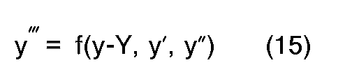
- the time T can be minimized with bang-bang control of y′′′. That is, y′′′ assumes its maximum value W, its minimum value -W, or a zero value. Algebraically: depending on y(t), y′(t) and y ⁇ (t). The theory also indicates that there are at most two switches between +W and -W in any given solution. See Lee and Markus, Foundations of Optimal Control Theory , John Wiley and Sons, Inc., 1968, incorporated herein by reference.
- the term y′′′(t) is zero whenever the velocity limit V or the acceleration limit A is controlling.
- a region D of permissible combinations of y′ and y ⁇ is defined.
- the region D thus represents a path limitation based on the physical constraints of the servo system.
- the main objective of path generation is to define the minimum time path, realizing that the physical constraint region of Figure 3 may operate to alter the optimum trajectory.
- the curve C is effectively split into two disjoint regions: a C+ region designated by the trace 42 and a C ⁇ region designated by the trace 44.
- the sign of the term y′′′ is switched when the respective region of the C curve is hit.
- the surface S and its relationship to the curve C is graphically depicted in Figure 5.
- /2W] 0 and ⁇ y ⁇ ⁇ 0.
- /2W] 0 and ⁇ y ⁇ ⁇ 0.
- the curve C and surface S have been defined assuming that, once the trajectory is on the surface S, the acceleration limit cannot be violated.
- FIG. 6 depicts the (y ⁇ , y′) projection of a representative trajectory 46 and a final approach C curve 48/50 which intersects parabolic upper and lower limits 34 and 32 of the D region.
- y′′′ +W
- the trajectory 46 increases in velocity and acceleration until the surface S ⁇ is hit at point 1.
- y′′′ -W is used and the trajectory 46 follows the surface S ⁇ until it hits the final approach C curve 48.
- the term y′′′ is switched to +W and the trajectory follows the projected C curve 48 to the target position.
- the projected C curve flattens and intersects the acceleration limits of the D region, as depicted by the broken trace 52/54.
- the acceleration limit A may be encountered before the trajectory hits the C curve, as depicted in Figure 6 by the broken trace 56.
- the term y′′′ must be set equal to zero to prevent a violation of the limit, and the trajectory follows the vertical acceleration limit before hitting and following the final approach C curve 52 to the target position.
- the limit situation described above is handled by (1) modifying the C curve to form a new curve designated as C and (2) modifying the S surface to form a new surface designated S .
- the modified projected curve C includes a parabolic segment, as in the normal curve C, and a vertical segment created by the acceleration limit A.
- the modified C ⁇ curve can be defined as the set of all points (y ⁇ , y′, y
- the difficulty lies in detecting the exact intersection of the trajectory with the surfaces, curves and constraints at which y′′′ must be changed. This is true with respect to the surface S , the curve C and the constraint surfaces of region D. Since a digital arrangement operates at a discrete time update rate, the exact moment of a surface crossing will not, in all probability, coincide with a sample time. For example, if the apparatus has a sample interval of dt seconds and y is above the surface S , the switch of y′′′ from +W to -W will likely occur late (up to dt seconds) and the trajectory of (y ⁇ , y′, y) will overshoot the surface S .
- the triple (y ⁇ , y′, y-Y) will lie either above or below the surface S following the switch. Potentially, this results in a limit cycle in the path position y as y′′′ alternates between -W and +W -- an unacceptable mode of operation.
- past values of S and y are used to predict future ones.
- S ⁇ (t+dt) ⁇ 5 2 S ⁇ (t) - 2 S ⁇ (t-dt) + 1 2 S ⁇ (t-2dt)
- y(t+dt) ⁇ 5 2 y(t) - 2y(t-dt) + 1 2 y(t-2dt).
- the term y′′′ must be switched from +W if y(t+dt) ⁇ S(t+dt) in order to avoid an overshoot of the surface S .
- y′′′(t) -W + DEL (37)
- DEL is defined such that the rate of change in error e s ′(t) between the surface S and the trajectory y is approximately proportional to e s (t), with a constant proportionality factor.
- the error e s (t) decays approximately exponentially, beginning at the sample interval dt for which an impending overshoot is detected.
- a similar control problem occurs with respect to the curve C once the trajectory is on the surface S .
- the objective is to avoid an overshoot of the curve C .
- the solution to the problem of hitting the curve C is similar to that of hitting the surface S , in that the value of y′′′ is modified to assume a value between +W and -W.
- the expressions for curve C are much easier to compute than the expressions for surface S , enabling the control unit 22 to employ a more exact solution.
- the position is y(t)
- the velocity is y′(t)
- the acceleration is y ⁇ (t).
- INT[x] is defined as the largest integer less than or equal to x.
- N INT[
- the path generation technique described above is periodically performed by the control unit 22 of Figure 1 to recursively generate a desired or commanded trajectory.
- the function is embodied in a computer program routine referred to herein as MINTIME, such routine being described herein in reference to the flow diagrams of Figures 7 - 23.
- ISTATE The status of the trajectory relative to the respective target surface, curve and position is indicated by a term ISTATE.
- ISTATE is advantageously used to avoid recurring calculations and unplanned switches in y′′′ between -W and +W.
- ISTATE is set to zero and initial conditions are defined.
- the initial trajectory components y(0)-Y, y′(0) and y ⁇ (0) are then used to determine which surface component S+ or S ⁇ is appropriate; see Figure 7.
- IBOUND is used to indicate whether unmodified or modified surfaces S, S and curves C, C are appropriate. IBOUND is set to 1 when the unmodified surface S and curve C may be used, and to 2 when the modified surface S and curve C must be used. and IBOUND is set to 2.
- the computed surface is compared to the initial trajectory position, y(0)-Y; see Figure 10. If the trajectory is below the surface, ISTATE is set to 1; if the trajectory is above the surface, ISTATE is set to 2; and if the trajectory is on the surface, ISTATE is set to 7.
- the control unit determines the proper value of y′′′. If an overshoot of the surface S is impending, the term ISTATE is set to 7, and the flow diagram of Figure 17 is executed to modify y′′′ so that the trajectory exponentially approaches the surface. If the trajectory has hit the velocity constraint V, ISTATE is set equal to 5 or 6. If the trajectory has hit the acceleration constraint A, ISTATE is set equal to 3 or 4. If an overshoot of either constraint is impending, the control unit interpolates to the constraint curve by determining an appropriate value for y′′′ between -W and +W. See Figures 11 or 12. Thereafter, the flow diagrams of Figures 21 or 22 are executed to update the trajectory components y, y′ and y ⁇ by integration.
- Figures 24 - 28 Representative trajectories generated by the MINTIME routine are graphically illustrated in Figures 24 - 28.
- Figure 24 illustrates the monotonicity of the trajectory beginning and ending at rest.
- the acceleration limit A was chosen so large that it would not apply.
- Figure 25 both acceleration and velocity limits apply.
- Figures 26 - 28 the initial position is not at rest.
- the detection of an impending crossover is indicated by a "rounding off" of the ideal square-wave behavior of y'''(t). Other deviations from ideal square-wave behavior of y''' are due to the cubic approximation of the final approach curve C.
- the path following function of this invention is set forth in terms of motor voltage control, as opposed to motor current control.
- Voltage control is preferred (at least in applications having variable load torque requirements) because, unlike current control, it is relatively insensitive to changes in the load torque. While it can be sensitive to changes in motor speed, an accurate measure of motor speed can be readily obtained.
- the third-order character of expressions (58) and (59) requires that the commanded trajectory also be third-order. In other words, the third derivative y′′′ of the commanded position y must be bounded. By definition, the trajectory developed by the path generation set forth herein satisfies this criteria.
- the reference or commanded trajectory is tracked using feedback terms based on the tracking error and its rate of change, feedforward terms based on the tracking error e(t), the trajectory components y′, y ⁇ and y′′′, and the static friction term V f .
- u(t) u e (t) + v3 y′′′(t) + v2 y ⁇ (t) + v1 y′(t) + (v f -V f ) (61)
- the feedforward parameters v1 - v3 relate to physical parameters of the motor, as defined above, and are tuned in real time according to this invention, to drive expression (61) into conformance with the physical system.
- the feedforward parameters are individually adjusted in proportion to the product of the tracking error and the respective multiplier of expression (61).
- the parameter v1 is adjusted in relation to the product of e(t) and y′(t).
- v f The static friction term v f is directionally dependent. It has a value of +v4 if y′ > 0, and -v5 if y′ ⁇ 0.
- the feedforward terms ensure substantially zero tracking error within the dynamic capability of the DC servomotor 12 by anticipating the dynamics of the trajectory.
- the dynamics of the trajectory are immediately reflected in the control voltage u(t) of the DC servomotor.
- the coefficients v1 - v5 are uniquely determined by the physical characteristics of the DC servomotor 12 and load, as well as the control unit and feedback sampling rate. Motor-to-motor and day-to-day variations in the characteristics, and hence the coefficients, are compensated for by the adaptive adjustment since the adjustment is based on the tracking error and the command derivatives. As a result, the motion control apparatus can track the third-order trajectory with virtually zero tracking error.
- FIG. 29 A diagram illustrating the path following function of this invention in control apparatus format is depicted in Figure 29.
- the path generation function provides the y′′′ limitation from which y ⁇ , y′ and y are computed by successive integration.
- the tracking error e(t) is determined according to the difference between the path position y and the feedback motor position x, and used to compute the various terms v1 - v5.
- the feedback, static friction and feedforward voltages are summed to form a control voltage V, which is applied to the DC voltage-mode power amplifier 16 for suitably energizing the DC servomotor 12.
- FIG. 30 A flow diagram for carrying out the motion control functions of this invention is set forth in Figure 30.
- the block 100 in Figure 30 generally designates a series of program instructions executed at the initiation of each period of servo operation for initializing the values of various terms and registers.
- the term ISTATE of the path generation routine is set to zero, and the feedforward parameters v1 - v5 are set to a predetermined estimate of their true value, or to values "learned" in a prior period of operation.
- a real time clock is started as indicated by the step 102, and the instruction steps 104 - 120 are repeatedly executed in sequence as indicated by the flow diagram lines 122.
- Steps 108 - 120 operate in connection with the real time clock and an interrupt counter (INT COUNTER) to set the execution rate of steps 104 - 116.
- INT COUNTER interrupt counter
- the minimum time path generation and adaptive feedforward tracking routines described herein were implemented together on a Motorola 68000 microprocessor with floating point firmware.
- the objectives of minimum time to target, substantially no following error and substantially no overshoot, were achieved with a main loop cycle time of approximately 5.25 milliseconds.
- FIGS 31 and 32 graphically depict the improvements observed in an application of the above mechanization to the waist axis servo mechanism of a conventional industrial robot.
- Each Figure depicts the operation of the servo mechanism at full rated speed with both a conventional motion control apparatus and the subject motion control apparatus.
- Figure 31 depicts the actual acceleration of the servo mechanism, using equal acceleration scales and a common time base.
- the conventional control (Graph a) is second-order and commands step changes in the acceleration, as indicated by the broken trace.
- the servo mechanism cannot achieve the step change and there is a large initial error, followed by an overshoot and damped oscillation.
- the same phenomena occur when the deceleration is commanded at time t2. In practice, this results in unsteadiness and overshoot of the target position.
- the control of this invention (Graph b) is third-order and results in a trackable acceleration command.
- the acceleration of the servo follows the commanded value, with substantially no overshoot of the target position.
- the motor voltage and current traces (not shown) have similar profiles.
- Figure 32 depicts the servo mechanism end of travel oscillation, as measured at the tip of a resilient servo load (end effector). Such oscillation corresponds to the settling time of the load once the target position has been achieved.
- the conventional control Graph a
- the oscillation is much smaller and damps out to substantially the same level after two seconds.
- the faster settling time achieved with the motion control apparatus of this invention permits increased cycle time in applications such as spot welding where significant load oscillation is not permitted.
- the reduced number and amplitude of the attendant torque reversals results in improved life of the servo mechanism.
Landscapes
- Engineering & Computer Science (AREA)
- Human Computer Interaction (AREA)
- Manufacturing & Machinery (AREA)
- Physics & Mathematics (AREA)
- General Physics & Mathematics (AREA)
- Automation & Control Theory (AREA)
- Feedback Control In General (AREA)
- Control Of Position Or Direction (AREA)
Description
- This invention relates to motion control apparatus for a servo mechanism and more particularly to a digital path generation and tracking method for quickly moving a positionable member to a commanded position with negligible following error and substantially no overshoot, independent of speed, within the servomotor capability.
- Broadly, this invention pertains to a servo mechanism system of the type which moves an output member, such as a robot arm, in accordance with a target position. Functionally, this involves detecting the actual position of the output member, defining a desired trajectory or path for achieving the target position, determining an actuator command, based on the position error and the desired trajectory, and activating the servo mechanism in accordance with the actuator command. When the servo mechanism is a DC servomotor, the actuator command is typically determined in terms of armature current or velocity and is carried out using closed-loop control techniques.
- A motion control apparatus in accordance with the present invention is characterised by the features specified in the characterising portion of
Claim 1. - More specifically, the present invention pertains to a method and apparatus for activating a servo mechanism for tracking a third-order trajectory with substantially no tracking error. Tracking or following errors are a direct result of conventional feedback control apparatus, where the actuator commands are determined as a function of the error between the commanded position (trajectory) and the actual position. This includes so-called proportional-plus-derivative controllers, where the actuator command is determined as a linear combination of the position error and measured motor velocity.
- Following errors tend to increase with increasing load and also with increasing commanded speed and acceleration. The error can be significant because command positions are coordinated (for example, straight-line) while following error is not. Following errors represent a deviation of the output member from the intended trajectory, and the deviation is usually maintained within "acceptable" limits by imposing additional limitations on the peak speed and acceleration of the trajectory. This results in further underutilization of the servo mechanism and further increases the time required to achieve the target position.
- This invention overcomes the problem of tracking or following errors with a novel adaptive feedforward control method which is capable of tracking well-defined third-order paths with substantially zero error. A motor voltage command Vm is determined in accordance with the sum of a feedback term based on the position error and a feedforward term based on the dynamics of the commanded position. The feedback term ensures the overall system stability, while the feedforward term ensures substantially zero following error within the dynamic capability of the servo mechanism by anticipating the dynamics of the commanded position.
- For a servomotor under simple inertial load, the feedforward term is in the form of a linear combination of the first three command derivatives --that is, the commanded velocity, acceleration and rate of change of acceleration. The coefficients of such derivatives are uniquely determined by the physical characteristics of the servomotor and load, as well as the controller and feedback sampling rate. Motor-to-motor and day-to-day variations in the characteristics, and hence the coefficients, are compensated for by adaptively adjusting the coefficients in real time, based on the tracking error and the command derivatives. As a result, the motion control apparatus can track the third-order trajectory with virtually zero error.
- The feedforward control of this invention is described herein in connection with a third-order path generation technique, the subject of our co-pending patent application no. (Our Ref: MJD/3036), filed the same day as the present application.
- Figure 1 is a schematic diagram of a motion control apparatus in accordance with this invention.
- Figures 2 - 6 are graphs referred to in the description of the theoretical path generation solution.
- Figures 7 - 23 are flow diagrams representative of computer program instructions executed by the control unit of Figure 1 in carrying out the path generation function.
- Figures 24 - 28 are graphs depicting the operation of the third order path generation function.
- Figure 29 is a control apparatus diagram of the adaptive feedforward control of this invention.
- Figure 30 is a flow diagram representative of computer program instructions executed by the control unit of Figure 1 in mechanizing the adaptive feedforward control of this invention.
- Figures 31 and 32 are graphic illustrations of the improvements observed when using the present invention.
- Referring now to the drawings, and more particularly to Figure 1, the
reference numeral 10 schematically designates a positionable member of a servo mechanism according to this invention. Thepositionable member 10 could take the form of an industrial robot arm, as in the illustrated embodiment, or any other position-controlled (output) member, such as a plotter arm, an engine throttle, etc. Aconventional DC servomotor 12 defines a servo mechanism which is rigidly coupled to thepositionable member 10 viashaft 14 and is adapted to be energized by a (DC voltage mode)power amplifier 16 for effecting movement of thepositionable member 10. TheDC servomotor 12 is also coupled to a position feedback sensor 18, such as a resolver or optical encoder, which provides an electrical signal indicative of the motor position online 20. - The reference numeral 22 generally designates a control unit, which is computer-based, according to this invention for controlling the output voltage of the
power amplifier 16 in response to the output of position feedback sensor 18 so as to move thepositionable member 10 from an initial position to a target position at rest in minimum time with substantially no overshoot or following errors. The control unit 22 represents an aggregate of conventional elements, including a central processing unit, a crystal controlled clock, read-only and random-access memory, digital and analogue input/output ports and D/A and A/D converter channels. The control unit 22 also supports auser interface 24, such as a video display terminal, to facilitate operator input of commanded positions and apparatus parameters. - The control unit 22 performs two primary functions in carrying out the objectives of this invention -- path generation and path following. Path generation refers to the derivation of a commanded trajectory in phase space between an initial position and a target position. Path following refers to the control of the motor voltage for effecting movement of the
positionable member 10 in accordance with the desired trajectory. Since the path generation routine is recursive, the control unit 22 periodically performs both functions while moving thepositionable member 10. In each execution period, the path generation routine updates the desired path, and the path following routine determines the required motor voltage for accurate following of the path. - It should be understood that the path following function of this invention will perform advantageously with a different and conventional path generation routine, so long as the rate of change of acceleration (jerk) remains substantially bounded. As indicated above, it is illustrated below in connection with a minimum time path generation function that is the subject of our above mentioned co-pending patent appliction. The path generation and path following functions are addressed separately below prior to a discussion of the illustrated embodiment wherein both functions are implemented by the single computer-based control unit 22.
- As with any good path, the third-order path y for the servo mechanism of this invention must be within the capabilities of the DC servomotor. The limits of the DC servomotor are defined by velocity, acceleration and jerk limits V, A and W, respectively. The velocity limit V arises from the motor voltage limit and the acceleration limit A arises from the motor current limit. The jerk limit W arises from the ability of the servo mechanism to tolerate mechanical compliance and the ability of the power source to supply the demanded rate of change of current. In addition to not violating motor and supply performance limitations, however, the illustrated path minimizes the transit time to a specified target position and hit the target position at rest. Given that T is the total transit time and t the instantaneous time, the problem can be stated algebraically as follows.
- Minimize T such that:


for 0 ≦ t ≦ T, and for prespecified bounds of V, A and W. - Applying conventional control theory, the time T can be minimized with bang-bang control of y‴. That is, y‴ assumes its maximum value W, its minimum value -W, or a zero value. Algebraically:

depending on y(t), y′(t) and y˝(t). The theory also indicates that there are at most two switches between +W and -W in any given solution. See Lee and Markus, Foundations of Optimal Control Theory, John Wiley and Sons, Inc., 1968, incorporated herein by reference. - A discussion of the theoretical solution, entitled, "A New Approach to Minimum Time Robot Control", was authored and published by the inventor hereof in the Proceedings of the Winter Annual Meeting of the ASME, November 17 - 22, 1985, Robotics and Manufacturing Automation, PED Vol. 15, also incorporated herein by reference.
- The bang-bang form of the minimum time solution means that the (y, y′, y˝) phase space can be divided into three regions: one in which


- Treating first the condition for which


and

Combining expressions (1) and (2) and representing the initial conditions as a constant K yields:

which defines a family of concave upward parabolas in the (y˝, y′) plane, as graphically depicted by the traces 30 - 32 in Figure 2. Since y‴ > 0, y˝ is increasing and the parabolas are traversed from left to right as indicated. - Since |y′| must be less than or equal to the motor velocity limit V, the lower constraint y′ ≧ -V in the (y˝, y′) plane is given by the expression:

This is the parabola 32 of Figure 2 which intersects the point
- A similar analysis for the condition of


which defines a family of concave downward parabolas in the (y˝, y′) plane, as graphically depicted by the traces 34 - 38 in Figure 2. Since y‴ < 0, y˝ is decreasing and the parabolas are traversed from right to left as indicated. - In this case (


This is theparabola 34 of Figure 2 which intersects the point
- When the
parabolas 32 and 34 are combined with the constraint that |y˝| be less than or equal to the motor acceleration limit A, a region D of permissible combinations of y′ and y˝ is defined. This region is graphically depicted in Figure 3, where the upper boundary is given by theparabola 34, the lower boundary is given by the parabola 32, the left-hand boundary is given by the acceleration limit of


- The acceleration-based limits are linear at

point 1 on the upper boundary is hit (as by the path 40), the maximum rate of deceleration (
point 2. A similar analysis applies to the lower boundary. - The main objective of path generation is to define the minimum time path, realizing that the physical constraint region of Figure 3 may operate to alter the optimum trajectory. To hit a target position Y at rest, the path y must traverse a parabola, in the (y˝, y′) plane, intersecting the point


and

Expressions (9) and (10) define a "final approach" curve C in the (y˝, y′, y) phase space containing the set of all points (y˝, y′, y) which can be steered to the target of

trace 42 and a C⁻ region designated by the trace 44. The C⁻ region represents a final approach curve for hitting the target position Y at rest with
 .
.
- The surface S⁺ is defined as the set of all points (y˝, y′, y) which can be steered to the curve C⁻ with
 , and a surface S⁻ as the set of all points (y˝, y′, y) which can be steered to the curve C+ with
 . In either case, the sign of the term y‴ is switched when the respective region of the C curve is hit. The surface S and its relationship to the curve C is graphically depicted in Figure 5.
- Mathematically, the surface S⁺ can be defined as the set of all points (y˝, y′, y) such that:

if


Similarly, the surface S⁻ can be defined as the set of all points (y˝, y′, y) such that:

if


Since the minimum time solution requires, at most, two switches of y‴ between +W and -W, it follows that for points above the surface S,
 would then be used on the S+ surface until the curve C⁻ is hit, whereafter


- The remainder of the theoretical solution is directed toward defining y‴ (that is, +W, -W, or 0) in terms of the expressions for the surface S, the curve C and the region D. Intuitively, and from expressions (11) - (14), the proximity of a point (y˝, y′, y) to the surface S for any given target position Y, depends on y˝, y′ and y-Y; that is, the acceleration, the velocity and the relative distance to the target. The objective, then, is to define y‴ in the form:
- In view of the above, and without regard to velocity and acceleration constraints V and A, we can define y‴ as follows:


and


The curve C and surface S have been defined assuming that, once the trajectory is on the surface S, the acceleration limit cannot be violated. This condition is graphically illustrated in Figure 6, which depicts the (y˝, y′) projection of arepresentative trajectory 46 and a finalapproach C curve 48/50 which intersects parabolic upper andlower limits 34 and 32 of the D region. Assuming an initial at rest position below the surface S, and
trajectory 46 increases in velocity and acceleration until the surface S⁻ is hit atpoint 1. Thereafter,
trajectory 46 follows the surface S⁻ until it hits the finalapproach C curve 48. When the intersection occurs, the term y‴ is switched to +W and the trajectory follows the projectedC curve 48 to the target position. - Due to the relationship between the projected
C curve 48 and the D region, no trajectory within the upper andlower limits 34 and 32 will violate the acceleration limit
- With a larger value of W (that is, WV > A²), the projected C curve flattens and intersects the acceleration limits of the D region, as depicted by the broken trace 52/54. In such case, the acceleration limit A may be encountered before the trajectory hits the C curve, as depicted in Figure 6 by the broken trace 56. When this happens, the term y‴ must be set equal to zero to prevent a violation of the limit, and the trajectory follows the vertical acceleration limit before hitting and following the final approach C curve 52 to the target position.
- The limit situation described above is handled by (1) modifying the C curve to form a new curve designated as C and (2) modifying the S surface to form a new surface designated S. The modified projected curve C includes a parabolic segment, as in the normal curve C, and a vertical segment created by the acceleration limit A. The modified surface S represents the set of all points (y˝, y′, y) which can be steered to the modified curve C with

- As indicated above, the acceleration limit will only be encountered enroute to the C⁺ curve if the product WV > A², where V is the maximum velocity attained with


-- see expression (7) -- where the constant is the maximum velocity attained with

From expressions (9) and (10), the intersection of the previously defined curve C⁺ with the acceleration limit of

and

The vertical segment of the modified projected curve C⁺, then, corresponds to the set of points (y˝, y′, y) which can be steered to the intersection point defined by the expressions (19) and (20), with
 . Integrating


Summarizing, the modified C⁺ curve can be defined as the set of all points (y˝, y′, y) such that:


and


A similar analysis will show that the modified C⁻ curve can be defined as the set of all points (y˝, y′, y) such that:


and


As indicated above, the modified surface S⁻ is the set of all points (y˝, y′, y) which can be steered to the modified curve C⁺ with

is satisfied, the acceleration limit A will not be encountered and the unmodified surface S⁻ is valid. However, if

is satisfied, the acceleration limit A will be encountered and the surface S⁻ has to be modified (S⁻) to represent the set of all points that can be steered to the vertical segment of curve C⁺ with
- Given the condition that


and

where tc is the time at which the trajectory hits the modified curve C⁺. Since

and

Combining expressions (22) - (26), and suppressing the initial condition subscript yields an expression for the modified surface S⁻ as follows:

where tc is given by:

A similar analysis in relation to the modified curve C⁻ reveals that the modified surface S⁺ is given by the expression:

where tc is given by the expression:

Unfortunately, the theoretical solution is not adapted for direct mechanization in a digital, or discrete sampled, arrangement. The difficulty lies in detecting the exact intersection of the trajectory with the surfaces, curves and constraints at which y‴ must be changed. This is true with respect to the surface S, the curve C and the constraint surfaces of region D. Since a digital arrangement operates at a discrete time update rate, the exact moment of a surface crossing will not, in all probability, coincide with a sample time. For example, if the apparatus has a sample interval of dt seconds and y is above the surface S, the switch of y‴ from +W to -W will likely occur late (up to dt seconds) and the trajectory of (y˝, y′, y) will overshoot the surface S. In other words, the triple (y˝, y′, y-Y) will lie either above or below the surface S following the switch. Potentially, this results in a limit cycle in the path position y as y‴ alternates between -W and +W -- an unacceptable mode of operation. - The operation described above is avoided through an approximation of the path expressions which achieves the objective of hitting the target Y at rest without violating the apparatus constraints. The number of calculations per time step is minimized to facilitate real time generation of the path.
- In a digital implementation, the terms y, y′, y˝, y‴ are updated every dt seconds. It is assumed that y‴ is constant over each dt second interval between samples. For a given value of y‴(t), the terms y˝(t+dt), y′(t+dt) and y(t+dt) can be found by integration as follows:


When (y˝, y′, y-Y) lies below S, the term y‴ is set equal to +W. If y‴ were switched to -W after the intersection with the surface S, an overshoot would occur. If y‴ were switched to -W prior to the intersection with the surface S, the triple (y˝, y′, y-Y) would remain below the surface S and parallel thereto. This apparent dilemma is overcome by a technique which predicts the occurrence of surface crossings and suitably adjusts the value of y‴. - At any sample time dt, we assume that we have already computed y(t), y′(t) and y˝(t), by expressions (31) - (33). Therefore, at a sample time dt, the terms y′(t) and y˝(t) are used to compute a trajectory intersection point S(t) on the target surface S. If y(t) < S(t), the trajectory is below the surface S, and y‴ should be +W unless no overshoot will occur in the next interval dt.
- The likelihood of an overshoot occurring could be determined by computing y(t+dt) and S(t+dt) with

- According to the illustrated embodiment, past values of S and y are used to predict future ones. Using second order approximations:


With either embodiment, the term y‴ must be switched from +W if

For points below the surface S, y‴(t) may thus be defined as:

The term DEL is defined such that the rate of change in error es′(t) between the surface S and the trajectory y is approximately proportional to es(t), with a constant proportionality factor. With this constraint, the error es(t) decays approximately exponentially, beginning at the sample interval dt for which an impending overshoot is detected. If ts is defined as a time between sample intervals -- that is, t ≦ ts ≦ t+dt -- the error characteristic may be expressed algebraically as follows:

and by integration,

where G is the constant rate. Projected over an integral number n of intervals dt, the error es(t+ndt) may be expressed as follows:

In other words, the error es(t) decays at an exponential rate (1 - G dt). - With the above objective in mind, an expression for DEL is derived by relating the rate of change of error es′(t) to the surface and trajectory terms. It follows from expression (35) that:

For
 , yields an expression for S′(t) as follows:

Rearranging and combining expressions (36) and (38) yields an expression for DEL as follows:

In practice, we have achieved good results with

- For


where x is defined as:

Summarizing, when y begins below S and an overshoot either is about to occur or has occurred, the term y‴ is switched from +W to (-W + DEL), the term DEL being given by expression (42) when

and by expression (43) when

- Similarly, if y has been above the surface S, then a surface crossing between times t and t+dt -- that is,


to

Expressions for the term DEL are derived in a manner analogous to that described above with respect to trajectories initially above the surface S. The expressions for the term DEL relative to trajectories initially below the surface S for the conditions


and


- A similar control problem occurs with respect to the curve C once the trajectory is on the surface S. As with the approach to the surface S, the objective is to avoid an overshoot of the curve C. The solution to the problem of hitting the curve C is similar to that of hitting the surface S, in that the value of y‴ is modified to assume a value between +W and -W. However, the expressions for curve C are much easier to compute than the expressions for surface S, enabling the control unit 22 to employ a more exact solution.
- First, it is assumed that the trajectory is on the surface S⁻ and approaching curve C⁺. It is further assumed that

- Defining a term Q(t) as:

it follows that
- The expression for Q(t+dt) is as follows:

Rearranging,

Assume that in a given interval, an evaluation of Q(t+dt) indicates that an overshoot of the curve C is imminent with

which is assumed to be positive. For

which is assumed to be negative. Thus, for some value of y‴ between -W and +W

That value of y‴ is identified, in the illustrated embodiment, by a secant approximation, regarding Q as a function of y‴. While other methods including Newton's approximation or direct quadratic solution are available, the secant approximation is preferred because it is inherently stable and economizes on real time calculations. - In the secant approximation, P(w) is defined as:


- The secant approximation to


Solving for w when z = 0 yields an approximation to the root P(w) = 0:
Substituting P(-W) and P(+W) into expression (49) yields the value w for y‴ between -W and W that interpolates to the curve C:

Improved accuracy can be obtained, either by repeating the secant approximation using (49) as a new endpoint or by using

as one endpoint of the interpolation. That is, if P(0) > 0, then P(0) and P(-W) are used to determine the secant; if P(0) < 0, then P(0) and P(+W) are used to determine the secant. A similar analysis yields analogous formulas for hitting C⁻ from S⁺ when
- The approach to any curve in phase space or in the (y′, y˝) phase plane can be handled in the same manner. For example, if the trajectory is on S⁻ with


If expression (51) is satisfied, y‴ must be switched from -W to a new value. In this case, interpolation is not necessary and y‴ is determined according to the expression:

In subsequent intervals, y‴ is set equal to zero until it is determined that the trajectory would overshoot the curve C⁺ with y‴ = 0. Then, the trajectory is interpolated to the C⁺ curve using the secant approximation described above. - Once the trajectory is on the C+ curve, the target


- In the illustrated embodiment, the final approach curve C is simulated with a cubic approximation which permits the trajectory to hit the target position


For K = 1, 2, ..., N, let:

and

While on final approach to the target


Enroute to the target


and

for K = 1, 2, ..., N.
Clearly,

so that y hits the target Y, at rest, at time (t+Ndt). - Since the velocity and acceleration bounds V and A are manifested as curves in the (y˝, y′) phase plane, an impending crossover may be detected in the same manner as for the final approach curve C, and the value of y‴ is determined by interpolation to avoid overshooting. The routine is depicted in its entirety in the flow diagrams of Figures 7 - 23.
- The path generation technique described above is periodically performed by the control unit 22 of Figure 1 to recursively generate a desired or commanded trajectory. The function is embodied in a computer program routine referred to herein as MINTIME, such routine being described herein in reference to the flow diagrams of Figures 7 - 23.
- The status of the trajectory relative to the respective target surface, curve and position is indicated by a term ISTATE. As indicated in the following description, the term ISTATE is advantageously used to avoid recurring calculations and unplanned switches in y‴ between -W and +W.
- Initially, the term ISTATE is set to zero and initial conditions are defined. The initial trajectory components y(0)-Y, y′(0) and y˝(0) are then used to determine which surface component S⁺ or S⁻ is appropriate; see Figure 7.
- Then, the appropriate surface S(0) or S(0) is computed; see Figures 8 and 9. The term IBOUND is used to indicate whether unmodified or modified surfaces S, S and curves C, C are appropriate. IBOUND is set to 1 when the unmodified surface S and curve C may be used, and to 2 when the modified surface S and curve C must be used. and IBOUND is set to 2.
- Then, the computed surface is compared to the initial trajectory position, y(0)-Y; see Figure 10. If the trajectory is below the surface, ISTATE is set to 1; if the trajectory is above the surface, ISTATE is set to 2; and if the trajectory is on the surface, ISTATE is set to 7.
- Then, the control unit determines the proper value of y‴. If an overshoot of the surface S is impending, the term ISTATE is set to 7, and the flow diagram of Figure 17 is executed to modify y‴ so that the trajectory exponentially approaches the surface. If the trajectory has hit the velocity constraint V, ISTATE is set equal to 5 or 6. If the trajectory has hit the acceleration constraint A, ISTATE is set equal to 3 or 4. If an overshoot of either constraint is impending, the control unit interpolates to the constraint curve by determining an appropriate value for y‴ between -W and +W. See Figures 11 or 12. Thereafter, the flow diagrams of Figures 21 or 22 are executed to update the trajectory components y, y′ and y˝ by integration.
- On the next call of the subroutine MINTIME, the current value of ISTATE is used to route the logic flow in the appropriate sequence. For example, if ISTATE = 3/4, the flow diagram of Figure 13/14 is executed to check a possible surface overshoot. If detected, ISTATE is set to 7 and y‴ is modified as above so that the trajectory exponentially approaches the surface S. If the velocity constraint V is hit, the control unit interpolates to the constraint and sets ISTATE to 5. If the velocity constraint V has not been hit, ISTATE remains equal to 3 and y‴ is set equal to 0. Thereafter, the flow diagrams of Figures 21 or 22 are executed to update the trajectory components y, y′ and y˝ by integration, as above.
- If ISTATE = 5/6, the flow diagram of Figure 15/16 is executed to check an impending surface overshoot. If detected, ISTATE is set equal to 7, as above, and y‴ is modified so the trajectory exponentially approaches the surface S. If not, and y˝ = 0, then the trajectory is at peak velocity. In such case, y‴(t) is set to zero and y(t+ dt) is set equal to y(t) + y′(t) dt. If


- If ISTATE is set to 7, the flow diagrams of Figure 17 - 19 are executed to determine if there is an impending overshoot of the curve C. If not, the linear correction to y‴ based on y(t) - Y - S(t) is continued in accordance with expressions (37) and (43) or (44). If there is an impending overshoot of the curve C with IBOUND = 2, the trajectory is interpolated to the curve and the control unit sets ISTATE to 8 and y‴ = 0 until IBOUND returns to 1. Once on the curve C, ISTATE is set to 9 and the control unit computes the final approach cubic according to expressions (55) - (57). When the trajectory position y hits the target position Y at rest, ISTATE is set to 10.
- The ISTATE variable can be valuable for control purposes as well, since it indicates the progress of the path. For example, the moment ISTATE = 7 is reached, the path begins to decelerate to hit Y. This point could be interpreted as a signal for a change of target, in case a moving target is the real objective. Another case is ISTATE = 8, which indicates that the trajectory is on the final approach to the target position. In this case, the control unit could initiate a parallel operation which is to be coordinated with the attainment of
 at rest.
- Representative trajectories generated by the MINTIME routine are graphically illustrated in Figures 24 - 28. Figure 24 illustrates the monotonicity of the trajectory beginning and ending at rest. The acceleration limit A was chosen so large that it would not apply. In Figure 25, both acceleration and velocity limits apply. In Figures 26 - 28, the initial position is not at rest. In Figure 28, the initial velocity and acceleration are so large relative to the initial position that the path must overshoot the target (Y=0) and then return. This is the only way overshoot can occur. In each case, the detection of an impending crossover is indicated by a "rounding off" of the ideal square-wave behavior of y'''(t). Other deviations from ideal square-wave behavior of y''' are due to the cubic approximation of the final approach curve C.
- For a number of reasons, the path following function of this invention is set forth in terms of motor voltage control, as opposed to motor current control. Voltage control is preferred (at least in applications having variable load torque requirements) because, unlike current control, it is relatively insensitive to changes in the load torque. While it can be sensitive to changes in motor speed, an accurate measure of motor speed can be readily obtained.
- With the load torque insensitivity of voltage mode control, we have found that the motor dynamics -- not the load torque -- dominate the motion control apparatus behavior. For an armature controlled DC servomotor under inertial load such as the
DC servomotor 12 of Figure l, such dynamics can be algebraically expressed as follows:
where: - u =
- motor voltage
- R =
- armature resistance
- L =
- armature inductance
- J =
- motor plus load inertia
- KT =
- motor torque constant KT
- B =
- viscous damping constant
- Ke =
- back-EMF constant
- Tf =
- torque due to static friction
- x, x′, x˝ and x‴ =
- motor position, velocity, acceleration and jerk.
- For convenience, expression (58) is abbreviated to:


- The third-order character of expressions (58) and (59) requires that the commanded trajectory also be third-order. In other words, the third derivative y‴ of the commanded position y must be bounded. By definition, the trajectory developed by the path generation set forth herein satisfies this criteria.
- Assuming a reference or command path y(t) as defined above, the tracking error e(t) is defined as:

According to the path following function of this invention, the reference or commanded trajectory is tracked using feedback terms based on the tracking error and its rate of change, feedforward terms based on the tracking error e(t), the trajectory components y′, y˝ and y‴, and the static friction term Vf. Algebraically, this is expressed as follows:

The feedback term ue(t) is based on the tracking error e(t) defined in expression 60 and may be determined in any manner which renders stable the error equation:

This is the equation that results under the control of expression (61) with the assumption that

with g₁ and g₂ chosen for stability of expression (62). In such case, e˝(t), e′(t) and e(t) all converge asymptotically to zero and the motor position x will track the reference trajectory in terms of position y, velocity y′ and acceleration y˝. - The feedforward parameters v₁ - v₃ relate to physical parameters of the motor, as defined above, and are tuned in real time according to this invention, to drive expression (61) into conformance with the physical system. As explained below, the feedforward parameters are individually adjusted in proportion to the product of the tracking error and the respective multiplier of expression (61). For example, the parameter v₁ is adjusted in relation to the product of e(t) and y′(t). Algebraically:


where the subscript "0" designates the present value of the term and the subscript "+1" designates the value of the term for the next time step (i.e., dt seconds later). - The static friction term vf is directionally dependent. It has a value of +v₄ if y′ > 0, and -v₅ if y′ < 0. The terms v₄ and v₅ are adjusted as follows:
If (y′)₀ > 0, then


If (y′)₀ < 0, then


If (y′)₀ = 0, then v₄ and v₅ are unchanged. - In the manner described above, the feedforward terms ensure substantially zero tracking error within the dynamic capability of the
DC servomotor 12 by anticipating the dynamics of the trajectory. As a result, the dynamics of the trajectory are immediately reflected in the control voltage u(t) of the DC servomotor. The coefficients v₁ - v₅ are uniquely determined by the physical characteristics of theDC servomotor 12 and load, as well as the control unit and feedback sampling rate. Motor-to-motor and day-to-day variations in the characteristics, and hence the coefficients, are compensated for by the adaptive adjustment since the adjustment is based on the tracking error and the command derivatives. As a result, the motion control apparatus can track the third-order trajectory with virtually zero tracking error. - A diagram illustrating the path following function of this invention in control apparatus format is depicted in Figure 29. In that diagram, the path generation function provides the y‴ limitation from which y˝, y′ and y are computed by successive integration. The tracking error e(t) is determined according to the difference between the path position y and the feedback motor position x, and used to compute the various terms v₁ - v₅. The feedback, static friction and feedforward voltages are summed to form a control voltage V, which is applied to the DC voltage-
mode power amplifier 16 for suitably energizing theDC servomotor 12. - A flow diagram for carrying out the motion control functions of this invention is set forth in Figure 30. The
block 100 in Figure 30 generally designates a series of program instructions executed at the initiation of each period of servo operation for initializing the values of various terms and registers. For example, the term ISTATE of the path generation routine is set to zero, and the feedforward parameters v₁ - v₅ are set to a predetermined estimate of their true value, or to values "learned" in a prior period of operation. - Following initialization of the various terms and registers of control unit 22, a real time clock is started as indicated by the
step 102, and the instruction steps 104 - 120 are repeatedly executed in sequence as indicated by the flow diagram lines 122. Steps 108 - 120 operate in connection with the real time clock and an interrupt counter (INT COUNTER) to set the execution rate of steps 104 - 116. - The minimum time path generation and adaptive feedforward tracking routines described herein were implemented together on a Motorola 68000 microprocessor with floating point firmware. The objectives of minimum time to target, substantially no following error and substantially no overshoot, were achieved with a main loop cycle time of approximately 5.25 milliseconds.
- Figures 31 and 32 graphically depict the improvements observed in an application of the above mechanization to the waist axis servo mechanism of a conventional industrial robot. Each Figure depicts the operation of the servo mechanism at full rated speed with both a conventional motion control apparatus and the subject motion control apparatus.
- Figure 31 depicts the actual acceleration of the servo mechanism, using equal acceleration scales and a common time base. The conventional control (Graph a) is second-order and commands step changes in the acceleration, as indicated by the broken trace. When the acceleration is commanded at time t₁, the servo mechanism cannot achieve the step change and there is a large initial error, followed by an overshoot and damped oscillation. The same phenomena occur when the deceleration is commanded at time t₂. In practice, this results in unsteadiness and overshoot of the target position. The control of this invention (Graph b) is third-order and results in a trackable acceleration command. The acceleration of the servo follows the commanded value, with substantially no overshoot of the target position. The motor voltage and current traces (not shown) have similar profiles.
- Figure 32 depicts the servo mechanism end of travel oscillation, as measured at the tip of a resilient servo load (end effector). Such oscillation corresponds to the settling time of the load once the target position has been achieved. With the conventional control (Graph a), there is pronounced oscillation which damps out to a relatively low level after approximately six seconds. With the control of this invention (Graph b), the oscillation is much smaller and damps out to substantially the same level after two seconds. The faster settling time achieved with the motion control apparatus of this invention permits increased cycle time in applications such as spot welding where significant load oscillation is not permitted. Moreover, the reduced number and amplitude of the attendant torque reversals results in improved life of the servo mechanism.
- While this invention has been described herein in reference to the illustrated embodiment, it will be understood that various modifications will occur to those skilled in the art. For example, the path tracking function of this invention is equally applicable to hydraulic servo apparatus or electrical servo apparatus incorporating an AC servo motor.
Claims (2)
- A motion control apparatus including a servo mechanism (12) adapted to adjust the position of an output member (10) in relation to a control voltage applied thereto, path generation means (22) for defining third order trajectory position, velocity and acceleration parameters y, y′, and y˝ for steering the output member from its current position to a target position, and path tracking means (22) for supplying a control voltage to the servo mechanism for causing the output member to track the trajectory, characterised in that the path tracking means (22) includes feedback means (18,22) for computing the tracking error e according to the deviation of the output member (10) from the trajectory position parameter y, and for generating a feedback term in relation thereto;
feedforward means (22) for generating a feedforward term to be combined with the feedback term to form the servo mechanism control voltage, the feedforward term being determined substantially in accordance with the expression:

where the coefficients v₁, v₂, v₃ and vf relate to characteristic operating parameters of the motion control apparatus, whereby the dynamics of the trajectory are immediately reflected in the servo mechanism control voltage; and
adaptive means (22) for adjusting the value of the feedforward coefficients v₁, v₂, v₃ and vf substantially according to the expressions:


where k₁, k₂, k₃ and kf are constants, thereby to adaptively tune the feedforward coefficients v₁, v₂, v₃ and vf for a specific motion control apparatus, and to compensate for variations in the characteristic operating parameters thereof, allowing the trajectory to be tracked with minimum tracking error. - A motion control apparatus as claimed in Claim 1, wherein the servo mechanism (12) is operable in both forward and reverse directions;
the coefficient vf generated by the feedforward means (22) represents the static friction of the servo mechanism and comprises first and second additive terms v₄ and v₅ pertaining to forward and reverse operation of the servomotor, respectively; and
the adaptive means (22) includes means effective (1) when the sign of the trajectory velocity parameter y′ corresponds to forward movement of the servomotor to adjust the term v₄ substantially according to the expression:

where k₄ is a constant, and (2) when the sign of the trajectory velocity parameter y′ corresponds to reverse movement of the servo mechanism to adjust the term v₅ substantially according to the expression:

where k₅ is a constant.
Applications Claiming Priority (2)
| Application Number | Priority Date | Filing Date | Title |
|---|---|---|---|
| US45129 | 1987-05-01 | ||
| US07/045,129 US4761595A (en) | 1987-05-01 | 1987-05-01 | Motion control system having adaptive feedforward path tracking |
Publications (3)
| Publication Number | Publication Date |
|---|---|
| EP0289151A2 EP0289151A2 (en) | 1988-11-02 |
| EP0289151A3 EP0289151A3 (en) | 1990-06-06 |
| EP0289151B1 true EP0289151B1 (en) | 1994-01-12 |
Family
ID=21936143
Family Applications (1)
| Application Number | Title | Priority Date | Filing Date |
|---|---|---|---|
| EP88303068A Expired - Lifetime EP0289151B1 (en) | 1987-05-01 | 1988-04-06 | Motion control apparatus having adaptive feedforward path tracking |
Country Status (4)
| Country | Link |
|---|---|
| US (1) | US4761595A (en) |
| EP (1) | EP0289151B1 (en) |
| JP (1) | JPS63285601A (en) |
| DE (1) | DE3886989T2 (en) |
Cited By (1)
| Publication number | Priority date | Publication date | Assignee | Title |
|---|---|---|---|---|
| DE19922314A1 (en) * | 1999-05-14 | 2000-11-16 | Abb Patent Gmbh | Positioning drive regulating method involves five point element generating open or close command outside dead zone in addition to torque signal; output signals are used to control drive |
Families Citing this family (35)
| Publication number | Priority date | Publication date | Assignee | Title |
|---|---|---|---|---|
| JPS643705A (en) * | 1987-06-26 | 1989-01-09 | Toshiba Corp | Process controller |
| US4916635A (en) * | 1988-09-12 | 1990-04-10 | Massachusetts Institute Of Technology | Shaping command inputs to minimize unwanted dynamics |
| US4974210A (en) * | 1989-05-01 | 1990-11-27 | General Electric Company | Multiple arm robot with force control and inter-arm position accommodation |
| JPH0324606A (en) * | 1989-06-22 | 1991-02-01 | Yutaka Kanayama | Method for specifying route of moving robot |
| JP3002206B2 (en) * | 1989-06-22 | 2000-01-24 | 神鋼電機株式会社 | Travel control method for mobile robot |
| JPH03118618A (en) * | 1989-09-30 | 1991-05-21 | Fanuc Ltd | Control system applying sliding mode control having damping effect |
| JP2657561B2 (en) * | 1990-02-09 | 1997-09-24 | 富士通株式会社 | Positioning control method |
| DE4040796A1 (en) * | 1990-12-17 | 1992-07-02 | Mannesmann Ag | METHOD FOR ADAPTIVE CONTROL OF POSITIONABLE DRIVES |
| JP2840139B2 (en) * | 1991-04-24 | 1998-12-24 | ファナック株式会社 | Foreseeable repetition control device |
| US5249118A (en) * | 1991-09-03 | 1993-09-28 | Golden Gate Microsystems Incorporated | Fully adaptive velocity tracking drive control positioning system |
| JPH0561506A (en) * | 1991-09-04 | 1993-03-12 | Satoshi Tsuboi | Foreknowledge control method for action controller |
| EP0596141A4 (en) * | 1992-05-22 | 1994-11-30 | Fanuc Ltd | Control method for servomotor. |
| US5508596A (en) * | 1993-10-07 | 1996-04-16 | Omax Corporation | Motion control with precomputation |
| JP3593850B2 (en) * | 1996-06-17 | 2004-11-24 | トヨタ自動車株式会社 | Tool point sequence generation method |
| WO1998015880A1 (en) * | 1996-10-08 | 1998-04-16 | Siemens Aktiengesellschaft | Method and control structure for controlling moments in numerically controlled elastic (and therefore oscillation-capable) multiple mass systems |
| DE19811346A1 (en) * | 1998-03-16 | 1999-09-30 | Siemens Ag | Signal processing method |
| JP3481468B2 (en) * | 1998-09-30 | 2003-12-22 | 三菱電機株式会社 | Electric power steering device |
| DE19913870A1 (en) * | 1999-03-26 | 2000-10-19 | Siemens Ag | Positioning sensor used for operating electromagnetic control of valves has a capacitor coupled to a lifting movement |
| DE19913869A1 (en) * | 1999-03-26 | 2000-10-19 | Siemens Ag | Position sensor for controlling electromagnetically-operated valves; lifts object to be moved with instant lift by judging change in inductance arising from lifting movement |
| US6661599B1 (en) | 1999-08-27 | 2003-12-09 | Seagate Technology Llc | Enhanced adaptive feedforward control to cancel once-per-revolution disturbance by shaping the internal mode |
| FR2835067B1 (en) * | 2002-01-21 | 2004-04-02 | Trw Sys Aeronautiques Civil | CONTROL DEVICE WITH LOOP, IN PARTICULAR ELECTRO-HYDRAULIC FLIGHT CONTROL ACTUATOR |
| JP3875988B2 (en) * | 2002-05-10 | 2007-01-31 | 本田技研工業株式会社 | Real-time tracking of unpredictable targets in unknown obstacles |
| DE10359412B4 (en) * | 2003-12-18 | 2015-11-26 | Robert Bosch Gmbh | A method of calculating a transition curve for transitioning a controlled variable from an initial value to a final value |
| US20070142966A1 (en) * | 2005-12-20 | 2007-06-21 | Khalid Mirza | Process for moving a robot |
| US7609813B2 (en) * | 2006-11-08 | 2009-10-27 | General Electric Company | System and method for improved collision detection in an imaging device |
| US7479751B2 (en) * | 2007-01-29 | 2009-01-20 | Rockwell Automation Technologies, Inc. | Elimination of unintended velocity reversals in s-curve velocity profiles |
| DE102007061323A1 (en) * | 2007-12-19 | 2009-07-02 | Kuka Roboter Gmbh | Method for controlling the movement of a robot within a workspace |
| US20090237749A1 (en) * | 2008-03-24 | 2009-09-24 | Abb Ltd. | Dynamic Set-Point Servo Control |
| CN101850549B (en) * | 2010-04-30 | 2011-12-28 | 苏州博实机器人技术有限公司 | Special joint feature detection and parameter regulation device for robot |
| US9381643B2 (en) | 2014-07-03 | 2016-07-05 | GM Global Technology Operations LLC | Dynamical system-based robot velocity control |
| US9592608B1 (en) * | 2014-12-15 | 2017-03-14 | X Development Llc | Methods and systems for providing feedback during teach mode |
| US9919422B1 (en) | 2016-01-06 | 2018-03-20 | X Development Llc | Methods and systems to provide mechanical feedback during movement of a robotic system |
| US10859997B1 (en) | 2017-12-04 | 2020-12-08 | Omax Corporation | Numerically controlled machining |
| US11554461B1 (en) | 2018-02-13 | 2023-01-17 | Omax Corporation | Articulating apparatus of a waterjet system and related technology |
| US11392104B2 (en) * | 2020-07-23 | 2022-07-19 | Mitsubishi Electric Research Laboratories, Inc. | System and method for feasibly positioning servomotors with unmodeled dynamics |
Family Cites Families (2)
| Publication number | Priority date | Publication date | Assignee | Title |
|---|---|---|---|---|
| US3838325A (en) * | 1973-08-30 | 1974-09-24 | K Kobayashi | Motor speed acceleration-deceleration control circuit |
| US4663726A (en) * | 1985-04-15 | 1987-05-05 | General Electric Co. | Robot control utilizing cubic spline interpolation |
-
1987
- 1987-05-01 US US07/045,129 patent/US4761595A/en not_active Expired - Lifetime
-
1988
- 1988-04-06 EP EP88303068A patent/EP0289151B1/en not_active Expired - Lifetime
- 1988-04-06 DE DE88303068T patent/DE3886989T2/en not_active Expired - Fee Related
- 1988-05-02 JP JP63109867A patent/JPS63285601A/en active Pending
Cited By (1)
| Publication number | Priority date | Publication date | Assignee | Title |
|---|---|---|---|---|
| DE19922314A1 (en) * | 1999-05-14 | 2000-11-16 | Abb Patent Gmbh | Positioning drive regulating method involves five point element generating open or close command outside dead zone in addition to torque signal; output signals are used to control drive |
Also Published As
| Publication number | Publication date |
|---|---|
| DE3886989T2 (en) | 1994-04-28 |
| EP0289151A2 (en) | 1988-11-02 |
| JPS63285601A (en) | 1988-11-22 |
| US4761595A (en) | 1988-08-02 |
| DE3886989D1 (en) | 1994-02-24 |
| EP0289151A3 (en) | 1990-06-06 |
Similar Documents
| Publication | Publication Date | Title |
|---|---|---|
| EP0289151B1 (en) | Motion control apparatus having adaptive feedforward path tracking | |
| EP0289150B1 (en) | Motion control method with minimum time path generation | |
| US5331264A (en) | Method and device for generating an input command for a motion control system | |
| EP0417312B1 (en) | Feedforward control unit for servomotor | |
| GB2119965A (en) | Manipulator with adaptive velocity controlled path motion | |
| Xu et al. | Implementation of VSS control to robotic manipulators-smoothing modification | |
| EP0790543B1 (en) | Method for switching a control mode of a servo control system | |
| US5373221A (en) | Method and system for estimating robot tool center point speed | |
| US6949905B2 (en) | Servo control system and method of setting | |
| KR0135308B1 (en) | Method of controlling servomotors | |
| WO2002025390A1 (en) | Servo control method | |
| KR970002259B1 (en) | Method for controlling servomotor | |
| Zeng et al. | An adaptive control strategy for robotic cutting | |
| JP3176003B2 (en) | Control device | |
| JPH07120215B2 (en) | Robot control method | |
| JP3541857B2 (en) | Overshootless auto tuning method | |
| Goor | A new approach to robot control | |
| JP3146550B2 (en) | Industrial robot control device | |
| JPH10149210A (en) | Method for preparing command for positioning control system | |
| Dahl | Path constrained robot control with limited torques-experimental evaluation | |
| Lee et al. | Efficient sliding mode control for robot manipulator with prescribed tracking performance | |
| Tang et al. | Knowledge-based extension of model-referenced adaptive control with application to an industrial process | |
| JPH01217601A (en) | Servo controller | |
| JP3427944B2 (en) | Trajectory tracking positioning control method | |
| KR920006163B1 (en) | Displacement control method |
Legal Events
| Date | Code | Title | Description |
|---|---|---|---|
| PUAI | Public reference made under article 153(3) epc to a published international application that has entered the european phase |
Free format text: ORIGINAL CODE: 0009012 |
|
| AK | Designated contracting states |
Kind code of ref document: A2 Designated state(s): DE IT SE |
|
| PUAL | Search report despatched |
Free format text: ORIGINAL CODE: 0009013 |
|
| AK | Designated contracting states |
Kind code of ref document: A3 Designated state(s): DE IT SE |
|
| RHK1 | Main classification (correction) |
Ipc: G05B 19/407 |
|
| 17P | Request for examination filed |
Effective date: 19900831 |
|
| ITTA | It: last paid annual fee | ||
| 17Q | First examination report despatched |
Effective date: 19930426 |
|
| GRAA | (expected) grant |
Free format text: ORIGINAL CODE: 0009210 |
|
| ITF | It: translation for a ep patent filed |
Owner name: BARZANO' E ZANARDO ROMA S.P.A. |
|
| AK | Designated contracting states |
Kind code of ref document: B1 Designated state(s): DE IT SE |
|
| REF | Corresponds to: |
Ref document number: 3886989 Country of ref document: DE Date of ref document: 19940224 |
|
| PLBE | No opposition filed within time limit |
Free format text: ORIGINAL CODE: 0009261 |
|
| STAA | Information on the status of an ep patent application or granted ep patent |
Free format text: STATUS: NO OPPOSITION FILED WITHIN TIME LIMIT |
|
| 26N | No opposition filed | ||
| EAL | Se: european patent in force in sweden |
Ref document number: 88303068.6 |
|
| PGFP | Annual fee paid to national office [announced via postgrant information from national office to epo] |
Ref country code: SE Payment date: 19950425 Year of fee payment: 8 |
|
| PGFP | Annual fee paid to national office [announced via postgrant information from national office to epo] |
Ref country code: DE Payment date: 19950526 Year of fee payment: 8 |
|
| PG25 | Lapsed in a contracting state [announced via postgrant information from national office to epo] |
Ref country code: SE Effective date: 19960407 |
|
| PG25 | Lapsed in a contracting state [announced via postgrant information from national office to epo] |
Ref country code: DE Effective date: 19970101 |
|
| EUG | Se: european patent has lapsed |
Ref document number: 88303068.6 |
|
| PG25 | Lapsed in a contracting state [announced via postgrant information from national office to epo] |
Ref country code: IT Free format text: LAPSE BECAUSE OF NON-PAYMENT OF DUE FEES;WARNING: LAPSES OF ITALIAN PATENTS WITH EFFECTIVE DATE BEFORE 2007 MAY HAVE OCCURRED AT ANY TIME BEFORE 2007. THE CORRECT EFFECTIVE DATE MAY BE DIFFERENT FROM THE ONE RECORDED. Effective date: 20050406 |