EP0125164A1 - Method of determining the characteristics of an underground formation producing fluids - Google Patents
Method of determining the characteristics of an underground formation producing fluids Download PDFInfo
- Publication number
- EP0125164A1 EP0125164A1 EP84400781A EP84400781A EP0125164A1 EP 0125164 A1 EP0125164 A1 EP 0125164A1 EP 84400781 A EP84400781 A EP 84400781A EP 84400781 A EP84400781 A EP 84400781A EP 0125164 A1 EP0125164 A1 EP 0125164A1
- Authority
- EP
- European Patent Office
- Prior art keywords
- theoretical
- experimental
- well
- graph
- fluid
- Prior art date
- Legal status (The legal status is an assumption and is not a legal conclusion. Google has not performed a legal analysis and makes no representation as to the accuracy of the status listed.)
- Granted
Links
Images


Classifications
-
- E—FIXED CONSTRUCTIONS
- E21—EARTH DRILLING; MINING
- E21B—EARTH DRILLING, e.g. DEEP DRILLING; OBTAINING OIL, GAS, WATER, SOLUBLE OR MELTABLE MATERIALS OR A SLURRY OF MINERALS FROM WELLS
- E21B49/00—Testing the nature of borehole walls; Formation testing; Methods or apparatus for obtaining samples of soil or well fluids, specially adapted to earth drilling or wells
- E21B49/008—Testing the nature of borehole walls; Formation testing; Methods or apparatus for obtaining samples of soil or well fluids, specially adapted to earth drilling or wells by injection test; by analysing pressure variations in an injection or production test, e.g. for estimating the skin factor
Definitions
- the present invention relates to hydrocarbon well tests, making it possible to determine the physical characteristics of the system formed by a well and an underground formation (also called “reservoir") producing hydrocarbons through the well. More specifically, the invention relates to a method according to which the flow of fluid produced by the well is modified by closing or opening a valve which is located on the surface or in the well. The resulting pressure variations are measured and recorded at the bottom of the well as a function of the time elapsed since the start of the tests, that is to say since the modification of the flow rate. The characteristics of the underground well-formation system can be deduced from these experimental data.
- the experimental data from the well tests are analyzed by comparing the response of the underground formation to a change in the flow rate of the fluid produced, with the behavior of theoretical models having well-defined characteristics and subjected to the same change in flow rate as the formation studied.
- the variations of pressure as a function of time characterize the behavior of the well-formation system and the removal at constant flow rate of fluids, by the opening of a valve in the initially closed well, is the test condition which is applied to training and theoretical model.
- the system studied and the theoretical model are identical both quantitatively and qualitatively. In other words, these tanks are assumed to have the same physical characteristics.
- the characteristics obtained from this comparison depend on the theoretical model: the more complicated the model, the more numerous the characteristics that can be determined.
- the basic model is represented by a homogeneous formation with upper and lower limits impermeable and with infinite radial extension. The flow in the formation is then radial, directed towards the well.
- the wall effect is defined by a coefficient S which characterizes the damage or stimulation of the part of the formation adjacent to the well.
- the compression or decompression effect of the fluid in the well is characterized by a coefficient C which results from the difference in fluid flow produced by the well, between the underground formation and the wellhead, when a valve located at the head well is either closed or open.
- the coefficient C is usually expressed in barrels per psi, one barrel being equal to 0.16m 3 and one psi equal to 0.069 bar.
- each curve is characterized by one or more dimensionless numbers which each represent a characteristic (or a combination of characteristics) of the theoretical system formed by a well and a reservoir.
- a dimensionless parameter is defined by the actual parameter (pressure for example) multiplied by an expression that includes certain characteristics of the well-reservoir system so as to make the dimensionless parameter independent of these characteristics.
- the coefficient S characterizes only the wall effect but is independent of the other characteristics of the reservoir and experimental conditions such as the flow rate, the viscosity of the fluid, the permeability of the formation, etc.
- the experimental curve and one of the standard curves represented with the same coordinate scales have an identical shape but are offset with respect to each other.
- the offsets along the two axes, on the ordinate for pressure and on the abscissa for time, are proportional to the characteristic values of the well-reservoir system which can thus be determined.
- Qualitative information on the underground formation is obtained by the identification of the different regimes on the graph in logarithmic scale representing the experimental data. Knowing that a particular characteristic of the well-reservoir system, such as for example a vertical fracture, is characterized by a particular regime, all the different regimes appearing on the graph of the experimental data are identified in order to select the appropriate model of well-reservoir system. . Specialized graphs taking into account only part of the experimental data allow the more precise determination of the characteristics of the system. We then return to the graph on a logarithmic scale taking into account all the data to confirm the choice of the system and the quantitative determination of the characteristics of the training. The latter are obtained by selecting a standard curve having the same shape as the experimental curve and by determining the offset of the coordinate axes of the experimental curve with respect to the theoretical curve.
- the patent of the United States of America 4,328,705 also describes a method according to which the standard curves are represented using the dimensionless pressure P for the ordinate axis and the ratio t D / C D for the abscissa axis, t D being dimensionless time and C D dimensionless coefficient characterizing the effect of compression or decompression of the fluid in the well.
- the disadvantage of the method described in this patent is that the standard curves have shapes varying relatively slowly with respect to each other. This results in a certain uncertainty in the choice of the standard curve corresponding to the experimental curve.
- the present invention relates to a method for determining the characteristics of a well-reservoir system allowing better identification between the experimental behavior of the analyzed system formed by the well and the underground formation and the behavior of a theoretical model.
- This model is general, namely that the formation can be homogeneous or heterogeneous and that it takes into account the wall effect and the effect of compression or decompression of the fluid and possibly the double porosity of the reservoir and fractures of the well.
- the method according to the present invention allows a global and unique analysis of the behavior of the well-reservoir system, without resorting to specialized analyzes.
- the invention also allows the analysis of experimental data when the condition imposed on the system is the closing of the well, thanks to a judicious choice of parameters.
- the method according to the present invention can also be advantageously combined with a method of the prior art.
- Said theoretical evolution can advantageously be that of the logarithm of the product P ' D ⁇ t D / C D as a function of the logarithm of t D / C D and said experimental evolution is that of the logarithm of the product ⁇ P'. ⁇ t as a function of the logarithm of ⁇ t.
- Said theoretical evolution can also be a function of an index representing a quantity characteristic of the product C D e 2S .
- said theoretical evolution can also be a function of an index representing a quantity characteristic of the product C D e 2S .
- the experimental curve correspond with one of the standard curves of the theoretical graph and we can determine certain physical characteristics of the underground well-formation system.
- the subject of the invention is also the theoretical graphs obtained as indicated above.
- Pressure variations as a function of time can be monitored using a probe lowered into the well at the end of a cable.
- the cable can be electric and in this case transmit the pressure information directly to a recorder located on the surface.
- the pressure variations are recorded in memories located in the probe. These memories are then read on the surface.
- You can also install a pressure gauge in a side pocket of the production column of the well, near the producing formation.
- a conductive cable located in the annular space between the production column and the casing connects the pressure gauge to a recorder located on the surface.
- the values measured by the pressure probes generally do not correspond to the pressure itself, but to a quantity characteristic of the pressure such as, for example, a difference of two frequencies. Thereafter, the expression "pressure value" will be used for convenience and clarity, while bearing in mind that the experimental data may correspond to a quantity characteristic of the pressure.
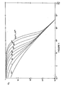
- the graph in Figure 1 characterizes the behavior of a homogeneous reservoir model and a well exhibiting the wall effect and the effect of compression or decompression of the fluid in the well.
- the curves of FIG. 1 are characterized by three distinct parts: the left part of the graph corresponding to short times and being characteristic of the effect of decompression of the fluid from the well (this effect is most important at the opening of the valve) ; the right part of the graph corresponding to a pure radial flow from the reservoir and an intermediate part between the left and right parts corresponding to a transient flow regime between the two preceding limit flows.
- This intermediate flow is a function of the decompression effect of the fluid and of the wall effect.
- the curves tend towards an asymptote corresponding to a derivative equal to 1. Indeed, at the very beginning of the tests, the predominant phenomenon is the decompression effect of the well which is characterized by the equation:
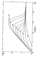
- the ordinate axis corresponds to P ' D ⁇ t D / C D and the abscissa axis corresponds to t D / C D' P ' D being the derivative of P with respect to t D / C D.
- Equation (7) can be written: It follows that for long times, the value of the product P ' D ⁇ t D / C D is equal to 0.5 and that the standard curves tend towards an asymptote of zero slope.
- FIG. 3 illustrates the use of the graph of the standard curves of FIG. 2. This graph has been reproduced in FIG.
- the value of the coefficient S of the wall effect is determined by the correspondence of the experimental curve with one of the standard curves, the correspondence of the two curves leading to the value of C D e 2S .
- the value of C D is determined by the value of C by the following equation: in which ⁇ c t h represents the porosity-compressibility-thickness product, known from geological studies (such as for example, analysis of samples or electrical logs) and r is the radius of the well.
- the value of the coefficient S can therefore be calculated from the value of C D e 2S .
- the standard curves represented in FIGS. 1 and 2 correspond to the behavior of a theoretical model of homogeneous formation when suddenly an increase in the flow rate of the fluid produced by the formation is imposed, and more especially when a valve is opened on the surface of the well to make it produce at constant flow while it was closed before ("drawdown" curve).
- the experimental curve is plotted on a logarithmic scale by plotting the time intervals A t on the abscissa and on the ordinate: tp representing the duration during which the training was put into production.
- the analysis of well tests can then be done by comparing this experimental curve with the standard curves of the graph in Figure 2.
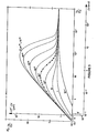
- FIG. 4 shows an example of application to a formation with double porosity.
- the fluid produced by the formation is contained in the matrix, that is to say in the rock composing the formation, and in the interstices or cracks contained in the matrix. There is therefore a system in which the fluid contained in the matrix first flows through the cracks before passing into the well.
- the coefficient w characterizes the ratio of the volume of fluid produced by the cracks to the volume of fluid produced by the total system (matrix + crack).
- the coefficient A characterizes the delay of the matrix to produce the fluid in the cracks compared to the production of the cracks themselves.
- the graph in Figure 4 corresponds to a theoretical training model with double porosity. On this graph, we have represented, in solid lines, the standard curves corresponding to the homogeneous model, identical to those of FIG. 2, in dotted lines of the standard curves by choosing as index and semi-dotted standard curves by choosing as index The dotted curves represent the equation: The semi-dotted curves represent the equation:
- a typical experimental curve characterizing a double porosity formation has also been represented by points.
- the use of the graph in FIG. 4 makes it possible to determine the values of the coefficients w and ⁇ , in addition to the values of kh, C and S. Note that the curves characterizing the behavior of a heterogeneous model have a very marked shape by applying the method according to the present invention.
- the present invention also makes it possible to plot on the same theoretical graph the standard curves of FIG. 2, P ' D ⁇ t D / C D as a function of t D / C D but also the standard curves P as a function of t D / C D described in United States Patent No. 4,328,705.
- the juxtaposition of these two series of standard curves on the same graph is shown in Figure 5.
- the method for determining the characteristics of an underground formation which has just been described has many advantages.
- the analysis of well tests can be carried out using a single graph, while the methods of the prior art call on a general graph on a logarithmic scale using all the experimental data and on a graph. specialized in semi-logarithmic scale and taking into account only part of the experimental data.
- the combination of the standard curves of the prior art with the standard curves of the present invention on the same graph has a certain advantage.
Landscapes
- Engineering & Computer Science (AREA)
- Mining & Mineral Resources (AREA)
- Geology (AREA)
- Life Sciences & Earth Sciences (AREA)
- Fluid Mechanics (AREA)
- Environmental & Geological Engineering (AREA)
- Chemical & Material Sciences (AREA)
- Physics & Mathematics (AREA)
- Analytical Chemistry (AREA)
- General Life Sciences & Earth Sciences (AREA)
- Geochemistry & Mineralogy (AREA)
- Geophysics And Detection Of Objects (AREA)
- Sampling And Sample Adjustment (AREA)
- Investigating Or Analysing Biological Materials (AREA)
- Testing Or Calibration Of Command Recording Devices (AREA)
Abstract
L'invention a pour objet une méthode de détermination des caractéristiques physiques d'un système formé d'un puits et d'une formation souterraine contenant un fluide et communiquant avec le puits. On provoque un changement de débit dudit fluide et on mesure une grandeur caractéristique de la pression P du fluide à des intervalles de temps successifs Δ t. On compare ensuite - d'une part, l'évolution théorique du logarithme de la dérivée P'D de la pression sans dimension en fonction du logarithme de tD/CD, la dérivée P'D étant par rapport à tD/CD, tD représentant le temps sans dimension et CD l'effet de compression ou de décompression du fluide dans le puits, avec - d'autre part, l'évolution expérimentale du logarithme de la dérivée Δ P' de la pression en fonction du logarithme des intervalles de temps correspondants Δ t, la dérivée Δ P' étant par rapport au temps t. On détermine enfin de la comparaison desdites évolutions théorique et expérimentale le produit kh de la perméabilité k par l'épaisseur de ladite formation h, et le coefficient C.The invention relates to a method for determining the physical characteristics of a system formed by a well and an underground formation containing a fluid and communicating with the well. A change in the flow rate of said fluid is caused and a quantity characteristic of the pressure P of the fluid is measured at successive time intervals Δ t. We then compare - on the one hand, the theoretical evolution of the logarithm of the derivative P'D of the dimensionless pressure as a function of the logarithm of tD / CD, the derivative P'D being with respect to tD / CD, tD representing dimensionless time and CD the compression or decompression effect of the fluid in the well, with - on the other hand, the experimental evolution of the logarithm of the derivative Δ P 'of the pressure as a function of the logarithm of the time intervals corresponding Δ t, the derivative Δ P 'being with respect to time t. Finally, from the comparison of said theoretical and experimental developments, the product kh of the permeability k is determined by the thickness of said formation h, and the coefficient C.
Description
La présente invention concerne les essais de puits d'hydrocarbures, permettant de déterminer les caractéristiques physiques du système formé d'un puits et d'une formation souterraine (appelée aussi "réservoir") produisant des hydrocarbures à travers le puits. De façon plus précise, l'invention se rapporte à une méthode selon laquelle le débit de fluide produit par le puits est modifié en fermant ou en ouvrant une vanne qui se trouve à la surface ou dans le puits. Les variations de pression résultantes sont mesurées et enregistrées au fond du puits en fonction du temps écoulé depuis le début des essais, c'est-à-dire depuis la modification du débit. Les caractéristiques du système puits-formation souterraine peuvent être déduites de ces données expérimentales. Les données expérimentales des essais de puits sont analysées en comparant la réponse de la formation souterraine à un changement de débit du fluide produit, avec le comportement de modèles théoriques ayant des caractéristiques bien définies et soumis au même changement de débit que la formation étudiée. Habituellement, les variations de pression en fonction du temps caractérisent le comportement du système puits-formation et l'enlèvement à débit constant de fluides, par l'ouverture d'une vanne dans le puits initialement fermé, est la condition d'essai qui est appliquée à la formation et au modèle théorique. Lorsque leurs comportements sont identiques, on suppose que le système étudié et le modèle théorique sont identiques aussi bien au point de vue quantitatif que qualitatif. En d'autres termes, ces réservoirs sont supposés avoir les mêmes caractéristiques physiques.The present invention relates to hydrocarbon well tests, making it possible to determine the physical characteristics of the system formed by a well and an underground formation (also called "reservoir") producing hydrocarbons through the well. More specifically, the invention relates to a method according to which the flow of fluid produced by the well is modified by closing or opening a valve which is located on the surface or in the well. The resulting pressure variations are measured and recorded at the bottom of the well as a function of the time elapsed since the start of the tests, that is to say since the modification of the flow rate. The characteristics of the underground well-formation system can be deduced from these experimental data. The experimental data from the well tests are analyzed by comparing the response of the underground formation to a change in the flow rate of the fluid produced, with the behavior of theoretical models having well-defined characteristics and subjected to the same change in flow rate as the formation studied. Usually, the variations of pressure as a function of time characterize the behavior of the well-formation system and the removal at constant flow rate of fluids, by the opening of a valve in the initially closed well, is the test condition which is applied to training and theoretical model. When their behaviors are identical, it is assumed that the system studied and the theoretical model are identical both quantitatively and qualitatively. In other words, these tanks are assumed to have the same physical characteristics.
Les caractéristiques obtenues de cette comparaison dépendent du modèle théorique : plus le modèle est compliqué, plus les caractéristiques qui peuvent être déterminées sont nombreuses. Le modèle de base est représenté par une formation homogène avec des limites supérieure et inférieure imperméables et avec une extension radiale infinie. Le débit dans la formation est alors radial, dirigé vers le puits.The characteristics obtained from this comparison depend on the theoretical model: the more complicated the model, the more numerous the characteristics that can be determined. The basic model is represented by a homogeneous formation with upper and lower limits impermeable and with infinite radial extension. The flow in the formation is then radial, directed towards the well.
Cependant, le modèle théorique le plus couramment utilisé est plus compliqué. Il comporte les caractéristiques du modèle de base auquel on ajoute des conditions internes telles que l'effet pariétal ("skin effect" en anglais) et l'effet de compression ou de décompression du fluide dans le puits ("wellbore storage" en anglais). L'effet pariétal est défini par un coefficient S qui caractérise l'endommagement ou la stimulation de la partie de la formation adjacente au puits. L'effet de compression ou de décompression du fluide dans le puits est caractérisé par un coefficient C qui résulte de la différence de débit de fluide produit par le puits, entre la formation souterraine et la tête de puits, lorsqu' une vanne située en tête de puits est soit fermée soit ouverte. Le coefficient C est exprimé habituellement en baril par psi, un baril étant égal à 0,16m3 et un psi égal à 0,069 bar.However, the most commonly used theoretical model is more complicated. It includes the characteristics of the basic model to which internal conditions are added such as the wall effect ("skin effect" in English) and the effect of compression or decompression of the fluid in the well ("wellbore storage" in English) . The wall effect is defined by a coefficient S which characterizes the damage or stimulation of the part of the formation adjacent to the well. The compression or decompression effect of the fluid in the well is characterized by a coefficient C which results from the difference in fluid flow produced by the well, between the underground formation and the wellhead, when a valve located at the head well is either closed or open. The coefficient C is usually expressed in barrels per psi, one barrel being equal to 0.16m 3 and one psi equal to 0.069 bar.
Le comportement d'un modèle théorique est représenté de façon commode par un graphe de courbes-type qui représentent les variations de pression, en fonction du temps, du fluide au fond du puits. Ces courbes sont habituellement tracées en coordonnées cartésiennes et en échelle logarithmique, la pression sans dimension étant portée en ordonnée et le temps sans dimension étant porté en abscisse. De plus, chaque courbe est caractérisée par un ou plusieurs nombres sans dimension qui représentent chacun une caractéristique (ou une combinaison de caractéristiques) du système théorique formé par un puits et un réservoir. Un paramètre sans dimension est défini par le paramètre réel (la pression par exemple) multiplié par une expression qui inclut certaines caractéristiques du système puits-réservoir de façon à rendre le paramètre sans dimension indépendant de ces caractéristiques.The behavior of a theoretical model is conveniently represented by a graph of standard curves which represent the pressure variations, as a function of time, of the fluid at the bottom of the well. These curves are usually plotted in Cartesian coordinates and on a logarithmic scale, the dimensionless pressure being plotted on the ordinate and dimensionless time being plotted on the abscissa. In addition, each curve is characterized by one or more dimensionless numbers which each represent a characteristic (or a combination of characteristics) of the theoretical system formed by a well and a reservoir. A dimensionless parameter is defined by the actual parameter (pressure for example) multiplied by an expression that includes certain characteristics of the well-reservoir system so as to make the dimensionless parameter independent of these characteristics.
C'est ainsi que le coefficient S caractérise uniquement l'effet pariétal mais est indépendant des autres caractéristiques du réservoir et des conditions expérimentales telles que le débit, la viscosité du fluide, la perméabilité de la formation, etc. Lorsque le modèle théorique et le système étudié puits-formation correspondent, la courbe expérimentale et l'une des courbe-types représentées avec les mêmes échelles de coordonnées ont une forme identique mais sont décalées l'une par rapport à l'autre. Les décalages suivant les deux axes, en ordonnée pour la pression et en abscisse pour le temps, sont proportionnels à des valeurs de caractéristiques du système puits-réservoir qui peuvent ainsi être déterminées.Thus the coefficient S characterizes only the wall effect but is independent of the other characteristics of the reservoir and experimental conditions such as the flow rate, the viscosity of the fluid, the permeability of the formation, etc. When the theoretical model and the well-formation system studied correspond, the experimental curve and one of the standard curves represented with the same coordinate scales have an identical shape but are offset with respect to each other. The offsets along the two axes, on the ordinate for pressure and on the abscissa for time, are proportional to the characteristic values of the well-reservoir system which can thus be determined.
Des informations qualitatives sur la formation souterraine, telle que par exemple la présence d'une fracture, sont obtenues par l'identification des différents régimes sur le graphe en échelle logarithmique représentant les données expérimentales. Sachant qu'une caractéristique particulière du système puits-réservoir, telle que par exemple une fracture verticale, se caractérise par un régime particulier, tous les différents régimes apparaissant sur le graphe des données expérimentales sont identifiées pour sélectionner le modèle de système puits-réservoir approprié. Des graphes spécialisés ne tenant compte que d'une partie des données expérimentales permettent la détermination plus précise des caractéristiques du système. On revient ensuite au graphe en échelle logarithmique prenant en compte toutes les données pour confirmer le choix du système et la détermination quantitative des caractéristiques de la formation. Ces dernières sont obtenues en sélectionnant une courbe-type ayant la même forme que la courbe expérimentale et en déterminant le décalage des axes de coordonnées de la courbe expérimentale par rapport à la courbe théorique.Qualitative information on the underground formation, such as for example the presence of a fracture, is obtained by the identification of the different regimes on the graph in logarithmic scale representing the experimental data. Knowing that a particular characteristic of the well-reservoir system, such as for example a vertical fracture, is characterized by a particular regime, all the different regimes appearing on the graph of the experimental data are identified in order to select the appropriate model of well-reservoir system. . Specialized graphs taking into account only part of the experimental data allow the more precise determination of the characteristics of the system. We then return to the graph on a logarithmic scale taking into account all the data to confirm the choice of the system and the quantitative determination of the characteristics of the training. The latter are obtained by selecting a standard curve having the same shape as the experimental curve and by determining the offset of the coordinate axes of the experimental curve with respect to the theoretical curve.
A un même modèle théorique correspondent plusieurs graphes de courbes- type. Ceci dépend des paramètres sans dimension choisis pour la représentation des axes de coordonnées du graphe, ainsi que d'un ou plusieurs "index". Un "index" n'est autre qu'un paramètre supplémentaire (ou une combinaison de paramètres)choisi pour la représentation des courbes, en complément des paramètres sans dimension des axes de coordonnées. La comparaison des différentes méthodes utilisées est donnée dans l'article intitulé "A Comparison Between Different Skin and Wellbore Storage Type Curves for Early-Time Transient Analysis" (Comparaison entre les différentes courbes-type avec effet pariétal et effet de compression ou de décompression pour l'analyse des transitoires précoces) par A.C. Gringarten & al., publié par "Society of Petroleum Engineers of AIME", (n2 SPE 8205). Le brevet des Etats-Unis d'Amérique 4,328,705 décrit également une méthode selon laquelle les courbes-type sont représentées en utilisant la pression sans dimension P pour l'axe des ordonnées et le rapport tD/CD pour l'axe des abscisses, tD étant le temps sans dimension et CD le coefficient sans dimension caractérisant l'effet de compression ou de décompression du fluide dans le puits. L'inconvénient de la méthode décrite dans ce brevet est que les courbes-type ont des formes variant relativement lentement l'une par rapport à l'autre. Il en résulte une certaine incertitude dans le choix de la courbe-type correspondant à la courbe expérimentale. On remarque également que pour effectuer une analyse complète, on est obligé de faire appel non seulement à un graphe en échelle logarithmique représentant l'ensemble des données expérimentales, mais d'utiliser également des graphes spécialisés, en échelle semi-logerithmique par exemple, pour n'analyser qu'une partie des données mais d'une façon plus précise.Several graphs of standard curves correspond to the same theoretical model. This depends on the dimensionless parameters chosen for the representation of the coordinate axes of the graph, as well as one or more "indexes". An "index" is nothing other than an additional parameter (or a combination of parameters) chosen for the representation of the curves, in addition to the dimensionless parameters of the coordinate axes. The comparison of the different methods used is given in the article entitled "A Comparison Between Different Skin and Wellbore Storage Type Curves for Early-Time Transient Analysis" (Comparison between the different standard curves with wall effect and compression or decompression effect for analysis of early transients) by AC Gringarten & al., published by "Society of Petroleum Engineers of AIME", (n 2 SPE 8205). The patent of the United States of America 4,328,705 also describes a method according to which the standard curves are represented using the dimensionless pressure P for the ordinate axis and the ratio t D / C D for the abscissa axis, t D being dimensionless time and C D dimensionless coefficient characterizing the effect of compression or decompression of the fluid in the well. The disadvantage of the method described in this patent is that the standard curves have shapes varying relatively slowly with respect to each other. This results in a certain uncertainty in the choice of the standard curve corresponding to the experimental curve. We also note that to perform a complete analysis, we are obliged not only to use a graph on a logarithmic scale representing all of the experimental data, but also to use specialized graphs, on a semi-logerithmic scale for example, to analyze only part of the data but in a more precise way.
3n a déjà songé à utiliser la dérivée mathématique de la pression sans dimension, P'D, au lieu de la pression sans dimension PD. C'est ainsi que dans l'article intitulé "Application of the P' Function to Interference Analysis" (Application de la fonction P'D à l'analyse des tests d'interférence) publié dans "Journal of Petroleum Technology" d'août 1980, page 1465, l'évolution de la dérivée P'D (dérivée par rapport à tD) en fonction de t est utilisée pour analyser des essais d'interférence entre un puits de production et un puits d'observation. On enregistre les variations de pression dans le puits d'observation lorsqu'on modifie le débit de fluide produit par le puits de production. Dans ce cas, l'effet pariétal et l'effet de compression ou de décompression du fluide n'interviennent pas. C'est donc un cas très simple dans lequel on analyse la réponse de la formation souterraine dans un puits éloigné du puits producteur. Il en résulte qu'il n'y a pas une famille de courbes-type mais une seule courbe.3n has already thought of using the mathematical derivative of dimensionless pressure, P ' D , instead of dimensionless pressure P D. Thus, in the article entitled "Implementation of the P 'Function to Interference Analysis" (Application of the function P' D in the analysis of interference tests) published in "Journal of Petroleum Technology" August 1980, page 1465, the evolution of the derivative P ' D (derivative with respect to t D ) as a function of t is used to analyze interference tests between a production well and an observation well. Pressure variations in the observation well are recorded when the fluid flow produced by the production well is changed. In this case, the parietal effect and the effect of compression or decompression of the fluid do not intervene. It is therefore a very simple case in which the response of the underground formation in a well distant from the producing well is analyzed. As a result, there is not a family of standard curves but a single curve.
La dérivée de la pression P'D (dérivée par rapport à tD) a été également mise à profit pour caractériser les réservoirs )contenant deux failles étanches parallèles autour du réservoir, dans l'article intitulé "Detection and Location of Two Parallel Sealing Faults Around a Well" (Détection et localisation de deux failles étanches parallèles autour d'un puits) paru dans "Journal of Petroleum Technology" d'octobre 1980, page 1701. Cet article 5ne traite que d'un problème particulier.The derivative of the pressure P ' D (derivative with respect to t D ) was also used to characterize the reservoirs) containing two parallel tight faults around the reservoir, in the article entitled "Detection and Location of Two Parallel Sealing Faults Around a Well "published in" Journal of Petroleum Technology "of October 1980, page 1701. This article deals only with a particular problem.
Le comportement en pression d'un puits produisant un fluide légèrement compressible à travers un plan unique d'une fracture verticale dans un réservoir infini a été analysé à l'aide de la dérivée mathématique de la pression sans dimension P'D, (dérivée Dpar rapport à un temps sans dimension tDf) dans l'article intitulé "Application of P'D Function to Vertically Fractured Wells" (Application de la fonction P'D au puits fracturé verticalement) paru dans "Society of Petroleum Engineers" of AIME, SPE 11028, du 26-29 septembre 1982.The pressure behavior of a well producing a slightly compressible fluid through a single plane of a vertical fracture in an infinite reservoir was analyzed using the mathematical derivative of the dimensionless pressure P ' D , (derivative Dpar compared to a dimensionless time t Df) in the article entitled "Application of P 'D function to vertically fractured wells" (Application of the function P' D vertically fractured wells) appeared in "Society of Petroleum Engineers" of LOVE, SPE 11028, September 26-29, 1982.
Cet article ne concerne qu'un cas particulier dans lequel la courbe-type est unique et pour lequel les avantages de l'utilisation de la dérivée de la pression ne sont pas évidents par rapport aux méthodes classiques. De plus, l'effet pariétal et l'effet de compression ou de décompression du fluide n'interviennent pas.This article only relates to a particular case in which the standard curve is unique and for which the advantages of using the pressure derivative are not obvious compared to conventional methods. In addition, the parietal effect and the effect of compression or decompression of the fluid do not intervene.
La présente invention a pour objet une méthode de détermination des caractéristiques d'un système puits-réservoir permettant une meilleure identification entre le comportement expérimental du système analysé formé par le puits et la formation souterraine et le comportement d'un modèle théorique. Ce modèle est général, à savoir que la formation peut être homogène ou hétérogène et qu'il tient compte de l'effet pariétal et de l'effet de compression ou de décompression du fluide et éventuellement de la double porosité du réservoir et des fractures du puits. La méthode selon la présente invention permet une analyse globale et unique du comportement du système puits-réservoir, sans recourir à des analyses spécialisées. L'invention permet également l'analyse des données expérimentales lorsque la condition imposée au système est la fermeture du puits, grâce à un choix judicieux des paramètres. La méthode selon la présente invention peut également être avantageusement combinée à une méthode de l'art antérieur.The present invention relates to a method for determining the characteristics of a well-reservoir system allowing better identification between the experimental behavior of the analyzed system formed by the well and the underground formation and the behavior of a theoretical model. This model is general, namely that the formation can be homogeneous or heterogeneous and that it takes into account the wall effect and the effect of compression or decompression of the fluid and possibly the double porosity of the reservoir and fractures of the well. The method according to the present invention allows a global and unique analysis of the behavior of the well-reservoir system, without resorting to specialized analyzes. The invention also allows the analysis of experimental data when the condition imposed on the system is the closing of the well, thanks to a judicious choice of parameters. The method according to the present invention can also be advantageously combined with a method of the prior art.
De façon plus précise, la présente invention concerne une méthode de détermination des caractéristiques physiques d'un système formé d'un puits et d'une formation souterraine contenant un fluide et communiquant avec ledit puits, ladite formation présentant de l'effet pariétal et/ou le fluide se comprimant ou se décomprimant dans le puits et ladite formation étant homogène ou hétérogène. Selon la méthode, on provoque un changement de débit dudit fluide, on mesure une grandeur caractéristique de la pression P du fluide à des intervalles de temps successifs àt et on compare,
- - d'une part, à partir d'un modèle théorique de système de puits-réservoir, l'évolution théorique du logarithme de la dérivée P'D de la pression sans dimension en fonction du logarithme de tD/CD, ladite dérivée P'D étant par rapport à tD/CD, tD représentant le temps sans dimension et CD le coefficient sans dimension de l'effet de compression ou de décompression du fluide dans le puits, avec
- - d'autre part, l'évolution expérimentale du logarithme de la dérivée A P' de la pression en fonction du logarithme des intervalles de temps correspondants Δ t, ladite dérivée Δ P' étant par rapport au temps t,
et on détermine de la comparaison desdites évolutions théorique et expérimentale au moins une caractéristique du système puits-formation, choisie parmi le produit kh de la perméabilité k par l'épaisseur de ladite formation h, le coefficient CD et le coefficient S de l'effet pariétal.More specifically, the present invention relates to a method for determining the physical characteristics of a system formed by a well and an underground formation containing a fluid and communicating with said well, said formation having a parietal effect and / or the fluid compressing or decompressing in the well and said formation being homogeneous or heterogeneous. According to the method, a change in the flow rate of said fluid is caused, a quantity characteristic of the pressure P of the fluid is measured at successive time intervals t and we compare,
- - on the one hand, from a theoretical model of reservoir-well system, the theoretical evolution of the logarithm of the derivative P ' D of the dimensionless pressure as a function of the logarithm of t D / C D , said derivative P ' D being with respect to t D / C D , t D representing dimensionless time and C D the dimensionless coefficient of the effect of compression or decompression of the fluid in the well, with
- - on the other hand, the experimental evolution of the logarithm of the derivative AP 'of the pressure as a function of the logarithm of the corresponding time intervals Δ t, said derivative Δ P' being with respect to time t,
and at least one characteristic of the well-formation system, chosen from the product kh of the permeability k by the thickness of said formation h, the coefficient C D and the coefficient S of l 'is determined from the comparison of said theoretical and experimental developments. wall effect.
Ladite évolution théorique peut avantageusement être celle du logarithme du produit P'D·tD/CD en fonction du logarithme de tD/CD et ladite évolution expérimentale est celle du logarithme du produit Δ P'. Δt en fonction du logarithme de Δt.Said theoretical evolution can advantageously be that of the logarithm of the product P ' D · t D / C D as a function of the logarithm of t D / C D and said experimental evolution is that of the logarithm of the product Δ P'. Δt as a function of the logarithm of Δt.
Ladite évolution théorique peut également être fonction d'un index représentant une grandeur caractéristique du produit CDe2S. Lorsque le changement de débit du fluide correspond à la fermeture du puits, on peut avantageusement comparer ladite évolution théorique avec l'évolution expérimentale du logarithme de l'expression :
On peut également tracer une courbe expérimentale à l'aide des données expérimentales avec la même échelle logarithmique que ledit graphe théorique, la courbe expérimentale représentant soit l'évolution expérimentale de A P' en fonction de At, soit l'évolution expérimentale du produit A P'. Δt en fonction de Δt. On peut alors faire correspondre la courbe expérimentale avec l'une des courbes-type du graphe théorique et on peut en déterminer certaines caractéristiques physiques du système puits-formation souterraine.One can also draw an experimental curve using experimental data with the same logarithmic scale as said theoretical graph, the experimental curve representing either the experimental evolution of AP 'as a function of At, or the experimental evolution of the product A P '. Δt as a function of Δt. We can then make the experimental curve correspond with one of the standard curves of the theoretical graph and we can determine certain physical characteristics of the underground well-formation system.
L'invention a également pour objet les graphes théoriques obtenus tel qu'indiqué précédemment.The subject of the invention is also the theoretical graphs obtained as indicated above.
L'invention sera mieux comprise à l'aide de la description qui va suivre de modes de réalisation de l'invention donnés à titre d'exemples explicatifs mais nullement limitatifs. La description se rapporte aux dessins qui l'accompagnent dans lesquels :
- - la figure 1 représente en échelle logarithmique un graphe de courbe-type représentant P'D en fonction de tD/CD2 l'index représentant les valeurs de CDe2S;
- - la figure 2 montre un graphe de courbes-type en échelle logarithmique représentant P'D·tD/CD en fonction de tD/CD, l'index étant CDe2S;
- - la figure 3 illustre la méthode selon la présente invention pour la détermination des caractéristiques physiques d'une formation souterraine produisant un fluide ;
- la figure 4 représente en échelle logarithmique un graphe de courbes-type représentant P'D.tD/CD en fonction de tD/C D pour une formation souterraine à double porosité ; et
- - la figure 5 représente deux séries de courbes-type en échelle logarithmique, l'une montrant des courbes-type connues et l'autre montrant des courbes-types selon la présente invention.
- - Figure 1 shows on a logarithmic scale a graph of standard curve representing P ' D as a function of t D / C D2 the index representing the values of C D e 2S ;
- - Figure 2 shows a graph of standard curves on a logarithmic scale representing P ' D · t D / C D as a function of t D / C D , the index being C D e 2S ;
- - Figure 3 illustrates the method according to the present invention for determining the physical characteristics of an underground formation producing a fluid;
- FIG. 4 represents on a logarithmic scale a graph of standard curves representing P ' D .t D / C D as a function of t D / C D for an underground formation with double porosity; and
- - Figure 5 shows two series of standard curves on a logarithmic scale, one showing known standard curves and the other showing standard curves according to the present invention.
Avant de mettre un puits d'hydrocarbures en production, on effectue généralement des mesures de façon à déterminer les caractéristiques physiques de la formation souterraine produisant ces hydrocarbures. Cette étape préliminaire avant la production est très importante car elle permet de définir les conditions les plus appropriées pour produire ces hydrocarbures et éventuellement pour améliorer la production. L'une de ces mesures consiste à faire varier le débit du fluide produit, en ouvrant ou fermant une vanne placée en tête de puits ou dans le puits lui-même, et à enregistrer les variations résultantes de pression en fonction du temps écoulé à partir de la modification de débit du fluide produit. On peut par exemple fermer complètement le puits et enregistrer l'augmentation de pression résultante (on obtiendra alors une courbe expérimentale dite courbe de "build-up"). On peut aussi faire produire un puits dont la production avait été arrêtée et enregistrer la diminution de pression correspondante (la courbe expérimentale obtenue s'appelle alors "courbe de drawdown").Before putting a hydrocarbon well into production, measurements are generally made in order to determine the physical characteristics of the underground formation producing these hydrocarbons. This preliminary stage before production is very important because it makes it possible to define the most appropriate conditions to produce these hydrocarbons and possibly to improve production. One of these measures consists in varying the flow rate of the fluid produced, by opening or closing a valve placed at the well head or in the well itself, and recording the resulting variations in pressure as a function of the time elapsed from the change in flow rate of the fluid produced. We can for example completely close the well and record the resulting pressure increase (we will then obtain an experimental curve called "build-up" curve). It is also possible to produce a well whose production had been stopped and record the corresponding reduction in pressure (the experimental curve obtained is then called "drawdown curve").
Les variations de pression en fonction du temps peuvent être suivies à l'aide d'une sonde descendue dans le puits à l'extrémité d'un câble. Le câble peut être électrique et dans ce cas transmettre les informations de pression directement à un enregistreur situé à la surface. Lorsque le câble n'est pas conducteur, les variations de pression sont enregistrées dans des mémoires disposées dans la sonde. Ces mémoires sont ensuite lues en surface. On peut également installer une jauge de pression dans une poche latérale de la colonne de production du puits, à proximité de la formation productrice. Un câble conducteur situé dans l'espace annulaire compris entre la colonne de production et le tubage relie la jauge de pression jusqu'à un enregistreur situé à la surface. Un tel dispositif est décrit par exemple dans les brevets des Etats-Unis n° 3,939,705 et 4,105,279.Pressure variations as a function of time can be monitored using a probe lowered into the well at the end of a cable. The cable can be electric and in this case transmit the pressure information directly to a recorder located on the surface. When the cable is not conductive, the pressure variations are recorded in memories located in the probe. These memories are then read on the surface. You can also install a pressure gauge in a side pocket of the production column of the well, near the producing formation. A conductive cable located in the annular space between the production column and the casing connects the pressure gauge to a recorder located on the surface. Such a device is described, for example, in United States patents 3,939,705 and 4,105,279.
Les valeurs mesurées par les sondes de pression ne correspondent généralement pas à la pression elle-même, mais à une grandeur caractéristique de la pression telle que, par exemple, une différence de deux fréquences. Par la suite, on utilisera l'expression "valeur de la pression" par commodité et clarté, tout en gardant à l'esprit que les données expérimentales peuvent correspondre à une grandeur caractéristique de la pression.The values measured by the pressure probes generally do not correspond to the pressure itself, but to a quantity characteristic of the pressure such as, for example, a difference of two frequencies. Thereafter, the expression "pressure value" will be used for convenience and clarity, while bearing in mind that the experimental data may correspond to a quantity characteristic of the pressure.
La figure 1 représente un graphe de nouvelles courbes-type, en échelle logarithmique, représentant la dérivée mathématique P'D de la pression sans dimension PD en fonction du rapport tD/CD t représente le temps sans dimension et CD représentant la valeur du coefficient sans dimension de l'effet de compression ou de décompression du fluide dans le puits. La dérivée mathématique P'D est faite par rapport à tD/CD. De plus, les variations de la dérivée de la pression P'D sont représentées par rapport à un index CDe2S, qui n'est autre qu'une combinaison de deux caractéristiques physiques C et S du système puits-réservoir analysé. Il est à remarquer que l'index CDe2S peut prendre une valeur quelconque, qui n'est pas nécessairement entière. La valeur de la pression sans dimension PD est donnée par l'équation suivante, en employant le système d'unités utilisé couramment dans l'industrie pétrolière et appelé "Oil field units" page 185 du livre intitulé "Advances in Well Test Analysis" publié par "Society of Petroleum Engineers of AIME" - 1977 :
- k représente la perméabilité de la formation souterraine,
- h est l'épaisseur de la formation,
- A P est la variation de pression,
- q est le débit du fluide en surface,
- B est le coefficient de dilatation du fluide entre le réservoir et la surface (appelé en anglais "formation volume factor") et
- µ est la viscosité du fluide.
- k represents the permeability of the underground formation,
- h is the thickness of the formation,
- AP is the pressure variation,
- q is the flow rate of the surface fluid,
- B is the coefficient of expansion of the fluid between the reservoir and the surface (called in English "formation volume factor") and
- µ is the viscosity of the fluid.
La dérivée mathématique P'D de la pression sans dimension PD, par rapport à tD/CD, est donnée par l'équation suivante :
La valeur du rapport tD/CD, dans le même système d'unités que pour les équations précédentes, est donnée par :
Le graphe de la figure 1 caractérise le comportement d'un modèle de réservoir homogène et d'un puits présentant l'effet pariétal et l'effet de compression ou de décompression du fluide dans le puits.The graph in Figure 1 characterizes the behavior of a homogeneous reservoir model and a well exhibiting the wall effect and the effect of compression or decompression of the fluid in the well.
Ce graphe est obtenue à partir de l'équation (A.2) de l'article intitulé "Determination of fissure volume and block size in fractured reservoirs by type-curve analysis" (Détermination du volume des fissures et de la taille des blocs dans les réservoirs fissurés par analyse par courbes-type) publié par "Society of Petroleum Engineers" en septembre 1980, n° SPE 9293. Cette équation est donnée dans le domaine de Laplace. L'inversion dans le domaine des temps réels est obtenue à l'aide d'un algorithme d'inversion, tel que celui décrit par exemple par H. Stehfest dans "Communications of the ACM, D-5" du 13.01.70, n°1 page 47.This graph is obtained from equation (A.2) of the article entitled "Determination of fissure volume and block size in fractured reservoirs by type-curve analysis "published by" Society of Petroleum Engineers "in September 1980, n ° SPE 9293. This equation is given in the Laplace domain. The inversion in the real time domain is obtained using an inversion algorithm, such as that described for example by H. Stehfest in "Communications of the ACM, D- 5 "of 13.01.70, n ° 1 page 47.
Les courbes de la figure 1 se caractérisent par trois parties distinctes : la partie gauche du graphe correspondant aux temps courts et étant caractéristique de l'effet de décompression du fluide du puits (cet effet est le plus important à l'ouverture de la vanne) ; la partie droite du graphe correspondant à un écoulement pur radial du réservoir et une partie intermédiaire entre les parties gauche et droite correspondant à un régime d'écoulement transitoire entre les deux écoulements-limite précédents. Cet écoulement intermédiaire est fonction de l'effet de décompression du fluide et de l'effet pariétal. Sur la partie gauche du graphe, les courbes tendent vers une asymptote correspondant à une dérivée égale à 1. En effet, au tout début des essais, le phénomène prédominant est l'effet de décompression du puits lequel est caractérisé par l'équation :
La dérivée de la pression sans dimension par rapport à tD/CD peut s'écrire :
On voit que la dérivée P'D, pour ce type d'écoulement est égal à 1 et que les courbes-type se réduisent à une droite de pente nulle. La partie droite du graphe de la figure 1, qui correspond à un écoulement radial infini dans une formation homogène, est caractérisée par l'équation :
En dérivant PD par rapport à tD/CD, on obtient :

On remarque que la courbe représentée par l'équation (8) est une droite de pente égale à -1. Pour les temps courts et les temps longs, les courbes sont rectilignes et indépendantes de CDe2S, ce qui est un avantage considérable par rapport aux méthodes de l'art antérieur. Entre les deux asymptotes, pour les temps intermédiaires, chaque courbe d'index Ce 2S a une forme différente bien contrastée.Note that the curve represented by equation (8) is a straight line with a slope equal to -1. For short times and long times, the curves are rectilinear and independent of C D e 2S , which is a considerable advantage compared to the methods of the prior art. Between the two asymptotes, for the intermediate times, each Ce 2S index curve has a different, well-contrasted shape.
Si dP représente la différence de deux mesures successives de la pression du fluide dans le puits et si dt représente l'intervalle de temps (court) séparant ces deux mesures successives, on calcule pour tous les couples de mesures successives les valeurs Δ P' = dP/dt. Ce calcul permet de déterminer de façon pratique Les valeurs successives de la dérivée mathématique ΔP' qui par léfinition est égale au rapport dP/dt lorsque dt tend vers zéro.En traçant la courbe Δ P' en fonction de At (Δ t étant L'intervalle de temps entre l'instant de la mesure considérée et L'instant de modification de débit du fluide) de façon à former un graphe expérimental, et en prenant les mêmes échelles logarithmiques que celles adoptées pour tracer les courbes-type de la figure 1, on peut déterminer les caractéristiques physiques du système puits-formation souterraine. En effet, le décalage des ordonnées de la courbe expérimentale et des courbes-type permet de déterminer la valeur de C (ce qui est évident au vu de l'équation (2), en effectuant log P'D-log Δ P' et en connaissant les valeurs de q et B). Le décalage des abscisses de la courbe expérimentale par rapport à la courbe-type choisie permet de déterminer la valeur kh (connaissant C et p, ce qui est évident au vu de l'équation (3) en effectuant logtD/CD - log At). Enfin le choix de la courbe-type correspondant à la courbe expérimentale permet de déterminer le coefficient S (par le calcul préalable de CD à partir de l'équation (14) comme il sera montré par la suite). Le graphe théorique de la figure 1 étant utilisé de la même façon que celui de la figure 2, par comparaison avec la courbe expérimentale, seule l'utilisation du graphe de la figure 2 est illustrée(figure 3).If dP represents the difference of two successive measurements of the pressure of the fluid in the well and if dt represents the time interval (short) separating these two successive measurements, we calculates for all the successive measurement pairs the values Δ P '= dP / dt. This calculation makes it possible to determine in a practical manner The successive values of the mathematical derivative ΔP 'which by definition is equal to the ratio dP / dt when dt tends towards zero. By plotting the curve Δ P' as a function of At (Δ t being L ' time interval between the instant of the measurement considered and the instant of modification of the flow rate of the fluid) so as to form an experimental graph, and by taking the same logarithmic scales as those adopted to plot the standard curves of FIG. 1 , we can determine the physical characteristics of the underground well-formation system. Indeed, the shift of the ordinates of the experimental curve and the standard curves makes it possible to determine the value of C (which is evident in the light of equation (2), by performing log P ' D -log Δ P' and knowing the values of q and B). The offset of the abscissae of the experimental curve with respect to the chosen standard curve makes it possible to determine the value kh (knowing C and p, which is obvious in view of equation (3) by performing logt D / C D - log At). Finally the choice of the standard curve corresponding to the experimental curve makes it possible to determine the coefficient S (by the prior calculation of C D from equation (14) as will be shown later). The theoretical graph of figure 1 being used in the same way as that of figure 2, by comparison with the experimental curve, only the use of the graph of figure 2 is illustrated (figure 3).
La méthode de détermination des caractéristiques physiques par utilisation du graphe de la figure 1 a été améliorée en suivant l'évolution, non plus de la dérivée mathématique de la pression sans dimension, mais en suivant l'évolution, en fonction de tD/CD, du produit de la dérivée P'D de la pression sans dimension (dérivée par rapport à tD/CD) par le rapport tD/CD. Cette nouvelle méthode est illustrée à la figure 2 par un graphe représentant le comportement d'une formation homogène présentant l'effet pariétal et l'effet de décompression du fluide du puits. L'axe des ordonnées correspond à P'D·tD/CD et l'axe des abscisses correspond à tD/CD' P'D étant la dérivée de P par rapport à tD/CD.The method of determining physical characteristics using the graph in Figure 1 has been improved by following the evolution, no longer of the mathematical derivative of the dimensionless pressure, but by following the evolution, as a function of t D / C D , of the product of the derivative P ' D of the dimensionless pressure (derivative with respect to t D / C D ) by the ratio t D / C D. This new method is illustrated in Figure 2 by a graph representing the behavior of a homogeneous formation presenting the wall effect and the decompression effect of the fluid in the well. The ordinate axis corresponds to P ' D · t D / C D and the abscissa axis corresponds to t D / C D' P ' D being the derivative of P with respect to t D / C D.
De plus, l'index CDe2S a été choisi pour représenter les courbes-type. Comme dans le cas de la figure 1, l'effet prédominant au début de l'essai de puits est l'effet de décompression du fluide. Cet effet correspond aux équations (4) et (5). A partir de l'équation (5), on peut écrire :In addition, the index C D e 2S was chosen to represent the standard curves. As in the case of Figure 1, the predominant effect at the start of the well test is the decompression effect of the fluid. This effect corresponds to equations (4) and (5). From equation (5), we can write:
![]()
![]()
Pour les temps longs, correspondant à la partie droite du graphe de la figure 2, les équations (6) et (7) demeurent valables puisqu'on se trouve en fin de test en écoulement radial infini pour une formation homogène. L'équation (7) peut s'écrire :
On remarque que pour le régime d'écoulement intermédiaire situé au centre du graphe de la figure 2, les courbes-type sont de forme très contrastée, ce qui permet une identification beaucoup plus précise de la courbe expérimentale avec l'une des courbes-type que par les méthodes de l'art antérieur. Par rapport au graphe de la figure 1, on peut dire que le graphe de la figure 2 correspond, en première approximation, à une rotation de 45° du graphe de la figure 1. Cependant, les courbes-type ont un relief plus accentué et la présentation du graphe de la figure 2 est plus pratique.Les valeurs de l'index CDe2S sont indiquées sur les courbes-type. La figure 3 illustre l'utilisation du graphe des courbes-type de la figure 2. Ce graphe a été reproduit sur la figure 3 avec, en ordonnée, P'D·tD/CD et en abscisse tD/CD. Les différences de pression dP mesurées dans le puits, pour des différences de temps successifs dt, sont utilisées pour calculer les valeurs Δ P' = dP/dt comme indiqué précédemment. On multiplie les valeurs successives de ΔP' par les intervalles de temps correspondants A t et on trace ensuite un graphe expérimental représentant le produit ΔP'. Δ t en ordonnée en fonction de A t en abscisse. Les valeurs de ΔP sont en psi (1 psi = 0,068 bar) et les valeurs de Δ t sont en heure. Les deux graphes théorique et expérimental ont la même échelle logarithmique. On commence par superposer la partie droite, qui est rectiligne, de la courbe expérimentale tracée sur la figure 3 à l'aide de points, à la partie rectiligne des courbes-type à droite du graphe. Ceci est facile à réaliser puisque cette partie des courbes est une droite de pente nulle. On décale ensuite le graphe expérimental le long de l'axe des temps de façon à faire correspondre sa partie gauche avec la partie gauche des courbes-type. Ceci est également facile puisque cette partie des courbes-type est une droite de pente égale à 1. Si la formation souterraine étudiée a un comportement homogène, la courbe expérimentale doit alors se superposer parfaitement, aux erreurs de précision des mesures près, a une courbe-type. Dans l'exemple montré sur la figure 3, cette courbe-type correspond à CDe2S = 1010. Le décalage des axes de coordonnées de la courbe expérimentale avec les axes des courbes-type permet de déterminer les valeurs du produit kh et la valeur de l'effet de décompression du fluide dans le puits. En effet, en combinant les équations (2) et (3),on obtient :

Le membre de gauche de cette dernière équation correspond au décalage des ordonnées représenté par Y sur la figure 3. La valeur de Y permet de déterminer le produit kh. En effet, la valeur du débit de fluide q est généralement connue par des mesures ayant été préalablement effectuées avec un débitmètre ou un séparateur, et les valeurs du coefficient B de dilatation du fluide et de sa viscosité p sont déterminées par l'analyse d'échantillons du fluide (analyse appelée habituellement "PVT"). En conséquence, la valeur du produit perméabilité - épaisseur kh peut être déterminée en connaissant la valeur Y mesurée. De la même façon, l'équation (3) peut s'écrire
Le membre de gauche de cette équation correspond au décalage X des abscisses de la courbe-type choisi et de la courbe expérimentale. Connaissant la valeur de ce décalage X ainsi que les valeurs de la viscosité p et du produit kh, on déduit de l'équation (13) la valeur du coefficient C de l'effet de décompression du fluide du puits.The left-hand side of this equation corresponds to the offset X of the abscissa of the chosen standard curve and of the experimental curve. Knowing the value of this offset X as well as the values of the viscosity p and of the product kh, we deduce from equation (13) the value of the coefficient C of the decompression effect of the fluid in the well.
La valeur du coefficient S de l'effet pariétal est déterminé par la correspondance de la courbe expérimentale avec l'une des courbes-type, la correspondance des deux courbes conduisant à la valeur de CDe2S. La valeur de CD est déterminée par la valeur de C par l'équation suivante :
Les courbes-type représentées sur les figures 1 et 2 correspondent au comportement d'un modèle théorique de formation homogène lorsqu'on impose soudainement une augmentation du débit du fluide produit par la formation, et plus spécialement lorsqu'on ouvre une vanne en surface du puits pour le faire produire à débit constant alors qu'il était fermé auparavant (courbe de "drawdown").The standard curves represented in FIGS. 1 and 2 correspond to the behavior of a theoretical model of homogeneous formation when suddenly an increase in the flow rate of the fluid produced by the formation is imposed, and more especially when a valve is opened on the surface of the well to make it produce at constant flow while it was closed before ("drawdown" curve).
Selon l'une des caractéristiques de la présente invention, pour les analyses d'essais de puits correspondant à la fermeture du puits, la courbe expérimentale est tracée en échelle logarithmique en portant en abscisse les intervalles de temps A t et en ordonnée :
La représentation des courbes-type, avec en ordonnée P'D·tD/CD et en abscisse t /C , est utilisable non seulement pour les formations souterraines homogènes mais également pour les formations non homogènes présentant par exemple une double porosité. La figure 4 montre un exemple d'application à une formation ayant une double porosité. Dans ce cas ,le fluide produit par la formation est contenu dans la matrice, c'est-à-dire dans la roche composant la formation, et dans les interstices ou fissures contenues dans la matrice. On a donc un système dans lequel le fluide, contenu dans la matrice s'écoule d'abord dans les fissures avant de passer dans le puits. Le coefficient w caractérise le rapport du volume de fluide produit par les fissures au volume de fluide produit par le système total (matrice + fissure). Le coefficient À caractérise le retard de la matrice à produire le fluide dans les fissures par rapport à la production des fissures elles-mêmes. Le graphe de la figure 4 correspond à un modèle théorique de formation ayant une double porosité. Sur ce graphe, on a représenté, en traits pleins, les courbes-type correspondant au modèle homogène, identiques à celles de la figure 2, en pointillés des courbes-type en choisissant comme index![]()
![]()


![]()
![]()
On a également représenté par des points une courbe expérimentale typique caractérisant une formation à double porosité. L'utilisation du graphe de la figure 4 permet de déterminer les valeurs des coefficients w et À , en plus des valeurs de kh, C et S. On remarque que les courbes caractérisant le comportement d'un modèle hétérogène ont une forme très marquée en appliquant la méthode selon la présente invention.A typical experimental curve characterizing a double porosity formation has also been represented by points. The use of the graph in FIG. 4 makes it possible to determine the values of the coefficients w and λ, in addition to the values of kh, C and S. Note that the curves characterizing the behavior of a heterogeneous model have a very marked shape by applying the method according to the present invention.
La présente invention permet également de tracer sur un même graphe théorique les courbes-type de la figure 2, P' D·tD/CD en fonction de tD/CD mais également les courbes-type P en fonction de tD/CD décrites dans le brevet des Etats-Unis d'Amérique n° 4,328,705. La juxtaposition de ces deux séries de courbes-type sur un même graphe est montrée sur la figure 5. On peut en effet réaliser cette superposition sur un même graphe car pour passer de P'D·tD/CD aux données expérimentales qui sont A P'. At, il faut multiplier ces dernières par un coefficient qui est donné par l'équation (11). Pour passer de P aux données expérimentales Δ P, dans le cas des courbes-type du brevet cité, il faut multiplier ces dernières par le même coefficient que précédemment. On peut donc superposer les deux séries de courbes-type et porter en ordonnée, avec une même échelle, PD et P'D·tD/CD. Pour utiliser le graphe théorique de la figure 5, on utilise alors un même graphe expérimental comportant deux courbes représentant en ordonnée les variations de pression Δ P pour l'une et Δ P'D·tD/CD pour l'autre, Δ t étant porté en abscisse pour les deux courbes. Le graphe combiné de la figure 5 permet une comparaison plus précise des deux courbes expérimentales avec les courbes-type.The present invention also makes it possible to plot on the same theoretical graph the standard curves of FIG. 2, P ' D · t D / C D as a function of t D / C D but also the standard curves P as a function of t D / C D described in United States Patent No. 4,328,705. The juxtaposition of these two series of standard curves on the same graph is shown in Figure 5. We can indeed achieve this superposition on the same graph because to move from P ' D · t D / C D to experimental data which are A P '. At, the latter must be multiplied by a coefficient which is given by equation (11). To go from P to the experimental data Δ P, in the case of the standard curves of the cited patent, it is necessary to multiply the latter by the same coefficient as above. We can therefore superimpose the two series of standard curves and carry on the ordinate, with the same scale, P D and P ' D · t D / C D. To use the theoretical graph in FIG. 5, we then use the same experimental graph comprising two curves representing on the ordinate the pressure variations Δ P for one and Δ P ' D · t D / C D for the other, Δ t being plotted on the abscissa for the two curves. The combined graph in Figure 5 allows a more precise comparison of the two experimental curves with the standard curves.
La méthode de détermination des caractéristiques d'une formation souterraine qui vient d'être décrite présente de nombreux avantages. Ainsi, l'analyse des essais de puits peut être effectuée à l'aide d'un seul graphe, alors que les méthodes de l'art antérieur font appel à un graphe général en échelle logarithmique en utilisant toutes les données expérimentales et à un graphe spécialisé en échelle semi-logarithmique et ne prenant en compte qu'une partie des données expérimentales. Du fait du comportement des modèles de systèmes formation-puits au début et en fin d'un essai de puits (temps courts et temps longs sur les graphes) qui se traduit par des lignes droites de pentes bien définies pour les deux extrémités des courbes-type ,le calage de la courbe expérimentale avec les courbes-type peut se faire sans ambiguïté. La combinaison des courbes-type de l'art antérieur avec les courbes-type de la présente invention sur un même graphe présente un avantage certain. De plus, la définition d'un nouveau temps, donné par l'équation (15), permet d'analyser les essais de puits effectués par la fermeture du puits. Il va sans dire que la présente invention ne se limite pas aux seuls modes de réalisation qui ont été décrits à titre d'exemples explicatifs mais nullement limitatifs. Ainsi, l'évolution des valeurs de pression ou de la dérivée des valeurs mesurées de pression peut être comparée à l'évolution théorique, calculée à partir d'un modèle de réservoir théorique, à l'aide de moyens informatiques tel qu'un ordinateur.The method for determining the characteristics of an underground formation which has just been described has many advantages. Thus, the analysis of well tests can be carried out using a single graph, while the methods of the prior art call on a general graph on a logarithmic scale using all the experimental data and on a graph. specialized in semi-logarithmic scale and taking into account only part of the experimental data. Due to the behavior of the well-formation system models at the start and at the end of a well test (short time and long time on the graphs) which results in straight lines of well defined slopes for the two ends of the standard curves, the calibration of the experimental curve with the standard curves can be unambiguous. The combination of the standard curves of the prior art with the standard curves of the present invention on the same graph has a certain advantage. In addition, the definition of a new time, given by equation (15), makes it possible to analyze the well tests carried out by the closure of the well. It goes without saying that the present invention is not limited to the sole embodiments which have been described by way of explanatory examples but in no way limitative. Thus, the evolution of the pressure values or the derivative of the measured pressure values can be compared to the theoretical evolution, calculated from a theoretical reservoir model, using computer means such as a computer. .
Claims (14)
et en ce que l'on détermine de la comparaison desdites évolutions théorique et expérimentale au moins une caractéristique du système puits-formation, choisie parmi le produit kh de la perméabilité k par l'épaisseur de ladite formation h, le coefficient C.1. Method for determining the physical characteristics of a system formed by a well and an underground formation containing a fluid and communicating with said well, said formation having a parietal effect and / or the fluid compressing or decompressing in the well and said formation being homogeneous or heterogeneous, method according to which a change in the flow rate of said fluid is measured and a quantity characteristic of the pressure P of the fluid is measured at successive time intervals Δt, said method being characterized in that l 'we compare,
and in that one determines from the comparison of said theoretical and experimental developments at least one characteristic of the well-formation system, chosen from the product kh of the permeability k by the thickness of said formation h, the coefficient C.

Applications Claiming Priority (2)
| Application Number | Priority Date | Filing Date | Title |
|---|---|---|---|
| FR8307075A FR2544790B1 (en) | 1983-04-22 | 1983-04-22 | METHOD FOR DETERMINING THE CHARACTERISTICS OF A SUBTERRANEAN FLUID-FORMING FORMATION |
| FR8307075 | 1983-04-22 |
Publications (2)
| Publication Number | Publication Date |
|---|---|
| EP0125164A1 true EP0125164A1 (en) | 1984-11-14 |
| EP0125164B1 EP0125164B1 (en) | 1986-12-30 |
Family
ID=9288354
Family Applications (1)
| Application Number | Title | Priority Date | Filing Date |
|---|---|---|---|
| EP84400781A Expired EP0125164B1 (en) | 1983-04-22 | 1984-04-19 | Method of determining the characteristics of an underground formation producing fluids |
Country Status (6)
| Country | Link |
|---|---|
| US (1) | US4597290A (en) |
| EP (1) | EP0125164B1 (en) |
| CA (1) | CA1209699A (en) |
| DE (1) | DE3461844D1 (en) |
| FR (1) | FR2544790B1 (en) |
| NO (1) | NO841473L (en) |
Cited By (4)
| Publication number | Priority date | Publication date | Assignee | Title |
|---|---|---|---|---|
| GB2161943A (en) * | 1984-07-19 | 1986-01-22 | Prad Res & Dev Nv | Method for estimating porosity and/or permeability |
| FR2573473A1 (en) * | 1984-11-20 | 1986-05-23 | Reijonen Veli Oy | METHOD FOR DETERMINING THE CAPACITY OF GROUNDWATER WELLS |
| US6832515B2 (en) | 2002-09-09 | 2004-12-21 | Schlumberger Technology Corporation | Method for measuring formation properties with a time-limited formation test |
| US7178392B2 (en) | 2003-08-20 | 2007-02-20 | Schlumberger Technology Corporation | Determining the pressure of formation fluid in earth formations surrounding a borehole |
Families Citing this family (36)
| Publication number | Priority date | Publication date | Assignee | Title |
|---|---|---|---|---|
| FR2569762B1 (en) * | 1984-08-29 | 1986-09-19 | Flopetrol Sa Etu Fabrications | HYDROCARBON WELL TEST PROCESS |
| FR2585404B1 (en) * | 1985-07-23 | 1988-03-18 | Flopetrol | METHOD FOR DETERMINING THE PARAMETERS OF FORMATIONS WITH MULTIPLE HYDROCARBON-PRODUCING LAYERS |
| EP0217684B1 (en) * | 1985-07-23 | 1993-09-15 | Flopetrol Services, Inc. | Process for measuring flow and determining the parameters of multilayer hydrocarbon-producing formations |
| EP0429078A1 (en) * | 1986-05-15 | 1991-05-29 | Soletanche | Method and apparatus for measuring ground permeability |
| US4797821A (en) * | 1987-04-02 | 1989-01-10 | Halliburton Company | Method of analyzing naturally fractured reservoirs |
| FR2613418B1 (en) * | 1987-04-02 | 1995-05-19 | Schlumberger Cie Dowell | MATRIX PROCESSING PROCESS IN THE OIL FIELD |
| US4843878A (en) * | 1988-09-22 | 1989-07-04 | Halliburton Logging Services, Inc. | Method and apparatus for instantaneously indicating permeability and horner plot slope relating to formation testing |
| US5050674A (en) * | 1990-05-07 | 1991-09-24 | Halliburton Company | Method for determining fracture closure pressure and fracture volume of a subsurface formation |
| US5005643A (en) * | 1990-05-11 | 1991-04-09 | Halliburton Company | Method of determining fracture parameters for heterogenous formations |
| US5517593A (en) * | 1990-10-01 | 1996-05-14 | John Nenniger | Control system for well stimulation apparatus with response time temperature rise used in determining heater control temperature setpoint |
| US5247829A (en) * | 1990-10-19 | 1993-09-28 | Schlumberger Technology Corporation | Method for individually characterizing the layers of a hydrocarbon subsurface reservoir |
| FR2710687B1 (en) * | 1993-09-30 | 1995-11-10 | Elf Aquitaine | Method for assessing the damage to the structure of a rock surrounding a well. |
| US5501273A (en) * | 1994-10-04 | 1996-03-26 | Amoco Corporation | Method for determining the reservoir properties of a solid carbonaceous subterranean formation |
| FR2747729B1 (en) * | 1996-04-23 | 1998-07-03 | Elf Aquitaine | METHOD FOR AUTOMATIC IDENTIFICATION OF THE NATURE OF A HYDROCARBON PRODUCTION WELL |
| US7031841B2 (en) * | 2004-01-30 | 2006-04-18 | Schlumberger Technology Corporation | Method for determining pressure of earth formations |
| ATE426732T1 (en) * | 2005-02-28 | 2009-04-15 | Schlumberger Technology Bv | METHOD FOR MEASURING FORMATION PROPERTIES USING A FORMATION TESTER |
| US7793718B2 (en) * | 2006-03-30 | 2010-09-14 | Schlumberger Technology Corporation | Communicating electrical energy with an electrical device in a well |
| US7735555B2 (en) * | 2006-03-30 | 2010-06-15 | Schlumberger Technology Corporation | Completion system having a sand control assembly, an inductive coupler, and a sensor proximate to the sand control assembly |
| US8056619B2 (en) | 2006-03-30 | 2011-11-15 | Schlumberger Technology Corporation | Aligning inductive couplers in a well |
| US7712524B2 (en) * | 2006-03-30 | 2010-05-11 | Schlumberger Technology Corporation | Measuring a characteristic of a well proximate a region to be gravel packed |
| US20080230221A1 (en) * | 2007-03-21 | 2008-09-25 | Schlumberger Technology Corporation | Methods and systems for monitoring near-wellbore and far-field reservoir properties using formation-embedded pressure sensors |
| US7580797B2 (en) * | 2007-07-31 | 2009-08-25 | Schlumberger Technology Corporation | Subsurface layer and reservoir parameter measurements |
| US8121790B2 (en) * | 2007-11-27 | 2012-02-21 | Schlumberger Technology Corporation | Combining reservoir modeling with downhole sensors and inductive coupling |
| US8136395B2 (en) | 2007-12-31 | 2012-03-20 | Schlumberger Technology Corporation | Systems and methods for well data analysis |
| US8078402B2 (en) * | 2008-07-16 | 2011-12-13 | Schlumberger Technology Corporation | Method of ranking geomarkers and compositional allocation of wellbore effluents |
| US20100147066A1 (en) * | 2008-12-16 | 2010-06-17 | Schlumberger Technology Coporation | Method of determining end member concentrations |
| US8839850B2 (en) * | 2009-10-07 | 2014-09-23 | Schlumberger Technology Corporation | Active integrated completion installation system and method |
| US20110192596A1 (en) * | 2010-02-07 | 2011-08-11 | Schlumberger Technology Corporation | Through tubing intelligent completion system and method with connection |
| US9249559B2 (en) | 2011-10-04 | 2016-02-02 | Schlumberger Technology Corporation | Providing equipment in lateral branches of a well |
| US9644476B2 (en) | 2012-01-23 | 2017-05-09 | Schlumberger Technology Corporation | Structures having cavities containing coupler portions |
| US9175560B2 (en) | 2012-01-26 | 2015-11-03 | Schlumberger Technology Corporation | Providing coupler portions along a structure |
| US9938823B2 (en) | 2012-02-15 | 2018-04-10 | Schlumberger Technology Corporation | Communicating power and data to a component in a well |
| US20130282286A1 (en) * | 2012-04-20 | 2013-10-24 | Chevron U.S.A. Inc. | System and method for calibrating permeability for use in reservoir modeling |
| US10036234B2 (en) | 2012-06-08 | 2018-07-31 | Schlumberger Technology Corporation | Lateral wellbore completion apparatus and method |
| GB2499523B (en) * | 2013-02-15 | 2014-04-09 | Petroleum Experts Ltd | Modelling of transient hydrocarbon reservoirs |
| CN114060018A (en) * | 2020-08-04 | 2022-02-18 | 中国石油天然气股份有限公司 | Reservoir dynamic reserve determining method, system, equipment and readable storage medium |
Citations (4)
| Publication number | Priority date | Publication date | Assignee | Title |
|---|---|---|---|---|
| US3550445A (en) * | 1968-01-19 | 1970-12-29 | Exxon Production Research Co | Method for testing wells for the existence of permeability damage |
| US3604256A (en) * | 1969-01-31 | 1971-09-14 | Shell Oil Co | Method for measuring the average vertical permeability of a subterranean earth formation |
| US3636762A (en) * | 1970-05-21 | 1972-01-25 | Shell Oil Co | Reservoir test |
| US4328705A (en) * | 1980-08-11 | 1982-05-11 | Schlumberger Technology Corporation | Method of determining characteristics of a fluid producing underground formation |
-
1983
- 1983-04-22 FR FR8307075A patent/FR2544790B1/en not_active Expired
-
1984
- 1984-04-04 CA CA000451272A patent/CA1209699A/en not_active Expired
- 1984-04-12 NO NO841473A patent/NO841473L/en unknown
- 1984-04-19 DE DE8484400781T patent/DE3461844D1/en not_active Expired
- 1984-04-19 EP EP84400781A patent/EP0125164B1/en not_active Expired
- 1984-04-19 US US06/601,838 patent/US4597290A/en not_active Expired - Fee Related
Patent Citations (4)
| Publication number | Priority date | Publication date | Assignee | Title |
|---|---|---|---|---|
| US3550445A (en) * | 1968-01-19 | 1970-12-29 | Exxon Production Research Co | Method for testing wells for the existence of permeability damage |
| US3604256A (en) * | 1969-01-31 | 1971-09-14 | Shell Oil Co | Method for measuring the average vertical permeability of a subterranean earth formation |
| US3636762A (en) * | 1970-05-21 | 1972-01-25 | Shell Oil Co | Reservoir test |
| US4328705A (en) * | 1980-08-11 | 1982-05-11 | Schlumberger Technology Corporation | Method of determining characteristics of a fluid producing underground formation |
Non-Patent Citations (1)
| Title |
|---|
| WORLD OIL, vol. 196, no. 6, mai 1983, pages 95-106, Houston, Texas, US; D. BOURDET et al.: "A new set of type curves simplifies well test analysis" * |
Cited By (10)
| Publication number | Priority date | Publication date | Assignee | Title |
|---|---|---|---|---|
| GB2161943A (en) * | 1984-07-19 | 1986-01-22 | Prad Res & Dev Nv | Method for estimating porosity and/or permeability |
| FR2573473A1 (en) * | 1984-11-20 | 1986-05-23 | Reijonen Veli Oy | METHOD FOR DETERMINING THE CAPACITY OF GROUNDWATER WELLS |
| GB2167471A (en) * | 1984-11-20 | 1986-05-29 | Veli E Reijonen | Ground water wells |
| US6832515B2 (en) | 2002-09-09 | 2004-12-21 | Schlumberger Technology Corporation | Method for measuring formation properties with a time-limited formation test |
| US7024930B2 (en) | 2002-09-09 | 2006-04-11 | Schlumberger Technology Corporation | Method for measuring formation properties with a time-limited formation test |
| US7036579B2 (en) | 2002-09-09 | 2006-05-02 | Schlumberger Technology Corporation | Method for measuring formation properties with a time-limited formation test |
| US7117734B2 (en) | 2002-09-09 | 2006-10-10 | Schlumberger Technology Corporation | Method for measuring formation properties with a time-limited formation test |
| US7210344B2 (en) | 2002-09-09 | 2007-05-01 | Schlumberger Technology Corporation | Method for measuring formation properties with a time-limited formation test |
| US7263880B2 (en) | 2002-09-09 | 2007-09-04 | Schlumberger Technology Corporation | Method for measuring formation properties with a time-limited formation test |
| US7178392B2 (en) | 2003-08-20 | 2007-02-20 | Schlumberger Technology Corporation | Determining the pressure of formation fluid in earth formations surrounding a borehole |
Also Published As
| Publication number | Publication date |
|---|---|
| DE3461844D1 (en) | 1987-02-05 |
| FR2544790B1 (en) | 1985-08-23 |
| FR2544790A1 (en) | 1984-10-26 |
| NO841473L (en) | 1984-10-23 |
| CA1209699A (en) | 1986-08-12 |
| EP0125164B1 (en) | 1986-12-30 |
| US4597290A (en) | 1986-07-01 |
Similar Documents
| Publication | Publication Date | Title |
|---|---|---|
| EP0125164B1 (en) | Method of determining the characteristics of an underground formation producing fluids | |
| EP0113285B1 (en) | Method and apparatus for determining the fluid flow characteristics in a bore hole by temperature measurement | |
| CN107701180B (en) | Original oil reservoir water saturation calculation method based on closed coring | |
| US5247830A (en) | Method for determining hydraulic properties of formations surrounding a borehole | |
| EP1963886B1 (en) | Method for quantitatively evaluating fluid pressures and for detecting excess pressures of an underground medium | |
| CA2517244A1 (en) | Method of determination of multiphase flow parameters for a porous medium, taking into account local heterogeneity | |
| CA2624305A1 (en) | Methods and systems for determining reservoir properties of subterranean formations | |
| EP1167948A1 (en) | Process for evaluating physical parameters of a subterranian reservoir starting from rock debris taken thereof | |
| Novakowski | Analysis of pulse interference tests | |
| WO2003098196A1 (en) | Method for evaluating capillary pressure curve of an underground deposit rocks based on rock cuttings measurements | |
| WO2006120366A1 (en) | Methods for analysis of pressure response in underground formations | |
| EP0174890B1 (en) | Method for hydrocarbon well testing | |
| EP2339485A1 (en) | Method of exploiting an oilfield by reconstructing the reservoir model | |
| FR3034191B1 (en) | DETERMINATION OF TRAINING PRESSURE | |
| FR3002270A1 (en) | METHOD FOR OPERATING A GEOLOGICAL TANK USING A STANDARD TANK MODEL AND COHERENT WITH RESPECT TO FLOW PROPERTIES | |
| FR3067750A1 (en) | QUANTIFICATION OF DOWNHOLE SAMPLE CONTAMINATION | |
| EP3626929A1 (en) | Method for operating a hydrocarbon reservoir by injecting a polymer | |
| EP2128653A2 (en) | Method for locating the spatial origin of a seismic event occurring within an underground formation | |
| EP2315055B1 (en) | Interpretation method for repetitive seismic data | |
| WO2009153443A1 (en) | Method for determining fluid pressures and for detecting overpressures in an underground medium | |
| CA2711926A1 (en) | Method, software and computer system for making a 3d geological mode | |
| FR2831917A1 (en) | METHOD FOR DETERMINING THE VARIATION IN PERMEABILITY RELATING TO AT LEAST ONE FLUID FROM A FLUID-CONTAINING TANK BASED ON THE SATURATION IN ONE OF THEM | |
| Banerjee et al. | A method for analysis of pressure response with a formation tester influenced by supercharging | |
| CA3066970A1 (en) | Improvements in or relating to injection wells | |
| FR3059033A1 (en) | VECTOR REPORTING SAFETY FACTOR FOR TUBULAR WELLBORE DESIGN |
Legal Events
| Date | Code | Title | Description |
|---|---|---|---|
| PUAI | Public reference made under article 153(3) epc to a published international application that has entered the european phase |
Free format text: ORIGINAL CODE: 0009012 |
|
| AK | Designated contracting states |
Designated state(s): DE GB IT NL |
|
| 17P | Request for examination filed |
Effective date: 19850214 |
|
| 17Q | First examination report despatched |
Effective date: 19860220 |
|
| GRAA | (expected) grant |
Free format text: ORIGINAL CODE: 0009210 |
|
| AK | Designated contracting states |
Kind code of ref document: B1 Designated state(s): DE GB IT NL |
|
| REF | Corresponds to: |
Ref document number: 3461844 Country of ref document: DE Date of ref document: 19870205 |
|
| ITF | It: translation for a ep patent filed |
Owner name: DOTT. FRANCO CICOGNA |
|
| PLBE | No opposition filed within time limit |
Free format text: ORIGINAL CODE: 0009261 |
|
| STAA | Information on the status of an ep patent application or granted ep patent |
Free format text: STATUS: NO OPPOSITION FILED WITHIN TIME LIMIT |
|
| 26N | No opposition filed | ||
| ITTA | It: last paid annual fee | ||
| PGFP | Annual fee paid to national office [announced via postgrant information from national office to epo] |
Ref country code: NL Payment date: 19910430 Year of fee payment: 8 |
|
| PGFP | Annual fee paid to national office [announced via postgrant information from national office to epo] |
Ref country code: DE Payment date: 19910529 Year of fee payment: 8 |
|
| PG25 | Lapsed in a contracting state [announced via postgrant information from national office to epo] |
Ref country code: NL Effective date: 19921101 |
|
| NLV4 | Nl: lapsed or anulled due to non-payment of the annual fee | ||
| PG25 | Lapsed in a contracting state [announced via postgrant information from national office to epo] |
Ref country code: DE Effective date: 19930101 |
|
| REG | Reference to a national code |
Ref country code: GB Ref legal event code: IF02 |
|
| PGFP | Annual fee paid to national office [announced via postgrant information from national office to epo] |
Ref country code: GB Payment date: 20020417 Year of fee payment: 19 |
|
| PG25 | Lapsed in a contracting state [announced via postgrant information from national office to epo] |
Ref country code: GB Free format text: LAPSE BECAUSE OF NON-PAYMENT OF DUE FEES Effective date: 20030419 |
|
| GBPC | Gb: european patent ceased through non-payment of renewal fee |
Effective date: 20030419 |