CN113826030A - Radiation detection with pulse pile-up nonparametric decomposition - Google Patents
Radiation detection with pulse pile-up nonparametric decomposition Download PDFInfo
- Publication number
- CN113826030A CN113826030A CN202080037871.4A CN202080037871A CN113826030A CN 113826030 A CN113826030 A CN 113826030A CN 202080037871 A CN202080037871 A CN 202080037871A CN 113826030 A CN113826030 A CN 113826030A
- Authority
- CN
- China
- Prior art keywords
- pulse
- statistics
- estimate
- noise
- mapping
- Prior art date
- Legal status (The legal status is an assumption and is not a legal conclusion. Google has not performed a legal analysis and makes no representation as to the accuracy of the status listed.)
- Pending
Links
Images


Classifications
-
- G—PHYSICS
- G01—MEASURING; TESTING
- G01T—MEASUREMENT OF NUCLEAR OR X-RADIATION
- G01T1/00—Measuring X-radiation, gamma radiation, corpuscular radiation, or cosmic radiation
- G01T1/16—Measuring radiation intensity
- G01T1/17—Circuit arrangements not adapted to a particular type of detector
- G01T1/171—Compensation of dead-time counting losses
-
- G—PHYSICS
- G01—MEASURING; TESTING
- G01R—MEASURING ELECTRIC VARIABLES; MEASURING MAGNETIC VARIABLES
- G01R23/00—Arrangements for measuring frequencies; Arrangements for analysing frequency spectra
- G01R23/02—Arrangements for measuring frequency, e.g. pulse repetition rate; Arrangements for measuring period of current or voltage
- G01R23/15—Indicating that frequency of pulses is either above or below a predetermined value or within or outside a predetermined range of values, by making use of non-linear or digital elements (indicating that pulse width is above or below a certain limit)
-
- G—PHYSICS
- G01—MEASURING; TESTING
- G01R—MEASURING ELECTRIC VARIABLES; MEASURING MAGNETIC VARIABLES
- G01R23/00—Arrangements for measuring frequencies; Arrangements for analysing frequency spectra
- G01R23/02—Arrangements for measuring frequency, e.g. pulse repetition rate; Arrangements for measuring period of current or voltage
-
- G—PHYSICS
- G01—MEASURING; TESTING
- G01R—MEASURING ELECTRIC VARIABLES; MEASURING MAGNETIC VARIABLES
- G01R23/00—Arrangements for measuring frequencies; Arrangements for analysing frequency spectra
- G01R23/16—Spectrum analysis; Fourier analysis
-
- G—PHYSICS
- G01—MEASURING; TESTING
- G01T—MEASUREMENT OF NUCLEAR OR X-RADIATION
- G01T1/00—Measuring X-radiation, gamma radiation, corpuscular radiation, or cosmic radiation
- G01T1/36—Measuring spectral distribution of X-rays or of nuclear radiation spectrometry
-
- G—PHYSICS
- G06—COMPUTING; CALCULATING OR COUNTING
- G06F—ELECTRIC DIGITAL DATA PROCESSING
- G06F17/00—Digital computing or data processing equipment or methods, specially adapted for specific functions
- G06F17/10—Complex mathematical operations
- G06F17/18—Complex mathematical operations for evaluating statistical data, e.g. average values, frequency distributions, probability functions, regression analysis
-
- G—PHYSICS
- G01—MEASURING; TESTING
- G01R—MEASURING ELECTRIC VARIABLES; MEASURING MAGNETIC VARIABLES
- G01R29/00—Arrangements for measuring or indicating electric quantities not covered by groups G01R19/00 - G01R27/00
- G01R29/02—Measuring characteristics of individual pulses, e.g. deviation from pulse flatness, rise time or duration
- G01R29/027—Indicating that a pulse characteristic is either above or below a predetermined value or within or beyond a predetermined range of values
- G01R29/033—Indicating that a pulse characteristic is either above or below a predetermined value or within or beyond a predetermined range of values giving an indication of the number of times this occurs, i.e. multi-channel analysers (the characteristic being frequency)
Landscapes
- Physics & Mathematics (AREA)
- General Physics & Mathematics (AREA)
- Spectroscopy & Molecular Physics (AREA)
- Life Sciences & Earth Sciences (AREA)
- Engineering & Computer Science (AREA)
- Health & Medical Sciences (AREA)
- High Energy & Nuclear Physics (AREA)
- Molecular Biology (AREA)
- Data Mining & Analysis (AREA)
- Mathematical Physics (AREA)
- Pure & Applied Mathematics (AREA)
- Theoretical Computer Science (AREA)
- Computational Mathematics (AREA)
- Mathematical Analysis (AREA)
- Mathematical Optimization (AREA)
- Nonlinear Science (AREA)
- Probability & Statistics with Applications (AREA)
- Bioinformatics & Cheminformatics (AREA)
- Operations Research (AREA)
- Algebra (AREA)
- Evolutionary Biology (AREA)
- Databases & Information Systems (AREA)
- Software Systems (AREA)
- General Engineering & Computer Science (AREA)
- Bioinformatics & Computational Biology (AREA)
- Measurement Of Radiation (AREA)
Abstract
A method of determining an energy spectrum of a single radiation quantum received in a radiation detector is disclosed. The spectral sensitivity statistics are computed from a time series of digital observations from the radiation detector, defining a mapping from pulse amplitude density to spectral sensitivity statistics. The energy spectrum is determined by applying the inverse of the mapping to the spectrum sensitive statistics to estimate the density of pulse amplitudes. The statistics may be based on: a first set of non-overlapping time intervals of constant length L irrespective of the entirety of the pulse cluster, the constant length L being at least as long as the duration of the pulses; and a second set of non-overlapping time intervals of constant length L1 less than L, also without regard to the entirety of the pulse cluster. A method of estimating a count rate is also disclosed.
Description
Technical Field
A novel method is provided for estimating the energy distribution of a radiation quantum, such as a photon incident on a detector in a spectroscopic system such as X-ray or gamma-ray spectroscopy. This method is particularly useful for count rate methods where pulse pile-up is an issue. The key step in deriving the estimator of embodiments of the present invention is to reformulate the problem novelty as a decomposition problem for the composite poisson process. The method may be applied to any form of radiation detector that detects quanta or other particles of radiation, such as x-rays, gamma rays or other photons, neutrons, atoms, molecules or seismic pulses. The use of spectroscopy from such detectors is well known. Such applications are widely described in the prior art, including in international patent applications PCT/AU2005/001423, PCT/AU2009/000393, PCT/AU2009/000394, PCT/AU2009/000395, PCT/AU2009/001648, PCT/AU2012/000678, PCT/AU2014/050420, PCT/AU2015/050752, PCT/AU2017/050514, and PCT/AU2017/050512, each of which is incorporated herein in its entirety for the purpose of describing potential applications of the current invention and understanding any other background material required by the current invention.
Background
X-ray and gamma-ray spectroscopy support a wide range of scientific, industrial and commercial processes. One goal of spectroscopy is to estimate the energy distribution of photons incident on a detector. From a signal processing point of view, the challenge is to convert the pulse stream output by the detector into a histogram of the area under each pulse. The pulses are generated from a poisson distribution, the ratio of which corresponds to the intensity of the X-rays or gamma-rays used to irradiate the sample. Increasing the intensity results in more pulses per second on average, and thus in acquisitionA shorter time before an accurate histogram is obtained. In applications such as airport baggage scanning, this translates directly into greater throughput. Pulse pile-up occurs when two or more pulses overlap in the time domain. As the count rate (average number of pulses per second) increases, the incidence of pulse pile-up also increases. This increases the difficulty in determining the number of pulses present and the area under each pulse. At the limit, the problem is pathological: if two pulses start at substantially the same time, their superposition cannot be distinguished from a single pulse. The response of an X-ray or gamma-ray detector to incident photons can be modeled as a pulse shape function Superposition of the convolution with Dirac-delta pulses,

time of arrival Unknown, and forms a poisson process. Each photon arrival is modeled as a time
 And has a dirac-delta of and proportional to photon energy and gives rise to a detector pulse shape response
 Amplitude of (2)
 . Amplitude of
 Is a function of its common probability density
 Unknown identityRandom variation of cloth
 The implementation of (1). Function of pulse shape
 Determined by the detector geometry and photon interactions. In some systems, the variation in pulse shape is minimal and negligible, while other systems (e.g., HPGe) the individual pulse shapes may differ significantly from each other [1]. Assuming that all pulse shapes are causal, i.e. for t< 0,
 Unimodal, finite energy, and follows
 But decays exponentially towards zero. The integral of the pulse shape function is normalized to unity, i.e.
 So that the area under the pulse is made of
 It is given. The observed signal consists of the detector output corrupted by noise, i.e.,

the mathematical goal of pulse pile-up correction is at a given time In the case of uniformly sampled, finite length versions of
 And (6) estimating. We always assume a noise distribution
 Is of known variance
 Zero mean gaussian distribution. We also assume that the photon arrival times form a homogeneous poisson process with a known ratio. Consisting of a detector response R corrupted by a noise process W, wherein
 、
、 And
And represents the second of each sequencekAn element, and wherein
 . LetS、RAndWare uniformly sampled time series corresponding to these signals,

wherein 。
。
The pulse processing method is summarized as follows: for decades, many approaches have been proposed to address the problem of pulse pile-up. Methods can be broadly classified into two types: time domain based and energy domain based. One popular strategy is to attempt to detect when pile-up occurs in the time domain and reject or compensate for the affected pulses. Early spectroscopic systems employed a rejection-based approach along with matched filtering. The disadvantage of this approach is that as the probability of pile-up increases, an increasing proportion of the pulses are rejected. The system falls into paralysis rapidly, setting an upper limit for the count rate [ 1]]. Compensating or correcting for stacked policy numbers with increased inexpensive computing powerThe amount has increased. These include template fitting [2 ]]Baseline subtraction [3]Adaptive filtering [4, 5 ]]Sparse regression [6, 7 ]]And the like. Both of these methods attempt to identify and compensate for pile-up in the time domain and are generally best suited for systems with low pulse shape variation. The complexity of these methods depends on the pulse shape The variability between them increases significantly. It can be shown that any method that attempts to characterize a single pulse will suffer from pile-up. The best these methods can do is to reduce the occurrence of stacking. Energy-based methods attempt to resolve the pile-up based on the statistics of a set of pulses rather than a single pulse. They typically operate on a histogram of the estimated energy (area under the pulse cluster). Early work on Wielopolski and Gardner [8]And a more recent expansion of their thoughts [9]Aggregation-based policies are mainly used in the energy domain to operate. Trigano et al [10, 11]]The incident spectrum is estimated using edge densities from a joint distribution of statistical properties of the variable length pulse clusters, where the beginning and end of each cluster is detected. This avoids the need to identify individual pulses and is robust to pulse shape variations. Ilhe et al [12 ]]The exponential shot noise process was examined to limit the pulse shape to a simple exponential to obtain an easy-to-handle result. Further work has been done [13]To allow a wider range of pulse shapes. In both cases, knowledge of the pulse shape is required, together with an estimation of the characteristic function and its derivatives.
Disclosure of Invention
We have chosen an energy-based pile-up correction method to i) avoid the limitations associated with single pulse detection [14]And ii) is able to handle pulse shape changes without unduly increasing computational complexity. We do not use joint distribution [10, 11]]Or a bulk process [ 12)]Instead, the stacking problem is recast as a "decomposition" problem of the composite poisson process. The composite Poisson process is a discrete-time random process in which each component consists of a sum of random numbers of independently identically distributed random variables, where the number of random variables in each sum is the number of Poisson's numbersDistributed [15]. The "decomposition" of the composite poisson process is the task of using a random sum to estimate the distribution from which random variables have been extracted. Buchmann and [16]the decomposition of the composite poisson process is set forth in the context of insurance claims and queuing theory. The decomposition of a uniformly sampled composite Poisson process has received some attention at the latest time [16, 17, 18, 12, 19]. These derived contexts often (reasonably) assume that each event is detectable (i.e., no ambiguity as to the number of events), or that the density estimator is conditioned on at least one event occurring in each observation [20 ]]. These assumptions are of limited value in solving the spectral stacking problem.
Unconditional non-parametric decomposition studies on event detection have received relatively little attention in the literature. Gugushvili [18] proposes a nonparametric, kernel-based estimator for the decomposition problem in the presence of Gaussian noise. In embodiments of the present invention, the inventors have envisaged that once the method for selecting the nuclear bandwidth is obtained, together with the method for transforming the observed detector outputs to fit the mathematical model, the estimator can be easily extended and applied to the reconstruction of the spectral pile-up problem.
According to a first broad aspect of the present invention, there is provided a method of determining the energy spectrum of a single radiation quantum received in a radiation detector, the method comprising the steps of: (1) obtaining a time series of digital observations from a radiation detector, the time series comprising pulses corresponding to the detection of individual quanta; (2) calculating a power spectrum sensitivity statistic from the detector signal, the power spectrum sensitivity statistic defining a mapping from pulse amplitude density to power spectrum sensitivity statistic; (3) the energy spectrum is determined by applying the inverse of the mapping to the spectrum sensitive statistics to estimate the density of pulse amplitudes.
In an embodiment, the energy spectrum sensitive statistics may be based on a sum of numerical observations over multiple time intervals, and the mapping may be defined using an approximate composite poisson process, which may be enhanced by modeling noise. The mapping may be expressed as a relationship between a characteristic function of amplitude, energy spectrum sensitive statistics, and modeled noise. The feature function of the spectrum sensitive statistics may be calculated by using a histogram of the sum of digital observations to which an inverse fourier transform is applied. The calculation of the characteristic function of the amplitude may comprise using a low-pass filter.
In a first embodiment, the plurality of time intervals are non-overlapping and have a constant length L, and each interval is selected to contain zero or more approximately complete clusters of pulses. This can be achieved by requiring a maximum value of the detector signal at the beginning and end of each time interval. In this embodiment, the composite poisson process may be defined as the sum of the pulse amplitudes in each time interval. The mapping may be expressed as defined in equations (40) and (41), which may be enhanced by a windowing function.
In a second embodiment, the plurality of intervals includes a first set of non-overlapping time intervals of constant length L that are selected without regard to the entirety of the pulse clusters, and a second set of non-overlapping time intervals of constant length L1 that are less than L that are also selected without regard to the entirety of the pulse clusters. L is at least as long as the duration of the pulse and preferably L1 is less than the duration of the pulse. In this embodiment, the composite poisson process may be as defined in section 6. The mapping may be expressed as defined in section 6. The second embodiment may utilize the processing and calculation for each set of time intervals as defined for the set of time intervals in the first embodiment.
In an embodiment, a data-driven strategy is used that results in a near-optimal selection of kernel parameters that minimizes the Integrated Squared Error (ISE) of the estimated probability density function of the incident photon energy.
According to a second broad aspect of the present invention, there is provided a method of estimating the individual radiation quantum count rates received in a radiation detector, the method comprising the steps of: (1) obtaining a time series of digital observations from a radiation detector, the time series comprising pulses corresponding to the detection of individual quanta; (2) calculating from the detector signals power spectrum sensitivity statistics using intervals of constant length L and constant length L1 as described above in relation to the first broad aspect; (3) determining an estimate of a characteristic function of the composite poisson process by equation (99); (4) the count rate is estimated from an estimate of the characteristic function. Step (4) above may be achieved by fitting a curve using an optimization routine or some other means, estimating a DC offset of the estimated logarithm of the characteristic function, or fitting a curve to the estimated logarithm of the characteristic function.
The remainder of this application is organized as follows. Sections 3, 4 and 5 relate to a first embodiment of the first aspect of the invention. Section 3 provides a preliminary background, defines symbols, outlines the mathematical model, and gives a derivation of the estimator of the first embodiment, including modifications. Section 4 shows the performance of the modified estimator of the first embodiment for both simulated and experimental data, and discusses the results. Section 5 provides a conclusion of the first embodiment. Section 6 describes a second embodiment, to which reference is made in relevant part. Section 7 describes a second aspect of the invention, a novel method of estimating count rate.
3 derivation of the estimators of the first embodiment
The general approach we have taken to resolve stacking is based on the following strategy: i) from Obtaining statistics sensitive to the energy distribution of the incident photons and using
 Ii) obtaining a mapping from the incident photon energy density to statistical properties of the observed statistics, iii) estimating the density of incident photon energy by inverting the mapping. Section 3.1 describes our selection of statistics. Section 3.2 considers that these statistics (approximations) have the same distribution as the composite poisson process. Section 3.3 describes a decomposition technique for recovering the energy spectrum from these statistics. It is based on [18]]The decomposition algorithm in (1), but further developed to obtain the error in the squared integralPoor near optimum performance. Our approach to dealing with the stacking problem follows the general theme of finding some that are sensitive to the underlying spectrum
 Statistics from
 Then the mapping of the statistical properties describing these statistics is inverted given the underlying spectrum, resulting in an estimate of the spectrum.
3.1 selection of statistics
We wish to obtain an estimate of the photon energy from the observed signal given in (2). In a typical modern spectroscopic system, the detector output Sampled uniformly by the ADC. Without loss of generality, we assume that the original observations available to the algorithm are
 : since identifying a single pulse can be difficult, we instead look for a fixed length containing zero or more clusters of pulses
 The interval of (c). Precisely, we define these intervals as
 Wherein

Here, the first and second liquid crystal display panels are, is chosen as a trade-off between the error in the energy estimate and the probability of creating an interval.
 Should be small enough to ensure that the error in the estimation of the total photon energy arriving in each interval is acceptably low, but large enough relative to the noise variance to ensure that a large number of intervals are obtained. Although the probability of partitioning the observed data into intervals approaches zero as the count rate approaches infinity, this approach falls into paralysis at higher count rates than the single pulse based pile-up rejection strategy, since multiple photons are permitted to pile up within each interval. Section 4.2 describes the L sum of the real data
 Selection of (2). Each interval contains an unknown, random number of pulses and may contain zero pulses.
We estimate the interval using sampled raw observations Total photon energy in
 . Due to the area under each pulse and the photon energy defined in (1)
 In proportion, let us

Assuming each interval The number of photon arrivals, the energy per arriving photon, and the detector output noise are random and independent of other intervals. For a pulse shape with exponential decay, a small amount of photon energy arriving in an interval can be recorded in the next interval. Leakage amount and
 proportionally and for small enough
 And can be ignored. Thus, estimate
 Can be viewed as an implementation of a weakly correlated stationary process, where each estimate is equally distributed according to a random variable X. This relationship is illustrated in fig. 1 for the noise-free case using a typical pulse shape.
3.2 approximation by the Compound Poisson Process
In this subsection, we refer to The distribution of X is described. We will then invert this to obtain the density in section 3.3
 Is measured. Using (9), (2), (1) and
 is a causal fact that we have

This is simplified as demonstrated below

Wherein
And is 。
。


thus, the probability that some energy belonging to the previous interval will be included in the current estimate is limited but small. In practice, this contribution is small enough Is comparable. (10) The third term in (1) is zero because
 Is causal. (10) Can be written as

Wherein we assume pulse shape Is sufficiently smooth so that
 . It approximates to all at intervals
 Total energy of the internally arriving photons. Let
 Is assigned at an interval
 The number of photons reached. Let us assume that
 Is provided with a ratio parameter
 Wherein the homogeneous poisson process of (1), is implemented
 Expressed in terms of the expected amount of photons per interval of length L. Thereafter, we will assume that (11) is exactly true and write the track

Finally, we will Is written into

Where we assume that Z has a known variance . In this subsection, we model the statistics of section 3.1 using the composite poisson process. This allows us to deduce the density from the observable quantities
 Is measured. At intervals of
 The number of photons arriving internally is that we have specified
 Is a poisson random variable. The total energy in interval Y can be modeled as a composite poisson process, i.e.,

wherein the content of the first and second substances, is an index of the arrival time of the first photon in the interval, the arrival time being assumed to be ordered and representing the photon energy
 Is of densityFunction(s)
 Is used for the independent realization of the random variable A.
 Form a belt with a ratio parameter
 The homogeneous poisson process of (1). Poisson ratio
 Expressed in terms of the expected number of photons per interval of length L

The relationship between the implementation of Y and the sampled detector response is illustrated in fig. 1. By substituting (2) into (9), can be used To approximate the observation
 ,
,

Wherein Is an implementation of an unobservable random variable, Y, which represents the photon energy in the interval of the discrete-time detector response,

wherein Is the implementation of Z, which is an independent random variable representing the sampling process and estimation
 Error in (2). We assume that Z has a known variance
 . Under these definitions of X and Y, the number of intervals that can be found in a finite length detector output is a random variable N. At high count rates, the method falls into paralysis because the probability of being able to partition the observed data into intervals is close to zero. The onset of paralysis occurs at a higher count rate than a strategy based on pile-up rejection, since multiple photons are permitted to pile up in each interval. It is assumed that the time series defined in (3) - (6) have been uniformly sampled. Without loss of generality, assume a unit sampling interval from
 At the beginning, that is,
 ,
, . Let R be a discrete-time random process, representing the sampled detector response of (1). Let
 Is a discrete-time random process, the components of which
 Representing the total energy of the photons arriving during a fixed time interval. The composite poisson process may be used to model Y, i.e.,

wherein the content of the first and second substances, is an independent Poisson random variable, and
 is having a density function
 Independent and equally distributed random variables.
 Forming a belt with a ratio parameter
 The homogeneous poisson process of (1). Process Y is not directly observable. Assuming pulse shape
 With limited support. Let
 Is an indicator function of set a. Let pulse length
 By
By It is given. Let
 Is a discrete-time random process that represents the observed detector output given by (2). It consists of a detector response R corrupted by a noise process W. Without loss of generality, we assume a unit sampling interval. From the observation S, we have formed a process X in which

And wherein the one or more of the one or more, is from known variances
 Random variations of the independent noise process. When let us let the pulse shape in (1)
 Then, a simple theoretical model of the test is obtained, in which case we let us let
 And is andNonly the length of the sampleK. FromSTo obtain
 More complex for real data. In that case, we will processSIs partitioned into lengths ofLOf non-overlapping blocks of (2), wherein
 . Poisson ratioLExpressed in photons per block. Selecting the start of each block
 So that the total energy of any pulse is completely contained within the block it arrives at

FIG. 1 shows . Let us

Wherein Is that
 Is estimated. Section 4.2 describes the real dataLAnd
 selection of (2). In that
 For a given sample lengthK,YThe number of components in (1) becomes a random variable. At high count rates, the method falls into paralysis because the probability of being able to create a block is close to zero. The onset of paralysis occurs at a higher count rate than a pile-up rejection based strategy, since multiple photons are permitted to pile up within each block. Let
 Is a discrete-time random process, the components of which
 Is given by

Wherein Is a constant selected such that h and d are small thresholds close to zero. Thus, random variables
 Representing the total photon energy arriving during a fixed time interval of length L. The value of d ensures that the signal associated with the arrival of a photon is very small at the beginning and end of each interval. This is illustrated in fig. 1. The composite poisson process may be used to model Y, i.e.,


wherein Is provided with a ratio parameter
 A homogeneous poisson process of (a), and
 is having a density function
 Independent and equally distributed random variables. Let
 Is a discrete-time random process that represents the sampled detector output given by (2). It consists of a detector response R corrupted by a noise process W. Process Y is not directly observable. Using (2), (25) and (32), we passed the procedure
 Modeling the observation, i.e.,

wherein Z is a known variance The noise process of (1). In the case of a given observation
 All random variables involved in the modeling of (2)
 Are assumed to be independent. Let
 Is an observation of N independent co-distributions. Let
 Become into
 And (4) collecting. Let the corresponding characteristic function be
 。
。
3.3 basic form of the estimator
We seek to reverse the mapping from the distribution of photon energy a to the distribution of X. Our strategy is based first on A characteristic function of X is obtained and then the mapping is inverted assuming the count rate and noise characteristics are known. Let
 Is that
 The characteristic function of (2). As is well known [15 ]]For a band with a ratio
 The composite poisson process Y of (a),

and since X = Y + Z, so

Given an observation We can form an empirical estimate of the characteristic function of X
 . Considering this as a true feature function, we can invert (40), (41) to obtain the feature function of A, and then perform Fourier transform to find the magnitude spectrum
 . Specifically, the assumption that Z is gaussian distribution is used to ensure using (40) and (41)
 Will be non-zero and will be,
 let us
 Is a curve described by

Temporary assumptions After taking the difference logarithm of (43) and rearranging, we have

Ideally, recovery is achieved by performing a Fourier transform

The basic form of our proposed estimate is given in (88) and is derived from (45) via a series of steps. First, according to the data pair An estimation is performed (step 1). Simply replacing in (42) the estimate with
 Does not generate
 Best estimate of ISE. The approximation ISE is from
 Is obtained (step 2). Then, we determine a reasonable windowing function
 (in step 3) and are prepared by the following formula
 Make an estimation

Windowing function Is designed to minimize
 And based on (44), (45) and (46) we are right
 But of (44), but of
 Is replaced by (46). Similar ideas are used for the slave (44) pairs
 And (3) estimating: (in step 4) find the weighting function
 So that in (45) is replaced with

Producer ratio using unweighted estimates More preferablyf A And (6) estimating. Finally, a weighting function
 Is modified (in step 5) to account for the integration in (45) which actually has to be replaced by a finite sum. The following subsections expand on these five steps.
3.4 estimation
Need to make sure that To estimate
 . In this subsection, we define a histogram model and describe that we are based on
 Histogram pairs of values
 Is estimated. Suppose that N intervals (and corresponding ones) are obtained from data samples of finite length
 Value). Despite empirical characteristic functions

Consistent, asymptotically normal estimators for feature functions are provided [21]It has the disadvantage of counting with the number of data points N and the number of evaluation points required Increasing, the computational burden grows rapidly. Instead, we use a histogram-based estimator, which has a lower computational burden. Suppose a histogram of observed X values is formed by
 (Vector)
 Where the count in the m-th bin is given by

All bins of the histogram have equal width. The width of the bin is as follows The magnitude of the value is selected. The effect due to the selection of different bin widths is simply equivalent to scaling
 Values, so without loss of generality we assume that bin widths are uniform. The bins are equally distributed between non-negative data values and negative data values. Number of histogram bins 2MThe estimator is affected in various ways, as discussed in the following section. At present, suppose 2MLarge enough to ensure that the histogram includes all
 A value is sufficient. We form the scaling
 Histogram pairs of values
 An estimate is made and an inverse discrete fourier transform is taken, i.e.,

this is a close approximation of the empirical characteristic function, but wherein The term is rounded to the nearest histogram bin center (andureduced to 1-
 Multiple). Item(s)
 But simply counts the number of rounding terms having the same value. Clearly, a Fast Fourier Transform (FFT) can be used at certain discrete points
 The function is efficiently evaluated.
3.5 Error distribution of
Filters in (46) and (47) And
And is designed depending on
 And error statistics between the true feature functions. In this subsection, we define and characterize these errors. We assume the density function
 Is sufficiently smooth (i.e.,
 ) And the width of the histogram bins is small enough (relative to the standard deviation of the additive noise Z) to pass through
 The error introduced by rounding the values to the center of each histogram bin is approximately evenly distributed across each bin, has a zero mean, and causes little peak spread relative to Z. In other words, by
 The sources of error caused by the binning of values are considered negligible. Due to the statistical nature of the poisson counts and the expected counts in each bin, both are non-integers(s) ((s))
 ) There is a difference between the number of counts observed in any given histogram bin and the expected number of counts for that bin. In our model, we combine these two sources of error and call it "histogram noise". We emphasize that this noise is different from the additive noise Z modeled in (11), which leads to peak dispersion in the histogram. Let the probability that the realization of X falls into the m-th bin be

Let normalized histogram error in mth bin Is the count observed in the m-th bin
 And expected count
 The difference between them is compared to the total count N in the histogram, i.e.,

use of (50), (51) and (52) we have

If the histogram is modeled as a Poisson vector, it shows

Since the characteristics of the histogram noise can be expressed in the total number of observation intervals N, the effect of using observation data of finite length can be obtained by incorporating this information into the observation interval And
And to account for in the design of (c).
3.6 estimation
To obtain After that, the next task is to estimate
 . Not used in (42)
 Instead of the former
 Instead, we use (46) as an estimator, which requires us to choose a windowing function
 . In this subsection, we attempt to find a near-optimal function
 . When considering
 Error inWhen distributed, a windowing function resulting in a minimum ISE estimate of the form given in (46)
 Is composed of

Wherein To represent
 The real part of (a). We cannot calculate
 Because of
 Unknown, we instead try to find an approximation. Let us

This is achieved by taking into account the function And
And relative error between, wherein

The magnitude of the relative error is given by

Because of the fact that We see the right hand side of (63) at
 Maximum at-1. Thus, the relative error is bounded by

When in use Very small, or when
 It proves this approximation. Furthermore, we note that the above bounds are rather conservative. The distribution of photon energy in a spectroscopic system can generally be modeled as the sum of K gaussian peaks, where the K-th peak has a position
 And size
 That is to say that,

wherein 。
。
Thus, the characteristic function will have the following form

That is, for some Such as
 Oscillations within the attenuated envelope. (64) The upper bounds given are quite conservative, as for most
 The value of the one or more of the one,
 . At most evaluation points across the spectrum, the approximation error will be significantly smaller. Selecting
 Then, we can use (46) to form pairs
 Is estimated. The windowing function reduces the effect of histogram noise caused by a limited number of data samples. For large
 The value, the effect of windowing is negligible, and the estimator is substantially the same as the direct use (42). However, in the region where the following formula holds

Windowing becomes important and works to our Estimating the bound, i.e. using the fact that the noise Z is Gaussian (hence
 And thus
 ) And because of
 We see

This ensures that the argument of the discriminating logarithm in (47) remains limited, even if 。
。
3.7 estimation
Once obtained, is We continue to use (47) pairs
 And (6) estimating. This requires another windowing function
 . In this subsection, we find near optimal ISE for estimation
 Function of (2)
 . We define functions from
 Begin to facilitate labeling

When in use Time, ISE is minimized, with an optimal filter
 Is given by

Thirdly, due to 、
、 And
And unknown, we cannot compute the optimal filter by using (73) - (74). We instead make the following observation to obtain an approximation of the ISE optimum filter.
3.7.1 initial observation
As long as it is estimated Maintain proximity to
 The optimal filter remains close to unity. For theuWill always be the case because of the small value of

For a small u, the number of bits in the bit is, (76)。
(76)。
in addition, equation (73) shows if Then, then
 Thus, therefore, it is
 . For larger values of u, when
 Becomes equivalent to or smaller than
 Time, estimate
 Dominated by noise and no longer provide useful
 And (6) estimating. In the extreme case of the situation where,
 thus, therefore, it is
 And thus

Window (Refreshment window) These regions should be excluded from the estimation becauseThis introduces a bias that is less than the variance of the unfiltered noise. Unfortunately, before this boundary condition is reached,
 the estimate of (77) may be severely degraded and is therefore not particularly helpful. A more useful method for detecting when noise begins to dominate is as follows.
3.7.2 Filter design function
Further manipulation of (67) shows that, for a typical spectroscopy system, will have the following form

Namely: according to the width of the peak Average component of the attenuation, and according to spectral peak position
 A more rapidly decaying oscillating component of the change. In designing the window
 Of interest to us is attenuation
 In which
 I.e. where the signal power is less than the histogram noise, which is at
 By removing
 And is enhanced. To obtain
 Is estimated by applying a low-pass Gaussian filter
 And
And performing convolution to attenuate
 All of them except the slowly varying large-scale features of (1). We mean this

We see Having parameters with scale
 The rayleigh distribution of (a). Thus, it is possible to provide

It is well known that Rayleigh distributed random variables Is given by

Therefore, to help compute the window We will use functions

To control The shape of (2). The function
 Provide us with an estimate of
 An indication of how confident the signal energy is contained more than the noise energy. (84) Is due to the fact that
 Is also subject to noise
 A slightly affected random variable. Sometimes-especially for larger
 Value-histogram noise may result large enough
 Value to give false confidence and potentially allow noise result corruption
 Is estimated. To overcome this problem, the function is modified to be unimodal in u

This modification is demonstrated on the assumption that Gaussian noise is assumed to result In that
 Is reduced. Therefore, we expect
 Will be at
 Is increased. If we ignore because
 Caused by peak position in
 The local oscillation in (1) is smoothed
 The approximated envelope will not be
 Is increased. Equation (74) indicates that the optimal window has
 Will be in the form of a general window shape
 Is reduced. Therefore, if at a certain point
 The estimated eigenfunction in the region (where the signal-to-noise ratio is high) has determined that the window value should be
 Then reject in the area
 (where the signal-to-noise ratio will be worse) in
 The proposal of (2) is reasonable. The following knowledge was used:
 for small
 Should be close to unity for large
 Close to 0 and should "roll off" as the signal-to-noise ratio decreases-we consider two potential windowing functions as a pair
 An approximation of.
3.7.3 rectangular window
The indicator function provides a very simple windowing function

Threshold value The point at which the cutoff occurs is determined and can be manually selected as desired (e.g.
 ). Once selectedThe threshold is chosen so that the estimator exhibits similar ISE performance regardless of the peak position in the incident spectrum. The user is not required to select a window width depending on the incident spectrum (Gugushvili [18]]A non-parametric estimator for the general decomposition problem is proposed, in which a rectangular windowing scheme is used. It requires manual selection of window width, which follows
 Change) but by a data path (data via)
 The window width is automatically selected. While simple is a major advantage of rectangular windows, the abrupt change region provides a poor model for the roll-off region of the optimal filter. The second filter shape attempts to improve this.
3.7.4 logistic Window
The logistic function based window attempts to model a smoother roll-off. It is given by

Wherein Again acting as an estimate of received signal energy
 A threshold of assumption of noise energy in (1). The roll-off ratio of the filter around the threshold region is determined by
 And (5) controlling. This provides a smoother transition region than a rectangular window, reducing
 Gibbs oscillation in the final estimate of (a). Once again, notwithstanding the parameters
 Are manually selected, but they are paired
 Is much less dependent and can be used to provide near optimal filtering of a wide variety of incident spectra. Typical values used are
 . The performance of the rectangular and logistic window functions are compared in
 section 4.
3.8 estimation
In designing the window function And thus the estimator is designed
 The final task is then to estimate by inverse fourier transformation
 . This section describes several problems that arise in digital implementations. First, pair on the whole solid line
 And
And it is not feasible to perform numerical evaluations. Instead, we estimate it at discrete points over a finite interval. The finite interval is chosen to be large enough so that a relatively small error results due to signal values outside the interval being excluded. This is for
 Proved as a gaussian mixture, since for some
 ,
, And
And will be as follows
 And (4) attenuation. Fast Fourier Transform (FFT) for evaluation at discrete points
 And thus also determines the evaluation
 And
And point (2) of (c). Also, FFT is used to evaluate at discrete points
 Is estimated. To use the FFT, the signal outside the interval should be small enough to reduce the effects of aliasing. The evaluation points also need to be dense enough to avoid evaluation
 Any "phase wrap" in time is blurred. Both goals can be achieved by increasing the number of bins in the histogram by 2M (zero-padding) until a sufficient number of bins is obtained. As M is increased, the number of bits in the bit stream,
 the sampling density of (a) is increased, which allows for detection and management of phase wrap-around. Larger M also allows aliasing (from
 Gaussian shaped tail of (c) can be ignored. Typically, the value of M is chosen to be the smallest power of two, which is large enough that the non-zero values of the histogram are limited to the "lower half" index, i.e.,
 . Second, the number of discriminating logarithms in (47) is undefined if
 If so. According to the data pair
 When making an estimate, there is a small but not zero probability that the estimate will be zero. In this case, the discrimination log in (47) is undefined, and the technique fails. With following
 The number of the grooves is increased, and the,
 reduce and possibly approach
 . When in use
 And
And with a similar magnitude, the first and second magnetic fields,
 (and thus
 ) The probability of approaching zero may become significant. Filter with a filter element having a plurality of filter elements
 Should rollDecrease faster than
 Approach to
 To reduce the impact this may have on the estimation. Ideally, noise may cause
 In the region close to zero
 Should be zero. Gugushvili has been shown [18]For a rectangular window, as the data set length increases
 The probability of inversion failure is close to zero.
3.9 discrete symbols
We leave the question temporarily to introduce additional symbols. In the remainder of the entire article, bold font would be used to indicate a 2 mx 1 vector corresponding to a discretely sampled version of the naming function, e.g., represents a 2m × 1 vector whose value is represented by the point
 Characteristic function of process evaluation
 It is given. Square bracket symbol [ k ]]For indexing a particular element in a vector, e.g.,
 has the advantages of
 The value is obtained. We also use the negative index to access elements of the vector, in a manner similar to the python programming language. The negative index should be interpreted relative to the length of the vector, i.e. the negative index should be interpreted relative to the length of the vector
 Refers to the last element in the vector (which is equivalent to
 )。
)。
3.10 overview of the estimators
The estimation process we use can be summarized in the following steps.
1. The time series of samples is partitioned into intervals using (8).
2. Calculating for each interval according to (9) The value is obtained.
3. According to Value generating histogram
 。
。
4. Computing using inverse FFT To be efficiently evaluated (50) at each sampling point.
5. Calculating at the appropriate point And
And 。
。
6. through (46) use And
And computing
 。
。
7. Computing ,
, A low-pass filtered version of (a).
8. Via (83) and (85) calculation 。
。
9. Use of And (86) or (87) calculating
 。
。
10. Through (47) use And
And computing
 . If it is not
 Is zero, and
 is non-zero, the estimation fails because the discriminating logarithm is undefined.
11. According to the followingUse of FFT calculation of

3.11 Performance metrics
The performance of the estimator is measured using the Integrated Square of Error (ISE). ISE metrics estimate a global fit of the density.

The discrete ISE metric is given by

Wherein Is a 2M x 1 vector whose elements contain the probability mass in each histogram bin region, i.e.

The vector Representing the corresponding estimated probability mass vector.
4 numerical results of the first embodiment
Experiments were performed using simulated and real data.
4.1 simulation
The ideal densities used by Trigano et al [11] were used for these simulations. It consists of a mixture of six gaussian distributions and one gamma distribution to simulate the compton background. The mixing density is given by

Wherein Is to have a mean value
 Sum variance
 The density of the normal distribution. Density of gamma distribution is determined by
 It is given. The density is sampled at 8192 equally spaced integer points to produce discrete vectors of probability mass
 . Performing FFT to obtain
 ,
, A sampled vector of values.
A specific count rate was selected for the experiment The expected number of events corresponding to each observation interval. The expected packing density is obtained via (40), i.e. discrete vectors
 Is zoomed in and out
 Exponentiation and then scaling
 And finally applying FFT

Equation (93) is convolved with a gaussian distribution to simulate the effect of erasing the noise Z of the observed spectrum

This represents the expected density of the observed spectra, including pileup and additive noise. An observation histogram is created using random variables distributed according to (94). Experiment pass pair And parameterizing, wherein
 And is
 . For each parameter pair
 One thousand observation histograms are made. Probability mass vector
 Is estimated using (88), where both (86) and (87) are used for
 . For two window shapes
 And for a logistic shape isBy using
 The threshold value of (2). Record each estimate
 And a true vector
 Discrete ISE measure of error between. For comparison with the asymptotic bandwidth results, an estimate was made using a rectangular window whose bandwidth was according to Gugushvili at [18]]Condition 1.3 defined in (1)
 Wherein
 -selected. We emphasize that of the Gugushvili filter
 Not related to (87)
 Confusion. The asymptotic bandwidth criterion is achieved by using the following equation

Wherein
Gugushvilli was tested Three values of (i.e. 1)
 。
。
And also makeThe estimation is performed with a rectangular filter (95) having various values A fixed bandwidth. Finally, time series data are created according to (1), having an ideal rectangular pulse shape and 107The energy of the pulses is distributed according to (92). The pulse length and count rate are chosen to give the Poisson rate
 . Trigano et al [11]]The described algorithm is used to estimate the fundamental amplitude density from a two-dimensional histogram containing 32 x 1024 (duration x energy) bins-the choice of which reportedly gives the best accuracy and reasonable execution time. The performance and processing time of the core algorithm is recorded for comparison with the algorithm we propose. FIG. 2 depicts a data-driven logistic-shaped filter pair having parameter pairs: (
 ) Typical estimates made by experiments of
 . Also draws true vectors
 (thin solid line) and observed histogram
 (lower curve containing some noise). The piled-up peaks can be clearly seen in the observed histogram. Although the estimated density is affected by ringing (due to gibbs phenomenon), it otherwise estimates the true density and corrects for the pile-up present in the observed histogram. Fig. 3 depicts a typical estimation performed at the same operating point as fig. 2, but with the estimator having a rectangular filter, where the sum (96) is used
 A bandwidth is selected. This corresponds to the region of operation in fig. 6, where the fixed bandwidth filter: (
 ) Performance of the data driven filter approaches that of the data driven filter. It is clear that while pile-up is also corrected, the resulting estimate contains more noise. Fig. 4 shows the distribution density of ISE metrics as a function of sample count using a rectangular filter and various fixed bandwidths. Lines are drawn between the distribution averages (MISE) to aid visualization. The results of the data-driven rectangular filter (86) are also plotted and connected with a thicker curve. This clearly illustrates the weakness of fixed bandwidth filtering. For any fixed bandwidth, the ISE decreases as the number of samples increases, eventually asymptotically as the deviation becomes the dominant error source. At this point (which is noise and bandwidth dependent), the ISE remains substantially unchanged despite the increase in sample count. Fixed bandwidth precludes the use of some estimates in the final calculation
 Even when they have a high signal-to-noise ratio (SNR). Figure 4 also shows the results given by our proposed rectangular filter for data driven bandwidth selection. The curve is located near the inflection point of each fixed bandwidth curve. This indicates that across the sample count range, the bandwidth selected for the data-driven rectangular filter is close to the optimal bandwidth value (for the rectangular filter). FIGS. 5-7 show the three count rates
 Next, the distribution density of the ISE metric is determined as a function of the total number of estimates N in each histogram. The MISE curve for logistic and rectangular filters is lower than that obtained for most application regions of interest using the bandwidth given by (96). There are various regions in which the non-data drive bandwidth (b:)
 ) Giving similar performance to the data driven bandwidth,however, this performance is not maintained across the entire sample count range. The logistic filter shape has slightly better performance than the rectangular filter shape, although the difference between the two filters is relatively small for the ISE metric. Table 1 compares the proposed algorithm with the latest one [11]]Results between the algorithms described in (1). ISE of both methods in test: (
 ) The following operating points are similar, however our proposed algorithm requires considerably less computation.
Table 1: comparison with the Algorithm described in [11]
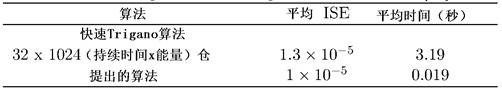
4.2 true data
The estimator is applied to the real data to evaluate its usefulness in practical applications. The threshold value found in (8) Is selected as additive noise
 Approximately half of the standard deviation of (c). This ensures that a reasonably high probability of creating an interval is created, which in turn ensures that the error of the interval energy estimate is low. The value of the interval length L is chosen to be approximately four times the "length" of a typical pulse, i.e., the interval length
 Four times that of the prior art. Obtaining an energy histogram from a manganese sample, where the photon flux rate is nominally 10 per second5An event. There was a slight negative skew in the shape of the observed histogram main peak, indicating that a complex noise source affected the system. This is hardly visible in fig. 8. The noise is modeled as a bimodal gaussian mixture rather than a single gaussian peak. Fitting bimodal Gaussian parameters using a simple least squares optimization routine
 The noise peak is located around bin index zero. Manually select
 A suitable value of. The true density is estimated using a logistic filter with a data-driven bandwidth. Fig. 8 shows a graph of observed and estimated probability mass vectors. The main peaks (bins 450-600) are enhanced and the build-up is not completely eliminated but attenuated. The first order stacking peak has decreased. The peak packing ratio (ratio of major peak height to first packing peak height) increased from about 6 to about 120. These improvements are in conjunction with other state-of-the-art systems (e.g. [11]]) And (4) the equivalent. There are several possible reasons for the estimator to fail to fully account for the pile-up. The accuracy of the estimate depends on correctly modeling the gaussian noise peaks.
Bimodal gaussian mixtures model the noise peak such that the maximum error is less than 1% of the noise density peak. Given that the residual piled-up peaks in the estimated spectrum are below 1% of the main peak, the sensitivity of the estimator to errors in the noise modeling may contribute to this in some parts. A second cause of unresolved pile-up may be due to uncertainty in the observed spectral estimate. Several residual piled-up peaks are relatively close to the bottom of the observed histogram. The residual peak may be just an artifact caused by the noise of the estimate. Finally, the mathematical model may be an overly simple approximation of the observed spectrum. The detection process includes many second-order effects not included in the model (e.g., ballistic deficit, supply charge depletion, correlated noise, non-linearity, etc.). These minor effects may limit the accuracy of the pile-up correction estimate.
5 overview of the first embodiment
We have adopted Gugushvili [18]]The proposed estimator for decomposition under gaussian noise is adapted for correcting pulse pile-up in the X-ray spectrum. We propose an easily implemented data-driven bandwidth selection mechanism and extensive sample counting of interest across spectral applications (10)4~109Count) range provides a significant reduction in ISE/MISE. Data driven rectangular bandwidth selective interfaceNear optimal (for rectangular filters) and better than bandwidth selection based on asymptotic results or fixed bandwidth in the range of interest.
Although the initial results seem promising, further work is required to improve the performance of the actual implementation. This estimate still contains the "ringing" artifacts associated with gibbs phenomena. Additional filter shapes attempt to reduce this, and there are other shapes that are closer to the MSE optimum.
6 second embodiment
This section gives an overview of the energy spectrum estimator of the second embodiment. The second embodiment solves the problem of the first embodiment that requires approximately the entire cluster to be contained in each interval. In a second embodiment, the entire data sequence can be used if desired, and the overlap compensated by introducing 2 different interval lengths L and L1.
We need to include some additional terms not mentioned in the first embodiment. In particular . Energy spectrum estimator based on

Filter Allows us to solve several implementation problems that arise. The estimation process we use can be summarized in the following steps.
1. Partitioning a sample time sequence into fixed-length intervals 。
。
2. According to For each interval being calculated
 The value is obtained.
3. From Value generating histogram
 。
。
4. Use of Inverse FFT computation of
 。
。
5. Partitioning a time series of samples to have a length L1And following similar calculations to obtain 。
。
6. Computing And
And 。
。
7. use of And
And computing
 。
。

8. Computing ,
, A low-pass filtered version of (a).
9. Computing 。
。
10. Use of Computing
 。
。
11. Use of And
And computing
 . If it is not
 Is zero, and
 is non-zero, the estimation fails because the discriminating logarithm is undefined.
12. Use of Is calculated according to

6.1 details of the Algorithm
Partitioning detector output stream into lengthsLOf non-overlapping sets of intervals, i.e. . Let
. Let Is the sum of the detector output samples in the jth interval, i.e.,

suppose thatLThe jth interval may contain "full" pulses as well as pulses truncated by the end of the interval, greater than the pulse length. It can be shown that, by us using
 Energy of the "complete" pulse represented, we use
 Truncated pulse and noise of representation
 The superposition of the energies of (a) and (b).
Partitioning the detector output stream into a second set of non-overlapping intervals Wherein
 . Let
. Let Is given by

If L is1Is selected to be slightly less than the pulse length, then Terms will not contain "complete" pulses, but only truncated pulses
 And noise
 The superposition of the energies of (a) and (b). The number of truncated pulses in any interval has a poisson distribution. We have

We can put the interval The total energy in (a) is decomposed into energy contributions from the truncated pulses
 And from being completely contained in the space
 Energy contribution of the pulse in (1)
 That is to say that,

wherein the content of the first and second substances, indicating that the pulse is completely contained in the interval (length is
 ) In a region of (a), and
 indicating that the pulse is truncated (length of
 ) Noise in the region of (a). Therefore, the temperature of the molten metal is controlled,

by combining (103) and (105), we have

Rearrangement gives

We can use a similar estimation to us Or some other method to estimate
 E.g. via empirical characteristic functions or by pairs
 The normalized histogram of values performs an FFT.
Reduced interval length when performing a decomposition operation Poisson's ratio of
 For taking into accountOn which the composite poisson process takes place
 Is used to measure the sub-interval of (1).
6.2 visualization of internal quantities
To assist the reader in understanding, FIG. 9 plots the various quantities obtained during the estimation process. The upper blue curve (value at bin zero is about 0.3) plots And observing an estimated characteristic function of the spectrum. Brown curve for showing
 The true value of (a), which is in the region [6000, 10000%]Clearly visible as the lower curve with periodic nulls. Number of
 Shown as a transparent red color and appearing as "noise" with an average density of
 Peaks are reached around the bin.
 The expected value of (c) is shown by a black dashed line. This is obtained as follows: use (75), known
 Values and are assumed to be known
 To obtain
 Gaussian noise. Number of
 Shown by a transparent blue curve. This is hardly visibleBecause it is at the
 interval 0, 4000],[12000,16000]Neutralization of Closely coincident and at intervals [5000,11000]Neutralization of
 Closely overlapping. It is noted that,
 the color of (1) appears at intervals [5000, 11000 ]]The inner color changes from red to purple because the two transparent drawings overlap. Solid black line shows
 It is
It is A low-pass filtered version of (a). As described in the paragraph opening in this section on smoothing, the low pass filtering removes noise due to peak positions
 Any local oscillation in (c). Item(s)
 Is used as
 Is estimated. It can be seen that
 In the region of (a) of (b),
 provide for
 Reasonably good estimation. When these two quantities are close to each other, the quality of the estimate degrades until eventually dominated by noise. Filter with a filter element having a plurality of filter elements
 Shall comprise
 While excluding bad estimates. To find out to obtain
 In a well-estimated area, we solve the following problem: given a
 In a local area
 Mainly from what the probability of noise occurrence is.
7 count rate estimation
Previous estimator assumptions Are known. Without a priori knowledge, pairs can be obtained as follows
 Is estimated.
1. Using from the previous section Calculating

2. Use of And estimating the counting rate. This can be done in a number of ways.
3. One way is to fit a curve to be a function of the optimization routine or some other means . The fitted parameters can be used to obtain an estimate of the count rate.
4. Another approach involves estimating DC offset of (1). This can be done by combining the appropriate number of
 The points are averaged to complete. By passing in the preceding section
 Filtering the obtained points is generally suitable, although fewer points may also yield sufficient estimates.
5. Another approach involves using an optimization engine or some other means to fit a curve to . Fitting
 Is given by

Wherein
And wherein Is selected to allow the curve to fit with sufficient accuracy. Parameter(s)
 An estimate of the count rate is provided. Optimization engine does not need to pair
 Each point in (a) is given equal weight.
8 description of the figures
The following figures help to understand the process. Fig. 1 shows one possible scheme for partitioning the detector output. The graph depicts the response of the sampling detector to three incident photons. To make the figure clearer, the effect of the noise has been removed. The output response is partitioned into several regions of equal length (L). The number of pulses arriving in each region is unknown to the processing system. One pulse arrives in the first interval. In the second interval two pulses arrive. In the third interval no pulses arrive. The total photon energy arriving in each interval is calculated as the statistic of interest, being the sum of all sample values in each interval. The intervals are not temporally aligned with the pulse arrivals. Fig. 2 illustrates the output of the estimation process. The true probability density of the incident photon energy is plotted as a solid black line. The photon arrival rate is such that at any given interval The inner average is reached by three photons. Output signal of detector
 The standard deviation of additive noise is equal to one histogram bin width. One million intervals were collected. A histogram of the total energy in each interval is plotted. This is plotted with a blue line. The effects of the pile-up are clearly evident, particularly around the
 bins 75, 150 and 225. The red trace plots the estimate of the true incident spectrum after the system processes the data. Although some noise is present in the estimation, the effects of the pile-up have been removed. This estimate is expected to correctly recover the true incident spectrum on average. The result is obtained using an internal filter whose bandwidth is automatically determined from the data. Fig. 3 illustrates the same number as fig. 2 under the same operating conditions, however in this case the bandwidth of the internal filter is determined using asymptotic results from the literature. Although the estimated incident energy probability density has beenRecovered, but the variance was significantly larger compared to fig. 2. FIG. 8 illustrates the operation of the system on real data. The blue trace plots the probability density of the observed energy value, while the red trace plots the estimated true probability density of the incident photon energy. There are no black traces, since the true probability density is unknown. In this experiment, the X-ray fluorescence of a manganese sample was used as a photon source. Photon arrival rate of about 10 per second5One photon. The interval length is chosen such that the average time between photons corresponds to the length of two intervals. Enough data is collected and partitioned to form 5.9xl06The interval of (c). The standard deviation of additive noise corresponds to 4.7 histogram bins. The estimation process clearly reduces the piled-up peaks and enhances the true peaks. Fig. 9 illustrates various quantities obtained during the simulation of the system described in the second embodiment. It is described in section 5.1 "visualization of internal quantities". Fig. 9-12 relate to a second embodiment. Fig. 10 illustrates the probability densities of the observed and true input photon energies of this experiment, from which fig. 9-13 were derived. The black trace plots the true probability density. The red trace plots the expected observed density when an average of three photons arrive within a given interval length. The blue trace plots the actual observed density. Packing up to tens of orders of magnitude can be seen in the observed densities. Fig. 10 includes several plots generated from a typical spectroscopy system. The actual incident photon density ("ideal density") is plotted with a solid black line. The observation histograms obtained by partitioning the time series data are shown in dark blue. The spectral distortion caused by pulse pile-up is significant. Fig. 13 plots the various internal quantities using a logarithmic vertical axis. The dark blue curve inclined toward the center of the drawing is . The amount of green horizontally crossing the plot is
 . The upper cyan curve, which is inclined toward the center of the drawing, is
 . FIG. 11 is a drawingShow a curve
 A trajectory in the complex plane. Fig. 12 illustrates internal quantities similar to fig. 9, however there are some additional signals. The horizontal red trace, mainly noise, and the corresponding black dashed representation
 The magnitude of the characteristic function of the histogram noise. A transparent green plot forming a "noise peak" in the center of the plot is an estimate
 . This quantity is plotted in blue in fig. 9 and is hardly visible, since it is not shown in fig. 12
 Is shielded. The horizontal trace having an average value of-3 is
 Drawing. The cyan color track is
 The magnitude of the eigenfunction of additive gaussian noise, which starts at zero at the zero bin and slopes to a minimum around 8000 bins. FIG. 13 relates to a second broad aspect of calculating count rates. It illustrates in computing
 The internal amount used. The cyan color track is
 The magnitude of the eigenfunction of additive gaussian noise, which starts with a zero value at bin zero and slopes to a minimum around 8000 bins. The dark blue trace, which slopes to a minimum at the center of the plot, is
 It isIs an estimate of the characteristic function of the observed data. The yellow/green horizontal trace with an average of-3 is
 Is estimated.
Reference to the literature


Claims (19)
1. A method of determining an energy spectrum of a single radiation quantum received in a radiation detector, the method comprising the steps of:
(1) obtaining a time series of digital observations from a radiation detector, the time series comprising pulses corresponding to individual quantum detections;
(2) calculating power spectrum sensitivity statistics from the detector signals, the power spectrum sensitivity statistics defining a mapping from pulse amplitude density to power spectrum sensitivity statistics; and
(3) the energy spectrum is determined by applying the inverse of the mapping to the spectrum sensitive statistics to estimate the density of pulse amplitudes.
2. The method of claim 1, further comprising basing energy spectrum sensitive statistics on a sum of digital observations over a plurality of time intervals.
3. The method of claim 2, further comprising defining the mapping using an approximate composite poisson process.
4. The method of claim 3, further comprising enhancing the approximate composite Poisson process by modeling noise.
5. The method of claim 4, further comprising expressing the mapping as a relationship between a characteristic function of amplitude, energy spectrum sensitive statistics, and modeled noise.
6. The method of claim 5, further comprising computing a feature function of the spectrum sensitive statistics by applying an inverse Fourier transform to a histogram of a sum of digital observations.
7. The method of claim 5 or claim 6, further comprising calculating a characteristic function of the amplitude with a low pass filter.
8. The method of any of claims 2 to 7, further comprising selecting each of the plurality of time intervals to contain zero or more approximately complete pulse clusters, and defining the plurality of time intervals as non-overlapping and of constant length L.
9. The method of claim 8, further comprising requiring a maximum value of the detector signal at the beginning and end of each time interval.
10. The method of claim 8 or 9, further comprising defining an approximate composite poisson process as a sum of pulse amplitudes in each time interval.
11. The method of any of claims 8 to 10, further comprising formulating a map as defined by equations (40) and (41).
12. The method of claim 11, further comprising enhancing the mapping by a windowing function.
13. The method of any of claims 2 to 7, further comprising selecting the plurality of intervals to comprise: a first set of non-overlapping time intervals of constant length L without regard to the entirety of the pulse cluster; and a second set of non-overlapping time intervals of constant length L1 less than L without regard to the entirety of the pulse cluster; where L is at least as long as the duration of the pulse.
14. The method of claim 13, further comprising selecting L1 to be less than the duration of the pulse.
15. The method of claim 13 or claim 14, further comprising approximating a composite poisson process as set forth in section 6.
16. The method of any of claims 13 to 15, further comprising a representation mapping as set forth in section 6.
17. The method of any one of claims 1 to 16, further comprising using a data-driven strategy selected to result in a near-optimal selection of a nuclear parameter that minimizes the integrated square of the error of the estimated probability density function of the energy of a single quantum of radiation.
18. A method of estimating a count rate of individual radiation quanta received in a radiation detector, the method comprising the steps of:
(1) obtaining a time series of digital observations from a radiation detector, the time series comprising pulses corresponding to individual quantum detections;
(2) calculating energy spectrum sensitivity statistics from the detector signals based on a sum of the digital observations over a plurality of time intervals, the energy spectrum sensitivity statistics defining a mapping from pulse amplitude density to energy spectrum sensitivity statistics using an approximate complex poisson process, the plurality of time intervals comprising: a first set of non-overlapping time intervals of constant length L, selected without regard to the entirety of the pulse cluster; and a second set of non-overlapping time intervals of constant length L1 less than L, also selected without regard to the entirety of the pulse cluster; wherein L is at least as long as the duration of the pulse interval;
(3) determining an estimate of a characteristic function of the approximated composite poisson process by equation (99);
(4) the count rate is estimated from an estimate of the characteristic function.
19. The method of claim 18, further comprising estimating a count rate by: an optimization routine or other means is used to fit the curve, estimate the DC offset of the estimated logarithm of the characteristic function, or fit the curve to the estimated logarithm of the characteristic function.
Applications Claiming Priority (3)
| Application Number | Priority Date | Filing Date | Title |
|---|---|---|---|
| AU2019900974 | 2019-03-22 | ||
| AU2019900974A AU2019900974A0 (en) | 2019-03-22 | Radiation detection with non-parametric decompounding of pulse pile-up | |
| PCT/AU2020/050275 WO2020191435A1 (en) | 2019-03-22 | 2020-03-23 | Radiation detection with non-parametric decompounding of pulse pile-up |
Publications (1)
| Publication Number | Publication Date |
|---|---|
| CN113826030A true CN113826030A (en) | 2021-12-21 |
Family
ID=72608371
Family Applications (1)
| Application Number | Title | Priority Date | Filing Date |
|---|---|---|---|
| CN202080037871.4A Pending CN113826030A (en) | 2019-03-22 | 2020-03-23 | Radiation detection with pulse pile-up nonparametric decomposition |
Country Status (8)
| Country | Link |
|---|---|
| US (1) | US20220137111A1 (en) |
| EP (1) | EP3942337A4 (en) |
| JP (1) | JP7291239B2 (en) |
| CN (1) | CN113826030A (en) |
| AU (1) | AU2020249184B2 (en) |
| CA (1) | CA3134143A1 (en) |
| IL (1) | IL286443A (en) |
| WO (1) | WO2020191435A1 (en) |
Family Cites Families (8)
| Publication number | Priority date | Publication date | Assignee | Title |
|---|---|---|---|---|
| NL7110516A (en) * | 1971-07-30 | 1973-02-01 | ||
| US6590957B1 (en) * | 2002-03-13 | 2003-07-08 | William K. Warburton | Method and apparatus for producing spectra corrected for deadtime losses in spectroscopy systems operating under variable input rate conditions |
| FR2870603B1 (en) | 2004-05-19 | 2006-07-28 | Commissariat Energie Atomique | MEASUREMENT AND PROCESSING OF A SIGNAL COMPRISING ELEMENTARY PULSE STACKS |
| CA2621736C (en) | 2004-09-16 | 2018-07-31 | Southern Innovation International Pty Ltd | Method and apparatus for resolving individual signals in detector output data |
| US10304217B2 (en) * | 2012-07-30 | 2019-05-28 | Toshiba Medical Systems Corporation | Method and system for generating image using filtered backprojection with noise weighting and or prior in |
| DE102013213362A1 (en) | 2013-07-08 | 2015-01-08 | Fraunhofer-Gesellschaft zur Förderung der angewandten Forschung e.V. | Method for identifying and quantifying emitting particles in systems |
| US10621756B2 (en) * | 2017-01-13 | 2020-04-14 | Canon Medical Systems Corporation | Apparatus and method for correcting bias in low-count computed tomography projection data |
| JP6912304B2 (en) * | 2017-07-20 | 2021-08-04 | 株式会社日立製作所 | Wave frequency distribution acquisition device, wave frequency distribution acquisition method, wave frequency distribution acquisition program and radiation imaging device |
-
2020
- 2020-03-23 WO PCT/AU2020/050275 patent/WO2020191435A1/en active Application Filing
- 2020-03-23 CA CA3134143A patent/CA3134143A1/en active Pending
- 2020-03-23 EP EP20777486.0A patent/EP3942337A4/en active Pending
- 2020-03-23 JP JP2021556719A patent/JP7291239B2/en active Active
- 2020-03-23 US US17/593,312 patent/US20220137111A1/en active Pending
- 2020-03-23 CN CN202080037871.4A patent/CN113826030A/en active Pending
- 2020-03-23 AU AU2020249184A patent/AU2020249184B2/en active Active
-
2021
- 2021-09-15 IL IL286443A patent/IL286443A/en unknown
Also Published As
| Publication number | Publication date |
|---|---|
| JP2022528512A (en) | 2022-06-14 |
| JP7291239B2 (en) | 2023-06-14 |
| AU2020249184A1 (en) | 2021-06-24 |
| EP3942337A1 (en) | 2022-01-26 |
| US20220137111A1 (en) | 2022-05-05 |
| EP3942337A4 (en) | 2022-12-21 |
| AU2020249184B2 (en) | 2021-09-16 |
| CA3134143A1 (en) | 2020-10-01 |
| WO2020191435A1 (en) | 2020-10-01 |
| IL286443A (en) | 2021-10-31 |
Similar Documents
| Publication | Publication Date | Title |
|---|---|---|
| Van Hateren et al. | On the genetically meaningful decomposition of grain-size distributions: A comparison of different end-member modelling algorithms | |
| JP5111105B2 (en) | Measurement method and analysis apparatus including signal processing including a chain of main impulses | |
| RU2681377C1 (en) | Method and apparatus for resolving signals in data | |
| US20060157655A1 (en) | System and method for detecting hazardous materials | |
| Ansari et al. | Correction of highly noisy strong motion records using a modified wavelet de-noising method | |
| JP2008513740A (en) | Apparatus and method for separating individual signals in detector output data | |
| CN110542406B (en) | Improved gyroscope signal denoising method based on EMD-MPF | |
| Sepulcre et al. | Sparse Regression Algorithm for Activity Estimation in $\gamma $ Spectrometry | |
| EP3637150A1 (en) | Gamma-ray spectrum classification | |
| US10156647B2 (en) | Method of spectral data detection and manipulation | |
| EP2433155B1 (en) | Radiation detection | |
| CN113826030A (en) | Radiation detection with pulse pile-up nonparametric decomposition | |
| Lavielle et al. | A simulated annealing version of the EM algorithm for non-Gaussian deconvolution | |
| Mclean et al. | Non-parametric decompounding of pulse pile-up under gaussian noise with finite data sets | |
| RU2802542C2 (en) | Radiation detection using nonparametric expansion of superimposed pulses | |
| US8676744B2 (en) | Physics-based, Bayesian sequential detection method and system for radioactive contraband | |
| Trigano et al. | Statistical pileup correction method for HPGe detectors | |
| Unser et al. | Maximum likelihood estimation of liner signal parameters for poisson processes | |
| Guo et al. | Structure-oriented filtering for seismic images using nonlocal median filter | |
| McLean et al. | Limitations of decision based pile-up correction algorithms | |
| Lopatin et al. | Pileup attenuation for spectroscopic signals using a sparse reconstruction | |
| Fu et al. | The application of wavelet denoising in material discrimination system | |
| CN116541668B (en) | Swimming stroke number determining method, device, equipment and storage medium | |
| EP0990216A1 (en) | Method of analyzing capabilities of multiple-suppression computer seismic data processing software | |
| Neuer et al. | A Cognitive Filter to Automatically Determine Scintillation Detector Materials and to Control Their Spectroscopic Resolution During Temperature Changes |
Legal Events
| Date | Code | Title | Description |
|---|---|---|---|
| PB01 | Publication | ||
| PB01 | Publication | ||
| SE01 | Entry into force of request for substantive examination | ||
| SE01 | Entry into force of request for substantive examination |