Background
At present, the research work of machine learning mainly focuses on non-incremental batch learning, and the learning method is to pack collected data into a data set according to batches and train a base learner in a centralized manner. With the mass increase of data, the storage cost of the data is continuously increased by reading and processing the data in a traditional data set form, and meanwhile, the data has hysteresis due to a centralized training mode, the working condition at the current time cannot be reflected in time, and the change condition of the data along with the time cannot be reasonably fed back. The online learning algorithm updates the learner based on a single sample or a batch of samples, and further expects to obtain an assumption based on all the samples at present, which is more suitable for practical problems.
In fact, however, in the online learning process, the data does not always satisfy the same distribution, and therefore, the statistical characteristics of the data also change in some way with time, and the prediction experience obtained based on the historical data may not be suitable for the current decision, which may result in the prediction accuracy of the learner being reduced. This phenomenon, in which the predicted result cannot be matched with the real data over time, is called concept drift, and is essentially that the statistical properties of the data change over time.
For the detection of concept drift, there have been studies involving three learning strategies, namely, sample selection, sample weighting, and multi-concept ensemble learning. The most common processing method is sample selection, and a window method is adopted, namely, some newly arrived samples are analyzed in a window to see whether a difference exists between the new sample and the old data.
On the basis of error detection of SVR, a method for detecting whether concept drift exists between samples through distribution similarity of Euclidean distances between the samples by using three hypothesis detection types is provided. The method is implemented by different modules by setting a fixed window and a variable window. The two windows have different detection tasks, parameters and window sizes do not need to be adjusted, and each window calculates a new sample in sequence, so that the calculation cost can be saved, and the detection capability can be obtained more quickly.
For the real process, the characteristics of the real process can change along with the change of the environment and the time, and the phenomenon also indicates that the concept contained in the data changes. If the customer's interest in purchasing a good may change over time, the amount of visits to the web site may also vary depending on the time period, and the concentration of MSWI process outlet NOx may have variability due to seasonal variations and adjustments in process conditions. This change is called a conceptual drift or data drift.
Precisely, for a given series of tagged itemsUntil time k, the historical data X ═ X1,x2,...,xk]The general learning objective is to build a base learner and train from these historical data to predict the output as accurately as possible, i.e., by x, when the data arrives at the next time k +1k+1Prediction of yk+1。
Sample x for the next time instant
k+1It can be considered to come from the overall hypothesis S
k+1The historical data satisfies the global assumption S
k. When new and old data obey the same distribution, S
k=S
k+1When the representative data is stable, S is
k≠S
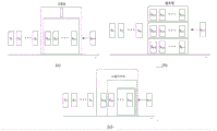
k+1When the data is not consistent with the same distribution, namely the data is unstable, and concept drift occurs. This process is illustrated in FIG. 1, wherein
Is a predicted value.
Hypothesis testing is a method for deducing the quantitative characteristics of a population from sample data, and is used for judging whether the difference between samples and populations is caused by sampling errors or intrinsic differences, wherein the sampling errors and the intrinsic differences can be respectively understood as noise and distribution change in the drift phenomenon. The purpose of the hypothesis test is to eliminate the effect of sampling errors and determine whether the difference between samples is statistically valid. The principle is to make some assumption about the characteristics of the population and to infer from sampling studies that the assumption should be rejected or accepted. Common test hypothesis types include F-test, t-test, rank-sum test.
The F test is also called joint hypothesis test and variance homogeneity test, and judges the sample correlation according to the variance correlation degree between samples to provide variance basis for other test methods. The variances of sample M and sample N are respectively
And
at a confidence level
F, statistical result F
F-testComprises the following steps:
the t test is used for testing the difference of the average values of the samples, and the probability of the occurrence of the difference is deduced through a t distribution theory, so that the significance of the difference of the two average values is judged, and the correlation between the samples is further judged. When samples have the same variance
At a confidence level
Then, the test result f
t-testComprises the following steps:
wherein μ
0Is the difference between the two sets of sample population averages, S
M and S
NThe number of elements of the two groups of samples,
and
is the sample average.
One of the common methods of rank-sum test is the mann-whitney U test, which is a non-parametric test method, and infers the overall distribution morphology using the sample when the overall variance is unknown. At the confidence level
Then, the test result f
U-testComprises the following steps:
wherein ZMIs the rank sum of sample M.
Whether the difference among the three test results is significant or not is analyzed, and the confidence levels of the three tests are preset
The confidence level represents an acceptable error range of hypothesis testing, when the confidence level is too small, the distribution testing is sensitive to concept change, and when slight differences exist among samples, the samples are difficult to pass the testing, so that drift misjudgment is caused, and the updating load of the learner is increased; when the confidence level is too high, the concept change is shown to be tolerant by the distribution test, so that the drift is missed to judge, and the prediction effect is reduced. Thus in a statistical test, a confidence level is typically chosen
Disclosure of Invention
Fig. 3 is an algorithm structure herein. Wherein X ═ X1,x2,...,xk]Representing historical data used to train the learner. Learner slave sample xk+1Initially, a sample-by-sample prediction is performed over time, as sample xk+wWhen detected as outliers, the current w samples are compared with the historical data in a distribution manner. w is at the same time the size of the variable window, depending on the sample size from the first starting sample to the anomalous sample.
Conceptual drift is easily confused with noisy data, as both bias the data analysis, but the noise is still from the same assumed population as the historical data. Therefore, proper discrimination of noise is a primary task to deal with the concept drift problem.
The first window is used for outlier detection in order to find prediction anomalies in time to start the distributed detection window. The window receives the latest one sample at a time, so the window size is set to one sample size, and SVR is used for detection in the window.
The SVR is regression analysis established on the support vector, has the advantages of strong generalization ability and high learning speed, and has the loss function LlossComprises the following steps:
wherein ,
and y
iThe predicted value and the true value on the training set are respectively, k is the number of training samples, and epsilon is an insensitive function and represents the range of acceptable errors. By introducing lagrange multiplier alpha
iAnd
optimizing the regression problem to obtain an SVR function:
wherein k*For the number of support vectors, b is the offset:
establishing an SVR estimation model by using historical samples in a window, performing regression estimation on the latest data, judging whether the sample is an outlier according to whether the error e is greater than the threshold value xi, and if so, determining whether the sample is an outlier
And sending an alarm to the distribution detection window.
Calculating an error threshold xi:
ξ=(eM-eL)×0.4
wherein ,eMMaximum prediction error so far, eLThe prediction error of the last sample.
wherein ,
when the threshold value xi is too small, the outlier detection window can alarm frequently, the distribution detection window is in a detection state for a long time, the calculation time is increased, and the detection efficiency is reduced; when the threshold ξ is too large, the alarm frequency of the outlier detection window is reduced, the distribution detection window possibly misses a sample which begins to drift, and the detection efficiency is reduced. Therefore, a reasonable threshold value is selected according to the fluctuation condition of the data in a stable state, so that the prediction precision can be increased, and the distribution detection efficiency can be improved.
And when the outlier detection window detects abnormality and sends an alarm signal, the distribution detection window matches the samples in the window with the historical samples to judge whether the alarm comes from concept drift. In the window, the Euclidean distance between the self samples in the historical samples and the Euclidean distance between the samples in the window and the historical samples are firstly calculated. In Euclidean space, sample xi=[xi1,…,xiP]And sample xj=[xj1,…,xjP]The euclidean distance (j ═ 1,2, …, k) is:
where P represents the number of features per sample,
and
respectively indicate the distance D between original samples
OldAnd new and old sample distance D
NewThe variance of (a) is determined,
DOld=[d11,d12,…,d1k,…,dk1,dk2,…,dkk](9)
DNew=[d1k+1,d1k+2…d1k+w…dkk+1dkk+2dkk+w](10)
the two sets of distances were then analyzed for homogeneity of variance using the F-test:
f-check return value
Is composed of
When in use
Both distance sample variances
Then, the average of the two sets of distances was further analyzed using a t-test:
wherein μ
ONIs the difference between the mean values of two sets of distance sample populations, S
Old and S
NewThe number of elements in the two sets of distance samples, respectively. t check return value
Comprises the following steps:
when in use
When the two sets of distances have the same distribution, otherwise the distributions are considered different.
For two groups of distances with different variances, judging by adopting a ManWhitney U test, and testing the return value
Comprises the following steps:
when in use
When the two sets of distances have the same distribution, otherwise the distributions are considered different. The conditions under which the distribution changes are:
when concept drift occurs, the data distribution changes, and such changes are reflected in the change of the sample distance between the old and new data. The conceptual variation of the data can be indirectly reflected by the significant difference of the two groups of distances in the statistical property. If no distribution difference is detected in the second window, the alarm signal is considered to be caused by noise, thereby avoiding erroneous updating of the learner.
The verification process of the present method is depicted in fig. 4. And after a new sample arrives, testing the sample by using the trained SVR, considering that the data is not changed when the testing error is smaller than a threshold xi, and considering that the data is abnormal when the testing error is larger than the threshold xi. Then, Euclidean distances between the samples in the variable window and the historical samples are calculated, and whether the two groups of distance data have similarity in variance is observed through an F test. And when the variance is not significantly different, performing t test on the two groups of distance data, and judging the correlation and distribution condition between the two groups of samples according to the similarity of the average values of the two groups of distances. When there was a significant difference in variance, the drift condition between the two sets of samples was analyzed by the rank sum test.
Detailed Description
In order to verify the performance of the method, a cement strength benchmark dataset is selected for testing, and the data comes from a Prof.I-Cheng Yeh learning team and can be obtained by accessing UCI (https:// architectural.ics.uci.edu /). The data set contains 1030 samples, the input variables are main factors directly or indirectly influencing the compressive strength of the Cement, and are respectively Cement (center), Blast Furnace Slag (Blast Furnace Slag), Fly Ash (Fly Ash), Water (Water), a high-efficiency Water reducing agent (superplastic), Coarse Aggregate (Coarse Aggregate), Fine Aggregate (Fine Aggregate) and Age (Age), and the output is Concrete compressive strength (Concrete compressive strength).
Firstly, dividing a data set into two sub data sets, wherein the two sub data sets respectively comprise front 500 groups of data and rear 500 groups of data in an original data set, and then dividing the two sub data sets into five parts at equal intervals, wherein each part comprises 100 groups of data. The method uses the 1 st data in the first sub data set as a training set for modeling, and uses the 3 rd data, the 4 th data in the first sub data set and the 1 st data in the second sub data set as a test set 1, a test set 2 and a test set 3 respectively for testing. In the experiment, only the data is standardized, the feature selection is not carried out, and the data is fitted sample by sample during the test, so that the real-time processing environment is simulated.
Fig. 5 shows the fitting effect of the trained SVR to the training set, in which the kernel function is selected as rbf (radial Basis function), the penalty parameter is 1, the kernel width σ is 1, and the insensitivity μ is 0.001. The error threshold ξ is set at 25 (the threshold magnitude is chosen artificially according to the fitting error in fig. 6), i.e. the window issues an alarm when the fitting error exceeds 25.
Figure 6 shows the effect of the fit versus error curves on test set 1, test set 2 and test set 3. It can be seen that the first outlier appears on the 35 th sample, the 10 th sample and the 24 th sample of the three test sets respectively, and meanwhile, the fitting effect of the learner on the test sets 1 and 3 is stable, and the fitting effect fluctuation on the test set 2 is large. Due to the nature of SVR, the learner readily identifies samples with higher prediction errors, indicating that the first window of this document performs sensitively and accurately in detecting outliers.
The second window is used to calculate the distance between the samples in the training set, the distance between the test set 1 and the samples in the training set, the distance between the test set 2 and the samples in the training set, and the distance between the test set 3 and the samples in the training set. Performing F test, t test or Man-Whitney U test on the above 4 distance sets, and sequentially setting significance levels of the three tests
For the three test types, h-0 represents that the original hypothesis is accepted, namely that the same variance or average exists between two groups of distance data, and the correlation is strong; h-1 represents rejection of the original hypothesis, i.e., there is no identical variance or mean between the two sets of distance data, and there is no strong correlation. The value of h is determined by each check statistic and its corresponding table of threshold values. Tables 1-3 show the results of the three significance levels for the different test sets.
TABLE 1 hypothesis test results (α ═ 0.01)
TABLE 2 hypothesis test results (α ═ 0.03)
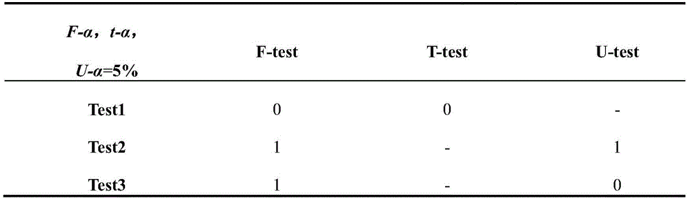
TABLE 3 hypothesis test results (α ═ 0.05)
According to the test result, the distance set corresponding to the test set 1 and the distance of the training sample have similar variance, and the t test is passed. The distance sets corresponding to test set 2 and test set 3 have different variances from the training samples' own distances, but test set 2 failed the U-test. The distribution diagram corresponding to each distance set is given in fig. 7.
Table 4 shows the distribution of the four sets of distances in different intervals. Therefore, the sample distance in the training set is concentrated in the interval of 0-0.5, and the sample distance between the test set 2 and the training set is smaller in the interval. This reveals that there is a conceptual drift between the data, verifying the validity of the distributed detection window.
TABLE 4 sample distribution over different distance intervals on the reference dataset
This document compares with the entropy-based conceptual drift detection method on a reference data set. In the two data sets, the ratios of 4 groups of distances falling within the range of 0-0.5, 0.5-1, 1-1.5, 1.5-2, 2-2.5 were calculated respectively, entropy values were calculated, and statistical test analysis was performed on the data within each range using the method herein, and the results are recorded in table 5.
TABLE 5 method comparison on reference data set
In the entropy-based method, when the data distribution is equal, the entropy value is 1, and when the data distribution is different, the entropy value is 0. In Table 5, the mean entropy of test set 2 is closer to 1, and the distribution is considered unchanged, while the distance distribution map and statistical test results obtained by the method herein show that test set 2 fails the rank-sum test in the range of 0-1, and the distribution is considered changed, which is also in accordance with the results of the learner's fitting to test set 2. Entropy-based methods therefore perform poorly on the testing of continuous type variables compared to statistical testing algorithms.
The industrial data here is from a MSWI power plant within the country. In the MSWI incineration stage, a large amount of flue gas including nitrogen oxides is generated, and in order to prevent the flue gas from forming secondary pollution, the concentration of the nitrogen oxides at the outlet can be predicted, and corresponding prevention and control measures can be taken in time according to the prediction result. However, the method is influenced by factors such as the content change of solid waste water in different seasons, the environmental change in the incinerator and the like, and the prediction model parameters of the discharge concentration of the nitrogen oxides under different working conditions may be different, so that the phenomenon accords with the concept drift problem to be solved.
The method takes the production end and the elimination end of the nitrogen oxide into consideration, selects 19 variables with the strongest correlation with the factors such as the hearth temperature, the primary air quantity, the secondary air quantity, the hearth residual oxygen quantity, the urea spraying quantity and the like, selects 1000 samples as a training set according to the time sequence, and divides 1500 samples into three test sets at equal intervals.
In the course of training the learner, a penalty parameter of 20, a kernel function width σ of 20, an insensitivity μ of 0.001, and significance levels of the three hypothesis tests are set as
The verification effect is as shown in fig. 8 and 9.
Fig. 9 shows the prediction and error curves on the industrial data set, and it can be seen that when the working conditions of the test set are the same as those of the training set, the learner predicts accurately, and when the working conditions are changed and the prediction concept changes, the prediction result has a large error. Hypothesis testing was further performed on the test set versus the training set at a significance level α of 0.05:
table 6 hypothesis test results (α ═ 0.05)
As shown in table 6, since the operating conditions in the three test sets are changed significantly, the distance distribution is different from the distance distribution in the training set in variance, and fails the F test, and fails the U test also indicates that there is a change in the distribution in the data, so there is a conceptual drift.
In fig. 10 and table 7, it can be seen that the distance distribution difference between the three test sets and the training set is represented by that in the distance range of 0-0.5, the sample proportion of the training set is higher, and the distance image of the three test sets is shorter in the interval, and more sample distances fall between 0.5-1. This also verifies the concept drift phenomenon in industrial data sets.
TABLE 7 sample distribution over different distance intervals on an industrial data set
This document compares equally with entropy-based detection methods on industrial datasets. In the two data sets, the ratios of 4 groups of distances falling within the range of 0-0.5, 0.5-1, 1-1.5, 1.5-2, 2-2.5 were calculated, entropy values were calculated, statistical test analysis was performed on the data within each range using the method herein, and the results are recorded in table 8.
TABLE 8 comparison of methods on Industrial data sets
For test set 2 in table 8, although the results of the two test methods are the same, the method herein can additionally reflect the variance change in the test set, and the variance represents the variation degree of the data, which provides an important basis for the subsequent update of the learner model. Therefore, compared with the entropy-based detection method, the method can give detailed statistical information on each interval, and the change amplitude and the change form of the whole data can be observed.
The influence of different parameters on the test results is mainly analyzed here. For threshold ξ: as can be seen from fig. 6, the size of the outlier detection window determines the alarm frequency, which affects the memory usage and computation power of the learner, and thus determines the prediction accuracy, which in turn affects the distribution verification efficiency.
For confidence level
As can be seen from tables 1 to 3, similar to the effect of the threshold ξ, the change in size thereof causes the sensitivity of the distribution inspection window to data changes to be different, affecting the timeliness of distribution detection.
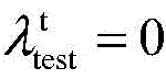
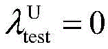
Return values for three tests
As can be seen from the above experimental results, when the prediction error is greatly increased, the variance of the distances between the data becomes unequal, that is
When the prediction accuracy rate continuously and greatly changes, the average value and rank and grade of the distance between the data are unequalI.e. by
And
as in Table 5 and FIG. 6, the prediction effect on test set 2 is greatly reduced, and F-test returns
While the prediction accuracy fluctuates frequently, its U checks the return value
Different distributions of data in test set 2 versus training set are revealed. Test set 3 with large prediction error, F-test return value
But the prediction accuracy is stable, and the return value is tested by U
In table 8 and fig. 9, the prediction error and the prediction accuracy on the three test sets each show large fluctuations, which all have
And
so F checks the return value
With the ability to track outliers, feedback can be made as the distribution may change. And the return values of t-test and U-test
And
having the ability to track distribution, the basis can be verified at FWhether the distribution changes is determined on the basis.
A double-window online concept drift detection method based on SVR detection and Euclidean distance statistical test is provided, and tests are carried out on a cement strength reference data set and an MSWI industrial data set. The main contributions herein are: (1) the method provides concept drift detection based on double windows, firstly, abnormal detection is carried out based on a first window, and then, real-time data distribution detection is carried out based on a second window by adopting 3 hypothesis testing modes; (2) it is proposed herein to reflect changes in data distribution indirectly through changes in distance between samples. The drift detection method will be integrated into an online learner in future work to solve practical problems related to time series.